1/30

String Stability Analysis of Adaptive Cruise Controlled Vehicles

Chi-Ying LIANG and Huei PENG

Key Words: Adaptive Cruise Control, String Stability, String Stability Margin,

Optimal ACC Design, Traffic Simulator

Department of Mechanical Engineering and Applied Mechanics,

University of Michigan

2272 G.G. Brown, Ann Arbor, MI 48109-2125, USA,

E-mail: hpeng@umich.edu

TEL: (734) 936-0352, FAX: (734) 647-3170

2/30

ABSTRACT

A framework for string-stability analysis is formulated in this paper. First,

uniform string will be analyzed. We will then present analysis results on strings of

mixed vehicles. A String-Stability Margin (SSM) index is defined in this paper to

give a quantitative measurement of any ACC design. Simulation results using

MATLAB and a microscopic traffic simulator will also be given to demonstrate the

effectiveness of ACC systems on traffic smoothness.

3/30

1. INTRODUCTION

Adaptive Cruise Control (ACC) system has been proposed as an enhancement

over existing cruise controllers on ground vehicles. ACC systems control the vehicle

speed to follow a driver’s set speed closely when no lead vehicle is insight. When a

slower leading vehicle is present, the ACC controlled vehicle will follow the lead

vehicle at a safe distance. ACC research first began in the 1960’s [1], and has

received ever-growing attention in the last decade. Their commercial implementation

is not possible until recently with significant progresses in sensors, actuators, and

other enabling technologies.

Over the last 10 years, many different approaches have been proposed for the

design of ACC algorithms. In the earlier works, the focus has been on the

performance of the host vehicle. The performance was usually evaluated based on 2-

car platoons. The effect of ACC on a string of vehicles has not received much

attention. Recently, a 2-step synthesis method was proposed which can be used to

design ACC algorithm with guaranteed stability [2]. At the upper level, desired

vehicle acceleration is computed based on vehicle range and range rate measurement.

At the lower (servo) level, an adaptive control algorithm is designed to ensure the

vehicle follows the acceleration command accurately. It is shown that it is possible to

include servo-level dynamics in the overall design and string stability can be

guaranteed if certain inequality constraints are satisfied.

The so-called “string stability” problem has been studied as early as 1977 [4].

The string-stability ensures that range errors decrease as they propagate along he

vehicle stream. It is widely known that when the transfer function from the range

error of a vehicle to that of its following vehicle has a magnitude less than 1, string

4/30

stability is guaranteed [5]. To achieve string stability with constant inter-vehicle

spacing, vehicle-to-vehicle communication was shown to be necessary [6]. Yanakiev

and Kanellakopoulos [7] used a simple spring-mass-damper system to demonstrate

the idea of string stability and show the string-stability criterion for constant time-

headway and variable time-headway policies. Swaroop and Hedrick [8] proved,

among many other interesting things that if the coupling between two vehicles is

weak enough, the controlled system is string stable.

Despite the strides made in the research field, many of the prototype ACC

vehicles were still designed without considering string stability. This is mainly due to

the fact that human drivers and passengers are used to the level of smoothness

produced by human drivers. The early implementation of ACC hardware is usually

marked by slow response of actuation and rough distance and speed measurement. In

order to produce smooth acceleration/deceleration response, the ACC controllers are

usually heavily filtered. Slower response from individual vehicles then results in

unstable string response.

In this paper, we plan to demonstrate a detailed stability analysis of a string of

vehicles. First, uniform string will be analyzed. Necessary and sufficient conditions

for string stability will be presented. We will then present analysis results on strings

of mixed vehicles. It will be shown that if we mix ACC vehicles that are designed to

be string stable by themselves, the mixed ACC strings will also be string stable. The

stability degradation will be shown in the context of the “string stability margin”

(SSM) which is an index defined to measure the string stability of a vehicle.

A simulation tool (UMACC) is developed in the University of Michigan to

assist the analysis of ACC system. This simulator is divided into four parts: driver

model, vehicle/sensor model, ACC model, and the interaction model (see Fig. 1). The

5/30

driver model consists of a lane change model (for all vehicles) and a car-following

model (only for manually controlled vehicles). The parameters of the driver model

are obtained from the FOCAS field test data [9]. Details of this model can be found

in [3].

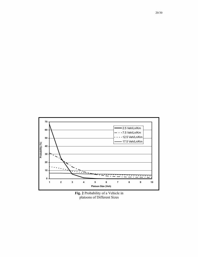
A simulation study using ACC Simulator has shown that the vehicle string

size increases dramatically with the traffic density (See Fig. 2,3). Because manual

vehicles are usually not string stable, the large platoon size in high traffic density will

magnify the so-called “slinky effect” and caused traffic jammed. A string stable ACC

design is able to reduce this slinky effect and thus improve highway traffic. In this

paper, the performance of ACC vehicles will be evaluated by mixing ACC vehicles

and manually controlled vehicles using the ACC Simulator. Simulation results using

the UMACC Simulator will be presented to highlight the effect of ACC vehicles on

the traffic volume and smoothness.

The remainder of this paper is organized as follows: the formulation of

vehicle-string analysis is presented in Section 2. In Section 3, both uniformed and

mixed vehicle strings will be analyzed. The definition of SSM and the SSM

calculation of an optimal ACC design will be given in Section 4. Representative

simulation results are given in Section 5.

2. PROBLEM FORMULATION

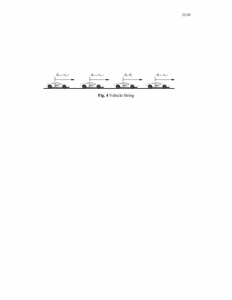
Considering a group of vehicles form a string in dense traffic where no

passing occur (Fig. 4) and assuming the operation of each vehicle looks only one

vehicle ahead, each vehicle in this string can be modeled as following:

Fig 4

Fig 1

Fig 2,3

6/30

1)(

1

−⋅=

=

iii

ii

vsGv

vs

x (1)

where vi is the velocity of the ith vehicle and Gi represents the car-following

algorithm of the ith vehicle (for both ACC vehicles or manual vehicles). For each

vehicle, the following errors are defined:

iiii Dxx −−= −1ε (Range Error)

iivi vv −= −1ε (Range Rate Error)

where Di denotes the desired range for the ith vehicle.

In this paper we have assumed constant time-headway policy is adopted for all

vehicles, that is, the desired ranges are proportional to vehicle speeds. Let iii vhD ⋅=

(hi is the constant time-headway for the ith vehicle), then the range errors can be

rewritten as:

iiiii vhxx ⋅−−= −1ε (2)

To investigate the string stability of such a system, a propagation transfer

function kiG , is defined as the transfer function from range error of ith vehicle to the

range error of the i+kth vehicle.

i

kikiG

εε +=, (3)

Substituting (1) and (2) into (3), we have

)1(

)1(11,

iii

kikikikiiiki GhsG

GhsGGGGG⋅⋅−−⋅⋅−−⋅⋅= +++

−++ (4)

7/30

Clearly, the propagation transfer function kiG , depends on the following

algorithms of all the vehicles between the ith vehicle and the i+kth vehicle. In the

derivation we have not specified Gi. Therefore, this general formulation can be used

to study the string stability of uniform vehicle strings as well as mixed vehicle strings

in the following section.

3. String Stability of Vehicle Strings

3.1. Uniform Vehicle Strings

Consider a uniform vehicle string, that is, all vehicles in the string are

identical, i.e. Gi = G and hi = h ∀ i. It is clear that the range error output must be

smaller than or equal to the range error input to avoid range errors propagate

indefinitely along the string. For this uniform vehicle string, a string-stability

definition is widely used [7] and is described as following:

Definition 1 (String Stability of A Uniform String):

A uniform vehicle string is string stable if

221 ii εε ≤+

Remark:

In a uniform vehicle string, the propagation transfer function 1,iG from the range error

(εi) of one vehicle to the range error (ει+1) of its follower can be written as:

GGGhsGGhsGGG i

iii

iiiii

i

i ==⋅⋅−−⋅⋅−−

⋅== ++++

)1()1( 111

1,1

εε

8/30

To achieve string stability, the inequality 1≤∞

G needs to be satisfied.

Therefore, the string stability of an uniformed vehicle string can be determined by the

car-following algorithm G.

3.2. Mixed Vehicle Strings

In the previous section, string stability is defined under the assumption of

uniform vehicle strings. On real highway, however, a vehicle strings consist of

different types of vehicles, including manual and automated, string stable and string

unstable vehicles. What is the string-stability property of such a mixed vehicle string?

More specifically, if we consider a mixed vehicle string consisted of string-unstable

manual vehicles and string-stable semi-automated vehicles, how can we define the

string stability of this mixed vehicle string? Clearly, the string-stability definition in

Definition 1 is not enough to answer these questions. In order to investigate this

problem, we first define string stability for mixed vehicle strings.

For a mixed vehicle string, the string stability from vehicle to vehicle has

become meaningless because no simple expression can represent all vehicles in this

mixed vehicle string. For example, if there are three vehicles in a string following a

lead vehicle (Fig. 5) and they are all string-stable under Definition 1 with a constant

time-headway h = 1 sec,

17.117.0)(

15.115.0)(

17.117.0)(

23

22

21

+++=

+++=

+++=

ssssG

ssssG

ssssG

with

Fig 5

9/30

1,1,1 321 ≤≤≤∞∞∞

GGG

the two propagation transfer functions are as follows

)1()1(

11

221

1

21,1 GhsG

GhsGGG

⋅⋅−−⋅⋅−−

⋅==εε

)1()1(

22

332

2

31,2 GhsG

GhsGGG

⋅⋅−−⋅⋅−−

⋅==εε

and we found that

1,1 1,21,1 <>∞∞

GG

It is obviously that no conclusion about the string stability of this mixed string

can be drawn in this numerical example. In the following, we will propose a string-

stability definition for mixed vehicle strings.

Consider a mixed vehicle string (S1) of k vehicles. If this string is repeated to

form an infinite string as in Fig. 6, then the propagation transfer function from the

first vehicle’s rang error (εnk+1) of one sub-string (Sn) to that (ε(n+1)k+1) of the

following sub-string (εn+1) is as follows:

)1()1(

111

1)1(1)1(1)1(21

1

1)1(,1

+++

+++++++++

+

+++

⋅⋅−−⋅⋅−−

⋅⋅=

=

nknknk

knknknknknknk

nk

knknk

GhsGGhsG

GGG

Gε

ε

(5)

∞= ..0n

Because kknknknk GGGGGG === +++ ,,, 2211 and 11 hhnk =+ , (5)

becomes

Fig 6

10/30

kknk GGGG 21,1 ⋅=+ ∞= ..0n (6)

It is clear that to avoid any range error being amplified unboundedly along this

imaginary infinite vehicle string, the magnitude of knkG ,1+ must be less than or equal

to 1. Therefore, the string-stability definition of a mixed vehicle string is stated as

follows:

Definition 2 (String Stability of Mixed Vehicle Strings):

A mixed vehicle string of k vehicles is string stable if 1,1 ≤∞+ knkG . That

is, 121 ≤⋅∞kGGG where Gi, i = 1 .. k, represents the car-following algorithms of

the ith vehicle.

Remark 1:

If a vehicle string is string stable and all vehicles in this string are identical, then each

vehicle must be string stable. It is obvious that Definition 1 is just a special case of

Definition 2.

Remark 2:

According to Definition 2, the string stability of a mixed vehicle string is not affected

by the position of individual vehicle in this string.

Theorem 1:

A mixed vehicle string is string stable if all vehicles in this string is string stable.

Proof:

∞∞∞∞∞⋅≤⋅= kkk GGGGGGG 2121,1

11/30

If all the vehicles are string stable, i.e. 1≤∞iG , i = 1..k, we have 1,1 ≤

∞kG .

From definition 2, this mixed vehicle string is string stable.

4. String Stability Margin (SSM)

String stability has become an important design issue in the vehicle

longitudinal control. Researches have been done on the proof and analysis of string

stability. However, no quantitative measurement of string stability has been provided.

As a result, there is no way we can determine if one ACC design is “marginally”

string stable? Or if one ACC design is more string stable than the other? In this

section, we will define a string-stability margin (SSM) and determine the string

stability of ACC designs in the context of SSM. The margin is basically measure of

how close an ACC design comes to the marginal string stability, i.e. 1=∞

G . The

operational definition of SSM is stated below

Definition 3 (String-Stability Margin):

Consider a mixed vehicle string consisting of n standard manual vehicles with their

car-following algorithm represented by GMV and an ACC controlled vehicle with its

car-following algorithm represented by GACC. Increase n from zero until nmax so that

the following inequality is not satisfied

1≤⋅⋅∞ACCMVMVMV GGGG

n

12/30

The nmax is the SSM for this ACC controlled vehicle.

Remark 1:

If nmax is equal to zero, then this ACC design is marginally string stable. The larger

nmax is, the more string-stable the ACC design is.

In order to measure SSM, the Pipes human driver model [12] is used as a

standard manual vehicle model.

[ ])()()( 1 ∆−−∆−⋅=⋅ − tvtvtvM iii λ

where M is vehicle mass, λ is the sensitivity of the control mechanism, and ∆ is the

time delay of human driver. From Chandler’s paper [10], the average value of λ/Μ is

equal to 0.368 and the average value of ∆ is equal to 1.55. The input-output behavior

of this human car-following model can be approximated by the following linear

transfer function

74.043.155.1

74.057.0368.0

368.0255.1

55.1

1 +++−≈

⋅+⋅==

−

−

− sss

ese

vv

Gs

s

i

iMV

In the following, we will examine the SSM for an optimal ACC algorithm

design [2], which considers not only the behavior of the controlled vehicle itself, but

also all its following vehicles.

Consider an infinite vehicle strings. Assume all the vehicles in this string are

identical and are under the same control strategy. Each vehicle can be represented by

the following dynamics equation:

kkkkk uBxAx += ∞−∞= ..k (7)

13/30

where

=

k

kk v

zx ,

=

0010

kA ,

=

10

kB , zk is the position of the kth vehicle and vk

is the velocity of the kth vehicle. When a constant time-headway policy is used, the

two major error terms are kdkk vhzz −−−1 (range error) and kk vv −−1 (range rate

error). Defining these two variables as outputs for each vehicle, we have

∑∞

−∞=−=

jjjkk xGy (8)

0,1,0,10

1,

1001

01 −≠∀=

−

−−=

=− kG

hGG k

d

If we use simple proportional control, the control law becomes

kkkkdkkk yKvvkvhzzku ⋅≡−⋅+−−⋅= −− )()( 1211 (9)

An optimal control framework can then be formulated to minimize the range

errors and range rate errors for all the vehicles in the string. A performance index can

thus be defined:

dtruvvqvhzzqJ kkkkdkkk

])()([21 22

122

0 11 +−+−−= −

∞

−

∞

−∞=∫ ∑ (10)

where q1, q2, and r are the design penalties on the range error, range-rate error, and

control effort respectively.

A bilateral z transformation technique [11] is applied to solve this optimization

problem. The dynamics equations are transformed to the following equations:

)()()()()( zuzBzxzAzx += (11)

)()()( zxzGzy = (12)

)()( zKyzu = (13)

14/30

The performance index in Eq. (10) can also be rewritten as

00

1 )),(exp(),()),(exp(21ˆ ∫

∞− ⋅⋅⋅= dttKzKztKztrJ T DMD (14)

where

)()()(),( zKzzKz GBAD += (15)

)()()()(),( 1 zKzKzzKz TT GRGQM −+= (16)

The objective of this optimization problem is to find an optimal gain K* that

minimizes the performance index J . K* can be solved by the following equation

using an iteration method.

1

0

11

0

11

)(),()()(),()(

)(),(),()()(),(),()(1

−−−

−−

+

⋅+−=

TTT

TTTTTT

zKzzzKzz

zKzKzzzKzKzzr

K

GLGGLG

GLPBGLPB (17)

where the matrices ),( KzP and ),( KzL are solved from the following algebraic

equations:

0),(),(),(),(),( 1 =++ − KzKzKzKzKz T MPDDP (18)

0),(),(),(),( 1 =++−n

T IKzKzKzKz LDDL (19)

More detailed derivation can be found in [2]. An advantage of this optimal

ACC design is that if there exists an optimal control gain K*, the gain is guaranteed to

make the controlled ACC vehicle string stable.

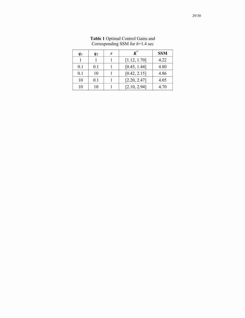
Table 1 shows the optimal control gains and their corresponding SSM values

under different penalties with the constant time-headway h = 1.4 sec.

Table 1

15/30

5. SIMULATION

In this section, the optimal ACC design described in Section 4 are

implemented for simulation studies. The desired constant time-headway in the

control design is selected to be 1.4 seconds, which is the average value taken from the

FOCUS field test data. The optimal control gain K* =[1.12,1.70] correspond to the

penalties q1 = 1, q2 = 1, and r = 1. Two different simulation tools are used to perform

a series of simulations to demonstrate the effectiveness of ACC systems on traffic

smoothness. First, we use MATLAB to simulate a platoon of 20 vehicles. These

simulations are based on the assumption that the lateral operations of all vehicles are

perfect. That is, disturbances due to lane changing /merging are not considered.

Second, the UMACC simulator is used to investigate the effectiveness of ACC

systems. In this simulation program, the vehicle longitudinal dynamics is simple, but

a complex lane change behavior is included. A two-lane closed-circuit highway is

constructed in which autonomous lane changes will occur. The fact that we are

simulating individual vehicles enables us to study safety and traffic-flow

characteristics more accurately.

5.1 MATLAB Study

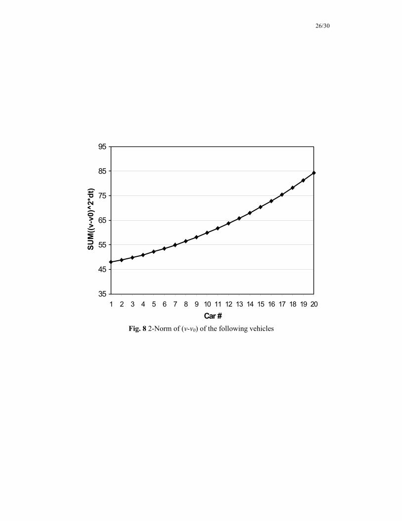
We first examine the transient behavior in dense manual traffic where a string

of 20 manual vehicles follow a lead vehicle in a single lane without passing. The

Pipes model is used to represent the manual vehicles. All vehicles start at a constant

velocity of 30 m/sec (67.5 mph) and then the lead vehicle accelerates to 32 m/sec (72

mph) and keeps at 32 m/s for 10 sec and decelerates back to 30 m/sec. The

acceleration is 1 m/sec2 and the jerk is limited to 20 m/s3. Figure 7 shows that the

16/30

Pipes (manual) vehicles exhibit slinky effect. Figure 8 shows that 20vv − is

amplified upstream.

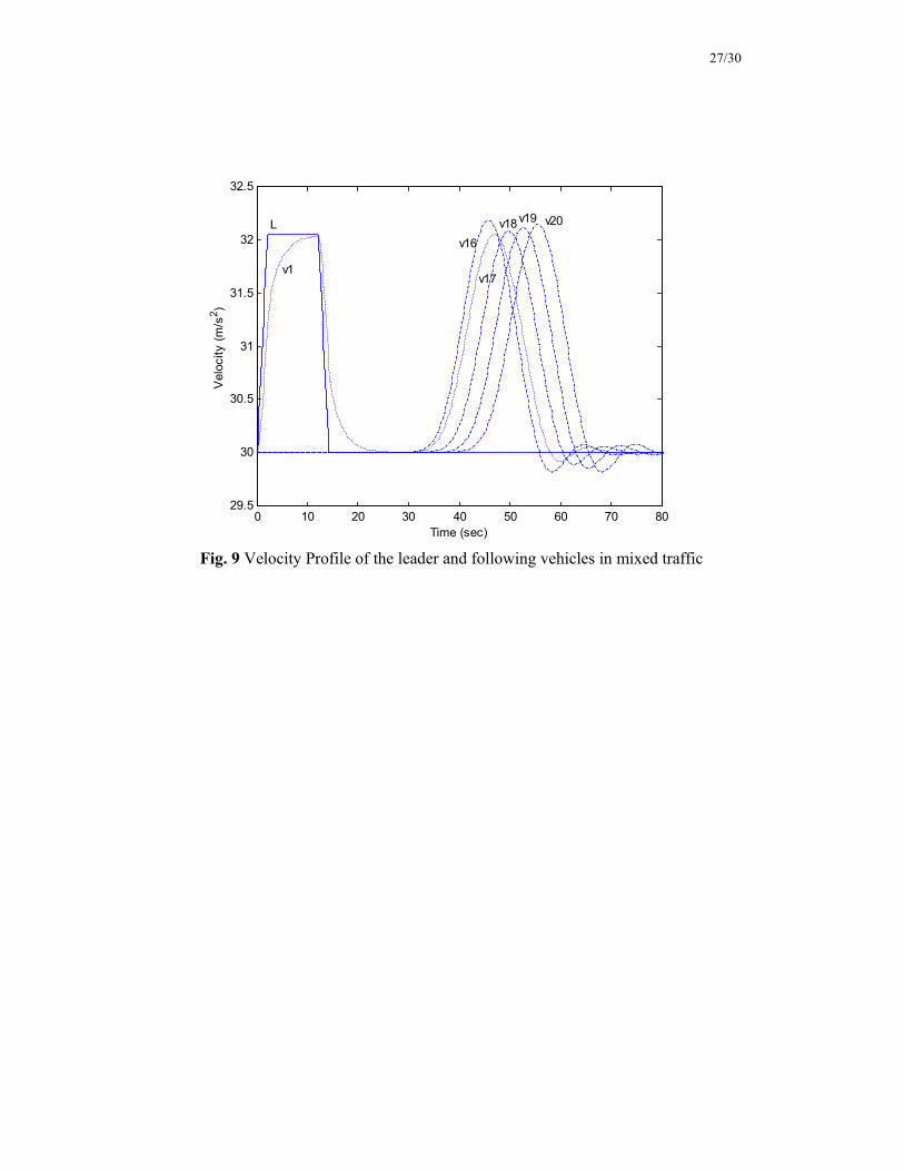
We then consider mixed manual/ACC vehicle strings. Assuming a mixed

string of 25% ACC vehicles, we investigate the identical situation when 20 vehicles

(manual/ACC) follow a lead vehicle in a single lane. The lead vehicle is given the

same maneuver as in previous case. The ACC vehicles are placed uniformly at

position 1, 5, 9, 13, and 17. The manual vehicles amplify the velocity errors as seen

earlier. However, the ACC vehicles successfully reduce the slinky effect caused by

manual vehicles (Fig. 9,10). As a result, the last vehicle (v20) shows a smaller

velocity change (compare with v16).

5.2 UMACC Study

In the UMACC simulation study, the movement of vehicles on a 20 km two-

lane test track are simulated for one hour. The results for different traffic densities

and different ACC penetration rates are shown in Table 2. For each selection of

traffic density and penetration rate, the average velocity, RMS value of acceleration,

and RMS value of range rate of all vehicles are calculated. It can be seen that at low

traffic density (7.5 veh/ln/km), the effect of ACC vehicles on traffic is not obvious.

As traffic density increases, the effect of ACC vehicles becomes more and more

profound. At high traffic density (20 veh/ln/km), for 40% ACC penetration rate, the

average velocity increases by 16%, the RMS of acceleration decreases by 27%, and

the RMS of range rate decreases by 37 %. The benefit of such an ACC system is

obvious. Higher average velocity means higher traffic throughput, lower RMS value

of acceleration means lower fuel consumption and lower air pollution, and lower

RMS value of range rate not only means smoother but also safer highway traffic.

Fig 7,8

Fig 9,10

Table 2

17/30

References

[1] Levine, W. and Athans, M.: On the Optimal Error Regulation of a String of

Moving Vehicles, IEEE Trans. Automat. Contr., vol. 11, no. 3, July, pp. 355-361

(1966).

[2] Liang, C. and Peng, H.: Optimal Adaptive Cruise Control with Guaranteed String

Stability, Proceedings of the 1998 AVEC Conference, Nagoya, Japan,

September, pp.717-722 (1998).

[3] Liang, C. and Peng, H.: Design and Simulations of A Traffic-Friendly Adaptive

Cruise Control Algorithm, Proceedings of the 1998 ASME International

Congress and Exposition, Anaheim, CA, November 1998.

[4] Caudill, R. J. and Garrard, W. L.: Vehicle-Follower Longitudinal Control for

Automated Transit Vehicles, J. of Dynamic Systems, Measurement, and Control,

December, pp. 241-248 (1977).

[5] Ioannou, P. and Chien, C.C.: Autonomous Intelligent Cruise Control, IEEE

Trans. Veh. Tech., Vol.42, No. 4, p. 657-672 (1993).

[6] Sheikholeslam, S. and Desoer, C. A.: Longitudinal Control of a Platoon of

Vehicles, Proc. of 1990 American Control Conference, San Diego, pp. 291-296

(1990).

[7] YanaKiev, D., Kanellakopoulos, I.: A Simplified Framework for String Stability

Analysis in AHS, Proc. of the 13th IFAC World Congress, Volume Q, pp.177-

182 (1996).

[8] Swaroop, D., Hedrick, J.K.: String Stability of Interconnected Systems, IEEE

Trans. Automat. Contr., vol. 41, no. 3, pp. 349-356 (1996).

18/30

[9] Fancher, P.S., Bareket, Z., Sayer, J.R., MacAdam, C., Ervin, R.D., Mefford,

M.L., Haugen, J.: Fostering Development, Evaluation, and Deployment of

Forward Crash Avoidance Systems (FOCAS), ARR-12-15-96, University of

Michigan Transportation Research Institute technical Report number 96-44

(1996).

[10] Chandler, R.E., Herman, R., and Montroll, E.W.: Traffic Dynamics: Studies in

Car Following, Operation Research, Vol. 6, p.165-184 (1958).

[11] Chu, K. C.: Optimal Decentralized Regulation for a String of Coupled Systems,

IEEE Trans. Automat. Contr., vol. 19, no. 3, pp. 243-246 (1974).

[12] Pipes, L.A.: An Operational Analysis of Traffic Dynamics, Journal of Applied

Physics, vol.24, pp. 274-281 (1953)

19/30

Vehicle interactions(R, R and lane calculations)

Drivermodel

Sensormodel

ACCAlgorithm

Vehicle model

Vehicle and driverprobability distributions Graphical

UserInterface

.

Fig. 1 ACC Simulator

20/30

Fig. 2 Probability of a Vehicle in platoons of Different Sizes

0

10

20

30

40

50

60

70

1 2 3 4 5 6 7 8 9 10Platoon Size (Veh)

Prob

abili

ty (%

)

2.5 Veh/Ln/Km7.5 Veh/Ln/Km12.5 Veh/Ln/Km17.5 Veh/Ln/Km

21/30

Fig. 3 Probability of a Vehicle in Platoons of Size > 10

0

5

10

15

20

25

30

35

40

45

2.5 3.75 5 6.25 7.5 8.75 10 11.3 12.5 13.8 15 16.3 17.5

Traffic Density (Veh/Ln/Km)

Prob

abili

ty (%

)

22/30

Fig. 4 Vehicle String

dk, dk dk+1, vk+1 dk-1, vk-1 dk+2, vk+2

23/30

Fig. 5 Mixed Vehicle String

x1, v1 x2, v2 xL, vL x3, v3

24/30

Fig. 6 Infinite Mixed Vehicle String

xL, vL xk+1,vk+1 xk, vk x1, v1 x2k, v2k

Sub-String (S2)

Sub-String (S1) Lead Vehicle

x2k+1,v2k+1

S3, S4, …

25/30

0 10 20 30 40 50 60 70 80 90 10028.5

29

29.5

30

30.5

31

31.5

32

32.5

33

33.5

Time (sec)

Vel

ocity

(m/s

)

Lv1

v18 v20

Fig. 7 Velocity profile of the leader and following vehicles

26/30

35

45

55

65

75

85

95

1 2 3 4 5 6 7 8 9 10 11 12 13 14 15 16 17 18 19 20Car #

SUM

((v-v

0)^2

*dt)

Fig. 8 2-Norm of (v-v0) of the following vehicles

27/30

Fig. 9 Velocity Profile of the leader and following vehicles in mixed traffic

0 10 20 30 40 50 60 70 8029.5

30

30.5

31

31.5

32

32.5

Time (sec)

Vel

ocity

(m/s

2 )L

v1

v16

v17

v18v19 v20

28/30

35

37

39

41

43

45

47

1 2 3 4 5 6 7 8 9 10 11 12 13 14 15 16 17 18 19 20

Car #

SUM

((v-v

0)^2

*dt)

Fig. 10 2-Norm of (v-v0) of the following vehicles

29/30

Table 1 Optimal Control Gains and Corresponding SSM for h=1.4 sec

q1 q2 r K* SSM 1 1 1 [1.12, 1.70] 4.22

0.1 0.1 1 [0.45, 1.44] 4.80 0.1 10 1 [0.42, 2.15] 4.86 10 0.1 1 [2.20, 2.47] 4.05 10 10 1 [2.10, 2.94] 4.70

30/30

Table 2 Effects of the optimal ACC systems under different traffic densities

ACC Penetration Rate 0% 20% 40% 60% 90%

V_avg (m/s) 27.75 27.70 27.71 27.58 27.57

RMS_a (m/s^2) 0.25 0.27 0.29 0.29 0.32 7.5

veh/km/ln

RMS_Rd (m/s) 2.26 2.25 2.28 2.17 2.20

V_avg (m/s) 25.85 25.42 25.67 25.78 25.72

RMS_a (m/s^2) 0.35 0.35 0.30 0.27 0.26 16.25 veh/km/ln

RMS_Rd (m/s) 1.93 1.90 1.58 1.47 1.35

V_avg (m/s) 20.19 21.15 23.38 24.64 24.65

RMS_a (m/s^2) 0.56 0.53 0.41 0.32 0.17 20

veh/km/ln

RMS_Rd (m/s) 3.31 3.08 2.08 1.34 0.70