Stretched exponential estimate on growth of the number of

periodic points for prevalent diffeomorphisms

Vadim Yu. Kaloshin1, Brian R. Hunt2

1 Mathematics 253-37, Caltech, Pasadena, CA 91125;

e-mail: kaloshin@its.caltech.edu

2 Department of Mathematics, Mathematics Building, University of Maryland

College Park, MD 20742-4015;

e-mail: bhunt@math.umd.edu

Abstract

For diffeomorphisms of smooth compact finite-dimensional manifolds, we consider

the problem of how fast the number of periodic points with period n grows as a

function of n. In many familiar cases (e.g., Anosov systems) the growth is expo-

nential, but arbitrarily fast growth is possible; in fact, the first author has shown

that arbitrarily fast growth is topologically (Baire) generic for C2 or smoother diffeo-

morphisms. In the present work we show that, by contrast, for a measure-theoretic

notion of genericity we call “prevalence”, the growth is not much faster than exponen-

tial. Specifically, we show that for each ρ, δ > 0, there is a prevalent set of C1+ρ (or

smoother) diffeomorphisms for which the number of period n points is bounded above

by exp(Cn1+δ) for some C independent of n. We also obtain a related bound on the

decay of hyperbolicity of the periodic points as a function of n, and obtain the same

results for 1-dimensional endomorphisms. The contrast between topologically generic

and measure-theoretically generic behavior for the growth of the number of periodic

points and the decay of their hyperbolicity shows this to be a subtle and complex

phenomenon, reminiscent of KAM theory. Here in Part I we state our results and

describe the methods we use. We complete most of the proof in the 1-dimensional

C2-smooth case and outline the remaining steps, deferred to Part II, that are needed

to establish the general case.

The novel feature of the approach we develop in this paper is the introduction

of Newton Interpolation Polynomials as a tool for perturbing trajectories of iterated

maps.

Table of Contents

1 A Problem of the Growth of the Number of Periodic Points and

Decay of Hyperbolicity for Generic Diffeomorphisms. 1

1.1 Introduction . . . . . . . . . . . . . . . . . . . . . . . . . . . . . . . . 1

1.2 Prevalence in the space of diffeomorphisms Diffr(M) . . . . . . . 5

1.3 Formulation of the main result in the multidimensional case . . . . . 7

1.4 Formulation of the main result in the 1–dimensional case . . . . . . . 10

2 Strategy of the Proof 13

2.1 Various perturbations of recurrent trajectories by Newton interpolation

polynomials . . . . . . . . . . . . . . . . . . . . . . . . . . . . . . . . 15

2.2 Newton interpolation and blow-up along the diagonal in multijet space 17

2.3 Estimates of the measure of “bad” parameters and Fubini reduction to

finite-dimensional families . . . . . . . . . . . . . . . . . . . . . . . . 22

2.4 Simple trajectories and the Inductive Hypothesis . . . . . . . . . . . 24

3 A Model Problem: C2-smooth Maps of the Interval I = [−1, 1] 29

3.1 Setting up of the model . . . . . . . . . . . . . . . . . . . . . . . . . . 29

3.2 Decomposition into pseudotrajectories . . . . . . . . . . . . . . . . . 32

3.3 Application of Newton interpolation polynomials to estimate the mea-

sure of “bad” parameters for a single trajectory . . . . . . . . . . . . 36

3.4 The Distortion and Collection Lemmas . . . . . . . . . . . . . . . . . 39

3.5 Discretization Method for trajectories with a gap . . . . . . . . . . . 45

3.5.1 Decomposition of nonsimple parameters into groups . . . . . . 52

3.5.2 Decomposition into i-th recurrent pseudotrajectories . . . . . . 54

3.6 The measure of maps fε having i-th recurrent, non sufficiently hyper-

bolic trajectories with a gap and proofs of auxiliary lemmas . . . . . 56

i

4 Comparison of the Discretization Method in 1–dimensional and N–

dimensional Cases 62

4.1 Dependence of the main estimates on N and ρ . . . . . . . . . . . . . 62

4.2 The multidimensional space of divided differences and dynamically es-

sential parameters . . . . . . . . . . . . . . . . . . . . . . . . . . . . . 63

4.3 The multidimensional Distortion Lemma . . . . . . . . . . . . . . . . 66

4.4 From a brick of at most standard thickness to an admissible brick . . 70

4.5 The main estimate on the measure of “bad” parameters . . . . . . . . 72

References 91

ii

Chapter 1

A Problem of the Growth of the

Number of Periodic Points and

Decay of Hyperbolicity for Generic

Diffeomorphisms.

1.1 Introduction

Let Diffr(M) be the space of Cr diffeomorphisms of a finite-dimensional smooth

compact manifold M with the uniform Cr–topology, where dimM ≥ 2, and let

f ∈ Diffr(M). Consider the number of periodic points of period n

Pn(f) = #{x ∈ M : x = fn(x)}. (1.1)

The main question of this paper is:

Question 1.1.1. How quickly can Pn(f) grow with n for a “generic” Cr diffeomor-

phism f?

We put the word “generic” in brackets because as the reader will see the answer

depends on notion of genericity.

For technical reasons one sometimes counts only isolated points of period n; let

P in(f) = #{x ∈ M : x = fn(x) and y 6= fn(y)

for y 6= x in some neighborhood of x}.(1.2)

1

We call a diffeomorphism f ∈ Diffr(M) an Artin-Mazur diffeomorphism (or simply

A-M diffeomorphism) if the number of isolated periodic orbits of f grows at most

exponentially fast, i.e. for some number C > 0 we have

P in(f) ≤ exp(Cn) for all n ∈ Z+. (1.3)

Artin & Mazur [AM] proved the following result.

Theorem 1.1.2. For 0 ≤ r ≤ ∞, A-M diffeomorphisms are dense in Diffr(M) with

the uniform Cr–topology.

We say that a point x ∈ M of period n for f is hyperbolic if dfn(x), the lineariza-

tion of fn at x, has no eigenvalues with modulus 1. (Notice that a hyperbolic solution

to fn(x) = x must also be isolated.) We call f ∈ Diffr(M) a strongly Artin-Mazur

diffeomorphism if for some number C > 0,

Pn(f) ≤ exp(Cn) for all n ∈ Z+, (1.4)

and all periodic points of f are hyperbolic (whence Pn(f) = P in(f)). In [K1] an

elementary proof of the following extension of the Artin-Mazur result is given.

Theorem 1.1.3. For 0 ≤ r < ∞, strongly A-M diffeomorphisms are dense in

Diffr(M) with the uniform Cr–topology.

According to the standard terminology a set in Diffr(M) is called residual if it

contains a countable intersection of open dense sets and a property is called (Baire)

generic if diffeomorphisms with that property form a residual set. It turns out the

A-M property is not generic, as is shown in [K2]. Moreover:

Theorem 1.1.4. [K2] For any 2 ≤ r < ∞ there is an open set N ⊂ Diffr(M)

such that for any given sequence a = {an}n∈Z+ there is a Baire generic set Ra in Ndepending on the sequence an with the property if f ∈ Ra, then for infinitely many

nk ∈ Z+ we have P ink

(f) > ank.

Of course since Pn(f) ≥ P in(f), the same statement can be made about Pn(f). But

in fact it is shown in [K2] that Pn(f) is infinite for n sufficiently large, due to a

continuum of periodic points, for at least a dense set of f ∈ N .

The proof of this Theorem is based on a result of Gonchenko-Shilnikov-Turaev

[GST1]. Two slightly different detailed proofs of their result are given in [K2] and

[GST2]. The proof in [K2] relies on a strategy outlined in [GST1].

2

However, it seems unnatural that if you pick a diffeomorphism at random then

it may have an arbitrarily fast growth of number of periodic points. Moreover, Baire

generic sets in Euclidean spaces can have zero Lebesgue measure. Phenomena that

are Baire generic, but have a small probability are well-known in dynamical systems,

KAM theory, number theory, etc. (see [O], [HSY], [K3] for various examples). This

partially motivates the problem posed by Arnold [A]:

Problem 1.1.5. Prove that “with probability one” f ∈ Diffr(M) is an A-M diffeo-

morphism.

Arnold suggested the following interpretation of “with probability one”: for a

(Baire) generic finite parameter family of diffeomorphisms {fε}, for Lebesgue almost

every ε we have that fε is A-M (compare with [K3]). As Theorem 1.3 shows, a result

on the genericity of the set of A-M diffeomorphisms based on (Baire) topology is likely

to be extremely subtle, if possible at all 1. We use instead a notion of “probability

one” based on prevalence [HSY, K3], which is independent of Baire genericity. We

also are able to state the result in the form Arnold suggested for generic families using

this measure-theoretic notion of genericity.

For a rough understanding of prevalence, consider a Borel measure µ on a Banach

space V . We say that a property holds “µ–almost surely for perturbations” if it holds

on a Borel set P ⊂ V such that for all v ∈ V we have v + w ∈ P for almost

every w with respect to µ. Notice that if V = Rk and µ is Lebesgue measure, then

“almost surely with respect to perturbations by µ” is equivalent to “Lebesgue almost

everywhere”. Moreover, the Fubini/Tonelli Theorem implies that if µ is any Borel

probability measure on Rk, then a property that holds almost surely with respect

to perturbations by µ must also be hold Lebesgue almost everywhere. Based on this

observation, we call a property on a Banach space “prevalent” if it holds almost surely

with respect to perturbations by µ for some Borel probability measure µ on V , which

for technical reasons we require to have compact support. In order to apply this notion

to the Banach manifold Diffr(M), we must describe how we make perturbations in

this space, which we will do in the next Section.

Our first main result is a partial solution to Arnold’s problem. It says that for

a prevalent diffeomorphism f ∈ Diffr(M), with 1 < r ≤ ∞, and all δ > 0 there exists

1For example, using technique from [GST2] and [K2] one can prove that for a (Baire) generic finite-

parameter family {fε} and a (Baire) generic parameter value ε the corresponding diffeomorphism fε

is not A-M. Unfortunately, how to estimate the measure of non-A-M diffeomorphisms from below is

a so far unreachable question

3

C = C(δ) > 0 such that for all n ∈ Z+,

Pn(f) ≤ exp(Cn1+δ). (1.5)

The results of this paper have been announced in [KH].

The Kupka-Smale Theorem (see e.g.[PM]) states that for a generic diffeomor-

phism all periodic points are hyperbolic and all associated stable and unstable mani-

folds intersect one another transversally. [K3] shows that the Kupka-Smale Theorem

also holds on a prevalent set. So, the Kupka-Smale Theorem, in particular, says that

a Baire generic (resp. prevalent) diffeomorphism has only hyperbolic periodic points,

but how hyperbolic are the periodic points, as function of their period, for a Baire

generic (resp. prevalent) diffeomorphism f? This is the second main problem we

deal with in this paper.

Recall that a linear operator L : RN → R

N is hyperbolic if it has no eigenvalues

on the unit circle {|z| = 1} ⊂ C. Denote by | · | the Euclidean norm in CN . Then we

define the hyperbolicity of a linear operator L by

γ(L) = infφ∈[0,1)

inf|v|=1

|Lv − exp(2πiφ)v|. (1.6)

We also say that L is γ–hyperbolic if γ(L) ≥ γ. In particular, if L is γ–hyperbolic,

then its eigenvalues {λj}Nj=1 ⊂ C are at least γ–distant from the unit circle, i.e.

minj ||λj| − 1| ≥ γ. The hyperbolicity of a periodic point x = fn(x) of period n,

denoted by γn(x, f), equals the hyperbolicity of the linearization dfn(x) of fn at

points x, i.e. γn(x, f) = γ(dfn(x)). Similarly the number of periodic points Pn(f) of

period n is defined, one can define

γn(f) = min{x: x=fn(x)}

γn(x, f). (1.7)

The idea of Gromov [G] and Yomdin [Y] of measuring hyperbolicity is that a γ–

hyperbolic point of period n of a C2 diffeomorphism f has an M−2n2 γ–neighborhood

(where M2 = ‖f‖C2) free from periodic points of the same period2. In Appendix A

we prove the following result.

Proposition 1.1.6. Let M be a compact manifold of dimension N , let f : M → M

be a C1+ρ diffeomorphism, where 0 < ρ ≤ 1, that has only hyperbolic periodic points,

2In [Y] hyperbolicity is introduced as the minimal distance of eigenvalues to the unit circle. This

way of defining hyperbolicity does not guarantee the existence of a M−2n2 γ–neighborhood free from

periodic points of the same period; see Appendix A.

4

and let M1+ρ = max{‖f‖C1+ρ , 21/ρ}. Then there is a constant C = C(M) > 0 such

that for each n ∈ Z+ we have

Pn(f) ≤ C (M1+ρ)nN(1+ρ)/ρ γn(f)−N/ρ. (1.8)

Proposition 1.1.6 implies that a lower estimate on a decay of hyperbolicity γn(f)

gives an upper estimate on growth of number of periodic points Pn(f). Therefore, a

natural question is:

Question 1.1.7. How quickly can γn(f) decay with n for a “generic” Cr diffeomor-

phism f?

For a Baire generic f ∈ Diffr(M), the existence of lower bound on a rate of

decay of γn(f) would imply the existence of an upper bound on a rate of growth of

the number of periodic points Pn(f), whereas no such bound exists by Theorem 1.1.4.

Thus again we consider genericity in the measure-theoretic sense of prevalence. Our

second main result, which in view of Proposition 1.1.6 implies the first main result,

is that for a prevalent diffeomorphism f ∈ Diffr(M), with 1 < r ≤ ∞, and for any

δ > 0 there exists C = C(δ) > 0 such that

γn(f) ≥ exp(−Cn1+δ). (1.9)

Now we shall discuss in more detail our definition of prevalence (“probability

one”) in the space of diffeomorphisms Diffr(M).

1.2 Prevalence in the space of diffeomorphisms

Diffr(M)

The space of Cr diffeomorphisms Diffr(M) of a compact manifold M is a Banach

manifold. Locally we can identify it with a Banach space, which gives it a local lin-

ear structure in the sense that we can perturb a diffeomorphism by “adding” small

elements of the Banach space. As we described in the previous Section, the notion of

prevalence requires us to make additive perturbations with respect to a probability

measure that is independent of the place where we make the perturbation. Thus al-

though there is not a unique way to put a linear structure on Diffr(M), it is important

to make a choice that is consistent throughout the Banach manifold.

The way we make perturbations on Diffr(M) by small elements of a Banach space

is as follows. First we embed M into the interior of the closed unit ball BN ⊂ RN ,

5

which we can do for N sufficiently large by the Whitney Embedding Theorem [W].

We emphasize that our results hold for every possible choice of an embedding of

M into RN . We then consider a closed neighborhood U ⊂ BN of M and Banach

space Cr(U, RN) of Cr functions from U to RN . Next we extend every element f ∈

Diffr(M) to an element F ∈ Cr(U, RN) that is strongly contracting in all the directions

transverse to M3. Again the particular choice of how we make this extension is not

important to our results; in Appendix C we describe how to extend a diffeomorphism

and what conditions we need to ensure that the results of Sacker [Sac] and Fenichel

[F] apply as follows. Since F has M as an invariant manifold, if we add to F a small

perturbation in g ∈ Cr(U, RN), the perturbed map F +g has an invariant manifold in

U that is Cr-close to M . Then F + g restricted to its invariant manifold corresponds

in a natural way to an element of Diffr(M), which we consider to be the perturbation

of f ∈ Diffr(M) by g ∈ Cr(U, RN). The details of this construction are described in

Appendix C.

In this way we reduce the problem to the study of maps in Diffr(U), the open

subset of Cr(U, RN) consisting of those elements that are diffeomorphisms from U to

some subset of its interior. The construction we described in the previous paragraph

ensures that the number of periodic points Pn(f) and their hyperbolicity γn(f) for

elements of Diffr(M) are the same for the corresponding elements of Diffr(U), so

the bounds that we prove on these quantities for almost every perturbation of any

element of Diffr(U) hold as well for almost every perturbation of any element of

Diffr(M). Another justification for considering diffeomorphisms in Euclidean space is

that the problem of exponential/superexponential growth of the number of periodic

points Pn(f) for a prevalent f ∈ Diffr(M) is a local problem on M and is not affected

by a global shape of M .

The results stated in the next Section apply to any compact domain U ⊂ RN ,

but for simplicity we state them for the closed unit ball BN . In the previous Section,

we said that a property is prevalent on a Banach space such as Cr(BN) if it holds

on a Borel subset S for which there exists a Borel probability measure µ on Cr(BN)

with compact support such that for all f ∈ Cr(BN) we have f + g ∈ S for almost

every g with respect to µ. The complement of a prevalent set is said to be shy . We

then say that a property is prevalent on an open subset of Cr(BN) such as Diffr(BN)

if the exceptions to the property in Diffr(BN) form a shy subset of Cr(BN).

In this paper the perturbation measure µ that we use is supported within the

analytic functions in Cr(BN). In this sense we foliate Diffr(BN) by analytic leaves

3The existence of such an extension is not obvious, as pointed out by C. Carminati.

6

that are compact and overlapping. The main result then says that for every analytic

leaf L ⊂ Diffr(BN) and every δ > 0, for almost every diffeomorphism f ∈ L in the

leaf L both (1.5) and (1.9) are satisfied. Now we define an analytic leaf as a “Hilbert

Brick” in the space of analytic functions and a natural Lebesgue product probability

measure µ on it.

1.3 Formulation of the main result in the multidi-

mensional case

Fix a coordinate system x = (x1, . . . , xN) ∈ RN ⊃ BN and the scalar product 〈x, y〉 =

∑

i xiyi. Let α = (α1, . . . , αN) be a multiindex from ZN+ , and let |α| =

∑

i αi. For a

point x = (x1, . . . , xN) ∈ RN we write xα =

∏Ni=1 xαi

i . Associate to a real analytic

function φ : BN → RN the set of coefficients of its expansion:

φ~ε(x) =∑

α∈ZN+

~εαxα. (1.10)

Denote by Wk,N the space of N–component homogeneous vector-polynomials of de-

gree k in N variables and by ν(k,N) = dim Wk,N the dimension of Wk,N . According

to the notation of the expansion (1.10), denote coordinates in Wk,N by

~εk =({~εα}|α|=k

)∈ Wk,N . (1.11)

In Wk,N we use a scalar product that is invariant with respect to orthogonal trans-

formation of RN ⊃ BN (see Appendix B), defined as follows:

〈~εk, ~νk〉k =∑

|α|=k

(k

α

)−1

〈~εα, ~να〉, ‖~εk‖k =(〈~εk, ~εk〉k

)1/2. (1.12)

Denote by

BNk (r) = {~εk ∈ Wk,N : ‖~εk‖k ≤ r} (1.13)

the closed r–ball in Wk,N centered at the origin. Let Lebk,N be Lebesgue measure on

Wk,N induced by the scalar product (1.12) and normalized by a constant so that the

volume of the unit ball is one: Lebk,N(BNk (1)) = 1.

7

Fix a nonincreasing sequence of positive numbers ~r = ({rk}∞k=0) such that rk → 0

as k → ∞ and define a Hilbert Brick of size ~r

HBN(~r) ={~ε = {~εα}α∈ZN+

: for all k ∈ Z+, ‖~εk‖k ≤ rk}=BN

0 (r0) × BN1 (r1) × · · · × BN

k (rk) × . . .

⊂ W0,N × W1,N × · · · × Wk,N × . . . .

(1.14)

Define a Lebesgue product probability measure µN~r associated to the Hilbert Brick

HBN(~r) of size ~r by normalizing for each k ∈ Z+ the corresponding Lebesgue measure

Lebk,N on Wk,N to the Lebesgue probability measure on the rk–ball BNk (rk):

µNk,r = r−ν(k,N) Lebk,N and µN

~r = ×∞k=0µ

Nk,rk

. (1.15)

Definition 1.3.1. Let f ∈ Diffr(BN) be a Cr diffeomorphism of BN into its interior.

We call HBN(~r) a Hilbert Brick of an admissible size ~r = ({rk}∞k=0) with respect to

f if

A) for each ~ε ∈ HBN(~r), the corresponding function φ~ε(x) =∑

α∈ZN+

~εαxα is analytic

on BN ;

B) for each ~ε ∈ HBN(~r), the corresponding map f~ε(x) = f(x)+φ~ε(x) is a diffeomor-

phism from BN into its interior, i.e. {f~ε}~ε∈HBN (~r) ⊂ Diffr(BN);

C) for all δ > 0 and all C > 0, the sequence rk exp(Ck1+δ) → ∞ as k → ∞.

Remark 1.3.2. The first and second conditions ensure that the family {f~ε}~ε∈HBN (~r)

lie inside an analytic leaf within the class of diffeomorphisms Diffr(BN). The third

condition provides us enough freedom to perturb. It is important for our method to

have infinitely many parameters to perturb. If rk’s were decaying too fast to zero it

would make our family of perturbations essentially finite-dimensional.

An example of an admissible sequence ~r = ({rk}∞k=0) is rk = τ/k!, where τ

depends on f and is chosen sufficiently small to ensure that condition (B) holds.

Notice that the diameter of HBN(~r) is then proportional to τ , so that τ can be

chosen as some multiple of the distance from f to the boundary of Diffr(BN).

Main Theorem. For any 0 < ρ ≤ ∞ (or even 1 + ρ = ω) and any C1+ρ diffeomor-

phism f ∈ Diff1+ρ(BN), consider a Hilbert Brick HBN(~r) of an admissible size ~r with

respect to f and the family of analytic perturbations of f

{f~ε(x) = f(x) + φ~ε(x)}~ε∈HBN (~r) (1.16)

with the Lebesgue product probability measure µN~r associated to HBN(~r). Then for

every δ > 0 and µN~r –a.e. ~ε there is C = C(~ε, δ) > 0 such that for all n ∈ Z+

γn(f~ε) > exp(−Cn1+δ), Pn(f~ε) < exp(Cn1+δ). (1.17)

8

Remark 1.3.3. The fact that the measure µN~r depends on f does not conform to

our definition of prevalence. However, we can decompose Diffr(BN) into a nested

countable union of sets Sj that are each a positive distance from the boundary of

Diffr(BN) and for each j ∈ Z+ choose an admissible sequence ~rj that is valid for

all f ∈ Sj. Since a countable intersection of prevalent subsets of a Banach space is

prevalent [HSY], the Main Theorem implies the results stated in terms of prevalence

in the introduction.

Remark 1.3.4. Recently the first author along with A. Gorodetski [GK] applied the

technique developed here and obtained partial solution of Palis’ conjecture about finite-

ness of the number of coexisting sinks for surface diffeomorphisms.

In Appendix C we deduce from the Main Theorem the following result.

Theorem 1.3.5. Let {fε}ε∈Bm ⊂ Diff1+ρ(M) be a generic m–parameter family of

C1+ρ diffeomorphisms of a compact manifold M for some ρ > 0. Then for every

δ > 0 and a.e. ε ∈ Bm there is a constant C = C(ε, δ) such that (1.17) is satisfied

for every n ∈ Z+.

In Appendix C we also give a precise meaning to the term generic. Now we formulate

the most general result we shall prove.

Definition 1.3.6. Let γ ≥ 0 and f ∈ Diff1+ρ(BN) be a C1+ρ diffeomorphism for some

ρ > 0. A point x ∈ BN is called (n, γ)–periodic if |fn(x)−x| ≤ γ and (n, γ)–hyperbolic

if γn(x, f) = γ(dfn(x)) ≥ γ.

(Notice that a point can be (n, γ)–hyperbolic regardless of its periodicity, but this

property is of interest primarily for (n, γ)–periodic points.) For positive C and δ let

γn(C, δ) = exp(−Cn1+δ).

Theorem 1.3.7. Given the hypotheses of the Main Theorem, for every δ > 0 and for

µN~r –a.e. ~ε there is C = C(~ε, δ) > 0 such that for all n ∈ Z+, every (n, γ

1/ρn (C, δ))–

periodic point x ∈ BN is (n, γn(C, δ))–hyperbolic. (Here we assume 0 < ρ ≤ 1; in a

space Diff1+ρ(BN) with ρ > 1, the statement holds with ρ replaced by 1.)

This result together with Proposition 1.1.6 implies the Main Theorem, because any

periodic point of period n is (n, γ)–periodic for any γ > 0.

Remark 1.3.8. In the statement of the Main Theorem and Theorem 1.3.7 the unit

ball BN can be replaced by an bounded open set U ⊂ RN . After scaling U can be

considered as a subset of the unit ball BN .

9

One can define a distance on a compact manifold M and almost periodic points

of diffeomorphisms of M . Then one can cover M = ∪iUi by coordinate charts and

define hyperbolicity for almost periodic points using these charts {Ui}i (see [Y] for

details). This gives a precise meaning to the following result.

Theorem 1.3.9. Let {fε}ε∈Bm ⊂ Diff1+ρ(M) be a generic m–parameter family of

diffeomorphisms of a compact manifold M for some ρ > 0. Then for every δ > 0 and

almost every ε ∈ Bm there is a constant C = C(ε, δ) such that every (n, γ1/ρn (C, δ))–

periodic point x in BN is (n, γn(C, δ))–hyperbolic. (Here again we assume 0 < ρ ≤ 1,

replacing ρ with 1 in the conclusion if ρ > 1.)

The meaning of the term generic is the same as in Theorem 1.3.5 and is discussed

in Appendix C.

1.4 Formulation of the main result in the 1–dimen-

sional case

The proof of the main multidimensional result (Theorem 1.3.7) is quite long and

complicated. In order to describe the general approach we develop in this paper we

apply our method to the 1–dimensional maps which represent a nontrivial simplified

model for the multidimensional problem. The statement of the main result for the

1–dimensional maps has another important feature: it clarifies the statement of the

main multidimensional result.

Fix the interval I = [−1, 1]. Associate to a real analytic function φ : I → R the

set of coefficients of its expansion

φε(x) =∞∑

k=0

εkxk. (1.18)

For a nonincreasing sequence of positive numbers ~r = ({rk}∞k=0) such that rk → 0 as

k → ∞ following the multidimensional notations we define a Hilbert Brick of size ~r

HB1(~r) = {ε = {εk}∞k=0 : for all k ∈ Z+, |εk| ≤ rk} (1.19)

and the product probability measure µ1~r associated to the Hilbert Brick HB1(~r) of

size ~r which considers each εk as a random variable uniformly distributed on [−rk, rk]

and independent from the other εk’s.

10

Main 1–dimensional Theorem. For any 0 < ρ ≤ ∞ (or even 1 + ρ = ω) and any

C1+ρ map f : I → I of the interval I = [−1, 1] consider a Hilbert Brick HB1(~r) of

an admissible size ~r with respect to f and the family of analytic perturbations of f

{fε(x) = f(x) + φε(x)}ε∈HB1(~r) (1.20)

with the Lebesgue product probability measure µ1~r associated to HB1(~r). Then for

every δ > 0 and µ1~r–a.e. ε there is C = C(ε, δ) > 0 such that for all n ∈ Z+

γn(fε) > exp(−Cn1+δ), Pn(fε) < exp(Cn1+δ). (1.21)

Moreover, for µ1~r–a.e. ε, every (n, exp(−Cn1+δ))–periodic point is (n, exp(−Cn1+δ))–

hyperbolic.

In [MMS] Martens-de Melo-Van Strien prove a stronger statement for C2 maps.

They show that for any C2 map f of an interval without flat critical points there are

γ > 0 and n0 ∈ Z+ such that for any n > n0 we have |γn(f)| > 1 + γ. This also

implies that the number of periodic points is bounded by an exponential function of

the period. The notion of a flat critical point used in [MMS] is a nonstandard one

from a point of view of singularity theory, in particular, if 0 is a critical point, then

distance of f(x) to f(0) does not have to decay to 0 as x → 0 faster than any degree

of x.

In [KK] an example of a Cr–unimodal map with a critical point having tangency

of order 2r + 2 and an arbitrary fast rate of growth of the number of periodic points

is presented.

Let us point out again that the main purpose of discussing the 1-dimensional case

in details is to highlight ideas and explain the general method without overloading

presentation by technical details. The general N -dimensional case is highly involved

and excessive amount of technical details make understanding of general ideas of the

method not easily accessible.

Acknowledgments: It is great pleasure to thank the thesis advisor of the first

author, John Mather, who regularly spent hours listening oral expositions of various

parts of the proof for nearly two years4. Without his patience and support this project

would have never been completed. The authors are truly grateful to Anton Gorodet-

ski, Giovanni Forni, and an anonymous referee who read the manuscript carefully and

have made many useful remarks. The first author is grateful to Anatole Katok for

providing an opportunity to give a minicourse on the subject of this paper at Penn

4This paper is based on the first author’s Ph.D. thesis.

11

State University during the fall of 2000. The authors have profited from conversa-

tions with Carlo Carminati, Bill Cowieson, Dima Dolgopyat, Anatole Katok, Michael

Lyubich, Michael Shub, Yakov Sinai, Marcelo Viana, Jean-Christophe Yoccoz, Lai-

Sang Young, and many others. The first author thanks the Institute for Physical

Science and Technology, University of Maryland and, in particular, James Yorke for

their hospitality. The second author is grateful in turn to the Institute for Advanced

Study at Princeton for its hospitality. The first author acknowledges the support of

Sloan dissertation fellowship during his final year at Princeton, when significant part

of the work had been done. The first author is supported by NSF-grant DMS-0300229

and the second author by NSF grant DMS-0104087.

12

Chapter 2

Strategy of the Proof

Here we describe the strategy of the proof of the Main Result (Theorem 1.3.7). The

general idea is to fix C > 0 and prove an upper bound on the measure of the set of

“bad” parameter values ~ε ∈ HBN(~r) for which the conclusion of the Theorem does

not hold. The upper bound we obtain will approach zero as C → ∞, from which it

follows immediately that the set of ~ε ∈ HBN(~r) that are “bad” for all C > 0 has

measure zero. For a given C > 0, we bound the measure of “bad” parameter values

inductively as follows.

Stage 1. We delete all parameter values ~ε ∈ HBN(~r) for which the corresponding

diffeomorphism f~ε has an almost fixed point which is not sufficiently hyperbolic and

bound the measure of the deleted set.

Stage 2. We consider only parameter values for which each almost fixed point

is sufficiently hyperbolic. Then we delete all parameter values ~ε for which f~ε has an

almost periodic point of period 2 which is not sufficiently hyperbolic and bound the

measure of that set.

Stage n. We consider only parameter values for which each almost periodic point

of period at most n − 1 is sufficiently hyperbolic (we shall call this the Inductive

Hypothesis). Then we delete all parameter values ~ε for which f~ε has an almost

periodic point of period n which is not sufficiently hyperbolic and bound the measure

of that set.

The main difficulty in the proof is then to prove a bound on the measure of

“bad” parameter values at stage n such that the bounds are summable over n and

that the sum approaches zero as C → ∞. Let us formalize the problem. Fix positive

ρ, δ, and C, and recall that γn(C, δ) = exp(−Cn1+δ) for n ∈ Z+. Assume ρ ≤ 1; if

not, change its value to 1.

13

Definition 2.0.1. A diffeomorphism f ∈ Diff1+ρ(BN) satisfies the Inductive Hypoth-

esis of order n with constants (C, δ, ρ), denoted f ∈ IH(n,C, δ, ρ), if for all k ≤ n,

every (k, γ1/ρk (C, δ))-periodic point is (k, γk(C, δ))-hyperbolic.

For f ∈ Diff1+ρ(M), consider the sequence of sets in the parameter space HBN(~r)

Bn(C, δ, ρ,~r, f) = {~ε ∈ HBN(~r) :

f~ε ∈ IH(n − 1, C, δ, ρ) but f~ε /∈ IH(n,C, δ, ρ)}(2.1)

In other words, Bn(C, δ, ρ,~r, f) is the set of “bad” parameter values ~ε ∈ HBN(~r) for

which all almost periodic points of f~ε with period strictly less than n are sufficiently

hyperbolic, but there is an almost periodic point of period n that is not sufficiently

hyperbolic. Let

M1 = sup~ε∈HBN (~r)

max{‖f~ε‖C1 , ‖f−1~ε ‖C1};

M1+ρ = sup~ε∈HBN (~r)

max{‖f~ε‖C1+ρ ,M1, 21/ρ}.

(2.2)

Our goal is to find an upper bound

µN~r {Bn(C, δ, ρ,~r, f)} ≤ µn(C, δ, ρ,~r,M1+ρ). (2.3)

for the measure of the set of “bad” parameter values. Then the sum over n of (2.3)

gives an upper bound

µN~r {∪∞

n=1Bn(C, δ, ρ,~r, f)} ≤∞∑

n=1

µn(C, δ, ρ,~r,M1+ρ) (2.4)

on the measure of the set of all parameters ~ε for which f~ε has for at least one n an

(n, γ1/ρn (C, δ))-periodic point that is not (n, γn(C, δ))-hyperbolic. If this sum converges

and

∞∑

n=1

µn(C, δ, ρ,~r,M1+ρ) = µ(C, δ, ρ,~r,M1+ρ) → 0 as C → ∞ (2.5)

for every positive ρ, δ, and M1+ρ, then Theorem 1.3.7 follows. In the remainder of this

Chapter we describe the key construction we use to obtain a bound µn(C, δ, ρ,~r,M1+ρ)

that meets condition (2.5).

14

2.1 Various perturbations of recurrent trajectories

by Newton interpolation polynomials

The approach we take to estimate the measure of “bad” parameter values in the

space of perturbations HBN(~r) is to choose a coordinate system for this space and

for a finite subset of the coordinates to estimate the amount that we must change

a particular coordinate to make a “bad” parameter value “good”. Actually we will

choose a coordinate system that depends on a particular point x0 ∈ BN , the idea

being to use this coordinate system to estimate the measure of “bad” parameter

values corresponding to initial conditions in some neighborhood of x0, then cover BN

with a finite number of such neighborhoods and sum the corresponding estimates.

For a particular set of initial conditions, a diffeomorphism will be “good” if every

point in the set is either sufficiently nonperiodic or sufficiently hyperbolic.

In order to keep the notations and formulas simple as we formalize this approach,

we consider the case of 1-dimensional maps, but the reader should always have in mind

that our approach is designed for multidimensional diffeomorphisms. Let f : I → I

be a C1 map on the interval I = [−1, 1]. Recall that a trajectory {xk}k∈Z of f is

called recurrent if it returns arbitrarily close to its initial position – that is, for all

γ > 0 we have |x0 − xn| < γ for some n > 0. A very basic question is how much one

should perturb f to make x0 periodic. Here is an elementary Closing Lemma that

gives a simple partial answer to this question.

Closing Lemma. Let {xk = fk(x0)}nk=0 be a trajectory of length n + 1 of a map

f : I → I. Let u = (x0 − xn)/∏n−2

k=0(xn−1 − xk). Then x0 is a periodic point of period

n of the map

fu(x) = f(x) + un−2∏

k=0

(x − xk) (2.6)

Of course fu is close to f if and only if u is sufficiently small, meaning that |x0 − xn|should be small compared to

∏n−2k=0 |xn−1 − xk|. However, this product is likely to

contain small factors for recurrent trajectories. In general, it is difficult to control the

effect of perturbations for recurrent trajectories. The simple reason why this is so is

because one can not perturb f at two nearby points independently .

The Closing Lemma above also gives an idea of how much we must change the

parameter u to make a point x0 that is (n, γ)-periodic not be (n, γ)-periodic for a

given γ > 0, which as we described above is one way to make a map that is “bad”

for the initial condition x0 become “good”. To make use of the other part of our

15

alternative we must determine how much we need to perturb a map f to make a

given x0 be (n, γ)-hyperbolic for some γ > 0.

Perturbation of hyperbolicity. Let {xk = fk(x0)}n−1k=0 be a trajectory of length n

of a C1 map f : I → I. Then for the map

fv(x) = f(x) + v(x − xn−1)n−2∏

k=0

(x − xk)2 (2.7)

such that v ∈ R and

||(fnv )′(x0)| − 1| =

∣∣∣∣∣

∣∣∣∣∣

n−1∏

k=0

f ′(xk) + v

n−2∏

k=0

(xn−1 − xk)2

n−2∏

k=0

f ′(xk)

∣∣∣∣∣− 1

∣∣∣∣∣> γ

(2.8)

we have that x0 is an (n, γ)-hyperbolic point of fv.

One more time we can see the product of distances∏n−2

k=0 |xn−1 − xk| along the

trajectory is an important quantitative characteristic of how much freedom we have

to perturb.

The perturbations (2.6) and (2.7) are reminiscent of Newton interpolation poly-

nomials. Let us put these formulas into a general setting using singularity theory.

Given n > 0 and a C1 function f : I → R we define an associated function

j1,nf : In → In × R2n by

j1,nf(x0, . . . , xn−1) =(

x0, . . . ,xn−1, f(x0), . . . , f(xn−1),

f ′(x0), . . . , f′(xn−1)

)

.(2.9)

In singularity theory this function is called the n-tuple 1-jet of f . The ordinary

1-jet of f , usually denoted by j1f(x) = (x, f(x), f ′(x)), maps I to the 1-jet space

J 1(I, R) ≃ I × R2. The product of n copies of J 1(I, R), called the multijet space, is

denoted by

J 1,n(I, R) = J 1(I, R) × · · · × J 1(I, R)︸ ︷︷ ︸

n times

, (2.10)

and is equivalent to In × R2n after rearranging coordinates. The n-tuple 1-jet of f

associates with each n-tuple of points in In all the information necessary to determine

how close the n-tuple is to being a periodic orbit, and if so, how close it is to being

nonhyperbolic.

16

The set

∆n(I) ={

{x0, . . . , xn−1} × In × Rn ⊂ J 1,n(I, R) :

∃ i 6= j such that xi = xj

} (2.11)

is called the diagonal (or sometimes the generalized diagonal) in the space of multijets.

In singularity theory the space of multijets is defined outside of the diagonal ∆n(I)

and is usually denoted by J 1n (I, R) = J 1,n(I, R) \ ∆n(I) (see [GG]). It is easy to

see that a recurrent trajectory {xk}k∈Z+ is located in a neighborhood of the diagonal

∆n(I) ⊂ J 1,n(I, R) in the space of multijets for a sufficiently large n. If {xk}n−1k=0 is

a part of a recurrent trajectory of length n, then the product of distances along the

trajectory

n−2∏

k=0

|xn−1 − xk| (2.12)

measures how close {xk}n−1k=0 to the diagonal ∆n(I), or how independently one can

perturb points of a trajectory. One can also say that (2.12) is a quantitative charac-

teristic of how recurrent a trajectory of length n is. Introduction of this product of

distances along a trajectory into analysis of recurrent trajectories is a new point of

our paper.

2.2 Newton interpolation and blow-up along the

diagonal in multijet space

Now we present a construction due to Grigoriev and Yakovenko [GY] which puts

the “Closing Lemma” and “Perturbation of Hyperbolicity” statements above into

a general framework. It is an interpretation of Newton interpolation polynomials

as an algebraic blow-up along the diagonal in the multijet space. In order to keep

the notations and formulas simple we continue in this section to consider only the

1-dimensional case.

Consider the 2n-parameter family of perturbations of a C1 map f : I → I by

polynomials of degree 2n − 1

fε(x) = f(x) + φε(x), φε(x) =2n−1∑

k=0

εkxk, (2.13)

17

where ε = (ε0, . . . , ε2n−1) ∈ R2n. The perturbation vector ε consists of coordinates

from the Hilbert Brick HB1(~r) of analytic perturbations defined in Section 1.3. Our

goal now is to describe how such perturbations affect the n-tuple 1-jet of f , and since

the operator j1,n is linear in f , for the time being we consider only the perturbations

φε and their n-tuple 1-jets. For each n-tuple {xk}n−1k=0 there is a natural transformation

J 1,n : In × R2n → J 1,n(I, R) from ε-coordinates to jet-coordinates, given by

J 1,n(x0, . . . , xn−1, ε) = j1,nφε(x0, . . . , xn−1). (2.14)

Instead of working directly with the transformation J 1,n, we introduce interme-

diate u-coordinates based on Newton interpolation polynomials. The relation between

ε-coordinates and u-coordinates is given implicitly by

φε(x) =2n−1∑

k=0

εkxk =

2n−1∑

k=0

uk

k−1∏

j=0

(x − xj(mod n)). (2.15)

Based on this identity, we will define functions D1,n : In × R2n → In × R

2n and

π1,n : In × R2n → J 1,n(I, R) so that J 1,n = π1,n ◦ D1,n, or in other words the

diagram in Figure 1 commutes. We will show later that D1,n is invertible, while π1,n

is invertible away from the diagonal ∆n(I) and defines a blow-up along it in the space

of multijets J 1,n(I, R).

DD1,n(I, R) = I × · · · × I︸ ︷︷ ︸

n times

×R2n

J 1,n(I, R) = I × · · · × I︸ ︷︷ ︸

n times

×R2n

D1,n

J 1,n

I × · · · × I︸ ︷︷ ︸

n times

×R2n

π1,n

Figure 2.1: Algebraic Blow-up along the Diagonal ∆n(I)

The intermediate space, which we denote by DD1,n(I, R), is called the space

of divided differences and consists of n-tuples of points {xk}n−1k=0 and 2n real coeffi-

cients {uk}2n−1k=0 . Here are explicit coordinate-by-coordinate formulas defining π1,n :

18

DD1,n(I, R) → J 1,n(I, R). This mapping is given by

π1,n(x0, . . . , xn−1,u0, . . . , u2n−1) =(

x0, . . . , xn−1,φε(x0), . . . , φε(xn−1), φ′ε(x0), . . . , φ

′ε(xn−1)

)

,(2.16)

where

φε(x0) =u0,

φε(x1) =u0 + u1(x1 − x0),

φε(x2) =u0 + u1(x2 − x0) + u2(x2 − x0)(x2 − x1),

...

φε(xn−1) =u0 + u1(xn−1 − x0) + . . .

+un−1(xn−1 − x0) . . . (xn−1 − xn−2),

φ′ε(x0) =

∂

∂x

(2n−1∑

k=0

uk

k∏

j=0

(x − xj(mod n))

)∣∣∣x=x0

,

...

φ′ε(xn−1) =

∂

∂x

(2n−1∑

k=0

uk

k∏

j=0

(x − xj(mod n))

)∣∣∣x=xn−1

,

(2.17)

These formulas are very useful for dynamics. For a given base map f and initial

point x0, the image fε(x0) = f(x0) + φε(x0) of x0 depends only on u0. Furthermore

the image can be set to any desired point by choosing u0 appropriately – we say then

that it depends only and nontrivially on u0. If x0, x1, and u0 are fixed, the image

fε(x1) of x1 depends only on u1, and as long as x0 6= x1 it depends nontrivially on u1.

More generally for 0 ≤ k ≤ n − 1, if distinct points {xj}kj=0 and coefficients {uj}k−1

j=0

are fixed, then the image fε(xk) of xk depends only and nontrivially on uk.

Suppose now that an n-tuple of points {xj}nj=0 not on the diagonal ∆n(I) and

Newton coefficients {uj}n−1j=0 are fixed. Then derivative f ′

ε(x0) at x0 depends only and

nontrivially on un. Likewise for 0 ≤ k ≤ n− 1, if distinct points {xj}n−1j=0 and Newton

coefficients {uj}n+k−1j=0 are fixed, then the derivative f ′

ε(xk) at xk depends only and

nontrivially on un+k.

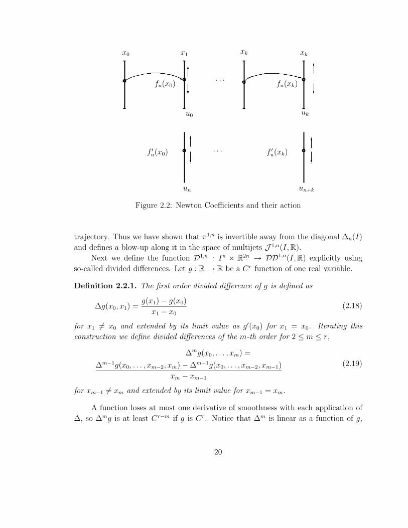
As Figure 2 illustrates, these considerations show that for any map f and any

desired trajectory of distinct points with any given derivatives along it, one can choose

Newton coefficients {uk}2n−1k=0 and explicitly construct a map fε = f + φε with such a

19

x0 x1 xkxk

fu(x0) fu(xk)

f ′u(x0) f ′

u(xk)

u0 uk

un un+k

· · ·

· · ·

Figure 2.2: Newton Coefficients and their action

trajectory. Thus we have shown that π1,n is invertible away from the diagonal ∆n(I)

and defines a blow-up along it in the space of multijets J 1,n(I, R).

Next we define the function D1,n : In × R2n → DD1,n(I, R) explicitly using

so-called divided differences. Let g : R → R be a Cr function of one real variable.

Definition 2.2.1. The first order divided difference of g is defined as

∆g(x0, x1) =g(x1) − g(x0)

x1 − x0

(2.18)

for x1 6= x0 and extended by its limit value as g′(x0) for x1 = x0. Iterating this

construction we define divided differences of the m-th order for 2 ≤ m ≤ r,

∆mg(x0, . . . , xm) =

∆m−1g(x0, . . . , xm−2, xm) − ∆m−1g(x0, . . . , xm−2, xm−1)

xm − xm−1

(2.19)

for xm−1 6= xm and extended by its limit value for xm−1 = xm.

A function loses at most one derivative of smoothness with each application of

∆, so ∆mg is at least Cr−m if g is Cr. Notice that ∆m is linear as a function of g,

20

and one can show that it is a symmetric function of x0, . . . , xm; in fact, by induction

it follows that

∆mg(x0, . . . , xm) =m∑

i=0

g(xi)∏

j 6=i(xi − xj)(2.20)

Another identity that is proved by induction will be more important for us, namely

∆m xk(x0, . . . , xm) = pk,m(x0, . . . , xm), (2.21)

where pk,m(x0, . . . , xm) is 0 for m > k and for m ≤ k is the sum of all degree k − m

monomials in x0, . . . , xm with unit coefficients,

pk,m(x0, . . . , xm) =∑

r0+···+rm=k−m

m∏

j=0

xrj

j . (2.22)

The divided differences are the right coefficients for the Newton interpolation

formula. For all C∞ functions g : R → R we have

g(x) =∆0g(x0) + ∆1g(x0, x1)(x − x0) + . . .

+ ∆n−1g(x0, . . . , xn−1)(x − x0) . . . (x − xn−2)

+ ∆ng(x0, . . . , xn−1, x)(x − x0) . . . (x − xn−1)

(2.23)

identically for all values of x, x0, . . . , xn−1. All terms of this representation are poly-

nomial in x except for the last one which we view as a remainder term. The sum of

the polynomial terms is the degree (n − 1) Newton interpolation polynomial for g at

{xk}n−1k=0 . To obtain a degree 2n − 1 interpolation polynomial for g and its derivative

at {xk}n−1k=0 , we simply use (2.23) with n replaced by 2n and the 2n-tuple of points

{xk(mod n)}2n−1k=0 .

Recall that D1,n was defined implicitly by (2.15). We have described how to

use divided differences to construct a degree 2n − 1 interpolating polynomial of the

form on the right-hand side of (2.15) for an arbitrary C∞ function g. Our interest

then is in the case g = φε, which as a degree 2n − 1 polynomial itself will have no

remainder term and coincide exactly with the interpolating polynomial. Thus D1,n is

given coordinate-by-coordinate by

um = ∆m

(2n−1∑

k=0

εkxk

)

(x0, . . . , xm (mod n))

= εm +2n−1∑

k=m+1

εkpk,m(x0, . . . , xm (mod n))

(2.24)

21

for m = 0, . . . , 2n − 1.

Equation (2.24) defines a transformation (u0, . . . , u2n−1) = L1Xn

(ε) on R2n, where

Xn = (x0, . . . , xn−1) ∈ In. We call L1Xn

the Newton map. This map is simply a

restriction of D1,n to its final 2n coordinates:

D1,n(Xn, ε) = (Xn,L1Xn

(ε)). (2.25)

Notice that for fixed Xn, the Newton map is linear and given by an upper triangular

matrix with units on the diagonal. Hence it is Lebesgue measure-preserving and

invertible, whether or not Xn lies on the diagonal ∆n(I).

Furthermore, the Newton map L1Xn

preserves the class of scaled Lebesgue product

measures introduced in (1.15). In general, a measure µ on R2n is a scaled Lebesgue

product measure if it is the product µ = µ0 × · · · × µ2n−1, where each µj is Lebesgue

measure on R scaled by a constant factor (which may depend on the coordinate j).

Since the L1Xn

only shears in coordinate directions, we have the following lemma.

Lemma 2.2.2. The Newton map L1Xn

given by (2.24) preserves all scaled Lebesgue

product measures.

This lemma will be used in Chapter 3. In the next section, we will introduce

the particular scaled Lebesgue product measure that the lemma will be applied to.

We call the basis of monomials

k∏

j=0

(x − xj(mod n)) for k = 0, . . . , 2n − 1 (2.26)

in the space of polynomials of degree 2n − 1 the Newton basis defined by the n-

tuple {xk}n−1k=0 . The Newton map and the Newton basis, and their analogues in di-

mension N , are useful tools for perturbing trajectories and estimating the measure

µn(C, δ, ρ,~r,M1+ρ) of “bad” parameter values ~ε ∈ HBN(r).

2.3 Estimates of the measure of “bad” parame-

ters and Fubini reduction to finite-dimensional

families

We return now to the the general case of C1+ρ diffeomorphisms on RN . In order

to bound µN~r {Bn(C, δ, ρ,~r, f)} we decompose the infinite-dimensional Hilbert Brick

22

HBN(~r) into the direct sum of a finite-dimensional brick of polynomials of degree

2n − 1 in N variables and its orthogonal complement.

Recall that ~r = ({rm}∞m=0) denotes the nonincreasing sequence {rm}m∈Z+ of sizes

of the Hilbert Brick. With the notation (1.11) and (1.12), define

HBN<k(~r) =

{{~εm}m<k : for every 0 ≤ m < k, ‖~εm‖m ≤ rm

}

=BN0 (r0) × · · · × BN

k−1(rk−1) ⊂ W0,N × W1,N × · · · × Wk−1,N ;

HBN≥k(~r) =

{{~εm}m≥k : for every m ≥ k, ‖~εm‖m ≤ rm

}

=BNk (rk) × BN

k+1(rk+1) × · · · ⊂ Wk,N × Wk+1,N × . . . ;

HBN(~r) =HBN<k(~r) ⊕ HBN

≥k(~r).

(2.27)

Each parameter ~ε ∈ HBN(~r) has a unique decomposition into

~ε =(~ε<k, ~ε≥k) ∈ HBN<k(~r) ⊕ HBN

≥k(~r),

φ~ε(x) =φ~ε<k(x) + φ~ε≥k

(x) =∑

|α|<k

~εαxα +∑

|α|≥k

~εαxα, (2.28)

where φ~ε<k(x) is a vector-polynomial of degree k−1 and φ~ε≥k

(x) is an analytic function

with all Taylor coefficients of order less than k being equal to zero. Recall the notation

(1.15), and decompose the measure µN~r on the brick HBN(~r) into the product

µN<k,~r = ×k−1

m=0 µNm,rm

, µN≥k,~r = ×∞

m=k µNm,rm

, µN~r = µN

<k,~r × µN≥k,~r. (2.29)

Thus, each component of the decomposition of the brick HBN<k(~r) (resp. HBN

≥k(~r)) is

supplied with the Lebesgue product probability measure µN<k,~r (resp. µN

≥k,~r). Denote

by

W<k,N = ×k−1m=0 Wm,N , W≥k,N = ×∞

m=k Wm,N (2.30)

the spaces to which the brick HBN<k(~r) and the Hilbert Brick HBN

≥k(~r) belong.

Consider the decomposition with k = 2n − 1. Suppose we can get an estimate

µN<2n,~r {Bn(C, δ, ρ,~r, f, ~ε≥2n)} ≤ µn(C, δ, ρ,M1+ρ) (2.31)

of the measure of the “bad” set

Bn(C, δ, ρ,~r, f, ~ε≥2n) = {~ε<2n ∈ HBN<2n(~r) :

f~ε ∈ IH(n − 1, C, δ, ρ) but f~ε /∈ IH(n,C, δ, ρ)}.(2.32)

in each slice HBN<2n(~r) × {~ε≥2n} ⊂ HBN(~r), uniformly over ~ε≥2n ∈ HBN

≥2n(~r). Then

by the Fubini/Tonelli Theorem and by the choice of the probability measure (2.29),

23

estimate (2.31) implies (2.3). Thus we reduce the problem of estimating measure of

the “bad” set (2.1) in the infinite-dimensional Hilbert Brick HBN(~r) to estimating

measure of the “bad” set (2.32) in the finite-dimensional brick HBN<2n(~r) of vector-

polynomials of degree 2n − 1. Now our main goal is to get an estimate for the

right-hand side of (2.31).

Fix a parameter value ~ε≥2n ∈ HBN≥2n(~r) and the corresponding parameter slice

HBN<2n(~r) × {~ε≥2n} in the Hilbert Brick HBN(~r). Let f = f(0,~ε≥2n) be the center of

this slice. In this slice we have the finite-parameter family

{f~ε<2n}~ε<2n∈HBN

<2n(~r) = {f(~ε<2n,~ε≥2n)}~ε<2n∈HBN<2n(~r) (2.33)

of perturbations by polynomials of degree 2n − 1. This is the family we consider

at the n-th stage of the induction. We redenote the “bad” set of parameter values

Bn(C, δ, ρ,~r, f, ~ε≥2n) by Bn(C, δ, ρ,~r, f).

2.4 Simple trajectories and the Inductive Hypoth-

esis

Based on the discussion in Section 2.1, we make the following definition.

Definition 2.4.1. A trajectory x0, . . . , xn−1 of length n of a diffeomorphism f ∈Diffr(BN), where xk = fk(x0), is called (n, γ)-simple if

n−2∏

k=0

|xn−1 − xk| ≥ γ1/4N . (2.34)

A point x0 is called (n, γ)-simple if its trajectory {xk = fk(x0)}n−1k=0 of length n is

(n, γ)-simple. Otherwise a point (resp. a trajectory) is called non-(n, γ)-simple.

If a trajectory is simple, then perturbation of this trajectory by Newton Interpo-

lation Polynomials is effective as the Closing Lemma and Perturbation of hyperbolic-

ity examples of Section 2.1 show. To evaluate the product of distances it is important

to choose a “good” starting point x0 of an almost periodic trajectory {xk}k in order

to have the largest possible value of the product in (2.34); for some starting points

the product of distances may be artificially small.

Consider the following example of a homoclinic intersection: Let f : B2 → B2

be a diffeomorphism with a hyperbolic saddle point at the origin f(0) = 0. Suppose

that the stable manifold W s(0) and the unstable manifold W u(0) intersect at some

24

point q ∈ W s(0) ∩ W u(0). Then for a sufficiently large n there is a periodic point x

of period n in a neighborhood of q going once nearby 0. It is clear that the trajectory

{fk(x)}nk=1 spends a lot of time in a neighborhood of the origin. Choose two starting

points x′0 = fk′

(x) and x′′0 = fk′′

(x) for the product (2.34). If x′0 is not in an exp(−εn)-

neighborhood of the origin for some ε > 0, but x′′0 is, then it might happen that

∏n−2k=0 |fn−1(x′

0)−fk(x′0)| ∼ exp(−δn) and

∏n−2k=0 |fn−1(x′′

0)−fk(x′′0)| ∼ exp(−δ′n2) for

some δ, δ′ > 0. Indeed, if we pick out of {fk(x)}nk=1 only the n/2 closest to the origin,

then a simple calculation shows that all of them are in an exp(−εn)-neighborhood of

the origin, where ε is some positive number depending on the eigenvalues of df(0). So

the first product might be significantly larger than the second one. This is because the

trajectory {fk(x′′0)}n−1

k=0 has many points in a neighborhood of the origin and all of the

corresponding terms in the product are small. This shows that sometimes the product

of distances along a trajectory (2.34) might be small not because the trajectory is too

recurrent, but because we choose a “bad” starting point. This motivates the following

definition.

Definition 2.4.2. A point x is called essentially (n, γ)-simple if for some nonnegative

j < n, the point f j(x) is (n, γ)-simple. Otherwise a point is called essentially non-

(n, γ)-simple.

Let us return to the strategy of the proof of Theorem 1.3.7. At the n-th stage

of the induction over the period we consider the family of polynomial perturbations

{f~ε<2n}~ε<2n∈HBN

<2n(~r) of the form (2.33) of the diffeomorphism f ∈ Diff1+ρ(BN) by

polynomials of degree 2n− 1. Consider among them only diffeomorphisms f~ε<2nthat

satisfies Inductive Hypothesis of order n − 1 with constants (C, δ, ρ), i.e. f~ε<2n∈

IH(n − 1, C, δ, ρ) as we proposed earlier. To simplify notations we redenote the set

Bn(C, δ, ρ,~r, f, ~ε≥2n) by Bn(C, δ, ρ,~r, f) with f = f~ε≥2n. Our main goal is to estimate

measure of “bad” parameter values Bn(C, δ, ρ,~r, f), given by (2.32), for which the

corresponding diffeomorphism has an (n, γ1/ρn (C, δ))-periodic, but not (n, γn(C, δ))-

hyperbolic, point x ∈ BN .

We split the set of all possible almost periodic points of period n into two classes:

essentially (n, γ1/Nn (C, δ))-simple and essentially non-(n, γ

1/Nn (C, δ))-simple. Decom-

pose the set of “bad” parameters Bn(C, δ, ρ,~r, f) into two sets of “bad” parameters

with simple and nonsimple almost periodic points that are not sufficiently hyperbolic:

Bsimn (C, δ, ρ,~r, f) = {~ε ∈ HBN(~r) : f~ε<2n

∈ IH(n − 1, C, δ, ρ),

f~ε<2nhas an (n, γ1/ρ

n (C, δ))-periodic, essentially

(n, γ1/Nn (C, δ))-simple, but not (n, γn(C, δ))-hyperbolic point x}

(2.35)

25

and

Bnonn (C, δ, ρ,~r, f) = {~ε ∈ HBN(~r) : f~ε<2n

∈ IH(n − 1, C, δ, ρ),

f~ε<2nhas an (n, γ1/ρ

n (C, δ))-periodic, essentially

non-(n, γ1/Nn (C, δ))-simple, but not (n, γn(C, δ))-hyperbolic point x}

(2.36)

It is clear that we have

Bn(C, δ, ρ,~r, f) = Bsimn (C, δ, ρ,~r, f) ∪ Bnon

n (C, δ, ρ,~r, f). (2.37)

We shall estimate the measures of the sets of simple orbits Bsimn (C, δ, ρ,~r, f) and

nonsimple orbits Bnonn (C, δ, ρ,~r, f) separately, but using very similar methods.

Let f~ε<2n∈ IH(n − 1, C, δ, ρ) be a diffeomorphism that satisfies the Inductive

Hypothesis of order n − 1 with constants (C, δ, ρ). It turns out that if f~ε<2nhas

an (n, γ1/ρn (C, δ))-periodic and essentially non-(n, γ

1/Nn (C, δ))-simple point x0, then

the trajectory of x0 has a close return fk~ε<2n

(x0) = xk for k < n such that distance

|x0 − xk| is much smaller of all the previous |x0 − xj|, 1 ≤ j < k. Let us formulate

more precisely what we mean here by “much smaller”.

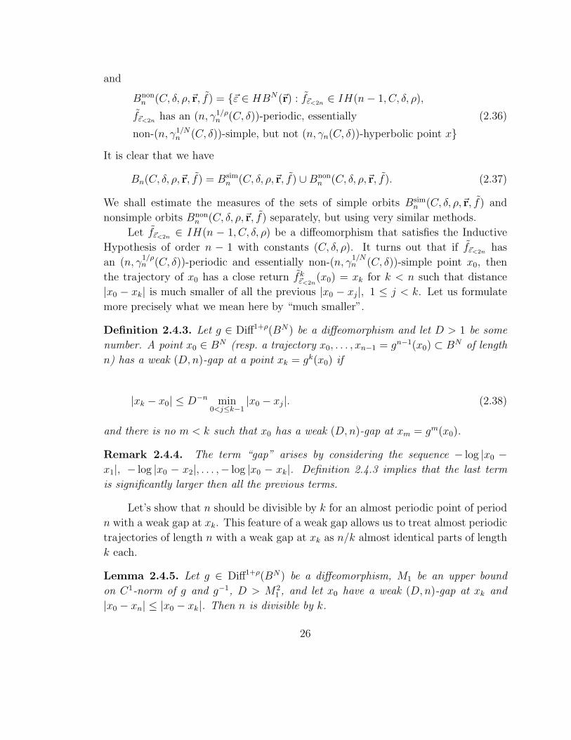
Definition 2.4.3. Let g ∈ Diff1+ρ(BN) be a diffeomorphism and let D > 1 be some

number. A point x0 ∈ BN (resp. a trajectory x0, . . . , xn−1 = gn−1(x0) ⊂ BN of length

n) has a weak (D,n)-gap at a point xk = gk(x0) if

|xk − x0| ≤ D−n min0<j≤k−1

|x0 − xj|. (2.38)

and there is no m < k such that x0 has a weak (D,n)-gap at xm = gm(x0).

Remark 2.4.4. The term “gap” arises by considering the sequence − log |x0 −x1|, − log |x0 − x2|, . . . ,− log |x0 − xk|. Definition 2.4.3 implies that the last term

is significantly larger then all the previous terms.

Let’s show that n should be divisible by k for an almost periodic point of period

n with a weak gap at xk. This feature of a weak gap allows us to treat almost periodic

trajectories of length n with a weak gap at xk as n/k almost identical parts of length

k each.

Lemma 2.4.5. Let g ∈ Diff1+ρ(BN) be a diffeomorphism, M1 be an upper bound

on C1-norm of g and g−1, D > M21 , and let x0 have a weak (D,n)-gap at xk and

|x0 − xn| ≤ |x0 − xk|. Then n is divisible by k.

26

Sketch of Proof: Denote by gcd(k, n) the greatest common divisor of k and n.

Then using the bound on C1-norm of g and g−1 for any x, y ∈ BN we have

M−11 |g−1(x) − g−1(y)| ≤ |x − y| ≤ M1 |g(x) − g(y)| (2.39)

Using the Euclidean division algorithm developed in Part II of this paper, one can

show that

|x0 − xgcd(k,n)| ≤ M2n1 D−n min

0<j≤k−1|x0 − xj|. (2.40)

Since D > M21 , we cannot have gcd(k, n) < k, so n must be divisible by k. Q.E.D.

In Part II of this paper we prove the following result.

Theorem 2.4.6. Let g ∈ Diff1+ρ(BN) be a diffeomorphism for some ρ > 0 and

satisfy the Inductive Hypothesis of order n−1 with constants (C, δ, ρ), i.e. g ∈ IH(n−1, C, δ, ρ) and let M1+ρ = max{‖g−1‖C1 , ‖g‖C1+ρ , 21/ρ}, C > 100ρ−1δ−1 log M1+ρ, and

D = max{M30/ρ1+ρ , exp (C/100)}. Suppose the diffeomorphism g has an (n, γ

1/ρn (C, δ))-

periodic and essentially non-(n, γ1/Nn (C, δ))-simple point x0 ∈ BN . Then either x0

is (n, γn(C, δ))-hyperbolic or x0 has a weak (D,n)-gap at xk = gk(x0) for some k

dividing n and xj is (k, γ1/Nn (C, δ))-simple for some j < n.

Remark 2.4.7. As a matter of fact we need a sharper result, but Theorem 2.4.6 is a

nice starting point.

Theorem 2.4.6 implies that the set of “bad” parameters with an essentially non-

simple trajectory can be decomposed into the following finite union: Define the set

of parameters with an almost periodic point of period n with a weak gap at the k-th

point of its trajectory.

Bwgap(k)n (C, δ, ρ,~r, f ; D) = {~ε ∈ HBN(~r) : f~ε ∈ IH(n − 1, C, δ, ρ),

f~ε has an (n, γ1/ρn (C, δ))-periodic, but not

(n, γn(C, δ))-hyperbolic point x0 with a weak (D,n)-gap at xk = fk~ε (x)}

(2.41)

Then for D = max{M30/ρ1+ρ , exp(C/100)}, Theorem 2.4.6 gives

Bnonn (C, δ, ρ,~r, f) ⊆

(

∪k|nBwgap(k)n (C, δ, ρ,~r, f ; D)

)

. (2.42)

Combining inclusions (2.35) and (2.42), we have

Bn(C, δ, ρ,~r, f) ⊆Bsim

n (C, δ, ρ,~r, f) ∪(

∪k|nBwgap(k)n (C, δ, ρ,~r, f ; D)

)

.(2.43)

27

Thus we need to get estimates on the measures of bad parameters associated

with essentially simple trajectories Bsimn (C, δ, ρ,~r, f) and trajectories with a weak gap

Bwgap(k)n (C, δ, ρ,~r, f ; D), where k divides n. In Chapter 3, we describe the Discretiza-

tion method for the 1-dimensional model problem. This method will allow us to

estimate the measure of parameters Bsimn (C, δ, ρ,~r, f) associated with simple almost

periodic points. At the end of Chapter 3, we show how using the Discretization

method one can estimate the measure of parameters Bwgap(k)n (C, δ, ρ,~r, f ; D) associ-

ated with almost periodic trajectories with a weak gap. Loosely speaking, it is because

those trajectories have simple parts of length k (see the end of Theorem 2.4.6), and

hyperbolicity of simple part of length k enforces hyperbolicity of the trajectories of

length n.

28

Chapter 3

A Model Problem: C2-smooth

Maps of the Interval I = [−1, 1]

In Section 2.4 we concluded that the key to the proof of Theorem 1.3.7 (which implies

the Main Theorem) is to get an estimate of the measure of “bad” parameters. Recall

that the set of “bad” parameters (2.32) consists of those parameters ~ε ∈ HBN(~r) for

which the corresponding diffeomorphism f~ε : BN → BN has an almost periodic point

x of period n that is not sufficiently hyperbolic. In this chapter we present a detailed

discussion of C2-smooth 1-dimensional noninvertible maps (N = 1 and ρ = 1) with

a Hilbert Brick of a “nice” size. This 1-dimensional model gives a useful insight

into the general approach of estimating the measure of “bad” parameters for the N -

dimensional C1+ρ-smooth diffeomorphisms and allows us to avoid several technical

complications that will arise in Part II of this paper [K5]. These complications are

outlined in the next chapter.

3.1 Setting up of the model

Let C2(I, I) be the space of C2-smooth maps of the interval I = [−1, 1] into its

interior. Consider a C2-smooth map of the interval f ∈ C2(I, I) and the family of

perturbations of f by analytic functions represented as their power series

fε(x) = f(x) +∞∑

k=0

εkxk. (3.1)

Fix a positive τ > 0. Define a range of parameters of this family in the form of

29

a Hilbert Brick

HBst(τ) ={

{εm}∞m=0 : ∀ m ≥ 0, |εm| <τ

m!

}

. (3.2)

We call HBst(τ) a Hilbert Brick of standard thickness with width τ . If we choose τ

small enough, then the whole family {fε}ε∈HBst(τ) ⊂ C2(I, I) consists of C2-smooth

maps of the interval I.

Define the Lebesgue product probability measure, denoted by µstτ , on the Hilbert

Brick of parameters HBst(τ) by normalizing the 1-dimensional Lebesgue measure

along each component to the 1-dimensional Lebesgue probability measure

µstm,τ =

(m!

2τ

)

Leb1, µst<k,τ = ×k−1

m=0 µstm,τ µst

τ = ×∞m=0 µst

m,τ . (3.3)

The main result of this Chapter is the following 1-dimensional analogue of Theorem

1.3.7.

Theorem 3.1.1. Let f ∈ C2(I, I) be a C2-smooth map of the interval I into its inte-

rior and let τ > 0 be so small that the family of analytic perturbations {fε}ε∈HBst(τ) ⊂C2(I, I) consists of C2-smooth maps of the interval I. Then for any δ > 0 and µst

τ -

a.e. ε ∈ HBst(τ) there exists C = C(ε, δ) > 0 such that the number of periodic points

Pn(fε) of fε of period n and their minimal hyperbolicity γn(fε), defined in (1.7), for

all n ∈ Z+ satisfy

γn(fε) > exp(−Cn1+δ), Pn(fε) < exp(Cn1+δ). (3.4)

The strategy for the proof of this Theorem is the same as the strategy of the proof

of Theorem 1.3.7 described in Chapter 2. Denote the supremum C2 and C1-norms of

the family (3.1)

M1 = supε∈HBst(τ)

{‖fε‖C1}, M2 = supε∈HBst(τ)

{‖fε‖C2 ,M1, 2} (3.5)

By analogy with the direct decomposition of the Hilbert Brick in the N -dimen-

sional case (2.27), for each positive integer k ∈ Z+ define the direct decomposition of

the Hilbert Brick of standard thickness HBst(τ)

HBst<k(τ) =

{

{εm}k−1m=0 : ∀ 0 ≤ m < k, |εm| <

τ

m!

}

.

HBst≥k(τ) =

{

{εm}∞m=k : ∀ m ≥ k, |εm| <τ

m!

}

.(3.6)

30

We call HBst<k(τ) a (k-dimensional) Brick of standard thickness with width τ . The

product measure µstτ on the whole Hilbert Brick HBst(τ) induces the measure of

product of Lebesgue probability µst<k,τ on the k-dimensional Brick HBst

<k(τ).

Fix n ∈ Z+ and consider the n-th stage of the induction over the period (see the

beginning of Chapter 2). Let

f(x) = f(x) +∞∑

k=2n

εkxk (3.7)

for some {εk}∞k=2n ∈ HBst≥2n(τ), and consider the 2n-parameter family of pertur-

bations by polynomials of degree 2n − 1 with coefficients in the brick of standard

thickness HBst<2n(τ),

fε(x) = f(x) +2n−1∑

k=0

εkxk, ε = (ε0, . . . , ε2n−1) ∈ HBst

<2n(τ). (3.8)

The bounds M1 and M2 from (3.5) apply to this subfamily of (3.1).

Using the Fubini reduction to finite-dimensional families from Section 2.3 right

after (2.31), for the proof of Theorem 3.1.1 it is sufficient to estimate the measure of

“bad” parameters in each such a family.

To fit the notations of our model we choose a sufficiently small positive γn and

we introduce sets of all “bad” parameters (compare with (2.32))

Bn,τ (C, δ, f , γn) = {ε ∈ HBst<2n(τ) : fε ∈ IH(n − 1, C, δ, 1),

fε has an (n, γn)-periodic, but not (n, γn)-hyperbolic point x0},(3.9)

and define the sets Bsimn,τ (C, δ, f , γn) and Bnon

n,τ (C, δ, f , γn) of “bad” parameters with

essentially simple (respectively nonsimple) trajectories as in (2.35) and (2.36):

Bsimn (C, δ, f , γn) = {~ε ∈ HBst

<2n(τ) : fε ∈ IH(n − 1, C, δ, 1),

fε has an (n, γn)-periodic, essentially

(n, γn)-simple, but not (n, γn)-hyperbolic point x0},(3.10)

and

Bnonn (C, δ, f , γn) = {~ε ∈ HBst

<2n(τ) : fε ∈ IH(n − 1, C, δ, 1),

fε has an (n, γn)-periodic, essentially

non-(n, γn)-simple, but not (n, γn)-hyperbolic point x0}.(3.11)

31

For sufficiently small γn, e.g., γn ≤ γn(C, δ), similarly to (2.37) we have the

following decomposition

Bn,τ (C, δ, f , γn) = Bsimn,τ (C, δ, f , γn) ∪ Bnon

n,τ (C, δ, f , γn). (3.12)

The main result of the next three sections is the following estimate.

Proposition 3.1.2. Let {fε}ε∈HBst<2n(τ) be the family of polynomial perturbations (3.8)

with bound M2 on the C2-norm. Then with the notation above, for any C > 2, δ > 0,

and τ > 0 and a sufficiently small positive γn, e.g., γn ≤ γn(C, δ), the following esti-

mate on the measure of parameters associated with maps fε with an (n, γn)-periodic,

essentially (n, γn)-simple, but not (n, γn)-hyperbolic, point holds

µst<2n,τ

{Bsim

n,τ (C, δ, f , γn)}≤ 62nM6n+1

2

(n − 1)!

τ

(2n − 1)!

τγ1/4

n . (3.13)

It is clear that for any C > 0 and δ > 0, if γn = exp(−Cn1+δ), then the

right-hand side of (3.13) tends to 0 as n → ∞ superexponentially fast in n. An

estimate on the measure of essentially nonsimple trajectories µst<2n,τ

{Bnon

n (C, δ, f , γn)}

is obtained in Section 3.5, Proposition 3.5.1. Application of these two Propositions

and arguments (2.3–2.4) will prove Theorem 3.1.1. The method of obtaining an

estimate for µst<2n,τ

{Bnon

n,τ (C, δ, f , γn)}

is similar to the one we shall develop now to

prove (3.13).

3.2 Decomposition into pseudotrajectories

In this section, we decompose the set of “bad” parameters Bsimn,τ (C, δ, f , γn) for which

there exists a simple, almost periodic, but not sufficiently hyperbolic trajectory into a

finite union of sets of “bad” parameters. Each set will be associated with a particular

simple, almost periodic, but not sufficiently hyperbolic pseudotrajectory. In the next

section we will estimate the measure of “bad” parameters associated with a particular

trajectory, and in the subsequent section we will extend this estimate to the set of

“bad” parameters associated with all possible simple trajectories, obtaining estimate

(3.13).

Fix a sufficiently small γn > 0 and γn = γnM−2n2 . Consider the 2γn-grid in the

interval I

Iγn= {x ∈ I : ∃k ∈ Z such that x = (2k + 1)γn} ⊂ I (3.14)

32

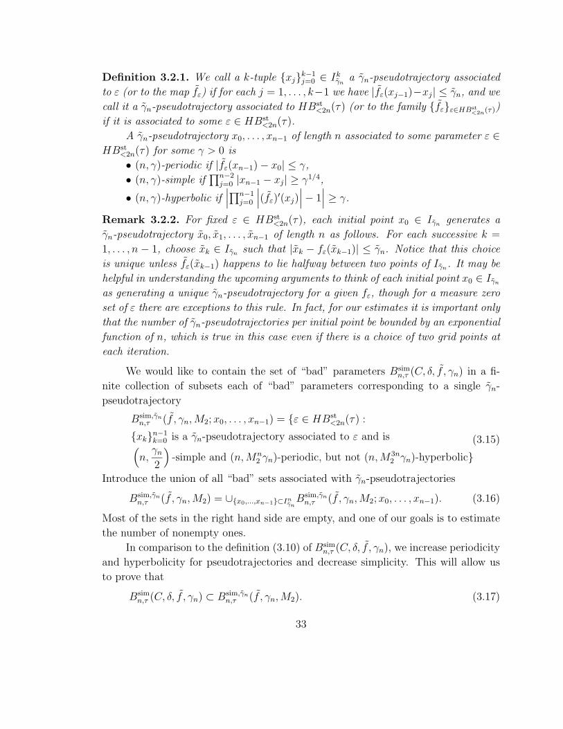
Definition 3.2.1. We call a k-tuple {xj}k−1j=0 ∈ Ik

γna γn-pseudotrajectory associated

to ε (or to the map fε) if for each j = 1, . . . , k−1 we have |fε(xj−1)−xj| ≤ γn, and we

call it a γn-pseudotrajectory associated to HBst<2n(τ) (or to the family {fε}ε∈HBst

<2n(τ))

if it is associated to some ε ∈ HBst<2n(τ).

A γn-pseudotrajectory x0, . . . , xn−1 of length n associated to some parameter ε ∈HBst

<2n(τ) for some γ > 0 is

• (n, γ)-periodic if |fε(xn−1) − x0| ≤ γ,

• (n, γ)-simple if∏n−2

j=0 |xn−1 − xj| ≥ γ1/4,

• (n, γ)-hyperbolic if∣∣∣∏n−1

j=0

∣∣∣(fε)

′(xj)∣∣∣ − 1

∣∣∣ ≥ γ.

Remark 3.2.2. For fixed ε ∈ HBst<2n(τ), each initial point x0 ∈ Iγn

generates a

γn-pseudotrajectory x0, x1, . . . , xn−1 of length n as follows. For each successive k =

1, . . . , n − 1, choose xk ∈ Iγnsuch that |xk − fε(xk−1)| ≤ γn. Notice that this choice

is unique unless fε(xk−1) happens to lie halfway between two points of Iγn. It may be

helpful in understanding the upcoming arguments to think of each initial point x0 ∈ Iγn

as generating a unique γn-pseudotrajectory for a given fε, though for a measure zero

set of ε there are exceptions to this rule. In fact, for our estimates it is important only

that the number of γn-pseudotrajectories per initial point be bounded by an exponential

function of n, which is true in this case even if there is a choice of two grid points at

each iteration.

We would like to contain the set of “bad” parameters Bsimn,τ (C, δ, f , γn) in a fi-

nite collection of subsets each of “bad” parameters corresponding to a single γn-

pseudotrajectory

Bsim,γnn,τ (f , γn,M2; x0, . . . , xn−1) = {ε ∈ HBst

<2n(τ) :

{xk}n−1k=0 is a γn-pseudotrajectory associated to ε and is

(

n,γn

2

)

-simple and (n,Mn2 γn)-periodic, but not (n,M3n

2 γn)-hyperbolic}(3.15)

Introduce the union of all “bad” sets associated with γn-pseudotrajectories

Bsim,γnn,τ (f , γn,M2) = ∪{x0,...,xn−1}⊂In

γnBsim,γn

n,τ (f , γn,M2; x0, . . . , xn−1). (3.16)

Most of the sets in the right hand side are empty, and one of our goals is to estimate

the number of nonempty ones.

In comparison to the definition (3.10) of Bsimn,τ (C, δ, f , γn), we increase periodicity

and hyperbolicity for pseudotrajectories and decrease simplicity. This will allow us

to prove that

Bsimn,τ (C, δ, f , γn) ⊂ Bsim,γn

n,τ (f , γn,M2). (3.17)

33

Intuitively this is true because each trajectory of length n can be approximated by a

pseudotrajectory of length n which has almost the same periodicity, simplicity, and

hyperbolicity as the original one. We will make this argument precise at the end of

Section 3.4.

Remark 3.2.3. Unlike Bsimn,τ (C, δ, f , γn), we do not assume in the definition (3.15) of

Bsim,γnn,τ (f , γn,M2) that fε ∈ IH(n−1, C, δ, 1). This is because we only need the Induc-

tive Hypothesis to estimate the measure of “bad” parameters in the case of nonsimple

trajectories.

Our goal is then to estimate the measure µst<2n,τ

{Bsim,γn

n,τ (f , γn,M2)}

in order

to prove Proposition 3.1.2. Loosely speaking, this measure will be estimated in two

steps:

Step 1. Estimate the number of different γn-pseudotrajectories #n(γn, τ) associated

to HBst<2n(τ);

Step 2. Estimate the measure

µst<2n,τ

{Bsim,γn

n,τ (f , γn,M2; x0, . . . , xn−1)}≤ µn(M2, γn, γn, τ) (3.18)

uniformly for an (n, γn)-simple γn-pseudotrajectory {x0, . . . , xn−1} ∈ Inγn

.

Then the product of two numbers #n(γn, τ) and µn(M2, γn, γn, τ) that are obtained

in Steps 1 and 2 gives the required estimate (3.13).

Actually the procedure of estimating µst<2n,τ

{Bsim,γn

n,τ (f , γn,M2)}

is a little more

complicated. Based on the definition (3.15) of the set Bsim,γnn,τ (f , γn,M2; x0, . . . , xn−1)

of parameters ε for which the diffeomorphism fε has a prescribed γn-pseudotrajectory

{x0, . . . , xn−1} ∈ Inγn

that is almost periodic and not sufficiently hyperbolic, define a

set of parameters ε for which only a part of the γn-pseudotrajectory {x0, . . . , xm−1} ∈Imγn

is prescribed for fε:

Bsim,γnn,τ (f , γn,M2; x0, . . . , xm−1) = {ε ∈ HBst

<2n(τ) : there exist

xm, . . . , xn−1 ∈ Iγnsuch that {xj}n−1

j=0 is a γn-pseudotrajectory

associated to ε, and ε ∈ Bsim,γnn,τ (f , γn,M2; x0, . . . , xn−1)}.

(3.19)

For each m = 1, 2, . . . , n − 1 it is clear that

Bsim,γnn,τ (f , γn,M2; x0, . . . , xm−1) = ∪xm∈Iγn

Bsim,γnn,τ (f , γn,M2; x0, . . . , xm). (3.20)

34

Inductive application of this formula to the definition (3.16) yields

Bsim,γnn,τ (f , γn,M2) = ∪x0∈Iγn

Bsim,γnn,τ (f , γn,M2; x0). (3.21)

The estimate of Step 1 then breaks down as follows:

#n(γn, τ) ≈ # of initial

points of Iγn

× # of γn-pseudotrajectories

per initial point(3.22)

And up to an exponential function of n, the estimate of Step 2 breaks down like:

µn(M2, γn, γn, τ) ≈

Measure of

periodicity× Measure of

hyperbolicity

# of γn-pseudotrajectories

per initial point

(3.23)

(Roughly speaking, the terms in the numerator represent respectively the measure of

parameters for which a given initial point will be (n, γn)-periodic and the measure

of parameters for which a given n-tuple is (n, γn)-hyperbolic; they correspond to

estimates (3.30) and (3.33) in the next section.) Thus after cancellation, the estimate

of the measure of “bad” set Bsimn,τ (C, δ, f , γn) associated to simple, almost periodic,

not sufficiently hyperbolic trajectories becomes:

Measure of bad

parameters≤

# of initial

points of Iγn

× Measure of

periodicity× Measure of

hyperbolicity

(3.24)

The first term on the right hand side of (3.24) is of order γ−1n (up to an expo-

nential function in n). In Section 3.3, we will show that the second term is at most

of order n!γ3/4n , and the third term is at most of order (2n)!γ

1/2n , so that the product

on the right-hand side of (3.24) is of order at most n!(2n)!γ1/4n (up to an exponential

function in n) and is superexponentially small in n. These bounds use the change of

parameter coordinates by Newton interpolation polynomials that was introduced in

Section 2.2, and they do not depend on whether the parameters are associated with

the brick HBst<2n(τ), except in that we use the bound M2 on the C2 norm of the maps

involved.

35

In Section 3.4, we complete the proof of Proposition 3.1.2 by bounding the

total measure of “bad” parameters for all pseudotrajectories associated to HBst<2n(τ).

Since we use the Fubini theorem in the Newton coordinates u0, . . . , u2n−1, we need

to know the maximum range of each of these parameters in the image of HBst<2n(τ)

under this coordinate change. In the “Distortion Lemma”, we show that the image

of HBst<2n(τ) is contained in a brick 3 times as large in each direction. Then, in the

“Collection Lemma”, we show in effect that the cancellation in going from (3.22)

and (3.23) to (3.24) is valid. In fact, the number of γn-pseudotrajectories for a given

initial point may depend significantly on the initial point, and we do not bound it

explicitly. Rather, we show that in the decomposition (3.21), the measure of each

term Bsim,γnn,τ (f , γn,M2; x0) is bounded (up to a factor exponential in n) by the product

of the “measure of periodicity” and “measure of hyperbolicity” derived in Section 3.3,

thus yielding a final estimate of the form (3.24).

3.3 Application of Newton interpolation polyno-

mials to estimate the measure of “bad” pa-

rameters for a single trajectory

In this section we fix an n-tuple of points {xj}n−1j=0 ∈ In, denoted by Xn, and estimate

the measure of “bad” parameters Bsim,γnn,τ (f , γn,M2; x0, . . . , xn−1)

}associated with this

particular trajectory. Recall that γn = M−2n2 γn.

Problem 3.3.1. Estimate the measure of ε ∈ HBst<2n(τ) for which the n-tuple {xj}n−1

j=0

is

A) a γn-pseudotrajectory, i.e., |fε(xj) − xj+1| ≤ γn for j = 0, . . . , n − 2;

B) (n, γn)-periodic, i.e., |fε(xn−1) − x0| ≤ γn; and

C) not (n, γn)-hyperbolic, i.e.,

∣∣∣∣∣

n−1∏

j=0

|(fε)′(xj)| − 1

∣∣∣∣∣≤ γn.

(3.25)

Recall the definitions and notation of Sections 2.2 and 2.3. In particular, W<2n,1

is the space of polynomials of degree 2n − 1 with the standard basis {xm}2n−1m=0 . The

measure µst<2n,τ defined on the brick HBst

<2n(τ) ∈ W<2n,1 by (3.3) extends naturally

to W<2n,1 using the same formulas. Denote by W u,Xn

<2n,1 the same space of polynomials

of degree 2n − 1, but with the Newton basis (2.26). Lemma 2.2.2 implies that the

Newton Map L1Xn

: W<2n,1 → W u,Xn

<2n,1 defined by (2.24) preserves the measure µst<2n,τ .

36

In other words, the definition (3.3) produces the same measure whether the standard

basis or Newton basis is used.

Now we will estimate the measure of “bad” parameters for a particular trajectory

using the Newton basis, without regard (except in the final hyperbolicity estimate)

to whether the parameters u = (u0, u1, . . . , u2n−1) lie in the image L1Xn

(HBst<2n(τ)) of

the brick we are concerned with. For a fixed n-tuple of points Xn = {xj}n−1j=0 , consider

the Newton family of polynomial perturbations

fu,Xn(x) = f(x) +

2n−1∑

m=0

um

m−1∏

j=0

(x − xj (mod n)). (3.26)

Notice that in (2.17) and Figure 2.2, the image fu,Xn(x0) of x0 is independent of

uk for all k > 0. Therefore, the position of fu,Xn(x0) depends only on u0. Recall that

µstm,τ is 1-dimensional Lebesgue measure scaled by m!/(2τ). This gives

µst0,τ

{

u0 :∣∣∣fu,Xn

(x0) − x1

∣∣∣ =

∣∣∣f(x0) + u0 − x1

∣∣∣ ≤ γn

}

≤ 0!

2τ2γn =

0! γn

τ(3.27)

Fix u0. Similarly, the position of fu(x1) depends only on u1 (see (2.17) and Fig. 2.2).

Thus, we have

µst1,τ

{u1 :

∣∣∣fu,Xn

(x1) − x2

∣∣∣ =

∣∣∣f(x1) + u0 + u1(x1 − x0) − x2

∣∣∣ ≤ γn

}≤ 1! γn

τ |x1 − x0|(3.28)

Inductively for k = 2, . . . , n− 1, fix u0, . . . , uk−1. Then the position of fu,Xn(xk)

depends only on uk. Moreover, for k = 2, . . . , n − 2 we have

µstk,τ

{

uk :∣∣∣fu,Xn

(xk) − xk+1

∣∣∣ =

∣∣∣∣∣f(xk) +

k∑

m=0

um

m−1∏

j=0

(xk − xj) − xk+1

∣∣∣∣∣≤ γn

}

≤ k!

τ

γn∏k−1

j=0 |xk − xj|,

(3.29)

and for k = n − 1 we have

µstn−1,τ

{un−1 :

∣∣∣fu,Xn

(xn−1) − x0

∣∣∣ ≤ γn

}≤ (n − 1)!

τ

γn∏n−2

j=0 |xn−1 − xj|. (3.30)

In particular, the parameter un−1 is responsible for (n, γn)-periodicity of the n-tuple

Xn. Formula (3.30) estimates the “measure of periodicity” discussed in the previous

section.

37

Choose u0, . . . , un−1 so that the n-tuple Xn is a γn-pseudotrajectory and is

(n, γn)-periodic. Notice that parameters un, un+1, . . . , u2n−1 do not change the γn-

pseudotrajectory {xk}n−1k=0 . Fix now parameters u0, . . . , u2n−2 and vary only u2n−1.

Then for any C1-smooth map g : I → I, consider the 1-parameter family

gu2n−1(x) = g(x) + (x − xn−1)n−2∏

j=0

(x − xj)2 (3.31)

Since the corresponding monomial (x− xn−1)∏n−2

j=0 (x− xj)2 has zeroes of the second

order at all points xk, except the last one xn−1, we have

n−1∏

j=0

(gu2n−1)′(xj) =

(

g′(xn−1) + u2n−1

n−2∏

j=0

|xn−1 − xj|2)

n−2∏

j=0

g′(xj). (3.32)

To get the final estimate, we use the fact that we are interested only in maps

from the family {fε}ε∈HBst<2n(τ). Therefore, we have |f ′

u,Xn(xn−1)| ≤ M1 ≤ M2. For

condition (C) of (3.25) to hold,∣∣∣∏n−1

j=0 f ′u,Xn

(xj)∣∣∣ must lie in [1 − γn, 1 + γn]. If this

occurs for any u2n−1 = ε2n−1 ∈ HBst2n(τ), then

∣∣∣∏n−2

j=0 f ′u,Xn

(xj)∣∣∣ ≥ (1 − γn)/M2 for

all u2n−1, because this product does not depend on u2n−1. Using (3.32) and the fact

that 1 − γn ≥ 1/2, we get

µst2n−1,τ

{

u2n−1 :

∣∣∣∣∣

n−1∏

j=0

|(fu,Xn)′(xj)| − 1

∣∣∣∣∣≤ γn

}

≤

2M2(2n − 1)!

2τ

4γn∏n−2

j=0 |xn−1 − xj|2= 4M2

(2n − 1)!

τ

γn∏n−2

j=0 |xn−1 − xj|2.

(3.33)

This formula estimates the “measure of hyperbolicity” discussed in the previous sec-

tion.

By Lemma 2.2.2, we can combine all these estimates and get

µst<n,τ × µst

2n−1,τ{(u0, . . . , un−1, u2n−1) ∈ W u,Xn

<n,1 × W u,Xn

2n−1,1 :

fu,Xnsatisfies conditions (3.25) and ‖fu,Xn

‖C2 ≤ M2} ≤

4M2(n − 1)! γn

τ∏n−2

j=0 |xn−1 − xj|(2n − 1)! γn

τ∏n−2

j=0 |xn−1 − xj|2n−2∏

m=0

m! γn

τ∏m−1

j=0 |xm − xj|,

(3.34)

where the spaces W u,Xn

<n,1 and W u,Xn

2n−1,1 are discussed in the beginning of this section.

This estimate corresponds loosely to (3.23) in the previous section. The final term

38

is an upper bound on measure of parameters for which Xn is a γn-pseudotrajectory

for fu,Xn. Roughly speaking, since almost every initial point x0 has exactly one

γn-pseudotrajectory Xn ∈ Inγn

for each set of parameters, and the total measure of

parameters in HBst<2n(τ) is 1, the sum over all γn-pseudotrajectories Xn associated

to x0 and HBst<2n(τ) of the parameter measure associated with Xn should be 1. Thus

the final term on the right-hand side of (3.34) also represents an upper bound on

the inverse of the number of γn-pseudotrajectories per initial point, which appears in

(3.23). However, we need the upper bound to be sharp in order to cancel this term

with that in (3.22), and the heuristic explanation of this paragraph is complicated by

the fact that the parameterization we are using depends on the γn-pseudotrajectory

Xn. These challenges will be resolved in the Collection Lemma of the next section.

3.4 The Distortion and Collection Lemmas

In this section we formulate the Distortion Lemma for the Newton map L1Xn

, and

complete the estimate of the measure of all “bad” parameters with a simple, almost

periodic, but not sufficiently hyperbolic trajectory (3.13) by collecting all possible

“bad” pseudotrajectories (see the Collection Lemma below).

Consider an ordered n-tuple of points Xn = {xj}n−1j=0 ∈ In and the Newton

map L1Xn

: W<2n,1 → W u,Xn

<2n,1, defined by (2.24). We now estimate the distortion

of the Newton map L1Xn

as the map from the standard basis {εk}2n−1k=0 in W<2n,1 to

the Newton basis {uk}2n−1k=0 in W u,Xn

<2n,1. It helps to have in mind the following picture

characterizing the distortion of the Newton map.

ε0

ε2k−1

u0

u2k−1

L1Xn

Figure 3.1: Distortion by the Newton map

39

The Distortion Lemma. Let Xn = {xj}n−1j=0 ∈ In be an ordered n-tuple of

points in the interval I = [−1, 1] and L1Xn

: W<2n,1 → W u,Xn

<2n,1 be the Newton map,

defined by (2.24). Then the image of the Brick of standard thickness HBst<2n(τ) with

width τ > 0 is contained in the Brick of standard thickness HBst<2n(3τ) with width 3τ :

L1Xn

(HBst<2n(τ)) ⊂ HBst

<2n(3τ) ⊂ W u,Xn

<2n,1. (3.35)

In other words, independently of the choice of an n-tuple {xj}n−1j=0 ∈ In for any 0 ≤

m < 2n, the coefficient um has at most the range of values |um| ≤ 3τm!

in the image

L1Xn

(HBst<2n(τ)).

Remark 3.4.1. For this lemma, the sides of the Brick HBst<2n(τ) have to decay at

least as fast as a factorial in the order of the side, i.e., rn ≤ τn!

for some τ > 0. If

the sides of a Brick under investigation decay, say, as an exponential function, i.e.,

rn = exp(−Kn) for some K > 0, then the Distortion Lemma fails and there is no

uniform estimate on distortion. In terms of formula (2.24), if the range of values of

εk does not decay fast enough with k, then um depends significantly on εk with k much

larger than m.

Proof: Recall that for {εm}2n−1m=0 ∈ HBst

<2n(τ) we have for each m that |εm| ≤τ/m!. By definition (2.24) of the Newton map L1

Xnwe have

um = εm +2n−1∑

k=m+1

εkpk,m(x0, . . . , xm (mod n)), (3.36)

where pk,m is the homogeneous polynomial of degree k −m defined by (2.22). Notice

that every monomial of pk,m is uniformly bounded by 1, provided all points {xj}n−1j=0

are bounded in absolute value by 1. Therefore, |pk,m| is uniformly bounded by the

number of its monomials(

km

). This implies that

|um| ≤ |εm| +2n−1∑

k=m+1

|εk|(

k

m

)

≤

τ

m!

(

1 +2n−1∑

k=m+1

1

(k − m)!

)

≤ 3τ

m!.

(3.37)

This completes the proof of the Lemma. Q.E.D.

For a given n-tuple Xn = {xj}n−1j=0 ∈ In, the parallelepiped

Pst<2n,Xn

(τ) = L1Xn

(HBst<2n(τ)) ⊂ W u,Xn

<2n,1 (3.38)

40

is the set of parameters (u0, . . . , u2n−1) that correspond to parameters (ε0, . . . , ε2n−1) ∈HBst

<2n(τ). In other words, these are the Newton parameters allowed by the family

(3.8) for the n-tuple Xn. We already knew by Lemma 2.2.2 that Pst<2n,Xn

(τ) has the

same volume as HBst<2n(τ), but the Distortion Lemma tells us in addition that the

projection of Pst<2n,Xn

(τ) onto any coordinate axis is at most a factor of 3 longer than

the projection of HBst<2n(τ).

Let Xm = {xj}m−1j=0 be the m-tuple of first m points of the n-tuple Xn. We now

consider which Newton parameters are allowed by the family (3.8) when Xm is fixed

but xm, . . . , xn−1 are arbitrary. Since we will only be using the definitions below for

discretized n-tuples Xn ∈ Inγn

, we consider only the (finite number of) possibilities

xm, . . . , xn−1 ∈ Iγn. Let

πu,Xn

<2n,≤m : W u,Xn

<2n,1 → W u,Xm

≤m,1 and πu,Xn

<2n,m : W u,Xn

<2n,1 → W u,Xm

m,1

be the natural projections onto the space W u,Xm

≤m,1 ≃ Rm of polynomials of degree m

and the space W u,Xm

m,1 ≃ R of homogeneous polynomials of degree m respectively.

Denote the unions over all xm, . . . , xn−1 ∈ Iγnof the images of Pst

<2n,Xn(τ) under the

respective projections πu,Xm

<2n,≤m and πu,Xn

<2n,m by

Pst<2n,≤m,Xm

(τ) = ∪xm,...,xn−1∈Iγnπu,Xn

<2n,≤m(Pst<2n,Xn

(τ)) ⊂ W u,Xm

≤m,1

Pst<2n,m,Xm

(τ) = ∪xm,...,xn−1∈Iγnπu,Xn

<2n,m(Pst<2n,Xn

(τ)) ⊂ W u,Xm

m,1 .(3.39)

For each m < n, the set Pst<2n,≤m,Xm

(τ) is a polyhedron and Pst<2n,m,Xm

(τ) is a segment

of length at most 6τ/m! by the Distortion Lemma. Both depend only on the m-

tuple Xm and width τ . The set Pst<2n,≤m,Xm

(τ) consists of all Newton parameters

{uj}mj=0 ∈ W u,Xm

m,1 that are allowed by the family (3.8) for the m-tuple Xm.

For each m < n, we introduce the family of diffeomorphisms

fu(m),Xm(x) = f(x) +

m∑

s=0

us

s−1∏

j=0

(x − xj), (3.40)

where u(m) = (u0, . . . , um) ∈ Pst<2n,≤m,Xm

(τ). For each possible continuation Xn

of Xm, the family fu(m),Xmincludes the subfamily of fu,Xn

(with u ∈ Pst<2n,Xn

(τ))

corresponding to um+1 = um+2 = · · · = u2n−1 = 0. However, the action of fu,Xnon

x0, . . . , xm doesn’t depend on um+1, . . . , u2n−1, so for these points the family fu(m),Xm

is representative of the entire family fu,Xn. This motivates the definition

T 1,γn

<2n,≤m,τ (f ; x0, . . . , xm−1, xm, xm+1) ={

u(m) ∈ Pst<2n,≤m,Xm

(τ) ⊂ W u,Xm

≤m,1 :

|fu(m),Xm(xj−1) − xj| ≤ γn for j = 1, . . . ,m + 1

}

.

(3.41)

41

The set T 1,γn

<2n,≤m,τ (f ; x0, . . . , xm−1, xm, xm+1) represents the set of Newton parameters

u(m) =(u0, . . . , um

)allowed by the family (3.8) for which x0, . . . , xm+1 is a γn-

pseudotrajectory of fu(m),Xm(and hence of fu,Xn

for all valid extensions u and Xn of

u(m) and Xm).

In the following lemma, we collect all possible γn-pseudotrajectories and esti-

mates of “bad” measure corresponding to those γn-pseudotrajectories.

The Collection Lemma. With the notations above, for all x0 ∈ Iγnthe measure

of the “bad” parameters satisfies

µst<2n,τ

{Bsim,γn

n,τ (f , γn,M2; x0)}≤

62nM4n+12

(n − 1)!

τ

(2n − 1)!

τγ5/4

n

. (3.42)

Proof of the Collection Lemma: We prove by backward induction on m that for

x0, . . . , xm ∈ Iγn,

µst<2n,τ

{Bsim,γn

n,τ (f , γn,M2; x0, . . . , xm)}

≤ 62n−mM4n+12

(n − 1)!

τ

(2n − 1)!

τ

µst<m,τ

{T 1,γn

<2n,≤m−1,τ (f ; x0, . . . , xm)}

γ5/4n ,

(3.43)

resulting when m = 0 in (3.42).

Consider the case m = n − 1. Fix an (n, γn/2)-simple n-tuple Xn = {xj}n−1j=0 ∈

Inγn

. Using formulas (3.30) and (3.33), we get

µstn−1,τ{un−1 :

∣∣∣fu,Xn

(xn−1) − x0

∣∣∣ ≤ Mn

2 γn} ≤(n − 1)!

τ

Mn2 γn

∏n−2m=0 |xn−1 − xm|

≤ 21/4Mn2 (n − 1)!

τγ3/4

n

(3.44)

and

µst2n−1,τ{u2n−1 :

∣∣∣∣∣

n−1∏

j=0

|(fu,Xn)′(xj)| − 1

∣∣∣∣∣≤ M3n

2 γn} ≤

4M2(2n − 1)!

τ

M3n2 γn

∏n−2m=0 |xn−1 − xm|2

≤ 25/2M3n+12 (2n − 1)!

τγ1/2

n .

(3.45)

The Fubini Theorem, Lemma 2.2.2, and the definition of the product measure µst<2n,τ

42

imply that

µst<2n,τ

{

Bsim,γnn,τ (f , γn,M2; x0, . . . , xn−1)

}

≤

µst<n−1,τ

{

T 1,γn

<2n,≤n−2,τ (f ; x0, . . . , xn−1)}

×

µstn−1,τ

{

un−1 :∣∣∣fu,Xn

(xn−1) − x0

∣∣∣ ≤ Mn

2 γn

}

×2n−2∏

s=n

µsts,τ{Pst

<2n,s,Xn(τ)}×

µst2n−1,τ

{

u2n−1 :∣∣∣

n−1∏

j=0

|(fu,Xn)′(xj)| − 1

∣∣∣ ≤ M3n

2 γn

}

≤211/43n−1M4n+12

(n − 1)!

τ

(2n − 1)!

τµst

<n−1,τ

{T 1,γn

<2n,≤n−2,τ (f ; x0, . . . , xn−1)}

γ5/4n

(3.46)

The last inequality follows from the Distortion Lemma, which says that for each

s = n, n + 1, . . . , 2n − 2

µsts,τ{Pst

<2n,s,Xn(τ)} ≤ 3. (3.47)

Since 211/43n−1 < 6n+1, this yields the required estimate (3.43) for m = n − 1.

Suppose now that for m + 1, (3.43) is true and we would like to prove it for

m. Denote by G1,γn

<2n,m,τ (f , u(m − 1); x0, . . . , xm) ⊂ Iγnthe set of points xm+1 of

the 2γn-grid Iγnsuch that the (m + 2)-tuple x0, . . . , xm+1 is a γn-pseudotrajectory

associated to some extension u(m) ∈ Pst<2n,≤m,Xm

(τ) of u(m − 1). In other words,

G1,γn

<2n,m,τ (f , u(m − 1); x0, . . . , xm) is the set of all possible continuations of the γn-

pseudotrajectory x0, . . . , xm using all possible Newton parameters um allowed by the

family (3.8).

Now if x0, . . . , xm is a γn-pseudotrajectory associated to u(m) = (u0, . . . , um),

then at most 2 values of xm+1 ∈ Iγnare within γn of fu(m),Xm

(xm). Thus for fixed

u(m − 1) = (u0, . . . , um−1) ∈ Pst<2n,≤m−1,Xn

(τ), each value of um ∈ Pst<2n,m,Xn

(τ)

corresponds to at most 2 points in G1,γn

<2n,m,τ (f , u(m − 1); x0, . . . , xm). It follows that∑

xm+1∈G1,γn<2n,m,τ (f ,u(m−1);x0,...,xm)

µst≤m,τ

{T 1,γn

<2n,≤m,τ (f ; x0, . . . , xm+1)}≤

2 µstm,τ{Pst

<2n,m,Xn(τ)} µst

≤m−1,τ

{T 1,γn

<2n,≤m−1,τ (f ; x0, . . . , xm)}.

(3.48)

The Distortion Lemma then implies that∑

xm+1∈G1,γn<2n,m,τ (f ,u(m−1);x0,...,xm)

µst≤m,τ

{T 1,γn

<2n,≤m,τ (f ; x0, . . . , xm+1)}≤

6 µst≤m−1,τ

{T 1,γn

<2n,≤m−1,τ (f ; x0, . . . , xm)}.

(3.49)

43

Inductive application of this formula completes the proof of the Collection Lemma.

Q.E.D.

Proof of Proposition 3.1.2: The number of starting points x0 ⊂ Iγnfor a γn-

pseudotrajectory equals 1/γn. Therefore, multiplying the estimate (3.42) by 1/γn =

M2n2 /γn and using (3.21) we get

µst<2n,τ

{Bsim,γn

n,τ (f , γn,M2)}≤ 62nM6n+1

2

(n − 1)!

τ

(2n − 1)!

τγ1/4

n . (3.50)

To prove the required inequality (3.13), it remains only to prove (3.17).

If a parameter ε belongs to Bsimn,τ (C, δ, f , γn), then ε is associated with an es-

sentially (n, γn)-simple, (n, γn)-periodic, and not (n, γn)-hyperbolic trajectory {xk =

fkε (x0)}n−1

k=0 . Our goal is to show that ε ∈ Bsimn,τ (f , γn,M2); recall the definitions (3.15)

and (3.16).

The bound M2 on the C2-norm of fε implies that for all x, y ∈ I we have

|fε(x) − fε(y)| < M2|x − y|. Essential simplicity of the trajectory {xm}n−1m=0 implies

that for some j < n, the shifted trajectory {xj+m = f j+mε (x0)}n−1

m=0 is (n, γn)-simple

and (n,M j2γn)-periodic. Let’s approximate the shifted trajectory {xj+m}n−1

m=0 by a

γn-pseudotrajectory {xj+m}n−1m=0 ∈ In

γnassociated to the (fixed above) parameter ε.

Consider the γn-pseudotrajectory {xj+m}n−1m=0 ∈ In

γnstarting at xj. Choose xj such

that |xj − xj| ≤ γn and choose xj+1 such that |fε(xj) − xj+1| ≤ γn. Then

|xj+1 − xj+1| ≤ |fε(xj) − fε(xj)| + |fε(xj) − xj+1|

≤ (M2 + 1)γn =M2

2 − 1

M2 − 1γn

(3.51)

By induction on m, choosing xj+m such that |fε(xj+m−1) − xj+m| ≤ γn, we have

|xj+m − xj+m| ≤ |fε(xj+m−1) − fε(xj+m−1)| + |fε(xj+m−1) − xj+m|

≤ Mm+12 − 1

M2 − 1γn

(3.52)

Using this estimate with m = n − 1, we have

|fε(xj+n−1) − xj| ≤ |fε(xj+n−1) − fε(xj+n−1)|+|fε(xj+n−1) − xj| + |xj − xj| ≤ Mn+1

2 γn + Mn−12 γn ≤ Mn

2 γn.(3.53)

So, the γn-pseudotrajectory {xj+m}n−1m=0 is (n,Mn

2 γn)-periodic.

44

Next, since {xj+m}n−1m=0 is (n, γn)-simple, this means

∏n−2m=0 |xj+n−1−xj+m| ≥ γ

1/4n .

Each term in the product must then be at least 2−(n−2)γ1/4n . For m ≤ n− 1, we have

already shown that |xj+m − xj+m| ≤ Mn2 γn. Then recalling that γn = M−2n

2 γn,

|xj+n−1 − xj+m| ≥ |xj+n−1 − xj+m| − 2Mn2 γn

≥ 2−(n−2)γ1/4n − 2Mn

2 γn

2−(n−2)γ1/4n

|xj+n−1 − xj+m|

= (1 − 2n−1M−n2 γ3/4

n )|xj+n−1 − xj+m|≥ (1 − γ3/4

n )|xj+n−1 − xj+m|.

(3.54)

Since γn ≤ γn(C, δ) = exp(−Cn1+δ) with C > 2, a simple calculation shows that

(1 − γ3/4n )n−1 ≥ 2−1/4. Then taking the product of (3.54) over m = 0, 1, . . . , n − 2

proves that the approximating pseudotrajectory {xj+m}n−1m=0 is (n, γn/2)-simple.

Now consider the difference of derivatives∣∣∣∣∣

n−j−1∏

m=0

f ′ε(xj+m)

j−1∏

m=0

f ′ε(xn+m) −

n−1∏

m=0

f ′ε(xm)

∣∣∣∣∣. (3.55)

Since ‖f‖C2 ≤ M2, for 0 ≤ m ≤ n − j − 1 we have

|f ′ε(xj+m) − f ′

ε(xj+m)| ≤ M2|xj+m − xj+m| ≤ Mn+12 γn ≤ γn (3.56)

and for 0 ≤ m ≤ j − 1 we have

|f ′ε(xn+m) − f ′

ε(xm)| ≤ M2|xn+m − xm| ≤M2(|xn+m − xn+m| + |xn+m − xm|) ≤ M2n

2 γn + Mn2 γn ≤ 2Mn

2 γn.(3.57)

Then since |f ′ε(x)| ≤ M2 for all x ∈ I, we get that the difference of derivatives (3.55) is

bounded by 2nM2n−12 γn ≤ M3n−1

2 γn. Therefore, if the initial exact trajectory {xk}n−1j=0

is not (n, γn)-hyperbolic, then the pseudotrajectory is not (n,M3n2 γn)-hyperbolic, and

the parameter ε belongs to the set Bsim,γnn,τ (f , γn,M2). Q.E.D.

3.5 Discretization Method for trajectories with a

gap

Recall that we consider the C2-smooth 1-dimensional model, defined in Section 3.1.

Our goal is to estimate the measure of the set (3.9) of all “bad” parameter values

Bn,τ (C, δ, f , γn). This set belongs to the union (3.12) of “bad” parameter values

45

Bsimn,τ (C, δ, f , γn) and Bnon

n,τ (C, δ, f , γn) associated with essentially simple and essen-

tially nonsimple almost periodic points. In the last three sections, we developed the

Discretization Method and estimated the measure of the set Bsimn,τ (C, δ, f , γn) associ-

ated with essentially simple almost periodic trajectories (3.13). In this and the next

section, we consider “bad” parameters Bnonn,τ (C, δ, f , γn) associated with essentially

nonsimple almost periodic trajectories (3.11) and get an estimate on the measure of

this set.

Proposition 3.5.1. Let {fε}ε∈HBst<2n(τ) be the family of polynomial perturbations (3.8)

and M2 be an upper bound on the C2-norm of the family. Then with the notation

above, for any δ > 0, C > 100δ−1 log M2, τ > 0 and a sufficiently small positive

γn, e.g., γn ≤ γn(C, δ), we have the following estimate on the measure of parameters

associated with maps fε with an (n, γn)-periodic, essentially non-(n, γn)-simple, but

not (n, γn)-hyperbolic point:

µst<2n,τ

{Bnon

n,τ (C, δ, f , γn)}≤ 16n1+δ 62n M10n+1

2 exp(−Cn/200). (3.58)

Remark 3.5.2. Though we have stated Proposition 3.5.1 only for the C2 case in

R, we will make our upcoming definitions for the general C1+ρ case in RN so that

they may be used later. For the time being, the reader may keep in mind the case

ρ = N = 1. The scheme of the proof of this Proposition is in Section 3.5.2.

According to the decomposition (2.42), the set Bnonn,τ (C, δ, f , γn) of parameters

associated with essentially nonsimple trajectories can be decomposed into a finite

union of sets of parameters with a trajectory that has a weak gap. This decomposition

follows from Theorem 2.4.6. We need to improve this theorem. Let us sharpen

Definition 2.4.3 of a weak gap for almost periodic trajectories.

Definition 3.5.3. Let g ∈ Diff1+ρ(BN) be a C1+ρ-smooth diffeomorphism of the ball

BN (respectively g ∈ C1+ρ(I, I) be a C1+ρ-smooth map of the interval I) and let

~r = {rk}∞k=0 be a nonincreasing sequence of sizes of the Brick HBN(~r) that tend

to zero, and D > 2 be some number. A point x0 ∈ BN (respectively x0 ∈ I) or a

trajectory x0, . . . , xn−1 = gn−1(x0) in BN (respectively I) of length n has a (D,n, r2k)-

gap at a point xk = gk(x0) if

|xk − x0| ≤

min

{

D−n log2 n min0<j≤k−1

|x0 − xj|, r4(N+N2)2k ,

k−2∏

j=0

|xk−1 − xj|4(N+2)

}

.(3.59)

In the case of the model when rk = τk!, we denote a (D,n, r2k)-gap by a (D,n, τ)-gap.

46

This definition is designed to fit the induction over the period n outlined in

Chapter 2. Recall that the first term in the minimum (3.59) corresponds to Definition

2.4.3 of a weak (D,n)-gap. For D = M30/ρ1+ρ , if a trajectory {xj}n−1

j=0 is (n, |xk − x0|)-periodic and has a weak (D,n)-gap at xk, then by Lemma 2.4.5 the fraction p = n/k is

an integer, and one can split the trajectory of length n into p almost identical parts of

length k each. Then by perturbing the linearization dgku(x0) at xk−1 using the family

gu(x) = g(x) + u(x − xk−1)∏k−2

j=0(x − xj)2, one can reach sufficient hyperbolicity for

dgku(x0). Moreover, the first and the third terms in the minimum (3.59) allow us

to extract sufficient hyperbolicity of dgnu(x0) from sufficient hyperbolicity of dgk

u(x0).

Roughly, it is because we have dgnu(x0) ≈

(dgk

u(x0))p

.

The second and the third terms guarantee that with respect to the normalized

Lebesgue measure µN~r , “bad” parameters occupy a small measure set; loosely speak-

ing, they counteract terms like (2n − 1)!/τ and∏n−2

j=0 |xn−1 − xj|−1 in (3.30) and

(3.33).

Recall that in our notation, γn(C, δ) = exp(−Cn1+δ) for each n ∈ Z+. Notice

that we use both γk(C, δ) and γn(C, δ) in the definition below.

Definition 3.5.4. Let g ∈ Diff1+ρ(BN) be a C1+ρ-smooth diffeomorphism of the ball

BN (respectively g ∈ C1+ρ(I, I) be a C1+ρ-smooth map of the interval I) for some

ρ > 0. Let also C > 0, δ > 0 and k < n be positive integers. We say that a

point x0 has a (k, n, C, δ, ρ)-leading saddle if |x0 − xk| ≤ n−1/ργ4N/ρk (C, δ). Also if x0

is (n, γ1/ρn (C, δ))-periodic, we say that x0 has no (n,C, δ, ρ)-leading saddles if for all

k < n we have that x0 has no (k, n, C, δ, ρ)-leading saddles.

Lemma 3.5.5. Let a C1+ρ-smooth diffeomorphism (respectively C1+ρ-smooth map)

g satisfy the Inductive Hypothesis of some order n − 1 with some constants ρ > 0,

C > 30ρ−1 log M1+ρ, and δ > 0, i.e., g ∈ IH(n − 1, C, δ, ρ). Assume that g has a

point x0 ∈ BN (respectively x ∈ I) that has a (k, n, C, δ, ρ)-leading saddle. Then there

is a periodic point x∗ = gk(x∗) of period k such that |x∗ − x0| ≤ 2n−1/ργ3N/ρk (C, δ).

Moreover, by the Inductive Hypothesis, x∗ is (k, γk(C, δ))-hyperbolic.

This lemma follows from a lemma in Part II of this paper [K5] that is used to

prove Theorem 2.4.6 and the Shift Theorem below. It turns out that Theorem 2.4.6

can be improved to

The Shift Theorem. Let g ∈ Diff1+ρ(BN) be a C1+ρ-smooth diffeomorphism

(respectively g ∈ C1+ρ(I, I) be a C1+ρ-smooth map of the interval I) with some ρ > 0,

M1+ρ = max{‖g−1‖C1 , ‖g‖C1+ρ , 21/ρ}, and let ~r = {rk}∞k=0 be an admissible sequence

(see Definition 1.3.1). Assume that g satisfies the Inductive Hypothesis of some order

47

n − 1 with some constants δ > 0, ρ > 0, and C > 100ρ−1δ−1 log M1+ρ, i.e., g ∈IH(n− 1, C, δ, ρ). If a point x0 ∈ BN (respectively x0 ∈ I) is (n, γ

1/ρn (C, δ))-periodic,

then either x0 is (n, γn(C, δ))-hyperbolic, or for some j < n log2 n the point xj = gj(x0)

has no (n,C, δ, ρ)-leading saddles.

Moreover, if x0 has no (n,C, δ, ρ)-leading saddles, then either it is (n, γn(C, δ))-

simple or it is (k, γn(C, δ))-simple and has a (D,n, r2k)-gap at xk for some k dividing

n and D = max{M30/ρ1+ρ , exp(C/100)}.

Remark 3.5.6. The Shift Theorem is the key for splitting all almost periodic trajecto-

ries of period n into groups and is the main reason why the estimate on the number

of periodic points is exp(Cn1+δ), not say exp(Cn log n). In view of the importance of

the theorem, we present an outline of its proof.

Outline of the proof of the Shift Theorem: Let x0 be (n, γ1/ρn (C, δ))-periodic.

• If x0 has a (k, n, C, δ, ρ)-leading saddle, then by Lemma 3.5.5 there is a pe-

riodic point x∗ = gk(x∗) such that |x0 − x∗| ≤ 2n−1/ργ3N/ρk (C, δ), and by

the Inductive Hypothesis x∗ is (k, γk(C, δ))-hyperbolic. If xpk remains in the

2n−1/ργ3N/ρk (C, δ)-neighborhood of x∗ for 1 ≤ p < n/k, then the approximation

dfn(x0) ≈ dfn(x∗) = (dfk(x∗))n/k is good enough to extract from (k, γk(C, δ))-

hyperbolicity of x∗ sufficient hyperbolicity of dfn(x0). (If n/k is not an integer,

we use a similar argument with k replaced by gcd(n, k); the Euclidean Algorithm

in Part II of this paper [K5] shows that x0 is almost gcd(n, k)-periodic.)

• If x0 has a (k, n, C, δ, ρ)-leading saddle, but xpk leaves the 2n−1/ργ3N/ρk (C, δ)-

neighborhood of x∗ for some p < n/k, then we show (choosing the smallest k

and then the smallest p with these properties) that xpk has no (k′, n, C, δ, ρ)-

leading saddles for k′ < 2k. If xpk has a (k′, n, C, δρ)-leading saddle for some

k′ ≥ 2k, then we proceed inductively. Either we can bound the hyperbolicity of

dfn(xpk) sufficiently well to conclude that x0 is (n, γn(C, δ))-hyperbolic (because

xpk is still quite close to x0), or with a further shift we can eliminate all leading

saddles of period less than 2k′. Thus, either we prove the necessary hyperbolicity

at some step of the induction, or after at most log2 n shifts of at most n > pk

iterates per shift we eliminate all (n,C, δ, ρ)-leading saddles.

• If we cannot prove (n, γn(C, δ))-hyperbolicity of x0 using the arguments above,

then for some j < n log2 n we have that xj = x0 has no (n,C, δ, ρ)-leading

saddles. Notice that x0 is a (n,Mn log2 n1+ρ γ

1/ρn (C, δ))-periodic point. Put D =

48

max{M30/ρ1+ρ , exp(C/100)}. It turns out that x0 can have at most N weak (D,n)-

gaps at xk1 , . . . , xksfor k1 < · · · < ks < n, s ≤ N . The reason is that each weak

(D,n)-gap xkjafter the first one at k1 implies that the linearization dfk1(x0)

has an almost eigenvalue that is a kj/k1-root of unity, and the same is true for

ks+1 = n. (The Euclidean Algorithm from Part II of this paper [K5] implies that

kj is divisible by kj−1 for all j.) Heuristically, this follows from replacing fk1

in a neighborhood of x0 by its linearization, and observing that its (kj/k1)-th

iteration nearly fixes (xk1 − x0).

• One can prove that for all k < n, if there is a (D,n, r2k)-gap at xk but no

(D,n, r2k′)-gap at xk′ for k′ < k, then x0 is (k, γn(C, δ))-simple; this completes

the proof of the theorem in this case. Otherwise, x0 has at most N weak

(D,n)-gaps, none of which is a (D,n, r2k)-gap. In this case, we show that x0 is

(n, γn(C, δ))-simple.

• First we show that x0 is (n, γn(C, δ))-simple assuming that x0 has no weak

(D,n)-gaps; later we will extend the argument to the general case. With no

weak (D,n)-gaps, the Euclidean Algorithm gives that

min0<j≤n−1

|x0 − xj| ≥ D−n log2 n. (3.60)

Consider concentric balls Bk centered at x0 of radii Rk = D−k log2 k. A pigeon-

hole argument shows that the number of visits mk of {xj}n−1j=1 to Bk is not too

large. To be precise, let

Ak = {1 ≤ j < n : |x0 − xj| < Rk}

be the collection of indices of points of the trajectory {xj}nj=0 which visit the

Rk-ball Bk around x0. In part II of this paper [K5] we show that

mk = #{Ak} ≤ 16NC

ρ log D

n

(k log2 k)1

1+δ

. (3.61)

Otherwise, there are consecutive visits xj and xj+ℓ to Bk with ℓ being small, of

order (k log2 k)1

1+δ . Thus, xj has an (ℓ, n, C, δ, ρ)-leading saddle and, therefore,

a periodic point x∗j = gℓ(x∗

j) close to xj and also to x0. This implies that x0 has

an (ℓ, n, C, δ, ρ)-leading saddle too, which is a contradiction.

49

• Knowing that there are no visits to Bn, by (3.60), and given the bound (3.61)

on the number of visits mk to Bk for 1 ≤ k < n, we can get a lower estimate on∏n−1

j=1 |x0 − xj| according the following scheme. By (3.60) we have An = ∅ and

mn = 0. Rewrite the product of distances as follows

n−1∏

j=1

|xj − x0| =∏

j /∈A1

|xj − x0|∏

j∈A1\A2

|xj − x0| · · ·∏

j∈An−1

|xj − x0|. (3.62)

By definition of Ak, for each j ∈ Ak−1 \ Ak we have |x0 − xj| ≥ Rk. Put

ak = k log2 k. Then the product (3.62) admits the following lower bound

Rn−1−m11 Rm1−m2

2 . . . Rmn−1−mnn

= exp(

− log D [a1(n − 1 − m1)+

a2(m1 − m2) + · · · + an(mn−1 − mn)])

(3.63)

Using Abel’s resummation and a1 = mn = 0, we can rewrite the last expression

in the form

exp (− log D [m1(a2 − a1) + m2(a3 − a2) + · · · + mn−1(an − an−1)]) .(3.64)

By definition of ak, we have ak+1 − ak ≤ 3 log2 k for k ≥ 2, while for k = 1 we

simply estimate m1(a2 − a1) < 2n since m1 < n. Using inequality (3.61) above,

we get the following lower bound for the product (3.64)

exp

(

−48NC

ρn log2 n

n∑

k=1

k− 11+δ

)

≥ exp

(

−48NC(1 + δ)

ρδn1+ δ

1+δ log2 n

)

≥ exp

(

−Cn1+δ

4N

)

,

(3.65)

where 192N2(1 + δ) n− δ2

1+δ log2 n < ρδ for sufficiently large n. This shows that

x0 is (n, γn(C, δ))-simple.

50

• We return now to the case where x0 has at most N weak (D,n)-gaps. It turns

out that if k1+δ < ρ log D2C

n and x0 has a weak (D,n)-gap at xk, then x0 is

(n, γn(C, δ))-hyperbolic. Indeed, in this case |x0− xk| < D−n < γ1/ρk (C, dt) and,

therefore, by inductive hypothesis x0 is (k, γk(C, δ))-hyperbolic. Points xk and

x0 are so close that n is divisible by k, so we can approximate dfn(x0) with

(dfk(x0))n/k as we do in the first item of the proof. Since x0 is shifted from x0

by at most n log2 n iterates, we get sufficient hyperbolicity of dfn(x0) as well.

• Let x0 have weak (D,n)-gaps at xk1 , xk2 , . . . , xks= xn, none of which is a

(D,n, r2k)-gap. Then s < N and k1+δ1 ≥ ρ log D

2Cn. An estimate similar to (3.61)

leads to a lower bound of the form

k1−1∏

j=0

|x0 − xj| ≥ exp

(

−48NC(1 + δ)

ρδk1n

δ1+δ log2 n

)

. (3.66)

Notice that because of the lower bound on k1, the exponent on the right-hand

side of (3.66) is as least of order n log2 n; thus multiplication below by factors

that are exponential in n or n log2 n do not affect the general form of the esti-

mate. Next, xk1 is so close to x0 that the Euclidean Algorithm from Part II of

this paper [K5] implies that k2 is divisible by k1; denote p1 = k2/k1. Moreover,

xk1 is so close to x0 that the following approximation holds true:

k2−1∏

j=1

|x0 − xj| ≥1

2

p1−1∏

ℓ=1

|x0 − xℓk1 |(

k1∏

j=1

|x0 − xj|)p1

(3.67)

Absence of a (D,n, r2k1)-gap at xk1 implies that

|x0 − xk1 |

≥ min

{

D−n log2 n min0<j≤k1−1

|x0 − xj|, r4(N+N2)2k1

,

k1−2∏

j=0

|xk1−1 − xj|4(N+2)

}

Since the next weak (D,n)-gap is at xk2 , we have

min1≤ℓ≤p1−1

|x0 − xℓk1 | ≥ D−n log2 n|x0 − xk1| (3.68)

Combining (3.66), (3.67), and (3.68) we get a lower bound on∏k2−1

j=1 |x0 − xj|.To see that such a lower bound has the same form as (3.66), notice that since

51

k1+δ1 ≥ ρ log D

2Cn, all three terms on the right-hand side of (3.67) are bounded from

below by exp(−CKk1nδ

1+δ log2 n) for some constant K = K(N, ρ, δ). Therefore,∏k2−1

j=1 |x0− xj| has a lower bound of the same form exp(−CK ′k2nδ

1+δ log2 n) for

some constant K ′ = K ′(N, ρ, δ). Iterating this argument s times and letting

ks+1 = n, we obtain the lower bound

n−1∏

j=1

|x0 − xj| ≥ exp(−CK ′′n1+ δ1+δ log2 n) (3.69)

for some constant K ′′ = K ′′(N, ρ, δ). This proves (n, γn(C))-simplicity of x0 as

before.

• Unfortunately, using this scheme only for γn(C, δ) = exp(−Cn1+δ) we can

prove that above x0 = xj is (n, γn(C, δ))-simple. For example, if γn(C, δ) =

exp(−Cn log n), then x0 as above might be non-(n, γn(C, δ))-simple. In Ap-

pendix D, we construct examples of trajectories of a full shift on two sym-

bols that have no (n,C, δ, ρ)-leading saddles and are not (n, γn(C, δ))-simple for

γn(C, δ) = exp(−Cn log n). This shows that additional ideas are required to

improve γn(C, δ) = exp(−Cn1+δ) to γn(C, δ) = exp(−Cn log n) or better.

3.5.1 Decomposition of nonsimple parameters into groups

With the notations of the general problem (2.42) and (2.43), for any D > 2 we

introduce the set of parameters associated with an almost periodic point of period n

having a gap at the k-th point of its trajectory:

Bgap(k)n (C, δ, ρ,~r, f ; D) = {~ε ∈ HBN(~r) : f~ε ∈ IH(n − 1, C, δ, ρ),

f~ε has an (n, γ1/ρn (C, δ))-periodic, but not (n, γn(C, δ))-hyperbolic

point x0 with a (D,n, r2k)-gap at xk = fk~ε (x)}

(3.70)

Choose D = max{M30/ρ1+ρ , exp(C/100)}. Theorem 2.4.6 implies existence of in-

clusions (2.42) and (2.43). Similarly, the Shift Theorem implies that the following

inclusions hold:

Bnonn (C, δ, ρ,~r, f) ⊆ ∪k|nB

gap(k)n (C, δ, ρ,~r, f ; D);

Bn(C, δ, ρ,~r, f) ⊆ Bsimn (C, δ, ρ,~r, f) ∪

(

∪k|nBgap(k)n (C, δ, ρ,~r, f ; D)

)

.(3.71)

52

Return to our C2-smooth 1-dimensional model, N = ρ = 1. To fit the notation

of the model, for a sufficiently small γn, e.g. γn ≤ γn(C, δ), we introduce the set

Bgap(k)n,τ (C, δ, f , γn; D) = {ε ∈ HBst

<2n(τ) : fε ∈ IH(n − 1, C, δ, 1),

fε has an (n, γn)-periodic, but not (n, γn)-hyperbolic

point x0 with a (D,n, τ)-gap at xk = fkε (x)}

(3.72)

and rewrite inclusion (3.71) in the notation of the 1-dimensional model

Bnonn,τ (C, δ, f , γn) ⊆ ∪k|n Bgap(k)

n,τ (C, δ, f , γn; D);

Bn,τ (C, δ, f , γn) ⊆Bsimn,τ (C, δ, f , γn) ∪

(

∪k|nBgap(k)n,τ (C, δ, f , γn; D)

)

.(3.73)

This inclusion shows that to prove Proposition 3.5.1, it is sufficient to prove

Proposition 3.5.7. With the conditions of Proposition 3.5.1, let k be some integer

that divides n. Then for D = max{M302 , exp(C/100)} and a sufficiently small posi-

tive γn, e.g., γn ≤ γn(C, δ), we have the following estimate on the measure of maps

fε’s associated with an (n, γn)-periodic, but not (n, γn)-hyperbolic point that has a

(D,n, τ)-gap at the k-th point of its trajectory.

µst<2n,τ

{Bgap(k)

n,τ (C, δ, f , γn; D)}≤

≤ 128nδ 62n M10n+12 exp(−Cn log2 n/200).

(3.74)

Let us give a name to the right-hand side of the inequality (3.59) for the Brick

of parameters HBst<2k(τ) of the standard thickness. Let Xk = {xj}k−1

j=0 be a k-tuple

and D > 2 be some number. We call the number

∆stk,n,τ{Xk, D} =

min

{

D−n log2 n min0<j≤k−1

|x0 − xj|,(

τ

(2k)!

)4(N+N2)

,k−2∏

j=0

|xk−1 − xj|4(N+2)

}

(3.75)

the (D,n, τ)-gap number associated to the k-tuple Xk and the Brick HBst<2n(τ) of

standard thickness. In the case under current consideration, N = 1. Similarly, one

can define the (D,n, r2k)-gap number for a nonincreasing sequence ~r = {rm}∞m=0

replacing τ/(2k)! by r2k.

Let Xk(x0, g) = {gj(x0)}k−1j=0 . By the definition of the (D,n, τ)-gap number, if

x0 has a (D,n, τ)-gap at xk, then x0 is (k, ∆stk,n,τ{Xk(x0, g), D})-periodic. Introduce

53

the set of “bad” parameters

Bgap(k),∆st

n,τ (C, δ, f ,M2; D) = {ε ∈ HBst<2n(τ) : fε ∈ IH(n − 1, C, δ, 1),

fε has a point x0 that is (n, γn(C, δ))-periodic,

has a (D,n, τ)-gap at xk = fkε (x), is (k, γn(C, δ))-simple,

and is not (k,M3n2 ∆st

k,n,τ{Xk(x0, fε), D})-hyperbolic}.

(3.76)

In Section 3.6 using the Shift Theorem above we shall prove the following lemma.

Lemma 3.5.8. Let C > 0, δ > 0, and k, n ∈ Z+ be some positive integer, and

let k divide n. Then with the notation above for any γn ≤ γn(C, δ) and D =

max{M302 , exp(C/100)} we have

Bgap(k)n,τ (C, δ, f , γn; D) ⊂ Bgap(k),∆st

n,τ (C, δ, f ,M2; D). (3.77)

The proof is postponed until Section 3.6.

Remark 3.5.9. Bgap(k),∆st

n,τ (C, δ, f ,M2; D) depends only on properties of trajectories

of length k, whereas Bgap(k)n,τ (C, δ, f , γn; D) depends on properties of those of length n.

This reduces consideration of sufficiently recurrent, nonsimple, and not hyperbolic,

trajectories of length n to studying only their initial “simple” parts of length k, where

xk is a point of the first sufficiently close return to x0 with n divisible by k. In this

case one can effectively perturb such a trajectory at the k-th return using the Newton

family f(x) + u0 + u1(x − x0) + · · · + u2k−1(x − xk−1)∏k−2

j=0(x − xj)2.

3.5.2 Decomposition into i-th recurrent pseudotrajectories

We now split the set Bgap(k),∆st

n,τ (C, δ, f ,M2; D) into a finite union. Let γn,i(C, δ, ρ) =

M4ni/ρ2 γ

1/4ρn (C, δ).

Definition 3.5.10. Let g ∈ Diff1+ρ(BN) be a C1+ρ-smooth diffeomorphism (respec-

tively g ∈ C1+ρ(I, I) be a C1+ρ-smooth map), C > 0, δ > 0, τ > 0, and D > 2 be

some constants. We call a point x0 ∈ BN (respectively x0 ∈ I) i-th recurrent with

constants (C, δ, ρ, τ,D) if for Xk(x0, g) = {gj(x0)}n−1j=0 we have

M2n/ρ2 γn,i(C, δ, ρ) ≤ ∆st

k,n,τ{Xk(x0, g), D} < M2n/ρ2 γn,i+1(C, δ, ρ). (3.78)

Remark 3.5.11. Recall that the (D,n, r2k)-gap number is defined by replacing in the

definition of the (D,n, τ)-gap number τ/(2k)! by r2k. Similarly, we define an i-th

recurrent point with constants (C, δ, ρ, r2k, D) by replacing in Definition 3.5.10 above

the (D,n, τ)-gap number ∆stk,n,τ{Xk, D} by the (D,n, r2k)-gap number.

54

For the purpose of this section, ρ = 1, and for brevity redenote γn,i = γn,i(C, δ, 1).

Define the set of parameters from Bgap(k),∆st

n,τ (C, δ, f ,M2; D, i) associated to i-th order

recurrent with respect to (C, δ, 1, D) trajectories that satisfy conditions (3.76):

Bgap(k),∆st

n,τ (C, δ, f ,M2; D, i) = {ε ∈ HBst<2n(τ) : fε has a point x0

as in (3.76) and i-th recurrent with constants (C, δ, 1, τ,D)}.(3.79)

Lemma 3.5.12. With the notations of Lemma 3.5.8, for L = Cnδ/(4 log M2) we

have

Bgap(k),∆st

n,τ (C, δ, f ,M2; D) ⊆L−1⋃

i=0

Bgap(k),∆st

n,τ (C, δ, f ; M2, D, i). (3.80)

Lemma 3.5.13. Let C > 0, δ > 0, and n ∈ Z+ be some numbers, and let k ∈ Z+

divide n. Then with the notation as above, for D = max{M302 , exp(C/100)}, any

γn ≤ γn(C, δ), and any i ∈ Z+ such that 0 ≤ i < L we have

µst<2n,τ{Bgap(k),∆st

n,τ (C, δ, f ,M2; D, i)} ≤ 128 · 62k M10n+12 D−n log2 n/2. (3.81)

We postpone the proof of these lemmas until the next section.

Proofs of Propositions 3.5.1 and 3.5.7: Since there are at most n numbers

k < n dividing n, Proposition 3.5.1 is an easy corollary of Proposition 3.5.7. To

prove Proposition 3.5.7, we combine the Shift Theorem, Lemmas 3.5.8, 3.5.12, and

3.5.13 as follows. Let γn be sufficiently small, e.g., γn ≤ γn(C, δ), and let D =

max{M302 , exp(C/100)}. Then

• By the Shift Theorem, the set of all parameter values Bnonn,τ (C, δ, f , γn) as-

sociated to maps fε with an (n, γn)-periodic, essentially non-(n, γn)-simple, but not

(n, γn)-hyperbolic point, is contained in the union (3.73) over all k dividing n of

Bgap(k)n,τ (C, δ, f , γn; D) associated to maps fε with an (n, γn)-periodic, but non-(n, γn)-

hyperbolic point with a (D,n, τ)-gap at xk.

• By Lemma 3.5.8, we have that Bgap(k)n,τ (C, δ, f , γn; D) is contained in the set

of parameters Bgap(k),∆st

n,τ (C, δ, f ,M2; D) associated to maps fε which have a non-

(k, ∆stk,n,τ{Xk(x0, fε), D})-hyperbolic point x0 with a (D,n, τ)-gap at xk.

• By Lemma 3.5.12, in turn, Bgap(k),∆st

n,τ (C, δ, f ,M2; D) is contained in the union

of {Bgap(k),∆st

n,τ (C, δ, f ,M2; D, i)}L−1i=0 such that the i-th set B

gap(k),∆st

n,τ (C, δ, f ,M2; D, i)

is associated to maps fε that have a non-(k, ∆stk,n,τ{Xk(x0, fε), D})-hyperbolic point

x0 with a (D,n, τ)-gap at xk and such that the k-tuple {xj = f jε (x0)}k−1

j=0 is i-th

recurrent.

55

• Lemma 3.5.13 then estimates the measures of Bgap(k),∆st

n,τ (C, δ, f ,M2; D, i) suf-

ficiently well to prove Proposition 3.5.7 and hence Proposition 3.5.1. Q.E.D.

In the next section, we shall prove Lemma 3.5.13 using the Discretization Method

and then we shall prove Lemmas 3.5.8 and 3.5.12 using simple approximation argu-

ments similar to the one given in the proof of Proposition 3.1.2.

3.6 The measure of maps fε having i-th recurrent,

non sufficiently hyperbolic trajectories with a

gap and proofs of auxiliary lemmas

We shall prove Lemma 3.5.13 in three steps.

Step 1. Reduction to polynomial perturbations of degree 2k − 1.

The measure µst<2n,τ is Lebesgue product probability measure and each of its

components µstm,τ is Lebesgue probability measure (see (3.3))

µst<2n,τ = µst

<2k,τ ×(×2n−1

m=2kµstm,τ

). (3.82)

Therefore, by Fubini/Tonelli Theorem it is sufficient to prove that

µst<2k,τ

{

Bgap(k),∆st

n,τ (C, δ, f ,M2; D, i) ∩ {(ε2k, . . . , ε2n−1)}}

≤ 128 · 62k M10n+12 D−n log2 n/2.

uniformly over {(ε2k, . . . , ε2n−1)} ∈ HBst2k(τ) × HBst

2k+1(τ) × · · · × HBst2n−1(τ). To

simplify notations we omit (ε2k, . . . , ε2n−1) and write as if the set of parameters

Bgap(k),∆st

n,τ (C, δ, f ,M2; D, i) is a subset of the Brick HBst<2k(τ).

From now on we consider the 2k-parameter family of polynomial perturbations{

fε(2k−1) = f(x) +2k−1∑

m=0

εmxm

}

, (3.83)

where ε(2k−1) = (ε0, . . . , ε2k−1) ∈ HBst<2k(τ). Recall that HBst

<2k(τ) is supplied with

the Lebesgue product probability measure µst<2k,τ .

Step 2. An estimate of the measure of parameters associated with a trajectory

{xj}n−1j=0 with a gap at xk that is i-th recurrent and not sufficiently hyperbolic.

With the notations of Section 3.2 we give the following

56

Definition 3.6.1. Let D > 2. We say that a γn-pseudotrajectory Xk = {xj}k−1j=0 ⊂ Ik

γn

associated to some map g : I → I has a (D,n, τ)-gap at a point xk = g(xk−1) if (3.59)

is satisfied and there is no m < k such that x0 has a (D,n, τ)-gap at xm.

By analogy with (3.15), for each i satisfying 0 ≤ i < L of Lemma 3.5.12 we

define

Bgap(k),∆st

n,τ (f , γn,i,M2; D, i; x0, . . . , xk−1) = {ε ∈ HBst<2k(τ) :

Xk = {xm}k−1m=0 ⊂ Ik

γn,iis a γn,i-pseudotrajectory associated to ε

that is i-th recurrent with constants (C, δ, 1, τ,D),(k, 2Mn

2 ∆stk,n,τ{Xk, D}

)-periodic and not

(k, 2M3n

2 ∆stk,n,τ{Xk, D}

)-hyperbolic}

(3.84)

To show an analogy with the simple trajectory case consider the following

Problem 3.6.2. Estimate the measure of ε ∈ HBst<2k(τ) for which the k-tuple Xk =

{xj}k−1j=0 is

A) a γn,i-pseudotrajectory, i.e., |fε(xj) − xj+1| ≤ γn,i for j = 0, . . . , k − 2;

B) i-th recurrent with constants (C, δ, 1, τ,D), i.e.,

M2n/ρ2 γn,i ≤ ∆st

k,n,τ{Xk, D} < M2n/ρ2 γn,i+1;

C) (k, 2Mn∆stk,n,τ{Xk, D})-periodic, i.e.,

|fε(xk−1) − x0| < 2Mn∆stk,n,τ{Xk, D};

D) not (n, 2M3n2 ∆st

k,n,τ{Xk, D})-hyperbolic, i.e.,∣∣∣∣∣

∣∣∣∣∣

k−1∏

j=0

(fε)′(xj)

∣∣∣∣∣− 1

∣∣∣∣∣≤ 2M3n

2 ∆stk,n,τ{Xk, D};

(3.85)

For a fixed k-tuple of points Xk = {xj}k−1j=0 , consider the Newton family of

polynomial perturbations

fu,Xk(x) = f(x) +

2k−1∑

m=0

um

m−1∏

j=0

(x − xj (mod k)). (3.86)

Recalling (2.17) and Fig. 2.2, we notice that for any m < k and s > 0 the image

fu,Xk(xm) (respectively derivative f ′

u,Xk(xm)) of (respectively at) the point xm is in-

dependent of the Newton coefficients um+s (respectively um+k+s) with s > 0. This

implies that the Newton coefficients u0, . . . , uk−2 determine if property (A) holds.

57

Fix u0, . . . , uk−2. Now the Newton coefficient uk−1 determines if property (C) of al-

most periodicity holds. Once uk−1 is fixed, the Newton coefficient u2k−1 determines

if property (D) of almost nonhyperbolicity holds.

Following formulas (3.27), (3.28), and formulas (3.30), (3.33) with n replaced

by k and γn replaced by 2Mn∆stk,n,τ{Xk, D} for periodicity and 2M3n∆st

k,n,τ{Xk, D}for hyperbolicity, we have that for fixed Xk, the measure of (u0, . . . , uk−1, u2k−1) with

conditions (3.85) is bounded as in (3.34). Then we apply the Distortion Lemma with

n replaced by k. This gives an additional factor 6k. Thus we get a bound

µst<2k,τ

{

u(2k − 1) ∈ W u,Xn

<2k,1 : fu,Xksatisfies conditions (3.85)

}

≤

4 M2 6k

k−2∏

m=0

m! γn,i

τ∏m−1

j=0 |xm − xj|(k − 1)!

τ

2Mn2 ∆st

k,n,τ{Xk, D}∏k−2

j=0 |xk−1 − xj|(2k − 1)!

τ

2M3n2 ∆st

k,n,τ{Xk, D}∏k−2

j=0 |xk−1 − xj|2.

(3.87)

Consider the last two terms in the right-hand side product. Definition of the (D,n, τ)-

gap number and the inequality min(a, b, c) ≤ a1/2 b1/4 c1/4 show that these two terms

are bounded by

M4n2

k!

τ

(2k)!

τ

(∆st

k,n,τ{Xk, D})2

(∏k−2

j=0 |xk−1 − xj|)3≤ 2M4n

2 D−n log2 n/2∆stk,n,τ{Xk, D} (3.88)

Therefore,

µst<2k,τ

{

u(2k − 1) ∈ W u,Xn

<2k,1 : fu,Xksatisfies conditions (3.85)

}

≤ 32 M4n+12 6k

k−2∏

m=0

m! γn

τ∏m−1

j=0 |xm − xj|M4n

2 D−n log2 n/2 ∆stk,n,τ{Xk, D}.

(3.89)

The next step of the proof of Lemma 3.5.13 as in the case of simple trajectories

(Section 3.2) is to collect all possible “bad” pseudotrajectories and make sure that

those pseudotrajectories indeed approximate sufficiently well all “bad” true trajecto-

ries.

Step 3. Collecting of “bad” i-th recurrent, not sufficiently hyperbolic trajectories

{xj}k−1j=0 with a gap at xk using grids {Iγn,i

}i of variable size in i.

In the case of simple trajectories in Section 3.2, we considered only one γn-grid

of a fixed size and collected all simple “bad” trajectories in the Collection Lemma

(Section 3.4). In the case of i-th recurrent trajectories with a gap at xk we define

58

grids {Iγn,i}i of i dependent size γn,i. Then we prove that γn,i-pseudotrajectories

approximate real i-th recurrent trajectories with a gap at xk sufficiently well. Finally,

we collect all possible i-th recurrent γn,i-pseudotrajectories with a gap at xk and sum

the estimates of the measures of “bad” sets. Let’s realize this program. Recall that

γn,i = M4ni2 γn(C, δ) and call the i-th grid

Iγn,i= {x ∈ I : ∃k ∈ Z such that x = (2k + 1)γn,i} ⊂ I. (3.90)

Definition 3.6.3. Let {xj}k−1j=0 ∈ Ik

γn,ibe a k-tuple for some i ∈ Z+. Then the k-tuple

Xk = {xj}k−1j=0 is called i-th recurrent with constants D > 2 and M2 > 1 if

1

2M2n

2 γn,i ≤ ∆stk,n,τ{Xk, D} ≤ 2 M2n

2 γn,i+1. (3.91)

For simplicity if the k-tuple Xk = {xj}k−1j=0 is a γn,i-pseudotrajectory associated

to some parameter ε ∈ HBst<2k(τ) which is i-th recurrent with some constants D > 2

and the C2-norm M2 of the family (3.7), then we say that Xk is an i-th recurrent

γn,i-pseudotrajectory.

Remark 3.6.4. Definition of an i-th recurrent pseudotrajectory is reasonable only for

a grid of a sufficiently small size. Indeed, for any i-th recurrent trajectory we need to

find a γn,i-pseudotrajectory whose periodicity, hyperbolicity, and product of distances

along itself approximate well enough those of the trajectory.

Define a discretized version of the set Bgap(k),∆st

n,τ (C, δ, f ,M2; D, i), given by (3.79)

associated with all i-th recurrent trajectories of length k which has a weak (D,n, τ)-

gap at xk and is not M3n2 ∆st

k,n,τ{Xk(x0, fε), D}-hyperbolic.

Bgap(k),∆st

n,τ (C, δ, f ,M2, γn,i; D, i; x0) =

∪Xk={xj}k−1

j=1∈Ik−1γn,i

Bgap(k),∆st

n,τ (C, δ, f ,M2, γn,i; D, i; x0, . . . , xk−1).(3.92)

Similarly to the case of simple trajectories, we prove that after discretization all real

“bad” trajectories can be sufficiently well approximated by pseudotrajectories of a

certain grid so that quantities of periodicity, hyperbolicity, existence of a gap, and

product of distances along the trajectory are almost the same. Namely,

Lemma 3.6.5. In the notation above, we have

Bgap(k),∆st

n,τ (C, δ, f ; D, i) ⊂ ∪x0∈Iγn,iBgap(k),∆st

n,τ (C, δ, f ,M2, γn,i; D, i; x0). (3.93)

59

The proof of this lemma is very similar to the proof of Lemma 3.5.8 and is

omitted.

To complete the proof of Lemma 3.5.13 we apply the Collection Lemma to (3.89)

to estimate the measure of Bgap(k),∆st

n,τ (C, δ, f ,M2, γn,i; D, i; x0). We get

µst<2k,τ{Bgap(k),∆st

n,τ (C, δ, f ,M2, γn,i; D, i; x0)} ≤

≤ 32 · 62kM4n+12 D−n log2 n/2∆st

k,n,τ{Xk, D}.The number of grid points is 2γ−1

n,i . By definition of i-th recurrent pseudotrajectory we

have 2γ−1n,i∆

stk,n,τ{Xk, D} ≤ 4M6n

2 . This implies (3.81), which in turn implies Lemma

3.5.13.

Proof of Lemma 3.5.8: Fix a parameter ε ∈ Bgap(k)n,τ (C, δ, f , γn; D); we wish

to show that ε ∈ Bgap(k),∆st

n,τ (C, δ, f ,M2; D). By definition (3.72) there is an (n, γn)-

periodic, non-(n, γn)-hyperbolic point x0 with a (D,n, τ)-gap at xk = fkε (x0). By defi-

nition (3.76), we want to show that x0 is not (k,M3n2 ∆st

k,n,τ{Xk(x0, fε), D})-hyperbolic.

Since n is divisible by k, we can split the trajectory {xj = f jε (x0)}n−1

j=0 of length

n into p = n/k parts of length k each. Consider the linearization

(fnε )′(x0) = (fk

ε )′(x(p−1)k) · · · · · (fkε )′(xk) · (fk

ε )′(x0). (3.94)

Definition 3.5.3 of a (D,n, τ)-gap at xk says that |x0 − xk| ≤ ∆stk,n,τ{Xk(x0, fε), D},

and hence for every 1 ≤ j ≤ p − 1 and 0 ≤ s < k we have

|xs − xjk+s| ≤ Mn1 ∆st

k,n,τ{Xk(x0, fε), D}. (3.95)

This implies that the trajectory {xj}n−1j=0 of length n consists of p almost identical

parts of length k each. Thus, for each 0 ≤ m < n we have∣∣∣(fε)

′(xm) − (fε)′(xm (mod k))

∣∣∣ ≤ Mn+1

2 ∆stk,n,τ{Xk(x0, fε), D}. (3.96)

Considering the product over m = 0, 1, . . . , n − 1 of each term on the left hand side

above, we get that∣∣∣(fn

ε )′(x0) −(

(fkε )′(x0)

)p∣∣∣ ≤ nM2n

2 ∆stk,n,τ{Xk(x0, fε), D}. (3.97)

Therefore, since∣∣∣

∣∣∣(fn

ε )′(x0)∣∣∣ − 1

∣∣∣ ≤ γn ≤ γn(C, δ), and by the proof of Lemma 3.5.12

below, γn(C, δ) < ∆stk,n,τ{Xk(x0, fε), D}, it follows that

∣∣∣|(fk

ε )′(x0)| − 1∣∣∣ ≤

∣∣∣|

(

(fkε )′(x0)

)p

| − 1∣∣∣ ≤ 2nM2n

2 ∆stk,n,τ{Xk(x0, fε), D}, (3.98)

60

and ε belongs to Bgap(k),∆st

n,τ (C, δ, f ,M2; D). Q.E.D.

Proof of Lemma 3.5.12: It follows from the Shift Theorem (last sentence) with

N = 1 that if a point x0 has no (n,C, δ, 1)-leading saddles and a (D,n, τ)-gap at xk,

then x0 is (k, γn(C, δ))-simple. Therefore, for the (D,n, τ)-gap number (3.75) we have

the following bounds

γn(C, δ) = exp(−Cn1+δ

)≤ ∆st

k,n,τ{Xk(x0, fε), D} ≤ 2D−n. (3.99)

Thus since D = M302 ≥ 2, each such x0 with a (D,n, τ)-gap at xk is i-th recur-

rent with constants (C, δ, ρ, τ,D) for some i ≥ 0. If i ≥ L = Cnδ/(4 log M2), then

∆stk,n,τ{Xk(x0, fε), D} ≥ M4ni

2 γn(C, δ) ≥ 1 > 2D−n. This contradicts the above in-

equality. Q.E.D.

61

Chapter 4

Comparison of the Discretization

Method in 1–dimensional and

N–dimensional Cases

In this section we discuss changes that one has to make and difficulties that arise

while generalizing the Discretization Method for C2–smooth 1–dimensional maps to

a Discretization Method for the C1+ρ–smooth N–dimensional diffeomorphisms. Many

of the arguments, such as the decomposition into pseudotrajectories of Section 3.2,

remain essentially the same. We focus primarily on the obstacles to generalizing the

estimates of Sections 3.3 and 3.4 for simple trajectories.

4.1 Dependence of the main estimates on N and ρ

Recall that the Inductive Hypothesis (Definition 2.0.1) asserts that points that are

(n, γ1/ρn (C, δ))-periodic are also (n, γn(C, δ))-hyperbolic. The reason for the exponent

1/ρ is as follows. In the Discretization Method, we approximate trajectories of length

n with γn-pseudotrajectories on a grid. In order that γn-hyperbolicity of the pseudo-

trajectory imply hyperbolicity of the true trajectory for a C1+ρ map, we need that

γn ≤ γ1/ρn (up to a factor exponential in n). In our heuristic estimate (3.24) on the

measure of “bad” parameters, the number of initial points in the γn-grid is (again

up to an exponential factor) γ−Nn ≥ γ

−N/ρn . The best possible bounds one can get

(for nonrecurrent trajectories) on the “measure of periodicity” and the “measure of

hyperbolicity” in (3.24) are respectively the Nth power of the periodicity and the

62

hyperbolicity γn. Thus, in order for the right side of (3.24) to be small, we need that

the periodicity be at most roughly γ1/ρn .

Next, we explain the exponent 1/4N in Definition 2.4.1 of simple trajecto-

ries. The actual estimate we obtain on the “measure of periodicity” discussed in

the previous paragraph is not the Nth power of the periodicity γN/ρn , but instead

γN/ρn r−N

n−1 (∏n−2

j=0 |xn−1−xj|)−N , where {xj}n−1j=0 is a trajectory and rn−1 is the width of

an admissible Hilbert Brick in the direction of degree n−1 polynomials (see Definition

1.3.1). This estimate reduces to (3.30) in the case N = ρ = 1 and rn−1 = τ/(n − 1)!,

and is obtained in a similar fashion, treating each of the N coordinates indepen-

dently. In Appendix A, we will show (Proposition A.5) that the analogue of the

bound (3.33) on the “measure of hyperbolicity” is, up to a factor exponential in n,

γn r−N2

2n−1 (∏n−2

j=0 |xn−1 −xj|)−2. Again ignoring exponential factors, with γn = γ1/ρn the

number of initial points in (3.24) is γ−N/ρn , making the right side of (3.24)

γn r−Nn−1 r−N2

2n−1

(n−2∏

j=0

|xn−1 − xj|)−N−2

(4.1)

By Definition 1.3.1, for admissible Hilbert Bricks, γn decays faster than any

power of r2n. Thus to make the bound (3.24) on the measure of “bad” parameters

small, we basically need γn to dominate (∏n−2

j=0 |xn−1 − xj|)−N−2. This is certainly

true if∏n−2

j=0 |xn−1 −xj| ≥ γ1/4Nn . Though our choice of the particular exponent 1/4N

is somewhat arbitrary, the factor of N in the exponent is necessary.

4.2 The multidimensional space of divided differ-

ences and dynamically essential parameters

In the 1-dimensional case, with a fixed n-tuple of points {xj}n−1j=0 ⊂ I, the space of

Newton Interpolation Polynomials (the Divided Differences Space) is 2n–dimensional.

In Section 2.2, in formulas (2.17), we noticed that there is a simple relation be-

tween parameters of Newton Interpolation Polynomials and dynamical properties of

the trajectory. In terms of the family (3.86), we have that u0 determines the posi-

tion of fu(2n−1);Xn(x0), that u1 determines the position of fu(2n−1);Xn

(x1), provided

that u0 (and hence fu(2n−1);Xn(x0)) is fixed, and so on — for k = 2, . . . , n − 1, we

have that uk determines the position of fu(2n−1);Xn(xk), provided that {uj}k−1

j=0 (hence

63

{fu(2n−1);Xn(xj)}k−1

j=0) are fixed. Similarly, for k = 0, . . . , n − 1, we have that un+k

determines the derivative (fu(2n−1);Xn)′(xk), provided that {uj}n+k−1

j=0 (hence the po-

sitions {fu(2n−1);Xn(xj)}n−1

j=0 and derivatives {(fu(2n−1);Xn)′(xj)}k−1

j=0) are fixed.

This correspondence makes transparent estimates of the measure of parameters

associated with a particular (pseudo-)trajectory having a given property of periodicity

and hyperbolicity (see (3.27-3.33)). In the multidimensional case (N > 1), such a cor-

respondence between dynamical properties of trajectories and coefficients of Newton

Interpolation Polynomials becomes much less transparent.

In Section 2.2, we define the space of Divided Differences DD1,n(I, R) = In×R2n

in the 1–dimensional case, where I = [−1, 1]. In this case, we estimated the measure

of “bad” parameters in Sections 3.3–3.4.

Recall now the notation of Section 1.3. In N dimensions, we define the space of

Divided Differences

DDN,n(BN , RN) ={(

x0, . . . , xn−1; {~uα}|α|=0, . . . , {~uα}|α|=2n−1

)∈

BN × · · · × BN

︸ ︷︷ ︸

n times

× Rν(0,N) × · · · × R

ν(2n−1,N)}

=

BN × · · · × BN

︸ ︷︷ ︸

n times

× W u,X0

0,N × W u,X1

1,N · · · × W u,Xn

n−1,N × W u,Xn

n,N × · · · × W u,Xn

2n−1,N ,

(4.2)

where BN is the N -dimensional unit ball, ν(k,N) is N times the number of

N -dimensional multiindices α with |α| = k, Xk = {xj}k−1j=0 , and W

u,Xk(mod n)

k,N is the

space of homogeneous polynomials of degree k from RN to R

N with the Newton

basis defined below. There are two issues we face that were not a concern for the

1-dimensional Newton basis (2.26).

Nonuniqueness. It turns out that the choice of a basis in the space of Divided

Differences DDN,n(BN , RN) and the definition of the Newton map

LNXn

:({~εα}|α|≤2n−1

)→

({~uα}|α|≤2n−1

)(4.3)

(defined by (2.24) for N = 1) for a multiindex α ∈ ZN+ is far from unique. In

the 1-dimensional case, the standard basis is {xk}2n−1k=0 and the Newton basis is

{∏k−1

j=0 |x − xj|}2n−1

k=0. In the N–dimensional case, (x−xj) ∈ R

N is an N–dimensional

64

vector. For a fixed basis in RN , let (x−xj)s denote the s–th coordinate of the vector

(x − xj). The number of different monomials of the form

{k−1∏

j=0

(xk − xj)i(j)

}

{i(0),...,i(k−1)}∈{1,...,N}k

(4.4)

is Nk, while the number of homogeneous monomials in N variables of degree k, i.e.

{xα}|α|=k, is bounded above by kN , which is much smaller than Nk for k ≫ N .

Therefore, among the monomials (4.4) we need to choose an appropriate basis

and define an appropriate Newton map LNXn

. The standard way to choose a Newton

basis [GY] is as follows. For α ∈ ZN+ , let the Newton basis monomial for the multiindex

α be

(x; x0, . . . , x(|α|−1) (mod n)

)α=

α1−1∏

i1=0

(x − xi1)1×

α2−1∏

i2=0

(x − xα1+i2)2 × · · · ×αN−1∏

iN=0

(x − xαN−1+iN )N ,

(4.5)

where αj =∑j

i=0 αi for j = 1, . . . , N − 1. The Newton basis for W u,Xn

k,N , the space of

homogeneous vector-polynomials of degree k, consists of N such monomials (one for

each basis vector of RN) for each α with |α| = k.

Dynamically essential coordinates. After a Newton basis is chosen, one needs

to make sure that it is effective for dynamical purposes. In Section 3.3, we noticed

in (3.30) and (3.33) that in order to perturb by Newton Interpolation Polynomials in

an effective way, we need to make sure that the product of distances∏n−2

j=0 |xn−1 −xj| is not too small. Similarly, in the multidimensional case we need at least one

Newton monomial (x; x0, . . . , xn−2)α with |α| = n − 1 not to be too small. The most

natural way to choose a “good” monomial is by taking the maximal coordinates of

corresponding vectors. Let v ∈ RN be a nonzero vector and ‖v‖ = (

∑Ni=1 v2

i )1/2.

Denote by

m(v) = min{i : 1 ≤ i ≤ N, |vi| =N

maxj=1

|vj|}

the minimal index of one of the largest components vi of v. Then∣∣∣∣∣

n−2∏

j=0

(xn−1 − xj)m(xn−1−xj)

∣∣∣∣∣≥ N

n−12

n−2∏

j=0

|xn−1 − xj|. (4.6)

65

This is a satisfactory estimate, because γn(C, δ) is a stretched exponential in n,

so we can neglect factors that are exponential in n. For given Xn = {xj}n−1j=0 , we call

the monomials

k−1∏

j=0

(x − xj)m(xk−xj), k = 0, . . . , n − 1 (4.7)

dynamically essential. Using these monomials, we shall imitate estimates (3.27)–

(3.34) in the multidimensional Discretization Method.

The dynamically essential monomials do not necessarily belong to the standard

Newton basis (4.5), so we will need to define the basis differently depending on which

monomials are dynamically essential for the given pseudo-trajectory Xn. This is not a

major obstacle, since we already use a different basis for each Xn in the Discretization

Method, but it does further complicate the argument.

The necessity of altering the basis is illustrated by the following example for

N = 2: x0 = (1, 0), x1 = (0, 1), x2 = (1, 1). Then for all α with |α| = 2, we have

(x2; x0, x1)α = 0. Thus, the monomial (x; x0, x1)

α is useless to perturb the image of

x2.

4.3 The multidimensional Distortion Lemma

One of the key ingredients of the Discretization Method is the Distortion Lemma

from Section 3.4. Fix an n-tuple of points Xn = {xj}n−1j=0 ⊂ BN . The Distortion

Lemma in dimension 1 shows that the Newton map L1Xn

: W<2n,1 → W u,Xn

<2n,1 expands

a brick HBst<2n(τ) of standard thickness along each direction by at most a factor of 3

in each direction. Since, the space of 1-dimensional divided differences W<2n,1 is 2n-

dimensional, this gives a total volume distortion of at most 32n. This factor is part of

the estimates (3.13) and (3.42), but is ultimately unimportant since it is exponential

in n.

In the multidimensional case, this naive approach does not work. One can,

indeed, show that the Newton map expands a brick of standard thickness along each

direction by at most a factor 3N . However, the space of divided differences W<2n,N

has dimension of order (2n)N . So, the naive estimate of distortion is 3N(2n)N

, which

is highly unaffordable. In the multidimensional case, we need a more precise estimate

on distortion.

First, we define a Cubic Brick of at most standard thickness, which differs from

the brick HBst<2n(~r) defined by (2.27) in two ways. First, it is a parallelepiped for all

66

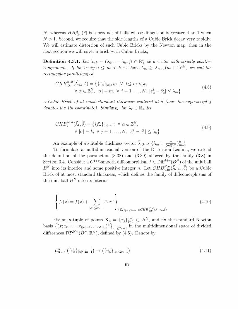
N , whereas HBst<2n(~r) is a product of balls whose dimension is greater than 1 when

N > 1. Second, we require that the side lengths of a Cubic Brick decay very rapidly.

We will estimate distortion of such Cubic Bricks by the Newton map, then in the

next section we will cover a brick with Cubic Bricks,

Definition 4.3.1. Let ~λ<k = (λ0, . . . , λk−1) ∈ Rk+ be a vector with strictly positive

components. If for every 0 ≤ m < k we have λm ≥ λm+1(m + 1)4N , we call the

rectangular parallelepiped

CHBN,st<k (~λ<k, ~δ) =

{{~εα}|α|<k : ∀ 0 ≤ m < k,

∀ α ∈ ZN+ , |α| = m, ∀ j = 1, . . . , N, |εj

α − δjα| ≤ λm

} (4.8)

a Cubic Brick of at most standard thickness centered at ~δ (here the superscript j

denotes the jth coordinate). Similarly, for λk ∈ R+ let

CHBN,stk (~λk, ~δ) =

{{~εα}|α|=k : ∀ α ∈ Z

N+ ,

∀ |α| = k, ∀ j = 1, . . . , N, |εjα − δj

α| ≤ λk

} (4.9)

An example of a suitable thickness vector ~λ<k is {λm = τ(m!)4N }k−1

m=0.

To formulate a multidimensional version of the Distortion Lemma, we extend

the definition of the parameters (3.38) and (3.39) allowed by the family (3.8) in

Section 3.4. Consider a C1+ρ-smooth diffeomorphism f ∈ Diff1+ρ(BN) of the unit ball

BN into its interior and some positive integer n. Let CHBN,st<2n (~λ<2n, ~δ) be a Cubic

Brick of at most standard thickness, which defines the family of diffeomorphisms of

the unit ball BN into its interior

f~ε(x) = f(x) +

∑

|α|≤2n−1

~εαxα

{~εα}|α|≤2n−1∈CHBN,st<2n (~λ<2n,~δ)

(4.10)

Fix an n-tuple of points Xn = {xj}n−1j=0 ⊂ BN , and fix the standard Newton

basis{(x; x0, . . . , x(|α|−1) (mod n))

α}

|α|≤2n−1in the multidimensional space of divided

differences DDN,n(BN , RN), defined by (4.5). Denote by

LNXn

:({~εα}|α|≤2n−1

)→

({~uα}|α|≤2n−1

)(4.11)

67

the Newton map that corresponds to rewriting an N -vector polynomial of degree

2n − 1 given in the basis {xα}|α|≤2n−1 in the Newton basis (4.5).

Consider the reparametrization of family (4.10) by the Newton parameters

f~u(2n−1),Xn(x) = f(x) +

∑

|α|≤2n−1

~uα(x; x0, . . . , x(|α|−1) (mod n))α. (4.12)

Denote by ~u(m) = ({~uα}|α|≤m) (respectively ~um = ({~uα}|α|=m)) the set of all

Newton parameters of degree at most m (respectively of degree exactly m).

In order to state the Discretization Lemma in the N -dimensional case, we have

to define the set of values of Newton parameters ~u(2n − 1) that are allowed by the

family (4.10) and the Cubic Brick (4.8).

Let Xk = {xj}k−1j=0 for 0 ≤ k ≤ n, and for convenience below let Xk = Xn for

n < k ≤ 2n − 1. Let

πN,u,Xk

<2n,≤k : W u<2n,N → W u,Xk

≤k,N and πN,u,Xk

<2n,k : W u<2n,N → W u,Xk

k,N

be the natural projection onto the space W u,Xk

≤k,N of N -vector polynomials in N variables

of degree k and the space W u,Xk

k,N of homogeneous N–vector polynomials in N variables

of degree k. As for N = 1, this projection depends only on Xk, not on Xn \ Xk.

Notice that the image of the Cubic Brick CHBN,st<2n (~λ<2n, ~δ) under the Newton

map LNXn

is a parallelepiped

PN,st<2n,Xn

(~λ<2n, ~δ) = LNXn

(CHBN,st<2n (~λ<2n, ~δ)), (4.13)

because the map LNXn

is linear.

We call the parallelepiped PN,st<2n,Xn

(~λ<2n, ~δ) the set of parameters allowed by the

family (4.10). Notice that the values of ~u(2n − 1) = (~u0, . . . , ~u2n−1) ∈ W u,Xn

<2n,N that

do not belong to PN,st<2n,Xn

(~λ<2n, ~δ) are of no interest for us, because they lie outside

of the range of the family (4.10) under consideration. Now we define the range of

allowed parameters ~u(k) ∈ W u,Xk

≤k,N for each 0 ≤ k ≤ 2n − 1.

Denote the images of the Cubic Brick CHBN,st<2n (~λ<2n, ~δ) under composition of

the Newton map LNXn

and the projections πN,u,Xk

<2n,≤k and πN,u,Xk

<2n,k by

PN,st<2n,≤k,Xk

(~λ<2n, ~δ) = πN,u,Xk

<2n,≤k ◦ LNXn

(CHBN,st<2n (~λ<2n, ~δ)) ⊂ W u

≤k,N

PN,st<2n,k,Xk

(~λ<2n, ~δ) = πN,u,Xk

<2n,k ◦ LNXn

(CHBN,st<2n (~λ<2n, ~δ)) ⊂ W u

k,N .(4.14)

68

It follows from the definition of the Newton map LNXn

that for each 0 ≤ k ≤2n − 1, the sets PN,st

<2n,≤k,Xk(~λ<2n, ~δ) and PN,st

<2n,k,Xk(~λ<2n, ~δ) are polyhedra depending

on Xk. We call PN,st<2n,≤k,Xk

(~λ<2n, ~δ) the set of parameters of order k allowed by the

family (4.10).

Similarly to the 1-dimensional Distortion Lemma from Section 3.4, its N -dimen-

sional generalization gives an estimate on the ratio of volumes of the polyhedra

PN,st<2n,≤k,Xk

(~λ<2n, ~δ) of allowed Newton parameters ~u(k) and the corresponding Cu-

bic Bricks CHBN,st<2n (~λ<2n, ~δ).

The Preliminary N-dimensional Distortion Lemma. Let Xn = {xj}n−1j=0 ⊂

BN be an n–tuple of points in the unit ball BN , and let LNXn

: W<2n,N → W u,Xn

<2n,N

be the Newton map (4.11) corresponding to the basis (4.5) for W u,Xn

<2n,N . Let ~λ<2n =

(λ0, . . . , λ2n−1) ∈ R2n+ be a vector with strictly positive components that defines a Cubic

Brick of CHBN,st<2n (~λ<2n, ~δ) of at most standard thickness and Leb≤k,N (resp. Lebk,N)

be the Lebesgue measure on the space W≤k,N (respectively Wk,N) of (respectively of

homogeneous) N -vector polynomials in N variable of degree k. Then for all 0 ≤ k ≤2n − 1, we have the volume ratio estimate

Lebk,N

(

PN,st<2n,k,Xk

(~λ<2n, ~δ))

Lebk,N

(

CHBN,stk (~λk, ~δ)

) ≤ 3N2n. (4.15)

Remark 4.3.2. As in the 1-dimensional case, the Newton map LNXn

is volume-

preserving, and hence the parallelepipeds PN,st<2n,Xn

(~λ<2n, ~δ) and CHBN,st<2n (~λ<2n, ~δ) have

the same volume. However, the estimate (4.15) concerns the volumes of projections of

these parallelepipeds. Since CHBN,st<2n (~λ<2n, ~δ) is a rectangular parallelepiped (aligned

with the coordinate axes) and PN,st<2n,Xn

(~λ<2n, ~δ) is not, the projections of the latter

set have larger volume according to the amount of shear in the Newton map. The

Distortion Lemma bounds the effect of the shear.

The lemma above will be proved in Part II of this paper in a more general form

required for the proof of the Main Result (Theorem 1.3.7). The other main ingredient

of Section 3.4, the Collection Lemma, proceeds in much the same way for general N

as it does for N = 1.

69

4.4 From a brick of at most standard thickness to

an admissible brick

In order to apply the method which we are developing in this paper to other problems

about generic properties of dynamical systems, we need to have a sufficiently rich

space of parameters (enough freedom to perturb). Various dynamical phenomena

have a “size” that is exponential in the period or number of iterations. Since we

perturb trajectories of length n with polynomials whose degree is proportional to n,

it seems essential to have a Hilbert Brick of parameters with sides decaying at most

exponentially in the period of the polynomials the respective parameters multiply.

That is, with the notations of Definition 1.3.1, we would like to have rn ≥ exp(−Cn)

for some C > 0. However, even for the 1-dimensional model, if we consider a brick of

parameters with exponentially decaying sides, then we cannot control the distortion

properties of the Newton map (see Remark 3.4.1).

In order to circumvent this problem, we do the following. Consider a Hilbert

Brick HBN(~r) of an admissible size ~r = {rk}∞k=0 (see Definition 1.3.1). Using Fubini’s

Reduction from Section 2.3 at the nth stage of induction over the period, we reduce

consideration of an infinite-dimensional Hilbert Brick HBN(~r) to a finite-dimensional

brick HBN<2n(~r).

Recall that HBN<2n(~r) belongs to the space of N -vector polynomials of degree

2n − 1, denoted by W<2n,N .

Definition 4.4.1. We call the Cubic Brick in W<2n,N of at most standard thickness

centered at a point ~δ<2n ∈ W<2n,N and associated to the brick HBN<2n(~r) the one

denoted by CHBN,st<2n (~λ<2n(~r), ~δ<2n) and defined by (4.8) where λm(~r) = rm/(m!)4N

and ~λ<2n(~r) = (λ0(~r), . . . , λ2n−1(~r)).

Remark 4.4.2. It follows from the nonincreasing property of the sequence rm (see

Definition 1.3.1) that

(m + 1)4Nλm+1(~r) = (m + 1)4N rm+1

((m + 1)!)4N≤ rm

(m!)4N= λm(~r), (4.16)

so that the Cubic Brick CHBN,st<2n (~λ<2n(~r), ~δ<2n) is of at most standard thickness.

We wish to cover the brick HBN<2n(~r) in W<2n,N by a collection of Cubic Bricks

{CHBN,st<2n (~λ<2n(~r), ~δ<2n)}~δ<2n∈G(~r) of at most standard thickness associated with it.

First we define a grid in W<2n,N on which the centers ~δ<2n should lie in order that

the Cubic Bricks fit together without overlap.

70

Recall that W<2n,N = ×2n−1m=0 Wm,N , dim Wm,N = ν(m,N), and denote η(k,N) =

∑km=0 ν(m,N). Let

Zη(2n−1,N)

2~λ<2n(~r)= Z

ν(0,N)2λ0(~r) × Z

ν(1,N)2λ1(~r) × · · · × Z

ν(2n−1,N)2λ2n−1(~r)

⊂ W0,N × W1,N × · · · × W2n−1,N = W<2n,N ,(4.17)

where Zν(m,N)2λm(~r) is the grid in R

ν(m,N) with spacing 2λm(~r) in each coordinate. Let

G(~r) ={

~δ<2n ∈ Zη(2n−1,N)

2~λ<2n(~r): HBN

<2n(~r) ∩ CHBN,st<2n (~λ<2n(~r), ~δ<2n) 6= ∅

}

. (4.18)

The Cubic Bricks with centers in G(~r) are the ones needed for

our covering:

HBN<2n(~r) ⊂ ∪~δ∈G(~r)CHBN,st

<2n (~λ<2n(~r), ~δ<2n). (4.19)

The Covering Lemma. The ratio of the volume of the covering (4.19) by Cubic

Bricks and the volume of the brick HBN<2n(~r) is bounded by e6N .

Proof: We claim that the covering (4.19) is contained in the slightly larger

brick HBN<2n({(1 + 2

√N

(m!)3N )rm}2n−1m=0 ). The amount that the covering extends beyond

HBN<2n(~r) in the direction of a given multiindex α with |α| = m is at most the di-

ameter in the α direction of one of the Cubic Bricks CHBN,st<2n (~λ<2n(~r), ~δ j

<2n), which

by Definition 4.4.1 is 2√

Nλm(~r) = 2√

Nrm/(m!)4N . Recall the definitions (2.27)

of HBN<2n(~r) and (1.12) of the norm used therein. In this norm, the diameter of

CHBN,st<2n (~λ<2n(~r), ~δ j

<2n) in the directions with |α| = m is 2√

Nrm/(m!)4N times the

square root of∑

|α|=m

(mα

)−1< (m!)N , from which our claim follows. The ratio of vol-

umes that we wish to bound is then at most∏2n−1

m=0 exp(2√

N/(m!)3N) ≤ e2e√

N < e6N .

Q.E.D.

Recall now that our main goal in the proof of Theorem 1.3.7 is to get an esti-

mate on the measure of the “bad” set of parameters (2.1) inside of the Hilbert Brick

HBN(~r). Using the Fubini reduction from Section 2.3, we know that it is sufficient to

get an estimate on the measure of the “bad” set in a finite-dimensional slice of the form

HBN<2n(~r)×{~ε≥2n} that is uniform over ~ε≥2n ∈ HBN

≥2n(~r) see (2.31-2.32). Notice now

that if we can prove that for each Cubic Brick slice CHBN,st<2n (~λ<2n(~r), ~δ<2n)×{~ε≥2n}

from the covering collection ~δ<2n ∈ G(~r) that the fraction of parameters in the slice

71

that are “bad” is uniformly small over ~δ<2n ∈ G(~r), then the same fraction is small

in the whole slice HBN<2n(~r) × {~ε≥2n}. (By the Covering Lemma, we must increase

the bound on the fraction of “bad” parameters only by the factor e6N , which is in-

dependent of n.) By the Fubini reduction, this shows that the measure of the “bad”

set in HBN(~r) is small too. Thus it is sufficient to prove the following estimate.

µN<2n,~r

(

Bn(C, δ, ρ,~r, f, ~ε≥2n) ∩ CHBN,st<2n (~λ<2n(~r), ~δ<2n)

)

µN<2n,~r

(

CHBN,st<2n (~λ<2n(~r), ~δ<2n)

)

≤ µ′n(C, δ, ρ,M1+ρ).

(4.20)

uniformly over all δ<2n ∈ J(~r) and so that∑∞

n=1 µ′n(C, δ, ρ,M1+ρ) converges for all

positive C, δ, ρ, and M1+ρ, and tends to zero as C tends to infinity.

4.5 The main estimate on the measure of “bad”

parameters

In this subsection we formulate the main theorem of the rest of the paper which

implies (the Main) Theorem 1.3.7. It will be proved in Part II of this paper.

Theorem 4.5.1. For any ρ > 0 and any diffeomorphism f ∈ Diff1+ρ(BN), consider

a Hilbert Brick HBN(~r) of an admissible size ~r with respect to f and the family of

analytic perturbations of f

{f~ε(x) = f(x) + φ~ε(x)}~ε∈HBN (~r) (4.21)

(see (1.10)) with the Lebesgue product probability measure µN~r (see (1.15)) associated

to HBN(~r).

Then for any positive integer n and any ~ε≥2n ∈ HBN≥2n(~r), consider a slice (2.27)

of the Hilbert Brick HBN(~r) of the form

HBN<2n(~r) × {~ε≥2n} ⊂ HBN

<2n(~r) × HBN≥2n(~r) = HBN(~r). (4.22)

Inside of this slice fix a grid point ~δ<2n ∈ G(~r), and consider the Cubic Brick

CHBN,st<2n (~λ<2n(~r), ~δ<2n) × {~ε≥2n} ⊂ HBN

<2n(~r) × {~ε≥2n}. (4.23)

from the covering (4.19) associated to the brick HBN<2n(~r).

72

Let f = f(~δ<2n,~ε≥2n) be a diffeomorphism corresponding to the center of the Cubic

Brick CHBN,st<2n (~λ<2n(~r), ~δ<2n) × {~ε≥2n}. Consider the family of diffeomorphisms

{f~ε<2n}~ε<2n∈CHBN,st

<2n (~λ<2n(~r),0) ⊃{f(~ε<2n+~δ<2n,~ε≥2n)}(~ε<2n+~δ<2n∈HBN

<2n(~r)∩CHBN,st<2n (~λ<2n(~r),~δ<2n).

(4.24)

Then for C ≥ 30/ρ log M1+ρ, the fraction of the measure of “bad” parameters

Bn(C, δ, ρ,~r, f, ~ε≥2n), defined in (2.32), inside CHBN,st<2n (~λ2n−1(~r), ~δ<2n)×{~ε≥2n} sat-

isfies the bound

µN<2n,~r

(

Bn(C, δ, ρ,~r, f, ~ε≥2n) ∩ CHBN,st<2n (~λ2n−1(~r), ~δ<2n)

)

µN<2n,~r

(

CHBN,st<2n (~λ2n−1(~r), ~δ<2n)

) ≤

24CeNn1+δ32nN2

M1+ρ max{M1+ρ, exp C/100}−n/2

(4.25)

The discussion from the end of the previous section shows that this theorem

implies (the Main) Theorem 1.3.7.

73

Appendix A: Properties of

hyperbolicity

In this paper we have quantified the hyperbolicity of periodic points in order to

bound from below the distance between periodic points of the same period. Recall

the definitions of γ(L), γn(x, f), and γn(f) from (1.6) and (1.7) and the text between

them. In this appendix we will prove Proposition 1.1.6, along with a result that

say that the hyperbolicity of a power of a linear operator is no smaller than the

hyperbolicity of the operator.

Proposition 1.1.6 follows immediately from the following lemma.

Lemma A.1. Given the hypotheses of Proposition 1.1.6, for every pair of distinct

period n points of f , say x = fn(x) 6= y = fn(y), the distance |x− y| between them is

at least (M−n(1+ρ)1+ρ γn(f))1/ρ.

Proof: Let v = (y − x)/|x − y|. Then

v =fn(y) − fn(x)

|x − y| =1

|x − y|

∫ |x−y|

0

d

dλfn(x + λv)dλ

=1

|x − y|

∫ |x−y|

0

dfn(x + λv)vdλ.

(A.1)

It follows that

1

|x − y|

∫ |x−y|

0

(dfn(x + λv)v − v)dλ = 0. (A.2)

Let w = dfn(x)v − v; by hypothesis |w| ≥ γn(f). Also,

|dfn(x + λv)v − v − w| = |(dfn(x + λv) − dfn(x))v|≤ ‖dfn(x + λv) − dfn(x)‖.

(A.3)

74

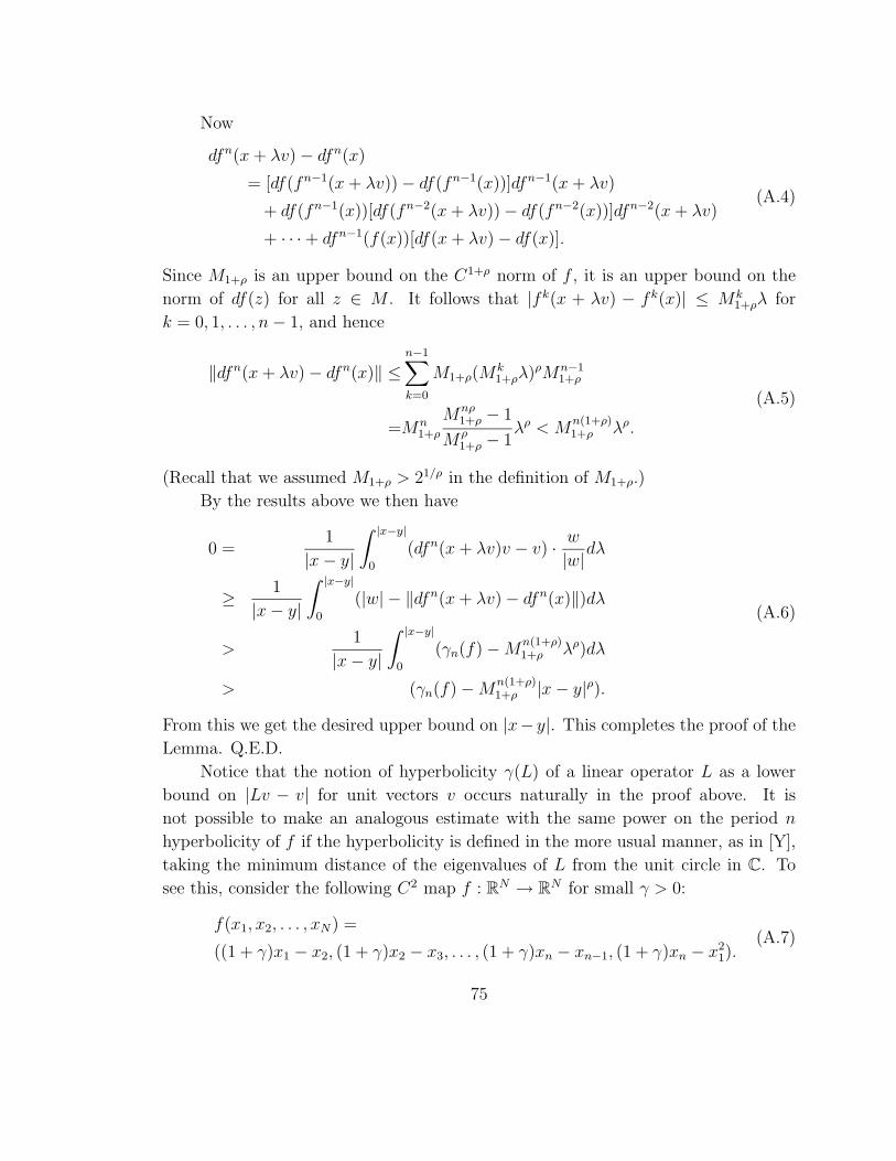
Now

dfn(x + λv) − dfn(x)

= [df(fn−1(x + λv)) − df(fn−1(x))]dfn−1(x + λv)

+ df(fn−1(x))[df(fn−2(x + λv)) − df(fn−2(x))]dfn−2(x + λv)

+ · · · + dfn−1(f(x))[df(x + λv) − df(x)].

(A.4)

Since M1+ρ is an upper bound on the C1+ρ norm of f , it is an upper bound on the

norm of df(z) for all z ∈ M . It follows that |fk(x + λv) − fk(x)| ≤ Mk1+ρλ for

k = 0, 1, . . . , n − 1, and hence

‖dfn(x + λv) − dfn(x)‖ ≤n−1∑

k=0

M1+ρ(Mk1+ρλ)ρMn−1

1+ρ

=Mn1+ρ

Mnρ1+ρ − 1

Mρ1+ρ − 1

λρ < Mn(1+ρ)1+ρ λρ.

(A.5)

(Recall that we assumed M1+ρ > 21/ρ in the definition of M1+ρ.)

By the results above we then have

0 =1

|x − y|

∫ |x−y|

0

(dfn(x + λv)v − v) · w

|w|dλ

≥ 1

|x − y|

∫ |x−y|

0

(|w| − ‖dfn(x + λv) − dfn(x)‖)dλ

>1

|x − y|

∫ |x−y|

0

(γn(f) − Mn(1+ρ)1+ρ λρ)dλ

> (γn(f) − Mn(1+ρ)1+ρ |x − y|ρ).

(A.6)

From this we get the desired upper bound on |x− y|. This completes the proof of the

Lemma. Q.E.D.

Notice that the notion of hyperbolicity γ(L) of a linear operator L as a lower

bound on |Lv − v| for unit vectors v occurs naturally in the proof above. It is

not possible to make an analogous estimate with the same power on the period n

hyperbolicity of f if the hyperbolicity is defined in the more usual manner, as in [Y],

taking the minimum distance of the eigenvalues of L from the unit circle in C. To

see this, consider the following C2 map f : RN → R

N for small γ > 0:

f(x1, x2, . . . , xN) =

((1 + γ)x1 − x2, (1 + γ)x2 − x3, . . . , (1 + γ)xn − xn−1, (1 + γ)xn − x21).

(A.7)

75

Notice that f has two nearby fixed points, 0 and (γN , γN+1, . . . , γ2N−1), that are

within roughly γN of each other. Notice also that df(0) is upper triangular and hence

all N of its eigenvalues are 1 + γ, so that by the eigenvalue notion of hyperbolicity 0

is an (n, γ)-hyperbolic fixed point of f . (Though df has eigenvalues closer to the unit

circle at the other fixed point, they are still much farther away than γN for large N .)

On the other hand, for v = (1, γ, . . . , γN−1) we have |v| slightly larger than 1 while

|Lv − v| = |(0, 0, . . . , γN)| = γN , (A.8)

so that our notion of hyperbolicity is commensurate with the spacing between the

fixed points.

To this point, when using the hyperbolicity of a linear operator L, it has only

been important that |Lv−v| not be small for unit vectors v. The reason for estimating

from below |Lv − exp(2πiφ)v| for φ ∈ [0, 1) in (1.6) is that the hyperbolicity of L

will be a lower bound on the hyperbolicity of Lk for positive integers k. In terms of

diffeomorphisms, this estimate gives a bound on how close points of period nk can lie

to a hyperbolic point of period n. For the eigenvalue-based notion of hyperbolicity,

the estimate is trivial, but for our notion it must be proved.

Lemma A.2. For every linear operator L : CN → C

N and k ∈ Z+, we have γ(Lk) ≥

γ(L).

Proof: Suppose γ(Lk) < γ(L); then for some φ ∈ [0, 1) and unit vector v ∈ CN

we have |Lkv − exp(2πiφ)v| < γ(L). Without loss of generality we may assume

that φ = 0; otherwise replace L with exp(−2πiφ/k)L, so that γ(L) and γ(Lk) are

unaffected and |Lkv − v| < γ(L). Let ω = exp(2πi/k), and for j = 0, 1, . . . , k − 1 let

uj = v + ωjLv + ω2jL2v + · · · + ω(k−1)jLk−1v. (A.9)

Notice that u0 + u1 + · · · + uk−1 = kv, and since v is a unit vector we must have

|uj| ≥ 1 for some j. But

Luj − ω−juj = Lv − ω−jv + ωjL2v − Lv + · · ·ω(k−1)jLkv − ω(k−2)jLk−1v

= ω(k−1)jLkv − ω−jv = ω−j(Lv − v),(A.10)

the last step because ω is a k-th root of unity. This yields |Luj −ω−juj| = |Lv− v| <

γ(L), contradicting the definition of γ(L). This completes the proof of the lemma.

Q.E.D.

The next lemma is a simple estimate on how much a small perturbation of a

linear operator can change its hyperbolicity.

76

Lemma A.3. For any pair of linear operators L and ∆ of RN into itself, hyperbolicity

satisfies the estimate

γ(L + ∆) ≥ γ(L) − ‖∆‖. (A.11)

Proof: By the definition of hyperbolicity,

γ(L + ∆) = infφ∈[0,1)

inf‖v‖=1

|(L + ∆)v − exp(2πiφ)v|. (A.12)

By triangle inequality, for all v ∈ RN ,

|(L + ∆)v − exp(2πiφ)v| ≥ |Lv − exp(2πiφ)v| − |∆v|. (A.13)

This implies the statement of the lemma. Q.E.D.

The following lemma generalizes the previous two lemmas. The proof is very

similar to that of Lemma A.2, but we need to be a bit more careful.

Lemma A.4. For all linear operators L,L1, L2, . . . , Lk : CN → C

N ,

γ(LkLk−1 · · ·L1) ≥ γ(L) −k∑

j=1

‖L − Lj‖. (A.14)

Proof: Choose v0 ∈ CN and φ ∈ R such that

|LkLk−1 · · ·L1v0 − eiφv0| = γ(LkLk−1 · · ·L1)|v0|. (A.15)

Let v1 = L1v0, v2 = L2L1v0, . . . , vk = LkLk−1 · · ·L1v0. For j = 0, 1, . . . , k − 1 let

ωj = ei(−φ+2πj)/k (A.16)

and

uj = v0 + ωjv1 + ω2j v2 + · · · + ωk−1

j vk−1. (A.17)

Choose ℓ for which |vℓ| = max(|v0|, |v1|, . . . , |vk−1|), and notice that

k−1∑

j=0

ω−ℓj uj = kvℓ. (A.18)

Thus there exists j such that

|uj| ≥ |vℓ| = max(|v0|, |v1|, . . . , |vk−1|). (A.19)

77

Then we have

γ(L) ≤ |Luj − ω−1j uj|/|uj|

=| − ω−1

j v0 + Lv0 − v1 + Lωjv1 − ωjv2 + · · · + Lωk−1j vk−1|

|uj|

=|ωk−1

j (vk − eiφv0) + (L − L1)v0 + (L − L2)ωjv1 + · · · (L − Lk)ωk−1j vk−1|

|uj|

≤γ(LkLk−1 · · ·L1)|v0| + ‖L − L1‖|v0| + ‖L − L2‖|v1| + · · · + ‖L − Lk‖|vk−1||uj|

≤γ(LkLk−1 · · ·L1) + ‖L − L1‖ + ‖L − L2‖ + · · · + ‖L − Lk‖,

which is equivalent to the desired inequality. Q.E.D.

Proposition A.5. Let r ≤ 1 ≤ K be positive numbers and A,B be linear operators

of RN into itself given by N ×N matrices from MN(R) with real entries. Consider an

N2-parameter family {AU = A + UB}U∈CN2(r), where CN2

(r) is the cube in MN(R)

whose entries are bounded in absolute value by r. Suppose that ‖B‖, ‖B−1‖ ≤ K.

Then for the Lebesgue product probability measure µr,N2 on the cube CN2(r) and all

0 < γ ≤ min(r, 1), we have

µr,N2

{

U ∈ CN2

(r) : γ(AU) ≤ γ}

≤ C(N)K2N2γ

r2, (A.20)

where the constant C(N) depends only on N .

Proof: For 0 < γ ≤ 1 and φ ∈ [0, 1), define the sets of non-γ-hyperbolic matrices

by

NHγN(R) = {L ∈ MN(R) : γ(L) ≤ γ},

NHγ,φN (R) = {L ∈ MN(R) : inf

|v|=1|(L − exp(2πiφ)v| ≤ γ}. (A.21)

Then

NHγN(R) = ∪φ∈[0,1)NHγ,φ

N (R). (A.22)

We claim that

NHγN(R) ⊂ ∪j=0,...,[5/γ]−1NH

2γ,j/[5/γ]N (R). (A.23)

78

Indeed, suppose that L ∈ NHγN(R). Then for some number φ ∈ [0, 1) and vector

v ∈ RN with |v| = 1, we have |(L− exp(2πiφ))v| ≤ γ. Let j be the nearest integer to

[5/γ]φ and let φγ = j/[5/γ]; then φ − φγ ≤ 1/(2(5/γ − 1)) < γ/(2π). Thus

|(L − exp(2πiφγ))v| ≤|(L − exp(2πiφ))v| + | exp(2πiφ) − exp(2πiφγ)| ≤ 2γ

(A.24)

and L ∈ NH2γ,j/[π/γ+1]N (R) as claimed.

Next, we claim that every matrix in NH2γ,j/[5/γ]N (R) lies within 2γ of a matrix in

NH0,j/[5/γ]N (R), where we use the Euclidean (RN2

) norm on MN(R) (not the matrix

norm). Consider L ∈ NH2γ,j/[5/γ]N (R), φ ∈ [0, 1), and v ∈ R

N with |v| = 1 and

|(L − exp(2πij/[5/γ]))v| ≤ 2γ. Let w = (L − exp(2πij/[5/γ]))v and let M ∈ MN(R)

be the matrix whose kth row is wkv, where wk is the kth coordinate of w. Then the

Euclidean norm of M is |w| ≤ 2γ and Mv = w, so that (L−M−exp(2πij/[5/γ]))v = 0

and hence L − M ∈ NH0,j/[5/γ]N (R).

We complete the estimate (A.20) by estimating for each j the number of γ-balls

needed to cover NH0,j/[5/γ]N (R) within an appropriate bounded domain. It then follows

from the previous paragraph that if we inflate each of these balls to the concentric

ball of radius 3γ, the collection of larger balls will cover NH2γ,j/[5/γ]N (R), and from

the paragraph before that the union over j of these covers will then cover NHγN(R).

To this end, we show that each NH0,j/[5/γ]N (R) is a real algebraic set and compute

its codimension1. Then we will apply an estimate of Yomdin [Y] on the number of

γ-balls necessary to cover a given algebraic set by polynomials of known degree.

Notice that

NH0,φN (R) = {L ∈ MN(R) : det(L − exp(2πiφ)Id) = 0}. (A.25)

We split into the two cases exp(2πiφ) ∈ R (that is, φ = 0 or 1/2) and exp(2πiφ) /∈ R.

In the first case, the equation det(L ± Id) = 0 is a polynomial of degree N in the

entries of L, so NH0,0N (R) and NH

0,1/2N (R) are real algebraic sets defined by a single

polynomial of degree N .

In the second case, decompose the equation det(L − exp(2πiφ)Id) = 0 into two

parts: Re[det(L − exp(2πiφ)Id)] = 0 and Im[det(L − exp(2πiφ)Id)] = 0. Each

part is given by a real polynomial of degree N . Furthermore, these two polyno-

mials are algebraically independent, since otherwise Re[det(L − exp(2πiφ)Id)] and

Im[det(L − exp(2πiφ)Id)] would satisfy some polynomial relationship and, thus,

1Unfortunately NH0N (R), in contrast to NH

0,j/[5/γ]N (R), is not algebraic

79

det(L− exp(2πiφ)Id) would take on values only in some real algebraic subset of

the complex plane. However, for N ≥ 2 (which is necessary for complex eigenvalues),

by considering real diagonal matrices L we see that the values of det(L−exp(2πiφ)Id)

contain an open set in C. Therefore, NH0,φN (R) is a real algebraic set given by two

algebraically independent polynomials of degree N .

Covering Lemma for Algebraic Sets ([Y], Lemma 4.6) Let V ⊂ Rm be an

algebraic set given by k algebraically independent polynomials p1, . . . , pk of degrees

d1, . . . , dk respectively, i.e. V = {x ∈ Rm : p1(x) = 0, . . . , pk(x) = 0}. Let Cm

A (s) be

the cube in Rm with side 2s centered at some point A. Then for γ ≤ s, the number of

γ-balls necessary to cover V ∩ CmA (s) does not exceed C(D,m) (2s/γ)m−k, where the

constant C(D,m) depends only on the dimension m and product of degrees D =∏

i di.

Remark A.6. Some additional arguments based on Bezout’s Theorem give an upper

estimate of C(D,m) by 2mD for γ sufficiently small.

To complete the proof of Proposition A.5, we apply the Covering Lemma for

Algebraic Sets to each NH0,j/[5/γ](R), where j = 0, . . . , [5/γ] − 1, with m = N2,

s = Kr, and A as in the statement of the proposition. (Notice that if U ∈ CN2(r)

then A + UB ∈ CN2

A (Kr), so we need only cover the part of NH0,j/[5/γ](R) lying in

the latter set.) In the case that j/[5/γ] = 0 or 1/2, we have k = 1, d1 = N , and

D = N , so the number of covering γ-balls is bounded by C(N,N 2)(2Kr/γ)N2−1. In

the case of other j, we have k = 2, d1 = d2 = N , and D = N2, so the number of

covering γ-balls is bounded by C(N2, N2)(2Kr/γ)N2−2. The number of j’s of the

second type is less than 5/γ. Combining all these estimates along with (A.23) we get

that NHγ(R) ∩ CN2

A (Kr) can be covered by C(N2, N2)(2 + 5/(2Kr))(2Kr/γ)N2−1

balls of radius 3γ.

Finally, notice that the preimage of a ball of radius 3γ under the map U 7→ A +

UB is contained in a ball of radius 3Kγ, whose µr,N2-measure is less than (3Kγ/r)N2.

Therefore the total measure of 3Kγ-balls needed to cover the set {U ∈ CN2(r) :

γ(A + UB) ≤ γ} is at most C(N)K2N2γ/r2, where the constant C(N) depends only

on N . Q.E.D.

80

Appendix B: Orthogonal

transformations of RN and the

spaces of homogeneous polynomials

In this appendix, we prove that the scalar product (1.12) in the space Wk,N of homo-

geneous N -vector polynomials of degree k in N variables is invariant with respect to

orthogonal transformations of RN .

Lemma B.1. Let x ∈ RN be given by N coordinates x = (x1, . . . , xN). For k ∈ Z+,

consider homogeneous polynomials pk(x) =∑

|α|=k ~εαxα ∈ Wk,N in N variables, where

xα = xα11 . . . xαN

N . Let O ∈ SO(N) be an orthogonal transformation of RN . Denote

by x′ = (x′1, . . . , x

′N) the new coordinate system induced by the relation x = Ox′.

Write p′k(x′) = pk(Ox′) =

∑

|α|=k ~ε ′α (x′)α in the new coordinate system. Then for all

{~εα}|α|=k and {~να}|α|=k,

∑

|α|=k

(k

α

)−1

〈~εα, ~να〉 =∑

|α|=k

(k

α

)−1

〈~ε ′α, ~ν ′

α〉. (B.1)

Proof: For this lemma it will be helpful to use a different notation for monomials.

Given a k-tuple β = (β1, . . . , βk) ∈ {1, 2, . . . , N}k, define x(β) = xβ1xβ2 · · ·xβk. Notice

that x(β) = xα where αi is the number of indices j for which βj = i. Write α(β) for

the multiindex corresponding in this manner to the k-tuple β, and notice that for

each multiindex α there are(

kα

)different k-tuples β for which α(β) = α. Let |β| = k.

Given a polynomial pk as in the statement of the lemma, we can write pk(x) =∑

|β|=k ~ε(β)x(β), where ~ε(β) =

(kα

)−1~εα(β). We can also rewrite the scalar product as

follows:

∑

|α|=k

(k

α

)−1

〈~εα, ~να〉 =∑

|β|=k

〈~ε(β), ~ν(β)〉. (B.2)

81

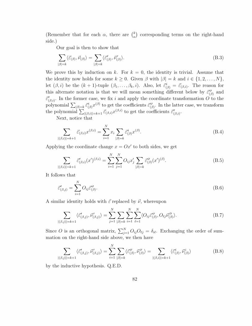
(Remember that for each α, there are(

kα

)corresponding terms on the right-hand

side.)

Our goal is then to show that∑

|β|=k

〈~ε(β), ~ν(β)〉 =∑

|β|=k

〈~ε ′(β), ~ν

′(β)〉. (B.3)

We prove this by induction on k. For k = 0, the identity is trivial. Assume that

the identity now holds for some k ≥ 0. Given β with |β| = k and i ∈ {1, 2, . . . , N},let (β, i) be the (k + 1)-tuple (β1, . . . , βk, i). Also, let ~ε i

(β) = ~ε(β,i). The reason for

this alternate notation is that we will mean something different below by ~ε i′(β) and

~ε ′(β,i). In the former case, we fix i and apply the coordinate transformation O to the

polynomial∑

|β|=k ~ε i(β)x

(β) to get the coefficients ~ε i′(β). In the latter case, we transform

the polynomial∑

|(β,i)|=k+1 ~ε(β,i)x(β,i) to get the coefficients ~ε ′

(β,i).

Next, notice that

∑

|(β,i)|=k+1

~ε(β,i)x(β,i) =

N∑

i=1

xi

∑

|β|=k

~ε i(β)x

(β). (B.4)

Applying the coordinate change x = Ox′ to both sides, we get

∑

|(β,i)|=k+1

~ε ′(β,i)(x

′)(β,i) =N∑

i=1

N∑

j=1

Oijx′j

∑

|β|=k

~ε i′(β)(x

′)(β). (B.5)

It follows that

~ε ′(β,j) =

N∑

i=1

Oij~εi′(β). (B.6)

A similar identity holds with ~ε replaced by ~ν, whereupon

∑

|(β,j)|=k+1

〈~ε ′(β,j), ~ν

′(β,j)〉 =

N∑

j=1

∑

|β|=k

N∑

i=1

N∑

ℓ=1

〈Oij~εi′(β), Oℓj~ν

ℓ′(β)〉. (B.7)

Since O is an orthogonal matrix,∑N

j=1 OijOℓj = δiℓ. Exchanging the order of sum-

mation on the right-hand side above, we then have

∑

|(β,j)|=k+1

〈~ε ′(β,j), ~ν

′(β,j)〉 =

N∑

i=1

∑

|β|=k

〈~ε i′(β), ~ν

i′(β)〉 =

∑

|(β,i)|=k+1

〈~ε i(β), ~ν

i(β)〉 (B.8)

by the inductive hypothesis. Q.E.D.

82

Appendix C: Embedding of the

space of diffeomorphisms of a

compact manifold Diffr(M) into

that of an open set in a Euclidean

space

In this appendix, we describe how to extend an perturb a diffeomorphism of a com-

pact manifold embedded into a Euclidean space, and what conditions we need to

ensure that the results of Sacker [Sac] and Fenichel [F] about persistence of invariant

manifolds apply.

Recall that M is a smooth (C∞) compact manifold, and let f be a diffeomor-

phism in Diffr(M). First we consider a manifold M = M × [0, 1]/ ∼, where the

equivalence relation is defined by (x, 1) ∼ (f(x), 0) for all x ∈ M . Then M is as

smooth as f is and carries a naturally defined vector field Xf whose time one map,

restricted to M ×{0}, coincides with f . Such a construction is usually called suspen-

sion. Now we embed M into the interior of the closed unit ball BN+1 ⊂ RN+1 in such

a way that M ×{0} embeds into an N -dimensional subspace. Given a compact man-

ifold M of dimension D, for N + 1 > 2D the Whitney Embedding Theorem (see e.g.

[GG]) says that a generic smooth map from M to RN+1 is an embedding, i.e., a dif-

feomorphism between M and its image. Fix coordinates in RN+1. Consider a smooth

map E ′ : M → BN+1 such that E ′(M × {0}) ⊂ RN × {0}, the hyperplane where the

last coordinate is zero. By the Whitney Embedding Theorem, we can choose a small

perturbation E of E ′ such that E is an embedding of M . Since E(M×{0}) is close to

RN × {0}, we can change coordinates in R

N+1 so that E(M × {0}) ⊂ RN × {0} with

a new coordinate system. The mapping x 7→ E(x, 0) then provides an embedding

83

of M into the hyperplane in RN+1 where the last coordinate equals zero, which we

identify with RN . To simplify notation, we identify M and M with their images, so

that M and M become submanifolds of RN+1 and R

N respectively, with M × {0} a

submanifold of M .

Before we present a way to extend a vector field on M to its tube neighbor-

hood, we need to recall notion of a k-normally hyperbolic manifold. Recall that the

minimum norm m(L) of a linear transformation L is defined as

m(L) = inf{|Lx| : |x| = 1}.

When L is invertible, m(L) = ‖L−1‖−1. Fix t > 0. Let X be a Cr smooth vector

field on RN+1 and X t be the time t map along trajectories of X. Let TMR

N+1 be

the tangent bundle of RN+1 over M . Suppose we have a dX t-invariant splitting into

three subspaces

TMRN+1 = W u

⊕

TM⊕

W s,

i.e. for any y ∈ RN+1 we have dX t(y)W s

y = W sXt(y) and dX t(y)W u

y = W uXt(y). More-

over, for some C > 0 and λ > 1 we have |dX t(y)v| ≥ Cλt|v| for all y ∈ M , all v ∈ W uy

(respectively W sy ), and all t ≥ 0 (respectively t ≤ 0). Denote

d(X t)s(y) = dX t(y)|W s , d(X t)u(y) = dX t(y)|W u , d(X t)c(y) = dX t(y)|TyM .

Let 0 ≤ k ≤ r. We say that the vector field X is k-normally hyperbolic at M if there

is such a splitting that for all y ∈ M we have:

m(d(X t)u(y)) > ‖d(X t)c(y)‖k and m(d(X t)c(y))k > ‖d(X t)s(y)‖.

Notice that if X t is k-normally hyperbolic for small enough t, then it is k-normally

hyperbolic for all positive t.

Let T ⊂ RN+1 be a closed neighborhood of M , chosen sufficiently small that

there is a well-defined projection π : T → M for which π(x) is the closest point in M

to x. Then for each y ∈ M , by the Implicit Function Theorem, π−1(y) is an (N −D)-

dimensional disk. Then we can extend each vector field X on M to a vector field X on

T so that the component tangent to π−1(y) is directed toward y and is r-dominated

by the orthogonal one, meaning that the vector field X is r-normally hyperbolic at

M . Such an extension is possible because M is compact and one can keep increasing

the “strength” of attraction toward M by X until r-normal hyperbolicity is attained.

Consider the Poincare return map of Xf from T = T ∩{BN × {0}

}into BN ×

{0}, which is well-defined by the construction. Denote this map by F . The vector

84

field Xf is directed so that F maps T strictly inside itself. Now we shall use r-

normally hyperbolicity of X to construct an Artin-Mazur approximation fε of f via

approximating X and relying on persistence of M for the Poincare return map of X .

Now the closed neighborhood T of M can be considered as a subset of RN and

can be chosen sufficiently small that there is a well-defined projection π : T → M for

which π(x) is the closest point in M to x. Every small perturbation Fε ∈ Cr(T ) of F

can be suspended to a vector field Xfεclose to Xf . Then by Fenichel’s Theorem [F],

for ε sufficiently small Fε has an invariant manifold Mε ⊂ T for which π|Mεis a Cr

diffeomorphism from Mε to M . Then to such an Fε we can associate a diffeomorphism

fε ∈ Diffr(M) by letting

fε(y) = π(Fε(π|−1Mε

(y))).

Notice that the periodic points of Fε all lie on Mε and are in one-to-one cor-

respondence with the periodic points of fε. Furthermore, because fε and Fε|Mεare

conjugate, the hyperbolicity of each periodic orbit is the same for either map. Thus

any estimate on Pn(Fε) or γn(Fε) applies also to fε.

85

Appendix D: Pathological

examples of decay of product of

distances of recurrent trajectories

In this Appendix we present two types orbits of a horseshoe diffeomorphism that

show that with the methods we have in this paper, the estimate exp(Cn1+δ) on the

growth of the number of periodic points (the Main Theorem from Section 1.3) can-

not be improved to exp(Cn(log n)δ) for any real number δ. More exactly, the Shift

Theorem, stated in Section 3.5, is crucial to split all almost periodic trajectories into

classes as in (3.12). In Section 3.5, we outline the proof of this Theorem and it might

be helpful to review the strategy presented there, especially, the last remark right

before Section 3.5.1. Suppose that we now set γn(C, δ), which is roughly the inverse

of the bound we get on the number of periodic points, equal to exp(−Cn(log n)δ). In

Example 2,we construct a trajectory that for an infinite number of periods n is non-

simple, has no leading saddles, and no close returns (gaps), as defined in Section 3.5.

Thus for such slowly decaying γn(C, δ), we can’t deal with these kind of trajectories

with our methods.

First we give an example that shows more simply that the product of distances

along a period n orbit can be of order exp(−Cn log n) even though the closest return

along the orbit is of order exp(−Cn).

Example D.1. Consider the sequence of periodic orbits of a horseshoe map

86

with symbolic dynamics

S0 = 1

S1 = 0

S2 = 01

S3 = 010

S4 = 01001

S5 = 01001010

S6 = 0100101001001... .

Each sequence is the concatenation of the previous two sequences; it can also be

generated from the previous sequence by the substitution rules 0 → 01 and 1 → 0.

The number of symbols in Sn is the nth Fibonacci number Fn.

Notice also that

Sn = Sn−1Sn−2

= Sn−2Sn−3Sn−2

= Sn−3Sn−4Sn−3Sn−3Sn−4

= Sn−4Sn−5Sn−4Sn−4Sn−5Sn−4Sn−5Sn−4

= . . . .

More formally, the sequence Sn can be generated from Sk for any 0 ≤ k ≤ n by replac-

ing each 0 in Sk by Sn−k+1 and each 1 by Sn−k. We refer below to this decomposition

of Sn into copies of Sn−k and Sn−k+1 as “decomposition k”.

Every three symbol subsequence of Sn is either 010, 100, 001, or 101. Fur-

thermore, regarding each Sn as a cyclic sequence, each of the four triplets above

occurs at least once in S4, at least once in S5, at least twice in S6, and in gen-

eral at least Fn−4 times in Sn for n ≥ 4. The importance of this observation

below will be that in decomposition k for 4 ≤ k ≤ n, each of the substrings

Sn−k+1Sn−kSn−k+1, Sn−kSn−k+1Sn−k+1, Sn−k+1Sn−k+1Sn−k, and Sn−kSn−k+1Sn−k oc-

curs at least Fk−4 times.

Now let x0, x1, . . . , xp−1 be points in the periodic orbit with symbolic dynamics

Sn, where p = Fn is the length of Sn. No matter where the symbolic sequence of x0

87

starts within Sn, we claim that for n sufficiently large,

p−1∏

j=1

|x0 − xj| ≤ e(c1−c2n)p ≤ ec1p−c3p log p

for some positive constants c1, c2, c3 independent of n. The latter inequality follows

from the fact that p ≤ 2n, so it remains to prove the first inequality.

Assume that the distance between any two points in the nonwandering set is

at most 1. Say the symbolic sequence of x0 starts at the mth symbol of Sn. If for

some positive integer q, the block of 2q − 1 symbols centered at the mth symbol is

repeated centered at the ℓth symbol, then the distance between the points x0 and

xℓ−m is bounded above by e−cq for an appropriate positive constants c. Here the index

ℓ − m is taken modulo p.

Now for 4 ≤ k ≤ n, in decomposition k the mth symbol in Sn lies in a copy of

either Sn−k or Sn−k+1, which in turn lies in the middle of one of the four substrings

Sn−k+1Sn−kSn−k+1, Sn−kSn−k+1Sn−k+1, Sn−k+1Sn−k+1Sn−k, and Sn−kSn−k+1Sn−k de-

scribed above. Each such substring occurs at least Fk−4 times in Sn, and all but one of

these occurrences contributes a factor of at most e−cFn−k to the product of distances

|x0 − xj|. Therefore for n ≥ 6,

p−1∏

j=1

|x0 − xj| ≤n∏

k=6

(e−cFn−k)Fk−4−Fk−5

= e−c∑n

k=6 Fn−kFk−6

≤ e−c(n−5)Fn/F8

= ec(5−n)p/34.

(The estimate Fn−kFk−6 ≥ Fn/F8 can be proved by induction, but heuristically this

type of estimate follows from the fact that Fn is approximately an exponential function

of n.)

Example D.2. Consider now the aperiodic nonwandering orbit of the horseshoe

map whose symbolic dynamics are given as follows. Given a sequence of positive

integers k1, k2, . . ., let S0 = 0 and Sn = 1Sn−1Sn−1 · · ·Sn−11 where Sn−1 occurs 2kn+1

consecutive times. For example, if kn = n then

S0 = 0

S1 = 10001

S2 = 110001100011000110001100011... .

88

Each sequence is symmetric, and for n ≥ 1, each Sn contains a copy of Sn−1 at its

center. Let Ln be the length of Sn; then L0 = 1 and Ln = (2kn + 1)Ln−1 + 2 for

n ≥ 1. One can easily check that k1k2 · · · kn ≤ Ln ≤ 5nk1k2 · · · kn.

Let x0 be the point on the nonwandering set whose symbolic sequence has middle

Ln symbols Sn for each n ≥ 0. By symmetry, to estimate the product of distances

|x0 − xj| as j goes from 1 to Ln − 1, we can estimate the product as j goes from

−(Ln − 1) to Ln − 1, excluding j = 0, and take the square root of the latter estimate.

As in the previous example, let c be a positive constant such that |x0−xj| ≤ e−cq,

where q is the largest positive integer for which the middle 2q − 1 symbols of the

sequences for x0 and xj agree, or q = 0 if their middle symbols do not agree. Then

for all n ≥ 1 and −kn ≤ m ≤ kn we have |x0 − xmLn−1 | ≤ e−c(kn−|m|+1/2)Ln−1 . The

square root of the product of these upper bounds, excluding m = 0, is

kn∏

m=1

e−c(kn−m+1/2)Ln−1 = e−ck2nLn−1/2 ≤ e−cknLn/10.

Here we used the inequality 5knLn−1 ≥ (2kn + 1)Ln−1 + 2 = Ln.

In addition, for n and m as above and all −kn−1 ≤ p ≤ kn−1 we have |x0 −xmLn−1+pLn−2| ≤ e−c(kn−1−|p|+1/2)Ln−2 . The square root of the product of these upper

bounds, excluding p = 0, is

kn∏

m=−kn

kn−1∏

p=1

e−c(kn−1−p+1/2)Ln−2 = e−c(2kn+1)k2n−1Ln−2/2

≤ e−c(2kn+1)kn−1(Ln−1+1)/12.

Here we used the inequality 6kn−1Ln−2 ≥ (2kn−2 + 1)Ln−2 + 3 = Ln−1 + 1. Then in

turn we can say (2kn +1)(Ln−1 +1) ≥ (2kn +1)Ln−1 +3 = Ln +1, so that the bound

on the product above can be replaced by e−ckn−1Ln/12.

In a similar manner, we can bound above another set of terms contributing to

the product of distances |x0 − xj| by e−ckn−ℓLn/12 for ℓ = 2, 3, . . . , n − 1. Multiplying

all these bounds together we conclude that

Ln−1∏

j=1

|x0 − xj| ≤ e−c(k1+k2+···+kn)Ln/12.

Notice that if kn = k independent of n, then Ln ∼ (2k + 1)n and k1 + k2 + · · ·+ kn =

nk ∼ log Ln. Thus we get an estimate similar to Example 1.

89

If kn = nα, then log Ln ∼ n log n and hence k1 + k2 + · · · + kn ∼ nα+1 ∼(log Ln)α+1, loosely speaking. The closest returns to x0 are of the form − log |x0 −xLn

| ∼ kn+1Ln ∼ Ln(log Ln)α, loosely speaking again. Thus if we attempt to apply the

Inductive Hypothesis with γj(C, δ) = exp(−Cj(log j)δ), this example with α = δ−1/2

shows that for the product of distances along a hyperbolic trajectory can be smaller

than any fixed power of γj(C, δ) for arbitrarily large j = Ln, despite the fact that

the closest return over j iterations is larger than any fixed power of γj(C, δ) for j

sufficiently large.

90

References

[A] A. Arnold, Problems of Arnold’s seminar, 1989.

[AM] M. Artin & B. Mazur, On periodic orbits, Ann. Math. 81 (1965), 82–99.

[F] N. Fenichel, Persistence and smoothness of invariant manifolds for flows,Indiana Univ. Math. J. 21 (1971), 193–226.

[GG] M. Golubitsky and V. Guillemin, Stable Mappings and Their Singularities,Springer-Verlag (1973).

[GST1] S. Gonchenko, L. Shil’nikov, D. Turaev, On models with non-rough Poincarehomoclinic curves, Physica D 62 (1993), 1–14.

[GST2] S. Gonchenko, L. Shil’nikov, D. Turaev, Homoclinic tangencies of an arbitraryorder in Newhouse regions, (Russian) Dynamical systems (Russian) (Moscow,1998), 69–128, Itogi Nauki Tekh. Ser. Sovrem. Mat. Prilozh. Temat. Obz.,67, Vseross. Inst. Nauchn. i Tekhn. Inform. (VINITI), Moscow, 1999.

[GK] A. Gorodetski, V. Kaloshin, How often surface diffeomorphisms have in-finitely many sinks and hyperbolicity of periodic points near a homoclinictangency, preprint, 2004, 99pp, www.its.caltech.edu/ tilde kaloshin .

[GY] A. Grigoriev, S. Yakovenko, Topology of Generic Multijet Preimages andBlow-up via Newton Interpolation, J. of Diff. Equations, 150, 349-362,(1998).

[G] M. Gromov, On entropy of holomorphic maps, preprint.

[HSY] B. Hunt, T. Sauer, J. Yorke, Prevalence: a translation-invariant almost everyfor infinite dimensional spaces, Bull. Amer. Math. Soc. 27 (1992), 217–238;Prevalence: an addendum, Bull. Amer. Math. Soc. 28 (1993), 306–307.

[K1] V. Kaloshin, An extension of the Artin-Mazur Theorem, Ann. Math. 150(1999), 729–741.

[K2] V. Kaloshin, Generic diffeomorphisms with superexponential growth of num-ber of periodic orbits, Comm in Math Phys, 211, (2000), no.1, 253-271.

91

[K3] V. Kaloshin, Some prevalent properties of smooth dynamical systems, Tr.Math. Inst. Steklova 213 (1997), 123–151.

[K4] V. Kaloshin, Stretched exponential estimate on growth of the number of peri-odic points for prevalent diffeomorphisms, PhD Thesis, Princeton University,2001.

[K5] V. Kaloshin, Stretched exponential estimate on growth of the numberof periodic points for prevalent diffeomorphisms, part 2, preprint, 86pp,www.its.caltech.edu/ tilde kaloshin.

[KH] V. Kaloshin, B. Hunt, A stretched exponential bound on the rate of growth ofthe number of periodic points for prevalent diffeomorphisms. I & II. Electron.Res. Announc. Amer. Math. Soc. 7 (2001), 17–27 & 28–36.

[KK] V. Kaloshin, O. Kozlovski, An example of a Cr-unimodal map with an arbi-trary fast growth of the number of periodic points, preprint, 5pp.

[MMS] M. Martens, W. de Melo, S. Van Strien, Julia-Fatou-Sullivan theory for realone-dimensional dynamics, Acta Math. 168, (1992), no.3-4, 273-318.

[PM] J. Palis and W. de Melo, Geometric Theory of Dynamical Systems: AnIntroduction, Springer-Verlag (1982).

[O] J. C. Oxtoby, Measure and Category, Springer-Verlag (1971).

[San] L. Santalo, Integral Geometry and Geometric Probability. Encycl of Mathand its Appl, Vol. 1. Addison-Wesley Publ Co., Mass.-London-Amsterdam,1976.

[Sac] R. J. Sacker, A perturbation Theorem for invariant manifolds and Holdercontinuity, J. Math. Mech. 18 (1969), 705–762.

[Sar] A. Sard, The measure of the critical points of differentiable maps, Bull. Amer.Math. Soc. 48 (1942), 883–890.

[Sz] W. Szlenk, An Introduction to the theory of smooth dymanical systems,Wiley & Sons, New York, 1984.

[W] H. Whitney, Differentiable manifolds, Ann. Math. 37 (1936), 645–680.

[Y] Y. Yomdin, A quantitative version of the Kupka-Smale Theorem, Ergod. Th.& Dynam, Sys. (1985), 5, 449–472.

92