Stresses in the Vicinity of an Un-reinforced Mitre ... · 2. Experiment 2.1. Test Rig The test rig...
24
Stresses in the Vicinity of an Un-reinforced Mitre Intersection: An Experimental and Finite Element Comparison J. Wood a a Department of Mechanical Engineering, University of Strathclyde, 75 Montrose Street, Glasgow G1 1XJ, UK Abstract The experimental investigation reported, provides elastic stresses in the vicinity of the un-reinforced intersection of a single 90” mitred bend, subjected to an in-plane bending moment. The specimen was extensively strain gauged on the outer surface. A small number of rosettes were also laid on the inside surface close to the welded intersection. The procedures used for the successful installation of the inside surface gauges are discussed. In the experiment, consideration was also given to deflections and rotations. Satisfactory comparisons with adaptive-p thin shell finite element results were obtained in general and differences are explained in terms of the known experimental variables and finite element approximations. The nature of the stresses at such intersections is discussed and various methods of obtaining fatigue hot-spot stresses are considered. Keywords: Single Unreinforced Mitred Bend; Elastic; Experimental; Finite Element Analysis; Hot-spot Stress Article Outline 1. Introduction 2. Experiment 2.1 Test Rig 2.2 Bend Specification and Manufacture 2.3 Instrumentation and Ancillary Equipment 2.4 Experimental Procedure 3. Finite Element Model 4. Comparison of Results 4.1 Overall Deformations and Field Stresses 4.2 Stresses at Intersection 4.3 Hot-Spot Stresses 5. Conclusions Acknowledgements References
Transcript of Stresses in the Vicinity of an Un-reinforced Mitre ... · 2. Experiment 2.1. Test Rig The test rig...

Stresses in the Vicinity of an Un-reinforced Mitre
Intersection An Experimental and Finite Element
Comparison
J Wooda
a Department of Mechanical Engineering University of Strathclyde 75 Montrose
Street Glasgow G1 1XJ UK
Abstract
The experimental investigation reported provides elastic stresses in the vicinity of the
un-reinforced intersection of a single 90ordm mitred bend subjected to an in-plane
bending moment The specimen was extensively strain gauged on the outer surface A
small number of rosettes were also laid on the inside surface close to the welded
intersection The procedures used for the successful installation of the inside surface
gauges are discussed In the experiment consideration was also given to deflections
and rotations Satisfactory comparisons with adaptive-p thin shell finite element
results were obtained in general and differences are explained in terms of the known
experimental variables and finite element approximations The nature of the stresses
at such intersections is discussed and various methods of obtaining fatigue hot-spot
stresses are considered
Keywords Single Unreinforced Mitred Bend Elastic Experimental Finite Element
Analysis Hot-spot Stress
Article Outline
1 Introduction
2 Experiment
21 Test Rig
22 Bend Specification and Manufacture
23 Instrumentation and Ancillary Equipment
24 Experimental Procedure
3 Finite Element Model
4 Comparison of Results
41 Overall Deformations and Field Stresses
42 Stresses at Intersection
43 Hot-Spot Stresses
5 Conclusions
Acknowledgements
References
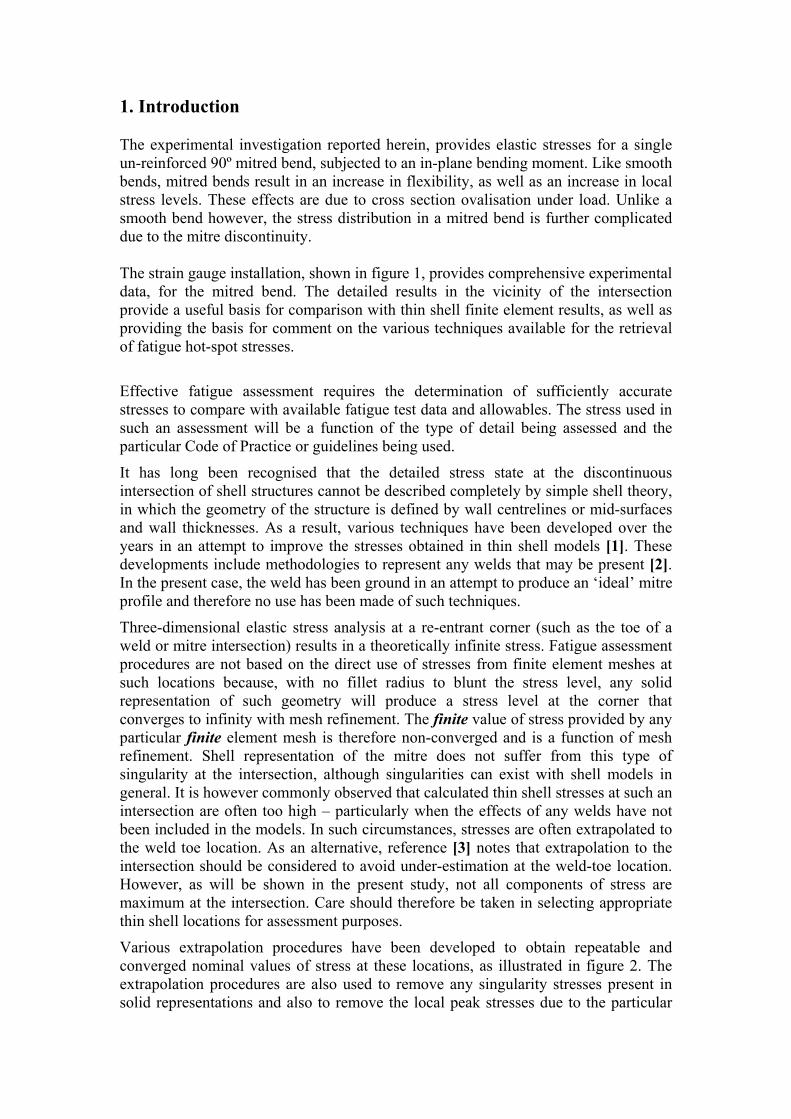
1 Introduction
The experimental investigation reported herein provides elastic stresses for a single
un-reinforced 90ordm mitred bend subjected to an in-plane bending moment Like smooth
bends mitred bends result in an increase in flexibility as well as an increase in local
stress levels These effects are due to cross section ovalisation under load Unlike a
smooth bend however the stress distribution in a mitred bend is further complicated
due to the mitre discontinuity
The strain gauge installation shown in figure 1 provides comprehensive experimental
data for the mitred bend The detailed results in the vicinity of the intersection
provide a useful basis for comparison with thin shell finite element results as well as
providing the basis for comment on the various techniques available for the retrieval
of fatigue hot-spot stresses
Effective fatigue assessment requires the determination of sufficiently accurate
stresses to compare with available fatigue test data and allowables The stress used in
such an assessment will be a function of the type of detail being assessed and the
particular Code of Practice or guidelines being used
It has long been recognised that the detailed stress state at the discontinuous
intersection of shell structures cannot be described completely by simple shell theory
in which the geometry of the structure is defined by wall centrelines or mid-surfaces
and wall thicknesses As a result various techniques have been developed over the
years in an attempt to improve the stresses obtained in thin shell models [1] These
developments include methodologies to represent any welds that may be present [2]
In the present case the weld has been ground in an attempt to produce an ideal mitre
profile and therefore no use has been made of such techniques
Three-dimensional elastic stress analysis at a re-entrant corner (such as the toe of a
weld or mitre intersection) results in a theoretically infinite stress Fatigue assessment
procedures are not based on the direct use of stresses from finite element meshes at
such locations because with no fillet radius to blunt the stress level any solid
representation of such geometry will produce a stress level at the corner that
converges to infinity with mesh refinement The finite value of stress provided by any
particular finite element mesh is therefore non-converged and is a function of mesh
refinement Shell representation of the mitre does not suffer from this type of
singularity at the intersection although singularities can exist with shell models in
general It is however commonly observed that calculated thin shell stresses at such an
intersection are often too high particularly when the effects of any welds have not
been included in the models In such circumstances stresses are often extrapolated to
the weld toe location As an alternative reference [3] notes that extrapolation to the
intersection should be considered to avoid under-estimation at the weld-toe location
However as will be shown in the present study not all components of stress are
maximum at the intersection Care should therefore be taken in selecting appropriate
thin shell locations for assessment purposes
Various extrapolation procedures have been developed to obtain repeatable and
converged nominal values of stress at these locations as illustrated in figure 2 The
extrapolation procedures are also used to remove any singularity stresses present in
solid representations and also to remove the local peak stresses due to the particular
weld geometry The reason for this is that fatigue allowables often already include
such local effects [3 4 5] These stresses are referred to as hot-spot stresses or
structural stresses Clearly these stresses are representative in nature and will not
necessarily exist at any point in the model or the real structure
Such extrapolation procedures have been used for many years In the late 1970s and
early 80s much work in this area was being carried out as part of the United
Kingdom Offshore Steels Research project [6] in the study of stresses in the joints of
tubular jacket structures In this case both experimental strain gauging and finite
elements were being used as a means of determining the toe hot-spot stresses
Comparisons with photoelastic models were also made Indeed the guidelines in
reference [3] provide different extrapolation methods for use with strain gauges and
finite element modelling The latter also includes different guidance for coarse and
fine meshes Fine mesh quadratic extrapolation (3 points) is recommended in special
cases where it is not possible to use the guidelines eg due to the closeness of two
welds The guidelines also introduce the notion of type a and b hot-spots with
different procedures for handling both Interestingly the guidance on meshing accepts
that non-converged results (coarse meshes) may be used as long as there are no other
severe discontinuities in the vicinity that the stress gradient is not high that standard
8-noded shell elements or 20-noded solids are used and that the stresses used are those
at the mid-side nodes It is argued that the error introduced by using relatively distant
extrapolation points is compensated by the slightly exaggerated midside node stresses
due to the influence of the singularity at the hot-spot corner node Such guidance is
clearly arising from the practicalities of modelling large fabricated structures where
representation of detail as small as welds is not practical However it is apparent that
converged results would provide a more consistent and logical basis for any
extrapolation method Ideally extrapolation methods should not be a function of the
shape function of elements used or the degree of mesh refinement No doubt such
guidance will evolve as available computing resources continue to increase The
converged results from the highly refined model of the mitre can possibly be used as
the basis for studying such developments and this is discussed further in section 43
2 Experiment
21 Test Rig
The test rig utilized a simple goal-post arrangement to subject the bend to a
transverse load via a hydraulic ram as shown in figure 3 This method of loading
subjected the horizontal leg of the bend to a linearly varying bending moment in
addition to a shearing action The vertical leg on the other hand was subjected to a
uniform bending moment in addition to a thrust action
In the experimental set-up shown in figure 3 the effect of the self-weight of the
horizontal leg was removed by use of a pulley arrangement
This general test configuration and data was also used as the basis for the finite
element model as shown in figure 4
22 Bend Specification and Manufacture
The test specimen shown in figure 3 was manufactured from carbon steel hot finished
seamless pipe [7] with nominal dimensions of 200mm diax 635mm thk The
measured bend angle of 892ordm resulted from inaccurate fit-up during the welding of
the mitre The intersection weld was ground flat
A thickness survey was carried out on the bend with an ultrasonic digital thickness
meter and values were measured at 79 locations on each leg The average thickness
was 653mm with a variation of plusmn45 A diameter survey across 28 diameters on
each leg was also carried out before and after welding The average OD was
1939mm with a variation of plusmn07 These values are well within the tolerances
permitted by reference [7] The thickness variation can have a significant effect on the
experimental stress values and this is discussed in section 4 It clearly would have
been possible to use pipe with a higher degree of tolerance on geometry However the
purpose of this paper was not to report a highly accurate comparison between finite
element analysis and experiment but to illustrate the real variations and practical
challenges that comparisons between idealized finite element models and as-built
structures entails
A total of eight tensile test specimens were manufactured from the pipe and tested in
accordance with BS EN 10002-1 [8] Two of the specimens had strain gauge pairs
attached to facilitate the determination of Poissons ratio The average values of E =
209 kNmm2 and ν = 028 were used in the finite element analyses
23 Instrumentation and Ancillary Equipment
Details of the electrical resistance strain gauges and the installation used in the
experiment are shown in table 1 All strain gauges were installed in accordance with
the guidelines given in references [9 10] with respect to surface preparation and
bonding After installation checks were made on resistance-to-earth and gauge
resistance for all strain gauges Gauges operated satisfactorily throughout the test A
total of 46 rosettes and 4 pairs were attached to the bend and these were connected
into the data logger in a 4-wire frac14 bridge configuration
To install the inside surface gauges the horizontal leg of the bend was cut
approximately 200mm from the intersection as indicated by the position of the weld
in figure 1 The actual length of pipe left had to be short enough to allow strain gauge
installation close to the mitre but not too short so as to avoid damage to the gauges
during the re-welding of the leg The inner surface gauges were covered with fire
protection cloth during re-welding to prevent weld spatter damage During the re-
welding operation the region of the intersection was continually cooled by a water
jacket and the temperature in the region of the gauges monitored with temperature
indication sticks
All gauges in the vicinity of the mitre intersection were in the form of rosettes to
enable the principal stresses and their directions to be determined The inner and outer
surface hoop distributions of gauges were located as close to the mitre intersection
as the gauge backing would allow The smallest rosettes had individual gauge lengths
of 038mm to enable the steep stress gradients to be accurately measured
The 90ordm and 60ordm positions were chosen for the longitudinal distributions of gauges
The 60ordm position is in the region of maximum stress as shown in the finite element
results In addition the 90ordm location possesses the characteristic of not having any
slope discontinuity between the shells
Strain gauge pairs located one metre from the intersection allowed an assessment of
loading symmetry to be made in addition to providing a membrane check The
rosettes at the -90ordm and -60ordm positions on the outer surface at the intersection also
provided a check on loading symmetry
All gauges used in the experiment were temperature compensated for steel The
energization current for all gauges was 83mA The gauges were scanned and
energized at the rate of 40 per second and no difficulty was experienced due to self-
heating of the gauges
The transverse load was applied to the bend by an Enerpac hydraulic ram of 30 kN
capacity as shown in figure 3 A needle valve was included in the hydraulic circuit
to permit accurate control of the loading The loading arrangement consisted of the
hydraulic ram a load cell a ball bearing resting in a spherical seat to take up any
misalignment of loading and also a bearing pad to distribute the load to the bend The
calibrated load cell used in the experiment provided a good strain output for the load
levels applied
Dial gauges with a resolution of 001 mm were used to measure both the bend and rig
deflection The latter was found to be negligible The dial gauges were located on a
frame built up from the floor End rotation of the bend was measured by a laser beam
which was deflected by a mirror attached to the end of the horizontal leg of the pipe
onto a measurement chart
24 Experimental Procedure
Some relevant details of the experimental procedure are outlined below
(i) The maximum load to be applied was established by monitoring all gauges at a low
load level The strain gauge exhibiting the highest strain level was established and this
value of strain was used to determine the load that would result in a strain of 1000 ȝİ for this particular gauge
(ii) The load was cycled 5 times from zero to maximum value
(iii) During the test checks were made on the symmetry of loading and adjustments
were made to the ram position as necessary
(iv) Loads were applied in 10 approximately equal increments up to the maximum
The loading was decreased from the maximum in 5 approximately equal increments
down to zero Dial gauge laser and strain gauge readings were taken at each
increment and all readings were linear with applied load
The experimental stress results were processed using strain gauge analysis software
The program analysed the various gauge configurations and also checked gauge
linearity For loading and unloading the maximum deviation from the combined
best-fit straight line was insignificant
3 Finite Element Model
Over the years numerous finite element analyses of mitred bends have been carried
out invariably using thin shell idealisations Sobieszczanski [11] recommended such
an approach over 35 years ago for this problem Possibly the earliest reference to the
actual use of finite elements for the study of a mitred bend is due to Edwards [12] in
1974 A comprehensive review of mitred bend publications from 1952 to date is
presented in reference [13] This review contains reference to 93 publications many
of which detail the development of analytical solutions by Kitching and others
However given the stated purpose of the present investigation comparisons with
such analytical results are not presented
The finite element model of the experimental specimen used in the present
investigation is shown in figure 4 The end of the vertical leg was assumed fully fixed
A half model was used as a result of symmetry The finite element results presented
were produced using shell elements as implemented in the Pro-Mechanica Applied
Structure system from Parametric Technology Inc The Applied Structure system uses
adaptive-p element technology which allows the user to specify a percentage
convergence for the analysis In the analyses reported here convergence was based
upon displacements strain energy and a global root-mean-squared stress measure
Convergence levels achieved were less than 1
The shortest element length in the vicinity of the intersection was 4mm However it
should be borne in mind that each p element can recover stresses over a 10 by 10
internal grid an can have a shape function up to a 9th
order polynomial The maximum
deflection of 73mm occurred at the end of the horizontal leg as expected and this
compared with an experimental value of 78mm The deformations have been
exaggerated in the scrap view in figure 4(a) to illustrate the ovalisation in the region
of the intersection Interestingly the thin shell finite element results show that the
maximum ovalisation does not occur at the intersection itself but a small distance
away (in this case 398mm) It should be noted however that the maximum radial
displacement is only 034mm and at the intersection it is only 028mm It was not
possible to measure such differences using the experimental equipment available to
verify this finite element result
4 Comparison of Results
41 Overall Deformations and Field Stresses
The end rotation of the horizontal leg is compared with the value obtained from the
finite element analysis in table 2 Also included in the table are the values derived for
a beam representation of the mitre in which there is no cross-sectional ovalisation
Reasonable agreement was obtained between experiment and finite element analysis
given the accuracy of the experimental measurement of rotation The experimental
results show slightly greater flexibility This may be due to the fact that the fully fixed
assumption used in the finite element model is not entirely realistic However it must
also be noted that an 005 degree difference in an end rotation of 03 degrees is also
on the limits of accuracy for the equipment used to measure rotation
The results obtained from the membrane check gauges on the vertical leg also
compared reasonably well with the values from beam bending theory and finite
element analysis The thickness survey carried out on the bend showed a -34
variation in thickness in the region of the intrados with only a -12 variation at the
extrados Stresses in the region of the check gauges are mainly membrane and will
therefore vary inversely with thickness This thickness variation does not entirely
explain the difference between the experimental and finite element results however
Another contribution to the difference in results is due to the fact that in the finite
element analysis the load was applied normal to the horizontal leg which in fact
was not quite horizontal due to the bend angle of 892 degrees This small angle
makes a difference of approximately 05Nmm2 at the check gauge positions
compared to a vertical load due to the resulting variation in bending moment Any
lack of perpendicularity in the test rig set-up of a similar magnitude could also have
resulted in similar variations A slight lack of symmetry was also evident in the
experimental results from the check gauges which is perhaps indicative of a lack of
precision in the test geometry
42 Stresses at Intersection
The maximum finite element stresses occur at the intersection and these values are
presented in table 3
The stress direction shown in table 3 is relative to the mitre intersection The stress
divisor used in calculating the Stress Concentration Factor was the nominal bending
stress in a straight pipe of the same dimensions and with a moment M = F x Leg
length ie trm 2πM
For an in-plane moment tending to close the bend the largest stress is compressive
As show in table 3 two almost identical values occur at different locations one on
the outer surface at 51 degrees and the other on the inner surface at 75 degrees The
former is in a direction normal to the intersection and the latter along the intersection
For a load of the same magnitude opening the bend all values of deflection rotation
and stress would have the same magnitude but different signs (for small displacement
linear elastic analysis)
Although not shown herein it was observed that the directions of the principal
stresses were perpendicular and parallel to the intersection (as expected from
symmetry) The longitudinal distributions (experimental and FEA) show the angle of
the principal stresses returning to the axial and circumferential directions with
increase in distance from the intersection It was also apparent that the unsymmetrical
nature of the transverse load was insignificant in regions close to the mitre also as
expected The applied bending moment is obviously the same for each leg at the mitre
intersection This symmetry is confirmed by the fringe pattern shown in figure 4(b)
While the finite element results are obviously symmetrical about the 0ordm180ordm positions
due to the applied constraints the experimental results from the check gauges showed
some slight lack of symmetry This lack of symmetry became more evident at higher
load levels and proved difficult to control by adjusting the loading ram However this
slight lack of symmetry is not sufficient to invalidate comparisons with FEA as
illustrated by the following comparisons
In figures 5 and 6 the outer surface principal stress distributions at 4mm from the
intersection show good agreement in both form and magnitude The inner surface
experimental stresses also show reasonable agreement with the finite element
analysis in spite of the somewhat larger gauge sizes used on the inner surface
Preparation on the inner surface for the purposes of gauge installation was also
affected slightly due to small surface imperfections very close to the intersection
Clearly the significance of any surface imperfections increases with the use of small
gauge lengths
The agreement for principal stress decay shown in figures 7 and 8 is reasonable with
the trends in distribution comparing particularly favorably The comparison at the 60
degree location is better The magnitudes of the stresses at this location are greater
and the decay length is shorter It is a common observation that experimental decay
curves appear displaced from thin shell finite element distributions when modeling
this type of intersection [1] However such displacement is normally of the order of
half a shell thickness at most In the case of the mitre the theoretical shell
displacement δ will vary depending whether the inside(+) or outside(-) surface is
being considered according to the relationship θψcos
2tan
2 ⎟⎟⎠
⎞⎜⎜⎝
⎛⎟⎠⎞
⎜⎝⎛plusmn
t where t is the
shell thickness ψ is the mitre angle and θ is the angular location shown in figures
1 and 4 Clearly such a displacement of distributions does not explain the
differences between experiment and finite element analysis in this case The survey
of wall thickness shows that the values at the 90 degree position in the vicinity of the
mitre are 44 above average A check on the proportions of bending and membrane
stress at the 90 degree position approximately 54mm away from the mitre
intersection (where the differences are largest in figure 7) showed that the ratios are
25 and 84 for the two principal stresses Given that the bending stresses which
therefore dominate in this region vary inversely with thickness squared it is apparent
that this thickness increase would result in a proportionately larger reduction in stress
magnitude This in itself would not explain the larger differences in figure 7
However it is also possible that the thickening in the pipe wall at this location could
lead to a reduction in ovalisation which would in turn reduce the magnitude of the
experimental results further The fact that the thin shell finite element results are
higher than the experimental values in general is obviously conservative from a
design viewpoint In the case of the extrapolated hot-spot stresses the thin-shell
over-estimate is of the order of 7 12 as shown in table 4
43 Hot-Spot Stresses
Although the finite element extrapolation guidance in reference [3] is not intended for
use with the highly refined mesh used for the mitre it is informative to compare any
differences arising from the various methods when applied to a converged finite
element model Extrapolated hot-spot stresses obtained from the finite element and
experimental results are compared with the raw finite element results at the
intersection in table 4 Both linear (2-point) and quadratic (3-point) extrapolation is
used
For extrapolation purposes reference [14] recommends a strain gauge length of less
than 02t (127mm in this case) As indicated in table 1 all gauges used for the mitre
in the vicinity of the intersection satisfy this requirement However despite the 120
degree rosettes having an individual gauge length of only 038mm the distance from
the intersection to the centre of the closest rosette was 4mm rather than the
recommended 04t (254mm in this case) In the present investigation therefore
quadratic extrapolation was used for the experimental results as values were available
at 4813mm which is almost identical to the 4812mm recommendations of
reference [3]
The values in table 4 appear encouraging However when the logarithmic nature of
typical S-N curves is considered [4] along with the slope of the curve then such
variations between finite elements and experiment may still result in significant
differences in life predictions It is not perhaps surprising that both linear and
quadratic extrapolation provide similar results to the actual intersection stresses given
that the mesh is highly refined and converged to within 1 However the reversal in
stress close to the mitre as shown in figure 7 is not untypical for refined shell finite
element models of intersection problems in general and clearly care would be required
in such circumstances with linear extrapolation in particular to ensure that the correct
trend is picked up Bearing in mind that the present experiment used rosettes with
individual gauge lengths of approximately a third of a millimetre it would not have
been possible to use more gauges in an attempt to refine the experimental
distributions Not surprisingly quadratic extrapolation provides more accurate results
in this case As expected the thin shell results at the intersection represent a
conservative position when compared with experiment However given the form of
the decay distributions shown in figures 7 and 8 it is apparent that some stresses at
the intersection may in fact be smaller when compared with results at the weld toe
location Given that the fatigue assessment procedures in some Codes [4 5] requires
stresses to be used in particular directions which may not be the absolute maximum
it is important that both weld toe and intersection locations are considered
The thin shell results at the intersection are very close to those obtained by
extrapolation of the finite element results to the intersection This is to be expected
given the highly refined nature of the mesh
The thin shell finite element results are in fact consistent in nature with through
thickness linearization techniques illustrated in figure 2 for the weld toe position
Through thickness linearization techniques are used with 3-D solid models (and 2-D
solid of revolution) to remove the peak stress component Through-thickness
linearization is an effective alternative to surface extrapolation methods and has the
advantage of simplicity and is consistent with the use of linearization for other
purposes in the Code design and assessment of vessels It also has the advantage of
being insensitive to the stress reversal trends mentioned previously The use of thin
shell elements obviously means that such linearization is not required Dong [15] has
long been a proponent of a through-thickness linearization approach
5 Conclusions
It is likely that better comparisons between experiment and finite element analysis
could have been obtained by use of a more accurate test specimen with tighter
tolerances on dimensions and manufacture The use of 3D solid elements would also
have served to eliminate the approximations inherent in shell solutions However this
relatively simple fabricated steel structure has highlighted many of the challenges
faced in conducting effective experimental investigations and finite element studies
involving welded discontinuous intersections of shells Even with extensively
instrumented specimens using some of the smallest gauge lengths available it is not
always possible to pick up the local stress variations apparent in thin shell finite
element models For example the experimental results do not exhibit the localized
stress reversal shown in figure 7
Such areas are susceptible to fatigue failure and the recovery of hot-spot stresses is
invariably dependent on accurate stress fields in the vicinity of the intersection In this
respect the raw finite element and experimental values for maximum stress at the
intersection are in reasonable agreement In addition for the highly refined mesh
used there is little difference between linear and quadratic extrapolation techniques
All extrapolation techniques when used with the finite element results produce
almost identical results to the raw thin shell finite element values at the intersection
The extrapolated experimental hot-spot stress values are however 7-12 lower than
the raw finite element results at the intersection This level of variation should be
borne in mind when assessing the accuracy of any fatigue analysis as this can lead to
significant variations in life prediction using the logarithmic S-N data
The very local reversal in trend of the stress decay variation which occurs in many
shell intersection problems can clearly cause errors with surface extrapolation
techniques It is worth noting that the through-thickness linearization approach to
obtaining hot spot or structural stress using 3D solid elements is not susceptible to
this problem These typical reversals in trend may also mean that the intersection
stress value may not be the largest as is often assumed Some pressure vessel codes
require stresses in particular directions to be used which may be smaller in magnitude
than the absolute maximum value of principal stress These stresses for cracks
running in particular directions may also have a lower allowable than the absolute
maximum principal stress It is important therefore that such trends in decay
distributions are considered for thin shell models and that appropriate worst-case
scenarios are postulated A finite element investigation using 3D solid elements could
help to establish whether such a localized reversal in trend is a function of the thin
shell idealization Such a model would also be useful to study the location of the
maximum position of ovalisation A 3D solid representation would off course bring
the additional problem of introducing a singularity
Acknowledgements
The advice and assistance of my former colleagues David Cloney and George Findlay
is gratefully acknowledged
References
1 Wood J Observations on Shell Intersections 4th
World Congress on Finite
Element Methods Interlaken September 1984
2 Wood J Procedural Benchmarks for Common Fabrication Details in PlateShell
Structures NAFEMS Publication ISBN 1-874-376-02-6 2005
3 Niemi E et al Fatigue Analysis of Welded Components Design Guide to the
Structural Hot-spot Stress Approach (IIW-1430-00) Woodhead Publishing Ltd
ISBN-13 978-1-84569-124-0 2006
4 BSI Specification for Unfired Fusion Welded Pressure Vessels PD5500 2000
5 BSI Eurocode 3 Design of Steel Structures BS EN 1993-1-9 2005
6 Peckover RS et al United Kingdom Offshore Steels Research Project Phase 1
Final Report OTH 88 282 UK Department of Energy 1985
7 BSI Specification for Carbon Steel Pipes and Tubes with Specified Room
Temperature Properties for Pressure Purposes BS3601 1987
8 BSI Tensile Testing of Metallic Materials Method of Test at Ambient
Temperature BS EN 10002-1 2001
9 Pople J BSSM Strain Measurement Reference Book British Society of Strain
Measurement 1979
10 Vishay Strain Gauge Installations with M-Bond 200 Adhesive Instruction
Bulletin B-127 Micro Measurement
11 Sobieszczanski J Strength of a Pipe Mitred Bend J of Engineering for Industry
Nov 1970
12 Edwards G Cylindrical Shell Hybrid Finite Elements PhD Thesis University of
Nottingham 1974
13 Wood J A Review of the Literature for the Structural Assessment of Mitred
Bends Submitted for Publication to the Int J of Pressure Vessels and Piping
Oct 2006
14 Hobbacher A Recommendations for Fatigue Design of Welded Joints and
Components IIW Report XIII-1539-96 Update June 2002
15 Dong P A Structural Stress Definition and Numerical Implementation for
Fatigue Analysis of Welded Joints Int J Fatigue 23 pp865-876 2001
LIST OF CAPTIONS
Table 1 Details of Strain Gauges
Table 2 Comparison of Overall Deformation and Field Stresses
Table 3 Maximum Finite Element Stresses at Intersection
Table 4 Maximum Finite Element Stresses at Intersection
Figure 1 Mitred Bend Showing Strain Gauges
Figure 2 Various Hot Spot Stress Techniques for Intersections and Welds
Figure 3 Test Arrangement for Mitred Bend
Figure 4 Adaptive P-method Finite Element Model with von Mises Stress
Superimposed on Deformed Shape
Figure 5 Maximum Principal Stress Variation Near Mitre Intersection
Figure 6 Minimum Principal Stress Variation Near Mitre Intersection
Figure 7 Principal Stress Decay at 90 Degree Location
Figure 8 Principal Stress Decay at 60 Degree Location
GAUGE NUMBER
amp
ALIGNMENT
GAUGE TYPE
amp
INDIVIDUAL
GAUGE LENGTH
(mm)
INSTALLATION SURFACE
amp
MANUFACTURERS
SPECIFICATION
DISTANCE FROM MITRE
INTERSECTION TO CENTRE OF
CONFIGURATION (mm)
amp
ANGULAR POSITION (deg)
1 to14 Normal to intersection 120ordm Rosette 038mm Outer MM EA-06-015RC-120 4 140125-75 in 5 inc 40 10
35 amp 36 Normal to intersection 120ordm Rosette 038mm Outer MM EA-06-015RC-120 4 -90 -60 (Check gauges)
15 to 18 Middle gauge axial 120deg Rosette 038mm Outer MM EA-06-015RC-120 8 13 205 285 90
19 to 25 Middle gauge axial 90deg Rosette 137mm Outer MM EA-06-062RB-120 42 625 84 105 126 1465 457 90
26 to 30 Middle gauge axial 120ordmRosette 038mm Outer MM EA-06-015RC-120 8 13 19 25 31 60
31(1-5) Strip Middle gauge axial 120deg Rosette 12mm Outer HBM 4120 KY31 375 415 455 495 535 60
32 to 34 Middle gauge axial 90deg Rosette 137mm Outer MM EA-06-062RB-120 80 146 457 60
37 Axial amp hoop 90deg Pair 157mm Outer MM EA-06-062TT-120 905 0
38 amp 40 Axial amp hoop 90deg Pair 157mm Outer MM EA-06-062TT-120 1000 90 -90
39 Axial amp hoop 90deg Pair 157mm Outer MM EA-06-062TT-120 1095 180
41 to 46 Middle gauge axial 90deg Rosettes 2mm Inner Showa N31-FA-2 4 0 45 90 0 -90 -45
Note Intrados = 0 degrees and Extrados = 180 degrees
Table 1 Details of strain gauges
Rotation
of
Horizontal Leg
(deg)
Vertical Deflection
End of Horizontal
Leg
(mm)
Maximum Principal
Stress Extrados
1000mm from mitre
(Nmm2)
Maximum Principal
Stress Intrados
1000mm from mitre
(Nmm2)
Experiment 035 78 283 -327
Beam Theory
(no ovalisation)
016 37 275 -298
FEA 030 73 284 -302
Table 2 Comparison of Overall Deformation and Field Stresses
Maximum
Principal
Stress
(Nmm2)
Angular
Position
θ (deg)
Stress
Direction
Maximum
SCF
Minimum
Principal
Stress
(Nmm2)
Angular
Position
θ (deg)
Stress
Direction
Maximum
SCF
Outer
Surface 1517 840 Normal 52 -2857 506 Normal -98
Inner
Surface 2111 435 Normal 72 -2858 745 Hoop -98
Table 3 Maximum Finite Element Stresses at Intersection
FE Thin Shell
Intersection
(Nmm2)
FE Thin Shell
Extrapolated
04t10t
(Nmm2) [3]
FE Thin Shell
Extrapolated
4812 mm
(Nmm2) [3]
Experimental
Extrapolated
4813 mm
(Nmm2)
Outer Surface
90 degrees 1233 1263 1250 1147
Inner Surface
90 degrees -941 -959 -942 -
Outer Surface
60 degrees -2693 -2635 -2668 -2392
Inner Surface
60 degrees 1559 1513 1542 -
Table 4 Maximum Finite Element Stresses at Intersection
Figure 1 Mitred Bend Showing Strain Gauges
Figure 2 Various Hot Spot Stress Techniques for Intersections and Welds
Figure 3 Test Arrangement for Mitred Bend
Figure 4 Adaptive P-method Finite Element Model with von Mises Stress
Superimposed on Deformed Shape
Maximum Principal Stress Variation at 4mm from Mitre Intersection
-150
-100
-50
0
50
100
150
200
0 90 180
Angular Position (degrees)
Str
es
s (
Ns
qm
m)
Finite Element Outer Surface
Finite Element Inner Surface
Experimental Outer Surface
Experimental Inner Surface
Figure 5 Maximum Principal Stress Variation Near Mitre Intersection
Minimum Principal Stress Variation at 4mm from Mitre Intersection
-300
-250
-200
-150
-100
-50
0
50
100
150
0 90 180
Angular Position (degrees)
Str
es
s (
Ns
qm
m)
Finite Element Outer Surface
Finite Element Inner Surface
Experimental Outer Surface
Experimental Inner Surface
Figure 6 Minimum Principal Stress Variation Near Mitre Intersection
Principal Stress Decay at 90 Degrees
-200
-150
-100
-50
0
50
100
150
0 50 100 150 200 250 300 350 400 450 500
Distance From Mitre (mm)
Str
es
s (
Ns
qm
m)
Finite Element Maximum Principal Outer
Finite Element Maximum Principal Inner
Experimental Maximum Principal Outer
Experimental Minimum Principal Outer
Finite Element Minimum Principal Outer
Finite Element Minimum Principal Inner
Figure 7 Principal Stress Decay at 90 Degree Location
Principal Stress Decay at 60 Degrees
-300
-250
-200
-150
-100
-50
0
50
100
150
200
0 50 100 150 200 250 300 350 400 450 500
Distance From Mitre (mm)
Str
es
s (
Ns
qm
m)
Finite Element Maximum Principal Outer
Finite Element Maximum Principal Inner
Experimental Maximum Principal Outer
Experimental Minimum Principal Outer
Finite Element Minimum Principal Outer
Finite Element Minimum Principal Inner
Figure 8 Principal Stress Decay at 60 Degree Location
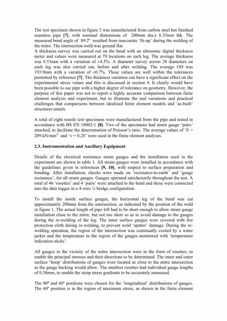
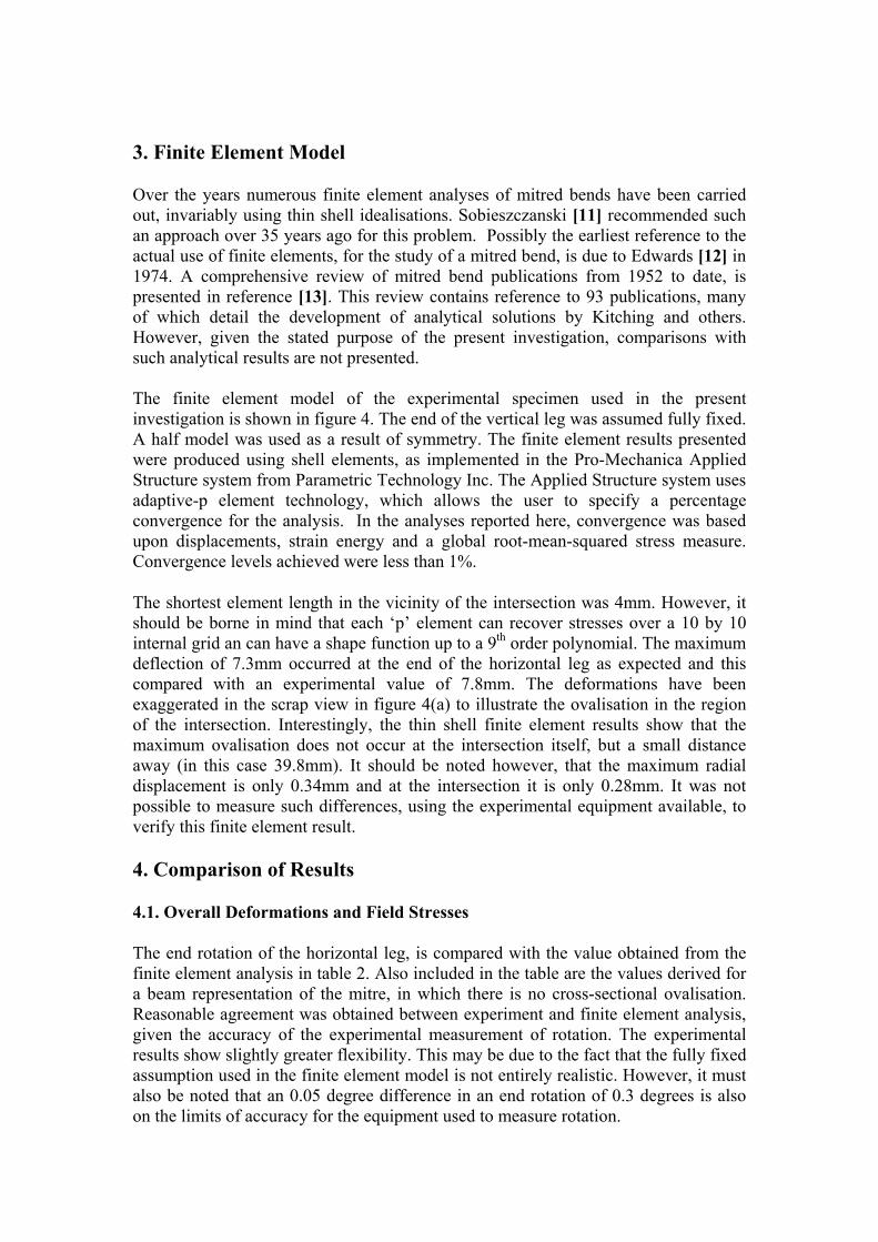
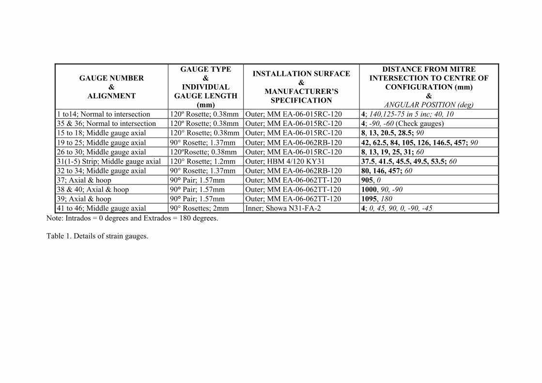
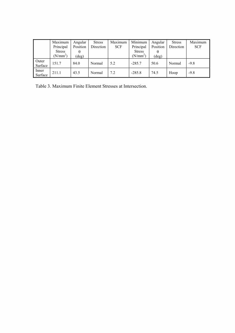
Maximum
Principal
Stress
(Nmm2)
Angular
Position
θ (deg)
Stress
Direction
Maximum
SCF
Minimum
Principal
Stress
(Nmm2)
Angular
Position
θ (deg)
Stress
Direction
Maximum
SCF
Outer
Surface 1517 840 Normal 52 -2857 506 Normal -98
Inner
Surface 2111 435 Normal 72 -2858 745 Hoop -98
Table 3 Maximum Finite Element Stresses at Intersection
FE Thin Shell
Intersection
(Nmm2)
FE Thin Shell
Extrapolated
04t10t
(Nmm2) [3]
FE Thin Shell
Extrapolated
4812 mm
(Nmm2) [3]
Experimental
Extrapolated
4813 mm
(Nmm2)
Outer Surface
90 degrees 1233 1263 1250 1147
Inner Surface
90 degrees -941 -959 -942 -
Outer Surface
60 degrees -2693 -2635 -2668 -2392
Inner Surface
60 degrees 1559 1513 1542 -
Table 4 Maximum Finite Element Stresses at Intersection
Figure 1 Mitred Bend Showing Strain Gauges
Figure 2 Various Hot Spot Stress Techniques for Intersections and Welds
Figure 3 Test Arrangement for Mitred Bend
Figure 4 Adaptive P-method Finite Element Model with von Mises Stress
Superimposed on Deformed Shape
Maximum Principal Stress Variation at 4mm from Mitre Intersection
-150
-100
-50
0
50
100
150
200
0 90 180
Angular Position (degrees)
Str
es
s (
Ns
qm
m)
Finite Element Outer Surface
Finite Element Inner Surface
Experimental Outer Surface
Experimental Inner Surface
Figure 5 Maximum Principal Stress Variation Near Mitre Intersection
Minimum Principal Stress Variation at 4mm from Mitre Intersection
-300
-250
-200
-150
-100
-50
0
50
100
150
0 90 180
Angular Position (degrees)
Str
es
s (
Ns
qm
m)
Finite Element Outer Surface
Finite Element Inner Surface
Experimental Outer Surface
Experimental Inner Surface
Figure 6 Minimum Principal Stress Variation Near Mitre Intersection
Principal Stress Decay at 90 Degrees
-200
-150
-100
-50
0
50
100
150
0 50 100 150 200 250 300 350 400 450 500
Distance From Mitre (mm)
Str
es
s (
Ns
qm
m)
Finite Element Maximum Principal Outer
Finite Element Maximum Principal Inner
Experimental Maximum Principal Outer
Experimental Minimum Principal Outer
Finite Element Minimum Principal Outer
Finite Element Minimum Principal Inner
Figure 7 Principal Stress Decay at 90 Degree Location
Principal Stress Decay at 60 Degrees
-300
-250
-200
-150
-100
-50
0
50
100
150
200
0 50 100 150 200 250 300 350 400 450 500
Distance From Mitre (mm)
Str
es
s (
Ns
qm
m)
Finite Element Maximum Principal Outer
Finite Element Maximum Principal Inner
Experimental Maximum Principal Outer
Experimental Minimum Principal Outer
Finite Element Minimum Principal Outer
Finite Element Minimum Principal Inner
Figure 8 Principal Stress Decay at 60 Degree Location

FE Thin Shell
Intersection
(Nmm2)
FE Thin Shell
Extrapolated
04t10t
(Nmm2) [3]
FE Thin Shell
Extrapolated
4812 mm
(Nmm2) [3]
Experimental
Extrapolated
4813 mm
(Nmm2)
Outer Surface
90 degrees 1233 1263 1250 1147
Inner Surface
90 degrees -941 -959 -942 -
Outer Surface
60 degrees -2693 -2635 -2668 -2392
Inner Surface
60 degrees 1559 1513 1542 -
Table 4 Maximum Finite Element Stresses at Intersection
Figure 1 Mitred Bend Showing Strain Gauges
Figure 2 Various Hot Spot Stress Techniques for Intersections and Welds
Figure 3 Test Arrangement for Mitred Bend
Figure 4 Adaptive P-method Finite Element Model with von Mises Stress
Superimposed on Deformed Shape
Maximum Principal Stress Variation at 4mm from Mitre Intersection
-150
-100
-50
0
50
100
150
200
0 90 180
Angular Position (degrees)
Str
es
s (
Ns
qm
m)
Finite Element Outer Surface
Finite Element Inner Surface
Experimental Outer Surface
Experimental Inner Surface
Figure 5 Maximum Principal Stress Variation Near Mitre Intersection
Minimum Principal Stress Variation at 4mm from Mitre Intersection
-300
-250
-200
-150
-100
-50
0
50
100
150
0 90 180
Angular Position (degrees)
Str
es
s (
Ns
qm
m)
Finite Element Outer Surface
Finite Element Inner Surface
Experimental Outer Surface
Experimental Inner Surface
Figure 6 Minimum Principal Stress Variation Near Mitre Intersection
Principal Stress Decay at 90 Degrees
-200
-150
-100
-50
0
50
100
150
0 50 100 150 200 250 300 350 400 450 500
Distance From Mitre (mm)
Str
es
s (
Ns
qm
m)
Finite Element Maximum Principal Outer
Finite Element Maximum Principal Inner
Experimental Maximum Principal Outer
Experimental Minimum Principal Outer
Finite Element Minimum Principal Outer
Finite Element Minimum Principal Inner
Figure 7 Principal Stress Decay at 90 Degree Location
Principal Stress Decay at 60 Degrees
-300
-250
-200
-150
-100
-50
0
50
100
150
200
0 50 100 150 200 250 300 350 400 450 500
Distance From Mitre (mm)
Str
es
s (
Ns
qm
m)
Finite Element Maximum Principal Outer
Finite Element Maximum Principal Inner
Experimental Maximum Principal Outer
Experimental Minimum Principal Outer
Finite Element Minimum Principal Outer
Finite Element Minimum Principal Inner
Figure 8 Principal Stress Decay at 60 Degree Location
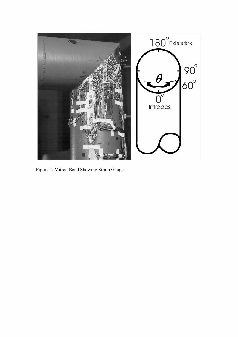
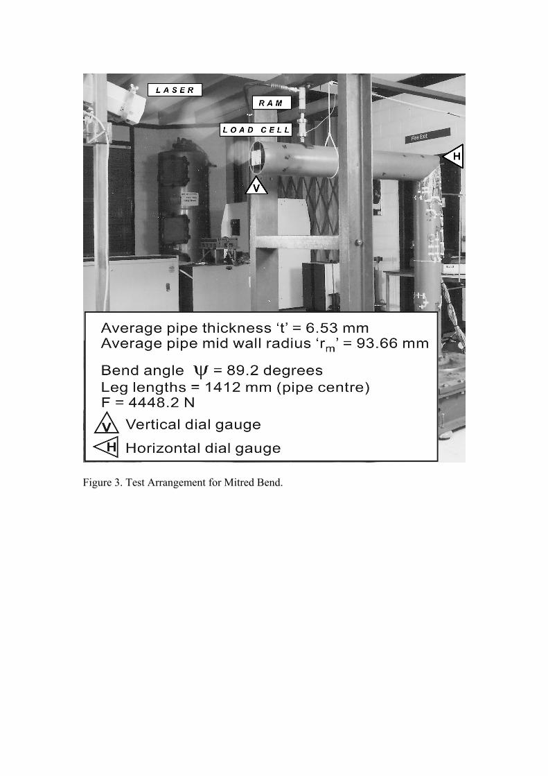
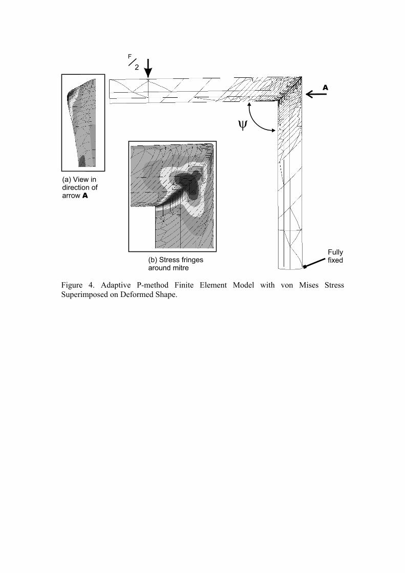
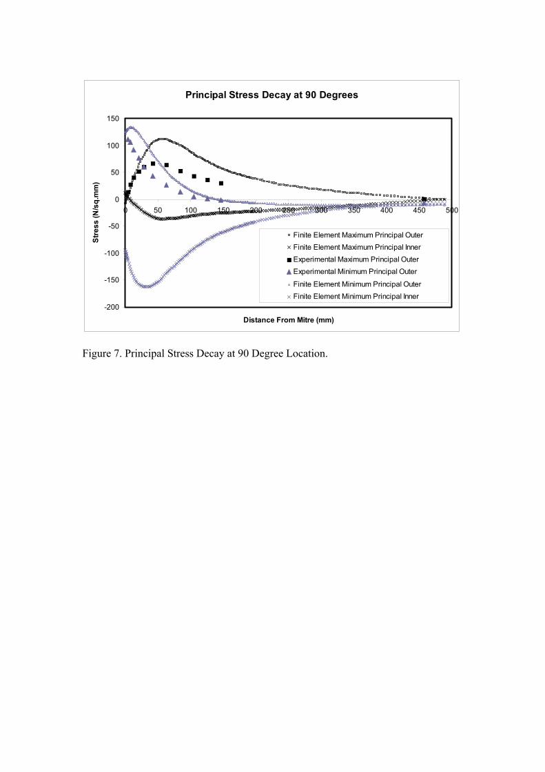