Stress testing in the Debt Sustainability Framework (DSF...
28
KNOWLEDGE BRIEF ECONOMIC POLICY AND DEBT DEPARTMENT (PRMED) • WORLD BANK Stress testing in the Debt Sustainability Framework (DSF) for Low-Income Countries François Painchaud 1 and Tihomir (Tish) Stučka 2 May, 2011 Summary: This technical note describes in detail the propagation of standardized stress tests in the LIC DSA template using an analytical and graphical approach. It is intended to aid technical staff in low income countries as well as country teams at the IMF and WB by providing the intuition as well as mechanics of stress testing. This should enhance the understanding of the shocks in the DSF and help improve the conduct of debt sustainability exercises in low income countries. 1 The views expressed herein are those of the authors and should not be attributed to the IMF, its Executive Board, or its management. 2 The views expressed herein are those of the authors and should not be attributed to the World Bank, its Executive Board, or its management.
Transcript of Stress testing in the Debt Sustainability Framework (DSF...
KNOWLEDGE BRIEF
ECONOMIC POLICY AND DEBT DEPARTMENT (PRMED) • WORLD BANK
Stress testing in the Debt Sustainability Framework (DSF) for
Low-Income Countries
François Painchaud1 and Tihomir (Tish) Stučka2
May, 2011
Summary: This technical note describes in detail the propagation of standardized stress
tests in the LIC DSA template using an analytical and graphical approach. It is intended
to aid technical staff in low income countries as well as country teams at the IMF and
WB by providing the intuition as well as mechanics of stress testing. This should enhance
the understanding of the shocks in the DSF and help improve the conduct of debt
sustainability exercises in low income countries.
1 The views expressed herein are those of the authors and should not be attributed to the IMF, its Executive
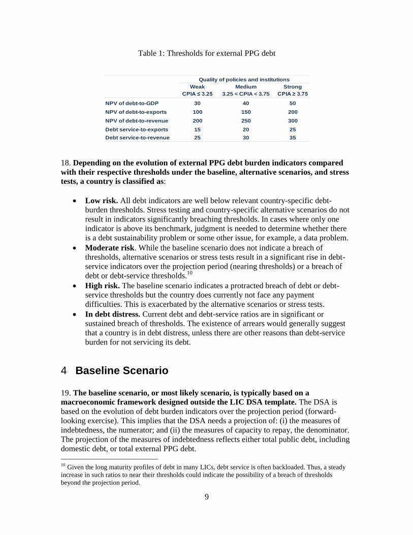
Board, or its management. 2 The views expressed herein are those of the authors and should not be attributed to the World Bank, its
Executive Board, or its management.

2
3
Table of Contents
1 INTRODUCTION .............................................................................................................................. 5
2 DEBT BURDEN INDICATORS ............................................................................................................ 6
3 DEBT SUSTAINABILITY ..................................................................................................................... 8
4 BASELINE SCENARIO ....................................................................................................................... 9
5 STANDARDIZED STRESS TESTS....................................................................................................... 11
5.1 SHOCK TO REAL GDP GROWTH (PDSA AND EDSA) ................................................................................... 15 5.2 EXCHANGE RATE DEPRECIATION (PDSA AND EDSA) .................................................................................. 16 5.3 SHOCK TO THE PRIMARY BALANCE (PDSA) ............................................................................................... 17 5.4 SHOCK TO THE PRIMARY BALANCE AND REAL GDP GROWTH (PDSA) ............................................................. 18 5.5 SHOCK TO OTHER DEBT CREATING FLOWS (PDSA) ..................................................................................... 19 5.6 HISTORICAL SCENARIO: SHOCK TO NON-INTEREST EXTERNAL CURRENT ACCOUNT, NET FDI, REAL GDP GROWTH, AND
GDP DEFLATOR IN US DOLLAR TERMS (EDSA) ................................................................................................... 20 5.7 SHOCK TO TERMS OF FOREIGN FINANCING (EDSA) .................................................................................... 22 5.8 SHOCK TO EXPORTS (EDSA) .................................................................................................................. 22 5.9 SHOCK TO DOMESTIC GDP DEFLATOR IN DOLLAR TERMS (EDSA) ................................................................. 24 5.10 SHOCK TO NON-DEBT CREATING FLOWS (EDSA) .................................................................................. 24 5.11 SHOCK TO REAL GDP, EXPORTS, GDP DEFLATOR, AND NON-DEBT CREATING FLOWS (ESDA) ........................ 25
6 CONCLUSION ................................................................................................................................ 27
7 REFERENCES .................................................................................................................................. 28

4
5
1 Introduction
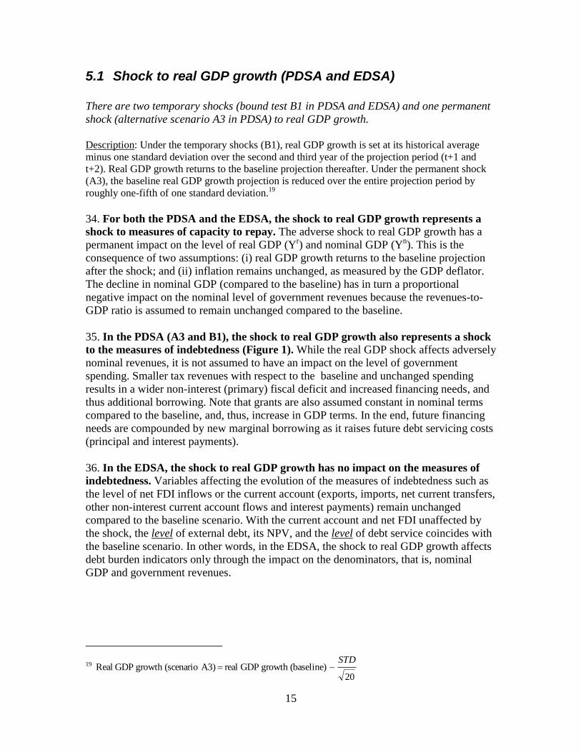
1. The objective of the joint Fund-Bank debt sustainability framework (DSF) for
low-income countries (LICs) is to support LICs’ efforts to achieve their
development goals without creating future debt problems.3 The DSF is built on three
pillars: (i) a standardized forward-looking analysis of debt and debt-service dynamics
under a baseline scenario, alternative scenarios, and standardized stress test scenarios; (ii)
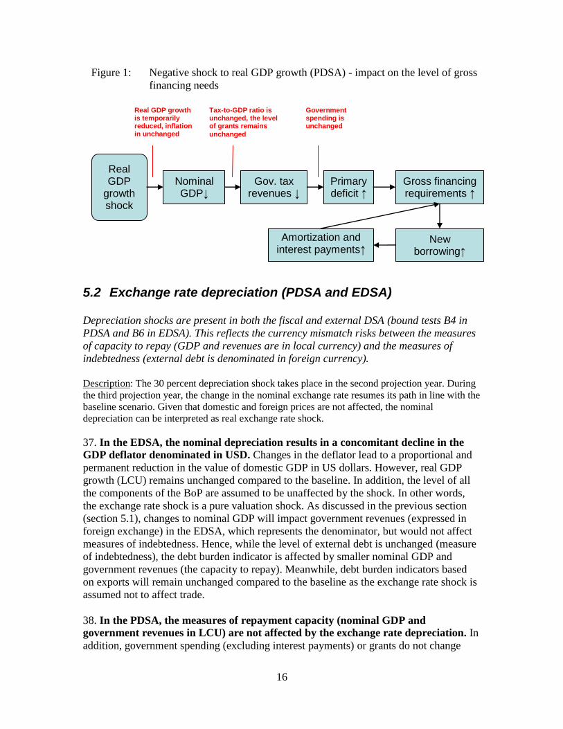
a debt sustainability assessment based on indicative country-specific debt-burden
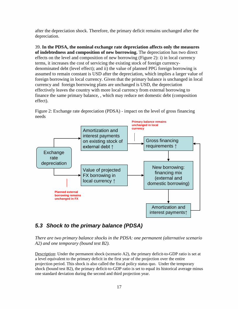
thresholds that depend on the quality of policies and institutions in the country; and (iii)
recommendations on a borrowing (and lending) strategy to limit the risk of debt distress,
while maximizing the resource envelope to achieve the Millennium Development Goals
(MDGs). The DSF is operationalized through the joint Bank-Fund debt sustainability
analysis (DSA) which is epitomized by the LIC DSA template.
2. The LIC DSA template combines the assessment of external and public debt
sustainability in one file. Public DSA covers external and domestic public and publicly
guaranteed (PPG) debt4, whereas the external DSA covers the country’s overall financing
flows with the rest of the world – external PPG and private debt.
3. To adequately inform borrowing and lending decisions, DSAs need to be based
on realistic macroeconomic baseline scenarios. The principal mechanism for
promoting realism in DSAs is to scrutinize baseline projections by (i) subjecting them to
reality checks and (ii) making use of precautionary features of the DSF. The reality
checks and precautionary features are intended to provide safeguards against excessive
borrowing and a return to debt distress, without constraining justified optimism about the
effective use of external resources to promote growth, reduce poverty, and achieve the
country’s development goals.
4. The LIC DSA template contains 16 standardized shocks. The standardized shocks
are deterministic with simplified feedback effects to ensure cross-country comparability.
To understand the underlying dynamics of the DSF, it is imperative to comprehend the
propagation of individual shocks through the economy.
3 The LIC DSF was formally introduced in 2005. See ―Operational Framework for Debt Sustainability
Assessments in Low-Income Countries—Further Considerations‖ and ―Debt Sustainability in Low-Income
Countries―Further Considerations on an Operational Framework and Policy Implications‖.
4 PPG debt comprises: (i) debt of the public sector, defined as central, regional and local governments,
central bank, and public enterprises—the latter subsumes all enterprises that the government controls, such
as by owning more than half of the voting shares—and (ii) private sector debt guaranteed by the public
sector. Excluding an SOE’s external debt from the external DSAs can be considered, if the company can
borrow externally without a public guarantee and its operations pose a limited fiscal risk. For more
information, please see ―Staff Guidance Note on the Application of the Joint Bank-Fund Debt
Sustainability Framework for Low-Income Countries‖.

6
5. The purpose of the paper is to provide a description of the stress tests. It
combines an analytical and graphical approach to describing the transmission
mechanisms of the shock in the LIC DSA template.
6. The paper proceeds as follows. Section 2 describes the concept of debt burden
indicators, which are central to the debt sustainability assessment. Section 3 discusses the
interpretation of debt burden outcomes in terms of risks of debt distress. In Section 4, the
baseline scenario is discussed, which is followed in Section 5 by a detailed description of
the stress tests. Section 6 concludes.
2 Debt burden indicators
8. Debt sustainability is assessed by undertaking a forward-looking analysis of the
evolution of debt burden indicators under a baseline scenario, alternative scenarios,
and standardized stress test scenarios. Debt burden indicators compare a measure of
indebtedness to a measure of capacity to repay:
repay ocapacity t of Measure
ssIndebtedne of Measure indicator burden Debt (1)
9. Different measures of indebtedness are used to identify solvency and liquidity
risks. Liquidity problems arise when a country has short term difficulties meeting its
financial obligations as they come due although its ability to pay is not affected under
normal circumstances. Solvency problems, on the other hand, arise when a country’s
repayment difficulties are permanent or protracted. Put differently, insolvency is
associated with policies that lead to ever-increasing debt levels in relative terms, which
necessitate a shift in policies such as an increase in taxes, cuts in spending, recourse to
monetization, or even repudiation.
10. Indicators based on debt stocks are used to identify possible solvency problems.
For LICs, a debt stock measure based on the present value (PV) of debt is more
informative than the nominal stock of debt5, reflecting the typical concessionality of
loans contracted by LICs (equation 2). Concessional loans are characterized by below-
market interest rates, a grace period, and a long maturity period. Clearly, the debt burden
5 The present value of debt is the sum of all future debt service payments (principal and interest) discounted
using an appropriate discount rate. The PV represents the amount of money to be invested today (earning
the discount rate) required to repay all the financial obligations stemming from the existing stock of debt.
Given that the calculations assume no capital losses, the discount rate to be used in PV calculations should
be the risk-free interest rate (r in equation 2). The discount rate in the LIC template is related to the six-
month average of the U.S. dollar commercial interest rate (CIRR). The discount rate was initially set at 5
percent and is adjusted by 100 basis points, whenever the 6-month average of the U.S. dollar CIRR moves
by at least 100 basis points for at least 6 consecutive months. This approach is intended to strike a balance
between the desire to insulate PV calculations from cyclical movements, without de-linking it entirely from
long-term market trends.

7
associated with an obligation to repay US$100 million in 5 years at an interest rate of 7
percent is more onerous compared to the obligation to repay the same US$100 million in
40 years, with a 10-year grace period and an interest rate of 0.75 percent. By discounting
the debt service (principal and interest) using an appropriate discount rate, the PV
captures the effective debt burden.
n
ntttt
r
eDebtServic
r
eDebtServic
r
eDebtServicPV
)1(...
)1()1( 2
21
(2)
11. Indicators based on debt service (interest payments and amortization) are used
to assess liquidity problems. They represent the share of a country’s resources used to
repay its debt (and therefore resources not used for other public purposes). However, with
the repayment of concessional loans usually increasing as a loan matures, debt service
indicators are likely to be limited for predicting future debt servicing problems. Long
projection periods can mitigate this problem, but the reliability of the projection tends to
diminish with its length.
12. Measures of capacity to repay include GDP, exports, and government revenues. Nominal GDP captures the amount of overall resources of the economy, while exports
provide information on the capacity to produce foreign exchange. Finally, government
revenues measure the government’s ability to generate fiscal resources. In some specific
cases, remittances may be added to GDP and exports to assess external debt
sustainability.6
13. By default, DSAs are done on gross debt. For countries with significant assets, a net
concept may be applied in the public debt framework; liquid asset accumulation is not
taken into account in the external template.
14. To appropriately identify solvency and liquidity problems, the LIC DSA focuses
on different debt burden indicators depending on the coverage of PPG debt.
For public and publicly guaranteed (PPG) external debt, the debt burden indicators
include ratios to exports and are as follows:
i. PV of debt-to-GDP
ii. PV of debt-to-exports
iii. PV of debt-to-revenues
iv. Debt service-to-exports
v. Debt-service-to-revenues
For public and publicly guaranteed external and domestic debt (i.e. total public debt), the
debt burden indicators are as follows:
6 See ―Staff Guidance Note on the Application of the Joint Bank-Fund Debt Sustainability Framework for
Low-Income Countries‖.

8
i. PV of debt-to-GDP
ii. PV of debt-to-revenues
iii. Debt-service-to-revenues
3 Debt sustainability
15. The DSF uses policy-dependent debt-burden thresholds to assess PPG external
debt sustainability. These indicative thresholds do not apply to other definitions of debt
burden indicators.7 Based on empirical findings, the DSF assumes that external PPG debt
levels that LICs can sustain are determined by the quality of their policies and
institutions.8 A country with relatively good (weak) policies and institutions is more
(less) likely to allocate resources effectively and is, therefore, better placed to manage a
higher (lower) level of external PPG debt.
16. Policy performance and institutional quality is measured by the three-year
moving average Country Policy and Institutional Assessment (CPIA) index,
compiled annually by the World Bank. The three-year average is used to prevent
volatility in the threshold level, and, thus, excess volatility in the risk of debt distress,
which in turn determines the country’s financing terms from IDA (and possibly other
donors).9
17. The DSF divides countries into three policy performance categories: strong,
medium, and weak. Table 1 depicts the associated external debt-burden thresholds. The
risk classification depends, among other factors, on the indicative thresholds and
therefore on the CPIA score.
7 Historically external borrowing has been the main source of financing for LICs. In addition, risk ratings
are used to provide a signal to external creditors to possibly change their terms and conditions of financing
in response to changes in external risk of debt distress.
8 See ―Debt-Sustainability in Low-Income Countries-Proposal for an Operational Framework and Policy
Implications” and ―When Is External Debt Sustainable?‖, Aart Kraay and Vikram Nehru, World Bank,
Policy Research Paper, February 2004.
9 In addition, for countries where, following the release of the new annual CPIA score, the updated three-
year moving average CPIA rating breaches the applicable CPIA boundary, the country’s performance
category would change immediately only if the size of the breach exceeds 0.05. If the size of the breach is
at or below 0.05, the country’s performance category would change only if the breach is sustained for two
consecutive years.
9
Table 1: Thresholds for external PPG debt
18. Depending on the evolution of external PPG debt burden indicators compared
with their respective thresholds under the baseline, alternative scenarios, and stress
tests, a country is classified as:
Low risk. All debt indicators are well below relevant country-specific debt-
burden thresholds. Stress testing and country-specific alternative scenarios do not
result in indicators significantly breaching thresholds. In cases where only one
indicator is above its benchmark, judgment is needed to determine whether there
is a debt sustainability problem or some other issue, for example, a data problem.
Moderate risk. While the baseline scenario does not indicate a breach of
thresholds, alternative scenarios or stress tests result in a significant rise in debt-
service indicators over the projection period (nearing thresholds) or a breach of
debt or debt-service thresholds.10
High risk. The baseline scenario indicates a protracted breach of debt or debt-
service thresholds but the country does currently not face any payment
difficulties. This is exacerbated by the alternative scenarios or stress tests.
In debt distress. Current debt and debt-service ratios are in significant or
sustained breach of thresholds. The existence of arrears would generally suggest
that a country is in debt distress, unless there are other reasons than debt-service
burden for not servicing its debt.
4 Baseline Scenario
19. The baseline scenario, or most likely scenario, is typically based on a
macroeconomic framework designed outside the LIC DSA template. The DSA is
based on the evolution of debt burden indicators over the projection period (forward-
looking exercise). This implies that the DSA needs a projection of: (i) the measures of
indebtedness, the numerator; and (ii) the measures of capacity to repay, the denominator.
The projection of the measures of indebtedness reflects either total public debt, including
domestic debt, or total external PPG debt.
10 Given the long maturity profiles of debt in many LICs, debt service is often backloaded. Thus, a steady
increase in such ratios to near their thresholds could indicate the possibility of a breach of thresholds
beyond the projection period.
Weak Medium Strong
CPIA ≤ 3.25 3.25 < CPIA < 3.75 CPIA ≥ 3.75
NPV of debt-to-GDP 30 40 50
NPV of debt-to-exports 100 150 200
NPV of debt-to-revenue 200 250 300
Debt service-to-exports 15 20 25
Debt service-to-revenue 25 30 35
Quality of policies and institutions
10
20. The evolution of public debt (Debtpublic
) can be characterized in terms of the
primary deficit (PD) trajectory. Public debt is expressed in local currency units (LCU)
and its evolution takes into account: government revenues (tax and non-tax revenues (T),
and grants (G)) and expenditures (primary expenditures, that is, total expenditures
excluding interest payments (S), and interest payments (INT)) as well as other non-
recurrent factors (OTHER) affecting the stock of debt not taken into account in revenues
or expenditures (equation 3). The latter would include: (i) privatization receipts; (ii) debt
relief; (iii) recognition of contingent liabilities such as bank recapitalization costs.
Finally, a residual component is added to capture any changes to the sotck of public debt
not explained by the variables mentioned above.
tttt
public
t
public
t residualrevenuesendituresDebtDebt OTHERexp1 (3)
tttttt
public
t
public
t residualINTGTSDebtDebt OTHER)(1
tttt
public
t
public
t residualINTPDDebtDebt OTHER1
tttt
public
t
public
t residualINTPDDebtDebt OTHER1
tttt
public
t residualINTPDDebt OTHER
domestic
t
external
t
public
t DebtDebtDebt
21. In the LIC DSA template, equation (3) is expressed in percentage of GDP. Once
equation (3) is expressed in percentage of GDP to normalize the nominal amounts, the
expression for the change in public debt will include terms describing the endogenous or
automatic debt dynamics, such as the contribution from changes in the interest rate, real
GDP growth, and prices and exchange rate changes. These contributions are calculated
automatically in the template.11
22. The usefulness of fiscal indicators depends on the coverage of the public sector
and the quality of the debt data. If the public sector is defined too narrowly (central
government, rather than general government including public companies), then public
sector debt may be understated and its capacity to repay may be inadequately measured.
The accuracy of the sustainability assessment may also be impeded by data deficiencies
such as incomplete domestic debt data or inappropriately measured cost of financing.
23. Similar to the public debt template, the evolution of external debt can be
characterized by the path of the non-interest current account deficit (NICA)
together with non-debt creating flows. The basic equation for the evolution of external
debt (Debtexternal
) takes into account a country’s sources of foreign exchange
―income/inflows‖ and ―expenditures/outflows‖ (equation 4). A country’s source of
foreign exchange includes exports of goods and services (X), net transfers (NT), and net
11
For a complete analytical exposition see Burnside (2005), Ley (2007) or the Appendix of the Staff
Guidance Note on the Application of the Joint Bank-Fund Debt Sustainability Framework for Low-Income
Countries.

11
income (NI). 12
A country’s use of foreign exchange, meanwhile, includes imports of
goods and services (M). These components (X, M, NT, and NI) form the current account
(CA) in the balance of payments and can be rearranged into the current account deficit
excluding interest payments (NICA) and interest payments (INT). The evolution of the
stock of external debt takes also into account non-debt creating sources of financing from
the balance of payments. In particular, the LIC DSA template accounts for the non-debt
creating component of foreign direct investment (net FDI).13
Other factors (residual)
contributing to the evolution of the external stock of debt include debt relief (exceptional
financing), drawdown of foreign exchange reserves, and errors and omissions. Another
source of non-debt creating flows is capital grants, which are not explicitly taken into
account in the LIC DSA template. As such, capital grants are captured by the residual.
ttttttt
external
t
external
t OTHERnetFDININTXMDebtDebt residual1 (4)
ttttt
external
t
external
t OTHERnetFDIINTNICADebtDebt residual1
ttttt
external
t
external
t OTHERnetFDIINTNICADebtDebt residual1
ttttt
external
t OTHERnetFDIINTNICADebt residual
24. If a country spends more than it earns (current account deficit), then foreigners
accumulate net claims on residents - the country borrows externally. This assumes
that FDI and other factors do not compensate for the foreign income shortfall over
spending. Note that the external borrowing can either be PPG or private. Note also that it
can also be in domestic or foreign currencies, although external borrowing is almost
exclusively done in foreign currency in LICs.
25. The DSA must be based on a consistent projection of the fiscal and external
accounts. By construction, external borrowing is the sum of private and public external
borrowing, providing a direct link between the fiscal and external accounts. Alternatively,
public borrowing is the sum of public external and domestic borrowing.
5 Standardized stress tests
26. Informed and prudent borrowing decisions require an assessment of the
evolution of debt burden indicators under different assumptions compared to the
baseline. These different assumptions are called stress tests and they assess the
robustness of the baseline. Stress testing therefore scrutinizes the realism of the baseline
and reveals the country’s vulnerabilities. What is the sensitivity of the evolution of debt
burden indicators to different assumptions? For example, if real GDP growth is lower
than anticipated, will it jeopardize fiscal sustainability?
12 Note that for simplicity, net transfers and net income are assumed to be sources of foreign exchanges but
this may not be the case in reality.
13 In addition to its equity and portfolio part, FDI also has a debt creating component, intercompany loans,
which should be added to private external debt.
12
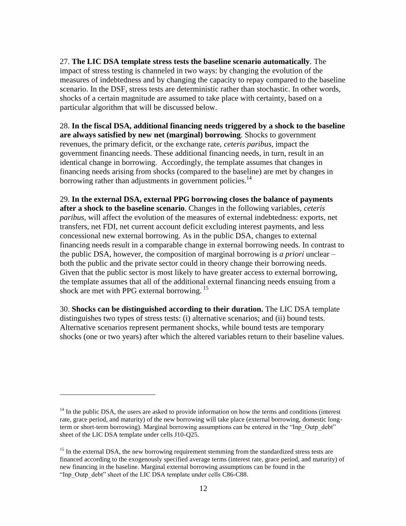
27. The LIC DSA template stress tests the baseline scenario automatically. The
impact of stress testing is channeled in two ways: by changing the evolution of the
measures of indebtedness and by changing the capacity to repay compared to the baseline
scenario. In the DSF, stress tests are deterministic rather than stochastic. In other words,
shocks of a certain magnitude are assumed to take place with certainty, based on a
particular algorithm that will be discussed below.
28. In the fiscal DSA, additional financing needs triggered by a shock to the baseline
are always satisfied by new net (marginal) borrowing. Shocks to government
revenues, the primary deficit, or the exchange rate, ceteris paribus, impact the
government financing needs. These additional financing needs, in turn, result in an
identical change in borrowing. Accordingly, the template assumes that changes in
financing needs arising from shocks (compared to the baseline) are met by changes in
borrowing rather than adjustments in government policies.14
29. In the external DSA, external PPG borrowing closes the balance of payments
after a shock to the baseline scenario. Changes in the following variables, ceteris
paribus, will affect the evolution of the measures of external indebtedness: exports, net
transfers, net FDI, net current account deficit excluding interest payments, and less
concessional new external borrowing. As in the public DSA, changes to external
financing needs result in a comparable change in external borrowing needs. In contrast to
the public DSA, however, the composition of marginal borrowing is a priori unclear –
both the public and the private sector could in theory change their borrowing needs.
Given that the public sector is most likely to have greater access to external borrowing,
the template assumes that all of the additional external financing needs ensuing from a
shock are met with PPG external borrowing. 15
30. Shocks can be distinguished according to their duration. The LIC DSA template
distinguishes two types of stress tests: (i) alternative scenarios; and (ii) bound tests.
Alternative scenarios represent permanent shocks, while bound tests are temporary
shocks (one or two years) after which the altered variables return to their baseline values.
14 In the public DSA, the users are asked to provide information on how the terms and conditions (interest
rate, grace period, and maturity) of the new borrowing will take place (external borrowing, domestic long-
term or short-term borrowing). Marginal borrowing assumptions can be entered in the ―Inp_Outp_debt‖
sheet of the LIC DSA template under cells J10-Q25.
15 In the external DSA, the new borrowing requirement stemming from the standardized stress tests are
financed according to the exogenously specified average terms (interest rate, grace period, and maturity) of
new financing in the baseline. Marginal external borrowing assumptions can be found in the
―Inp_Outp_debt‖ sheet of the LIC DSA template under cells C86-C88.

13
31. The LIC DSA template calibrates the magnitude of the shocks using 10 years of
historical data.16
This default period is used to calculate the historical averages and
associated standard deviation of key macro variables. However, under certain
circumstances, the standardized stress tests may not capture adequately the vulnerabilities
of the country. For instance, structural breaks in the time series (i.e. discovery of oil or a
civil war) or data deficiencies may require a change in the period used for calibration.
Bound tests are calibrated so that the implied outcome for the long-term debt ratio (at a
10-year horizon) has a roughly 25 percent likelihood of occurring.17
18
32. Stress testing should follow an asymmetric approach and be tilted toward
adverse shocks. To check its robustness, the user should stress the baseline with
meaningful adverse shocks i.e. the DSF is interested in downside rather than upside risks.
Thus, while it may occur that stress tests calibrated using 10-year averages and standard
deviations deliver positive shocks, implying an improvement in debt burden indicators,
such shocks could be altered to model downside risks.
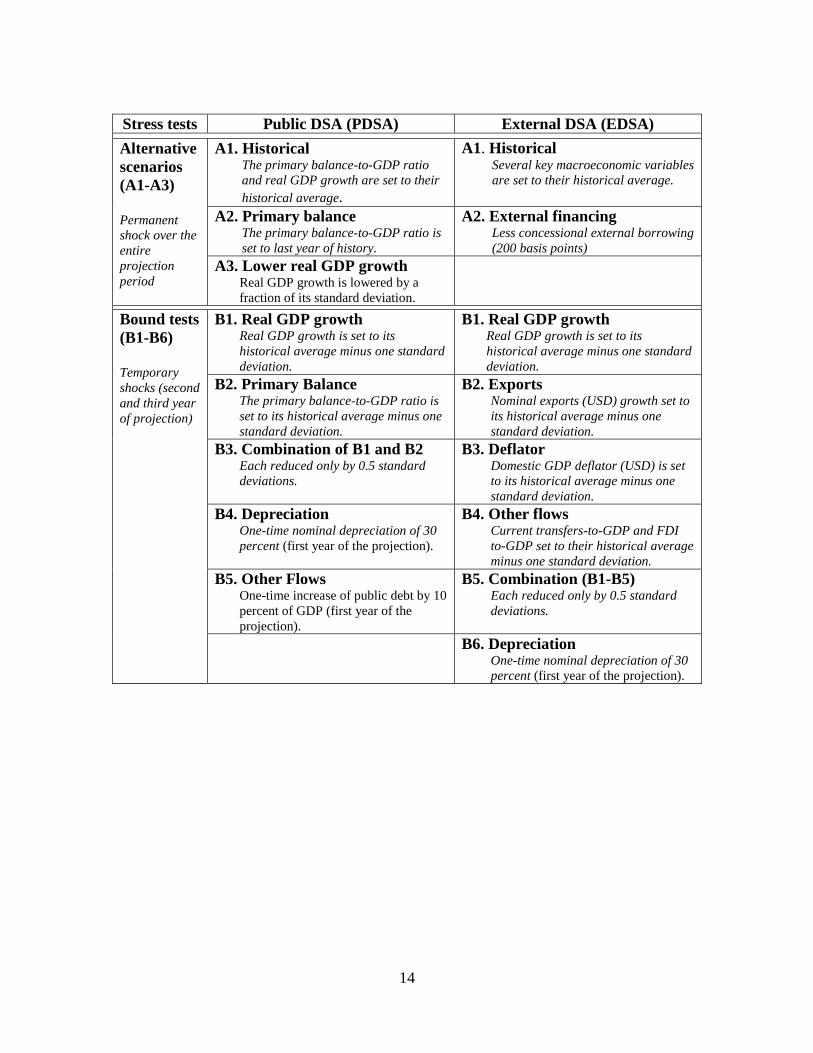
33. The LIC DSA template contains 16 different standardized stress tests in total.
The public DSA (PDSA) comprises 3 alternative scenarios and 5 bound tests; the external
DSA (EDSA) encompasses 2 alternative scenarios and 6 bound tests. To simplify the
description of the stress tests, comparable shocks will be described in the same section.
16 For the fiscal DSA average and standard deviations are calculated in cells AK16-AL55 in the ―fiscal-
baseline‖ sheet. For the external DSA average and standard deviations are calculated in cells B68-P73 in
the ―baseline‖ sheet.
17 See ―Debt Sustainability in Low-Income Countries—Proposal for an Operational Framework and Policy
Implications‖, IMF and IDA, February 2004.
18 Note that, bound tests do not exhibit unsustainable debt dynamics within this framework, unless the
baseline does. Stress tests are constructed in such a way that the interest rate, growth rate, and primary
balance (or current account excluding interest payments) return to their baseline value after the shock
dissipates.
14
Stress tests Public DSA (PDSA) External DSA (EDSA)
Alternative
scenarios
(A1-A3)
Permanent
shock over the
entire
projection
period
A1. Historical The primary balance-to-GDP ratio
and real GDP growth are set to their
historical average.
A1. Historical Several key macroeconomic variables
are set to their historical average.
A2. Primary balance The primary balance-to-GDP ratio is
set to last year of history.
A2. External financing Less concessional external borrowing
(200 basis points)
A3. Lower real GDP growth Real GDP growth is lowered by a
fraction of its standard deviation.
Bound tests
(B1-B6)
Temporary
shocks (second
and third year
of projection)
B1. Real GDP growth Real GDP growth is set to its
historical average minus one standard
deviation.
B1. Real GDP growth Real GDP growth is set to its
historical average minus one standard
deviation.
B2. Primary Balance The primary balance-to-GDP ratio is
set to its historical average minus one
standard deviation.
B2. Exports Nominal exports (USD) growth set to
its historical average minus one
standard deviation.
B3. Combination of B1 and B2 Each reduced only by 0.5 standard
deviations.
B3. Deflator Domestic GDP deflator (USD) is set
to its historical average minus one
standard deviation.
B4. Depreciation One-time nominal depreciation of 30
percent (first year of the projection).
B4. Other flows Current transfers-to-GDP and FDI
to-GDP set to their historical average
minus one standard deviation.
B5. Other Flows One-time increase of public debt by 10
percent of GDP (first year of the
projection).
B5. Combination (B1-B5) Each reduced only by 0.5 standard
deviations.
B6. Depreciation One-time nominal depreciation of 30
percent (first year of the projection).
15
5.1 Shock to real GDP growth (PDSA and EDSA)
There are two temporary shocks (bound test B1 in PDSA and EDSA) and one permanent
shock (alternative scenario A3 in PDSA) to real GDP growth.
Description: Under the temporary shocks (B1), real GDP growth is set at its historical average
minus one standard deviation over the second and third year of the projection period (t+1 and
t+2). Real GDP growth returns to the baseline projection thereafter. Under the permanent shock
(A3), the baseline real GDP growth projection is reduced over the entire projection period by
roughly one-fifth of one standard deviation.19
34. For both the PDSA and the EDSA, the shock to real GDP growth represents a
shock to measures of capacity to repay. The adverse shock to real GDP growth has a
permanent impact on the level of real GDP (Yr) and nominal GDP (Y
n). This is the
consequence of two assumptions: (i) real GDP growth returns to the baseline projection
after the shock; and (ii) inflation remains unchanged, as measured by the GDP deflator.
The decline in nominal GDP (compared to the baseline) has in turn a proportional
negative impact on the nominal level of government revenues because the revenues-to-
GDP ratio is assumed to remain unchanged compared to the baseline.
35. In the PDSA (A3 and B1), the shock to real GDP growth also represents a shock
to the measures of indebtedness (Figure 1). While the real GDP shock affects adversely
nominal revenues, it is not assumed to have an impact on the level of government
spending. Smaller tax revenues with respect to the baseline and unchanged spending
results in a wider non-interest (primary) fiscal deficit and increased financing needs, and
thus additional borrowing. Note that grants are also assumed constant in nominal terms
compared to the baseline, and, thus, increase in GDP terms. In the end, future financing
needs are compounded by new marginal borrowing as it raises future debt servicing costs
(principal and interest payments).
36. In the EDSA, the shock to real GDP growth has no impact on the measures of
indebtedness. Variables affecting the evolution of the measures of indebtedness such as
the level of net FDI inflows or the current account (exports, imports, net current transfers,
other non-interest current account flows and interest payments) remain unchanged
compared to the baseline scenario. With the current account and net FDI unaffected by
the shock, the level of external debt, its NPV, and the level of debt service coincides with
the baseline scenario. In other words, in the EDSA, the shock to real GDP growth affects
debt burden indicators only through the impact on the denominators, that is, nominal
GDP and government revenues.
19
20(baseline)growth GDP real A3) (scenariogrowth GDP Real
STD
16
Figure 1: Negative shock to real GDP growth (PDSA) - impact on the level of gross
financing needs
5.2 Exchange rate depreciation (PDSA and EDSA)
Depreciation shocks are present in both the fiscal and external DSA (bound tests B4 in
PDSA and B6 in EDSA). This reflects the currency mismatch risks between the measures
of capacity to repay (GDP and revenues are in local currency) and the measures of
indebtedness (external debt is denominated in foreign currency).
Description: The 30 percent depreciation shock takes place in the second projection year. During
the third projection year, the change in the nominal exchange rate resumes its path in line with the
baseline scenario. Given that domestic and foreign prices are not affected, the nominal
depreciation can be interpreted as real exchange rate shock.
37. In the EDSA, the nominal depreciation results in a concomitant decline in the
GDP deflator denominated in USD. Changes in the deflator lead to a proportional and
permanent reduction in the value of domestic GDP in US dollars. However, real GDP
growth (LCU) remains unchanged compared to the baseline. In addition, the level of all
the components of the BoP are assumed to be unaffected by the shock. In other words,
the exchange rate shock is a pure valuation shock. As discussed in the previous section
(section 5.1), changes to nominal GDP will impact government revenues (expressed in
foreign exchange) in the EDSA, which represents the denominator, but would not affect
measures of indebtedness. Hence, while the level of external debt is unchanged (measure
of indebtedness), the debt burden indicator is affected by smaller nominal GDP and
government revenues (the capacity to repay). Meanwhile, debt burden indicators based
on exports will remain unchanged compared to the baseline as the exchange rate shock is
assumed not to affect trade.
38. In the PDSA, the measures of repayment capacity (nominal GDP and
government revenues in LCU) are not affected by the exchange rate depreciation. In
addition, government spending (excluding interest payments) or grants do not change
Amortization and interest payments↑
Real GDP
growth shock
Nominal GDP↓
Gov. tax revenues ↓
Primary deficit ↑
Gross financing requirements ↑
New borrowing↑
Real GDP growth is temporarily reduced, inflation in unchanged
Tax-to-GDP ratio is unchanged, the level of grants remains
unchanged
Government spending is unchanged
17
after the depreciation shock. Therefore, the primary deficit remains unchanged after the
depreciation.
39. In the PDSA, the nominal exchange rate depreciation affects only the measures
of indebtedness and composition of new borrowing. The depreciation has two direct
effects on the level and composition of new borrowing (Figure 2): i) in local currency
terms, it increases the cost of servicing the existing stock of foreign currency-
denominated debt (level effect); and ii) the value of planned PPG foreign borrowing is
assumed to remain constant is USD after the depreciation, which implies a larger value of
foreign borrowing in local currency. Given that the primary balance is unchanged in local
currency and foreign borrowing plans are unchanged is USD, the depreciation
effectively leaves the country with more local currency from external borrowing to
finance the same primary balance, , which may reduce net domestic debt (composition
effect).
Figure 2: Exchange rate depreciation (PDSA) - impact on the level of gross financing
needs
5.3 Shock to the primary balance (PDSA)
There are two primary balance shocks in the PDSA: one permanent (alternative scenario
A2) and one temporary (bound test B2).
Description: Under the permanent shock (scenario A2), the primary deficit-to-GDP ratio is set at
a level equivalent to the primary deficit in the first year of the projection over the entire
projection period. This shock is also called the fiscal policy status quo. Under the temporary
shock (bound test B2), the primary deficit-to-GDP ratio is set to equal its historical average minus
one standard deviation during the second and third projection year.
Exchange rate
depreciation
Amortization and interest payments on existing stock of external debt ↑
Value of projected FX borrowing in local currency ↑
New borrowing: financing mix (external and
domestic borrowing)
Planned external borrowing remains unchanged in FX
Primary balance remains unchanged in local currency
Gross financing requirements ↑
Amortization and interest payments↑
18
40. Under both scenarios, it is assumed that the shock to the primary deficit occurs
through changes in primary expenditures, rather than government revenues. The
idea behind the permanent shock (A2) is to present the outcome of no policy changes to
the current fiscal stance. The bound test (B2) demonstrates the impact of a temporary
spending shock. The wider primary deficit increases the gross financing need (Figure 3)
and, thus, public borrowing (external or domestic), which will further increase future
financing needs through additional future interest and amortization payments.
41. Under both scenarios, the deterioration in the debt burden indicators reflects an
increase in the measure of indebtedness, rather than a deteriorating repayment
capacity. Despite an increase in government spending, nominal GDP and government
revenues remain unchanged under both scenarios.
Figure 3: Shocks to the Primary Balance (PDSA) - impact on the level of gross financing
needs
5.4 Shock to the primary balance and real GDP growth (PDSA)
There are two standardized stress tests combining a shock to the primary balance and a
shock to real GDP growth: one permanent (alternative scenario A1) and one temporary
(bound test B3) shock.
Description: Under the permanent shock (alternative scenario A1), the primary balance-to-GDP
ratio and real GDP growth are set to equal their historical average starting in the second year of
the projection and lasting over the entire projection horizon. Under the temporary shock (bound
test B3), real GDP growth and the primary balance-to-GDP ratio are set in second and third year
of the projection to equal their historical averages minus half standard deviation.
42. Both stress tests (alternative scenario A1 and bound test B3) are a combination
of individual shocks discussed above (section 5.1 and 5.2). The deterioration in the
primary deficit in the second and third year of the projection reflects the shock to the
primary balance. Thereafter, the adverse shock to real GDP growth (deterioration in
repayment capacity), which in turn affects adversely nominal government revenues
Primary Deficit↑
Gross financing requirements↑
New borrowing ↑
Tax-to-GDP ratio and grants are constant, government spending increase
Amortization and interest payments↑

19
(through the decline in nominal GDP), leads to a deterioration of the primary deficit and
an increase in gross borrowing requirement (Figure 4).20
The LIC DSA template assumes
an unchanged level of grants implying a larger grant-to-GDP ratio. Note also that under
the combo stress test, the magnitude of the shocks is smaller (½ standard deviation)
compared to the shocks to individual macro variables (1 standard deviation).21
Figure 4: Negative shock to primary balance and real GDP growth - impact on the level
of gross financing needs
5.5 Shock to other debt creating flows (PDSA)
One-off increase in other debt creating flows amounting to 10 percent of GDP reflects a
contingent liabilities shock (bound test B5)
20 Once new borrowing is assumed, the financing requirement will also reflect additional amortization and
interest payments.
21 The shock magnitude under the combo stress test is smaller as the probability that very large shocks hit
the economy simultaneously is likely to be small and the DSF does not attempt to model extreme risks or
scenarios. From a practical perspective, if the combo stress test were of equal size compared to other
individual shocks to the same macro variables, then such individual shocks would always represent subsets
of the large shock from a most extreme scenario perspective. t.
Real GDP
growth↓
Nominal GDP↓
Gov. tax revenues↓
Gross financing requirement↑
Primary deficit ↑
Real GDP growth is reduced, inflation in unchanged
Tax-to-GDP ratio is unchanged
New borrowing↑
Amortization and interest payments↑
Tax-to-GDP ratio is constant, the level of grants is unchanged,
government spending adjust
Gross financing requirement↑t+1
New borrowing↑t+1
Amortization and interest payments↑
20
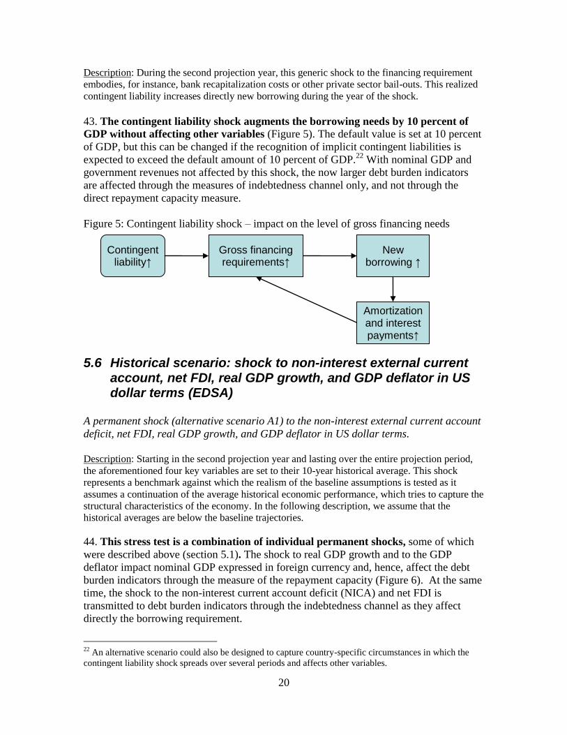
Description: During the second projection year, this generic shock to the financing requirement
embodies, for instance, bank recapitalization costs or other private sector bail-outs. This realized
contingent liability increases directly new borrowing during the year of the shock.
43. The contingent liability shock augments the borrowing needs by 10 percent of
GDP without affecting other variables (Figure 5). The default value is set at 10 percent
of GDP, but this can be changed if the recognition of implicit contingent liabilities is
expected to exceed the default amount of 10 percent of GDP.22
With nominal GDP and
government revenues not affected by this shock, the now larger debt burden indicators
are affected through the measures of indebtedness channel only, and not through the
direct repayment capacity measure.
Figure 5: Contingent liability shock – impact on the level of gross financing needs
5.6 Historical scenario: shock to non-interest external current account, net FDI, real GDP growth, and GDP deflator in US dollar terms (EDSA)
A permanent shock (alternative scenario A1) to the non-interest external current account
deficit, net FDI, real GDP growth, and GDP deflator in US dollar terms.
Description: Starting in the second projection year and lasting over the entire projection period,
the aforementioned four key variables are set to their 10-year historical average. This shock
represents a benchmark against which the realism of the baseline assumptions is tested as it
assumes a continuation of the average historical economic performance, which tries to capture the
structural characteristics of the economy. In the following description, we assume that the
historical averages are below the baseline trajectories.
44. This stress test is a combination of individual permanent shocks, some of which
were described above (section 5.1). The shock to real GDP growth and to the GDP
deflator impact nominal GDP expressed in foreign currency and, hence, affect the debt
burden indicators through the measure of the repayment capacity (Figure 6). At the same
time, the shock to the non-interest current account deficit (NICA) and net FDI is
transmitted to debt burden indicators through the indebtedness channel as they affect
directly the borrowing requirement.
22
An alternative scenario could also be designed to capture country-specific circumstances in which the
contingent liability shock spreads over several periods and affects other variables.
Gross financing requirements↑
Contingent liability↑
New borrowing ↑
Amortization and interest payments↑

21
45. The historical scenario affects the repayment capacity through its impact on
domestic nominal GDP in US dollar. The permanent reduction in real GDP growth and
the change in the domestic GDP deflator in US dollar terms (compared to the baseline
scenario) results in a reduced growth rate of nominal GDP and, therefore, a smaller
nominal GDP. In addition, the historical scenario assumes that all current account
components and government revenues remain unchanged in percent of GDP, with respect
to the baseline. Accordingly the reduction in nominal GDP implies a proportional
reduction in exports and government revenues.
46. Shocks to both the external current account and the net FDI impact the
financing need and, therefore, external borrowing (measure of indebtedness). The
increase in debt leads to an increase in debt service payments as well as the PV of debt.
47. All debt burden indicators are expected to deteriorate, reflecting a decline in the
measure of the capacity to repay (nominal GDP, exports and government revenues) in
conjunction with larger indebtedness, which in turn leads to an increase in PV of debt and
debt service payments.
Figure 6: Key variables set to historical averages - impact on the level of gross financing
needs
t:
t+1:
GDP deflator (in US$)
↓
Nominal GDP ↓
Gov. revenues↓
Real GDP growth
↓
NICAt ↓
Gross financing requirement↑ Debt↑
Amortization, interest↑
Net FDIt ↓
GDP deflator (in US$)
↓
Nominal GDP ↓
Gov. revenues↓
Real GDP growth
↓
NICAt+1 ↓
Gross financing requirement ↑ Debt↑ Net FDIt
+1↓
Export level↓
Export level↓
22
5.7 Shock to terms of foreign financing (EDSA)
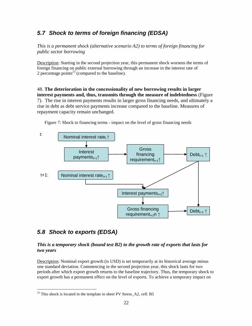
This is a permanent shock (alternative scenario A2) to terms of foreign financing for
public sector borrowing
Description: Starting in the second projection year, this permanent shock worsens the terms of
foreign financing on public external borrowing through an increase in the interest rate of
2 percentage points23
(compared to the baseline).
48. The deterioration in the concessionality of new borrowing results in larger
interest payments and, thus, transmits through the measure of indebtedness (Figure
7). The rise in interest payments results in larger gross financing needs, and ultimately a
rise in debt as debt service payments increase compared to the baseline. Measures of
repayment capacity remain unchanged.
Figure 7: Shock to financing terms - impact on the level of gross financing needs
5.8 Shock to exports (EDSA)
This is a temporary shock (bound test B2) to the growth rate of exports that lasts for
two years Description: Nominal export growth (is USD) is set temporarily at its historical average minus
one standard deviation. Commencing in the second projection year, this shock lasts for two
periods after which export growth returns to the baseline trajectory. Thus, the temporary shock to
export growth has a permanent effect on the level of exports. To achieve a temporary impact on
23
This shock is located in the template in sheet PV Stress_A2, cell: B5
t:
t+1:
Nominal interest ratet ↑
Interest paymentst+1↑
Gross financing
requirementt+1↑
Nominal interest ratet+1 ↑
Interest paymentst+2↑
Debtt+1 ↑
Gross financing requirementt+2n ↑
Debtt+2 ↑

23
the level of the non-interest current account, the level of imports is reduced from the third year
onward of the projection period.
49. The shock to nominal exports growth in dollar terms results in a deterioration of
the current account deficit, and hence affects the measure of indebtedness (Figure 8).
Under this bound test, imports are assumed constant during the shock and adjust
thereafter to assure an external non-interest current account deficit equivalent to the
baseline. The wider external deficit causes a rise in gross financing needs, which elevates
the external debt level. During the second year of the shock, in addition to the decline in
exports, larger debt service payments (amortization and interest payments) stemming
from the higher indebtedness a year earlier contribute to a further rise in gross financing
needs.
50. A downward adjustment in the level of imports ensures that the non-interest
current account deficit reverts to the baseline trajectory after the two-period shock.
This adjustment in imports is permanent and in line with permanently lower export levels
following the shock (compared to the baseline). External debt is, nevertheless, larger
throughout the projection period due to larger current account deficits. The increase in
debt service payments leads to an increase in the NPV of external debt.
51. The decline in exports does not have an impact on the level of nominal GDP, nor
government revenues. However, all debt burden indicators will be adversely impacted
by a negative shock to exports through an increase in indebtedness. Debt burden
indicators using exports as a measure of capacity to repay will show a greater deterioration
given the reduction in exports.
Figure 8: Two-year shock to exports growth - impact on the level of gross financing needs
t:
t+1:
t+2:
Export growth↓ NICAtn
↑ Gross financing
requirement↑ Debtt↑
Amortizationt+1, interest paymentst+1↑
Export growth↓ NICAt+1n ↑ Gross financing requirement t+1↑
Debtt+1↑
Export unchanged
NICAt+2n
unchanged
Amortizationt+2, interest t+2↑
Gross financing requirementt+2↑
Debtt+2↑ Imports ↓
24
5.9 Shock to domestic GDP Deflator in dollar terms (EDSA)
This is a temporary shock (bound test B3) that reduces the growth rate of the domestic GDP
deflator expressed in US dollar terms
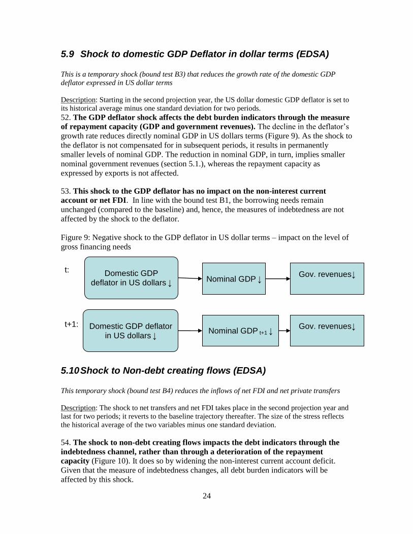
Description: Starting in the second projection year, the US dollar domestic GDP deflator is set to
its historical average minus one standard deviation for two periods.
52. The GDP deflator shock affects the debt burden indicators through the measure
of repayment capacity (GDP and government revenues). The decline in the deflator’s
growth rate reduces directly nominal GDP in US dollars terms (Figure 9). As the shock to
the deflator is not compensated for in subsequent periods, it results in permanently
smaller levels of nominal GDP. The reduction in nominal GDP, in turn, implies smaller
nominal government revenues (section 5.1.), whereas the repayment capacity as
expressed by exports is not affected.
53. This shock to the GDP deflator has no impact on the non-interest current
account or net FDI. In line with the bound test B1, the borrowing needs remain
unchanged (compared to the baseline) and, hence, the measures of indebtedness are not
affected by the shock to the deflator.
Figure 9: Negative shock to the GDP deflator in US dollar terms – impact on the level of
gross financing needs
5.10 Shock to Non-debt creating flows (EDSA)
This temporary shock (bound test B4) reduces the inflows of net FDI and net private transfers
Description: The shock to net transfers and net FDI takes place in the second projection year and
last for two periods; it reverts to the baseline trajectory thereafter. The size of the stress reflects
the historical average of the two variables minus one standard deviation.
54. The shock to non-debt creating flows impacts the debt indicators through the
indebtedness channel, rather than through a deterioration of the repayment
capacity (Figure 10). It does so by widening the non-interest current account deficit.
Given that the measure of indebtedness changes, all debt burden indicators will be
affected by this shock.
Domestic GDP deflator in US dollars ↓ Nominal GDP ↓
t:
t+1:
Gov. revenues↓
Domestic GDP deflator in US dollars ↓
Nominal GDP t+1
↓ Gov. revenues↓

25
Figure 10: Negative shock to non-debt creating flows - impact on the level of gross
financing needs
5.11 Shock to real GDP, exports, GDP deflator, and non-debt creating flows (ESDA)
This temporary shock (bound test B5) is the most comprehensive stress test in the
template as it combines shocks to five variables: real GDP (B1) and exports growth (B2),
the GDP deflator (B3), and net private transfers and FDIs (B4).
Description: This shock embodies the simultaneous impact of four bound tests (B1-B4)
presented earlier (sections 5.1, 5.8, 5.9, 5.10). As opposed to other bound tests, however, the
historical averages under this shock are reduced by one-half rather than a full standard deviations.
Similar to other stress tests, this shock starts in the second projection period and lasts over two
periods.
55. This shock deteriorates all measure of the capacity to repay through the decline
in real GDP, the deflator, and exports (Figure 11). The temporary decline in real GDP
growth and the growth of the GDP deflator in US dollar terms translates into a transitory
reduction in nominal GDP growth in U.S. dollars. However, because the temporary
deceleration in real growth and inflation (compared to the baseline) are not compensated
by increases in subsequent years, the temporary shock to nominal GDP growth has a
permanent impact on the level of nominal GDP. Consequently, nominal GDP in this
stress test will be smaller than in the baseline scenario over the entire projection period.
As in previous bound tests, the share of government revenues in GDP remains unchanged
compared to the baseline. As a result, government revenues will also be permanently
smaller compared to the baseline scenario. Finally, by reducing temporarily the rate of
growth in exports (compared to the baseline), the shock permanently reduces the level of
exports.
Non-debt creating flow ↓ (Current Transfers and net
FDI)
Gross Financing Requirement↑
Debtt↑ t:
t+1: Gross Financing Requirementt+1↑
Amortizationt+1, interest paymentst+1↑
Non-debt creating flow ↓
(Current Transfers and net FDI)
Debtt+1↑

26
56. The decline in exports growth, net private transfers and FDIs worsens the
measures of indebtedness. The deceleration in the rate of growth of exports and the
reduction in net transfers and FDI widen the non-interest current account deficit in
absolute terms compared to the baseline. After the shock dissipates, net transfers revert to
their baseline values in absolute terms, and imports decline to help the trade balance
return to the baseline value in absolute terms.
57. All debt burden indicators are expected to worsen compared to the baseline
scenario. This reflects the adverse impact of this shock on all measures of repayment
capacity (GDP, revenues and exports) as well as on the measures of indebtedness (PV of
debt and debt service).
Figure 11: Negative combination shock - impact on the level of gross financing needs
t:
t+1:
Domestic GDP
deflator in US dollars↓
Nominal GDP↓ Gov. revenues↓
Real GDP growth↓
Exportst ↓
Gross financing requirement↑ Debtt↑
AMTt+1, INTt+1↑
Net Transfers
↓
Domestic GDP
deflator in US dollars↓
Nominal GDP ↓ Gov. revenues↓
Real GDP growth ↓
Exportst+1 ↓
Gross financing requirement t+1↑ Debtt+1
Net FDIt+1
↓
t+2:
AMTt+2, INTt+2↑
Exportst+2↓
Gross financing requirementt+2↑ Debtt+2↑
Importst+2↓
Trade Balancet+2 unchanged
Domestic GDP
deflator in US dollars↓
Nominal GDP ↓ Gov. revenues↓
Real GDP growth ↓

27
6 Conclusion
58. This technical note describes in detail the intuition and propagation of
deterministic standardized stress tests in the LIC DSA template using an analytical and
graphical approach. It is intended to aid technical staff in low income countries as well as
country teams at the IMF and WB by providing the intuition as well as mechanics of
stress testing. This should enhance the understanding of the shocks in the DSF and help
improve the elaboration of debt sustainability exercises in low income countries.
28
7 References
Burnside, Craig ed. (2005). ―Fiscal Sustainability in Theory and Practice – A Handbook‖,
The World Bank, Washington D.C.
Kraay, Aart and Vikram Nehru (2004). ―When is External Debt Sustainable?‖. World
Bank Policy Research Paper No. 3200.
Ley, Eduardo (2007). ―Fiscal Policy for Growth‖, PRMED Knowledge Brief, June
World Bank and IMF (2010). ―Staff Guidance Note on the Application of the Joint Bank-
Fund Debt Sustainability Framework for Low-Income Countries‖.
World Bank and IMF (2008). ―Staff Guidance Note on the Application o f the Joint
Fund-Bank Debt Sustainability Framework for Low-Income Countries‖.
World Bank and IMF (2005). ―Operational Framework for Debt Sustainability
Assessments in Low-Income Countries-Further Considerations‖.
World Bank and IMF (2004). ―Debt-Sustainability in Low-Income Countries-Proposal
for an Operational Framework and Policy Implications‖.
World Bank and IMF (2004a). ―Debt Sustainability in Low-Income Countries-Further
Considerations on an Operational Framework and Policy Implications‖.