BPEA Conference Drafts, September 7–8, 2017

Strengthening and Streamlining Bank Capital Regulation

Robin Greenwood, Harvard Business School

Samuel G. Hanson, Harvard Business School

Jeremy C. Stein, Harvard University

Adi Sunderam, Harvard Business School

Conflict of Interest Disclosure: Jeremy C. Stein is on the board of directors for the Harvard

Management Company, an unpaid position. In the past year, he has given paid speeches for

Barclays, Citigroup, Goldman Sachs, and J.P. Morgan, and has served as a consultant to Key

Square Capital Management. A full list of Stein’s compensated and significant non-compensated

activities since 2006 is available on his website, https://scholar.harvard.edu/stein/pages/outside-

activities. With the exception of the aforementioned, the authors did not receive financial support

from any firm or person for this paper or from any firm or person with a financial or political

interest in this paper. With the exception of the aforementioned, they are currently not officers,

directors, or board members of any organization with an interest in this paper. No outside party

had the right to review this paper prior to circulation.

ROBIN GREENWOOD Harvard Business School and NBER

SAMUEL G. HANSON

Harvard Business School and NBER

JEREMY C. STEIN Harvard University and NBER

ADI SUNDERAM

Harvard Business School and NBER

Strengthening and Streamlining Bank Capital Regulation∗

August 2017

ABSTRACT: We propose three core principles that should inform the design of bank capital regulation. First, wherever possible, multiple constraints on the minimum level of equity capital should be consolidated into a single constraint. This helps to avoid a distortionary situation where different constraints bind for different banks performing the same activity. Second, while a regulatory framework that relies primarily on minimum capital ratios is appropriate for normal times, such a framework is inadequate in the wake of a large negative shock to the system. Following an adverse shock, it becomes critical to emphasize dynamic resilience, which involves forcing banks to actively recapitalize—i.e. regulation needs to focus on getting banks to raise new dollars of equity capital, rather than just maintaining their capital ratios. Third, the best way to deal with the inevitable gaming of any set of ex ante capital rules is not to propose further rules, but rather to allow the regulator sufficient flexibility to address unforeseen contingencies ex post. We use these principles to suggest a number of modifications to the current set of risk-based capital requirements, to the leverage ratio, and to the Federal Reserve’s stress-testing framework.

∗ Draft prepared for Brookings Papers on Economic Activity, September 2017 meeting. We thank Vickie Alvo, Francisco Covas, Jan Eberly, Bev Hirtle, Anil Kashyap, Don Kohn, Anna Kovner, Nellie Liang, Andrew Metrick, Sandie O’Connor, Dan Tarullo, Mark Van Der Weide, James Vickery, and Matt Zames for helpful conversations and feedback. Outside-activity disclosures are available at http://people.hbs.edu/rgreenwood/outside_activities.pdf, http://www.people.hbs.edu/shanson/Disclosure_statement_SH.pdf, https://scholar.harvard.edu/stein/pages/outside-activities, and http://people.hbs.edu/asunderam/outside_activities.pdf. An internet appendix for the paper is available at http://people.hbs.edu/shanson/regreform2017_IA.pdf.

1

In the wake of the global financial crisis of 2008-09, financial regulation has undergone a dramatic

overhaul, both in the U.S. and elsewhere. There are many elements to the new regulatory regime,

including enhanced capital requirements and stress testing, liquidity rules, resolution planning,

margin and clearing requirements for derivatives transactions, and much more. With the bulk of

the rulemaking and implementation now nearly complete, it is a natural time to take stock of the

changes: to ask whether the new regulations are working as hoped, how they are meshing with one

another, and what the unintended consequences and other inefficiencies might be.1

In this paper we develop some basic principles that can be used to assess the efficiency of

those parts of the regulatory regime that are most directly tied to bank capital, including the

standard risk-based Basel III capital requirements, the leverage ratio, and the Federal Reserve’s

stress-testing process. While these are far from being the whole regulatory toolkit, they are among

the most important pieces of it, and these elements alone have become very complex. So focusing

our analysis on just capital regulation leaves us with many questions to address, while at the same

time allowing us to bring a relatively parsimonious conceptual framework to bear.

Although we examine a number of aspects of regulatory design in what follows, we should

be clear at the outset that there is one central question that we do not engage with: how much

equity capital the banking system should have in the aggregate. This question has already been the

subject of a great deal of academic and policy research, and given the state of play, and the

available data, we don’t have much new to add here.2 For what it’s worth, our reading of this

previous work leads us to conclude that current levels of capital in the U.S. banking industry are

near the lower end of what would seem to be a generally reasonable range. That is, we think it

would be a mistake if bank capital was allowed to decline to any meaningful extent, and we suspect

that adding a few more percentage points to risk-based capital ratios, especially for the largest

banks, would be socially beneficial.3 However, our focus here is on how, given an overall target

for the capitalization of the banking system, one can implement this target in a manner that best

1 See Duffie (2016), Greenwood, Hanson, Stein, and Sunderam (2017), and Liang (2017a) for recent assessments of the post-crisis financial regulatory regime. 2 See, for example, Basel Committee on Banking Supervision (2010), Hanson, Kashyap and Stein (2011), Admati, DeMarzo, Hellwig, and Pfleiderer (2013), Baker and Wurgler (2015), Sarin and Summers (2016), Federal Reserve Bank of Minneapolis (2016), Firestone, Lorenc and Ranish (2017), Cline (2017), and Goldstein (2017). 3 Here we are in close agreement with Tarullo (2017), who writes: “This assessment….suggests strongly that a reduction in risk-based capital requirements for the U.S. G-SIBs would be ill-advised. In fact, one might conclude that a modest increase in these requirements—putting us a bit further from the bottom of the range—might be indicated.”

2

aligns incentives for efficient lending and risk-taking, and minimizes other distortions. By analogy,

this is akin to taking the government’s target for tax revenues as given, and asking how to design

a tax system that most efficiently raises the desired amount of revenues.

We frame our analysis by laying out a simple model of optimal bank regulation. The model

is designed to capture the market failures that create a need for bank capital requirements in the

first place.4 The spirit of the exercise is to then ask which specific features of the more elaborate

post-crisis regime can be seen as logically consistent with this overarching approach to regulation,

and which features seem to be at odds with it. The model specifies an objective function for both

a profit-maximizing bank and for a benevolent social planner, makes clear how these objectives

diverge, and then asks how the social optimum can be decentralized with a set of capital rules.

A few key messages emerge from the model. First, in a “normal times” steady state, and

under certain intuitive conditions, the social optimum can be implemented with a single

requirement that each bank maintain a sufficient ratio of equity to risk-weighted assets, provided

the risk weights are chosen appropriately. This result is unsurprising, since the model is built to

rationalize a system of risk-based capital requirements. Second, requiring different banks to

maintain different ratios of equity to risk-weighted assets, as Basel III does with its capital-ratio

surcharges for globally significant “G-SIB” banks, can easily be rationalized within the model.

However, crucially, we show that the same economic logic does not support having

multiple independent constraints on bank equity ratios—as is the case when, e.g. banks have to

separately satisfy minimum values for their risk-based capital ratios, their leverage ratios, and their

post-stress capital ratios. This is because when banks have heterogeneous business models,

different constraints can bind in equilibrium for different banks. As a result, two different banks

can face different relative risk weights when performing the same two activities, which distorts

their behavior, just as would happen if different non-financial firms faced different relative

marginal tax rates for the same two activities. We undertake some crude empirical exercises which

suggest that these distortions can be quantitatively significant, and have already had an impact on

bank capital allocation. This leads to our first core design principle, which is that wherever

4 Indeed, one can view our model as an attempt to formalize the view of bank capital regulation that is implicit in many recent official sector documents, including Basel Committee on Banking Supervision (2010, 2015) and Federal Reserve Board of Governors (2015).

3

possible, multiple constraints on the minimum level of equity capital should be consolidated into

a single risk-based constraint.

To be clear, we are only arguing for a reduction in the number of constraints on a single

item, namely bank equity capital. We are not saying that multiple constraints on multiple different

items are undesirable. Thus, for example, a separate liquidity coverage ratio, which specifies that

a bank hold a minimum amount of high-quality liquid assets, need not create any distortions

alongside a binding capital ratio.5

Next, stepping outside of the formal model, we discuss how regulators can best respond to

the inevitable gaming of any rules that they write down. A natural instinct when seeing that one

particular rule (say a risk-based capital requirement) has been arbitraged is to propose another rule

that the historical data suggests would have worked better. This, in part, is the logic invoked by

those arguing for a more prominent role for a non-risk-based leverage ratio requirement. But it is

useful to bear in mind the wisdom in Goodhart’s (1975) law: “Any observed statistical regularity

will tend to collapse once pressure is placed upon it for control purposes.”6 In other words, any

rule, once codified ex ante, will tend to be arbitraged, and this problem cannot be easily addressed

by proposing more rules. Rather, a second principle is that regulators should explicitly aim to take

an incomplete contracting approach, filling in certain contingencies only ex post, once they have

observed how banks are responding to the existing set of rules. As we argue in more detail below,

this somewhat abstract-sounding principle can provide useful concrete guidance for the design of

the annual stress tests.

Finally, we use the model to explore optimal regulation away from the steady state, when

the banking system has been hit with a negative shock that reduces its capital base below the

natural long-run level. We show that, as long as there are flow costs to raising new external equity,

ratio-based capital requirements are not sufficient to implement the first best. Rather, in addition

to specifying capital ratios, the regulator must also compel banks to recapitalize, i.e. to raise new

dollars of outside equity, above and beyond what they would voluntarily do on their own. Thus,

our third design principle is an emphasis on what we call dynamic resilience: in the wake of an

adverse shock, the ability of regulators to implement a prompt recapitalization of the banking

5 By analogy to Pigouvian taxation, we would consider it to be a problem if different firms faced different tax rates on their carbon emissions, but not if there was one uniform tax for carbon emissions and another one for sulfur emissions. 6 This is similar to the Lucas (1976) critique.

4

system is at least as important as setting the exact value of the capital ratio in normal times. This

is in many ways an obvious point, but one that has been under-appreciated in much of the work in

this area, which has been more concerned with calibrating static optimal capital ratios.7

The remainder of the paper proceeds as follows. We start in Section I with a brief primer

on the key elements of the U.S. capital regime, going light on the details and saying (hopefully)

just enough about the general structure of the rules to allow the reader to grasp the important

conceptual issues that arise. In Sections II and III we provide an overview of our theoretical model,

as well as the associated measurement exercises. These are used to motivate our three core design

principles: consolidating constraints, taking an ex post approach to dealing with regulatory

arbitrage, and being mindful of dynamic resilience. We then apply these core principles in Section

IV, using them to develop a number of concrete suggestions for modifying the current risk-based

capital requirements, the leverage ratio, and the Federal Reserve’s stress-testing framework. We

conclude in Section V by noting some of the caveats and tradeoffs associated with our approach.

I. A Primer on the Key Components of the Bank Capital Regime It is hard to overstate the complexity of the current system of bank capital regulation in the U.S.

The largest banks have to comply with at least ten distinct capital requirements, as well as liquidity

requirements and many other rules.8 Moreover the requirements vary with bank size and other

characteristics. Even a partial summary of all of the rules would take more space than we have for

this paper, and would distract from the underlying logic of our argument.9 So in what follows, we

take a highly stylized approach to describing the rules, focusing on a small number that are

particularly important and illustrative, and blurring many distinctions that are not conceptually

7 Though see Sarin and Summers (2016) for an important recent exception. 8 Large banks in the U.S. are subject to minimal requirements for (1) the ratio of Tier 1 capital to average total assets (the “leverage ratio”), (2) the ratio of Tier 1 capital to total leverage exposure (the “supplemental leverage ratio”), (3) the ratio of Tier 1 capital to risk-weighted assets (the “Tier 1 risk-based ratio”), (4) the ratio of Tier 1 common equity to risk-weighted assets (the “CET1 ratio”), (5) the ratio of total capital to risk-weighted assets (the “total risk-based ratio”). Since banks must satisfy a pre-stress and post-stress version of each of these five requirements, there are a total of ten different capital requirements. In addition, under the Dodd-Frank Act’s Collins Amendment, large U.S. banks must compute their risk-weighted assets using both a “standardized approach” and using internal models (the “advanced approach”) and must use the higher of these two figures when computing their three pre-stress risk-based capital ratios. If one counts these as separate requirements, this raises the total number of capital requirements to 13. And, this figure does not count a number of other regulatory constraints that do not apply to bank capital, such as the Liquidity Coverage Ratio, the Net Stable Funding Ratio, and many others. 9 See Goldstein (2017) for a comprehensive description of the current U.S. capital regime.

5

important for our purposes. We apologize to the expert readers who will no doubt spot a number

of omissions and inconsistencies in what follows.10

I.A. Conventional Risk-based Capital Requirements Risk-based capital requirements have been a staple of bank regulation since the 1988 Basel

Accord. Simply put, a risk-based requirement says that a bank must maintain equity capital E equal

to at least some minimal fraction of its risk-weighted assets, i.e., it must have / RBCE RWA k≥ where

RBCk is the risk-based capital requirement, and RWA denotes risk-weighted assets, which in turn

are defined by1

Ni ii

RWA w A=

=∑ where wi is the risk weight on asset category i. This can be re-

written as 1

.NRBC i ii

E k w A=

≥ ×∑ The bottom line is that under the risk-based capital regime, the

capital charge Ki for asset category i—that is, the amount of incremental equity a constrained bank

must hold for an incremental dollar of asset i—is given by:

( ) .i RBC iK RBC k w= × (1)

In the post-crisis U.S. regime, the Tier 1 capital ratio RBCk is the sum of four components:

a baseline value of 6%; a so-called “capital conservation buffer” of 2.5%; a “countercyclical capital

buffer” which can in principle vary over time but which is currently set at 0%; and a bank-specific

“G-SIB surcharge,” which is applied only to the largest globally significant institutions, and which

varies depending on the bank in question.11 Thus, for a smaller non-G-SIB, RBCk = 8.5%, while for

J.P. Morgan, which currently has the largest surcharge of 3.5%, RBCk = 12.0%.12 G-SIB surcharges

began being phased in as of January 2016, and will be in full force by January 2019.

10 For an overview of the Basel III reforms see http://www.bis.org/bcbs/basel3/b3summarytable.pdf. Many of these reforms are being gradually phased in over time and will not fully take effect until 2019. For a summary of the phase- in arrangements see http://www.bis.org/bcbs/basel3/basel3_phase_in_arrangements.pdf. 11 G-SIB surcharges for individual banks in the U.S. are: 3.5% for J.P. Morgan; 3% for Bank of America, Citigroup, and Morgan Stanley; 2.5% for Goldman Sachs; 2% for Wells Fargo; and 1.5% for Bank of New York Mellon and State Street. (The specific G-SIB surcharges are available from Schedule A of form FFIEC 101). These Federal Reserve-imposed surcharges exceed the Basel III-suggested surcharges reported by the Financial Stability Board, and have been referred to by many as being “gold-plated.” 12 To simplify the discussion, throughout this paper we refer to constraints on so-called Tier 1 capital as if they are constraints on common equity. In reality, Tier 1 capital also includes small amounts of other instruments, such as preferred stock and non-controlling interests. There are actually separate requirements for Tier 1 capital and common equity, with the latter being somewhat lower than the numbers we cite in the text. For example, the common equity requirement for a non-G-SIB, inclusive of the capital conservation buffer, is 7%, not 8.5%.

6

The risk weights for different asset categories can be determined in a number of ways.

Under the original 1988 Basel I Accord, bank assets were broken into five broad risk categories,

with risk weights ranging from 0% (e.g., for claims on OCED government debt) to 100% (e.g., for

all C&I and consumer loans). Over time regulators became concerned that these Basel I weights

were not sufficiently sensitive to risk within the broad buckets—e.g., a C&I loan to a AAA-rated

firm would receive the same risk weight as a loan to a CCC-rated firm—giving banks incentives

to gravitate toward riskier loans within each bucket. Thus, in 2004, regulators agreed on a revised

framework for computing more sensitive risk weights, known as the Basel II Accord. Under Basel

II, risk weights can either be determined using a rules-based “Standardized Approach” or a model-

based “Internal Ratings Based Approach.” The Standardized Approach, which was to be used by

smaller banks, sought to replace the broad Basel I buckets with a more granular set of buckets.13

The Internal Ratings Based (IRB) Approach, to be used by large banks, would compute model-

based risk weights using banks’ own internal assessments of the probability of default and loss-

given-default for different loans.

However, concerns about relying solely on the internal, model-based approach grew after

the crisis and these concerns were enshrined in the 2010 Dodd-Frank Act. Thus, U.S. bank holding

companies with more than $250 billion in assets (or $10 billion in foreign assets) are now required

to compute their risk-weighted assets using both the Standardized Approach and the IRB Approach

and to base their capital ratios on the larger of these two figures. All other U.S. bank holding

companies use only the Standardized Approach.

Notably, the risk weights for certain assets can be very low, or even zero, under both Basel

II approaches. For example, a bank’s holdings of Treasury securities carry a zero risk weight and

hence a zero capital charge. The capital charge is also zero when a bank makes a repo loan to

another counterparty that is fully collateralized by Treasuries.

I.B. The Leverage Ratio Loosely speaking, a leverage-ratio requirement is like a simplified version of a risk-based

requirement, in which all the risk weights are set to one, so that equity is constrained to be some

13 The drafters of Basel II proposed tying these standardized risk weights to credit ratings from credit rating agencies like Moody’s and S&P. Following the financial crisis this became controversial, especially in the U.S. where the Dodd-Frank Act forbade financial regulators from making use of credit ratings. As a result, the exact implementation of the Basel II approach varies considerably across countries.

7

minimal fraction of total (unweighted) balance-sheet assets. Leverage ratio requirements were

substantially stiffened for the biggest banks as part of the post-crisis reforms, to the extent that—

as we will show below—they have become a binding or near-binding constraint for many large

banks. Under the so-called Supplementary Leverage Ratio (SLR) rule, banks must maintain

/ SLRE A k≥ , where A is total un-risk-weighted assets.14 Currently for G-SIBs the required ratio is

5%SLRk = , while for non-G-SIBs with assets over $250 billion it is 3%SLRk = . Thus under the

SLR, the capital charge for any asset category i is given by:

( ) .i SLRK SLR k= (2)

That is, for a bank constrained by the SLR, each incremental dollar of any asset requires kSLR

dollars of additional equity.

The contrast between the SLR and the risk-based capital approach is particularly stark in

the case of low-risk assets like Treasury securities. As noted above, these assets face a capital

charge of zero under a risk-based regime, but for a G-SIB, they face a capital charge of 5% under

the SLR. Given this divergence, it is interesting to ask what led regulators to impose much stricter

un-risk-weighted leverage requirements like the SLR in the wake of the crisis. In the period leading

up to its adoption, advocates of the SLR argued that it should play a more prominent role by

pointing to a several problems that they felt were a consequence of a pre-crisis capital framework

that relied almost exclusively on risk-based ratios.

First, risk-based requirements were said to be overly complicated, with risk weights that

were vulnerable to gaming—particularly when, under certain advanced-approach methodologies,

these risk weights could be determined using banks’ own internal models.15 Second, and relatedly,

many banks that failed or came close to failure in 2008 and 2009 looked perfectly healthy

according to the risk-based metrics, while in some of these cases a leverage ratio tended to do a

14 We are over-simplifying: the denominator in the SLR is not literally just the sum of all on-balance sheet assets. It also includes a term designed to aggregate a bank’s off-balance-sheet exposures. However, for the purposes of computing a marginal capital charge for an on-balance-sheet loan category, this term is not relevant, so we ignore it here. It should also be noted that while banks under $250 billion in assets are not required to comply with the SLR, they are required to comply with a more basic version of a leverage ratio that does not make any adjustment for off-balance sheet exposures. 15 Haldane and Madouros (2012) argue that the large number of risk weights under the Basel II standard, together with the move to using banks’ own internal models to set these weights, provided “near-limitless scope for arbitrage.” Behn, Haselmann, and Vig (2016) document evidence of such gaming, using German banks’ responses to the staggered introduction of internal model-based regulation.

8

better job of predicting distress.16 And third, it seems hard to defend the literally zero risk weights

that the risk-based regime places on some sovereign securities.17

We think that all three of these concerns are absolutely valid, and need to be taken seriously

in the design of any capital regime. However, as we explain below, it is something of a non-

sequitur to conclude that an enhanced leverage-ratio requirement is the right response to the

concerns. For example, one can modify the risk-weighting methodology so as to place less reliance

on models—and also raise the risk weights on sovereign securities above zero—without going to

the extreme of setting all risk weights identically equal to one, as the SLR does.

Moreover, in spite of its simplicity, there is nothing manipulation-proof about a leverage-

ratio regime; indeed it is easily gamed by adding more high-risk assets and shedding low-risk

assets.18 So even if the leverage ratio was in fact predictive of bank distress at a time when it was

not an item of as much interest to regulators, Goodhart’s law cautions against extrapolating any

such conclusions to a new environment in which it plays a more central role in regulation. If the

SLR becomes the test that many banks start to study for, we strongly suspect that it will lose much

of its predictive content, just as the risk-based ratio did in the pre-crisis period. Thus if the goal is

to mitigate the incentives for regulatory arbitrage, another approach will be needed.

I.C. Stress Testing Since 2011, the Federal Reserve has conducted an annual exercise known as the

Comprehensive Capital Analysis and Review, or CCAR, on U.S. bank holding companies with

assets exceeding $50 billion. This CCAR process, informally known as the “stress tests,” has

16 Several studies have shown that leverage ratios fared better as predictors of crisis-period performance than did risk-weighted ratios. These include Haldane and Madouros (2012); Demirguc-Kunt et al (2010); and Estrella et al (2000). 17 According to the standardized approach, AAA and AA sovereign credits receive zero risk weights, but national regulators have discretion to set lower, even zero, risk weights for exposures to the local sovereign. Although a zero risk weight for U.S. Treasuries may seem only to be a bit of a stretch (at least in terms of default risk, if not interest rate risk risk), note that the same approach to risk weighting was used in other countries as well, leading to outcomes that were more obviously at odds with common sense, such as a zero risk weight for Greek government bonds (Acharya and Steffen (2015)). 18 Indeed, concerns that banks were gaming overly-simple leverage ratios played an important role in the advent of risk-based capital ratios in the late 1980s. In 1981, U.S. regulators first introduced formal capital requirements based on a leverage ratio—equity capital divided by total assets. Worries soon arose that these risk-insensitive capital requirements were leading banks to substitute away from low-risk, liquid assets and towards high-risk assets and off-balance sheet assets. In response, the Federal Reserve, FDIC, and OCC all proposed risk-based capital standards in 1986, which were then adopted internationally in the 1988 Basel I Accord (Wall (1989), Federal Deposit Insurance Corporation (1997)).

9

become a cornerstone of the current bank capital regulation regime. The CCAR has both

qualitative and quantitative aspects, but for our purposes we will focus primarily on the latter.19,20

In the CCAR, the Fed spells out both an “adverse” and a “severely adverse” economic scenario,

each involving specified declines in GDP growth, increases in unemployment, widening credit

spreads, falling stock prices, etc. The Fed then models, in highly granular detail, how these

economic scenarios will affect each bank’s loan losses and profitability over a two-year forward-

looking horizon.

The quantitative part of the stress tests involve a set of constraints that stipulate that after

taking account of these stress losses, and any offsetting profits, as well as their planned payouts to

shareholders via dividends and repurchases, each bank must still be able satisfy a number of

minimum requirements on both their risk-based capital ratios and their leverage ratios. To keep

the exposition manageable, we will concentrate on two of these: the post-stress Tier 1 capital ratio,

and the post-stress Tier 1 SLR.

The post-stress Tier 1 capital ratio requires that, after taking into account the losses in the

severely adverse scenario, as well as any planned payouts, a bank must still satisfy a risk-based

capital requirement of ,RBC STRESSk , which is currently set at 6%. Analogously, the post-stress

supplemental leverage ratio requires that post-stress, a bank must still satisfy a non-risk-based

supplemental leverage requirement of ,SLR STRESSk , which is currently set at 3%.

Unlike the conventional risk-based capital and leverage ratio rules, neither of these post-

stress capital requirements come with a set of explicitly spelled-out risk weights or capital charges.

Nevertheless, with a bit of algebra, it is possible to back out the effective capital charges that are

implicit in the post-stress requirements, under the assumption that either one is a binding

19 Technically, the Fed uses its stress testing process as an input to two different exercises, the CCAR and the Dodd-Frank Act Stress Test, or DFAST. The assumptions about loan losses and pre-provision net revenue (PPNR) are the same in DFAST and CCAR. The two main differences between DFAST and CCAR are that: (i) the CCAR incorporates individual banks’ proposed plans for dividends and share repurchases rather making mechanical assumptions about payouts as in DFAST; and (ii) in CCAR supervisors make a qualitative assessment of banks’ practices for risk management, internal controls, and governance; (Liang 2017b). Our empirical analysis uses post-stress capital ratios from the CCAR as a measure of the tightness of various constraints, but takes loss estimates from the DFAST, since this is the only place that loss assumptions are disclosed. 20 In addition to this annual stress test run by the Federal Reserve, all U.S. bank holding companies with assets over $10 billion are required to carry out company-run stress tests at least once each year. Somewhat confusingly, since these biannual company-run tests were mandated under the Dodd-Frank Act, they are often also referred to as the “DFAST stress tests.”

10

constraint. We do this imputation in precise detail in the Appendix; here we just state approximate

versions of the results that make the economic intuition easier to see.

For the post-stress Tier 1 capital ratio requirement, we show that the implicit capital charge

on loan category i can be roughly approximated as:

,( , )i RBC STRE iSS iK RBC STRE LS k w RS N+≈ × , (3)

where wi is the risk weight associated with the standard risk-based regime (i.e. the same value as

in equation (1)), and where NLRi is the net after-tax loss rate on loan category i over the two-year

horizon in the severely adverse scenario, taking account of the fact that, even in such a scenario,

gross loan losses in any category are offset to some extent by the incremental pre-loss net revenue

(i.e., pre-provision net revenue) that accrues in this category over the forecast period.21

Equation (3) can be rewritten as:

,( , ) RBCi RBC STRESS iK RBC STRESS k ω≈ × (3a)

where we have defined a set of implicit risk weights RBCiω for the post-stress Tier 1 requirement:

,/( )RBCi ii RBC STRESSw NLR kω ≡ + . (3b)

It is instructive to compare the implicit capital charges and risk weights in equations (3a)

and (3b) to those in the conventional risk-based regime, as expressed in equation (1). On the one

hand, (3b) shows that the stress test adds a term to the standard risk weight wi that reflects the

losses suffered in the severely adverse scenario, namely ,/i RBC STRESSNLR k . On the other hand, it is

not the case that the capital charges in (3a) are necessarily higher than those in (1), since

,RBC STRESS RBCk k< , meaning that banks are held to a lower capital-ratio standard post-stress than

pre-stress. As a result the comparison will turn on how severe the stress losses are modeled to be.

The first key implication here is that for any bank, it is possible that either the pre-stress or the

post-stress requirement may turn out to be the more binding constraint of the two. Second,

depending on which of the two constraints binds, the cross-section of risk weights will in general

differ, since RBCi iw ω≠ . This latter point turns out to be crucial from a normative perspective; as

we show in the model below, it is when different banks face different cross-sectional risk weights

that allocative distortions tend to arise.

21 As we discuss in the Appendix, the exact mappings are a bit more complicated. Here we are ignoring the fact that CCAR makes assumptions on how assets evolve over the two-year horizon. For simplicity, our numerical calculations also assume that the growth rate of total assets and risk-weighted assets is zero over the forecast period.

11

One can proceed analogously for the case of the post-stress supplementary leverage ratio

requirement. The implicit capital charges associated with this constraint can be approximated as:

, ( , )i SLR STRESS iK SLR STRESS k NLR+≈ (4)

Again, it is not clear a priori whether the capital charges in (4) will be higher than their pre-stress

counterparts in equation (2). While (4) is made more stringent by the addition of NLRi, we also

have ,SLR STRESS SLRk k< for the G-SIBs, which cuts in the other direction. And similar to the previous

case, we can define a set of implicit risk weights SLRiω associated with the post-stress supplementary

leverage ratio requirement as ,(1 / )SLSL

RR

i Si TRESSkNLRω ≡ + .

Readers familiar with the CCAR process may protest that we have been too reductionist in

our treatment here, boiling down what is a highly involved and multi-faceted process into a few

equations. There are certainly many other aspects to the CCAR, including in-depth interactions

between supervisors and bank executives over risk management policies, modeling techniques,

and information systems, to name just a few. We do not in any way mean to downplay the

significance of these other elements. But for our purposes, it is particularly important that we

highlight how the stress tests function as an independent set of risk-based capital requirements,

where the implicit risk weights at the loan level are a hybrid that depend on a combination of pre-

stress risk weights and assumed loan losses under the severely adverse stress scenario.

Framing the CCAR as an implicit regime of ex ante capital requirements in this way also

underscores a critical distinction relative to the first set of stress tests conducted on the large U.S.

banks in early 2009, in the midst of the most intense part of the financial crisis. Known as the

Supervisory Capital Assessment Program, or SCAP, this round of tests looked superficially quite

similar to the CCAR, in that it also focused on estimating banks’ net loan losses over a two-year

horizon under a severely adverse economic scenario. However, there are two key differences that

should be emphasized.

First, while in normal times, the severely adverse scenario envisioned in the annual CCAR

can be thought of as representing a low-probability tail event, the severely adverse scenario

contemplated in the SCAP was actually a fair representation of the current reality in the depths of

the crisis. For example, this scenario had the unemployment rate in 2010 rising to a peak of 10.3%;

in actuality, the unemployment rate peaked at 10.0% in October of 2009. So what the SCAP did

was really more of a marking-to-market exercise, essentially asking about the contemporaneous

12

expected value of banks’ assets, as opposed to about the potential downside risk of these assets, as

is done in the more normal-times stress tests. This marking-to-market of bank assets was

particularly valuable in 2009 because of the backward-looking nature of bank accounting, whereby

expected losses that could already be predicted with a relatively high degree of confidence had not

yet been reflected in realized losses and hence in book-based capital values. As a result of these

stale accounting values, absent the SCAP banks would have faced insufficient regulatory pressure

to recognize the full reality of their solvency problems.

Second, unlike the way we have described the CCAR, the SCAP was an after-the-fact

exercise, and could not be mapped into any set of ex ante capital charges. By mid-2009, it was

too late for a bank to say “We should not have made so many subprime mortgage loans in 2006

because they will be assumed to have high loss rates in the 2009 SCAP”. So there was no ex ante

ratio-based constraint on lending in different categories associated with the SCAP. Instead, what

the SCAP amounted to was an ex post bank-level recapitalization requirement. And in our view,

this is precisely what made it so useful in the midst of a crisis. Unlike the CCAR, the SCAP did

not give banks a target for their capital ratios after the stress scenario. Instead, it specified a dollar

amount of new capital that each bank was required to raise to compensate for losses that could be

thought of as having been already incurred in a plausible marking-to-market of its assets.

For example, following the release of the SCAP results in May of 2009, Bank of America

was required to raise $33.9 billion in new capital. That is, it was not given the option of improving

its capital ratios by reducing its assets. In other words, the SCAP was an exercise in service of

dynamic resilience, while the CCAR is, in part, an exercise in setting the capital requirements

faced by banks in normal times. Hanson, Kashyap and Stein (2011) argue that this distinction was

the key design insight of the 2009 SCAP. For if in the midst of a crisis, banks are given the option

of improving their capital ratios by shrinking assets, rather than by raising new dollars of equity

capital, they will likely do a good deal of the adjustment on the former margin, thereby

exacerbating economy-wide problems associated with fire sales and credit crunches.

We emphasize these differences because they tie closely to the implications of the

normative model that we develop below. The model highlights the differences between how

regulation should work in a normal-times steady state, versus in a stress scenario, when bank

capital is depleted. The model shows that even if a risk-based capital ratio requirement can achieve

the first-best outcome in normal times, it is not sufficient in a stress scenario. In times of stress, it

13

is important that the regulator go beyond setting capital ratios, and also exert direct pressure on

banks to raise new dollars of equity capital. The key practical implication is that if the overall

process of bank stress testing is to continue to realize its full potential, it should not be allowed to

devolve into just another piece of the capital-ratio-setting regime, as suggested by equations (3)

and (4); it must also retain the flexibility to be used as the original SCAP was, namely as a device

for pushing new dollars of capital into the system in response to an adverse shock.

To summarize, equations (1) to (4) show how the four rules—the Tier 1 capital ratio, the

supplementary leverage ratio, the post-stress Tier 1 capital ratio and the post-stress supplementary

leverage ratio—can each be mapped into a different set of loan-level capital charges and effective

risk weights. The differences in the cross-sectional risk weights are particularly noteworthy, since

these mean that the four rules incorporate different sets of relative marginal tax rates across

activities. What this all implies for actual behavior will depend on the exact calibration of the risk

weights, as well as which constraint is most binding, which as it turns out, can vary considerably

from bank to bank. We will return to give a detailed empirical treatment of these issues later. But

first, we describe a modeling framework that can help give us some normative direction.

II. A Framework for Capital Regulation In what follows, we develop two variations of a model of bank capital regulation. The first is a

steady-state formulation that abstracts away from flow costs of raising new external finance. The

second is a stress-scenario version in which these flow costs assume a central role. The model is

designed to capture the fundamental market failures that create a need for a regulatory regime that

relies primarily on bank capital requirements. We can then ask which features of the more

elaborate post-crisis regime can be seen as logically coherent relative to this framework, and which

seem to be at odds with it.

II.A. The Steady-state Model The steady-state version of the model makes the following assumptions.22 First, banks

make loans of varying riskiness that create positive but diminishing social returns. In making these

22 Kashyap and Stein (2004) discuss a modeling framework that is broadly similar, but less fully-elaborated.

14

loans, banks may incur some operating costs. For simplicity, we take the market for bank lending

to be frictionless, so banks fully internalize all the social benefits from their lending.

Second, bank failures are costly for society. In the absence of regulation, banks do not fully

internalize the costs of their own failures due to the existence of fire-sale and credit-crunch

externalities. The probability of bank failure is increasing in risky lending and decreasing in bank

equity. The probability of failure is assumed to depend solely on the ratio of bank equity to a risk-

weighted linear combination of bank assets. This is loosely akin to saying that a bank fails when

asset values fall far enough as to wipe out its equity and that this is less likely to happen when a

bank has a large cushion of equity relative to the risk of its assets.23 Third, the riskiness of any type

of bank loan is perfectly observable and contractible ex ante; this implies that the regulator can

write a rule that is a function of loan risk and that is not vulnerable to gaming. We recognize that

this assumption is unrealistically strong, and indeed one reason that many have advocated for use

of the leverage ratio over risk-weighted capital ratios is that the true risk weights are not

describable ex ante. Below we describe how the regulator might deal with uncertainty over the

true risk weights to discourage regulatory arbitrage.

Fourth, we assume that there is a social cost associated with having more bank equity

capital. When modeling costs of equity, an important distinction is that between stock and flow

costs, or equivalently between balance-sheet and new-issuance costs. Stock costs are factors that

make equity capital more expensive to a bank on an ongoing basis, no matter how the equity comes

to be on the balance sheet (i.e., even if it is accumulated over time via retained earnings). By

contrast, flow costs are specifically associated with the adjustment process of raising new external

equity, and correspond to a notion that practitioners sometimes refer to as “dilution”.

In the steady-state version of the model, the only cost of equity we incorporate is one that

is proportional to the stock of equity on the balance sheet, and that does not depend on flow

considerations. It is precisely because it abstracts away from flow costs that this version of the

model is most naturally interpreted as being about a long-run steady-state situation. One way to

23 Since we are focusing exclusively on capital regulation, we set aside the fact that, in reality, the probability of failure depends not just on a bank’s capital position, but also on its liquidity position—i.e., its holdings of high-quality liquid assets relative to the potential cash outflows it would face in a run-on-the-bank scenario. This observation is obviously central to the design of a liquidity-regulation regime, but is less relevant for the kinds of questions we seek to address here. That said, it is straightforward to extend our model so that the probability of failure also depends on a bank’s liquidity position. In that case, our model suggests that optimal bank regulation involves both risk-based capital regulation and something like Basel III’s new Liquidity Coverage Ratio.

15

think of the stock costs of equity is that requiring banks to finance themselves with more equity

and less debt entails foregoing some of the valuable monetary services that firms and households

enjoy when they hold bank deposits and other forms of safe, short-term debt: the convenience

premium on deposits and short-term debt means that the Modigliani-Miller (1958) irrelevance

result fails in this setting.24 We assume that the private stock costs that banks perceive when they

finance themselves with more equity are equal to these social costs. This means that, for instance,

we are ignoring the tax deductibility of interest which makes the private cost to banks of relying

on equity higher than the social costs.25

To begin, we assume that all banks are identical—i.e., we consider the case of a single

representative bank. All banks incur the same operating costs and impose the same social cost of

failure. Later we will allow for heterogeneity along both of these dimensions.

Together these assumptions hardwire the result—described in more detail below—that the

first-best in the steady state can be implemented by a single constraint on equity as a fraction of

risk-weighted assets. As such, the model captures the economic logic behind this longstanding

feature of bank capital regulation. As we will see, the same logic can also comfortably justify some

of the new features of the regulatory regime, such as G-SIB surcharges, but not others.

The assumptions correspond to the following objective functions. First, social welfare is

given by:

1( ) ( ) ( )N

i iiW f A c E X kπ

== − −∑ , (5)

where: ( )i if A represents the risk-adjusted net return to loans in category i, with ( )if ⋅ being an

increasing, concave function; ( )c E is the social cost of bank equity capital E, with ( )c ⋅ being an

increasing, convex function; X is the social cost of a bank failure; and ( )kπ is the probability of

such a failure, where 1

( )Ni ii

k E Aw=

≡ ÷ ∑ , iw represents the risk contribution of loans in category

i, and ( )π ⋅ is a decreasing, convex function. As noted above, we assume both that a particular risk-

24 See Gorton (2010), Gorton and Metrick (2012), Stein (2012), Krishnamurthy and Vissing-Jorgensen (2012, 2016), Greenwood, Hanson, and Stein (2015), and Sunderam (2015). 25 We make this assumption not for realism, but only to provide a benchmark. When private costs of equity finance equal social costs, a familiar-looking form of risk-based capital regulation can implement the first-best outcome in steady state. If we allow private costs of equity finance to exceed social costs, the regulator needs another tool, namely the ability to control the dollar value of equity in the financial system. Since this is our focus in the away-from-steady-state stress-scenario analysis, we want to abstract away from it here, to make the distinction between the two cases as clear-cut as possible.

16

based capital ratio is a sufficient statistic for failure probability, and that the category-level risk

contributions are perfectly observable and contractible.

Second, the bank’s private profit-seeking objective is to maximize:

1( ) ( ) (1 ) ( ).N

i iiB f A c E X kφ π

== − − −∑ (6)

Thus the only divergence between the private and social objectives is that banks do not internalize

a fraction φ of the costs that their failures impose on society. Other than that, interests are well-

aligned. Since banks fail to internalize the full social cost of their failure, the unregulated market

outcome features excessive bank risk taking and insufficient equity capital in the banking system.

In this setting, we can establish the following propositions, with details given in the Internet

Appendix.

Proposition 1: If bank loan types are perfectly observable and contractible, so that there

is no scope for arbitraging the rules, a regulator can implement the first-best outcome—i.e. can

maximize the social welfare function W—in a decentralized fashion by establishing a single risk-

based capital rule of the form *1

Ni ii

E k w A=

≥ ×∑ . This rule mandates a risk-based capital ratio of

k*, which is associated with a non-zero failure probability of π(k*), and a set of risk weights for

loans in each category that are equal to their risk contributions, as measured by iw . Thus the

overall capital charge for a loan in category i is given by *ik w× . With this system of capital

charges in place, the bank is free to choose its overall level of lending in each category, so long

as it complies with the rule.26

Proposition 1 speaks to the adequacy of a single well-designed system of risk-based capital

requirements. As mentioned above, this is unsurprising since the model is designed to deliver just

this result. However, the model allows us to go further. Specifically, given the logic justifying risk-

based capital requirements, we can show that having multiple rules, as described in equations (1)

through (4) above, is actually counterproductive, in two distinct ways.

26 Naturally, the optimal risk-based ratio k* is higher when the social cost of bank failure X is higher, is lower when the cost of having more bank equity is higher (under regularity conditions), and is lower when the social returns to risky lending are higher.

17

Proposition 2: If there are multiple rules that determine capital charges, and a rule with

cross-sectional risk weights other than 𝑤𝑤𝑖𝑖 sometimes binds in equilibrium, then the resulting

allocation of risk will be inefficient. For example, if a non-risk-based leverage ratio is the binding

capital constraint, this will lead to a decline in low-risk lending and an increase in high-risk

lending relative to the first-best outcome.

Proposition 2 shows that with multiple binding rules the portfolio chosen by the aggregate

banking system will be distorted relative to the first best. A familiar illustration of Proposition 2

comes from the supplementary leverage ratio, or SLR. If the SLR is calibrated aggressively enough

that it becomes the binding constraint in equilibrium, then all bank assets—be they Treasury

securities or highly-leveraged subprime loans—face equal risk weights. This distorts risk choice

away from Treasuries and towards the riskiest types of loans, a point that has been emphasized

and empirically validated in a number of previous papers. Indeed, concerns that banks were gaming

non-risk-based, leverage ratios in this way led U.S. regulators to introduce risk-based capital ratios

in the late 1980s (Wall (1989), Federal Deposit Insurance Corporation (1997)). More recently,

Duffie (2016, 2017) and Duffie and Krishnamurthy (2016) note that imposition of the SLR has led

to a five-fold increase in the bid-ask spread in the Treasury-repo market, and to an increase in the

interest rates on Treasury securities relative to those on interest rate swaps.

Proposition 2 applies in a setting where all banks are identical in terms of their business

models, and hence in terms of the portfolios they choose in equilibrium. If we allow for some

heterogeneity across banks, another distortion can arise.

Proposition 3: Suppose banks differ along two dimensions: (i) their inherent productivity

when making loans in different categories; and (ii) the social costs associated with their failure.

Specifically, if bank b lends an amount biA in category i, it incurs an operational cost

2( / 2)( ) ,bi biAη where the biη differ across banks; and the social cost of bank b’s default is Xb which

also varies across banks. In this setting, the regulator can still implement the first-best outcome

with a single risk-based capital requirement for each bank. Now the required capital ratios *bk

are bank-specific as under the Basel III risk-based regime, but the optimal risk weights iw are

18

still the same for all banks. Thus the first-best regulation involves a capital charge for a loan in

category i made by bank b of *b ik w× .

If instead different banks face different binding risk weights in equilibrium—as would be

the case if, e.g. a non-risk-based leverage ratio binds for a subset of banks—a new industry-level

inefficiency arises: activity can migrate across banks in such a way that some banks wind up doing

too much lending in categories where they have high costs, and too little lending in other

categories where they have relatively low costs. Furthermore, such a situation will also distort

aggregate lending by the banking industry relative to the first-best. For example, if a non-risk-

based leverage ratio binds for a subset of banks, this will lead to a decline in low-risk lending and

an increase in high-risk lending at the industry level.

Proposition 3 shows that in the presence of heterogeneity, both the aggregate level of

activity and the distribution of activity across banks will be distorted by having multiple rules.

Note, however, that there is an important nuance to the proposition. On the one hand, the basic

logic of risk-based capital requirements leads naturally to something very much like the G-SIB

surcharge: those banks whose failure is particularly costly to society—presumably those who are

the largest and most inter-connected—should have higher required capital ratios *bk . So it can

generally be desirable to have cross-bank differences in *bk . On the other hand, irrespective of their

heterogeneity on either dimension, all banks should face the same cross-sectional risk weights wi.

In other words, the ratios of capital charges for different activities should be the same across all

banks, even if the absolute levels of the capital charges themselves are different. Otherwise, the

distribution of activities across banks will be distorted relative to the first best. These distortions

will be large when the marginal cost of having additional equity is large relative to the 𝜂𝜂𝑏𝑏𝑖𝑖s (which

are inversely related to the elasticity of bank lending across different categories).

To give an illustration, think of a situation where we have only two constraints, the risk-

based Tier 1 ratio and the SLR, two banks, and two categories of activity, consumer lending and

intermediating Treasury securities. Under the risk-based regime, consumer lending has a risk

weight of 100%, while holding Treasury securities has a risk weight of 0%. By contrast, under the

SLR, both activities face a risk weight of 100%. Now suppose that Bank A (think of it as say Wells

Fargo) is very good at consumer lending, meaning that it can originate consumer loans at low cost

and/or is skilled at managing the associated risks, but has no particular reason to be involved in

19

holding much in the way of Treasury securities. Meanwhile, Bank B (think of it as Goldman Sachs)

has a broker-dealer business that requires it to hold a lot of Treasuries, but has no natural

comparative advantage in consumer lending. In this configuration, Bank A, whose portfolio has a

high weight on consumer loans and a low weight on Treasuries, will tend to be more tightly bound

by the risk-based regime, and Bank B will be more constrained by the SLR.

As a result, Treasuries will look relatively more attractive to Bank A than to Bank B. From

Bank A’s perspective Treasuries require no incremental capital under its more binding constraint

(the risk-based regime). In contrast, from Bank B’s perspective both consumer loans and

Treasuries require the same incremental equity under its more binding constraint (the SLR). Thus,

Bank A will have an incentive to take away some of Bank B’s broker-dealer business, since it

faces a zero marginal cost of inventorying Treasuries. Conversely, Bank B will have an incentive

to move into consumer lending, in spite of the fact that it is not any good at it. The result is a long-

run industry equilibrium that tends in the direction of all banks doing the same thing, as opposed

to specializing in those areas where they have a natural competitive advantage. And, since Bank

A will not fully offset the effect of Bank B’s binding SLR constraint, this long-run equilibrium is

likely to feature too much consumer lending by the industry as a whole and too little total broker-

dealer activity relative to the first-best. Notably, these distortions do not arise when, as in the first-

best regulatory regime described by Proposition 3, all banks face the same set of risk weights—

even if one of them is required to hold a higher ratio of equity to risk-weighted assets because it is

deemed to be more systemically significant.

II.B. Empirical Importance of the Multiple Tax-Regimes Problem Proposition 3 makes clear that having multiple competing capital rules, as in equations (1)

to (4), can potentially lead to inefficiencies when these rules embody different cross-sectional risk

weights. But are these distortions likely to be significant from a quantitative perspective? In what

follows, we make an attempt to address this question using publicly available data. This exercise

is solely for illustrative purposes, to demonstrate that it is possible to make apples-to-apples

comparisons of the capital charges and risk weights for different activities across different

regulatory regimes. Of course, with the more refined data available to bank managers and

supervisors, and with more sophisticated empirical approaches, one might arrive at different point

estimates than we do. Nonetheless, we believe that the broad conclusion from our approach—

20

namely that there is worrisome dispersion across banks in the equilibrium risk weights that they

face for the same activity—is likely to remain.

Two inputs are necessary to determine whether different banks face different risk weights

for the same activity. First, we need to determine whether different banks are in fact bound by

different capital rules in equilibrium. And second, we need to know the empirical values of the

risk weights for each activity under each regime. With these two items in hand, it is straightforward

to compute for each bank the risk weight it faces for each activity under its own most binding

constraint. We can then ask whether there is a significant amount of dispersion in these equilibrium

risk weights—i.e. whether the tax rates for the same activity differ meaningfully across banks—

depending on their existing business models.27

Our sample is all U.S. bank holding companies with over $250 billion in assets as of

December 2016. This leaves us with a sample of 13 BHCs. We use data from 2016Q4 regulatory

filings and from the 2017 CCAR. We begin in Table 1 by showing the distance from four

constraints faced by the banks in our sample as of December 2016: the Tier-1 capital ratio, the

SLR, and the post-stress Tier-1 capital ratio and the post-stress SLR. These four constraints are

representative of the 10 capital ratio constraints faced by the largest banks. The first four columns

of the table report minimum required capital ratios by bank. The minimum Tier-1 ratio varies by

bank because the largest banks are subject to G-SIB surcharges. The minimum SLR is 5 % for the

G-SIB banks, and 3% for the other large banks. Minimum post-stress test Tier 1 ratios and post-

stress supplementary leverage ratios are 6% and 3% for all banks. We note that banks were only

required to be fully compliant with the SLR by the end of 2017, so as of December 2016 it could

only be said to be binding on a forward-looking basis.

The next four columns of the table show banks’ actual capital ratios as of December 2016.

In the case of the two post-stress ratios, we report the banks’ forecasted post-stress capital ratios

from the 2017 CCAR report.28 Finally, the last four columns show the difference between actual

27 The spirit of this exercise is similar to work by The Clearing House (TCH 2017). However our methodology is quite different than theirs. The TCH paper imputes the risk weights associated with the CCAR-based rules using a non-linear regression methodology, while we try to plug in the values associated with equations (3) and (4) directly based on category-level estimates of loan losses and profits. We are grateful to Francisco Covas for helping us to better understand the TCH approach. 28 The DFAST reports both end-of-forecast-period capital ratios as well as minimums within the period, while the CCAR reports minimum stressed ratios. We use the minimum stressed ratio, though we note that minimums and end-of-period values are very similar for the banks in our sample.

21

(or forecast) and required capital ratios, in percentage points, which we use as a proxy for which

requirement is most binding. Bold type denotes the most binding constraint for each bank.

By our measure, there is significant variation across banks in which constraints bind.

Goldman Sachs, for example, exceeds the post-stress SLR in the CCAR by only 0.1 percentage

points, while exceeding its required Tier-1 ratio by 5.6 percentage points. For Capital One

Financial, the situation is different: it exceeds the post-stress SLR by 2.4 percentage points but its

post-stress required Tier-1 ratio by only 1.1 percentage points. Overall, JP Morgan, Bank of

America, Citigroup, Morgan Stanley, Goldman Sachs, HSBC, and TD Group are most constrained

by the post-stress SLR, while US Bancorp, PNC Financial, and Capital One Financial are more

constrained by the post-stress Tier 1 ratio. There is also significant variation in how comfortably

each bank passes the constraints: HSBC, for example, is further from each of its capital constraints

than JP Morgan.

The second set of components we need to estimate are the capital charges associated with

different activities under the four constraints. In estimating these capital charges, our objective is

to understand the balance sheet cost of the same activity performed at different banks. For this

reason, in the computations below we estimate average loss rates over all banks in our sample,

ignoring variation across banks, which presumably reflects differences in the precise nature of the

activity. Table 2 shows the inputs needed for this computation; it displays for each activity category

i the assumptions we use for risk weights (wi in the notation of Eqs. (1) and (3)) and for net after-

tax loss rate in the stress tests (NLRi in the notation of Eqs. (3) and (4)). We focus on six main

activities: residential mortgages, other mortgages, C&I lending, credit cards, other consumer loans,

and Treasuries.29

Risk weights come from the U.S. implementation of the Basel II Standardized Approach.

Things are slightly more complicated for net after-tax loss rates in the stress tests. In the Appendix,

we describe more formally how we estimate these net after-tax loss rates, but we provide a brief

overview here. The net after-tax loss rate for each asset category is a function of three components:

the tax rate, gross losses under the stress scenario, and pre-loss incremental net revenues (a.k.a.

pre-provision net revenue or “PPNR”) under the stress scenario. That is, we have:

29 We analyze these categories because loss rates in the stress scenario can be computed from published DFAST results and net revenue can be imputed from income statement data available in bank regulatory filings. See the Appendix for more detail.

22

(1 ) ( - )i i iNLR LOSS NET REVENUEτ= − × − . (7)

We assume the tax rate is zero, since bank profits are negative in the severely adverse stress

scenario.30 Gross losses come directly from the Federal Reserve’s DFAST 2017 results, which

report the projected losses for each participating bank holding company in each of our broad asset

categories. For each category, we average loss rates in the severely adverse scenario across the

banks in our sample, weighting by each bank’s total loan amount in the category in 2016Q4. This

averaging is done to generate “typical” loss assumptions made by the regulator. In other words,

we can think of our assumptions as reflecting an approximation of the factors facing the

representative bank in our sample making the representative loan in each category.

Finally, pre-loss net revenues are interest and fee income from the asset category, minus

interest expense and noninterest expense associated with the asset:

- - - - -

- - .i i i

i

PRE LOSS NET REVENUE INTEREST INCOME INTEREST EXPENSENON INTEREST EXPENSE

= −−

(8)

For each bank, we approximate expected interest income using realized interest and fee income

from the category over 2016 as a fraction of total loans in the category. Using realized data from

a non-stressed year as an approximation of interest and fee income in the stress scenario is sensible

because the stress tests assume that bank balance sheets do not shrink in the stress scenario. Thus,

the loss assumptions should be the major source of cyclicality in the stress tests. If we used lower

numbers as estimates for interest income in the stress scenario, we would obtain correspondingly

higher implied capital charges from the stress tests.

In estimating interest expense and non-interest expense attributable to an asset category, we

view the bank as two separate businesses: a deposit-gathering business and a lending and non-

interest-income-generating business. Thus, we treat the cost of funding for any asset category as

the bank’s cost of wholesale funding, which we approximate using the 0.1% rate on 3-month

Treasury bills that the Fed projects during the stress scenario. Similarly, we approximate

noninterest expense associated with each asset category by first assuming that 50% of noninterest

expense is attributable to the deposit-gathering business and 50% is attributable to the lending

30 Taxes could still matter because firms with net operating losses obtain deferred tax assets that can reduce future taxable income. However, banks must deduct many deferred tax assets from their regulatory capital, so they effectively face a near-zero marginal tax rate in the stress scenario. As a result, changing the assumed tax rate has little impact on NLRi. See Box 2 of https://www.federalreserve.gov/newsevents/press/bcreg/dfast_2013_results_20130314.pdf.

23

business. If anything, this assumption probably errs on the side of overstating CCAR-implied

capital charges, since empirical evidence suggests that the deposit-gathering business may account

for more than 50% of banks’ noninterest expense.31 Increasing the deposit share of noninterest

expense would make lending appear more profitable in our procedure and thus reduce the implied

capital charges in the stress test. Within the lending business, we assume that each dollar of revenue

earned by the bank incurs the same noninterest expense. That is, we allocate noninterest expense

in proportion to the category’s fraction of total interest and noninterest income. The end result of

this attribution procedure is to reduce each category’s gross interest income by roughly χ = 30%.32

Once we form our estimates of net revenue at the bank-category level, we again average

across the banks in our sample, weighting by each bank’s total loan amount in the category, so that

we are again trying to capture the situation facing the representative bank in our sample making

the representative loan in each category.

Table 2 shows the components of our category-level approximations. For each category i,

iLOSS is the gross loss rate from the DFAST results, AiR is interest income, and net revenue is

(1 )- A Fii R RNET REVENUE χ= − − . That is, net revenue is interest income minus interest

expense ( FR ) and noninterest expense (the (1 )χ− term). It is worth noting that loss rates are

cumulative totals over the 2-year stress scenario horizon, while the other terms are 1-year annual

rates. Thus, when we calculate the net after-tax loss rate, we double the annual net revenue figure.

In Table 3, we report the capital charges implied by these assumptions for each of the four

regulatory regimes. For the Tier-1 capital ratio, the capital charges are just the risk weight from

the Standardized Approach times the minimum capital ratio for that bank. Thus, in the first row

Table 3, the capital charge for residential mortgages for non-GSIBs is the non-GSIB minimum

Tier-1 capital ratio of 8.5% times the risk-weight of 50%, or 4.25%. In the second row of Table 3,

we report the capital charges for the G-SIB with the maximal G-SIB surcharge (i.e., J.P. Morgan).

Thus, the capital charge for residential mortgages is 12% times the risk-weight of 50%, or 6%. For

31 For instance, Hanson, Shleifer, Stein, and Vishny (2015) estimate that noninterest expense averages between 1.3% and 1.9% of assets per year, while Egan, Lewellen, and Sunderam (2017) estimate that the deposit business accounts for about two-thirds of bank value. 32 This means that, per dollar of loans on the balance sheet, we attribute more non-interest expense to riskier loans that have higher gross interest rates. This is consistent with the idea that riskier loans require more costly monitoring and servicing by banks. Or alternatively, that more profitable lines of business, like credit cards, also require more in the way of marketing expenses.

24

the SLR, capital charges are straightforward. They are 5% across all categories for G-SIBs and 3%

across all categories for non-GSIBs. Finally, the last two rows of Table 3 combine our estimates

of losses and net revenues as in Eqs. (3) and (4) to provide capital charges for the post-stress Tier

1 regime and the post-stress SLR.

It is worth noting that, at least based on our estimates, the stress test is not particularly

stressful on individual lending activities. For G-SIBs, capital charges are lower for every activity

category in the post-stress Tier 1 regime than in the regular Tier 1 regime. There are three reasons

for this. First, G-SIB surcharges do not apply to the stress tests: G-SIBs and non-GSIBs have the

same minimum required post-stress Tier 1 ratios.33 Second, our estimates of net revenue in the

stress scenario are high, coming close to or exceeding projected losses in several cases. With more

conservative estimates of net revenue, stress test capital charges would rise. Third, the CCAR

process requires banks to have one dollar of capital today for every dollar of stock dividends and

repurchases they plan over the following two years. This amounts to a large inframarginal capital

requirement, which can make the CCAR rule binding even when the marginal capital charges on

individual loan categories are lower than under the conventional risk-based rule. Simply put, the

CCAR is tougher on payouts to shareholders than on the marginal loan.

We then combine our assumptions about capital charges in Table 3 with our estimates in

Table 1 about how far each bank is from the various constraints. This captures the idea that banks

that are closer to their SLR constraints face the capital charges embodied by the SLR, while banks

closer to their Tier 1 risk-based constraints face the capital charges embodied in the Tier 1 regime.

The first six columns of Table 4 compute the capital charge for each activity under each

bank’s most binding constraint. That is, for every bank b and activity i we report

𝐾𝐾𝑏𝑏𝑖𝑖 = 𝑘𝑘𝑏𝑏 × 𝜔𝜔𝑖𝑖, where 𝑘𝑘𝑏𝑏 is the minimum capital ratio for the most binding capital constraint facing

bank b and 𝜔𝜔𝑖𝑖 is the effective risk weight on activity i in that regime. For example, according to

our estimates in Table 1, Goldman Sachs is most bound by the post-stress SLR, and thus we

compute its capital charges under the post-stress SLR. Similarly, Wells Fargo is most bound by

the Tier-1 ratio constraint, and thus we compute its capital charges under this regime.

Figure 1 summarizes these results in graphical form. Each panel of the Figure 1 shows capital

charges, by bank, for a given activity such as residential mortgages. As can be seen, there

33 As we discuss below, Tarullo (2017) and Liang (2017b) have proposed adding the relevant G-SIB surcharges to each bank’s post-stress required ratio.

25

substantial variation across banks in the effective capital charge by activity. This variation is

particularly visible in Treasuries. Banks that are bound by the SLR have capital charges of 5%

while banks that are bound by the Tier 1 risk-based ratio have a capital charge of 0%. But in general

there is meaningful variation for all categories.

The analysis we have just described is stark in its assumption that banks are only bound by

a single constraint at any point in time. In practice, banks probably think about these problems

dynamically, and thus may act as though they are putting weight on multiple constraints

simultaneously, especially to the extent that investment decisions are partially irreversible and

there is some probability of a different constraint binding in the future. To account for this, in the

last six columns of Table 4 we compute capital charges for different activities under the assumption

that the most binding constraint receives a 75% weight and the second-most binding constraint

receives a 25% weight. Again, there is meaningful variation across banks in capital charges for a

given category.

Proposition 3 shows that in our model some dispersion in capital charges can be consistent

with the first-best capital regime, so long as it has the right structure. In particular, different banks

can have different base-level capital-ratio requirements—e.g., there can be G-SIB surcharges—

but they should face the same risk weights on different activities. Put differently, for two banks b1

and b2 and two activities i1 and i2, the ratio of capital charges for i1 and i2 at b1 should be the same

as the ratio of capital charges for i1 and i2 at b2. To make our estimates easy to interpret in light of

this observation, in Table 5 we normalize capital charges within each bank. Specifically, for each

bank, we divide its estimated capital charge for each activity by its estimated capital charge for

C&I loans, so that the resulting numbers can be thought of as a set of relative risk weights. Again,

this is where Proposition 3 gives us the clearest guidance: it says that differences across banks in

these relative weights are precisely what creates the potential for distortions in resource allocation.

As can be seen in Table 5, there is indeed substantial variation across banks in these

normalized capital charges. For example, residential mortgages have a relative risk weight (as

compared to C&I loans) of 100% for Bank of New York and 50% for Wells Fargo, but only 19%

for a number of other banks, including Bank of America and Citigroup. Such variation is also

apparent in the second panel of Table 5, where we allow each bank to be subject to multiple binding

constraints. This would seem to suggest a relatively strong incentive for activity to migrate in an

inefficient way across banks.

26

Does exposure to these incentives actually affect behavior? This question is difficult to

answer in a comprehensive fashion, especially given the crudeness of our estimates of implicit risk

weights. Nevertheless, we start with the most obvious broad-brush test in Figure 2. Here we look

at how the ratio of risk-weighted assets to total assets changes between 2012Q4 and 2016Q4 as a

function of the initial ratio in 2012Q4. The idea is that risk-based capital rules are more likely to

bind for banks with high initial ratios of risk-weighted assets to total assets. Thus for these banks,

activities with low risk weights should be attractive at the margin. As they shift toward such

activities, their ratios of risk-weighted assets to total assets should fall. In contrast, for banks with

low initial ratios of risk-weighted assets to total assets, the SLR is more likely to bind, making

activities with high risk weights more attractive. So for these banks, the ratio of risk-weighted

assets to total assets should rise.34 This is exactly what we see in Figure 2: in a regression of the

2012-2016 change in the ratio of risk-weighted assets to total assets on the initial 2012 level of the

ratio, the coefficient is -0.25, and the correlation of the two variables is a very strong -0.72.

One concern about such a regression is that it might be picking up relatively high-frequency

mean-reversion in the data. For example, a bank whose ratio is above its long-run target in year t

may revert back towards the target in year t+1. As a check, we rerun the regression, but this time

instrumenting for the initial 2012 ratio of risk-weighted assets to total assets with the 10-year-old

2002 value of the ratio; the idea is to isolate long-run across-bank variation in the 2012 ratio that

has to do mainly with differences in bank business models, as opposed to higher-frequency within-

bank variation. When we do this, the instrumental-variables (IV) coefficient is almost unchanged

from the OLS coefficient above, at -0.23. This gives some comfort with respect to mechanical

mean reversion. Also, if we run similar IV regressions to explain changes in the ratio over periods

prior to 2012-2016, we obtain much weaker results, suggesting that there is indeed something

special about the 2012-2016 period, when the regulatory-migration incentive was at work.

Finally, and consistent with the effects being driven by relatively permanent cross-bank

differences, the pattern in Figure 2 lines up in an intuitive way with how binding different

constraints are for different banks based on the heterogeneity in their underlying business models.

The banks that have reduced risk-weighted assets the most are US Bancorp, PNC Financial, and

34 Flannery, Hirtle, and Kovner (2017) conduct a related exercise. They regress loan growth in a given category on the difference between the Federal Reserve’s estimated loan losses for a bank under the severely adverse scenario and the bank’s own estimated losses. They find little evidence of a relationship.

27

Wells Fargo, all of which are traditional commercial banks that naturally tend to be most bound

by either the Tier 1 ratio or the post-stress Tier 1 ratio. The banks that have reduced risk-weighted

assets the least are the two custody banks, Bank of New York Mellon, and State Street, as well as

Goldman Sachs, whose businesses all require large holdings of securities, and who therefore are

more likely to be bound by the SLR or post-stress SLR.35

Suppose we take Figure 2 at face value, i.e., we take it as evidence of the sort of inefficient

migration described in Proposition 3. An important question—to which we do not have a

satisfactory answer at this point—is then: just how big are the welfare costs associated with this

regulation-induced migration? In the literal context of the model, the welfare loss is simply that

too much of certain types of lending end up being done by banks with high operating costs.

Stepping outside of the model, one can imagine two potentially more worrisome manifestations.

First, banks might be encouraged to enter new lines of business where they have little expertise or

experience, and where their risk-management capabilities are not well-developed. This could lead

to an accumulation of poorly-understood risks in the wrong hands. And second, to the extent that

the result of migration is an industry configuration where the major players are driven towards

having similar business models, this would raise the probability that many of them become

undercapitalized at the same time, which might set off the kinds of amplification mechanisms seen

in the global financial crisis. Again, however, we do not have a good understanding of just how

quantitatively important either of these effects might be.

II.C. But What About Regulatory Arbitrage? The logic of the model speaks clearly to the desirability of having a single risk-based capital

rule, and to the distortions associated with having multiple potentially binding rules. But perhaps

rules that do not emerge naturally in our framework, like the supplementary leverage ratio, can be

rationalized by appealing to factors that have been left out of our very simple model. For instance,

a defender of the SLR might argue that the conclusions from the model rest on a particularly

unrealistic feature: the model assumes that banks’ risk choices are observable and contractible, i.e.

the regulator knows precisely the risk associated with loans in category i, and so can assign the

35 One concrete example of the pattern documented in Figure 2 is Goldman’s recent push into traditional bank-lending activities. See “Goldman Sachs embraces banking’s bland side: lending money” Wall Street Journal, May 1, 2017. Another is Wells Fargo’s move into capital-markets and investment-banking businesses. See “Wells Fargo plans quiet assault on Wall Street from glass tower” Reuters, March 30, 2016.

28

proper risk weight ex ante. This amounts to assuming away the possibility of regulatory arbitrage.

However, in reality, vulnerability to such arbitrage is an absolutely central problem for regulation.

That is, there is always the danger that a bank finds a way to make a high-risk loan yet have it be

categorized as relatively low-risk for the purposes of measuring risk-weighted assets.

Moreover, it is exactly these regulatory-arbitrage sorts of concerns that have motivated

advocates of the SLR. Some of these observers note that an unweighted leverage ratio can be a

useful backstop to the risk-based regime, because if a bank has a high ratio of unweighted assets

to risk-weighted assets, this is a clue that it may be gaming the risk-based regime, and so one might

want to impose another constraint that limits this gaming. Others, like Thomas Hoenig, vice

chairman of the FDIC, go further, arguing that a leverage ratio should be the primary tool of bank

capital regulation: “Risk-based capital schemes encouraged banks to use their financial

engineering tools to increase leverage and reported returns associated with artificially low risk-

weighted asset classes. Low weights were assigned to subprime mortgages, foreign sovereign debt,

collateralized debt obligations and derivatives like credit default swaps. These asset classes ended

up dominating the banks’ balance sheets, leading to massive losses.”36

Again, we take these gaming concerns extremely seriously, and think that they need to be

addressed head-on in any system of capital regulation. However, if one wants to attack regulatory

arbitrage most effectively, it may be necessary to change the timing of the interaction between the

regulator and the banks. The problem with an entirely rules-based system is that the regulator

moves first, setting the rules in stone, after which the bank gets to move second, optimizing against

the now-rigid and therefore easily-exploitable set of rules. Ideally, to curb arbitrage, it would help

to let the regulator have another go at the problem, after having observed the specific actions that

the bank has taken in light of the ex-ante rules, which were not contractible in advance.

Consider a concrete example: suppose that the only ex ante rule in place is a post-stress

Tier 1 capital ratio requirement, of the sort described in equation (3). Both the capital requirement

,RBC STRESSk and the risk weights wi associated with this rule have been fixed, and do not change from

year to year. But consistent with the worries that have motivated the SLR, the regulator observes

that ex post, once the rule is in place, banks are loading up to an unexpected degree on a particular

36 “Why risk-based capital is far too risky” Wall Street Journal, August 11, 2016. In a similar vein, Goldstein (2017) writes: “The leverage ratio should thus be the primary capital standard, and risk-based measures should serve as a backup.” (page 9).

29

type of loan j that has a low risk weight in the rule. Moreover, the regulator suspects that this is in

part because j is exposed to a type of risk that was not adequately captured in the ex-ante risk

weighting scheme, i.e. to a risk that was not contractible ex ante, but that has now been revealed

to be important by the banks’ actions.

We would argue that a better response is not to impose another rigid ex-ante rule as a patch

on the first, but rather to use the stress-testing process to fill in this ex-post-observable contingency

after the fact. For example, the stress test in year t could be designed to make particularly

pessimistic assumptions about loan losses on any loan type j that has grown unexpectedly rapidly

in the past year or two. That is, while the ,RBC STRESSk and wi parameters in equation (3) would be

fixed in advance and time-invariant, the NLRi term, which depends on the loss assumptions

embedded in the stress test, would be allowed to vary year by year. Moreover, if done in the way

that we have in mind, much of the year-to-year variation in stress-test scenarios would be driven

not just by changes in the macroeconomic environment, but instead by supervisors’ observations

of granular changes in the composition of bank portfolios.

III. Dynamic Considerations The version of the model developed in Section III above was meant to speak to a steady-state

situation, where the dollar value of equity in the banking system had somehow gravitated to its

long-run first-best level, so that we could ignore the flow adjustment costs associated with raising

external finance. We now consider what the logic of this framework says about how regulation

should be designed away from the steady state, when a negative shock has reduced bank equity

significantly below the first-best level, and where flow costs therefore take center stage.

To be concrete, assume that a shock has lowered bank equity at time 0 to E0, which is lower

than the first-best value of E* implicit in Proposition 1. Assume further that by time 2 banks will

have worked their way out of this hole—say by retaining sufficient earnings—and we will be back

at the first-best steady state. As a result the social planner’s only dynamic problem lies in deciding

what should happen at time 1—i.e., deciding on the transition path back to steady state.

Thus at time 1 the planner is faced with the following welfare function:

1 1 1 1 0 11( ) ( ) ( ) ( )N

i iiW f A c E E E X kλ π

== − − − −∑ (9)

30

where 1 1 11( )N

i iik E w A

=≡ ÷ ∑ . This looks similar to the welfare function in the steady-state case,

with the addition of one new term, 1 0( )E Eλ − , where λ( ) is an increasing convex function that

captures the flow cost of adjusting equity upwards from E0 to E1 between time 0 and time 1. In

other words, the planner now faces a new tension: if the goal is to get lending moving back up

towards its first-best level, without tolerating an increased probability of bank failure at time 1,

this will necessarily involve bearing some flow costs of external finance.

Similarly, the bank’s objective function is now to maximize:

1 1 1 1 0 11( ) ( ) (1 ) ( ) (1 ) ( )N

i iiB f A c E E E X kθ λ φ π

== − − + − − −∑ (10)

Note that there are now two sources of divergence between the bank and the planner. First, as

before, the bank under-internalizes the social costs of bank failure; this is captured in the (1 )φ−

term in its objective function. And second, the bank now also views the flow costs of raising new

external finance to be more burdensome than the planner does; this is reflected in the assumption

that 0θ > . This latter wedge can be thought of as rooted in external financing frictions due to debt

overhang (Myers 1977) or asymmetric information (Myers and Majluf 1984). These frictions make

new equity issues costly from the perspective of bank shareholders, but as they are either transfers

between shareholders and creditors (in the case of debt overhang) or between old and new

shareholders (in the case of asymmetric information) do not represent a social cost.

With these assumptions in place and under natural regularity conditions given in the

Internet Appendix, we establish the following proposition.

Proposition 4: Optimal regulation in the wake of an adverse shock can be characterized

as follows: (i) the cross-sectional risk weights iw are unchanged from the steady-state case; (ii)

there is temporary “capital-ratio relief”, in that the required capital ratio *1k is set at a lower

value than the steady-state optimum of k*, implying a higher probability of failure *1( )kπ ; and (iii)

banks must be forced to raise new external equity, meaning that the regulator requires the banks

to have equity of *1E which is higher (and therefore closer to the long-run first-best value of E* )

than would be chosen by the bank if it were only facing the ratio-based capital requirement *1k .

31

Thus the appropriate response to an adverse shock is twofold: banks should be temporarily

allowed to operate at lower capital ratios than in normal times, but at the same time they should

be compelled to raise new dollars of external equity finance. The intuition for the first piece is

most easily seen by considering the polar case where the social flow costs of external finance are

infinite. In this case, bank equity is fixed at a lower than first-best level, and the planner faces the

following tradeoff: keep the same capital-ratio requirement as before, in which case bank lending

will be cut below the first-best, or reduce the capital-ratio requirement, and accept a higher

probability of bank failure. In an interior solution, optimality will involve some adjustment on both

margins, hence the motive for capital-ratio relief.

The logic for compelling new equity raises comes through most clearly when the social

flow costs of raising external equity are small, but the private flow costs of raising equity are large,

i.e. when ( ) 0λ ⋅ ≈ and 0θ >> . Here a bank left to its own devices would be inclined to cut lending

sharply in order to comply with a given capital-ratio requirement, as this allows it to avoid having

to raise new equity. However the planner, who does not care nearly as much about the flow costs

of equity issuance, would prefer to see the bank maintain its lending.37

Of these two methods of responding to an adverse shock—capital-ratio relief and forced

equity issues—we see the latter as the more pragmatically relevant, for a couple of reasons. First,

while the corporate finance literature has amply documented the importance of flow costs of

external finance, the best-understood mechanisms are those which involve private, not social costs,

with debt overhang and asymmetric information being the leading examples (Myers 1977; Myers

and Majluf 1984; Greenwald, Stiglitz, and Weiss 1984). In this case where ( ) 0λ ⋅ ≈ and 0θ >> ,

the right response is to give relatively less in the way of capital-ratio relief, and to focus primarily

on getting new dollars of equity into the banking system.

Second, even if the regulator is willing to extend temporary relief in the capital ratio, it

may be hard to get banks to accept this relief in practice. A bank whose required capital ratio is

cut temporarily knows that the requirement will eventually revert back to a higher steady-state

value. It may thus be reluctant to operate much below the long-run value, preferring instead to cut

lending so as to more rapidly get back into long-run compliance, particularly if there are perceived

reputational costs for operating below the long-run target value. Nevertheless, to the extent that

37 Again, this is the essence of the macroprudential argument made informally by Hanson, Kashyap and Stein (2011), among others. See also Sarin and Summers (2016).

32

some degree of capital-ratio relief can be implemented, it is likely to be a useful part of the overall

toolkit when the banking system is under stress, and this should be borne in mind when designing

the regulatory regime. Indeed the so-called “capital conservation buffer” in the risk-based rule can

be thought of as being somewhat in this spirit. And below, we discuss a related alternative.

IV. Policy Recommendations The preceding discussion yields three core principles that should inform the design of capital

regulation.

Consolidate constraints: As we have argued, having multiple independent constraints on

bank equity ratios is problematic. When different constraints bind for different banks—as is clearly

the case in the data—this is equivalent to imposing different marginal tax rates on the same activity

across different institutions. The result is a long-run pressure for the industry to adjust in such a

way as to create unintended convergence in banks’ business models, even when this convergence

does not reflect their inherent competitive strengths. We are already seeing some evidence of this

phenomenon, in the sharply reduced dispersion of the ratio of risk-weighted assets to total assets

across the largest banks, as shown in Figure 2. And absent a change in regulatory approach, we

are likely to see other worrisome symptoms of non-economic industry-level adaptation going

forward. The straightforward solution is to dispense with the multiple constraints, and replace them

with a single constraint that is as well-designed as possible. We provide some detail on how this

might be done just below.

Dynamic resilience: Our model suggests that in the wake of a large negative shock to the

banking system, the optimal response involves both: (i) allowing required capital ratios to decline

temporarily; and (ii) compelling banks to cut their payouts and issue new external equity. The

latter of these is particularly important, and indeed was one of the central design features of the

2009 SCAP. It is therefore crucial that the CCAR process and infrastructure be set up in such a

way as not to devolve solely into an appendage to normal-times capital ratio regulation, but rather

also stand ready to implement an SCAP-like recapitalization of the industry when the time comes.

33

Address regulatory arbitrage by filling in contingencies ex post: There is no set of ex ante

rules, no matter how granular or how sophisticated, that can satisfactorily tackle the problem of

regulatory arbitrage: once any set of rules has been put in place, the second-mover advantage of

the banks is just too great. Instead, regulators need to retain flexibility to adjust some components

of capital requirements ex post. One way to do this is by having each year’s CCAR stress scenarios

be responsive to incoming clues about gaming coming from rapid growth or surprisingly high

profitability in particular lines of activity.

These three principles in turn lead us to the following specific recommendations for

updating and strengthening the current capital-regulation regime:

Dial back the supplementary leverage ratio: As we have argued at length, having an SLR

that is either binding or near-binding is counterproductive and distortionary. There are two broad

ways that the SLR could be made to be less constraining on bank behavior.38 First, the minimum

level of the ratio could be reduced, for example from 5% to 3% for the G-SIBs. Alternatively, as

recommended in the Treasury Department’s June 2017 report, the denominator of the ratio could

be adjusted to exclude the very safest assets, including (in Treasury’s formulation) central bank

reserves, Treasury securities, and initial margin for centrally cleared derivatives. In principle,

either approach could serve the desired purpose, so we don’t have a strong view as to which is

preferable. Forced to choose, we might pick the former, since the latter could create a sharp cliff

between Treasuries, which would now have a zero risk weight, and near-riskless substitutes (for

example agency and highly-rated corporate bonds). However, to the extent that either approach

makes the SLR much less likely to bind at all, this distinction may not matter much in practice.

Although we urge a reduced role for the SLR, we share many of the concerns that have

motivated its advocates, namely: (i) the general potential for the current risk-based regime to be

gamed; (ii) the particular vulnerability to such gaming of complex model-based approaches to

setting risk weights; and (iii) the lack of any risk weight at all on even relatively risky sovereign

securities. We therefore attempt to address these in our remaining recommendations.

38 A third way would be to sharply increase risk-based requirements, which would also have the effect of making the SLR less binding.

34

To be clear, if we take the logic of our model literally, it implies that the SLR should be

eliminated entirely, whereas as a pragmatic policy recommendation, we are more comfortable

suggesting only that it be dialed back significantly. In part this is because the alternative—and

more discretionary—anti-gaming approaches that we propose are as yet untested, and either may

not be adopted, or may not work as well as we would hope. If so, there may be some robustness

merit in having an alternative backstop rules-based regime that: (i) is calibrated in such a way that

it has little impact on behavior in normal times; and yet (ii) can serve as a flag that prompts

regulatory action when there is a credit boom that is concentrated in assets with relatively low

statutory risk weights. Even in this case, we doubt that the optimal backstop rule would look

exactly like a wholly risk-insensitive leverage ratio, but it might have the general feature of pushing

up the risk weights for those asset categories that are given low weights under the primary regime.

Integrate the risk-based capital requirement and the CCAR into a single constraint: One

way to accomplish this is put forward by Tarullo (2017) and Liang (2017b), drawing on ongoing

staff work at the Federal Reserve. The idea is that there would just be a single overarching risk-

based capital requirement. It would start with a baseline risk-based ratio, similar to in our equation

(1). But then this ratio would be augmented with a “stress capital buffer” that incorporates

estimates of net losses coming from the annual CCAR process. Tarullo (2017) explains the concept

as follows: “The proposal for what our staff has called a ‘stress capital buffer’ (SCB) would

simplify our capital regime by replacing the existing 2.5 percent fixed capital conservation buffer

applicable to all banks with a buffer requirement equal to the maximum decline in a firm’s common

equity ratio under the severely adverse scenario of the stress test.” And, this stress capital buffer

would be subject to a 2.5 percent floor.

Although there are various ways to work out the details, the conceptual point to note is that

this would replace equation (1) with a more explicit version of what we have already derived as

the implicit post-stress capital requirement in equation (3). Specifically, Tarullo’s description

corresponds to an aggregate dollar equity requirement of - -NET STRESS LOSSEk R A SE W= × + ,

for some value of the baseline capital ratio k. And indeed, an aggregate dollar requirement like this

35

is exactly what one gets by aggregating up the category level capital charges in equation (3), which

recall were of the general form (with subscripts now ommitted) i i iLK k w N R+≈ × .39

In other words, each bank would now face just a single constraint, and the effective risk

weight for any asset i would be the sum of a statutory time-invariant Basel-style risk weight wi and

a component that reflects asset i’s performance in the severely adverse stress scenario. Moreover,

the latter piece would not be set in stone but could vary year-to-year. Although there would thus

be time-variation in risk weights, the fact that there is only a single binding constraint at any point

in time implies that all banks face the same cross-sectional tax rates on their activities, which is

the key to minimizing the sorts of industry-level distortions that we have emphasized.40

Design annual stress scenarios with regulatory arbitrage in mind: At first glance, one

reaction to a consolidated constraint of the sort described just above might be that it is just a

relabeling of the usual risk-based capital requirement. If so, one might ask what the independent

role of the stress testing process is—i.e., why do we need the CCAR when it is just being folded

into the conventional risk-based capital regime?

Again, the point to emphasize is that if capital charges are of the form i i iLK k w N R+≈ × ,

this differs from the traditional risk-based regime because the component contributed by the

CCAR, namely iNLR , is not fixed and time-invariant based on a rule-making process like the usual

risk weights iw , but rather is free to vary with each year’s design of the stress scenario. To take

maximum advantage of this flexibility, it should be used pro-actively to combat regulatory

arbitrage. As noted above, one way to do so would be to purposefully design each year’s CCAR

stress scenarios to react to rapid growth or surprisingly high profitability in particular lines of

39 Per Tarullo’s description, the risk-based requirement would take the form 𝐸𝐸 = (𝑘𝑘 + 𝑘𝑘𝑆𝑆𝑆𝑆𝑆𝑆) × 𝑅𝑅𝑅𝑅𝑅𝑅 where 𝑘𝑘 is the baseline risk-based ratio (e.g., 6% for Tier 1 capital) and 𝑘𝑘𝑆𝑆𝑆𝑆𝑆𝑆 = max [2.5%,𝐸𝐸/𝑅𝑅𝑅𝑅𝑅𝑅 − 𝐸𝐸𝑆𝑆𝑇𝑇𝑇𝑇𝑇𝑇𝑆𝑆𝑆𝑆/𝑅𝑅𝑅𝑅𝑅𝑅 ] . Assuming 𝑘𝑘𝑆𝑆𝑆𝑆𝑆𝑆 > 2.5% and 𝐸𝐸 − 𝐸𝐸𝑆𝑆𝑇𝑇𝑇𝑇𝑇𝑇𝑆𝑆𝑆𝑆 = ∑ 𝑁𝑁𝑁𝑁𝑅𝑅𝑖𝑖𝑅𝑅𝑖𝑖𝑁𝑁

𝑖𝑖=1 + 𝐶𝐶𝐶𝐶𝑁𝑁𝐶𝐶𝐶𝐶𝑅𝑅𝑁𝑁𝐶𝐶, this implies a capital charge of 𝐾𝐾𝑖𝑖 = 𝑘𝑘 × 𝑤𝑤𝑖𝑖 + 𝑁𝑁𝑁𝑁𝑅𝑅𝑖𝑖 for asset i. 40 Tarullo (2016) and Liang (2017b) have proposed folding in the G-SIB surcharge into the baseline ratio used in this blended approach, implying a capital charge of 𝐾𝐾𝑏𝑏𝑖𝑖 = 𝑘𝑘𝑏𝑏 × 𝑤𝑤𝑖𝑖 + 𝑁𝑁𝑁𝑁𝑅𝑅𝑖𝑖 for bank b’s holdings of loans in category i. Since 𝑁𝑁𝑁𝑁𝑅𝑅𝑖𝑖 is constant across banks, this capital charge does not take the desired form 𝐾𝐾𝑏𝑏𝑖𝑖 = 𝑘𝑘𝑏𝑏 × 𝜔𝜔𝑖𝑖 for some set of effective risk weights 𝜔𝜔𝑖𝑖. However, the logic underlying G-SIB surcharges suggests that regulators should ask G-SIBs to hold more capital against tail events—i.e., against losses in a severe adverse scenario—than non G-SIBS. This then suggests capital charges of the form 𝐾𝐾𝑏𝑏𝑖𝑖 = 𝑘𝑘𝑏𝑏 × (𝑤𝑤𝑖𝑖 + 𝑁𝑁𝑁𝑁𝑅𝑅𝑖𝑖/𝑘𝑘) = 𝑘𝑘𝑏𝑏 × 𝜔𝜔𝑖𝑖 where k is the baseline ratio for a non-G-SIB bank. This corresponds to a stress capital buffer of 𝑘𝑘𝑆𝑆𝑆𝑆𝑆𝑆,𝑏𝑏 = max [2.5%, (𝑘𝑘𝑏𝑏/𝑘𝑘) × (𝐸𝐸𝑏𝑏/𝑅𝑅𝑅𝑅𝑅𝑅𝑏𝑏 − 𝐸𝐸𝑆𝑆𝑇𝑇𝑇𝑇𝑇𝑇𝑆𝑆𝑆𝑆,𝑏𝑏/𝑅𝑅𝑅𝑅𝑅𝑅𝑏𝑏) ] and a total capital requirement 𝐸𝐸𝑏𝑏 = (𝑘𝑘𝑏𝑏 + 𝑘𝑘𝑆𝑆𝑆𝑆𝑆𝑆,𝑏𝑏) × 𝑅𝑅𝑅𝑅𝑅𝑅𝑏𝑏 for G-SIB bank b.

36

activity. This could be done at quite a granular level. Indeed, a natural starting point for the exercise

might be to have supervisors ask who the (say) twenty most highly compensated line managers or

traders are in each big bank each year, and then to think about stressing the exposures most closely

associated with these employees.41 The underlying idea is to learn as much as possible about the

incentives at play by observing the behavior of bank executives, and then to condition the CCAR

design based on what is learned from this behavior.

Basel-style risk weights should be simple and not model-based: While we don’t agree

with the leverage-ratio approach of setting all risk weights to one, we are highly sympathetic to

the idea that risk weights should not be determined based on complicated models, much less banks’

own internal models. Doing so would seem to further invite various forms of gaming.

It should be noted that the complex internal-models-based methods that increasingly came

into vogue during the Basel II period seemed to have been motivated by a desire on the part of

regulators to get rules-based risk weights as close to “right” as possible, i.e., similar to what would

come out of a bank’s more economically-driven internal portfolio optimization process. While this

is a noble goal, experience has taught us that it is difficult to implement such a precise level of

risk-sensitivity with a static set of pre-specified rules, because once written down, they are so

vulnerable to arbitrage.

We believe that a consolidated capital requirement that marries the risk-based and CCAR

approaches is potentially promising on this dimension, in the following specific sense. Recall again

that with this blended constraint, capital charges take the general form i i iLK k w N R+≈ × , so the

capital charge on asset i is only partly determined by the pre-specified Basel risk weight iw , with

the results from the CCAR process also left to do some of the job. Under this blended regime, it

may be appropriate for the time-invariant iw to only attempt to capture relatively coarse

distinctions in risk, and let the iNLR , which come out of the CCAR—and hence are more flexible

year-to-year and less vulnerable to gaming—be responsible for the more granular risk distinctions.

41 An approach of this sort may well have surfaced the “London Whale” risk exposures that lost JP Morgan over $6 billion in 2012, as managers and traders responsible for the risk were among the highest paid in the organization. See JPMorgan Chase Whale Trades: A Case History Of Derivatives Risks and Abuses, Majority and Minority Staff Report, Permanent Subcommittee On Investigations, United States Senate, Pages 57-59.

37

For example, it may well make sense to have varying ex ante risk weights iw for broad

categories of bank assets as under Basel II’s Standardized Approach: unsecured consumer loans

might have different weights than C&I loans or mortgages, and all of these would certainly have

different weights than Treasuries. At the same time, it may be less productive to use a pre-

determined set of internal bank models to try to make finer ex ante distinctions between loans to

consumers with different demographic or income profiles, or living in different parts of the

country. Perhaps better in this case to see how the banks behave, and if they appear ex post to be

tilting heavily to one sub-category of consumer loans, this should be incorporated in the next

iteration of the CCAR. So the overall philosophy would be to do somewhat less accounting for

banks’ risk choice ex ante with complicated and highly granular formal risk weights, and more

with thoughtful ex post design of stress scenarios.

Make use of the countercyclical properties of the stress capital buffer: Our model

suggests another way to take advantage of the potential for time variation in the stress capital

buffer. Recall that in the wake of a negative shock to banking system capital, one part of the

optimal response is to relax the required capital ratio requirement in a countercyclical manner.

This will happen naturally—and in a broadly symmetric way across banks—if there is a single

capital requirement that incorporates a stress capital buffer, provided that the underlying stress

scenario envisions less further deterioration in the macro environment once the economy has

already declined significantly.42

This sort of macro-sensitivity is already incorporated in the design of the underlying CCAR

scenarios. But under the current regime with multiple constraints, it does not have as uniform a

countercyclical effect on required capital, since not all banks are equally bound by the post-stress

capital requirement. Moreover, while there is also a separate formal countercyclical buffer built

into the standard risk-based Basel regime, this buffer has not to date been deployed by U.S.

regulators. This may in part reflect the political-economy challenges associated with varying an

explicit and highly-visible statutory requirement. By contrast, if the countercyclical variation is

42 For example, when the unemployment rate is 5%, the severely adverse scenario might contemplate unemployment rising by 5 percentage points, to 10%. But when the unemployment rate has already hit 8%, the further increase modeled in the severely adverse scenario might only be 4 percentage points, to 12%. This would tend to reduce the going-forward stress capital buffer, all else equal.

38

instead an implicit byproduct of changes in the annual CCAR assumptions, it may be easier to

implement on a semi-discretionary basis.

Consider increasing G-SIB surcharges: Although our model cautions about the potential

distortions associated with imposing different cross-sectional risk weights on different banks, it

also makes it clear that, holding the structure of these risk weights fixed, it can make good sense

to set a higher overall minimum capital ratio on those banks whose failure creates larger social

costs. In this sense, it rationalizes the existence of something very much like G-SIB surcharges.

So these surcharges should continue to play a role in any blended requirement of the sort that we

have discussed above—that is, the baseline capital-ratio requirement should be higher for the

largest and most systemic firms.

Moreover, to the extent that multiple binding constraints such as the SLR have reflected a

general desire to push more capital into the biggest banks, we favor accomplishing this objective

more directly using the G-SIB surcharges. This would increase the overall amount of capital in the

banking system and would do so without creating the sort of distortionary cross-bank activity-

migration incentives that we have been concerned with here. If anything, higher and more

progressive G-SIB surcharges might have a beneficial incentive effect, by encouraging the largest

banks to exit those lines of business where they do not create enough in synergies to outweigh the

added social costs associated with their size and inter-connectedness. And while this has not been

a focus of this paper, others have argued in more detail that the current levels of these surcharges

are too low (Passmore and von Hafften 2017; Firestone, Lorenc, and Ranish 2017).

Strengthen CCAR process and infrastructure with an emphasis on dynamic resilience:

Our prior recommendations for adapting the CCAR process all refer to how it should be used in

normal times. In particular, these recommendations are all in the spirit of integrating the stress-

testing process more tightly and efficiently into the normal-times regime of setting minimum risk-

based capital ratios. But it would be a mistake to think of this as the only role for the CCAR. As

we have emphasized throughout, another vital aspect of stress testing—indeed, much of purpose

of the original 2009 SCAP—is not to regulate capital ratios ex ante, but rather to promote a rapid

recapitalization of the banking system in the wake of a large negative shock.

39

To put this point into perspective, it is useful to think back to how events unfolded during

the early stages of the financial crisis.43 Problems with subprime mortgages were already surfacing

in late 2006. The first serious tremors associated with the crisis were felt in August 2007, with

investor runs on multiple asset-backed commercial paper programs. At this point, there was no

longer any real doubt about the nature of the shock confronting the financial system, even if its

exact magnitude was yet to be determined. And yet during the interval from the start of 2007

through the third quarter of 2008, the largest U.S. financial firms—which, collectively would go

on to charge off $375 billion of loans over the next 12 quarters—paid out almost $125 billion in

cash to their shareholders via common dividends and share repurchases, while raising only $41

billion in new common equity. This all happened while there was a clear and growing market

awareness of the solvency challenges they were facing. Indeed, the aggregate market capitalization

of these firms fell by approximately 50 percent in the pre-Lehman period from the start of 2007

through the end of June 2008.

It seems indisputable that the severity of the crisis would have been mitigated if

policymakers had clamped down on these payouts earlier, and had compelled banks to raise

substantial amounts of new equity. With this observation in mind, a central question to ask about

the CCAR is this: Suppose we were granted a do-over, and it was late 2007. If we had the current

CCAR process in place, would things have turned out differently? Would we have seen

significantly more equity issuance at this earlier date by the big banks, and hence a better outcome

for the real economy?

From where we sit, the answers to these questions are not entirely clear. On the one hand,

the rule underpinning the current CCAR framework gives the Federal Reserve the authority to

curtail a bank’s payouts to shareholders in the event that its post-stress capital ratios fall below the

specified minimum.44 There is somewhat more ambiguity in our reading as to whether the same

rule also gives the Fed the authority to compel new issues of equity, as opposed to letting a bank

come into compliance with its required post-stress capital ratio via a shrinkage of its balance

sheet.45 So one useful direction for reform is to strengthen the CCAR rule so as to make it

43 The next several paragraphs draw heavily on Stein (2013). 44 The rule is available at https://www.gpo.gov/fdsys/pkg/CFR-2017-title12-vol3/xml/CFR-2017-title12-vol3-sec225-8.xml 45More precisely, the CCAR rule states that if the Federal Reserve objects to a firm’s capital plan, the firm must resubmit, showing how it will address the causes of the objection. So, in the case where the capital plan is objected to because the firm misses the post-stress common equity target ratio (and assuming this cannot be addressed by turning

40

transparently plain that the Fed does indeed have the authority to compel new equity issues when

doing so is necessary to prevent an undesirable contraction in bank balance sheets at a time of

macroeconomic stress. In other words, the rule should be brought more closely into line with the

sort of market failure highlighted by our model.

At the same time, having the authority to do something is necessary, but not sufficient—

there also needs to be the institutional resolve to follow through. And such resolve can be hard to

come by at a time of system-wide stress, when banks can be expected to object strenuously to

having to do what they perceive to be highly dilutive equity issues, and when regulators are likely

to be skittish about further unsettling the market for bank stocks. Thus, in addition to rewriting the

formal rule, another important aspect of the annual CCAR process should be an explicit form of

war-gaming, whereby regulators rehearse the details—both among themselves and in cooperation

with bank executives—of exactly how they would go about implementing a rapid recapitalization

of the system in the face of large looming losses. The hope would be that repeated rounds of such

war-gaming would help to build the institutional culture and muscle memory needed to go forward

with an aggressive system-wide recapitalization plan when the time comes.

Finally, and also in the spirit of buttressing institutional resolve, we propose that whenever

the Fed designs a CCAR stress scenario, it should be publicly accountable after the fact to explain

how its assumptions for loan losses and other outcomes can be reconciled with the information in

bank stock prices and credit-default-swap (CDS) spreads—particularly at times when these market

prices are sending off pessimistic signals. We have in mind again the period from early 2007 to

mid-2008, when bank stocks fell by about 50 percent. If a CCAR adverse scenario is being drawn

up in a mid-2008-like environment, it seems hard to argue that it shouldn’t take on board the

growing market skepticism about the state of bank balance sheets. Moreover, doing so should serve

to heighten the pressure on regulators to push for a rapid recapitalization of the banking system.

We recognize that any market indicator can be driven by noise as well as news, and so we do not

advocate a mechanical rule tying market prices either to CCAR assumptions or to recapitalization

off all planned dividends and share buybacks), the firm’s resubmission would have to show how it will get back above this target. This plan might include a mix of asset sales, equity issues, and other measures, and the question that is not entirely clear to us is whether the Fed would construe itself as having the authority to object to a plan that is overly reliant on balance-sheet shrinkage, and would withhold its non-objection to a plan unless the firm addressed most of the shortfall via equity issues.

41

requirements. But much like Sarin and Summers (2016), we think that the current system, which

has no real role for market-based information, is also far from optimal in this regard.

Other dynamic resilience tools: Resolution authority and contingent convertibles: In

discussing the importance of recapitalizing the banking system in the wake of an adverse shock,

we have focused on the necessity of getting banks to issue new shares of equity. However, another

method of achieving recapitalization is via the conversion of debt to equity. This in turn can happen

in one of two ways: (i) post-failure, in the resolution process; or (ii) pre-failure, via a pre-wired

conversion of a so-called “contingent convertible” (aka CoCo) security into equity. Although we

will not cover either of these in detail, both have potentially important roles to play, so with all of

our emphasis on dynamic resilience, we would be remiss not to at least mention them.

On the resolution front, the key post-crisis innovations include the Orderly Liquidation

Authority (OLA) created under Title II of Dodd-Frank, the FDIC’s Single Point of Entry (SPOE)

resolution strategy, and the Fed’s Total Loss Absorbing Capacity (TLAC) rule for the largest

financial firms, which require them to hold a minimum amount of long-term debt at the holding-

company level. Taken together, these three tools aim to facilitate an orderly conversion of holding-

company debt into equity at the point of failure, thereby reducing the frictions and uncertainties

associated with applying Chapter 11 bankruptcy procedures to complex financial firms.

Title II of Dodd-Frank has been controversial, in part because it includes a provision

allowing the Treasury Department to act as a temporary lender to a bank as it is being resolved.

This provision strikes some as raising the potential for a government bailout. However, without a

resolution mechanism that has a credible chance of working, we will be back to the situation pre-

Lehman Brothers, which led to massive economic damage and a large deployment of government

resources. Thus it is better to have a mechanism in place, like Title II, that allows the Lehmans of

the world to fail in a way that imposes less damage on the broader economy. This is not to say that

concerns about the government lending to firms on the brink of failure are not valid. But these

concerns would be more constructively addressed by further strengthening banks’ long-term debt

buffers under the Fed’s TLAC rule, so that there is effectively a very substantial fresh injection of

equity at the point of resolution that protects the government’s position as a prospective lender.

CoCo bonds are conceptually similar to a Title II resolution under the FDIC’s Single Point

of Entry approach, in that both are methods for converting the debt of a distressed bank holding

42

company into equity. The difference is that with CoCos, the trigger for conversion ideally comes

earlier, before the point of failure, and hence before any government lending under Title II is

activated. For example, a typical CoCo issue has a provision mandating conversion if a bank’s

ratio of capital to risk-weighted assets falls below 5.125%. The market for bank CoCos globally

has been quite substantial in recent years, with total issuance in the several hundreds of billions of

dollars (Avdjiev et al 2015). However, CoCos have generally not been tapped by U.S. financial

institutions, and this would seem to be because they have not received sufficiently supportive tax

and regulatory treatment. To the extent that skepticism about Title II continues to be an ongoing

issue, it may make sense for U.S. regulators to give CoCos a more sympathetic second look.

V. Conclusions We close with some caveats and qualifications. Perhaps the most important of these has to

do with the limits of discretion in regulatory practice. A central theme of the paper has been that

it would be beneficial to rely less on multiple overlapping rules (such as risk-based capital ratios

and leverage ratios) as a means to deal with the challenging problem of regulatory arbitrage, and

to instead give regulators more flexibility to respond to such behavior ex post, most importantly

in the design of CCAR stress scenarios. In a similar vein, we have also argued that CCAR stress

scenarios should be responsive to movements in bank stock prices and CDS spreads, without

necessarily writing these variables into a rule ex ante.

However, such a discretionary approach might not work quite as well as ideally hoped.

First, and most simply, the regulatory process might not be as nimble and flexible as it needs to be

to create the benefits we have in mind. For example, we have suggested that regulators look for

areas in a bank where growth and profits are unexpectedly strong, or where compensation is

unusually high, as clues to pockets of emerging risk and/or gaming of the rules. But what kinds of

activities would actually be singled out in the course of such an exercise, and how useful would

the information turn out to be? Absent any concrete evidence, it is hard to be fully confident. While

this is not a good reason to dismiss a more discretionary approach out of hand, it may suggest that

the most constructive first step would be for Fed officials to conduct some in-house trial-run testing

of the approach before implementing it in practice.

Another potential concern for a more discretionary approach is that it can invite complaints

from regulated banks about the CCAR process being non-transparent, arbitrary and lacking in due

43

process. Consider how a bank might respond if it is told that it is facing tougher assumptions on

loss rates in a given year simply because it has been particularly profitable in some areas, or is

paying some of its employees in these areas generously. At the extreme, such complaints could

manifest in legal challenges under the Administrative Procedure Act. And even if they did not, the

associated pushback and political pressure might ultimately weaken regulators’ hands to the point

where the discretionary approach becomes ineffective.

These are difficult issues, and should not be minimized. Yet it may be possible to make

some progress on them by taking the transparency bull more firmly by the horns. That is, the Fed

should be very explicit about its theory of the case with respect to any aspect of the CCAR process

that can be seen as less than completely transparent, and it should be committed to full transparency

in those cases not covered by the theory. One distinction that may be helpful here is that between

ex ante versus ex post transparency. As we have argued, there are good reasons why complete ex

ante transparency—in the sense of telling the banks ahead of time what all the modeling parameters

for the CCAR stress scenario for a given round will be—is undesirable. In the limit, the CCAR

degenerates into just another hard-coded capital rule, with all the associated vulnerability to

regulatory arbitrage.

On the other hand, this argument does not imply similar costs to ex post transparency. So

absent a fundamentally different theory of the case, we believe that the Fed should be expected to

disclose in significant detail after each year’s CCAR round the specific analysis and evidence that

led it to vary, e.g., the modeled loss rates for individual bank-by-asset-type categories relative to

prior rounds. This is in much the same spirit as the Fed chair regularly testifying before Congress

to explain Fed policy ex post, without necessarily committing to a policy rule ex ante. We have

already made a variant of this point when we suggested that the Fed should be required to explain

how it has taken into account the information in bank stock prices and CDS spreads, but the

overarching principle is more general. And the hope would be that, over time, such ex post

disclosure would enhance the Fed’s credibility with respect to how it handles its regulatory

discretion, and would therefore make a regime that relies on such discretion more politically

resilient and ultimately more durable.

44

Appendix: Empirical Implementation

Expressing Stress Test Requirements as Capital Charges

We begin by spelling out how the stress test requirements translate into ex ante capital

charges on different activities. To satisfy the post-stress Tier 1 Capital Ratio, a bank must have:

,/STRESS STRESS RBC STRESSE RWA k≥ ,

where ESTRESS is post-stress equity and RWASTRESS is post-stress risk-weighted assets. The Fed

assumes that balance sheet items continue to grow at some rate g during the stress scenario, so

RWASTRESS is current RWA times (1+g).

The numerator of the stressed ratio, ESTRESS, is roughly

(1 ) ( )STRESS STRESS STRESS STRESSE E PPNR LOSS PAYOUTτ= + − × − − ,

where E is current equity, τ is the tax rate, PPNRSTRESS is the bank’s total projected pre-provision

net revenue, LOSSSTRESS is the bank’s total projected loan loss provisions in the stress scenario,

and PAYOUTSTRESS is the bank’s total projected payouts.

Losses and pre-provision net revenue are calculated by aggregating up across the bank’s

activities. Specifically, losses are given by:

1,N

STR iESS iiLOLOSS SS A

==∑

where the iLOSS are the projected loss rates for the stress scenario. Pre-provision net revenue is:

- - - - - - .

STRESS STRESS

STRESS STRESS

PPNR Net Interest IncomeNon Interest Income Non Interest Expense

=+ −

The bank’s balance sheet identity is 1

Nii

A D F E=

= + +∑ , where Ai is the amount of assets

in asset category I, D is deposits, F is wholesale debt funding, and E is equity capital. Thus, we

can write Net-Interest-IncomeSTRESS as:

1

1( )

- -

( )

NSTRESS ii

Nii

A D Fi

A F F D Fi

R R RNet Interest Income A D F

AR R R R D R E=

=

−= −

= + − +−

∑∑

where AiR is the gross rate of interest and fee income on asset category i, DR is the weighted-

average interest rate on deposits D, and RF is the interest rate on short-term wholesale funding F.

In the second line, we use the identity that 1

Nii

F A D E=

= − −∑ to decompose net interest income

45

into (i) a set of contributions from each asset that depend on the difference between that asset’s

interest rate and the wholesale funding rate RF, (ii) a contribution from deposit-taking that depends

on F DR R− (this will typically be positive for banks), and (iii) a correction term that reflects the

fact that banks only pay interest on their non-equity liabilities .D F A E A+ = − < The implicit

assumption here is that the marginal loan in each category is financed using wholesale funding.

As a result, we do not attribute the net-interest income generated by deposit-taking—i.e.,

( )F DR R D− —to the asset-side of the bank’s balance sheet.

In addition, we assume that 50% of all non-interest expenses are attributable to the lending

and risk-taking activities on the asset side of banks’ balance sheets. For instance, in order to

generate the interest income associated with different loan categories, banks must pay wages to

loan officers and other related employees, rent for any related office space, information technology

expenses, and market costs. For simplicity, we assume that the non-interest expense associated

with an each asset category is proportional to the dollars of interest income generated by that

category.46 Under this assumption, we can write PPNRSTRESS as

1( ) -( - - -(1 .) )A F F D F

iN

STRESS i STRESSiR R RPPNR A D Net NonR R E Ot Inh t Incχ

=− − + − += +∑

Where the (1 )χ− term reflects the adjustment for non-interest expense and

- - - - STRESSNet Non Int IncOth is other net non-interest income that is not readily attributable to the

asset side of the bank’s balance sheet. Therefore, we have post-stress equity given by

1(1 ) ) [1 (1 ) ]

(

(

1 )( ) (1 ) - - - - .

(1 ) A F Fi

F

NSTRESS i ii

STRESS STRESSD

R R R

R R

E LOSS A E

D Net Non Int Inc PAYt OUTO h

τ τ

τ

χ

τ=

− − − += − + −

+ − + −− − ×

∑

Thus, the post-stress Tier 1 Capital Ratio is given by:

1

1

(1 ) ) [1 (1 ) ]

(1 )( ) (1 ) - - -

((1 )

(1 )

- ..

A F Fi

F D

Ni ii

STRESS STRESSSTRESSN

STRESS i ii

LOSS A E

D Net Non Int Inc PAYOUT

R R R

ERWA w

R R Oth

Ag

χτ τ

τ τ=

=

− − − +

−

+

− + − + − + − × − =

∑

∑

Plugging this expression into the post-stress Tier 1 capital ratio constraint and rearranging, we

obtain

46 We have explored the alternative assumption that the non-interest expense associated with an activity is proportional to the amount of balance sheet that activity consumes. This alternative yields qualitatively similar capital charges.

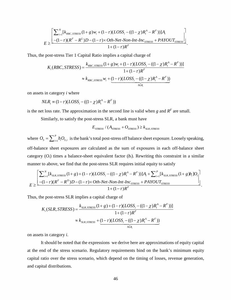
46

,1[ ( ((1(1 ) (1 ) )]

(1 )( ) (1 ) - - - -.

1 1

) )

( )

NRBC STRESS i i ii

STRESS STRESS

A Fi

F L

F

LOSS R R

R R

k g w A

D Net Non Int Inc PAYOh UR

Ot TE

χτ

τ ττ

=+ − + −

− − − − × + ≥

+ −

− −

−

∑

Thus, the post-stress Tier 1 Capital Ratio implies a capital charge of

,

,

(1 ((1 ) ))]

((1 ) )

) (1 )(( , )

1 (1 )(1 ( ))

i

RBC STRESS i ii F

RBC STRESS

A Fi

A Fi

NL

i i

R

Rk g w LOSSK RBC STRESS

Rk w LOSS

R

R R

ττ

χ

χτ

+ + −+ −

≈

− − −

+ − −−

=

−

on assets in category i where

(1 )( ((1 ) ))iA F

i iNLR S RLOS Rχτ≡ − −− −

is the net loss rate. The approximation in the second line is valid when g and RF are small.

Similarly, to satisfy the post-stress SLR, a bank must have

,/ ( )STRESS STRESS STRESS SLR STRESSE A O k+ ≥

where ,1

PS i S ii

O b O=

=∑ is the bank’s total post-stress off balance sheet exposure. Loosely speaking,

off-balance sheet exposures are calculated as the sum of exposures in each off-balance sheet

category (Oi) times a balance-sheet equivalent factor (bi). Rewriting this constraint in a similar

manner to above, we find that the post-stress SLR requires initial equity to satisfy

, ,1 1(1 ) (1 ) ] [ (1 ) ]

(1 )

[ ( ((1

( ) (1 ) - - - -.

1 ( )

) ))

1

N PSLR STRESS i i SLR STRESS i ii i

STRESS S

A F

TR

i

F D

FESS

LOSS R R

R

k g A k g b O

D Net Non Int InR Ot c Ph AYOUTE

R

χτ

τ ττ

= = + − + − − − − × + ≥

+ −

+ − − − +

−

∑ ∑

Thus, the post-stress SLR implies a capital charge of

,

,

(1 ) ( ((1 ) ))]

((1 ) )

1 )(( ,

)

)1 (1 )

(1 )(i

SLR STRESS ii F

SLR STRE

A Fi

A Fi

NLR

SS i

Rk g LOSSK SLR STRESS

RR

Rk RLOSS

τ χ

χτ

τ

+ + −+ −

≈

− − −

+ − −−

=

−

on assets in category i.

It should be noted that the expressions we derive here are approximations of equity capital

at the end of the stress scenario. Regulatory requirements bind on the bank’s minimum equity

capital ratio over the stress scenario, which depend on the timing of losses, revenue generation,

and capital distributions.

47

Empirical Implementation

Our empirical implementation is driven by a combination of data availability and a desire

for simplicity. The primary data constraint is the availability of information on interest and fee

income from different asset categories in public regulatory filings. All income statement and

balance sheet data we use come from the 2016Q4 Y-9C and Call Report regulatory filings.

For each bank and asset category, we estimate loss rates LOSSi and pretax net revenue

((1 ) )A FiR Rχ− − at the bank-category level. To approximate pretax net revenue for each bank and

category, we start by estimating the gross return on asset category i, AiR . A key data issue is that

interest and fee income is not reported in the Y-9C regulatory filings with the same granularity

that balance sheet items are. DFAST results are broken into the following categories, which can

be directly mapped to Y-9C balance sheet data: (i) first lien mortgages, (ii) junior liens and

HELOCs, (iii) commercial and industrial loans, (iv) commercial real estate loans, (v) credit card

loans, (vi) other consumer loans, and (vii) other loans.

However, income statement data is not reported with this level of granularity. Income

statement data is reported for the following categories: (i) residential mortgages, meaning loans

secured by 1-4 family residential real estate, (ii) other mortgages, (iii) commercial and industrial

loans, (iv) credit card loans, (v) other consumer loans, and (vi) Treasury securities and US

government obligations.

To make progress, we work with the categories available in the income statement data. To

estimate the gross return AiR on residential mortgages, other mortgages, and Treasury securities

and US government obligations, we divide interest and fee income over 2016, which is available

in the Y-9C filings, by matching balance sheet data on the balances for each category from the Y-

9Cs. For C&I loans, credit card loans, and other consumer loans the income statement data is

available only in the Call Reports for commercial banks. For these loan categories, we aggregate

commercial banks in the same holding company and divide interest and fee income over 2016 for

these banks by loan balances.

We then construct estimated loss rates for the same categories for which we estimate the

gross returns. DFAST reports projected losses for (i) first lien mortgages, (ii) junior liens and

HELOCs, (iii) C&I loans, (iv) commercial real estate, (v) credit card loans, (vi) other consumer

48

loans, and (vii) other loans. These loss rates are the same as those used in the CCAR, but are only

reported in the published DFAST results. We use loss rates from the severely adverse scenario.

We aggregate DFAST losses on first lien mortgages and junior liens and HELOCs, weighting by

each bank holding company’s exposure to each category, to form an estimated loss rate for our

residential mortgages category. We map DFAST losses for commercial real estate to our other

mortgages category. Finally, we assume loss rates are zero on Treasury securities and U.S.

government obligations. Total provisions projected in DFAST are the sum of loan losses and

additional changes in the allowance for loan and lease losses. Our procedure thus far includes loan

losses but not additional changes in allowances. To capture additional changes in allowances and

match total provisions in DFAST, we gross up our projected losses in each category by the ratio

of aggregate provisions in DFAST to aggregate loan losses in DFAST.

Next we allocate non-interest expense to each category. Recall that we assume that 50% of

all non-interest expenses are attributable to the lending and risk-taking activities on the asset-side

of banks’ balance sheets. To estimate the amount of non-interest expense associated with a dollar

of revenue, we divide 0.5 times non-interest expense by total interest and non-interest income at

the holding company level. The end result of this attribution procedure is to reduce each category’s

interest income by about 30% (i.e., we have 30%χ = ). We assume that FR is given by the risk-

free rate, which we proxy by the 3-month T-bill yield in the stress scenario: 10 basis points.

Given the resulting bank-category level estimates for loss rates and gross net revenue, we

aggregate up across banks to form category level estimates. We then aggregate by averaging over

banks in our sample and weighting by their loan balances in each category. Thus, our category

level estimates are estimates for the representative bank in our sample. Note that when we

aggregate we use balances from the Y-9Cs, regardless of whether our revenue estimates were

based on the Y-9Cs or the Call Reports. We have also explored other aggregations, over G-SIBs

and overall CCAR banks, and find similar results.

Note that over gross return estimates are annual, while losses are for the full 2-year stress

scenario. To match the horizon of the stress test, we multiply the quantity ((1 ) )A FiR Rχ− − by 2.

Finally, in implementing the formulas for calculating the capital charges associated with the stress

tests, we assume that both taxes and the expected growth rate of bank balance sheets in the stress

scenario are zero.

49

References

Acharya, Viral, and Sascha Steffen. 2015. “The Greatest Carry Trade Ever? Understanding Eurozone Bank Risks.” Journal of Financial Economics 115, no. 2: 215-36.

Admati, Anat R., Peter M. DeMarzo, Martin F. Hellwig, and Paul Pfleiderer. 2013. “Fallacies, Irrelevant Facts, and Myths in the Discussion of Capital Regulation: Why Bank Equity is not Socially Expensive.” Working Paper.

Avdjiev, Stefan, Patrick Bolton, Wei Jiang, and Anastasia Kartasheva. 2015. “CoCo Bond Issuance and Bank Funding Costs.” Working Paper.

Baker, Malcolm, and Jeffrey Wurgler. 2015. “Do Strict Capital Requirements Raise the Cost of Capital? Bank Regulation, Capital Structure and the Low Risk Anomaly.” American Economic Review: Papers and Proceedings 105, no. 5: 315-20.

Basel Committee on Banking Supervision. 2010. “Basel III: A Global Regulatory Framework for More Resilient Banks and Banking Systems.” December. Basel: Bank for International Settlements.

Basel Committee on Banking Supervision. 2015. “Second Consultative Document: Standards: Revisions to the Standardised Approach for Credit Risk.” Basel: Bank for International Settlements.

Behn, Markus, Rainer Haselmann, and Vikrant Vig. 2016. “The Limits of Model-Based Regulation.” European Central Bank Working Paper 1928.

Clearing House. 2017. “The Capital Allocation Inherent in the Federal Reserve’s Capital Stress Test.” Working Paper.

Cline, William R. 2017. The Right Balance for Banks: Theory and Evidence on Optimal Capital Requirements. Peterson Institute for International Economics.

Demirguc-Kunt, Asli, Enrica Detragiache, and Ourada Merrouche. 2010. “Bank Capital: Lessons from the Financial Crisis.” Working Paper no. 10/286. Washington, D.C.: International Monetary Fund.

Duffie, Darrell. 2016. “Financial Regulatory Reform After the Crisis: An Assessment.” Management Science (forthcoming).

Duffie, Darrell. 2017. “Why the Leverage Ratio Distorts Market-Making.” Risk 1.

Duffie, Darrell, and Arvind Krishnamurthy. 2016. “Passthrough Efficiency in the Fed’s New Monetary Policy Setting.” In Economic Policy Symposium Proceedings: Designing Resilient Monetary Policy Frameworks for the Future. Jackson Hole, Wyo.: Federal Reserve Bank of Kansas City.

Egan, Mark, Stefan Lewellen, and Adi Sunderam. 2017. “The Cross Section of Bank Value.” Working Paper.

50

Estrella, Arturo, Sangkyun Park, and Stavros Peristiani. 2000. “Capital Ratios as Predictors of Bank Failure.” Economic Policy Review 6, no. 2: 33-52.

Federal Deposit Insurance Corporation. 1997. “Banking Legislation and Regulation.” Chapter 2 of History of the Eighties: Lessons for the Future.

Federal Reserve Bank of Minneapolis. 2016. “The Minneapolis Plan to End Too Big to Fail.” December.

Federal Reserve Board of Governors. 2015. “Calibrating the G-SIB Surcharge.” White Paper, July 20.

Firestone, Simon, Amy Lorenc, and Ben Ranish. 2017. “An Empirical Economic Assessment of the Costs and Benefits of Bank Capital in the U.S.” Finance and Economics Discussion Series 2017-034. Washington: Board of Governors of the Federal Reserve System.

Flannery, Mark, Beverly Hirtle, and Anna Kovner. 2017. “Evaluating the Information in the Federal Reserve Stress Tests.” Journal of Financial Intermediation 29, 1-18.

Goldstein, Morris. 2017. Banking’s Final Exam: Stress Testing and Bank-Capital Reform. Peterson Institute for International Economics.

Goodhart, Charles. 1975. “Problems of Monetary Management: The U.K. Experience.” In Monetary Theory and Practice. London: Palgrave.

Gorton, Gary B. 2010. Slapped by the Invisible Hand: The Panic of 2007. London: Oxford University Press.

Gorton, Gary B., and Andrew Metrick. 2012. “Securitized Banking and the Run on Repo.” Journal of Financial Economics 104, no. 3: 425-451.

Greenwald, Bruce, Joseph E. Stiglitz and Andrew Weiss. 1984. “Informational Imperfections in the Capital Market and Macroeconomic Fluctuations.” American Economic Review 74:194−199.

Greenwood, Robin, Samuel G. Hanson, and Jeremy C. Stein. 2015. “A Comparative-Advantage Approach to Government Debt Maturity.” Journal of Finance 70, no. 4: 1683-722.

Greenwood, Robin, Samuel G. Hanson, Jeremy C. Stein, and Adi Sunderam. 2017. “The Financial Regulatory Reform Agenda in 2017.” Working Paper.

Haldane, Andrew, and Vasileios Madouros. 2012. “The Dog and the Frisbee.” In Economic Policy Symposium Proceedings: The Changing Policy Landscape. Jackson Hole, Wyo.: Federal Reserve Bank of Kansas City.

Hanson, Samuel G., Anil Kashyap, and Jeremy C. Stein. 2011. “A Macroprudential Approach to Financial Regulation.” Journal of Economic Perspectives 25, no. 1: 3-28.

Hanson, Samuel G., Andrei Shleifer, Jeremy C. Stein, and Robert Vishny. 2015. “Banks as Patient Fixed Income Investors.” Journal of Financial Economics 117, no. 3: 449-469.

Kashyap, Anil, and Jeremy C. Stein. 2004. “Cyclical Implications of the Basel II Capital Standards.” Federal Reserve Bank of Chicago Economic Perspectives 28, Q1: 18-31

51

Krishnamurthy, Arvind, and Annette Vissing-Jorgensen. 2012. “The Aggregate Demand for Treasury Debt.” Journal of Political Economy 120: 233-267

Krishnamurthy, Arvind, and Annette Vissing-Jorgensen. 2016. “The Impact of Treasury Supply on Financial Sector Lending and Stability.” Journal of Financial Economics 118, no. 3: 571-600.

Liang, Nellie. 2017a. “Financial Regulations and Macroeconomic Stability.” Keynote Address at the International Finance and Banking Society, July 15-17, Said Business School, Oxford.

Liang, Nellie. 2017b. “Higher Capital is not a Substitute for Stress Tests.” April 24. Washington: The Brookings Institution Report.

Lucas, Robert E., Jr. 1976. “Econometric Policy Evaluation: A Critique.” In: K. Brunner and A. Meltzer (eds.), The Phillips Curve and Labor Markets, Carnegie-Rochester Conference Series on Public Policy, Vol. 1: 19-46.

Modigliani, Franco, and Merton H. Miller. 1958. “The Cost of Capital, Corporation Finance, and the Theory of Investment.” American Economic Review 48, no. 3: 261-297.

Myers, Stewart. 1977. “Determinants of Corporate Borrowing.” Journal of Financial Economics 5, no. 2: 147-75.

Myers, Stewart, and Nicholas Majluf. 1984. “Corporate Financing and Investment Decisions When Firms Have Information That Investors Do Not Have.” Journal of Financial Economics 13, no. 2: 187-221.

Passmore, Wayne, and Alexander H. von Hafften. 2017. “Are Basel’s Capital Surcharges For Global Systemically Important Banks Too Small?” Finance and Economics Discussion Series 2017-021. Washington: Board of Governors of the Federal Reserve System.

Sarin, Natasha, and Lawrence H. Summers. 2016. “Understanding Bank Risk through Market Measures.” Brookings Papers on Economic Activity, Fall 2016: 57-109.

Stein, Jeremy C. 2012. “Monetary Policy as Financial-Stability Regulation.” Quarterly Journal of Economics 127, no. 1: 57-95.

Stein, Jeremy C. 2013. “Lean, Clean, and In-Between.” Speech given at the National Bureau of Economic Research Conference: Lessons from the Financial Crisis for Monetary Policy, Boston, Massachusetts, October 18.

Sunderam, Adi. 2015. “Money Creation and the Shadow Banking System.” Review of Financial Studies, 28, no. 4: 939-77.

Tarullo, Daniel K. 2017. “Departing Thoughts.” Speech given at the Woodrow Wilson School, Princeton University, Princeton, NJ, April 4.

Wall, L.D. 1989. “Capital Requirements for Banks: A Look at the 1981 and 1988 Standards.” Federal Reserve Bank of Atlanta Economic Review, March/April, 14-29.

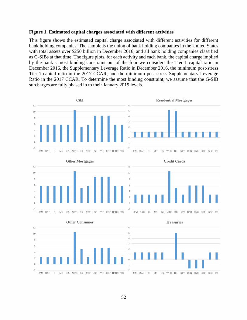
52

Figure 1. Estimated capital charges associated with different activities

This figure shows the estimated capital charge associated with different activities for different bank holding companies. The sample is the union of bank holding companies in the United States with total assets over $250 billion in December 2016, and all bank holding companies classified as G-SIBs at that time. The figure plots, for each activity and each bank, the capital charge implied by the bank’s most binding constraint out of the four we consider: the Tier 1 capital ratio in December 2016, the Supplementary Leverage Ratio in December 2016, the minimum post-stress Tier 1 capital ratio in the 2017 CCAR, and the minimum post-stress Supplementary Leverage Ratio in the 2017 CCAR. To determine the most binding constraint, we assume that the G-SIB surcharges are fully phased in to their January 2019 levels.

-2

0

2

4

6

8

10

12

JPM BAC C MS GS WFC BK STT USB PNC COF HSBC TD

C&I

-2

-1

0

1

2

3

4

5

6

JPM BAC C MS GS WFC BK STT USB PNC COF HSBC TD

Residential Mortgages

-2

0

2

4

6

8

10

12

JPM BAC C MS GS WFC BK STT USB PNC COF HSBC TD

Other Mortgages

-2

0

2

4

6

8

10

12

JPM BAC C MS GS WFC BK STT USB PNC COF HSBC TD

Credit Cards

-2

0

2

4

6

8

10

12

JPM BAC C MS GS WFC BK STT USB PNC COF HSBC TD

Other Consumer

-2

-1

0

1

2

3

4

5

6

JPM BAC C MS GS WFC BK STT USB PNC COF HSBC TD

Treasuries

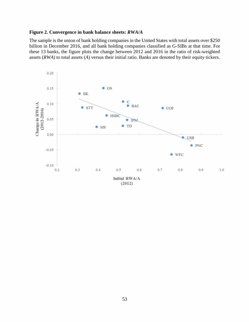
53

Figure 2. Convergence in bank balance sheets: RWA/A

The sample is the union of bank holding companies in the United States with total assets over $250 billion in December 2016, and all bank holding companies classified as G-SIBs at that time. For these 13 banks, the figure plots the change between 2012 and 2016 in the ratio of risk-weighted assets (RWA) to total assets (A) versus their initial ratio. Banks are denoted by their equity tickers.

54

Table 1. Distance from different capital requirements

The first panel shows required capital ratios (in percentage points) by bank for G-SIBs and banks with more than $250 billion in assets in December 2016. The second panel shows actual capital ratios taken from December 2016 Y9-C filings (Tier 1 ratio and SLR) and results of the 2017 Comprehensive Capital Analysis and Review (CCAR). The third panel lists the difference between required and actual ratios expressed in percentage points. In the third panel, the most binding constraint is shown in bold. To determine the most binding constraint, we assume that the G-SIB surcharges are fully phased in to their January 2019 levels.

Required ratios (%) Actual 2016Q4 ratios (%) Distance from Requirement (%)

Tier 1 Ratio SLR

CCAR Tier 1 Ratio

CCAR SLR

Tier 1 Ratio SLR

CCAR Tier 1 Ratio

CCAR SLR

Tier 1 Ratio SLR

CCAR Tier 1 Ratio

CCAR SLR

G-SIBs: JPMorgan Chase 12.0 5.0 6.0 3.0 14.2 6.5 8.4 3.9 2.2 1.5 2.4 0.9 Bank of America 11.5 5.0 6.0 3.0 13.6 7.0 8.4 4.3 2.1 2.0 2.4 1.3 Citigroup Inc. 11.5 5.0 6.0 3.0 15.8 7.6 9.5 4.5 4.3 2.6 3.5 1.5 Morgan Stanley 11.5 5.0 6.0 3.0 20.0 6.4 10.3 3.2 8.5 1.4 4.3 0.2 Goldman Sachs 11.0 5.0 6.0 3.0 16.6 6.5 8.2 3.1 5.6 1.5 2.2 0.1 Wells Fargo 10.5 5.0 6.0 3.0 12.8 7.6 9.0 5.3 2.3 2.6 3.0 2.3 Bank of New York Mellon 10.0 5.0 6.0 3.0 14.5 6.0 11.6 4.8 4.5 1.0 5.6 1.8 State Street 10.0 5.0 6.0 3.0 14.7 5.9 9.1 3.6 4.7 0.9 3.1 0.6 Other Large BHCs: U.S. Bancorp 8.5 3.0 6.0 3.0 11.0 7.3 7.9 5.2 2.5 4.3 1.9 2.2 PNC Financial Services 8.5 3.0 6.0 3.0 12.0 8.6 7.6 5.4 3.5 5.6 1.6 2.4 Capital One Financial 8.5 3.0 6.0 3.0 11.6 8.5 7.1 5.4 3.1 5.5 1.1 2.4 HSBC North America 8.5 3.0 6.0 3.0 20.1 7.3 11.6 4.0 11.6 4.3 5.6 1.0 TD Group US 8.5 3.0 6.0 3.0 13.7 7.1 11.3 5.8 5.2 4.1 5.3 2.8

55

Table 2. Assumptions on risk weights, losses, and net revenue by activity This table reports the assumptions that underlie our estimated capital charges. We report risk weights from the U.S. implementation of the Basel II Standardized Approach. Assumed losses (𝑁𝑁𝐶𝐶𝐶𝐶𝐶𝐶𝑖𝑖 ) are 2-year loss projections from severely adverse scenario of the 2017 Dodd-Frank-Act supervisory stress tests conducted by the Federal Reserve. We compute the average loss rate for the 13 BHCs in our sample weighted by each bank’s loan balances in the asset category. The reported loss rates are “grossed up” by approximately 10% to ensure that total losses equal total provisions in the severely adverse stress scenario. Gross interest and fee income (𝑅𝑅𝑖𝑖𝐴𝐴 ) for each loan category are averages for the 13 BHCs over 2016, again weighted by each bank's loan balances in each category. The contribution to PPNR for each loan category ((1 − 𝜒𝜒)𝑅𝑅𝑖𝑖𝐴𝐴 − 𝑅𝑅𝐹𝐹) subtracts off a non-interest expense charge (we assume 𝜒𝜒 = 30%) and the wholesale funding rate (assumed to be 𝑅𝑅𝐹𝐹 = 0.1%, the 3-month Treasury bill yield projected in the severely adverse scenario). The 2-year net loss rate is then given by 𝑁𝑁𝑁𝑁𝑅𝑅𝑖𝑖 = 𝑁𝑁𝐶𝐶𝐶𝐶𝐶𝐶𝑖𝑖 − 2 × ((1 − 𝜒𝜒)𝑅𝑅𝑖𝑖𝐴𝐴 − 𝑅𝑅𝐹𝐹 ) .

C&I Residential Mortgages

Other Mortgages

Credit Cards

Other Consumer Treasuries

Risk weight (𝑤𝑤𝑖𝑖) 100 50 100 100 100 0

𝑁𝑁𝐶𝐶𝐶𝐶𝐶𝐶𝑖𝑖 (2-year rate) 7.3 3.3 7.3 15.8 5.6 0.0

𝑅𝑅𝑖𝑖𝐴𝐴 (1-year rate) 3.4 3.8 3.5 11.5 4.6 1.3

(1 − 𝜒𝜒)𝑅𝑅𝑖𝑖𝐴𝐴 − 𝑅𝑅𝐹𝐹 (1-year rate) 2.3 2.6 2.3 8.0 3.1 0.8

𝑁𝑁𝑁𝑁𝑅𝑅𝑖𝑖 (2-year rate) 2.7 -1.9 2.7 -0.2 -0.6 -1.7

56

Table 3. Estimated capital charges under different capital requirements This table reports our estimated capital charges under different capital requirements. The capital charge is the incremental amount of equity that a constrained bank must have for an incremental dollar of lending in loan category i. In the second row, we assume the G-SIB surcharge takes its highest current value (3.5%) and is fully phased in.

C&I Residential Mortgages

Other Mortgages

Credit Cards

Other Consumer Treasuries

Tier 1 Ratio (non G-SIB) 8.5 4.3 8.5 8.5 8.5 0.0

Tier 1 Ratio (highest G-SIB) 12.0 6.0 12.0 12.0 12.0 0.0

SLR (non G-SIB) 3.0 3.0 3.0 3.0 3.0 3.0

SLR (G-SIB) 5.0 5.0 5.0 5.0 5.0 5.0

CCAR Tier 1 Ratio 8.7 1.1 8.7 5.8 5.4 -1.7

CCAR SLR 5.7 1.1 5.7 2.8 2.4 1.3

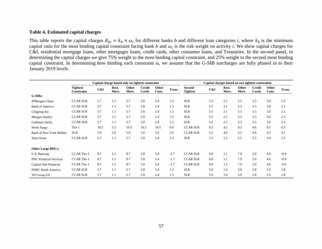
57

Table 4. Estimated capital charges

This table reports the capital charges 𝐾𝐾𝑏𝑏𝑖𝑖 = 𝑘𝑘𝑏𝑏 × 𝜔𝜔𝑖𝑖 for different banks b and different loan categories i, where 𝑘𝑘𝑏𝑏 is the minimum capital ratio for the most binding capital constraint facing bank b and 𝜔𝜔𝑖𝑖 is the risk weight on activity i. We show capital charges for C&I, residential mortgage loans, other mortgages loans, credit cards, other consumer loans, and Treasuries. In the second panel, in determining the capital charges we give 75% weight to the most binding capital constraint, and 25% weight to the second most binding capital constraint. In determining how binding each constraint is, we assume that the G-SIB surcharges are fully phased in to their January 2019 levels.

Capital charge based only on tightest constraint Capital charges based on two tightest constraints

Tightest Constraint C&I Resi.

Mort. Other Mort.

Credit Cards

Other Cons. Treas. Second

Tightest C&I Resi. Mort.

Other Mort.

Credit Cards

Other Cons. Treas.

G-SIBs: JPMorgan Chase CCAR SLR 5.7 1.1 5.7 2.8 2.4 1.3 SLR 5.5 2.1 5.5 3.3 3.0 2.3

Bank of America CCAR SLR 5.7 1.1 5.7 2.8 2.4 1.3 SLR 5.5 2.1 5.5 3.3 3.0 2.3

Citigroup Inc. CCAR SLR 5.7 1.1 5.7 2.8 2.4 1.3 SLR 5.5 2.1 5.5 3.3 3.0 2.3

Morgan Stanley CCAR SLR 5.7 1.1 5.7 2.8 2.4 1.3 SLR 5.5 2.1 5.5 3.3 3.0 2.3

Goldman Sachs CCAR SLR 5.7 1.1 5.7 2.8 2.4 1.3 SLR 5.5 2.1 5.5 3.3 3.0 2.3

Wells Fargo Tier 1 10.5 5.3 10.5 10.5 10.5 0.0 CCAR SLR 9.3 4.2 9.3 8.6 8.5 0.3

Bank of New York Mellon SLR 5.0 5.0 5.0 5.0 5.0 5.0 CCAR SLR 5.2 4.0 5.2 4.4 4.3 4.1

State Street CCAR SLR 5.7 1.1 5.7 2.8 2.4 1.3 SLR 5.5 2.1 5.5 3.3 3.0 2.3

Other Large BHCs:

U.S. Bancorp CCAR Tier 1 8.7 1.1 8.7 5.8 5.4 -1.7 CCAR SLR 8.0 1.1 7.9 5.0 4.6 -0.9

PNC Financial Services CCAR Tier 1 8.7 1.1 8.7 5.8 5.4 -1.7 CCAR SLR 8.0 1.1 7.9 5.0 4.6 -0.9

Capital One Financial CCAR Tier 1 8.7 1.1 8.7 5.8 5.4 -1.7 CCAR SLR 8.0 1.1 7.9 5.0 4.6 -0.9

HSBC North America CCAR SLR 5.7 1.1 5.7 2.8 2.4 1.3 SLR 5.0 1.6 5.0 2.8 2.5 1.8

TD Group US CCAR SLR 5.7 1.1 5.7 2.8 2.4 1.3 SLR 5.0 1.6 5.0 2.8 2.5 1.8

58

Table 5. Estimate relative risk weights

In this table, we convert the estimated capital charges in Table 4 to effective risk weights for each activity and each bank. Specifically, for each bank we rescale each capital charge by the bank’s capital charge for C&I lending, which receives a risk weight of 100% in the U.S. implementation of the Basel II Standardized Approach. We first show such risk weights based on only the tightest constraint for each bank. The second panel shows risk weights based on the two tightest constraints for each bank, where the tightest constraint receives 75% weight and the next tightest constraints receives 25% weight. In determining how binding each constraint is, we assume that the G-SIB surcharges are fully phased in to their January 2019 levels.

Effective risk weight based only on tightest constraint Effective risk weight based on two tightest constraints

Tightest Constraint C&I Resi.

Mort. Other Mort.

Credit Cards

Other Cons. Treas. Second

Tightest C&I Resi. Mort.

Other Mort.

Credit Cards

Other Cons. Treas.

G-SIBs: JPMorgan Chase CCAR SLR 100 19 99 49 42 23 SLR 100 38 99 61 55 41

Bank of America CCAR SLR 100 19 99 49 42 23 SLR 100 38 99 61 55 41

Citigroup Inc. CCAR SLR 100 19 99 49 42 23 SLR 100 38 99 61 55 41

Morgan Stanley CCAR SLR 100 19 99 49 42 23 SLR 100 38 99 61 55 41

Goldman Sachs CCAR SLR 100 19 99 49 42 23 SLR 100 38 99 61 55 41

Wells Fargo Tier 1 100 50 100 100 100 0 CCAR SLR 100 45 100 92 91 4

Bank of New York Mellon SLR 100 100 100 100 100 100 CCAR SLR 100 78 100 86 84 79

State Street CCAR SLR 100 19 99 49 42 23 SLR 100 38 99 61 55 41

Other Large BHCs:

U.S. Bancorp CCAR Tier 1 100 13 100 67 62 -19 CCAR SLR 100 14 99 63 58 -11

PNC Financial Services CCAR Tier 1 100 13 100 67 62 -19 CCAR SLR 100 14 99 63 58 -11

Capital One Financial CCAR Tier 1 100 13 100 67 62 -19 CCAR SLR 100 14 99 63 58 -11

HSBC North America CCAR SLR 100 19 99 49 42 23 SLR 100 31 99 57 50 35

TD Group US CCAR SLR 100 19 99 49 42 23 SLR 100 31 99 57 50 35