HAL Id: hal-01789422https://hal.archives-ouvertes.fr/hal-01789422

Submitted on 10 May 2018

HAL is a multi-disciplinary open accessarchive for the deposit and dissemination of sci-entific research documents, whether they are pub-lished or not. The documents may come fromteaching and research institutions in France orabroad, or from public or private research centers.

L’archive ouverte pluridisciplinaire HAL, estdestinée au dépôt et à la diffusion de documentsscientifiques de niveau recherche, publiés ou non,émanant des établissements d’enseignement et derecherche français ou étrangers, des laboratoirespublics ou privés.

Streamline simulation of water-oil displacement in aheterogeneous fractured reservoir using different

transfer functionsMohammad Mesbah, Ali Vatani, Majid Siavashi

To cite this version:Mohammad Mesbah, Ali Vatani, Majid Siavashi. Streamline simulation of water-oil displacementin a heterogeneous fractured reservoir using different transfer functions. Oil & Gas Science andTechnology - Revue d’IFP Energies nouvelles, Institut Français du Pétrole (IFP), 2018, 73, pp.14.�10.2516/ogst/2018004�. �hal-01789422�

Oil & Gas Science and Technology - Rev. IFP Energies nouvelles 73, 14 (2018)© M. Mesbah et al., published by IFP Energies nouvelles, 2018https://doi.org/10.2516/ogst/2018004

Available online at:www.ogst.ifpenergiesnouvelles.fr

REGULAR ARTICLE

Streamline simulation of water-oil displacement in aheterogeneous fractured reservoir using different transferfunctionsMohammad Mesbah1, Ali Vatani2,*, and Majid Siavashi3

1 PhD Candidate of Petroleum Engineering, School of Chemical Engineering, Institute of Petroleum Engineering, University ofTehran, Tehran, Iran

2 Professor of Chemical Engineering, Institute of LNG, College of Engineering, University of Tehran, Tehran, Iran3 Assistant professor of Mechanical Engineering, Applied Multi-Phase Fluid Dynamics Laboratory, School of MechanicalEngineering, Iran University of Science and Technology, Tehran, Iran

* Correspo

This is an O

Received: 17 November 2017 / Accepted: 1 February 2018

Abstract. Main parts of oil and gas reserves are stored in fractured reservoirs. Simulation of multiphase flow infractured reservoirs requires a large amount of calculations due to the complexity, reservoir scale andheterogeneityof the rock properties. The accuracy and speed of the streamline method for simulating hydrocarbon reservoirs atfield scale make it more applicable than conventional Eulerian simulators using finite difference and finite elementtechniques. Conventional simulators for fractured reservoirs consume a great deal of time and expense and requirepowerfulCPUs like supercomputers.Thismakes thedevelopmentof a fast,powerful andprecise simulationmethodofgreat importance.Thepresentstudywasundertakentodevelopacomputationalcodeasastreamlinesimulatortostudy waterflooding in a two-dimensional fractured reservoir with heterogeneous permeability using the DualPorosity-Single Permeability (DPSP) model. In this simulator, the pressure equation is solved implicitly over anEulerian grid and then the streamlines are generatedusingPollock’s semi-analyticalmethodand are traced.At thispoint, theTime-Of-Flight (TOF) is developed and the saturation equations aremappedand solved explicitly alongthe streamlines.Next, the results are transferred back onto theEuleriangrid and the calculations are repeateduntilthe simulation end time. In fractured reservoirs, the interaction between the matrix and fracture is included in thetransfer functions. Transfer functions model fluid flow and production mechanisms between the matrix andfracture. They introduce source/sink equations between the matrix and fracture and they are distributedthroughout themedia. In the current study, a problem is simulated using streamlinemethodand several importanttransfer functions. A new linear transfer function with a constant coefficient is introduced that is based ondifferences in water saturation between thematrix and fracture. The simulation results were then compared and acommercial software is applied to solve the same problem. The results of the streamline simulator were comparedwith those of the commercial software and showedappropriate accuracy for thenewly introduced transfer function.Theaccuracyandefficiencyof the streamline simulator for simulationoftwo-phaseflowin fracturedreservoirsusingdifferent transfer functions are confirmed and the results are verified.

1 Introduction

Simulation offluidflow in porousmedia in order to improveoil production from hydrocarbon reservoirs is vital. Thisincludes proposing a Master Development Planning(MDP) for reservoir management (Siavashi et al., 2014).

Most countries that have a large oil and gas reserves areconcerned with fractured reservoirs (Bourbiaux, 2010).Fractured porous media are characterized by substantial

nding author: avatani@ut.ac.ir

pen Access article distributed under the terms of the Creative Comwhich permits unrestricted use, distribution, and reproduction

differences in the properties of the matrix and fractureregions (Noetinger et al., 2016). Recent research has shownthat the ultimate recovery factor for a fractured reservoir is<10–60% or 70% (Bourbiaux, 2010). Simulation as amethod of predicting fluid behavior using conventionalsimulators and the Eulerian approach is time-consumingand requires strong computing hardware (Biagi et al.,2016). Achieving an appropriate simulation method isessential. The streamline method is a powerful methodwith advantages and useful applications over conventionalsimulation methods based on finite volume and finitedifference approaches. The streamline technique can be

mons Attribution License (http://creativecommons.org/licenses/by/4.0),in any medium, provided the original work is properly cited.

Fig. 1. Schematics of different fracture � models for simulatingfractured reservoirs (Datta-Gupta and King, 2007).

2 M. Mesbah et al.: Oil & Gas Science and Technology - Rev. IFP Energies nouvelles 73, 14 (2018)

used to simulate hydrocarbon reservoirs at field scale withappropriate speed and accuracy (Batycky et al., 1997). Inaddition to its speed and precision, it has advantages whichprovide better flow visualization patterns and wellintercommunication.

Fractured reservoirs can be divided into two connectedmedia; the fracture network that provides the main path forfluid flow and matrix blocks, which are porous media andprovide the bulk of reservoir volume and storage capacity.Three-dimensional images of fracture networks obtained byfield fracturing data integration and stochastic modelingare highly complex and cannot be applied as direct input fora reservoir simulator (Bourbiaux et al., 1998). When fluidflow in reservoirs is simulated using mathematical models,the average properties of the porous media are used.

There are three general types of fractured reservoirs(Bourbiaux, 2010):

Type A has a very tight matrix; thus, fluid flow andstorage are not feasible in the matrix section. Thepermeability and porosity of the reservoir are determinedby the fracture section (Single-Porosity Single-Permeabil-ity model (SPSP)). In type B, the matrix section hasgreater storage capacity for fluids and determines the mainporosity of reservoir. The fluid flow rate is low in thematrix, and the matrix does not make a large contributionto the overall permeability of the reservoir (Dual-PorositySingle-Permeability (DPSP) model). In type C, the matrixsection is porous and permeable and has an effectivepermeability similar to that of the fracture section (Dual-Porosity Dual-Permeability (DPDP) model).

The use of the SPSP, DPSP and DPDP models forsimulation of fractured reservoirs are summarized inFigure 1 (Barenblatt et al., 1960; Di Donato et al., 2003;Datta-Gupta and King, 2007).

The DPSP model was used in this research because thepermeability of matrix was considered to be small enoughto ignore the Darcy flow (Jerbi et al., 2017). This modelrepresents the matrix blocks as the source of the fracturenetwork and fluid only flows in the fractures. This theory isreasonable because of the high-speed fluid flow in thefracture network with respect to the matrix blocks; thus,the fluid flow between the matrix blocks is neglected(Gilman, 2003).

A major challenge to simulating fractured reservoirs isthe limited computing capacity of conventional simulators(Bourbiaux, 2010). The streamline method was derivedfrom the streamtube method (LeBlanc and Caudle, 1971);however, the streamtube method has major problems andlimitations. For example, changes in the rate and locationof wells were not possible and, in most cases, the effect ofgravity is ignored. The introduction and development ofthe streamlines concept solved many of these limitations(Baker, 2001).

Conventional simulation techniques based on the finitedifference method have a two-step solution. In the firststep, the pressure equation is solved and the pressuredistribution in the domain is calculated. In the second step,the saturation equation is solved. In the streamlinemethod, as in the IMplicit Pressure-Explicit Saturation(IMPES) reservoir simulation method, the pressuredistribution is obtained implicitly over the Eulerian grid

and then the streamlines are drawn using Pollock’s semi-analytical method. Afterwards, the transport equations aresolved explicitly and linearly along the streamlines.Because the equations are one-dimensional along thestreamlines, the number of calculations and, therefore, theamount of memory required for simulation is less than forconventional methods.

In conventional simulation methods, fluid flowsbetween the simulation cells. In the streamline method,fluid flows in the direction of the pressure difference,which coincides with the physics of flow. The streamlinemethod has two different timesteps. The total timestep(Dttotal) is used to solve the pressure equation implicitly.The local timestep (Dtsl), or streamlines timestep, is usedto solve the saturation equation explicitly along thestreamlines. The implicit solution has no stabilitylimitations in comparison with the explicit method whenusing large timesteps. Therefore, a larger total timestepsize can be chosen to reduce the number of pressuresolution updates and increase the simulation speed.These two timesteps are shown in Figure 2 (Doranehgardand Siavashi, 2018).

The increase in the speed of streamline method derivesmainly from avoidance of the updating of the pressure fieldaccording to changes in the level of saturation. Anotherfactor that increases the simulation speed is that everystreamline is calculated separately, independent of otherstreamlines, with its own timestep size (Dtsl).

The non-linear transport equations make the finitedifference method very sensitive to changes in the size andorientation of the simulation cells and timestep (Baker,2001). The streamline method is, therefore, more stable(Batycky et al., 1997). The streamlines never cross eachother; thus, the amount of fluid produced is the sum of thestreamlines (Siavashi et al., 2016). The merits of streamlinemethod are as follows:

–

high calculation speed and high accuracy; – appropriate visualization of fluid flow and the relation-ship between the production and injection wells;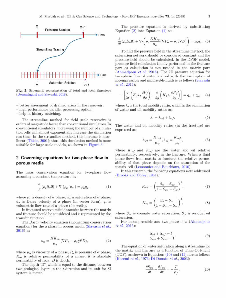

Fig. 2. Schematic representation of total and local timesteps(Doranehgard and Siavashi, 2018).

M. Mesbah et al.: Oil & Gas Science and Technology - Rev. IFP Energies nouvelles 73, 14 (2018) 3

–

better assessment of drained areas in the reservoir; – high performance parallel processing option; – help in history-matching.

The streamline method for field scale reservoirs isorders of magnitude faster than conventional simulators. Inconventional simulators, increasing the number of simula-tion cells will almost exponentially increase the simulationrun time. In the streamline method, this increase is near-linear (Thiele, 2001); thus, this simulation method is moresuitable for large scale models, as shown in Figure 3.

2 Governing equations for two-phase flow inporous media

The mass conservation equation for two-phase flowassuming a constant temperature is:

∂∂tðraSa∅Þ þ ∇⋅ðra ua Þ ¼ raqa; ð1Þ

where ra is density of a phase, Sa is saturation of a phase,~u∝ is Darcy velocity of a phase (in vector form), qa isvolumetric flow rate of a phase (for wells).

In fractured reservoirs fluid transfer between thematrixand fracture should be considered and is represented by thetransfer function.

The Darcy velocity equation (momentum conservationequation) for the a phase in porous media (Siavashi et al.,2016) is:

ua ¼ KKra

ma

ð∇Pa � rag∇DÞ; ð2Þ

where ma is viscosity of a phase, Pa is pressure of a phase,Kra is relative permeability of a phase, K is absolutepermeability of rock, D is depth.

The depth “D”, which is equal to the distance betweentwo geological layers in the z-direction and its unit for SIsystem is meter.

The pressure equation is derived by substitutingEquation (2) into Equation (1) as:

∂∂t

ðraSa∅Þ þ ∇⋅ raKKra

ma

ð∇Pa � rag∇DÞ� �

¼ raqa: ð3Þ

To find the pressure field in the streamline method, thesaturation network should be considered constant and thepressure field should be calculated. In the DPSP model,pressure field calculation is only performed in the fracturepart as calculation is not needed in the matrix part(Ahmadpour et al., 2016). The 2D pressure equation fortwo-phase flow of water and oil with the assumption ofincompressible and immiscible fluids is as follows (Siavashiet al., 2014):

� ∂∂x

Kflt∂Pf

∂x

� �þ ∂∂y

Kflt∂Pf

∂y

� �� �¼ qw þ qo; ð4Þ

where lt is the total mobility ratio, which is the summationof water and oil mobility ratios as:

lt ¼ lwf þ lof : ð5ÞThe water and oil mobility ratios (in the fracture) areexpressed as:

lwf ¼ Krwf

mw

; lof ¼ Krof

mo

; ð6Þ

where Krwf and Krof are the water and oil relativepermeability, respectively, in the fracture. When a fluidphase flows from matrix to fracture, the relative perme-ability of that phase depends on the saturation of thematrix cell (Lemonnier and Bourbiaux, 2010).

In this research, the following equations were addressed(Brooks and Corey, 1964):

Krw ¼ Sw � Swc

1� Swc � Sor

� �2

; ð7Þ

Kro ¼ So � Sor

1� Swc � Sor

� �2

; ð8Þ

where Swc is connate water saturation, Sor is residual oilsaturation.

For incompressible and two-phase flow (Ahmadpouret al., 2016):

Sof þ Swf ¼ 1Som þ Swm ¼ 1

: ð9Þ

The equation of water saturation along a streamline forthe matrix and fracture as a function of Time-Of-Flight(TOF), as shown in Equations (10) and (11), are as follows(Kazemi et al., 1976; Di Donato et al., 2003):

∂Swf

∂tþ ∂fwf

∂t¼ � T

’f

; ð10Þ

Fig. 3. Simulation run time ratio for various number of grids forstreamline and conventional (IMPES) method.

4 M. Mesbah et al.: Oil & Gas Science and Technology - Rev. IFP Energies nouvelles 73, 14 (2018)

∂Swm

∂t¼ T

’m

: ð11Þ

TOF (t) (Batycky et al., 1997) is defined as the timerequired for a particle to travel distance S along astreamline traced from a source (e.g. an injection well)to a sink (e.g. a production well) and is written as (Siavashiet al., 2016):

t ¼ ∫s

0

’

j~u ðdÞjdd; ð12Þ

where ’ is the porosity and d and ~u are the location andvelocity of the particle along the streamlines, respectively.

This component separates the effects of geologicalheterogeneity from the transport equations (mass andmomentum) and converts the 3D physical coordinates tomultiple 1D TOF coordinates, allowing the transportequations to be solved simply. This is done by mapping thesaturation equations from the 3D coordinates to the TOFcoordinates. The multi-dimensional saturation equationsare converted to a series of 1D equations for calculatingvariations in saturation along the streamlines. In addition,because only one streamline is loaded in the memory at anymoment, the amount of memory required to perform thesimulation is reduced significantly.

In Equation (10), fwf is the fractional flow of water in thefracture:

fwf ¼lwf

lwf þ lof: ð13Þ

The general steps of streamline simulation for afractured reservoir using the DPSP model are as follows(Datta-Gupta and King, 2007; Hassane, 2013):

1) By using the numerical solution for the pressureequation and application of the Darcy law, the pressuredistribution and fluid velocity for the fracture at one totaltimestep are achieved for the initial condition (for pressure

and irreducible water saturation), porosity, permeabilitydistribution and well and boundary conditions(Vitoonkijvanich et al., 2015).

2) The streamlines are drawn using Pollock’s method(Pollock, 1988) considering the fluid velocity distributionin the fracture. It is assumed that the only connectionbetween the injection and production wells is the fracturenetwork because of the high fluid velocity of the fracture incomparison with the matrix.

3) When the streamlines are drawn, the TOF alongthem is calculated. The TOF contour locates and predictsthe injected fluid front at the selected reservoir atdifferent times and is a major advantage of the streamlinemethod.

4) Fluid saturation and other fluid characteristics aretransposed from solution grids to the streamlines. Bysolving the transport equations, fluid saturation can becalculated in matrix and fracture (Di Donato and Blunt,2004). The transport equations are solved using a 1Dtechnique along the streamlines in terms of TOF. In thestreamline method, the explicit solution for the transportequations requires the use of a local timestep (Dtsl) that issmaller than the total timestep (Dttotal) (Choobineh et al.,2015).

5) After solving the equations in a total timestep, thefluid saturation is transposed from the streamlines to thesolution grids. A source of error in the streamline methodoccurs when transporting the solutions (fluid saturations)from the Eulerian grid to the streamlines and vice versa.

6) The operator-splitting technique is used for anyeffects running in different directions than the streamlines,such as the effect of gravity (Siavashi et al., 2014).

7) Repeat the previous steps until the simulation ends.

3 Matrix-fracture transfer functions

Transfer function defined as it specifically characterizesfractured reservoir flow behavior. From the dual porosityperspective, the fracturemediumandthematrixmediumactas flow regions in which themedia interact. This interactionis defined mathematically by means of matrix-fracturetransfer functions. The effect of the matrix-fracture mecha-nisms can differ and include variability of the flowpropertiesin the matrix porous medium and the characteristics of thefracture network (Lemonnier and Bourbiaux, 2010).

Several transfer functions for simulation of fracturedreservoirs using dual porosity are discussed below. In thesetransfer functions, the effects of gravity and compressibili-ty are neglected and fluid transfer between the matrix andfracture is controlled by imbibition process. The imbibitionprocess plays a vital role in matrix-fracture fluid transfer(Sarma and Aziz, 2004).

3.1 Conventional transfer function (Kazemi et al.,1976)

The interaction (fluid transportation) between the matrixand fracture in the DPSP model is represented by thetransfer functions (Ti). Kazemi et al. (1976) introduced the

M. Mesbah et al.: Oil & Gas Science and Technology - Rev. IFP Energies nouvelles 73, 14 (2018) 5

first multi-phase transfer function, known as the conven-tional transfer function, which is most commonly used infractured reservoir simulation and many commercialsimulator software packages (Gilman and Kazemi, 1983;Di Donato et al., 2003). They defined capillary pressure tointroduce a transfer function that confirms the experimen-tal results (Di Donato and Blunt, 2004).

The simplified form of this transfer function thatconsiders 2DDarcy flow (Gilman andKazemi, 1983; Datta-Gupta and King, 2007) can be written as:

Tw ¼ FsKmlwfðPwf � PwmÞTo ¼ FsKmlofðPof � PomÞ ; ð14Þ

where Fs is the shape factor.These two equations are functions of the matrix and

fracture phase saturation and pressure. The exchange ratebetween the matrix and fracture depends on the size of thematrix block. It considers the size of a single matrix block inthe neighborhood of a single fracture for a dual-porositymodel network (Jerbi et al., 2017).

The shape factor is a geometric coefficient used tocalculate the matrix-fracture fluid transport coefficient as afunction of fracture spacing (aperture). The shape factor isindependent of time. Kazemi et al. used the following shapefactor for the matrix-fracture transfer function for cubicblocks of a matrix (Gilman and Kazemi, 1983):

~Fs ¼ 41

L2x

~i þ 1

L2y

~j þ 1

L2z

~k

!; ð15Þ

where L is the length of the fracture in the x, y and zdirections and is calculated experimentally and depends onthe dimensions of the problem (Landereau et al., 2001).

There is a pressure discontinuity at the interface of thetwo-phase flow of immiscible fluids, such as oil and water,that is caused by surface tension that leads to formation ofcurvature at the interface. The pressure of the wetting-phase fluid is less than that of the non-wetting-phase fluid.This pressure difference is called capillary pressure that isdenoted by Pcm and Pcf for the matrix and fracture,respectively (Chen et al., 2006).

Pcm ¼ Pom � Pwm

Pcf ¼ Pof � Pwf: ð16Þ

Capillary pressure is a function of saturation. It alsodepends on the direction of change in saturation, meaningof drainage and imbibition. Drainage causes a decrease inwetting-phase saturation and imbibition causes an in-crease. The capillary pressure of the fracture is negligiblefor a low-permeable matrix block. The driving force forimbibition is the matrix capillary pressure. Imbibitioncontinues until the difference in capillary pressure betweenthe matrix and fracture falls to zero, at which watersaturation will decrease to its minimal value and the waterphase will become immobile. The capillary pressure in thematrix block is calculated as (Di Donato et al., 2003):

Pcm ¼ Pmaxcm

S�1wm � ð1� SormÞ�1

S�1wcm � ð1� SormÞ�1

; ð17Þ

where Pmaxcm is the maximum capillary pressure that is

depended on fluid and rock properties.With the assumption of incompressible fluid:

To þ Tw ¼ 0: ð18Þ

By ignoring the fracture capillary pressure, Equation(16) can be used to convert the conventional transferfunction to (Al-Huthali and Datta-Gupta, 2004):

T ¼ FKmlwflom

lwf þ lomPcm: ð19Þ

Equations (10) and (11) can be discretized and rewritten interms of local timestep (Dtsl) as:

ðSwfÞ inti ¼ ðSwfÞinti � Tni

ff

Dtsl; ð20Þ

ðSwmÞnþ1i ¼ ðSwmÞni þ

Tni

’m

Dtsl: ð21Þ

In Equation (20), (Swf)int denotes intermediate saturation

and can be written as:

ðSwfÞinti ¼ Swf

� �n�ðDtslÞDT

iðfwfðSn

wf;iÞ � fwfðSnwf;i�1ÞÞ ð22Þ

3.2 Linear transfer function (Di Donato et al.)

Di Donato et al. (2003) proposed a linear transfer functionfor matrix blocks surrounded by water as:

T ¼ b’mð1� Sorm � SwmÞ Swf > 0T ¼ 0 Swf ¼ 0

: ð23Þ

This is a linear function of matrix saturation where bdepends on the wettability and its value for a mixed-wetsystem is 100–10000 times smaller than for strongly water-wet systems. Di Donato et al. (2003) described the methodfor obtaining this transfer function. (Di Donato et al., 2003).

3.3 Linear transfer function (Kazemi et al.)

Many researchers have proposed other transfer functionswhich are consistent with the imbibition experiments andsaturation curves of fractured reservoirs. de Swaanintroduced a function similar to Equation (10) for Swf=1 and utilized a convolution integral to calculate matrixsaturation for Swf< 1 (de Swaan, 1978). Kazemi et al.extracted a linear transfer function from the convolutionintegral of de Swaan (Di Donato et al., 2003):

T ¼ b∅mðSwfð1� Sorm � SwmÞ � ðSwm � SwimÞÞ: ð24Þ

Table 1. Fluid and reservoir properties.

Data Unit Data Unit

mw=1.0� 10�3 Pa.s Qinj=100 m3/daymo= 2.0� 10�3 Pa.s rw=0.0762 mrw=998.0 kg/m3 Pbh=5000 kParo=972.0 kg/m3 X=365.76 mKf=Figure 5 md Y=487.68 mkm=1 md Z=3.048 mSwcm=0.2 Dimensionless ’f = 0.05 DimensionlessSorm=0.2 Dimensionless ’m=0.25 DimensionlessSwcf=0 Dimensionless Sorf=0 Dimensionless

Fig. 5. Permeability of fracture (heterogeneous fracturedreservoir).

Fig. 4. 5-Spot pattern sector model.

Table 2. Transfer functions parameters.

Parameter Unit

Pcmmax¼ 35 Pa

Lx=5,Ly=5,Lz=10 mSwm ¼ 0:36 DimensionlessDSwðf�mÞ ¼ 0:14 Dimensionlessa=1.18� 10�8 1/dayb=1.5� 10�8 1/day

6 M. Mesbah et al.: Oil & Gas Science and Technology - Rev. IFP Energies nouvelles 73, 14 (2018)

3.4 Proposed linear transfer function with constantcoefficient

Generally, the transfer functions used in dual porositysimulators have a constant coefficient that is independentof time and another item, depending on forces such as fluidexpansion, viscosity, capillarity, gravity and diffusion.Because the transfer function affects parameters such asthe amount of oil recovered from thematrix block, the totalrecovery factor and amount of computations required,choosing an appropriate transfer function has a large effecton the performance of the selected reservoir simulator.

The conventional transfer function is dependent oncapillary pressure, which is a function of matrix watersaturation. In this section, a new transfer function isintroduced that is linearly proportional to the differencebetween the matrix and fracture water saturation values.This saturation difference causes water to be imbibed fromthe fracture to the matrix (capillary-controlled imbibi-tion). This newly defined transfer function is simple andworks with a constant coefficient using the saturationdifference between the matrix and fracture:

T ¼ 0 Swf < Swm

T ¼ aðSwf � SwmÞ Swf ≥Swm; ð25Þ

Parameter a is a constant coefficient which can becalculated from the experimental data and is independentof time. In the DPSP method, imbibition of water occursfrom the fracture to the matrix and the drainage of oil isfrom the matrix to the fracture (counter-current imbibi-tion). The reverse direction is not considered; therefore, thesaturation difference between the matrix and fracture willchange the transfer function.

4 Problem definition

Applying enhanced oil recovery methods, such as gasinjection, water-alternating gas injection, chemical andthermal methods, are feasible for production from complexfractured reservoirs (Lemonnier and Bourbiaux, 2010). A2D fractured reservoir sample with heterogeneous perme-ability is defined at this point to verify the streamlinesimulation model and compare the results of the transferfunctions with those of commercial simulation software. Inthis sector model, a 5-spot pattern is considered with theinjection well at the center and the production wells at thecorners (Fig. 4).

The injection rate is constant and the controllingparameter for the production wells is the bottomhole

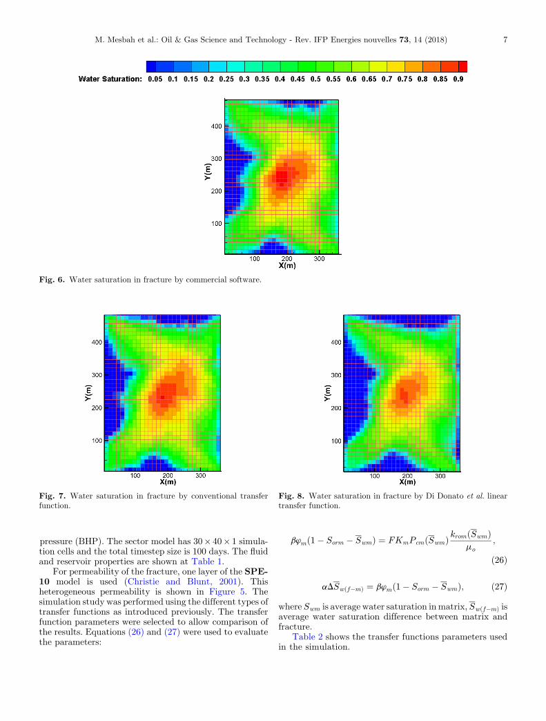
Fig. 6. Water saturation in fracture by commercial software.

Fig. 7. Water saturation in fracture by conventional transferfunction.

Fig. 8. Water saturation in fracture by Di Donato et al. lineartransfer function.

M. Mesbah et al.: Oil & Gas Science and Technology - Rev. IFP Energies nouvelles 73, 14 (2018) 7

pressure (BHP). The sector model has 30� 40� 1 simula-tion cells and the total timestep size is 100 days. The fluidand reservoir properties are shown at Table 1.

For permeability of the fracture, one layer of the SPE-10 model is used (Christie and Blunt, 2001). Thisheterogeneous permeability is shown in Figure 5. Thesimulation study was performed using the different types oftransfer functions as introduced previously. The transferfunction parameters were selected to allow comparison ofthe results. Equations (26) and (27) were used to evaluatethe parameters:

b’mð1� Sorm � SwmÞ ¼ FKmPcmðSwmÞ kromðSwmÞ;

mo

ð26Þ

aDSwðf�mÞ ¼ b’mð1� Sorm � SwmÞ; ð27Þ

where Swm is average water saturation inmatrix, Swðf�mÞ isaverage water saturation difference between matrix andfracture.

Table 2 shows the transfer functions parameters usedin the simulation.

Fig. 9. Water saturation in fracture by Kazemi et al. lineartransfer function.

Fig. 10. Water saturation in fracture by new linear transferfunction with constant coefficient.

Fig. 11. Water saturation in matrix by commercial software.

8 M. Mesbah et al.: Oil & Gas Science and Technology - Rev. IFP Energies nouvelles 73, 14 (2018)

5 Results and discussion

The results of the simulation studies and comparison ofdifferent transfer functions are summarized in this section.Toverify the results, IMEX-CMGa fully implicit simulationsoftware was applied. This simulation software uses theconventional transfer function (Computer-Modeling-Group, 2007). The water saturation and pressure distribu-tion in the fracture and matrix after 300 days of waterinjection are shown in the sector-model grids. The oil flowrate and cumulative volume of oil produced by theproduction wells using different transfer functions arerepresented. The TOF and streamlines are also shown.

Figures 6–10 representwater saturation inthe fracture.

Figures 11–15 represent water saturation in the matrix.Overall, Figures 6–15 show the results of different

transfer functions. It is clear that, in most cases, there arenegligible discrepancies. The figures show that watersaturation in the fracture is greater than in the matrix andcan be attributed to the greater permeability of thefracture. The fluid front has same pattern for both thematrix and fracture.

The figures showing water saturation in the matrixreveal that the difference in saturation was high. In fact,one reason for the extreme saturation difference is therange selected for matrix saturation range (0.21–0.34).

Figures 16–20 show the pressure distribution in thefracture.

Fig. 13. Water saturation in matrix by Di Donato et al. lineartransfer function.

Fig. 14. Water saturation in matrix by Kazemi et al. lineartransfer function.

Fig. 15. Water saturation in matrix by new linear transferfunction with constant coefficient.

Fig. 12. Water saturation in matrix by conventional transferfunction.

M. Mesbah et al.: Oil & Gas Science and Technology - Rev. IFP Energies nouvelles 73, 14 (2018) 9

It can be seen that the results of the commercialsoftware were slightly different from those of thestreamline method. With a decrease in the total timestepor size of the simulation grid cells, this difference becomesnegligible.

Figures 21–28 show the oil flow rate and cumulativevolume of oil produced by production wells from the start ofwater injection for a period of 500 days. The curves of thedifferent transfer function methods can be compared inthese figures.

The results do not differ significantly. The greatestdifference was for the results obtained from the Di Donatoet al. transfer function and was dependent on the value ofselected b.

The results of the proposed new transfer function aresimilar to that of the other solutions. The largest differencebetween the oil production rates obtained from theproposed transfer function and the commercial software

response is 15% for well A at the first timestep. Thisdifference gradually decreased in succeeding timesteps.

Figure 29 shows the TOF contour and Figure 30 showsthe streamlines after the first total timestep (100 days).

By investigation of the TOF grids (Fig. 29), the locationof the fluid front at different times can be predicted. Thestreamlines grids (Fig. 30) represent the flow pattern andcommunication between the injection well and productionwells. Asmentioned, the direction of the streamlines is fromthe injection well to the production wells. The compactionof streamlines at one part of the sector-model shows thehigher fluid velocity in that segment.

The TOF results shown in Figure 29 indicate that, afterthe injection of water, the breakthrough of water in well Coccurred in less than 100 days and, after a short time, waterbreakthrough occurred in well A. The water front thenreached wells B and D in 150 days. The streamlines inFigure 30 reveal that, the number of streamlines that end

Fig. 17. Pressure distributions in fracture by conventionaltransfer function.

Fig. 18. Pressure distributions in fracture by Di Donato et al.linear transfer function.

Fig. 19. Pressure distributions in fracture by Kazemi et al. lineartransfer function.

Fig. 20. Pressure distributions in fracture by new linear transferfunction with constant coefficient.

Fig. 16. Pressure distributions in fracture by commercial software.

10 M. Mesbah et al.: Oil & Gas Science and Technology - Rev. IFP Energies nouvelles 73, 14 (2018)

Fig. 22. Oil flow rate at production well B.

Fig. 21. Oil flow rate at production well A.Fig. 24. Oil flow rate at production well D.

Fig. 25. Cumulative volume of produced oil at production well A.

Fig. 23. Oil flow rate at production well C. Fig. 26. Cumulative volume of produced oil at productionwell B.

M. Mesbah et al.: Oil & Gas Science and Technology - Rev. IFP Energies nouvelles 73, 14 (2018) 11

Fig. 27. Cumulative volume of produced oil at productionwell C. Fig. 28. Cumulative volume of produced oil at productionwell D.

Fig. 29. Time-of-flight contour after the first total timestep(100 days).

Fig. 30. Streamlines after the first total timestep (100 days).

12 M. Mesbah et al.: Oil & Gas Science and Technology - Rev. IFP Energies nouvelles 73, 14 (2018)

in wells A and C are almost the same and are more than forwells B and D. This is consistent with the permeability ofthe fracture that is shown in Figure 5. Visualization of thestreamlines also indicates that the flow path from theinjection well to well A is more tortuous than the pathfrom the injection well to well C and this is the reason fordelayed breakthrough of the water front in well C.

The results of the commercial software and streamlinesimulator based on the conventional Kazemi et al. transferfunction should be the same because the applied transferfunction in both simulators is the same. The oil flow ratesreveal that the maximum differences between the commer-cial and streamline simulators for well A is 9% and that thisdifference decreases in the succeeding timesteps.

6 Conclusion

The current study simulated a heterogeneous fracturedreservoir using several transfer functions for the streamlinemethod. The results confirm the efficacy and capability ofthis simulation method. This method is equipped withstreamlines and TOF and uses them to gain the followingextra information over conventional simulation methods:

– the fluid flow pattern; – the relationship between wells; – analysis and interpretation of the flow path in thereservoir;

–

location of injected fluid front (e.g. tracer injection) atdifferent times.

M. Mesbah et al.: Oil & Gas Science and Technology - Rev. IFP Energies nouvelles 73, 14 (2018) 13

The streamline simulation method is a complementarymethod for conventional simulators of hydrocarbon reser-voirs. Comparison of the results of the presented transferfunctions, which are all based on the imbibition mechanism,showsthat theyare similar.Thedifferencesobservedrelate totheamountofwater saturation in the reservoir zones reachedby the water front. The rate of change in water saturation inthe linear transfer functions, especially for that of Di Donatoetal., is greater than for thatofKazemietal.Thisdiscrepancydoes not create a large difference in the amount of producedoil. As shown in Figures 21–24, the greatest differenceoccurred in the first timestep. In succeeding timesteps, theresults are closer and the graphs converge.

For single-layer heterogeneous fractured reservoirs,waterflooding was simulated using commercial softwareand an in-house streamline-based numerical code that usesthe DPSP reservoir model. The Kazemi et al. conventionaltransfer function was used in the commercial software. Inthe streamline simulator, in addition to the conventionaltransfer function, three linear transfer functions werereviewed and employed. The commercial software verifiedthe results of the streamline simulator, especially for theKazemi et al. conventional transfer function. By adjustingthe transfer function parameters, the results became moresimilar and all transfer functions were fairly acceptable.

The transfer functions discussed in this research are theKazemi et al. conventional transfer function, the Di Donatoetal. linear transfer function, theKazemietal. linear transferfunction and the proposed linear transfer function withconstantcoefficients.Theproposed lineartransfer function issimple to implement, has less calculation complexity, isappropriate for the streamline method and offers acceptableaccuracy when compared with other transfer functions.

List of symbols

K

permeability, m2

q

flow rate, m3

Sa

a phase saturation, dimensionless p pressure, kpa fa fractional flow of a phase T transfer function, 1/s Fs shape factor, 1/m2

U

Darcy velocity, m/s La fracture distance in a direction Pc capillary pressure, pa

Greek letters

ra

density of a phase, kg/m3

t

time-of-flight Dtsl local timestep Dtt total timestep ’ porosity l mobility ratio, 1/pa.s m viscosity, pa.s a, b transfer function constant coefficients, 1/s

References

Ahmadpour M., Siavashi M, Doranehgard M.H. (2016) Numeri-cal simulation of two-phase flow in fractured porous mediausing streamline simulation and IMPES methods and compar-ing results with a commercial software, J. Cent. South Univ. 23,10, 2630–2637.

Al-Huthali A., Datta-Gupta A. (2004) Streamline simulation ofcounter-current imbibition in naturally fractured reservoirs, J.Pet. Sci. Eng. 43, 3–4, 271–300.

Baker R. (2001) Streamline technology: reservoir historymatching and forecasting its success, limitations, and future,J. Can. Pet. Technol. 40, 4, 23–27.

Barenblatt G.I., Zheltov I.P., Kochina I.N. (1960) Basic conceptsin the theory of seepage of homogeneous liquids in fissured rocks[strata], J. Appl. Math. Mech. 24, 5, 1286–1303.

Batycky R.P, Blunt M.J., Thiele M.R. (1997) A 3D field-scalestreamline-based reservoir simulator, SPE Reserv. Eng. 12, 04,246–254.

Biagi J., Agarwal R., Zhang Z. (2016) Simulation andoptimization of enhanced gas recovery utilizing CO2, Energy94, 7, 78–86.

Bourbiaux B. (2010) Fractured reservoir simulation: a challeng-ing and rewarding issue, Oil Gas Sci. Technol. � Rev. IFP 65,2, 227–238.

Bourbiaux B., Cacas M.C., Sarda S., Sabathier J.C. (1998) Arapid and efficient methodology to convert fracturedreservoir images into a dual-porosity model, Rev. IFP53, 6, 785–799.

Brooks R., Corey T. (1964) HYDRAU uc properties of porousmedia, Hydrology Papers, Colorado State University 24.

Chen Z., Huan G., Ma Y. (2006) Computational methods formultiphase flows in porous media, SIAM, Philadelphia, USA.

Choobineh M.J., Siavashi M., Nakhaee A. (2015) Optimization ofoil production in water injection process using ABC and SQPalgorithms employing streamline simulation technique, Mod-ares Mech. Eng. 15, 5, 227–238.

Christie M.A., Blunt M.J. (2001) Tenth SPE comparativesolution project: a comparison of upscaling techniques, in:SPE Reservoir Simulation Symposium, Society of PetroleumEngineers.

Computer-Modeling-Group (2007) Launcher user’s guide, com-puter modeling group ltd, calgary, advanced oil/gas reservoirsimulator.

Datta-Gupta A., KingM.J. (2007). Streamline simulation: theoryand practice, Society of Petroleum Engineers Richardson,Richardson, TX, USA.

de Swaan A. (1978) Theory of waterflooding in fracturedreservoirs, Soc. Pet. Eng. J. 18, 02, 117–122.

Di Donato G., Blunt M.J. (2004) Streamline-based dual-porositysimulation of reactive transport and flow in fracturedreservoirs, Water Resour. Res. 40, 4, W04203.

Di Donato G., HuangW., BluntM. (2003). Streamline-based dualporosity simulation of fractured reservoirs, in: SPE AnnualTechnical Conference and Exhibition, Society of PetroleumEngineers.

Doranehgard M.H., Siavashi M. (2018) The effect of temperaturedependent relative permeability on heavy oil recovery duringhot water injection process using streamline-based simulation,Appl. Therm. Eng. 129, 11, 106–116.

14 M. Mesbah et al.: Oil & Gas Science and Technology - Rev. IFP Energies nouvelles 73, 14 (2018)

Gilman J.R. (2003) Practical aspects of simulation of fracturedreservoirs, in: International Forum on Reservoir Simulation,Buhl, Baden-Baden, Germany.

Gilman J.R., Kazemi H. (1983) Improvements in simulation ofnaturally fractured reservoirs, SPE J. 23, 4, 695–707.

Hassane T.F.R. (2013) The application of streamline reservoirsimulation calculations to the management of oilfield scale,Heriot-Watt University, Edinburgh, Scotland, UK.

Jerbi C., Fourno A., Noetinger B., Delay F. (2017) A newestimation of equivalent matrix block sizes in fractured mediawith two-phase flow applications in dual porosity models,J. Hydrol. 548, 40, 508–523.

Kazemi H., Merrill L.S. Jr., Porterfield K.L., Zeman P. (1976)Numerical simulation of water-oil flow in naturally fracturedreservoirs, Soc. Pet. Eng. J. 16, 06, 317–326.

Landereau P., Noetinger B., Quintard M. (2001) Quasi-steadytwo-equation models for diffusive transport in fractured porousmedia: large-scale properties for densely fractured systems,Adv. Water Resour. 24, 8, 863–876.

LeBlanc J.L., Caudle B.H. (1971) A streamline model forsecondary recovery, Soc. Pet. Eng. J. 11, 01, 7–12.

Lemonnier P., Bourbiaux B. (2010) Simulation of naturallyfractured reservoirs. State of the art, Part 1-Physical mecha-nisms and simulator formulation, Oil Gas Sci. Technol. � Rev.IFP 65, 2, 239–262.

Noetinger B., Roubinet D., Russian A., Le Borgne T., Delay F.,Dentz M., de Dreuzy J.-R., Gouze P. (2016) Random walkmethods for modeling hydrodynamic transport in porous andfractured media from pore to reservoir scale, Transp. PorousMedia 115, 2, 345–385.

Pollock D.W. (1988) Semianalytical computation of path lines forfinite-difference models, Groundwater 26, 6, 743–750.

Sarma P., Aziz K. (2004). New transfer functions for simulation ofnaturally fractured reservoirs with dual porosity models, in:SPE Annual Technical Conference and Exhibition, Society ofPetroleum Engineers.

Siavashi M., BluntM.J., RaiseeM., Pourafshary P. (2014) Three-dimensional streamline-based simulation of non-isothermaltwo-phase flow in heterogeneous porous media, Comput. Fluids103, 10, 116–131.

Siavashi M., Tehrani M.R., Nakhaee A. (2016) Efficient particleswarm optimization of well placement to enhance oil recoveryusing a novel streamline-based objective function, J. EnergyResour. Technol. 138, 5, 052903.

Thiele M.R. (2001) Streamline simulation, in: Proc. SixthInternational Forum on Reservoir Simulation, citeseer.

Vitoonkijvanich S., AlSofi A.M., Blunt M.J. (2015) Design offoam-assisted carbon dioxide storage in a North Sea aquiferusing streamline-based simulation, Int. J. Greenh. Gas Control33, 12, 113–121.