Streaming and storing CineGrid data: A study on optimization · PDF fileStreaming and storing...

System and Network Engineering

Research Project 2

Master of Science Program

Academic year 2007–2008

Streaming and storing CineGrid data:A study on optimization methods

by

Sevickson [email protected]

UvA Supervisor : Dr. Ir. Cees de Laat

Project Supervisors : Dr. Paola Grosso

MSc Ralph Koning

Research Project report for System and Network Engineering, University of Amsterdam, theNetherlands, for RP2 academic year 2007–2008.

This document is c© 2008Sevickson Kwidama [email protected].

Some rights reserved: this document is licensed under the Creative Commons Attribution 3.0Netherlands license. You are free to use and share this document under the condition that youproperly attribute the original authors. Please see the following address for the full license condi-tions: http://creativecommons.org/licenses/by/3.0/nl/deed.en

Cover image: A combination of a movie reel and the world, is meant to symbolize the co-operationaround the world through CineGrid. Source: http://www.stockxpert.com/.

Version 1.0.0 and compiled with LATEX on July 7, 2008.

Abstract

CineGrid enables participants to stream high-quality digital media, for collaboration anddemonstration purposes.

CineGrid has two possible streaming solutions, Scalable Adaptive Graphics Environment(SAGE) and NTT jpeg2000 codec.SAGE is specialized middleware software for enabling data, high-definition video and high-resolution graphics to be streamed in real-time, this depends heavily on the hardware used.

NTT jpeg2000 codec is the other streaming solution that is discussed in this paper.This setup uses hardware implementation to compress and decompress streams. The advan-tage that this setup has on SAGE is that the hardware does not influence the stream.The compression rate of NTT jpeg2000 codec greater is than the rate of SAGE, this wouldsuggest that less bandwidth is needed to stream high-quality digital media.

The local filesystem and NFS is used currently to store the CineGrid data, this form doesnot meet the requirements of the CineGrid network. The requirements are large and scalablestorage space and read speeds higher than the local filesystem and NFS.One of the possible solutions to meet the requirements is GlusterFS.GlusterFS can be implemented in a test setup, to look at the stability over long term. Theread speed of GlusterFS can become greater than the read speed of the local filesystem.

Contents

1 Introduction 5

2 CineGrid 6

3 Benchmarking 83.1 Streaming tests . . . . . . . . . . . . . . . . . . . . . . . . . . . . . . . . . . . . . . 83.2 Filesystem tests . . . . . . . . . . . . . . . . . . . . . . . . . . . . . . . . . . . . . . 9

4 SAGE vs NTT jpeg2000 codec 114.1 SAGE . . . . . . . . . . . . . . . . . . . . . . . . . . . . . . . . . . . . . . . . . . . 11

4.1.1 Test Method . . . . . . . . . . . . . . . . . . . . . . . . . . . . . . . . . . . 124.2 NTT jpeg2000 codec . . . . . . . . . . . . . . . . . . . . . . . . . . . . . . . . . . . 14

4.2.1 Test Method . . . . . . . . . . . . . . . . . . . . . . . . . . . . . . . . . . . 144.3 Results . . . . . . . . . . . . . . . . . . . . . . . . . . . . . . . . . . . . . . . . . . . 15

4.3.1 SAGE . . . . . . . . . . . . . . . . . . . . . . . . . . . . . . . . . . . . . . . 15

5 GlusterFS 205.1 Current situation . . . . . . . . . . . . . . . . . . . . . . . . . . . . . . . . . . . . . 205.2 GlusterFS . . . . . . . . . . . . . . . . . . . . . . . . . . . . . . . . . . . . . . . . . 205.3 Test Method . . . . . . . . . . . . . . . . . . . . . . . . . . . . . . . . . . . . . . . 215.4 Results . . . . . . . . . . . . . . . . . . . . . . . . . . . . . . . . . . . . . . . . . . . 225.5 Results w/ Performance Translators . . . . . . . . . . . . . . . . . . . . . . . . . . 24

6 Future Work 26

7 Conclusion 26

8 Acknowledgments 27

Bibliography 28

Appendices 29

A GlusterFS Installation 29

B GlusterFS Configuration 31B.1 Server Configuration file . . . . . . . . . . . . . . . . . . . . . . . . . . . . . . . . . 31B.2 Client Configuration file . . . . . . . . . . . . . . . . . . . . . . . . . . . . . . . . . 31B.3 Server Configuration file w/ Performance Translators . . . . . . . . . . . . . . . . . 32B.4 Client Configuration file w/ Performance Translators . . . . . . . . . . . . . . . . . 32

List of Tables

1 Digital Media Formats. Source: [7] . . . . . . . . . . . . . . . . . . . . . . . . . . . 72 Video differences . . . . . . . . . . . . . . . . . . . . . . . . . . . . . . . . . . . . . 133 Maximum read speed: Local, NFS, GlusterFS . . . . . . . . . . . . . . . . . . . . . 234 Maximum read speed: GlusterFS with Performance Translators . . . . . . . . . . . 25

List of Figures

1 GLIF World Map. Source: [6] . . . . . . . . . . . . . . . . . . . . . . . . . . . . . . 62 SAGE Architecture. Source: [2] . . . . . . . . . . . . . . . . . . . . . . . . . . . . . 113 Infrastructure used in SAGE tests. . . . . . . . . . . . . . . . . . . . . . . . . . . . 124 Infrastructure used in NTT tests. . . . . . . . . . . . . . . . . . . . . . . . . . . . . 155 Log SAGE Manager. T: TCP stream, B: UDP stream . . . . . . . . . . . . . . . . 166 CPU load UDP stream SAGE Manager/Renderer . . . . . . . . . . . . . . . . . . . 177 CPU load Display node. L: UDP stream, R: TCP stream . . . . . . . . . . . . . . 188 Stream fluctuation . . . . . . . . . . . . . . . . . . . . . . . . . . . . . . . . . . . . 199 GlusterFS storage design. Source: [21] . . . . . . . . . . . . . . . . . . . . . . . . . 2110 Infrastructure used in GlusterFS tests. . . . . . . . . . . . . . . . . . . . . . . . . . 22

4

1 INTRODUCTION

1 Introduction

CineGrid[1] Open Content Exchange (COCE) is a platform and architecture to stream CineGrid4K-content to different 4K-suitable locations. 4K stands for fourthousand× twothousand pixels,this is approximately 4× the HD quality nowadays.

Transport and streaming in CineGrid is done using either the Scalable Adaptive Graphics En-vironment (SAGE)[2] or the NTT hardware jpeg2000 codec[3]. These setups compress and de-compress the stream to make it possible to travel over 1 Gbps connections and still be able todeliver 4K-content on screen.These two setups have totally different approaches and a comparison has not yet been made be-tween them.The research question that summarizes this part of the research is:

How do SAGE and NTT jpeg2000 codec compare against each other, regarding networkstreams?

Another aspect of the research is the testing of GlusterFS[4] as a suitable storage system forCineGrid. The currently used system, NFS, does not meet the streaming requirements; whilethe research of a previous System and Network Engineering (SNE) student[5] pointed out thatGlusterFS would be a good alternative. I will build a test setup to test the performance ofGlusterFS to see if it truly can improve the current situation.The research question that summarizes this part of the research is:

Can GlusterFS improve the performance of the CineGrid storage?

In this document I will be looking at the different aspects given above.First I will give some background information about CineGrid in chapter 2 on the following page,and about benchmarking in chapter 3 on page 8 in conjunction with the different tools that I willuse.The two parts of my research project will be explained individually in chapter 4 on page 11 andchapter 5 on page 20.Closing this document I will give possible future work in chapter 6 on page 26 and some conclusionsin chapter 7.

5

2 CINEGRID

2 CineGrid

CineGrid is the basis for my research. In this chapter I will explain what CineGrid is and whatit’s purpose is.CineGrid, started in 2006 as a non-profit international organization. Nowadays CineGrid hasmembers from different countries. Some of the countries that are members in this organizationare: Japan, Netherlands, USA.The mission of CineGrid as stated on their website[1]:

CineGrid’s mission is to build an interdisciplinary community focused on the research,development, and demonstration of networked collaborative tools, enabling the pro-duction, use and exchange of very high-quality digital media over high-speed photonicnetworks.

The transport and streaming of high-quality digital media is made possible by a virtual interna-tional organization, the Global Lambda Integrated Facility (GLIF). This organization promotes theparadigm of lambda networking to support demanding scientific applications. Lambda networkingis the use of different ’colors’ or wavelengths of (laser) light in fibres for separate connections. Eachwavelength is called a ’lambda’[6].GLIF is one of the possible ways to transport and stream very high-quality digital media.

CineGrid uses the optical networks (lambda’s) of GLIF for intercontinental transport and stream-ing of the CineGrid content.In figure 1 I give the most recent map of the lambda connections around the world.

Figure 1: GLIF World Map. Source: [6]

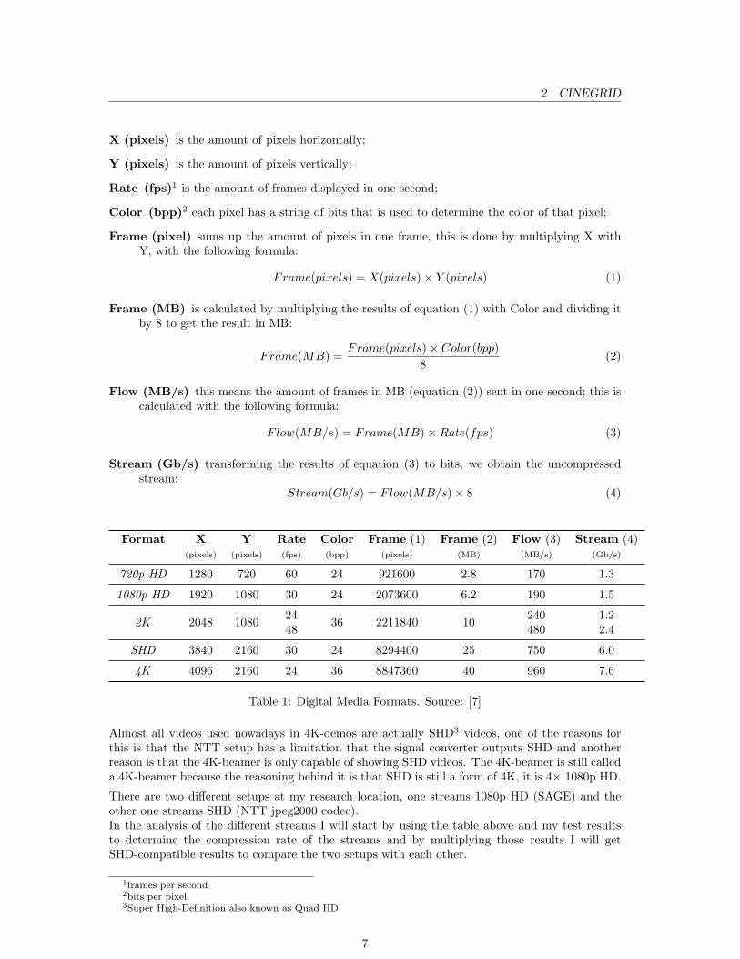
One of the high-quality digital media formats that is available in CineGrid is called 4K. This isroughly 4× 1080p HD quality which is viewable on HD televisions. In table 2 on the following pageI give a comparison between different formats. This comparison gives an idea of the differencebetween “smaller” media formats and 4K.

The characteristics of each format is displayed in a row in the format table.

6

2 CINEGRID

X (pixels) is the amount of pixels horizontally;

Y (pixels) is the amount of pixels vertically;

Rate (fps)1 is the amount of frames displayed in one second;

Color (bpp)2 each pixel has a string of bits that is used to determine the color of that pixel;

Frame (pixel) sums up the amount of pixels in one frame, this is done by multiplying X withY, with the following formula:

Frame(pixels) = X(pixels)× Y (pixels) (1)

Frame (MB) is calculated by multiplying the results of equation (1) with Color and dividing itby 8 to get the result in MB:

Frame(MB) =Frame(pixels)× Color(bpp)

8(2)

Flow (MB/s) this means the amount of frames in MB (equation (2)) sent in one second; this iscalculated with the following formula:

Flow(MB/s) = Frame(MB)×Rate(fps) (3)

Stream (Gb/s) transforming the results of equation (3) to bits, we obtain the uncompressedstream:

Stream(Gb/s) = Flow(MB/s)× 8 (4)

Format X Y Rate Color Frame (1) Frame (2) Flow (3) Stream (4)(pixels) (pixels) (fps) (bpp) (pixels) (MB) (MB/s) (Gb/s)

720p HD 1280 720 60 24 921600 2.8 170 1.3

1080p HD 1920 1080 30 24 2073600 6.2 190 1.5

2K 2048 1080 24 36 2211840 10 240 1.248 480 2.4

SHD 3840 2160 30 24 8294400 25 750 6.0

4K 4096 2160 24 36 8847360 40 960 7.6

Table 1: Digital Media Formats. Source: [7]

Almost all videos used nowadays in 4K-demos are actually SHD3 videos, one of the reasons forthis is that the NTT setup has a limitation that the signal converter outputs SHD and anotherreason is that the 4K-beamer is only capable of showing SHD videos. The 4K-beamer is still calleda 4K-beamer because the reasoning behind it is that SHD is still a form of 4K, it is 4× 1080p HD.

There are two different setups at my research location, one streams 1080p HD (SAGE) and theother one streams SHD (NTT jpeg2000 codec).In the analysis of the different streams I will start by using the table above and my test resultsto determine the compression rate of the streams and by multiplying those results I will getSHD-compatible results to compare the two setups with each other.

1frames per second2bits per pixel3Super High-Definition also known as Quad HD

7

3 BENCHMARKING

3 Benchmarking

Benchmarks are used to measure the time needed by a computer to execute a specified task. It isassumed that this time is related to the performance of the computer system and that the sameprocedure can be applied to other systems, so that comparisons can be made between differenthardware/software configurations.

From the definition of a benchmark, one can deduce that there are two basic procedures forbenchmarking:

• Measuring the time it takes for the system being examined to loop through a fixed numberof iterations of a specific piece of code.

• Measuring the number of iterations of a specific piece of code executed by the system underexamination in a fixed amount of time.[8]

In the benchmark tests that I will perform, the first procedure will be measured, meaning measurethe time it takes a computer system to run a specific procedure.

3.1 Streaming tests

In the tests that I will perform between the two different architectures the following tests will bedone:

• CPU load;

• Network performance and traffic behavior.

The CPU load will be monitored using the command “top”.This program gives real-time information about processes running on the system. The program isused with the following syntax:

top -b -d 0.5 > load.output# -b, batch-mode, useful for sending output to file# -d, delay between samples taken# > load.output, write the results to a file

I chose top because it is a standard tool available on Linux. By using a standard tool we increasethe possibility in reproducibility and standardization.The way that top calculates the load is by taken the CPU time of a process in a specific timeinterval, divide it against that time interval, multiply it by 100 to get the load percentage. Anoptional step is to divide that percentage against the amount of CPU cores in that system to getthe load per CPU.The CPU load percentage can be calculated with the following formula:

% CPULoad(t) =

∆T (t)t

× 100

# CPU ′s

To monitor and display the network performance, I chose Wireshark[9]. Wireshark is a proventool for packet capturing and analysis, it also has a graphing possibility to display traffic behavior.I will first capture the packets with tcpdump, tcpdump is a command-line program for capturingpackets, after that the captured packets are imported in Wireshark for analysis. To use tcpdumpin command-line the following command will be used:

8

3.2 Filesystem tests 3 BENCHMARKING

tcpdump -i eth -tt -v -w net.output host IP and tcp and not port ssh# -i eth, is the interface to listen to# -tt, print a timestamp# -v, level 1 verbose# -w net.output, file to write output to# host IP and tcp and not port ssh is the capture filterused to capture only not-ssh-TCP packets from and to that IP

SAGE keeps a log during streaming that can be used for my analysis. The output is a framenumber,the bandwidth used for streaming the video to the display and bandwidth available for compression.Furthermore it outputs the frames per second (fps) compressed and sent to the diplay.

By using this setup, later analysis can be done on the output. A graph of the tcpdump can bemade with the IO graph option in Wireshark, to display the traffic behavior. By using gnuplotgraphs can be made of the load and the SAGE log.

3.2 Filesystem tests

In the GlusterFS tests the read throughput will be measured, with the following tools:

• dd

• iozone

Dd is a tool to convert and copy a file, according to the man page[10]. This tool is also a standardtool available on Unix and Linux systems.The output of a copy operation can be used to measure the overall read throughput on block level.A block is a sequence of bytes or bits, with a nominal length (a block size). Most file systems arebased on a block device, which is a level of abstraction for the hardware responsible for storingand retrieving specified blocks of data[11].Different block sizes can have different throughput results.

Dd is used in the following manner:

dd if=inputfile of=outputfile/device# if=inputfile, specify the file that will be used to read from# of=outputfile/device, specify the file or device to sent the file toin this case /dev/null to measure only the read and not the write

# the output of this command will be a summary of the speed taken to copy file

Iozone[12] is a filesystem benchmark tool. This tool works on the file level.File level storage is exchanged between systems in client/server interactions. The client uses thefile’s name and is not interested how the file is saved. The server performs the block level storageoperations to read or write the data from a storage device[13].This tool is used to benchmark how the read throughput is with the filesystem overhead.The syntax and options used are:

iozone -e -i0 -i1 -r 16kb -s 7G -f iozone.tmp# -e, flush timings are included in the results# -i0, this is always needed, to make the file for the rest of the tests# -i1, measure the performance of reading a file# -r 16k, block size used# -s 7G, size of the file used in the tests# -f iozone.tmp, temporary file that was made with -i0 for the -i1 tests

9

3.2 Filesystem tests 3 BENCHMARKING

In the example of iozone above I use a filesize of 7GB, this is also the filesize that is used in thetests with dd. I use a 7GB file to make sure that no caching influences the test results and that Iget the throughput speed.A rule of thumb is use 2× the amount of RAM in the system to avoid caching[14].

I use the two tools above to measure different aspects of the read throughput:

• dd is a PIO transfer meaning the data is first sent through the processor, this measurementis done on block level;

• iozone is used to measure read throughput on file level.

The servers that I will use for my tests are part of the Rembrandt cluster [15].The Rembrandt cluster is a cluster owned by UvA, dedicated to support the OptIPuter node atAmsterdam Lighthouse, the research lab at SARA.[15]Nodes 1-7 in the Rembrandt cluster will be used in this project, the components that are relevantto my research project are:

• OS: Fedora Core 6

• Network: Gigabit Ethernet (GigE)

• Processor: Dual 64-bit CPUs (Opteron, 2.0 GHz)

• Memory: 4 GB (Rembrandt5 has less memory: 1 GB)

• Storage: Hardware-RAID (Serial ATA disk 250 GB×11, RAID 0)

10

4 SAGE VS NTT JPEG2000 CODEC

4 SAGE vs NTT jpeg2000 codec

4.1 SAGE

Scalable Adaptive Graphics Environment (SAGE)[2] is specialized middleware for enabling data,high-definition video and high-resolution graphics to be streamed in real-time, from remotelydistributed compression and storage clusters to tiled displays over ultra-high speed networks.[16]It can also be seen as a graphics streaming architecture. This architecture was primarily developedwith the thought of supporting collaborative scientific visualization environments and allow user-definable layouts on the displays.[17]I will use SAGE in this research project to stream videos to one high-definition display.

The architecture of SAGE, shown in figure 2, consists of the following components:

1. Free Space Manager (FSManager)

2. SAGE Application Interface Library (SAIL)

3. SAGE Receivers

4. UI clients

Figure 2: SAGE Architecture. Source: [2]

The FSManager is the window manager for SAGE. It can be compared with the Xserver on Linuxsystems. One of the most important differences with the Xserver is that this manager can scaleto many more displays. This component manages the displays by receiving window positions andother commands from the UI clients and sends control messages to SAIL nodes or the SAGEreceivers to update the displays.

SAIL is the layer between an application that is streaming and the displays. This componentcommunicates with the FSManager and streams directly to the SAGE receivers. By using thiscomponent it becomes easy to program and use “standard” applications in the streaming archi-tecture.

11

4.1 SAGE 4 SAGE VS NTT JPEG2000 CODEC

SAGE Receiver is a physical computer connected directly to one or more displays. This receiverreceives commands directly from the FSManager or indirectly by receiving the streams from SAIL.

UI Clients can be a Graphical User Interface (GUI), text-based console or tracked devices. A usercan use this to control the stream to the tiled displays by sending control messages (commands)to the FSManager and the UI client receives the status of the streams and displays.

SAGE can stream content with TCP or UDP.TCP is used for short distances because the latency is negligible in retransmission, after a lostpacket or NACK. UDP on the other hand is used in longer distances to stream content. Thelatency in longer distances is too great to retransmit without disturbing the displayed stream.

SAGE uses DXT to compress and decompress video, meaning it compresses and decompressesevery frame independently. The output of the codec process is a sequence of still images.DXT produces a compressed stream bandwidth of 250 Mb/s for a 1080p HD and 800 Mb/s for aSHD stream.[18]

SAGE functions in the following manner:

1. FSManager makes an ssh connection to the SAGE Receiver(s), to start the process thatreceives the stream, uncompresses it and streams to the display;

2. FSManager also sends the streaming commands to SAIL;

3. A streaming application compresses the stream and sends it with the help of SAIL to theReceiver.

4.1.1 Test Method

The infrastructure that I used in the tests is displayed in figure 3.In this setup Rembrandt4 is the FSManager. The application that streams the video with SAILis also available on Rembrandt4. The mac-mini is the SAGE receiver that sends the stream to thedisplay.

Figure 3: Infrastructure used in SAGE tests.

12

4.1 SAGE 4 SAGE VS NTT JPEG2000 CODEC

Doing the tests with SAGE, I made the following assumptions:

• tcpdump captures all packets in the limit of bandwidth;

• top is non-destructive, meaning it does not influence the SAGE setup.

The tools described in section 3.1 on page 8 will be used in the following manner in the SAGEtests:

top This tool will be executed on Rembrandt4 and the Mac-mini to register the percent of theCPU used by the SAGE utilities.

tcpdump This tool will also be executed on Rembrandt4 and Mac-mini to capture the SAGEpackets, this tool is used to measure the bandwidth usage, lost packets (retransmissions)and it will be used to graph the traffic signature, the tools are executed on both endpointsto see if there is change on the way to the endpoints.

SAGE log The log is kept on the manager, this logs the compression bandwidth, bandwidth tothe diplay, frames per second compressed and send to the display. This log is taken fromthe application layer, the results can be used to compare the bandwidth given by tcpdump.

The two tests that I have described above are the basic tests that I will use to get all the informationto later analyze and document. I had the idea to run the tests five times to make sure that nounknown variables would influence the stream. But after doing the UDP stream test five timesit was noted that doing the test five times was not necessary and two times would also sufficebecause the tests were done in a stable controlled environment.I first made a script to automate the tests but when I started the tests, it was noticed that theuse of the script takes too much processor time and therefore influences the stream by diminishingthe amount of frames compressed and sent per second.This would suggest that the compression process and streaming can be easily influenced.That is why the script was eventually not used, the commands were executed in separate tests.

Two different videos were used in the tests:

7Bridges This is a video made from a boat while travelling under several bridges in Amsterdam.

PragueTrain This one is a video of a steam locomotive passing by in Prague.

In table 4.1.1 I give the similarities and differences between these two videos.

Video Length Size Rate Media(secs) (GB) (fps) Format

7Bridges 138 4.3 30 1080p HD

PragueTrain 97 2.5 24 1080p HD

Table 2: Video differences

I used these videos to see if there would be difference in the output, but no difference was noted.That is why the PragueTrain video will be used for further analysis in section 4.3 on page 15. Ifind the Rate difference, when looking at the output, negligible.I chose this video because it is shorter, making it possible to gather more results in a shorteramount of time.

13

4.2 NTT jpeg2000 codec 4 SAGE VS NTT JPEG2000 CODEC

4.2 NTT jpeg2000 codec

NTT jpeg2000 codec has a different approach from SAGE, in the sense that it uses hardwareencoding and decoding instead of software-driven. This approach is taken because a hardwareimplementation is faster than a software implementation in the setup of NTT jpeg2000 codec.Jpeg2000 is the method used to compress and decompress the video stream. Jpeg2000 is anintra-frame codec just as DXT in SAGE.

The NTT setup has primarily two components: “jpeg2000 real-time codec” and “jpeg2000 server”.The jpeg2000 real-time codec is the component that compresses and decompresses the data at arate of 250 Megapixels per second, with a compressed data rate of up to 500 Mbps.[3] The jpeg2000real-time codec is a hardware node with the following components:

• OS: Linux

• Network: Gigabit Ethernet (GigE)

• Video Encoding/Decoding: 4× PCI-X JPEG 2000 codec boards with JPEG 2000 processingchips and 1 hardware real-time clock card to sync the cards[3]

This hardware node is directly connected to the displays; the maximum amount of displays thatone jpeg2000 real-time codec can handle is four.

As can be seen above this component only compresses and decompresses it doesn’t store the data,for that purpose one needs the jpeg2000 server.In iGrid 2005[19] they used a component called jpeg2000 server[3]. This hardware node does thestorage and sending the compressed video to the jpeg2000 real-time codec. The components are:

• OS: Linux

• Network: GigE

• Processor: Dual CPUs (Xeon, 3.0 GHz)

• Storage: Software-RAID (Serial ATA disk 250 GB×7, RAID 0, XFS file format)[3]

Looking at the specifications of jpeg2000 server above, it can be noted that it is not a storageserver specific for the jpeg2000 codec, this would mean that any storage server can be used.The jpeg2000 server is implemented in software, this is installed on node41[20]. This programreceives a data transfer command from the jpeg2000 real-time codec, reads the data from thestorage and writes the data periodically to the GigE network interface.[3]I will use this server for storage and the sending of the compressed video to the jpeg2000 real-timecodec.The transport method used in the NTT jpeg2000 codec is UDP.

4.2.1 Test Method

Due to unforeseen circumstances, I was not able to do the NTT jpeg2000 codec tests.

If it was possible to do the tests I would have used top and tcpdump in the same manner asexplained in 4.1.1 on page 12.

The infrastructure that I would have used in the tests is displayed in figure 4 on the next page.The NTT jpeg2000 codec is placed at SURFnet. That is why the SURFnet network would havebeen used to stream the video from node41, located at UvA, to the NTT jpeg2000 codec. Node41runs the jpeg2000 server process, called mserver, and the NTT jpeg2000 codec runs the mdecoderprocess, to decode and display the stream.

14

4.3 Results 4 SAGE VS NTT JPEG2000 CODEC

Figure 4: Infrastructure used in NTT tests.

4.3 Results

In this section I discuss the results from the SAGE setup. The tests were done several times butbelow I will only explain one test per subject, if there were noticeable differences between the testsI will point them out.The results will be explained by means of graphs.

4.3.1 SAGE

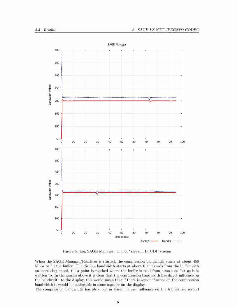
The logs discussed below were taken from the SAGE Manager/Renderer. This is the node thatcompresses and sends the stream to the node connected to the display. Figure 5 on the followingpage gives two graphs: TCP stream of the SAGE Manager/Renderer and the UDP stream. Thevariables that are displayed are:

Display This is the network bandwidth used from the Manager/Renderer to the display.

Render The SAGE Manager/Renderer’s internal bandwidth used to compress a video.

The Y-axis displays the amount of Mbps, the X-axis displays the seconds.

15


SAGE Manager

50

100

150

200

250

300

350

400

0 10 20 30 40 50 60 70 80 90 100

Ban

dwid

th (

Mbp

s)

50

100

150

200

250

300

350

400

0 10 20 30 40 50 60 70 80 90 100

Ban

dwid

th (

Mbp

s)

Time (secs)

Display Render

Figure 5: Log SAGE Manager. T: TCP stream, B: UDP stream

When the SAGE Manager/Renderer is started, the compression bandwidth starts at about 450Mbps to fill the buffer. The display bandwidth starts at about 0 and reads from the buffer withan increasing speed, till a point is reached where the buffer is read from almost as fast as it iswritten to. In the graphs above it is clear that the compression bandwidth has direct influence onthe bandwidth to the display, this would mean that if there is some influence on the compressionbandwidth it would be noticeable in some manner on the display.The compression bandwidth has also, but in lesser manner influence on the frames per second

16


compressed and sent.I believe that the gap between Render bandwidth and the Display bandwidth can be contributedto TCP or UDP packet processing. In the UDP graph the gap is less than in the TCP graphbecause UDP takes less processing.

The read operation from the buffer has 1 sec delay from the write operation, if this buffer sizeis increased it might increase the reliability of the stream by softening the effect on the displaybandwith of, forexample drops in the compression bandwidth.I would suggest to increase the buffer size and the delay so that the bandwidth to the display isnot influenced. This could be applied in both TCP and UDP cases.

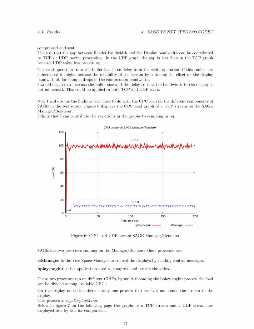
Now I will discuss the findings that have to do with the CPU load on the different components ofSAGE in the test setup. Figure 6 displays the CPU load graph of a UDP stream on the SAGEManager/Renderer.I think that I can contribute the variations in the graphs to sampling in top.

0

20

40

60

80

100

120

0 50 100 150 200

Load

(%

)

Time (0.5 sec)

CPU usage on SAGE Manager/Renderer

CPU1

CPU0

bplay-noglut fsManager

Figure 6: CPU load UDP stream SAGE Manager/Renderer

SAGE has two processes running on the Manager/Renderer these processes are:

fsManager is the Free Space Manager to control the displays by sending control messages.

bplay-noglut is the application used to compress and stream the videos.

These two processes run on different CPU’s, by multi-threading the bplay-noglut process the loadcan be divided among available CPU’s

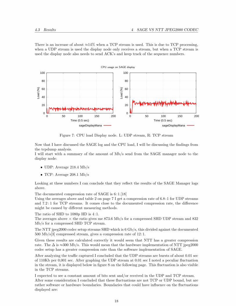
On the display node side there is only one process that receives and sends the stream to thedisplay.This process is sageDisplayMana.Below in figure 7 on the following page the graphs of a TCP stream and a UDP stream aredisplayed side by side for comparison.

17


There is an increase of about ≈14% when a TCP stream is used. This is due to TCP processing,when a UDP stream is used the display node only receives a stream, but when a TCP stream isused the display node also needs to send ACK’s and keep track of the sequence numbers.

CPU usage on SAGE display

0

20

40

60

80

100

0 50 100 150 200

Load

(%

)

Time (0.5 sec)

sageDisplayMana

0

20

40

60

80

100

0 50 100 150 200

Load

(%

)Time (0.5 sec)

sageDisplayMana

Figure 7: CPU load Display node. L: UDP stream, R: TCP stream

Now that I have discussed the SAGE log and the CPU load, I will be discussing the findings fromthe tcpdump analysis.I will start with a summary of the amount of Mb/s send from the SAGE manager node to thedisplay node:

• UDP: Average 218.4 Mb/s

• TCP: Average 208.1 Mb/s

Looking at these numbers I can conclude that they reflect the results of the SAGE Manager logsabove.

The documented compression rate of SAGE is 6:1.[18]Using the averages above and table 2 on page 7 I get a compression rate of 6.8:1 for UDP streamsand 7.2 : 1 for TCP streams. It comes close to the documented compression rate, the differencemight be caused by different measuring methods.

The ratio of SHD to 1080p HD is 4:1.The averages above × the ratio gives me 873.6 Mb/s for a compressed SHD UDP stream and 832Mb/s for a compressed SHD TCP stream.

The NTT jpeg2000 codec setup streams SHD which is 6 Gb/s, this divided against the documented500 Mb/s[3] compressed stream, gives a compression rate of 12:1.

Given these results are calculated correctly it would seem that NTT has a greater compressionrate. The ∆ is ≈300 Mb/s. This would mean that the hardware implementation of NTT jpeg2000codec setup has a greater compression rate than the software implementation of SAGE.

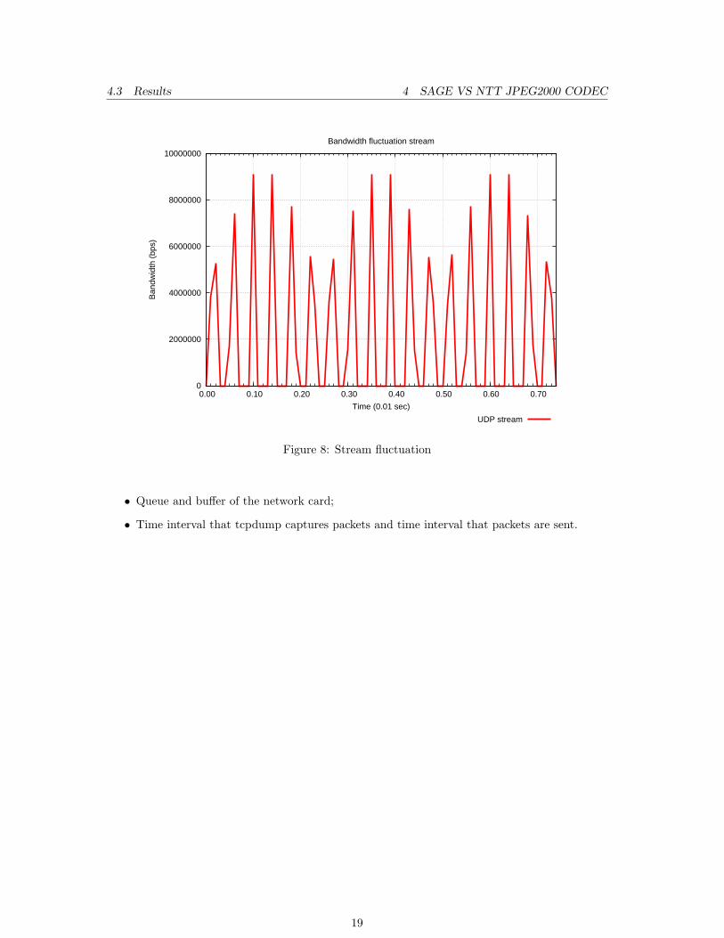
After analyzing the traffic captured I concluded that the UDP streams are bursts of about 0.01 secof 110Kb per 0,001 sec. After graphing the UDP stream at 0.01 sec I noted a peculiar fluctuationin the stream, it is displayed below in figure 8 on the following page. This fluctuation is also visiblein the TCP streams.

I expected to see a constant amount of bits sent and/or received in the UDP and TCP stream.After some consideration I concluded that these fluctuations are not TCP or UDP bound, but arerather software or hardware boundaries. Boundaries that could have influence on the fluctuationsdisplayed are:

18


0

2000000

4000000

6000000

8000000

10000000

0.00 0.10 0.20 0.30 0.40 0.50 0.60 0.70

Ban

dwid

th (

bps)

Time (0.01 sec)

Bandwidth fluctuation stream

UDP stream

Figure 8: Stream fluctuation

• Queue and buffer of the network card;

• Time interval that tcpdump captures packets and time interval that packets are sent.

19

5 GLUSTERFS

5 GlusterFS

This is the second part of my research project. Below I will give an overview of the currentsituation with NFS.GlusterFS architecture and installation will be discussed afterwards and the test methods andresults will be discussed.

5.1 Current situation

The setup that is currently used to store videos is to store them locally or by storing them onservers with NFS. NFS stores the videos independently on different servers, they are accessed withthe NFS protocol.These approaches have both their disadvantages when it comes to CineGrid. Local file disadvan-tages are, that the storage capacity does not increase fast enough to hold the terabytes of datasent and received from CineGrid. The storage bus speed is less than the network speed.NFS removes the short coming of bus speed of local storage but has other disadvantages, oneof the disadvantages is that the servers are accessed individually and the storage capacities areindividually sorted meaning that they can not be summed up to increase the storage capacity.

5.2 GlusterFS

GlusterFS uses the idea of using clusters of independent storage units and combine them into onelarge storage server. This concept can have performance increase compared to other networkedfilesystems, because every node has its own CPUs, memory, I/O bus, RAID storage and intercon-nect interface. These units can have an aggregated performance increase. GlusterFS is designedfor linear scalability for very large sized storage clusters.[21]

GlusterFS consists of different components:

GlusterFS Server and Client The server has the storage capability and exports the predefinedstorage amount so that the client can mount it.

GlusterFS Translators Translators are used to extend the filesystem capabilities through a welldefined interface.

GlusterFS Transport Modules Transport Modules are implemented by the Translators andthis module defines the method of transport. The methods defined at this moment inGlusterFS are TCP/IP, Infiniband userspace verbs (IB-verbs) and Infiniband socket directprotocol (IB-SDP).

GlusterFS Scheduler Modules The Scheduler Module does the load balancing between thedifferent storage servers.

GlusterFS Volume Specification Volume Specifications are configuration files to connect theservers to the clients.

The design of GlusterFS is displayed in figure 9 on the next page. The storage bricks in thefigure are actually the individual storage nodes. The storage clients are the clients that mount thestorage system to make use of it.On the bricks and the clients GlusterFS must be installed; there is one installation package forboth server and client. By using different commands you can choose for both server and clientexecutables or only one of them.

20

5.3 Test Method 5 GLUSTERFS

Figure 9: GlusterFS storage design. Source: [21]

5.3 Test Method

For testing the performance of a local file, NFS and GlusterFS, I first performed a dd and iozone ofthe local file system to have a base measurement. This base measurements was taken to calculatethe performance improvements achieved with GlusterFS.After taking the base measurements of the local filesystem I will also take the measurement ofNFS to have an idea of the performance of the current setup. I will use Rembrandt1 as NFS clientand Rembrandt2 as the NFS server.In the tests I use different block sizes to see if there are differences in throughput.

GlusterFS has many “Translators” that can be used to configure the filesystem to fulfill specificstorage needs. My research of GlusterFS will focus on performance improvements. The differenttranslators that can improve performance are:

1. Performance Translators

(a) Read Ahead Translator, improve reading by prefetching a sequence of blocks

(b) Write Behind Translator, to improve the write performance

(c) Threaded I/O Translator, is best used to improve the performance of concurrent I/O

(d) IO-Cache Translator, improves the speed of rereading a file

(e) Booster Translator, removes FUSE (Filesystem in USErspace) overhead

2. Clustering Translators

(a) Automatic File Replication Translator (AFR), mirroring capability

(b) Stripe Translator, striping capability

(c) Unify Translator, this sums up all the storage bricks and present them as one brick [4]

The stripe translator works a bit like RAID 0, in the sense that it divides the input file in blocksand saves that block on individual servers (disks in the case of RAID 0). This is done in theround-robin fashion. In theory this method is the best method to increase read performance, thatis why I will use this method in my tests.The other performance translators can later be added for more performance increase. I will onlyuse the stripe translator, this will give an idea of the minimum performance increase that can be

21

5.4 Results 5 GLUSTERFS

achieved when using GlusterFS.The installation of GlusterFS is discussed in Appendix A on page 29.

Figure 10: Infrastructure used in GlusterFS tests.

In figure 10 a schematic picture is given of the setup used in the storage tests.In the setup displayed above I will use Rembrandt1 as the GlusterFS client and respectivelyRembrandt2 for 1 server brick test, Rembrandt 2 and 6 for the two server test and Rembrandt 2,6 and 7 for the three server test.The setup used in the three server setup is displayed in Appendix B.1 and Appendix B.2.

5.4 Results

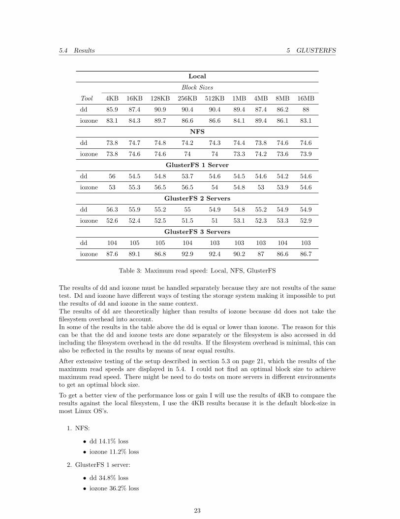
In this section I will be discussing my findings in the storage performance tests. Table 5.4 displaysthe results of the tests; the results are in MB/s.The results displayed in the table are the results of doing each test twice and taking the bandwidthresults with the maximum MB/s.

22

5.4 Results 5 GLUSTERFS

Local

Block Sizes

Tool 4KB 16KB 128KB 256KB 512KB 1MB 4MB 8MB 16MB

dd 85.9 87.4 90.9 90.4 90.4 89.4 87.4 86.2 88

iozone 83.1 84.3 89.7 86.6 86.6 84.1 89.4 86.1 83.1

NFS

dd 73.8 74.7 74.8 74.2 74.3 74.4 73.8 74.6 74.6

iozone 73.8 74.6 74.6 74 74 73.3 74.2 73.6 73.9

GlusterFS 1 Server

dd 56 54.5 54.8 53.7 54.6 54.5 54.6 54.2 54.6

iozone 53 55.3 56.5 56.5 54 54.8 53 53.9 54.6

GlusterFS 2 Servers

dd 56.3 55.9 55.2 55 54.9 54.8 55.2 54.9 54.9

iozone 52.6 52.4 52.5 51.5 51 53.1 52.3 53.3 52.9

GlusterFS 3 Servers

dd 104 105 105 104 103 103 103 104 103

iozone 87.6 89.1 86.8 92.9 92.4 90.2 87 86.6 86.7

Table 3: Maximum read speed: Local, NFS, GlusterFS

The results of dd and iozone must be handled separately because they are not results of the sametest. Dd and iozone have different ways of testing the storage system making it impossible to putthe results of dd and iozone in the same context.The results of dd are theoretically higher than results of iozone because dd does not take thefilesystem overhead into account.In some of the results in the table above the dd is equal or lower than iozone. The reason for thiscan be that the dd and iozone tests are done separately or the filesystem is also accessed in ddincluding the filesystem overhead in the dd results. If the filesystem overhead is minimal, this canalso be reflected in the results by means of near equal results.

After extensive testing of the setup described in section 5.3 on page 21, which the results of themaximum read speeds are displayed in 5.4. I could not find an optimal block size to achievemaximum read speed. There might be need to do tests on more servers in different environmentsto get an optimal block size.

To get a better view of the performance loss or gain I will use the results of 4KB to compare theresults against the local filesystem, I use the 4KB results because it is the default block-size inmost Linux OS’s.

1. NFS:

• dd 14.1% loss

• iozone 11.2% loss

2. GlusterFS 1 server:

• dd 34.8% loss


23

5.5 Results w/ Performance Translators 5 GLUSTERFS

3. GlusterFS 2 servers:

• dd 34.5% loss



• dd 21% gain

• iozone 5.4% gain

Following the results above I can say with certainty that GlusterFS can surpass the read speed ofthe local filesystem, thus three or more server bricks are used.It is interesting to note that there is minimal difference between the one server and the two serversetup. I think the reason for this is that changing from one server to two servers with stripingincreases the network and filesystem overhead making it seem like there is no improvement in theresults.For real improvements a minimum of three server bricks must be used, if less servers are availableit is better to keep using the local filesystem or NFS when talking about read performance.

After I concluded this, a chance was opened up to do GlusterFS tests on four and five servers. Ithought it would increase when more servers were used. But I did not see increase in the readspeed which I found strange. I thought maybe the maximum that one thread on the client canreceive was reached, that is why I increased the amount of GlusterFS threads on the client, thenon the server.But no improvement was noted.After discussing this problem with other members of SNE it was concluded that the 1 Gb connec-tion between the GlusterFS client and the servers was full. Taking the bandwidth results of thethree GlusterFS server setup, multiplying it with 8 to get the amount of Mb, and adding TCPoverhead we immediately see that the total bandwidth is close to the 1 Gb maximum.

The servers that I used as bricks were all homogeneous, when I used a system with less memorya decline was noted in the read performance.This would point out that GlusterFS is best used in a homogeneous architecture to get maximumperformance.

On a side note I don’t think GlusterFS is yet ready to be used in a distributed manner over anetwork connected to the Internet, the reason for this is that the version now available, version1.3, does not include encryption. However they are planning in incorporating this feature in futurereleases [4].Encryption is not a prerequisite in the architecture of CineGrid, as long as dedicated paths areused.

The observation that I have just given do not have consequences on the the CineGrid network andon my conclusions, but I thought it might be useful to keep this in mind when architecturing aGlusterFS network.

5.5 Results w/ Performance Translators

After it became clear that the 1 Gb connection between the GlusterFS client and GlusterFS serverswas the bottleneck, the connection was upgraded to a 10Gb connection.With this upgrade I decided to include some Performance Translators to give an idea of theperformance increases that can be achieved with GlusterFS when using Performance Translators.The Performance Translators that I used were:

• Read Ahead Translator

• Threaded I/O Translator

24

5.5 Results w/ Performance Translators 5 GLUSTERFS

I also included Rembrandt3 and Rembrandt4 to get results of four and five GlusterFS servers.In Appendix B.3 and Appendix B.4 I give the configurations that I used.The results in table 5.5 are given in the same manner as the results in table 5.4 on page 23.

GlusterFS 1 Server

Block Sizes

Tool 4KB 16KB 128KB 256KB 512KB 1MB 4MB 8MB 16MB

dd 89.9 95.6 83.4 91.4 93.3 88.4 83.4 79.7 91.7

GlusterFS 2 Servers

dd 103 119 122 122 123 123 121 118 118

GlusterFS 3 Servers

dd 294 323 323 304 265 262 259 269 261

GlusterFS 4 Servers

dd 306 336 326 303 263 305 260 263 278

GlusterFS 5 Servers

dd 315 331 333 308 270 260 260 265 260

Table 4: Maximum read speed: GlusterFS with Performance Translators

As you can see above, there is a big difference between GlusterFS results without PerformanceTranslators and GlusterFS results with Performance Translators. This would suggest that it is agood idea to use different Translators for different storage needs.Below I also give the performance gains in percentages compared to the Local Filesystem readspeed.

1. GlusterFS 1 server:

• dd 0.8% gain


• dd 19.9% gain


• dd 242.3% gain


• dd 256.2% gain


• dd 266.7% gain

25

7 CONCLUSION

6 Future Work

Now that you reached the end of my report on SAGE, NTT jpeg2000 codec and GlusterFS, Iwould like to make some suggestions for future work.

The NTT jpeg2000 codec test must be done, in the same manner I used in this document, to makea comparison between SAGE and NTT jpeg2000 codec.I would also suggest to build a SAGE setup that streams SHD to make a realistic comparisonbetween the SAGE setup and the NTT jpeg2000 codec setup.

The use of tools like strace can give a better understanding of the compression and streamingprocess of SAGE, and make it possible to make improvements to the SAGE setup.

A research project can investigate packet drops and increase the reliability of the streaming pro-cess. I did not discuss packet drops in this document, but it was brought to my attention duringthe research project that packet drops directly influence the stream displayed.At the moment no clear explanation is available for the packet drops.

Regarding GlusterFS, I think it can be implemented in a test network to look at it’s stability overlong term.If the stability is satisfactory, it should be implemented in the production network of CineGrid.By using GlusterFS in CineGrid it can increase the read performance of the Rembrandt clusterwhen streaming over long distances.There should also be some research on the different Translators to see which combination has themost performance increase.

7 Conclusion

I will mention the conclusions in the same order as this document.

SAGE is a implementation in the spirit of open source. It can be used on different Linux systems,but because it is implemented in software, it heavily depends on the hardware it runs on.I assume the calculations made with the SAGE results to get SHD stream are correct.The compression rate of NTT jpeg2000 codec is greater than the rate of SAGE. The differencebetween the setups is about ≈ 300 Mb/s.

The tests with NTT jpeg2000 codec were not possible, which means that I could not make anoverall comparison.NTT jpeg2000 codec is implemented in the hardware. This has the advantage over SAGE thatthe hardware does not influence the stream.Although NTT jpeg2000 codec is used in many different CineGrid installations, there is near tono documentation in English on the Internet, most of the documentation is in Japanese. On theother hand SAGE has been documented in many academic papers available via their website[2].

I conclude that GlusterFS can be implemented in a test setup, to look at the stability over longterm. The read speed of GlusterFS is greater than the local filesystem when three or more serverbricks are used.Good attention must be taken on the amount of bandwidth available when using GlusterFS,because it can easily become a bottleneck.

26

8 ACKNOWLEDGMENTS

8 Acknowledgments

Dear reader,

First I would like to give my praise to God for giving me life and this opportunity.

I would like to extend my gratitude to my two supervisors Dr. P. Grosso and MSc R. Koning fortheir time and guidance.I would also like to thank J. Roodhart for his help with GlusterFS.

SURFnet receives my thanks for their time spend in setting up the NTT jpeg2000 codec. Becauseof time restraints and unforeseen network problems I could not complete the tests with the NTTjpeg2000 codec setup.

I thank Dr. K. Koymans, J. van Ginkel and E. Schatborn for giving me the opportunity to doSystem and Network Engineering.Dr. Ir. C. de Laat for the choice of this Research Project and his advice.

Last but not least I would like to thank my parents for their time spend reviewing this paper andmy girlfriend for her patience.

With kind regards,

Sevickson Kwidama

27

REFERENCES REFERENCES

References

[1] Cinegrid. Cinegrid. Website. http://cinegrid.org/index.php.

[2] Electronic Visualization Laboratory. Sage. Website. http://www.evl.uic.edu/cavern/sage/index.php.

[3] Takashi Shimizu et. al. International real-time streaming of 4k digital cinema. Future Gen-eration Computer Systems, 22, May 2006.

[4] GlusterFS. Glusterfs. Website. http://www.gluster.org/.

[5] Daniel Sanchez. Design of store-and-forward servers for digital media distribution. Master’sthesis, University of Amsterdam, 2007.

[6] GLIF. Glif: the global lambda integrated facility. Website. http://www.glif.is/.

[7] Ralph Koning. Cinegrid on layer2 paths. Presentation at Terena Networking Conference,2008. http://tnc2008.terena.org/.

[8] Andre D. Balsa. Linux benchmarking - concepts. Website. http://linuxgazette.net/issue22/bench.html.

[9] Gerald Combs et al. Wireshark: Go deep. Website. http://www.wireshark.org/.

[10] die.net. dd(1) - linux man page. Website. http://linux.die.net/man/1/dd.

[11] Wikipedia. Wikipedia, the free encyclopedia. Website. http://en.wikipedia.org/.

[12] IOzone. Iozone filesystem benchmark. Website. http://www.iozone.org/.

[13] Mark Farley. Block and file level storage. Website. http://searchstorage.techtarget.com/expert/KnowledgebaseAnswer/0,289625,sid5_gci548225,00.html.

[14] Tim Verhoeven. Centos: How to test and monitor disk performance. Website. http://misterd77.blogspot.com/2007/11/how-to-test-and-monitor-disk.html.

[15] Advanced Internet Research. Rembrandt cluster. Website. http://www.science.uva.nl/research/air/network/rembrandt/index_en.html.

[16] Byungil Jeong et al. High-performance dynamic graphics streaming for scalable adaptivegraphics environment. 2006.

[17] Javid M. Alimohideen Meerasa. Design and implementation of sage display controller. 2003.

[18] Jason Leigh Luc Renambot, Byungil Jeong. Realtime compression for high-resolution content.2007.

[19] iGrid2005, 2005.

[20] Universiteit van Amsterdam. Cinegrid distribution center amsterdam. Website. http://cinegrid.uva.netherlight.nl/.

[21] GlusterFS. Glusterfs user guide v1.3. Website. http://www.gluster.org/docs/index.php/GlusterFS_User_Guide_v1.3.

28

A GLUSTERFS INSTALLATION

Appendices

A GlusterFS Installation

I first installed GlusterFS on my own test environment in OS34, before installing it on the Rem-brandt’s at UvA. I did this to first understand how the GlusterFS installation works and how itcan be configured. This was done in a test environment to minimize the impact that GlusterFSwould have it there was some problem.

GlusterFS was first installed in the Ubuntu 8.04 DomU under Xen at OS3 but this installationwas not successful, below I will discuss installation process and problems that I ran in while tryingto get GlusterFS to work.

To install GlusterFS in Ubuntu I first took care of the dependencies by issuing the followingcommand:

sudo apt-get install libtool gcc flex bison byacc

Also the kernel source (linux-source) are necessary if you want to compile the patched FUSEmodule for GlusterFS to use with the clients.This FUSE module has improvements to increase the I/O throughput of GlusterFS.

The installation of GlusterFS can be done in two methods, compile from source or install fromDebian package for Debian kernels or RPM and yum for ... kernels.I used the compilation from source method to understand the installation process for GlusterFS.To install the server for GlusterFS and the client without the FUSE improvements the followingcommands were used:

wget http://europe.gluster.org/glusterfs/1.3/glusterfs-CURRENT.tar.gztar -xzf glusterfs-CURRENT.tar.gzcd glusterfs-1.3.9./configure --prefix= #without the --prefix I got problems with the libraries

################### This is the output of ./configure ########################GlusterFS configure summary ##=========================== ### This line below informs that the client cannot be installed because FUSE ### is not correctly configured ##Fuse client : no ### The line below is yes when Infiniband verbs is installed for transport, ### default the transport method is TCP/IP ##Infiniband verbs : no ### This one is for the polling method for the server ##epoll IO multiplex : yes ##############################################################################

sudo make install

Like it is displayed above the installation does not install the client, this might be because FUSEis not installed or not correctly for configured to be used by GlusterFS.

Installation of FUSE was done with the following commands:4SNE Master study. https://www.os3.nl/

29

A GLUSTERFS INSTALLATION

wget http://europe.gluster.org/glusterfs/fuse/fuse-2.7.3glfs10.tar.gztar -xzf fuse-2.7.3glfs10.tar.gzcd fuse-2.7.3glfs10./configure --prefix=/usr --enable-kernel-modulemake installldconfigdepmod -armmod fuse # I receive an error when I try to remove the module, it says that it is in usemodprobe fuse

When I tried to install it on my Ubuntu 8.04 with kernel 2.6.24-19, I received the following error:

Making install in kernelmake[1]: Entering directory ‘/home/$user/fuse-2.7.3glfs10/kernel’make -C /usr/src/linux-headers-2.6.24-19-generic SUBDIRS=‘pwd‘ modulesmake[2]: Entering directory ‘/usr/src/linux-headers-2.6.24-19-generic’CC [M] /home/$user/fuse-2.7.3glfs10/kernel/dev.oCC [M] /home/$user/fuse-2.7.3glfs10/kernel/dir.o

/home/$user/fuse-2.7.3glfs10/kernel/dir.c: In function iattr_to_fattr:/home/$user/fuse-2.7.3glfs10/kernel/dir.c:1027: error: struct iattr has no member named ia_filemake[3]: *** [/home/$user/fuse-2.7.3glfs10/kernel/dir.o] Error 1make[2]: *** [_module_/home/$user/fuse-2.7.3glfs10/kernel] Error 2make[2]: Leaving directory ‘/usr/src/linux-headers-2.6.24-19-generic’make[1]: *** [all-spec] Error 2make[1]: Leaving directory ‘/home/$user/fuse-2.7.3glfs10/kernel’make: *** [install-recursive] Error 1

The conclusion that I made from this error is that Ubuntu made some changes in the function’iattr to fattr’ making it not possible to install the patched FUSE for the client in this versionof Ubuntu.That is why I downgraded my Ubuntu virtual machines to version 7.10 and I didn’t receive thiserror anymore.

After successfully installing the GlusterFS server and client on Ubuntu 7.10 I tried these steps onthe Rembrandt’s. The Rembrandt’s have Fedora Core 6 installed. When I tried to install it in myown home environment I got the following error:

test -z "/sbin" || mkdir -p -- "/sbin"/usr/bin/install -c ’mount.glusterfs’ ’/sbin/mount.glusterfs’/usr/bin/install: cannot create regular file ‘/sbin/mount.glusterfs’: Permission deniedmake[5]: *** [install-slashsbinSCRIPTS] Error 1make[5]: Leaving directory ‘/home/$user/glusterfs-1.3.9/xlators/mount/fuse/utils’make[4]: *** [install-am] Error 2make[4]: Leaving directory ‘/home/$user/glusterfs-1.3.9/xlators/mount/fuse/utils’make[3]: *** [install-recursive] Error 1make[3]: Leaving directory ‘/home/$user/glusterfs-1.3.9/xlators/mount/fuse’make[2]: *** [install-recursive] Error 1make[2]: Leaving directory ‘/home/$user/glusterfs-1.3.9/xlators/mount’make[1]: *** [install-recursive] Error 1make[1]: Leaving directory ‘/home/$user/glusterfs-1.3.9/xlators’make: *** [install-recursive] Error 1

First look at this error gives the idea that I’m trying to write in a directory that I don’t havepermission to write in, this is obvious because I only have write permissions in my own homedirectory.

30

B GLUSTERFS CONFIGURATION

But I receive this error also when I use my own home directory as environment for the /sbin.After discussing it with Jeroen Roodhart it was concluded that there was a bug in the Makefile.The bug is that the ./configure does not change all the path variables to the variables that I writeas –prefix.

After this the GlusterFS worked on the Rembrandt’s with no problem.

B GlusterFS Configuration

B.1 Server Configuration file

volume bricktype storage/posixoption directory /glusterfs/skwidama-exp

end-volume

volume servertype protocol/serveroption transport-type tcp/serversubvolumes brickoption auth.ip.brick.allow 192.168.192.*

end-volume

B.2 Client Configuration file

volume remote1type protocol/clientoption transport-type tcp/clientoption remote-host 192.168.192.12option remote-subvolume brick

end-volume


end-volume


end-volume

volume stripe0type cluster/stripeoption block-size *:1MBsubvolumes remote1 remote2 remote3

end-volume

31

B.3 Server Configuration file w/ Performance TranslatorsB GLUSTERFS CONFIGURATION

B.3 Server Configuration file w/ Performance Translators

volume bricktype storage/posixoption directory /glusterfs/skwidama-exp

end-volume

volume iottype performance/io-threadsoption thread-count 2option cache-size 32MBsubvolumes brick

end-volume

volume servertype protocol/serveroption transport-type tcp/serversubvolumes iotoption auth.ip.iot.allow 192.168.192.*

end-volume

B.4 Client Configuration file w/ Performance Translators

volume remote1type protocol/clientoption transport-type tcp/clientoption remote-host 192.168.192.12option remote-subvolume iot

end-volume


end-volume


end-volume


end-volume

volume remote5type protocol/client

32

B.4 Client Configuration file w/ Performance TranslatorsB GLUSTERFS CONFIGURATION

option transport-type tcp/clientoption remote-host 192.168.192.17option remote-subvolume iot

end-volume

volume stripe0type cluster/stripeoption block-size *:1MBsubvolumes remote1 remote2 remote3 remote4 remote5

end-volume

volume readaheadtype performance/read-aheadoption page-size 1MBoption page-count 20option force-atime-update offsubvolumes stripe0

end-volume

33

Streaming and storing CineGrid data: A study on optimization · PDF fileStreaming and storing...

Documents

Transcript of Streaming and storing CineGrid data: A study on optimization · PDF fileStreaming and storing...