
STREAM FISH RESPONSE TO INTERMITTENCY AND DRYING IN …
196
STREAM FISH RESPONSE TO INTERMITTENCY AND DRYING IN THE ICHAWAYNOCHAWAY CREEK BASIN by JESSICA L. DAVIS (Under the Direction of Mary C. Freeman and Stephen W. Golladay) ABSTRACT Streamflow alteration from the combined effects of water extraction and climate change is recognized as a major threat to aquatic ecosystems. The Ichawaynochaway Creek Basin is a Gulf Coastal Plain stream system in southwestern Georgia, where streamflows are strongly influenced by agricultural water withdrawals and recent droughts. This study explores effects of stream intermittency and drying on the composition of biologically diverse fish communities, and life history traits that may influence persistence of four closely related cyprinid species. Intermittent stream communities were found to be a subset of perennial stream communities, with the highest persistence rates among adults and juveniles of species that commonly occur in intermittent streams. My results identify life history traits that may be useful for understanding differences in how closely related species respond to changing environments, with smaller body size at maturity along with appropriate reproductive timing promoting greater persistence given more frequent and intense disturbances. INDEX WORDS: Warmwater Streams, Fish Community Structure, Drought, Persistence, Colonization, Life History Traits
Transcript of STREAM FISH RESPONSE TO INTERMITTENCY AND DRYING IN …
STREAM FISH RESPONSE TO INTERMITTENCY AND DRYING IN THE
ICHAWAYNOCHAWAY CREEK BASIN
by
JESSICA L. DAVIS
(Under the Direction of Mary C. Freeman and Stephen W. Golladay)
ABSTRACT
Streamflow alteration from the combined effects of water extraction and climate
change is recognized as a major threat to aquatic ecosystems. The Ichawaynochaway
Creek Basin is a Gulf Coastal Plain stream system in southwestern Georgia, where
streamflows are strongly influenced by agricultural water withdrawals and recent
droughts. This study explores effects of stream intermittency and drying on the
composition of biologically diverse fish communities, and life history traits that may
influence persistence of four closely related cyprinid species. Intermittent stream
communities were found to be a subset of perennial stream communities, with the highest
persistence rates among adults and juveniles of species that commonly occur in
intermittent streams. My results identify life history traits that may be useful for
understanding differences in how closely related species respond to changing
environments, with smaller body size at maturity along with appropriate reproductive
timing promoting greater persistence given more frequent and intense disturbances.
INDEX WORDS: Warmwater Streams, Fish Community Structure, Drought,
Persistence, Colonization, Life History Traits
STREAM FISH RESPONSE TO INTERMITTENCY AND DRYING IN THE
ICHAWAYNOCHAWAY CREEK BASIN
by
JESSICA DAVIS
B.S., University of North Carolina, Asheville, 2015
A Thesis Submitted to the Graduate Faculty of The University of Georgia in Partial
Fulfillment of the Requirements for the Degree
MASTERS OF SCIENCE
ATHENS, GEORGIA
2017

© 2017
Jessica L. Davis
All Rights Reserved

STREAM FISH RESPONSE TO INTERMITTENCY AND DRYING IN THE
ICHAWAYNOCHAWAY CREEK BASIN
by
JESSICA L. DAVIS
Major Professor: Mary C. Freeman
Stephen W. Golladay
Committee:
Seth J. Wenger
Robert B. Bringolf
Electronic Version Approved:
Suzanne Barbour
Dean of the Graduate School
The University of Georgia
December 2017

iv
DEDICATION
For pop, the best dad a kiddo could ever have asked for.

v
ACKNOWLEDGEMENTS
I couldn't have made it through this project without the support from my
colleagues, family, and friends. My project would have been little compared to what it is
without the help of Mary Freeman at every turn. From helping write code, to always
making herself available for questions big and small, I couldn't have found a more caring
and supportive advisor. Special thanks to Steve Golladay, my co-advisor, for his support
of both me and my husband, d.w., during our time at the Jones Center. To my committee
members, Seth Wenger and Robert Bringolf, thank you for helping develop my
understanding of statistics and fishes. I would also like to thank the Odum School of
Ecology and the Joseph W. Jones Ecological Research Center for funding me through
this endeavor. The opportunity to live and work in such a magical part of the world is
something I will always look back on fondly.
I would also like to thank those at the Jones Center who helped make this project
possible. Especially, Denzell Cross, Meg Hederman, and Robert Ritger we made it
through the heat, the gnats, the mosquitoes, and the snakes, all while singing songs and
dancing the electrofish dance! Denzell, you were with me from day one, and words can’t
describe how happy I am to see you at Odum in pursuit of your PhD. Chelsea Smith, you
are my live version of stackexchange, thank you for always being there to bounce ideas
off and help me with statistics. Camille Herteux and Cara McElroy, thank you for all of
the laughs and little distractions that helped keep me sane.

vi
A final thanks to d.w. giddens, my husband and partner in all else, without whom
I would rarely have taken a step back to appreciate all that is wonderful in the Universe. I
give my deepest love and appreciation for the encouragement and sacrifices you gave and
made throughout this project.

vii
TABLE OF CONTENTS
Page
ACKNOWLEDGEMENTS .................................................................................................v
LIST OF TABLES ........................................................................................................... viii
LIST OF FIGURES .......................................................................................................... xii
CHAPTER
1 LITERATURE REVIEW AND SUMMARY OF OBJECTIVES ...................1
2 STREAM DRYING AND FISH OCCUPANCY DYNAMICS IN THE
ICHAWAYNOCHAWAY CREEK BASIN ..................................................10
3 IDENTIFYING LIFE HISTORY TRAITS THAT PROMOTE FISH
SPECIES PERSISTENCE IN INTERMITTENT STREAMS ......................73
4 CONCLUSIONS AND SUMMARY ...........................................................140
APPENDICES
A SPECIES OCCURRENCE OF TAXA FOUND FOR CHAPTER 2 ..........146
B DETAILED DESCRIPTION OF OCCUPANCY MODEL ........................157
C SPECIES AND AGE CLASS OCCURRENCES OF TAXA FOUND AT
INTERMITTENT STREAMS FOR CHAPTER 2 .....................................163
D R CODE USED FOR DYNAMIC OCCUPANCY MODEL ......................165
E INDICATOR ANALYSIS AND CLASSIFICATION FOR SPECIES
STRATEGISTS ENDPOINTS .....................................................................169

viii
LIST OF TABLES
Page
Table 2.1: Summary statistics of water quality data obtained in 90 isolated pools
monitored in 12 stream sites in the Ichawaynochaway Creek basin, June through
September 2015 and 2016, followed by their values centered and scaled around
zero by subtracting the mean and dividing by the standard deviation. Scaled
values were used as covariate effects on observed fish occurrence in isolated
pools. Numbers of isolated pools (n), and mean covariate value are shown along
with standard deviation (SD), standard error (SE), minimum (Min) and
Maximum. ..............................................................................................................43
Table 2.2: Effects of covariates on regression coefficients for persistence, colonization,
and detection from multi-taxa, dynamic occupancy models using a time-series
(2015-2017) of detection for adults of 21 species and juveniles of 25 species in
the Ichawaynochway Creek basin. Stream state, sampling method and cool season
use binary coding. Distance is the distance of the study site from the nearest
downstream perennial stream, standardized by subtracting the mean and dividing
by the standard deviation. Effects of indicator-species covariates (Intermittent
Nonindicative species and Perennial species, with Intermittent species as the
baseline) on regression coefficients are shown for persistence during the number
of weeks a site was isolated (Weeks Slack) and for colonization after resumption
of flow (Weeks Flowing). Variance terms are for random effects of site and date

ix
(“surveys”) on intercepts for persistence, colonization, and detection, and on
species-slopes for relations between persistence and Weeks Slack, and between
colonization and Weeks Flowing. All values are on the logit scale, and show the
posterior means and 95% credible intervals (in parentheses) ................................44
Table 2.3: Modeled effects of environmental covariates on probability of observed
occurrence of adult fishes in 90 isolated stream pools in the Ichawaynochway
Creek basin, 2015-2016. Values are the estimated effects on the log-odds of
occurrence (95% confidence intervals) for predictor variables (values were
centered and scaled around zero by subtracting the mean and dividing by the
standard deviation) and the estimated random variance in intercepts attributable to
species, surveys, and pools (nested within repeated survey of a pool), and in
slopes attributable to species ..................................................................................45
Table 2.4: Modeled effects of environmental covariates on probability of observed
occurrence of juvenile fishes in 90 isolated stream pools in the Ichawaynochway
Creek basin, 2015-2017. Values are the estimated effects on the log-odds of
occurrence (95% confidence intervals) for predictor variables (values were
centered and scaled around zero by subtracting the mean and dividing by the
standard deviation) and the estimated random variance in intercepts attributable to
species, surveys, and pools (nested within repeated survey of a pool), and in
slopes attributable to species ..................................................................................46
Table 3.1: Ovary and oocyte stages and descriptions of development based on oocyte
size, coloration, yolk condition, and physical location within the ovum modified
from Heins and Rabito (1986) and Heins and Baker (1987) ...............................106

x
Table 3.2: Standard lengths of males and females of four species assessed for
reproductive development (>25mm) from seven study sites in the
Ichawaynochaway Creek Basin from May 2016- April 2017. Numbers of
individuals (n), and mean lengths are shown along with standard deviation (SD),
standard error (SE), minimum (Min) and maximum (Max) ................................107
Table 3.3: Results from Chi-square tests of significance, which were performed
separately on sexually mature individuals and non-reproductive individuals.
Significant differences are marked with an * (p>.05) between the expected sex
ratio of 1:1 and the observed sex ratio for males and females of a given
species ..................................................................................................................108
Table 3.4: Standard lengths of mature males and females (Mature, Mature Ripening, or
Ripe) of four species assessed for reproductive development from seven study
sites in the Ichawaynochaway Creek Basin from May 2016- April 2017. Numbers
of individuals (n), and mean lengths are shown along with standard deviation
(SD), standard error (SE), minimum (Min) and maximum (Max) ......................109
Table 3.5: Standard lengths of all individuals captured during survey periods for length
distributions at thirteen study sites in the Ichawaynochaway Creek Basin from
May 2016- April 2017. Individuals within the genus Notropis that were not
identifiable in the field were categorized as Notropis sp. Numbers of individuals
(n), and mean lengths are shown along with standard deviation (SD), standard
error (SE), minimum (Min) and maximum (Max) ...............................................110
Table 3.6: Summary statistics for egg size (mm) of mature, mature ripening, and ripe
females assessed for reproductive investment. Each individual had twenty eggs

xi
measured, where n is the number of individuals assessed per species. Numbers of
individuals (n), and mean lengths are shown along with standard deviation (SD),
standard error (SE), minimum (Min) and maximum (Max) ................................111
Table 3.7: Species strategy weight and assignment for Soft Classification for
opportunistic strategist (OS), periodic strategist (PS), and equilibrium strategist
(ES) strategist end points calculated following Mims et al. (2010) for species
identified in the Ichawaynochaway Creek Basin (June 2015-January 2017).
Species strategy weight was assessed using only the life history traits of the four
cyprinid species ....................................................................................................112

xii
LIST OF FIGURES
Page
Figure 2.1: Locations of intermittent streams study sites (marked with squares) that were
surveyed to assess shifts in community assemblages, species-specific rates of
persistence and colonization in dynamic occupancy models, and probability of
persistence in isolated pools within the Ichawaynochaway Creek Basin during
2015-2017. Perennial sites (marked with triangles) indicate streams where
published and unpublished data were obtained using similar survey methods, and
were used to assess differences in community assemblages between intermittent
and perennial streams .............................................................................................47
Figure 2.2: Discharge, water temperature, and air temperature at Spring Creek near
Leary, GA (USGS gage 02354475). Periods where discharge is at or near zero
represent timing of intermittency, during which isolation or complete drying
occurred ..................................................................................................................48
Figure 2.3: Changes in stream state used as covariates to estimate persistence and
colonization in intermittent streams, where “flowing” represents stream state
where discharge is >0, “isolated” represents a pool that is isolated from upstream
or downstream movement of fishes (e.g. a small pool), and “isolated-open”
represents an isolated pool that is open to upstream or downstream movement of
fishes (e.g. a big pool) ............................................................................................49

xiii
Figure 2.4(a-c): Non-metric multi-dimensional scaling (NMDS) ordination of stream
samples based on Brays-Curtis dissimilarities in species occurrences. Ellipses
represent centroids and 95% confidence intervals for mean scores for samples
from perennial and intermittent streams. Each graphic represents 2 of the 3
dimensions in two-dimensional space ...................................................................50
Figure 2.5: Time series of changes in stream state for 12 intermittent study sites in the
Ichawaynochaway Creek Basin, June 2015 to January of 2017 ............................52
Figure 2.6: Posterior mean probabilities of taxa-specific detection and 95% confidence
intervals for adults of species found in >5% of surveys averaged over 12 study
sites in the Ichawaynochaway Creek Basin. Values plotted are estimates for each
of the 21 species using a multi-taxa, dynamic occupancy model. Taxa are
identified by the first three letters of their genus and species ................................53
Figure 2.7: Posterior mean probabilities of taxa-specific detection and 95% confidence
intervals for juveniles of species found in >5% of surveys averaged over 12 study
sites in the Ichawaynochaway Creek Basin. Values plotted are estimates for each
of the 25 species using a multi-taxa, dynamic occupancy model. Taxa are
identified by the first three letters of their genus and species ................................54
Figure 2.8: Posterior mean probabilities of taxa-specific persistence and 95% confidence
intervals for adults of species found in >5% of surveys averaged over 12 study
sites in the Ichawaynochaway Creek Basin. Values plotted are estimates for each
of the 21 species using a multi-taxa, dynamic occupancy model. Taxa are
identified by the first three letters of their genus and species ................................55

xiv
Figure 2.9: Posterior mean probabilities of taxa-specific persistence and 95% confidence
intervals for juveniles of species found in >5% of surveys averaged over 12 study
sites in the Ichawaynochaway Creek Basin. Values plotted are estimates for each
of the 25 species using a multi-taxa, dynamic occupancy model. Taxa are
identified by the first three letters of their genus and species ................................56
Figure 2.10: Posterior mean probabilities of taxa-specific colonization and 95%
confidence intervals for adults of species found in >5% of surveys averaged over
12 study sites in the Ichawaynochaway Creek Basin. Values plotted are estimates
for each of the 21 species using a multi-taxa, dynamic occupancy model. Taxa are
identified by the first three letters of their genus and species ................................57
Figure 2.11: Posterior mean probabilities of taxa-specific colonization and 95%
confidence intervals for juveniles of species found in >5% of surveys averaged
over 12 study sites in the Ichawaynochaway Creek Basin. Values plotted are
estimates for each of the 25 species using a multi-taxa, dynamic occupancy
model. Taxa are identified by the first three letters of their genus and species .....58
Figure 2.12: Average mean of probability of persistence for adult fish in isolated pools,
plotted in relation to duration of pool isolation. Probabilities are plotted for 21
species estimated using a multi-taxa, dynamic occupancy model applied to 26
periods of continuous isolation at 12 study sites in the Ichawaynochaway Creek
Basin. Black lines indicate the species-specific means of persistence and red lines
indicate the means for each of the three species types ...........................................59
Figure 2.13: Average mean of probability of persistence for juvenile fish in isolated
pools, plotted in relation to duration of pool isolation. Probabilities are plotted for

xv
25 species estimated using a multi-taxa, dynamic occupancy model applied to 26
periods of continuous isolation at 12 study sites in the Ichawaynochaway Creek
Basin. Black lines indicate the species-specific means of persistence and red lines
indicate the means for each of the three species types ...........................................60
Figure 2.14: Average mean of probability of colonization for adult fish, plotted in relation
to duration of flow since isolation or complete drying. Probabilities are plotted for
21 species estimated using a multi-taxa, dynamic occupancy model applied to 26
periods of continuous isolation at 12 study sites in the Ichawaynochaway Creek
Basin. Black lines indicate the species-specific means of persistence and red lines
indicate the means for each of the three species types ...........................................61
Figure 2.15: Average mean of probability of colonization for juvenile fish, plotted in
relation to duration of flow since isolation or complete drying. Probabilities are
plotted for 25 species estimated using a multi-taxa, dynamic occupancy model
applied to 26 periods of continuous isolation at 12 study sites in the
Ichawaynochaway Creek Basin. Black lines indicate the species-specific means of
persistence and red lines indicate the means for each of the three species types ..62
Figure 2.16: Modeled probability of observed occurrence of adults in relation to
maximum total ammonia (ug/L) in 90 isolated pools samples in the
Ichawaynochaway Creek Basin, 2015-2016. Plot shows mean and 95%
confidence intervals ...............................................................................................63
Figure 2.17: Modeled observed occurrence of adults in relation to maximum depth (m) in
90 isolated pools samples in the Ichawaynochaway Creek Basin, 2015-2016. Plot
shows mean and 95% confidence intervals ...........................................................64

xvi
Figure 2.18: Modeled observed occurrence of juveniles in relation to maximum depth (m)
in 90 isolated pools samples in the Ichawaynochaway Creek Basin, 2015-2016.
Plot shows mean and 95% confidence intervals ....................................................65
Figure 2.19: Modeled observed occurrence of juveniles in relation to maximum ammonia
(u/gL) in 90 isolated pools samples in the Ichawaynochaway Creek Basin, 2015-
2016. Plot shows mean and 95% confidence intervals ..........................................66
Figure 2.20: Modeled observed occurrence of juveniles in relation to dissolved oxygen
(mg/L) in 90 isolated pools samples in the Ichawaynochaway Creek Basin, 2015-
2016. Plot shows mean and 95% confidence intervals ..........................................67
Figure 2.21: Species-specific random effects on the intercept and slope of modeled
observed occurrence of juveniles in relation to maximum depth in 90 isolated
pools samples in the Ichawaynochaway Creek Basin, 2015-2016. Plots show
means and 95% confidence intervals .....................................................................68
Figure 2.22: Species-specific random effects on the intercept and slope of modeled
observed occurrence of juveniles in relation to maximum ammonia in 90 isolated
pools samples in the Ichawaynochaway Creek Basin, 2015-2016. Plots show
means and 95% confidence intervals .....................................................................69
Figure 2.23: Species-specific random effects on the intercept and slope of a modeled
observed occurrence of juveniles in relation to dissolved oxygen in 90 isolated
pools samples in the Ichawaynochaway Creek Basin, 2015-2016. Plots show
means and 95% confidence intervals .....................................................................70
Figure 2.24: Species-specific random effects on the intercept and slope of modeled
observed occurrence of adults in relation to maximum depth in 90 isolated pools

xvii
samples in the Ichawaynochaway Creek Basin, 2015-2016. Plots show means and
95% confidence intervals. ......................................................................................71
Figure 2.25: Species-specific random effects on the intercept and slope of modeled
observed occurrence of adults in relation to maximum ammonia in 90 isolated
pools samples in the Ichawaynochaway Creek Basin, 2015-2016. Plots show
means and 95% confidence intervals .....................................................................72
Figure 3.1: Mean probabilities of species-specific persistence for four adult cyprinid
species found intermittent streams using a multi-taxa, dynamic occupancy model
over the weekly duration of isolation. Species-specific rates of persistence were
averaged for each species over 12 study sites and 14 weeks of continuous
isolation in the Ichawaynochaway Creek Basin from 2015-2017 (Chapter 2).
Species-specific persistence rates were used to develop hypotheses for life history
trait differences among N. harperi, N. petersoni, N. texanus, and P.
grandipinnis .........................................................................................................113
Figure 3.2: Locations of thirteen study sites within the Ichawaynochaway Creek Basin
that were used to measure length distributions for four cyprinid species and to
obtain individuals for analyzing diet and reproductive characteristics, May 2016-
April 2017. Apart from Brantley Creek (the most north easterly circle) all survey
streams are intermittent and experienced isolation or complete drying during the
survey period ........................................................................................................114
Figure 3.3: Standard length distribution to the nearest millimeter for all P. grandipinnis
individuals found at thirteen study sites within the Ichawaynochaway Creek Basin

xviii
from May 2016- April 2017, plotted by Julian date. The horizontal line represents
the minimum reported length at maturity (34.82 mm standard length) ...............115
Figure 3.4: Observed GSI for P. grandipinnis females (upper left) and males (upper right)
and standard length for females (bottom left) and males (bottom right) of
individuals assessed for reproductive state from within the Ichawaynochaway
Creek Basin from May 2016- April 2017, plotted by Julian date. For females, the
black symbols for MA, MR, and RE represent reproductively mature individuals
and the grey symbols for LA, EM, and LM represent reproductively latent or
immature individuals. For males, black symbols indicate mature males and the
grey symbols indicate latent or immature individuals. The horizontal line for
standard length represents minimum observed length of reproductively mature
females (34.82) and males (39.32)………………………………………… 116
Figure 3.5: Standard length distribution to the nearest millimeter for all N. harperi
collected at thirteen study sites within the Ichawaynochaway Creek Basin from
May 2016- April 2017, plotted by Julian date. The horizontal line represents the
minimum reported length at maturity (34.82mm standard length) ......................117
Figure 3.6: Observed GSI for N. harperi females (upper left) and males (upper right) and
standard length for females (bottom left) and males (bottom right) of individuals
assessed for reproductive state from within the Ichawaynochaway Creek Basin
from May 2016- April 2017, plotted by Julian date. For females, the black
symbols for MA, MR, and RE represent reproductively mature individuals and
the grey symbols for LA, EM, and LM represent reproductively latent or
immature individuals. For males, black symbols indicate mature males and the
xix
grey symbols indicate latent or immature individuals. The horizontal line for
standard length represents minimum observed length of reproductively mature
females (38.26) and males (32.35) .......................................................................118
Figure 3.7: Standard length distribution to the nearest millimeter for all N. petersoni
collected at thirteen study sites within the Ichawaynochaway Creek Basin from
May 2016- April 2017, plotted by Julian date. The horizontal line represents the
minimum reported length at maturity (46.84mm standard length) ......................119
Figure 3.8: Observed GSI for N. petersoni females (upper left) and males (upper right)
and standard length for females (bottom left) and males (bottom right) of
individuals assessed for reproductive state from within the Ichawaynochaway
Creek Basin from May 2016- April 2017, plotted by Julian date. For females, the
black symbols for MA, MR, and RE represent reproductively mature individuals
and the grey symbols for LA, EM, and LM represent reproductively latent or
immature individuals. For males, black symbols indicate mature males and the
grey symbols indicate latent or immature individuals. The horizontal line for
standard length represents minimum observed length of reproductively mature
females (46.84) and males (49.20) .......................................................................120
Figure 3.9: Standard length distribution to the nearest millimeter for all N. texanus
collected at thirteen study sites within the Ichawaynochaway Creek Basin from
May 2016- April 2017, plotted by Julian date. The horizontal line represents the
minimum reported length at maturity (49.2mm standard length) ........................121
Figure 3.10: Observed GSI for N. texanus females (upper left) and males (upper right)
and standard length for females (bottom left) and males (bottom right) of
xx
individuals assessed for reproductive state from within the Ichawaynochaway
Creek Basin from May 2016- April 2017, plotted by Julian date. For females, the
black symbols for MA, MR, and RE represent reproductively mature individuals
and the grey symbols for LA, EM, and LM represent reproductively latent or
immature individuals. For males, black symbols indicate mature males and the
grey symbols indicate latent or immature individuals. The horizontal line for
standard length represents minimum observed length reproductively mature
females (49.47) and males (49.26) .......................................................................122
Figure 3.11: Discharge at USGS 02354475 Spring Creek near Leary, GA (left y-axis)
during the survey period. Light gray regions indicate the Palmer Drought Index
for the region (National Integrated Drought Information System, NIDIS;
www.drought.gov). While drought index values were exceptional from October to
December of 2016, values were not exceptional for summer and early fall moths
(July-September) ..................................................................................................123
Figure 3.12: The Tukey adjusted comparison of trends of slopes for reproductive timing
of individuals of four cyprinid species using a ANCOVA. Points indicate the
slope of the probability curves for a given species with error bars indicating the
95% confidence intervals. Results are given on the response scale (the natural log
of a given date), where date 1is January 1st. Means sharing a letter are not
significantly different by Tukey-adjusted mean separations ...............................124
Figure 3.13: Probability curves of presence of mature individuals of a given species over
a year time span. Normal confidence intervals are constructed on the link scale,
xxi
and then back-transformed to the response scale. The numeric date of 1 represents
the first day of the calendar year (January 1st) .....................................................125
Figure 3.14: The least square means of the standard length for mature individuals of four
cyprinid species using ANOVA. Points indicate the least square mean of the
standard length by species; error bars indicate the 95% confidence intervals using
Tukey-adjusted comparisons. Means sharing a letter are not significantly different
by Tukey-adjusted mean separations ...................................................................126
Figure 3.15: The simple linear regression of the natural log of eviscerated mass and the
natural log of standard length for all fishes of an individual species combined
were: P. grandipinnis, log(mass)= -12.55+3.40*log(length), F1,150=5846,
p=<.001; N. harperi, log(mass)=-11.69+3.16*log(length), F1,196=3987, p=<.001;
N. petersoni, log(mass)=-12.12+3.26*log(length), F1,86=7519, p=<.001; N.
texanus, log(mass)=-11.83+3.20*log(length), F1,81=2522, p=<.001 .................127
Figure 3.16: The least square means of the eviscerated mass for mature males of four
cyprinid species using ANCOVA. Points indicate the least square mean of the
eviscerated mass of an individual and error bars indicate the 95% confidence
intervals using Tukey-adjusted comparisons. Means sharing a letter are not
significantly different by Tukey-adjusted mean separations ...............................128
Figure 3.17: The least square means of the gonadosomatic index values (GSI) for mature
females of four cyprinid species using an ANCOVA. Points indicate the lease
square mean of the GSI of an individual and error bars indicate the 95%
confidence intervals using Tukey-adjusted comparisons. Means sharing a letter
are not significantly different by Tukey-adjusted mean separations. The
xxii
ANCOVA was fit with a fixed effect of a given species, a covariate of standard
length, and a response variable of the GSI of an individual female fish .............129
Figure 3.18: The least square means of the gonadosomatic index values (GSI) for mature
males of four cyprinid species using an ANCOVA. Points indicate the lease
square mean of the GSI of an individual and error bars indicate the 95%
confidence intervals using Tukey-adjusted comparisons. Means sharing a letter
are not significantly different by Tukey-adjusted mean separations. The
ANCOVA was fit with a fixed effect of a given species, a covariate of standard
length, and a response variable of the GSI of an individual male fish ................130
Figure 3.19: The least square means of gonad weight for mature females of four cyprinid
species using an ANCOVA. Points indicate the lease square mean of the gonad
weight of an individual and error bars indicate the 95% confidence intervals using
Tukey-adjusted comparisons. Means sharing a letter are not significantly different
by Tukey-adjusted mean separations. The ANCOVA was fit with a fixed effect of
a given species, a covariate of standard length, and a response variable of the
gonad weight of an individual female fish ...........................................................131
Figure 3.20: The least square means of gonad weight for mature males of four cyprinid
species using an ANCOVA. Points indicate the lease square mean of the gonad
weight of an individual and error bars indicate the 95% confidence intervals using
Tukey-adjusted comparisons. Means sharing a letter are not significantly different
by Tukey-adjusted mean separations. The ANCOVA was fit with a fixed effect of
a given species, a covariate of standard length, and a response variable of the
gonad weight of an individual male fish ..............................................................132
xxiii
Figure 3.21: The least square means of egg diameter for four cyprinid species using a
nested ANOVA. Points indicate the lease square mean and error bars indicate the
95% confidence intervals using Tukey-adjusted comparisons. Means sharing a
letter are not significantly different by Tukey-adjusted mean separations. The
ANOVA was fit with a fixed effect of species and with egg diameter nested
within the individual fish it was collected ...........................................................133
Figure 3.22: The least square means of four cyprinid species using a nested ANCOVA.
Points indicate the lease square mean and error bars indicate the 95% confidence
intervals using Tukey-adjusted comparisons. Means sharing a letter are not
significantly different by Tukey-adjusted mean separations. The ANCOVA was
fit with a fixed effect of species, a covariate of species length, with egg diameter
nested within the individual fish it was collected ................................................134
Figure 3.23: Ternary plot illustrating trilateral life history trade-offs in traits among
commonly occurring species within the Ichawaynochaway Creek basin. Axis
scores indicate degree of species affiliation with opportunistic, periodic, or
equilibrium strategists. Species points are represented by which stream type they
are associated with. The target species (P. grandipinnis, N. harperi, N. petersoni,
and N. texanus), represented by cross symbols, score highest on the opportunistic
axis when evaluated in the context of this assemblage ........................................135
Figure 3.24: Ternary plot illustrating trilateral life history trade-offs in traits among four
cyprinid species, where axis scores indicate degree of species affiliation with
opportunistic, periodic, or equilibrium strategists ...............................................136

xxiv
Figure 3.25: Index of relative importance for samples of individual assessed for diet
during flowing states and isolated states in the Ichawaynochaway Creek Basin
(May 2016- July 2016). Each of the twenty categories represents the total percent
of the IRI for a given sample where the number of individuals per sample ranged
from one to nine. Prey categories were assigned to family or to the lowest known
taxonomic level ....................................................................................................137
Figure 3.26: Index of relative importance for subsamples of individuals assessed for diet
during flowing states and isolated states in the Ichawaynochaway Creek Basin
(May 2016- July 2016). Each of the twenty categories represents the total percent
of the IRI for a given subsample where the number of individuals per subset
ranged from one to five. Categories were assigned based on whether diet taxa
identified were aquatic, terrestrial, or an unknown category of “other” (e.g.
detritus, eggs, and oligochaetes) ..........................................................................138
Figure 3.27: Non-metric multi-dimensional scaling (NMDS) ordination of %IRI for diet
categories of all individuals assessed. Grouping is based by species and the stream
state when species were captured. Hollow symbols represent diet components for
an individual within a subsample for P. grandipinnis in parametric space and
solid symbols represent diet components for an individual N. harperi. Shapes of
symbols represent the stream state when an individual was captured, with
triangles representing periods of flowing and circles are periods of isolation.
Ellipses represent centroids and 95% confidence intervals for scores from
grouping of species and stream state ...................................................................139
1
CHAPTER 1
LITERATURE REVIEW AND SUMMARY OF OBJECTIVES
Literature Review
Water abstraction for irrigation affects hydrology by lowering stream flows, leading to
significant changes in rivers worldwide (Palmer et al. 2008a, Arthington et al. 2014, Walker and
Adams 2016). Decreased groundwater levels alter the quantity and quality of surface waters,
cause changes in riparian communities, and have negative consequences for the persistence of
many aquatic species (Falke et al. 2011, Rugel et al. 2012). Cases of human-caused stream
drying are increasing in frequency, and are characterized by abrupt changes from perennial to
intermittent flow regimes (Larned et al. 2010). There has been growing interest in understanding
the connectivity between surface water and groundwater, and how it affects the biology and
hydrology of flowing waters (Rugel et al. 2012). Flow intermittence can lead to fishery declines,
loss of migratory pathways, altered nutrient cycles, and reductions or losses of other ecosystem
services (Jackson et al. 2001, Larson et al. 2009). In regions where groundwater both supports
stream baseflow and is a major water resource, the careful management of groundwater is crucial
to the protection of flow regimes (Woessner 2000).
Groundwater Use and River Flow
Worldwide, 2.5 billion people depend solely on groundwater resources to satisfy their
daily water needs, and hundreds of millions of farmers rely on groundwater to sustain their
2
livelihoods (UNESCO 2009). Groundwater levels are declining in several of the world’s most
intensely cultivated agricultural areas and around numerous mega-cities (UNESCO 2015). As
climate change alters rainfall patterns, and in many areas increases the frequency and duration of
droughts, the amount of water necessary for human use will inevitably exceed water availability.
On average, the southeastern US has experienced drought conditions every 5-10 years since
1895. In Georgia, localized droughts have occurred even more frequently, approximately every
2-3 years (Baker 2000). Climate models predict an increased frequency of precipitation
extremes, and a shift in rainfall from the growing season to the winter and early spring (Ingram
2013).
The Flint River Basin (FRB), located in southwestern Georgia, has experienced an
increased demand on water resources resulting from population expansion in the upper basin,
and irrigation expansion in the lower basin (Golladay and Hicks 2013, Golladay et al. 2016).
Irrigated farmlands in southwestern Georgia have increased from 0.13 million acres in 1976
(Pollard et al. 1978), to almost 1.2 million acres in 2014 (USDA 2014). The 2012 Census of
Agriculture indicated that of the total irrigated acreage in Georgia, groundwater and surface
waters contributed 80% and 20% respectively (USDA 2014). Groundwater withdrawals in
Georgia for agricultural use have increased more than 3070% between 1970 and 1990 following
the introduction of center pivot irrigation (Marella et al. 1993). The amount of irrigation water
needed to support agriculture varies from year to year depending on rainfall during the growing
season. Consequently, trends in agricultural irrigation will affect Georgia's future efforts to
manage its water resources (Harrison 2001). Long-term climate data show no change in average
annual rainfall in the lower FRB; however, minimum flows in USGS stream gage records show
substantial declines since the development of irrigation (Rugel et al. 2012). Current rates of
3
human water use are likely unsustainable, causing an increase in severity and duration of low
flows during droughts throughout the FRB, and are likely to pose a significant threat to stream
health and biological diversity (Golladay and Hicks 2013).
Streamflow Shifts to Intermittency
Climate-driven flow intermittence has increased in some regions of the US within the last
century (Palmer et al. 2008a, Falke et al. 2011), in particular the Coastal Plain of Georgia, and is
projected to continue in the near future (Larned et al. 2010, Golladay and Hicks 2013). Flow
intermittence caused by climate change is likely to occur more gradually than intermittence
caused by groundwater pumping, and is in phase with regional drying trends (Larned et al.
2010). During periods of water scarcity, streams are easily fragmented due to their linear and
hierarchical structure (Fagan 2002). As flow ceases, connectivity is quickly lost and remaining
wetted habitat becomes increasingly isolated (Bunn and Arthington 2002). Intermittent streams
may partially or completely dry for weeks or months during the year, on a roughly predictable
basis (Arthington et al. 2014). Intermittent streams are a natural part of the landscape, but some
streams are experiencing longer periods of isolation or complete drying. Shifts in intermittency
may be, in part, driven by drought conditions, but groundwater pumping is likely contributing to
longer periods of isolation.
The Ichawaynochaway Creek Basin, located in the lower FRB, southwestern GA, is
dominated by irrigated agriculture. Over 35,000 ha of the land area is irrigated, with 59%
irrigated with groundwater and the remainder irrigated from surface water (Couch and
McDowell 2006). For planning purposes, water from center pivot irrigation is considered 100%
consumptive, with no water return to surface waters or aquifers. Increases in water use have had
4
negligible effect on average annual streamflow in Ichawaynochaway Creek, but have been
associated with substantial reduction in summer baseflows, increasingly so during drought or
low precipitation years (Rugel et al. 2016).
Stream Fish and Their Responses to Increasing Intermittency
The southeastern US is noted for its aquatic faunal diversity, having the most diverse
freshwater fish fauna in North America (Burr and Mayden 1993). The American Fisheries
Society lists approximately 662 native freshwater fishes present in drainages spanning Virginia
to Texas, with roughly 28% of species deemed of conservation concern (Warren et al. 2000). As
alterations to the hydrologic cycle increase, there is a growing need to understand how drought
and groundwater withdrawals affect freshwater biodiversity and biotic integrity in streams.
Environmental variability is a natural part of aquatic ecosystems and influences the structure of
aquatic communities (Resh et al. 1988, Poff and Allan 1995). Non-sustainable water withdrawals
from aquifers and streams cause drastic alterations to the biota of aquatic ecosystems (Magoulick
and Kobza 2003, Falke et al. 2011, Skoulikidis et al. 2011). Freshwater fishes are one of the most
threatened faunal groups and are expected to be among the most severely affected by climate
change (Palmer et al. 2008a, Beatty et al. 2014). Non-game fishes in particular have historically
been under-studied and overlooked by natural resource managers, with many species becoming
imperiled before conservation efforts are focused on them (Cooke et al. 2005).
Human-caused declines in fish populations have been attributed primarily to habitat loss,
stream impoundments, channelization, increased sedimentation, introduced species, and
pollution. Increased water withdrawals due to expansions in population, urbanization, irrigated
agricultural acreage, and industrialization have also been associated with species decline in
5
Georgia (Tabit and Johnson 2002). Human-caused changes in streamflow may contribute to
flows outside the range of historical variability and could have substantial consequences for river
ecosystems and human welfare (Palmer et al. 2007). Stream fish assemblages may also change in
response to streamflow alteration. Groundwater withdrawal is expected to alter stream fish
assemblages because of increased severity and duration of low-flow and no-flow events, as has
occurred throughout the lower FRB (Rugel et al. 2012).
The availability of suitable refuge habitat for stream fishes may fluctuate dramatically
during stream drying, resulting in spatial and temporal variability of species occurrences (Palmer
et al. 2007). Long-term exposure to non-lethal high temperatures can make fish more susceptible
to sources of mortality such as disease and predation, and ultimately reduce population
persistence (Bevelhimer and Bennett 2000). Drought selects for species that demonstrate
resistance or resilience to effects of low flow and stream drying (Resh et al. 1988, Lake 2011).
Species-specific responses to periods of intermittency, resumption of flow, and the availability of
refugia should determine resulting community composition and rate of recovery. Additionally,
life history traits may be useful in understanding species persistence during intermittency.
Project Objectives
This study was designed to assess the effects of intermittency on fishes within the
Ichawaynochaway Creek Basin (ICB), a major tributary to the lower Flint River. I examined
assemblage variation across a gradient of flow permanence, isolation, and reach position within
the ICB to quantify species-specific responses to changes in abiotic conditions. By monitoring
site level hydrologic effects within streams that periodically cease flowing or dry completely, I
estimated rates of species-specific occurrence, persistence, and colonization. I also tested the

6
effects of environmental variables on species occurrence in isolated pools. Finally, I analyzed
life history traits of four common cyprinid species, each differing in their ability to persist in
intermittent streams, and identified traits most closely correlated with species persistence. The
goal of this work was to develop an analytical basis for understanding and predicting fish faunal
changes to increasing flow intermittency in the ICB, with potential applications for other systems
having similar faunal and flow characteristics.
7
References:
Arthington, A. H., J. M. Bernardo, and M. Ilheu. 2014. Temporary rivers: linking ecohydrology,
ecological quality and reconciliation ecology. River Research and Applications 30:1209-
1215.
Baker, T. L. 2000. Survival, habitat use, movement patterns, and thermal refuge selection of
adult striped bass in Lake Blackshear, GA. University of Georgia, Masters Thesis.
Beatty, S. J., D. L. Morgan, and A. J. Lymbery. 2014. Implications of climate change for
potamodromous fishes. Global Change Biology 20:1794-1807.
Bevelhimer, M., and W. Bennett. 2000. Assessing cumulative thermal stress in fish during
chronic intermittent exposure to high temperatures. Environmental Science and Policy
3:211-216.
Bunn, S. E., and A. H. Arthington. 2002. Basic principles and ecological consequences of altered
flow regimes for aquatic biodiversity. Environmental Management 30:492-507.
Burr, B. M., and R. L. Mayden. 1993. Phylogenetics and North American freshwater fishes.
Stanford University Press, Stanford, California.
Cooke, S. J., C. M. Bunt, S. J. Hamilton, C. A. Jennings, M. P. Pearson, M. S. Cooperman, and
D. F. Markle. 2005. Threats, conservation strategies, and prognosis for suckers
(Catostomidae) in North America: insights from regional case studies of a diverse family
of non-game fishes. Biological Conservation 121:317-331.
Couch, C. A., and R. J. McDowell. 2006. Flint River Basin regional water development and
conservation plan. Georgia Department of Natural Resources-Environmental Protection
Division.
Fagan, W. F. 2002. Connectivity, fragmentation, and extinction risk in dendritic
metapopulations. Ecology 83:3243-3249.
Falke, J. A., K. D. Fausch, R. Magelky, A. Aldred, D. S. Durnford, L. K. Riley, and R. Oad.
2011. The role of groundwater pumping and drought in shaping ecological futures for
stream fishes in a dryland river basin of the western Great Plains, USA. Ecohydrology
4:682-697.
Golladay, S. W., and D. W. Hicks. 2013. Indicators of long term hydrologic change in the Flint
River. Proceedings of the 2013 Georgia Water Resources Conference. University of
Georgia. Athens, GA.
8
Golladay, S. W., K. L. Martin, J. M. Vose, D. N. Wear, A. P. Covich, R. J. Hobbs, K. D.
Klepzig, G. E. Likens, R. J. Naiman, and A. W. Shearer. 2016. Review and synthesis:
Achievable future conditions as a framework for guiding forest conservation and
management. Forest Ecology and Management 360:80-96.
Harrison, K. A. 2001. Agricultural irrigation trends in Georgia. Proceedings of the 2001 Georgia
Water Resources Conference. Institute of Ecology. The University of Georgia. Athens,
Georgia.
Ingram, K. T. 2013. Climate of the southeast United States: variability, change, impacts, and
vulnerability. NCA Regional Input Reports, Washington, DC.
Jackson, R. B., S. R. Carpenter, C. N. Dahm, D. M. McKnight, R. J. Naiman, and S. L. Postel.
2001. Water in a changing world. Ecological Applications 11:1027-1045.
Lake, P. S. 2011. Drought and Aquatic Ecosystems: Effects and Responses. John Wiley & Sons.
Larned, S. T., T. Datry, D. B. Arscott, and K. Tockner. 2010. Emerging concepts in temporary-
river ecology. Freshwater Biology 55:717-738.
Larson, E. R., D. D. Magoulick, C. Turner, and K. H. Laycock. 2009. Disturbance and species
displacement: different tolerances to stream drying and desiccation in a native and an
invasive crayfish. Freshwater Biology 54:1899-1908.
Magoulick, D. D., and R. M. Kobza. 2003. The role of refugia for fishes during drought: a
review and synthesis. Freshwater Biology 48:1186-1198.
Marella, R. L., J. L. Fanning, and W. S. Mooty. 1993. Estimated use of water in the
Apalachicola-Chattahoochee-Flint River Basin during 1990, with state summaries from
1970 to 1990. US Department of the Interior, US Geological Survey.
Palmer, M. A., Dennis Lettenmaier, N. L. Poff, S. Postel, B. Richter, and R. Warner. 2007.
Adaptation options for climate-sensitive ecosystems and resources: wild and scenic
rivers. Washington, DC: US Climate Change Science Program.
Palmer, M. A., C. A. R. Liermann, C. Nilsson, M. Floerke, J. Alcamo, P. S. Lake, and N. Bond.
2008. Climate change and the world's river basins: anticipating management options.
Frontiers in Ecology and the Environment 6:81-89.
Poff, N. L., and J. D. Allan. 1995. Functional-organization of stream fish assemblages in relation
to hydrological variability. Ecology 76:606-627.
Pollard, L. D., R. G. Grantham, and J. H. E. Blanchard. 1978. A preliminary appraisal of the
impact of agriculture on ground-water availability in southwest Georgia. U.S. Geological
Survey Water-Resources Investigations Report 79:21.
9
Resh, V. H., A. V. Brown, A. P. Covich, M. E. Gurtz, H. W. Li, G. W. Minshall, S. R. Reice, A.
L. Sheldon, J. B. Wallace, and R. C. Wissmar. 1988. The role of disturbance in stream
ecology. Journal of the North American Benthological Society 7:433-455.
Rugel, K., S. W. Golladay, C. R. Jackson, and T. C. Rasmussen. 2016. Delineating
groundwater/surface water interaction in a karst watershed: Lower Flint River Basin,
southwestern Georgia, USA. Journal of Hydrology: Regional Studies 5:1-19.
Rugel, K., C. R. Jackson, J. J. Romeis, S. W. Golladay, D. W. Hicks, and J. F. Dowd. 2012.
Effects of irrigation withdrawals on streamflows in a karst environment: lower Flint
River Basin, Georgia, USA. Hydrological Processes 26:523-534.
Skoulikidis, N., L. Vardakas, I. Karaouzas, A. Economou, E. Dimitriou, and S. Zogaris. 2011.
Assessing water stress in Mediterranean lotic systems: insights from an artificially
intermittent river in Greece. Aquatic Sciences 73:581-597.
Tabit, C. R., and G. M. Johnson. 2002. Influence of urbanization on the distribution of fishes in a
southeastern upper piedmont drainage. Southeastern Naturalist 1:253-268.
UNESCO. 2009. Water in a Changing World. Routledge, Paris.
UNESCO. 2015. Water for a Sustainable World. Routledge, Paris.
Walker, R. H., and G. L. Adams. 2016. Ecological factors influencing movement of creek chub
in an intermittent stream of the Ozark Mountains, Arkansas. Ecology of Freshwater Fish
25:190-202.
Warren, M. L., B. M. Burr, S. J. Walsh, H. L. Bart, R. C. Cashner, D. A. Etnier, B. J. Freeman,
B. R. Kuhajda, R. L. Mayden, H. W. Robison, S. T. Ross, and W. C. Starnes. 2000.
Diversity, distribution, and conservation status of the native freshwater fishes of the
southern United States. Fisheries 25:7-31.
Woessner, W. W. 2000. Stream and fluvial plain ground water interactions; rescaling
hydrogeologic thought. Ground Water 38:423-429.

1Davis, J. L., M. C. Freeman, S. W. Golladay. To be submitted to Freshwater Biology
CHAPTER 2
STREAM DRYING AND FISH OCCUPANCY DYNAMICS IN THE
ICHAWAYNOCHAWAY CREEK BASIN
10

11
Abstract
Changes in climate and water demands can shift hydrologic regimes in streams and
consequently change aquatic faunal communities. Stream drying is natural process, with species
having a natural ability to respond. The point at which a disturbance, like stream drying, exceeds
the ability of a community to recover or causes a shift in assemblages is not well understood.
This study explores effects of stream intermittency and drying on the composition of biologically
diverse fish communities in the Ichawaynochaway Creek basin, southwest GA. I tested whether
faunal composition differed between perennial and intermittent streams, and which species were
strongly associated with each stream type. I used data for fish species collected in intermittent
stream surveys to analyze occupancy dynamics of adults and juveniles of commonly occurring
fishes, while accounting for incomplete species detection. I explored species-specific covariates
of changes in stream state, rates of persistence during isolation, and how quickly individuals
recolonize following the resumption of flow. I then tested the probability of occurrence of
individuals in isolated pools in response to environmental characteristics. Intermittent stream
communities were found to be a subset of perennial stream communities, with all species
identified found in perennial streams, but not in intermittent streams. Species with the lowest
persistence rates during isolation among adults and juveniles were species that more commonly
occur in perennial than intermittent streams. Colonization after the resumption of flow did not
significantly differ among species associated with perennial or intermittent streams. I found
support for the hypothesis that high concentrations of ammonia and low water depth decrease the
probability of fish occurrence in isolated pools. The incorporation of a species-specific rates
approach, via dynamic occupancy modeling, to stream intermittency is relatively novel, and can

12
help advance the mechanistic understanding of flow-ecology relationships, while also informing
environmental flow standards.

13
Introduction
Streamflow alteration due to the combined effects of water extraction and climate change
is recognized as a major threat to aquatic ecosystems. Evidence suggests that streamflow
intermittence has increased in the southeastern US (Palmer et al. 2008b, Falke et al. 2011),
including the Coastal Plain of Georgia, and is projected to continue increasing in the near future
(Larned et al. 2010, Golladay and Hicks 2013). The southeastern US is noteworthy for its
abundance and diversity of freshwater fishes. While various biotic and abiotic factors determine
fish community structure (Power et al. 1988), streamflow alteration can reduce suitability for
native fauna (Pringle et al. 2000). Natural resource managers face the challenge of understanding
projected increases in intermittency when working towards conserving biological integrity of
freshwater systems. Creating models that predict responses of fishes to extended low flows
requires an understanding of the relationships between stream flow, fish populations, and
community dynamics (Poff et al. 2010). This study focuses on fishes in a Gulf Coastal Plain
stream basin in southwestern Georgia, where streamflows are strongly influenced by agricultural
water withdrawals and droughts, to explore the effects of stream intermittency on the
composition of biologically diverse fish communities.
Increases in irrigated agriculture and domestic water consumption have generated
concerns for the sustainability of aquatic ecosystems (Dudgeon et al. 2006). Water resource
development affects the pattern of flow variability, including the timing, frequency, and
magnitude of flow events, which can act as important drivers of ecological processes in stream
ecosystems. Comparison of ecological patterns between natural and hydrologically-altered
streams yields flow-ecological response relationships, which can inform environmental flow
standards (Arthington et al. 2006) aimed at sustaining the quantity, quality, and timing of water
14
flows required by freshwater ecosystems (Poff et al. 2010). Estimates of flow effects on
demographic rates, including both persistence during periods of intermittency, and recolonization
following local extirpation, facilitates effective management through temporal projections of
biotic responses to flow alterations (Wheeler et al. 2017). Measured fish occupancy responses to
flow alteration can ultimately be used to improve water resource decision-making (Peterson and
Freeman 2016).
Streams are especially vulnerable to habitat fragmentation due to their linear and
hierarchical structure (Fagan 2002). Lowered streamflow can reduce sediment sorting, alter
stream temperature, reduce nutrient loading to downstream communities, and cause habitat
fragmentation and loss (Magoulick and Kobza 2003, Falke et al. 2012, Golladay and Hicks
2013). As flow diminishes, upstream-downstream connectivity may be quickly lost, while
channel drying can isolate remaining patches of inundated habitat (Bunn and Arthington 2002).
Drought and stream drying can negatively affect fish movement and survival in inundated
patches, and can decrease population persistence through local extirpation (Scheurer et al. 2003,
Falke et al. 2012). Generally, larger individuals are more susceptible to low-flow events
(McCargo and Peterson 2010) as predation pressure increases in shallow pools (Harvey and
Stewart 1991). Extended or unusually low flow can have negative effects on reproductive
success during summer months (Peterson and Shea 2014) and during the rearing period (Craven
et al. 2010). However, small flow pulses during drought have been found to increase young-of-
year survival (Katz and Freeman 2015).
Freshwater fishes are a globally imperiled faunal group and are expected to be among the
most severely affected by climate change (Palmer et al. 2008a, Beatty et al. 2014). Drought and
stream drying, through their effects on habitat quality and availability, alter fish population

15
dynamics (Magoulick and Kobza 2003, Hodges and Magoulick 2011, Hoch et al. 2015). For
example, summer water temperatures in Coastal Plain streams of the southeastern US may
exceed 31°C during July through August in low-discharge years (DeVries 2006). As water
temperatures increase, dissolved oxygen (DO) concentration decreases. The lowering of DO
often combines with other sublethal stressors including increased metabolic demand, and
decreased growth rates and activity. Fish response to such stressors depends on both the duration
of exposure and life history stage.
As inundated habitat contracts during drying, movement of fish is restricted. At this
point, net immigration into remaining wetted areas occurs, with some fish populations becoming
trapped in pools (Larned et al. 2010). This creates a metapopulation structure in which fishes
persist or become locally extirpated in isolated refugia, subsequently dispersing and recolonizing
reaches when flow resumes. Additionally, with flow resumption, recovering populations are
influenced by colonization from adjacent refugia or perennial reaches. Metapopulation theory
has increasingly been used to assess stream dwelling organisms, including mussels (Vaughn
2012, Shea et al. 2013), shrimps (Snyder et al. 2016), and fishes (Dunham and Rieman 1999,
Gotelli and Taylor 1999, Fagan 2002, Slack et al. 2004, Shea et al. 2015), including fishes within
southeastern streams (Freeman et al. 2013, Peterson and Shea 2014).
In this study, metapopulation dynamics provided a framework for assessing effects of
stream intermittency on biota, in this case, small-bodied fishes with limited mobility, that
compose species-rich assemblages. The first objective of this study was to use species
occurrence to model differences in fish community structure between a set of perennial and
intermittent streams in the southeastern Coastal Plain, and to identify species strongly associated
with each stream type. I hypothesized that a distinct subset of fishes populating perennial streams
16
would be found in streams known to experience periodic channel drying. The second objective
was to use repeated surveys to evaluate the species-specific and age-specific (i.e., adults
compared to juveniles) responses of individuals within intermittent streams to transitions
between flowing and isolated conditions. Specifically, I tested whether species strongly
associated with intermittent or perennial streams responded differently, and whether juveniles,
because of their smaller body size, would be less affected by streamflow reduction. For the
second objective, I hypothesized that (i) species common to intermittent streams would have a
higher persistence rate during isolation than species more common in perennial streams; (ii)
juveniles would have a higher persistence rate than adults, with juveniles of species common to
intermittent streams having the highest persistence; (iii) species common to intermittent streams
would recolonize reaches more quickly following resumption of flow than other species. The
third objective was to test environmental characteristics that may affect responses using species
and age-class occurrence in isolated pools. For the third objective, I hypothesized that (i) low
DO, elevated temperatures, high ammonia levels, and decreased maximum depth would reduce
fish occurrence; (ii) juveniles would have higher occurrence probabilities than adults when DO
was low, temperature and ammonia levels were high, and maximum depth was shallow.
Methods
Study Area
I used existing data and collected new observations on fish species occurrence and
metapopulation dynamics in the Ichawaynochaway Creek Basin (ICB), located in the lower Flint
River Basin (FRB), southwestern GA. The channels of major tributary streams within the lower
FRB, including Ichawaynochaway Creek, are incised into limestone bearing the upper Floridian
17
aquifer and tend to be perennial. Smaller streams, with channels perched above the aquifer, tend
to be intermittent (Hicks et al. 1987). The ICB contains the Chickasawhatchee Swamp, a
palustrine wetland located in southwest Georgia (Golladay and Battle 2001). The study area has
low topographic relief, and porous, sandy soils, which results in low stream drainage density.
During typical winters streamflow increases in response to extended storms (Hicks et al. 1987,
Albanese et al. 2007) and lower temperature and evapotranspiration rates (Torak and Painter
2006). Rainfall is evenly distributed throughout the year, but during the summer most
precipitation is lost through evapotranspiration, causing water table decline as groundwater
recharge is minimal. This results in riparian areas drying and streams decreasing to seasonal low-
flows (Golladay and Battle 2001) or periods of intermittency.
The Flint River Basin has experienced an increased demand on water resources resulting
from population expansion in the upper basin and irrigation expansion in the lower basin
(Golladay and Hicks 2013). Over the last four decades, the lower FRB has experienced
increasing water withdrawals from groundwater and surface waters. As a result, some streams
are shifting from historically perennial to intermittent. In particular, streams crossing the
Dougherty Plain, a recharge area for the upper Floridan aquifer region in the lower ICB, are
prone to drying during periods of low rainfall and high groundwater withdrawal (Opsahl et al.
2007). In contrast, streams in the upper ICB tend to be perennial. This mix of perennial and now-
intermittent streams provides a framework for assessing differences in fish assemblages
associated with shifts from perennial to intermittency, as well as to compare occupancy
dynamics between species and age-classes as streams shift between flowing and non-flowing
states.
18
Survey Methods
To measure species occurrence in intermittent streams, I surveyed twelve sites on eight
streams in the lower ICB over two years (June 2015- January 2017) during flowing and
intermittent periods. Study sites were located within the Chickasawhatchee Wildlife
Management Area, the Albany Nursery Wildlife Management Area, and at streams accessible at
bridge crossings. Sites were selected at differing distances from the nearest perennial stream, but
were otherwise similar in stream size, with second or third Strahler stream order. An initial
survey of eight sites on four streams was conducted in the summer and fall of 2015. Each stream
was surveyed at a downstream site near the confluence of the next adjoining stream, and at a site
located at least two river kilometers upstream. An additional four sites on four streams were
surveyed beginning in the spring of 2016 and continuing until after flow resumed in January of
2017 (Figure 2.1). At each site, two temperature loggers (HOBO UA-001-08 Pendant
Temperature Data Loggers, Onset Computer Corp., Bourne, Massachusetts) monitored air
temperature and water temperature at 30-minute intervals. Periods of isolation, drying, and
resumption of flow were assessed using a combination of USGS stream gage data (02354475),
visual monitoring, and diel changes in temperature (Figure 2.2).
I sampled fishes using a combination of backpack electrofishing and seining (2.4 m X 1.8
m; 3 mm mesh) at intervals ranging from every six weeks (unless a site became unwadeable)
during winter and early spring, to every one to three weeks when streams ceased to flow and
dried to isolated pools. Survey frequency increased during periods of stream drying to track
species persistence in isolated pools. To provide samples for estimating the probability of
detecting a species during a given survey, I sampled two adjacent stream reaches at each site that
I assumed contained the same species assemblage. In 2015, when streams were flowing, each

19
survey comprised multiple seine-sets in two 25-meter reaches, where two persons held the seine
in flowing water with the lead-line on the substrate, while one person disturbed water and bed
sediment while backpack electrofishing. Each reach was sampled with two passes, the first
upstream and the second downstream. For each pass, fish were removed, kept in aerated,
frequently exchanged water, and released at the end of the survey period. In 2016 and 2017, I
employed a single upstream pass for each survey reach in 80% of the samples, with the
remaining 20% randomly selected for two passes. This allowed me to account for the effect of
differing effort (1 vs. 2 passes) on species-specific detection. When streams dried to isolated
pools, I sampled using only seining to minimize fish stress caused by electrofishing. I seined
isolated pools until no new species were found in five consecutive seine hauls. On every
sampling date, fish were identified to species, counted, and measured. I assigned individuals to
either adult or juvenile (including young-of-year) age classes based on published minimum
lengths at maturity. Live fish were released at the end of the sampling within the reach where
they were captured. Any mortalities or unidentifiable individuals were collected and preserved in
10% formalin.
Community Assemblage Differences Between Intermittent and Perennial Streams
To assess differences in assemblage structure between intermittent and perennial streams,
I combined my data with other similarly collected data from perennial streams in the ICB
(McCargo 2004, McPherson 2005, M. C. Freeman, USGS, unpublished). McCargo (2004)
collected individuals in the ICB from 6 perennial sites from 2001 to 2003, with surveys
occurring in winter, spring, and summer. McPherson (2005) collected individuals in the ICB
from three perennial sites and one intermittent site from 2003-2004, with surveys occurring in
20
winter, spring, and summer. M. C. Freeman (USGS, unpublished) collected individuals from
seven perennial sites and three intermittent sites from 2011-2016 during summer and fall, though
not all sites were surveyed during each period. Individuals previously reported as Pteronotropis
hypselopterus were assigned to Pteronotropis grandipinnis; Gambusia holbrooki and Gambusia
affinis were assigned to Gambusia sp.; Erimyzon sucetta and Erimyzon oblongus were assigned
to Erimyzon sp.; Fundulus dispar and Fundulus escambiae were assigned to Fundulus sp.;
Lepomis punctatus and Lepomis miniatus were assigned to Lepomis punctatus X miniatus
(Appendix A). A total of 52 species were identified in published and unpublished data at 12
intermittent stream study sites and 12 perennial stream study sites (Appendix A). Sixteen species
never occurred at intermittent sites, with twelve considered rare (<5% of perennial surveys) and
removed from analysis. A total of 168 surveys in the intermittent sites and 56 surveys in the
perennial sites were used to assess assemblage structure after surveys with fewer than two
species detected were removed.
I performed a multivariate ordination of species occurrence data (as presence/absence)
for the 24 sites (Figure 2.1) using nonmetric multidimensional scaling (NMDS). The NMDS
used pairwise Brays Curtis dissimilarity measures to estimate distances between samples and to
test for differences between stream types. NMDS was performed with six and descending to
three dimensions using a random starting configuration and convergence determined through
Procrustes analysis. Stress was calculated for each convergent solution and the lowest number of
axes with the final stress of less than 0.2 was considered ecologically interpretable (Clarke
1993). I created 95% confidence ellipses around each centroid for intermittent and perennial
study sites. Permutational multivariate analysis of variance (PERMANOVA) was used to
examine differences in a priori defined reach types. Indicator species analysis was then
21
performed to identify taxa strongly associated with reach type (De Cáceres 2010). I classified
taxa significantly associated with a reach type as “intermittent species” or “perennial species”,
and taxa that were weakly associated with reach type as “nonindicative species”. All analyses
were performed in R version 3.4.1 (R Core Team 2014) using the package ‘vegan’ (Oksanen et
al. 2013).
Species and Age-class Occupancy Dynamics in Intermittent Streams
I used multispecies dynamic occupancy models to assess the effects of flow condition on
metapopulation dynamics of “intermittent species”, “perennial species”, and “nonindicative
species” in intermittent streams of the ICB. Specifically, I used species detections in replicated
samples on multiple dates to estimate fish persistence (the probability that a species that was
present at a site on a given date was still present at that site on the next sampling date) and
colonization (the probability that a species that was absent from a site on a given date was
present on the next sampling date) in relation to changes in flow condition (Figure 2.3), for fishes
characteristic of each stream type (intermittent, perennial, or nonindicative), while accounting for
incomplete species detection (Royle and Marc 2007, MacKenzie et al. 2009, Peterson and Shea
2014). Complete details of the model can be found in Appendix B. I modeled occupancy
dynamics for adults and juveniles separately to evaluate evidence that younger fish had higher
persistence or colonization rates than adults. For each analysis, I included all taxa that occurred
in at least 5% of samples (21 species for adults; 25 species for juveniles, Appendix C). The two
data matrices (one each for adults and juveniles) contained species-specific detections in one or
two reaches at each of the 12 sites for 82 weekly samples spanning June 2015 to January 2017.
Detection data were coded as “NA” for weeks lacking samples at a given site. I fit models with a

22
Bayesian framework implemented with the Markov chain Monte Carlo (MCMC) software JAGS
version 4.3.0 (Plummer 2003), run using the R package “jagsUI” (Kellner 2015), in R version
3.4.1 (R Core Team 2014). I used diffuse priors for parameter coefficients and I assessed
convergence using the Brooks-Gelman-Rubin statistic, R-hat (Brooks and Gelman 1998). I
assessed model fit with a Bayesian p-value based on the discrepancy (Freeman-Tukey statistic)
between the observed and (model-based) expected number of species detected in each survey,
and the same statistic calculated for a replicate data set simulated using persistence, colonization,
and detection estimates at each MCMC iteration (Freeman et al. 2017). A value of less than 0.05
or greater than 0.95 would indicate substantial model lack-of-fit (Schaub and Kéry 2012). I
considered a covariate informative if 95% confidence intervals did not cross zero for adults or
juveniles. The full model code is provided in Appendix D.
Abiotic Effects on Observed Species and Age-class Occurrence in Isolated Pools
To test a priori hypotheses of the effects of changes in abiotic variables on fish
persistence in isolated pools, I measured water quality in pools from June until September in
2015 and 2016. In contrast to the dynamic occupancy model, which used detection or non-
detection at the site level, this analysis used species and age-class detections in individual,
isolated pools, for which I also monitored environmental conditions. I deployed temperature
loggers (HOBO UA-001-08 Pendant Temperature Data Loggers, Onset Computer Corp., Bourne,
Massachusetts) at each pool during the sampling period to measure the maximum temperature
between survey periods at 30-minute intervals. I used dissolved oxygen (DO) levels measured
during each fish survey using a YSI handheld WQM, model 55. To test the influence of total
ammonia, the total amount of ionized (NH4+) and un-ionized (NH3) ammonia in solution
23
(hereafter referred to as ammonia), I collected water samples during periods of isolation from
each pool in 2016 on each fish survey date. Water samples were preserved using phenol and
analyzed within 30 days of collection (Solorzano 1969) using a Lachat QuickChem +8500 Series
2 FIA System flow injection analyzer (Hach Company, Loveland, CO, USA). I also measured
wetted length and width of each pool on each sampling date, at a minimum of three transects,
with depth measured at 25%, 50% and 75% of the wetted width.
To test how these water quality parameters affected the probability that a species
occurred and was detected in an isolated pool (i.e., observed occurrence), I used logistic
regression in general linear mixed models with a repeated nested design. I restricted the analysis
to the 35 species found to occur during intermittency, using adults and juveniles for the same 21
and 25 species, respectively, included in occupancy analyses (Appendix C). For each isolated
pool, I only included detections and non-detections of species that had at least one known
previous occurrence at the site where the pool was located. That is, if a species had never been
detected at a given site, that species was coded as “NA” for all pools at that site. I separately
estimated effects of each covariate (maximum temperature, DO, maximum pool depth, and
maximum measured ammonia level) on the probability of observing adults and (in separate
models) juveniles in isolated pools. I included three random effects on the model intercepts to
account for variation in observed occurrence among species, pools, and repeated surveys (nested
within pools). Additionally, I included a random effect for species on the estimated slope for
each tested covariate. I modeled adults and juveniles separately because I expected that the age
classes would respond differently to environmental conditions. I used binomial regression within
the GLMM framework in the program R version 3.4.1 (R Core Team 2014) with the package
“lme4” (Bates et al. 2014). Prior to analysis, I centered and scaled values around zero by
24
subtracting the mean and dividing by the standard deviation for each covariate (Table 2.1). I
considered parameters as informative if their 95% confidence intervals (CI) did not overlap zero.
Results
Community Assemblage Differences Between Intermittent and Perennial Streams
The differences in community assemblage at intermittent and perennial sites in the ICB
are represented by a convergent three-dimensional ordination using the NMDS analysis (stress
=0.15). PERMANOVA detected significant differences among a priori reach types
(F1,216=56.719, p<0.0001). The stream types associated with NMDS axes 1 and 2, and NMDS
axes 1 and 3 shows intermittent streams and perennial streams occupying different regions of
space, reflecting different, non-overlapping locations of functional centroids in three-
dimensional space (Figure 2.4a-b). Ellipses of credible intervals indicate that perennial streams
have less variation, likely because community composition is similar at all perennial sites and
these are represented by fewer samples, whereas intermittent streams have wide variation in
species occurrence (Figure 2.4c). Of the species included in NMDS analysis, all species were
found in perennial sites, whereas four species were never found at intermittent sites. These four
taxa, Notropis longirostris, Notropis chalybaeus, Ichthyomyzon gagei, and Etheostoma
parvipinne, are all stream dwelling fishes (and not known from lentic environments) present in
5% to 37% of samples at perennial sites. Indicator species analysis showed that perennial reaches
had 23 significant indicator species (“perennial species”), whereas intermittent reaches only had
five significant indicator species (“intermittent species”). The remaining species (“nonindicative
species”) were not significantly associated with stream type (Appendix E). These species-
specific designations were used as species covariates in the dynamic occupancy analysis.
25
Species and Age-class Occupancy Dynamics in Intermittent Streams
Streamflow varied substantially during the study period, with ten of the twelve study sites
experiencing complete drying in the fall of 2015, and eleven experiencing complete drying in the
fall of 2016 (Figure 2.5). During the study, I completed 134 surveys where fish were present and
five surveys in the winter of 2015 where study sites had resumed flow but no fish were captured.
A total of 77 surveys were conducted when study sites were flowing and 66 surveys were
conducted during periods of isolation (i.e., when pools were isolated completely within the study
reach or when a pool within the reach was connected to a larger pool extending downstream or
upstream of the reach boundaries). When fishes were present, observed richness varied from one
to 19 species, with the most species occurring during isolated events. The best models for
dynamic occupancy (Appendix C) fit the observed data with a Bayesian p-value of 0.72 for
adults and 0.65 for juveniles, suggesting model fit was adequate in both cases (Gelman et al.
1996).
Based on the dynamic occupancy models, probability of detection for adults varied from
0.09 for Centrarchus macropterus to 0.82 for Gambusia sp. (Figure 2.6) and for juveniles varied
from 0.08 for L. gulosus to 0.85 for N. harperi (Figure 2.7). Detection increased during
during “isolated” and “isolated-open” events (Figure 2.3) but not significantly (Table 2.2). For
both adults and juveniles, an upstream and a downstream pass during sampling did not have a
significant effect on detection, with covariate effects broadly centered around zero, indicating
that sampling method did not affect detection (Table 2.2). Of the species assessed, twenty
species had both juveniles and adults, with thirteen of twenty juveniles having higher mean
persistence than adults (Figure 2.8, Figure 2.9). During periods of intermittency, there was a
positive effect but not significant on persistence when streams were isolated, but still open to
26
upstream and downstream movement (“isolated-open”, Table 2.2). Colonization rates also varied
among species, with fifteen out of twenty adults having higher colonization rates than juveniles
(Figure 2.10, Figure 2.11). Colonization was negatively (but not significantly) affected for both
adults and juveniles as distance from perennial stream increased (range of 1.8-18.6 km), and
during periods when streams were isolated. Juveniles showed a significantly negative effect of
cool season on colonization (Table 2.2).
Species Persistence in Isolated Pools
Periods of isolation, when a stream was “isolated” or “isolated-open” (Figure 2.3), lasted
up to 13.4 weeks, at which time streams dried or resumed flow. I monitored a total of 26 periods
of isolation over the duration of the study (June 2015-January 2017), with the number of weeks
isolated calculated from the most recent date when a stream had flow. My initial hypotheses for
species differences in persistence in isolated pools, where intermittent species were predicted to
have higher persistence rates than perennial species, were generally supported for both adults and
juveniles. Perennial adults had the lowest rates of persistence as the number of weeks a site was
isolated increased (Figure 2.12), whereas intermittent and nonindicative adults persisted similarly
through weeks of isolation (Table 2.2). Most juveniles had higher rates of persistence in isolated
pools compared to adults (Figure 2.12, Figure 2.13). Intermittent juveniles had the highest rates
of persistence during isolated periods, with mean probability of persistence reaching above 0.9
for all intermittent species within a few weeks of isolation (Figure 2.13). Nonindicative juveniles
had a similar persistence during isolation as intermittent juveniles. Perennial juveniles had, on
average, somewhat higher rates of persistence during isolation than adults, with the effect of
weeks isolated lower than intermittent species (although credible intervals included 0; Table 2.2).
27
Species Colonization After Resumption of Flow
Continuous flow resumed at all study sites between mid-October to December during the
fall of 2015 and lasted from eighteen to fifty weeks. In 2016, flow resumed at all sites in early
December after over two months with no rainfall; my final survey occurred after about five
weeks of continuous flow. Hypotheses for intermittent species colonizing reaches more quickly
were based on the concept that if species can persist in local refugia, whether at study sites or in
pools located near sampled reaches, then those fish would colonize reaches sooner than species
recolonizing from more distant, perennial reaches. In fact, adults (Figure 2.10) but not juveniles
(Figure 2.11) of species indicative of intermittent streams had higher point estimates of
colonization rates than most other species. However, the effect of weeks since resumption of
flow (“weeks flowing”) was not significantly different among species types for adults (Figure
2.14) or juveniles (Figure 2.15). Overall, the mean effect of weeks flowing on colonization was
positive, but credible intervals included 0, representing the possibility that colonization
probability did not depend on how long a site had been flowing (Table 2.2).
Observed Differences Among Species and Age-class Occurrence in Isolated Pools
Of the four variables that I expected to influence the occurrence of fishes in isolated
pools, I only found support for ammonia and maximum depth, for both adults and juveniles. In
the case of adults, elevated levels of ammonia had a significant negative effect (Figure 2.16) and
maximum depth had a significant positive effect on observed occurrence (Table 2.3, Figure
2.17). Juveniles had a significant positive effect of increased maximum depth (Figure 2.18) and
significantly lower probabilities of observed occurrence in relation to elevated levels of ammonia
(Figure 2.19), and dissolved oxygen (Table 2.4, Figure 2.20). Although ammonia and maximum
28
depth were found to be significant for both adults and juveniles, these variables were correlated
(Pearson correlation, r=-0.30), and therefore were not used together in a model. I found no
support for my a priori hypothesis that maximum temperature would have a negative effect on
species occurrence within isolated pools, even though maximum temperature ranged from 15.60
- 32.91°C (Table 2.1).
Random effects on model intercepts showed that, among juveniles, Gambusia sp., A.
sayanus, L. macrochirus, E. zonatum, N. harperi and N. crysoleucas all had higher probabilities
of occurring in isolated pools relative to other species. Probability of observed occurrence was
lower for juvenile E. swaini, E. sucetta, N. texanus and P. grandipinnis across all covariate
models (Figure 2.21, Figure 2.22). Random slopes indicated that juvenile E. swaini and E.
sucetta were the most strongly affected by changes in DO (Figure 2.23). Among adults,
Gambusia sp., E. zonatum, L. macrochirus, L. microlophus, and N. harperi all had higher
probabilities of occurring in isolated pools relative to other species. Additionally, A. sayanus, E.
swaini, and E. americanus had the lowest probability of occurrence in isolated pools (Figure
2.24, Figure 2.25). For maximum depth, adult P. nigrofasticata also showed a lower probability
of occurrence, with L. macrochirus having the most positive effect of increasing depth on
occurrence (Figure 2.24). As ammonia concentration increased and maximum depth decreased,
adult A. sayanus was among three species with lower probability of occurring in isolated pools
(Figure 2.24, Figure 2.25). Conversely, juvenile A. sayanus was among those with the highest
probability of occurrence (Figure 2.21-Figure 2.23).
Discussion
I found that fish community structure differs between intermittent and perennial streams,
with intermittent streams having a subset of species that also occur in perennial streams.
29
Commonly occurring species in intermittent streams of the Ichawaynochaway Creek Basin (ICB)
may occur more frequently because of several differing, non-exclusive processes. Survival
during periods of isolation is one of the drivers of shifts in community composition between
intermittent and perennial streams. Species that are strongly associated with intermittent streams
(intermittent species), and some species that are weakly associated with either stream type
(nonindicative species), generally have higher persistence rates than species strongly associated
with perennial streams (perennial species) when steams become isolated. Juveniles also tend to
have higher persistence rates than their adult counterparts for all species types. This may indicate
that juvenile survivorship of perennial species during isolation may be the driver of later adult
colonization. Intermittent species, as well as some nonindicative species, are also generally the
species with the highest probability of occurring once isolation arises and environmental
conditions become harsh. Colonization rates among species types are similar, with a small effect
size of weeks flowing. This may indicate that species are able to persist in other localized
refugia along stream reaches that experience drying, allowing them to recolonize previously dry
reaches almost immediately. Below, I discuss potential causes of community changes, and
possible implications of increasing intermittency in the ICB.
Increased withdrawals from surface and groundwaters, coupled with climate change, has
altered stream hydrology in southwestern Georgia (Golladay et al. 2016). Shifts in community
composition of stream fishes are common in other systems during low flow events (Walters
2016). My research supports this, as fishes occurring in intermittent streams proved to be a
subset of species found in perennial reaches. A total of twelve rare (<5% of surveys) and four
more common species were never found in intermittent streams, while all species observed in
intermittent streams were also found in perennial streams. The absence of these species in
30
samples from intermittent streams indicates that some species could become scarcer, or be lost
completely, if intermittency becomes more common or widespread. The wide variation in
community structure in intermittent streams, evident in ordination analysis, reflected the changes
in assemblages due to surveys spanning periods of isolation (where a few species commonly
occurred), and long durations of continuous flow (where many species were able to colonize
reaches that had previously dried). Intermittent communities were likely driven by the presence
of the five intermittent indicator species and three nonindicative species (Lepomis macrochirus,
Aphredoderus sayanus and Ameiurus natalis) all of which are found most frequently during
isolated events. Higher occurrence of intermittent species may indicate ecological release during
periods of isolation that does not otherwise occur in perennial streams. Ecological release may be
due to a lack of larger piscivorous fishes, or simply because some species are able to persist
longer during periods of intermittency when other species become extirpated. The three
nonindicative species commonly occur in both perennial and intermittent reaches, as they tend to
have relatively high persistence rates, particularly as juveniles.
Dynamic occupancy modeling allows one to generate projections of population or
community responses to flow sequences that represent hydrologic conditions favoring greater
intermittency in the region. Occupancy studies exploring the effect of low-flows on fish species
in the lower FRB during drought years showed that local extinction was strongly related to short-
term (10-day) low flows (Peterson and Shea 2014). Small-bodied fishes with generalized life-
history characteristics (i.e., high tolerance) were more resilient to flow variability (Peterson and
Shea 2014) than large bodied species with low tolerance to anthropogenic effects including low-
flows (McCargo and Peterson 2010). While I did not specifically test for body size, all
intermittent species were small bodied, and as both juveniles and adults they generally had the
31
highest rates of persistence within isolated pools. Peterson and Shea (2014) and McCargo and
Peterson (2010) found support for generalized traits (i.e., high or low tolerance) in relation to
low-flows used in extinction models, with tolerance based on species trait accounts (Boschung
and Mayden 2004) and index of biotic integrity designations (GADNR 2005). Many tolerance
assignments were accurate within the context of persistence during intermittency, especially
among well-studied species. However, I found that some species classified as low tolerance to
low-flows (e.g., N. harperi) had the highest persistence rates in isolated pools, while some
species considered to have high tolerance (e.g., P. grandipinnis and P. nigrofasciata) were
among those with the lowest persistence rates in isolated pools. Similarly, some perennial
species were found to have high persistence rates during periods of isolation as juveniles, but not
as adults. This implies that for some species existing classifications may not accurately describe
ecological responses, and that actual tolerance to low-flows may vary among life stages.
Species persistence dynamics are controlled by the physiographic characteristics of
isolated refugia. I found that species were more likely to persist in pools that were connected to
upstream and downstream reaches (although the estimated effect was uncertain), similar to a
spatially-explicit model for Brassy minnow (Scheurer et al. 2003). Potentially higher persistence
rates in isolated pools connected to upstream or downstream reaches (“isolated-open”) may
primarily be explained by the influence of maximum depth. Increases in maximum depth are
indicative of increased habitat availability, as individuals are better able to escape adverse
conditions (i.e., predation or decreased water quality). Conversely, I found that the probability of
species occurrence significantly decreased with the loss of water depth in isolated pools.
Many species found in intermittent streams have high persistence rates within isolated
pools. Specifically, adults and juveniles strongly associated with intermittent streams generally

32
have the highest persistence rates. In intermittent tallgrass prairie streams, common species also
possessed lower extinction rates than rarer species, though unlike our results, common species
had higher colonization rates (Whitney et al. 2016). Karst streams across the Dougherty Plain
exchange water with underlying springs, fractures, and porous stream beds (Albertson and Torak
2002, Rugel et al. 2012), often creating multiple deep pools along stream reaches that may act as
refugia during periods of intermittency. The lack of a strong effect on colonization of number of
weeks flowing, and of differences among species types, suggests that isolated refugia between
study reaches and perennial streams may serve as nearby sources of colonizers. Intermittent
species, nonindicative species, and perennial juveniles that were found in intermittent streams are
likely able to survive, even within the harshest of isolated pools. However, those species that
rarely or never occurred in intermittent streams may not be able to survive periods of isolation
during any life history stage.
Davey and Kelly (2007) showed that the rate of recolonization of a reach in intermittent
streams declined strongly with increasing distance to refugia. While I was not able to test
specifically how distances to isolated refugia influenced colonization rates, I found distance to a
perennial stream had a negative effect on colonization rates. This indicates that although some
source populations may exist along streams, colonization rates were also influenced by
populations from perennial reaches. Species more common to perennial reaches may be able to
quickly colonize and persist in now intermittent streams if flow continues for an extended period
of time. If the intensity and duration of stream drying increases, it may become more difficult for
even resilient species to colonize upper stream reaches.
Fish community structure can fluctuate seasonally, with change generally low during
winter due to decreased activity (Schlosser 1991, Peterson and Rabeni 1996) and a need for
33
energy conservation (Schlosser 1991). At low temperatures, fish metabolic rates are reduced, and
fish feeding, movement, and growth are low (Winberg 1960), generally promoting stable
community structure (i.e. population persistence). During spring, high-flow events trigger large-
scale upstream migrations of some adult and larger juvenile fish in warm water streams, as they
move to fulfill life history requirements (Peterson and Rabeni 1996, 2001). The relationship
between cold season and colonization rates for adults and juveniles are likely due to a
combination of these effects. Most of the species in this study are small-bodied individuals that
reproduce around age 1. The negligible effect of cool season on adults indicates that dispersal
likely occurs once flow resumes during fall and winter months, as individuals seek access to
newly inundated reaches. The significant negative effect of cool season on juvenile colonization
is likely due to the fact that spawning for many individuals does not occur until streams begin to
warm.
The lack of evidence for temperature effects on species occurrence in isolated pools is not
surprising for warm water stream fish. It has been well documented that fish living in streams
that experience frequent drying can tolerate temperatures above 34°C (Welcomme 1964,
Matthews and Heins 1987, Smale and Rabeni 1995, Ostrand and Wilde 2001, Matthews 2012).
Temperature variation does not necessarily affect all life stages equally, with early life history
stages (e.g., embryos and larvae), often the most vulnerable because of their sensitivity to
temperature variation (Rombough 1997). While there was no effect of temperature on adults or
juveniles, my sampling method did not include assessing the earliest life stages, when sensitivity
to prolonged elevated temperatures is increased. Further, without flow and continued mixing of
waters, embryos that sink to the bottom of isolated pools are subject to the highest concentration
of ammonia, and lowest concentration of dissolved oxygen (DO).
34
Elevated temperatures and low DO are often coupled. Most species can tolerate short-
term exposure to hypoxia, but only a few are adapted to persist for extended periods under such
conditions (Matthews and Heins 1987, Matthews and Marsh-Matthews 2003). Streams with
seasonal low DO concentrations often contain fewer, more tolerant species relative to streams
with higher DO (Smale and Rabeni 1995). Average DO concentrations in isolated pools were
close to 1.6 mg/L, which can be a lethal level for many stream fishes (Smale and Rabeni 1995).
This is consistent with the significantly positive effect of DO on the occurrence of juvenile
fishes, though there was no significant effect on adult occurrence. Evidence generally suggests
that bigger fishes are better equipped than smaller fishes to tolerate periods of suboptimal oxygen
conditions (Urbina and Glover 2013). This is attributed to larger stores of glycogen available for
anaerobic metabolism, and greater reservoirs for the accumulation of toxic anaerobic end
products (Almeida-Val et al. 2000, Nilsson and Östlund-Nilsson 2004, Everett and Crawford
2009). Analysis indicated that depth and ammonia levels were correlated, possibly indicating that
as crowding increased, ammonia concentrations may have become toxic for some species.
Increased connectivity facilitates the movement of fish from areas with higher temperatures,
greater ammonia concentrations, and lower DO levels, while increased maximum depth allows
larger bodied individuals to avoid predation.
Intermittent fish communities in the ICB are a subset of fishes found in perennial reaches,
with the fishes that are indicators of perennial streams often having the lowest persistence rates. I
found evidence that low levels of DO and high concentrations of ammonia decrease the
probability of fish occurrence in isolated pools, though many species found in intermittent
streams had high survivorship during periods of isolation. In a region where groundwater
strongly influences the baseflows of streams, it is essential to understand the consequences that

35
reduced flows can have on fish assemblages. While persistence rates were high among species
that commonly occurred in intermittent streams, many species of the ICB were never found in
intermittent reaches. My results are similar to many observations that responses to environmental
factors are species-specific. The incorporation of a species-specific rates approach, via dynamic
occupancy, to stream intermittency is relatively novel, and can help advance the mechanistic
understanding of flow-ecology relationship, while also informing environmental flow standards.
Many of the species assessed in this study are found throughout the Coastal Plain. One thing
missing from this analysis is the identification of species characteristics that characterize ability
to maintain populations in intermittent streams. This is explored in the next chapter.

36
References:
Albanese, B., J. T. Peterson, B. J. Freeman, and D. A. Weiler. 2007. Accounting for incomplete
detection when estimating site occupancy of Bluenose Shiner (Pteronotropis welaka) in
southwest Georgia. Southeastern Naturalist 6:657-668.
Albertson, P. N., and L. J. Torak. 2002. Simulated effects of ground-water pumpage on stream-
aquifer flow in the vicinity of federally protected species of freshwater mussels in the
lower Apalachicola-Chattahoochee-Flint River Basin. Atlanta, Ga. U.S. Dept. of the
Interior, U.S. Geological Survey, 2002.
Almeida-Val, V., A. L. Val, W. Duncan, F. Souza, M. Paula-Silva, and S. Land. 2000. Scaling
effects on hypoxia tolerance in the Amazon fish Astronotus ocellatus (Perciformes:
Cichlidae): contribution of tissue enzyme levels. Comparative Biochemistry and
Physiology Part B: Biochemistry and Molecular Biology 125:219-226.
Arthington, A. H., S. E. Bunn, N. L. Poff, and R. J. Naiman. 2006. The challenge of providing
environmental flow rules to sustain river ecosystems. Ecological Applications 16:1311-
1318.
Bates, D., M. Maechler, B. Bolker, S. Walker, R. H. B. Christensen, H. Singmann, B. Dai, G.
Grothendieck, P. Green, and M. B. Bolker. 2014. Package ‘lme4’. R Foundation for
Statistical Computing, Vienna, Austria.
Beatty, S. J., D. L. Morgan, and A. J. Lymbery. 2014. Implications of climate change for
potamodromous fishes. Global Change Biology 20:1794-1807.
Boschung, H., and R. Mayden. 2004. Fishes of Alabama. Smithsonian Books.
Brooks, S. P., and A. Gelman. 1998. General methods for monitoring convergence of iterative
simulations. Journal of Computational and Graphical Statistics 7:434-455.
Bunn, S. E., and A. H. Arthington. 2002. Basic principles and ecological consequences of altered
flow regimes for aquatic biodiversity. Environmental Management 30:492-507.
Clarke, K. R. 1993. Non-parametric multivariate analyses of changes in community structure.
Australian Journal of Ecology 18:117-143.
Craven, S. W., J. T. Peterson, M. C. Freeman, T. J. Kwak, and E. Irwin. 2010. Modeling the
relations between flow regime components, species traits, and spawning success of fishes
in warmwater streams. Environmental Management 46:181-194.
Davey, A. J. H., and D. J. Kelly. 2007. Fish community responses to drying disturbances in an
intermittent stream: a landscape perspective. Freshwater Biology 52:1719-1733.
De Cáceres, M. 2010. Indicspecies R package (ver. 1.4.0). Online [URL] http://sites. google.
com/site/miqueldecaceres/software.
37
Dudgeon, D., A. H. Arthington, M. O. Gessner, Z. Kawabata, D. J. Knowler, C. Leveque, R. J.
Naiman, A. H. Prieur-Richard, D. Soto, M. L. Stiassny, and C. A. Sullivan. 2006.
Freshwater biodiversity: importance, threats, status and conservation challenges.
Biological Reviews of the Cambridge Philosophical Society 81:163-182.
Dunham, J. B., and B. E. Rieman. 1999. Metapopulation structure of bull trout: influences of
physical, biotic, and geometrical landscape characteristics. Ecological Applications
9(2):642-655.
Everett, M. V., and D. L. Crawford. 2009. Adaptation versus allometry: population and body
mass effects on hypoxic metabolism in Fundulus grandis. Physiological and Biochemical
Zoology 83:182-190.
Fagan, W. F. 2002. Connectivity, fragmentation, and extinction risk in dendritic
metapopulations. Ecology 83:3243-3249.
Falke, J. A., L. L. Bailey, K. D. Fausch, and K. R. Bestgen. 2012. Colonization and extinction in
dynamic habitats: an occupancy approach for a Great Plains stream fish assemblage.
Ecology 93:858-867.
Falke, J. A., K. D. Fausch, R. Magelky, A. Aldred, D. S. Durnford, L. K. Riley, and R. Oad.
2011. The role of groundwater pumping and drought in shaping ecological futures for
stream fishes in a dryland river basin of the western Great Plains, USA. Ecohydrology
4:682-697.
Freeman, M. C., G. R. Buell, L. E. Hay, W. B. Hughes, R. B. Jacobson, J. W. Jones, S. A. Jones,
J. H. Lafontaine, K. R. Odom, J. T. Peterson, J. W. Riley, J. S. Schindler, C. Shea, and J.
D. Weaver. 2013. Linking river management to species conservation using dynamic
landscape-scale models. River Research and Applications 29:906-918.
Freeman, M. C., M. M. Hagler, P. M. Bumpers, K. Wheeler, S. Wenger, and B. Freeman. 2017.
Long-term monitoring data provide evidence of declining species richness in a river
valued for biodiversity conservation. Journal of Fish and Wildlife Management 8(2): in
press.
GADNR. 2005. Part III: Scoring criteria for the Index of Biotic Integrity and the Index of Well-
Being to monitor fish communities in wadeable streams in the Apalachicola and Atlantic
Slope drainage basins of the southeastern plains ecoregion of Georgia. Georgia
Department of Natural Resources, Wildlife Resources Division, Fisheries Management
Section, Revised June 1:2005.
Gelman, A., X.-L. Meng, and H. Stern. 1996. Posterior predictive assessment of model fitness
via realized discrepancies. Statistica Sinica 6:733-760.
38
Golladay, S. W., and J. Battle. 2001. Does the Chickasawhatchee swamp influence water quality.
Proceedings of the 2001 Georgia Water Resources Conference. Institute of Ecology, The
University of Georgia. Athens, Georgia.
Golladay, S. W., and D. W. Hicks. 2013. Indicators of long term hydrologic change in the Flint
River. Proceedings of the 2013 Georgia Water Resources Conference. Institute of
Ecology, The University of Georgia. Athens, Georgia.
Golladay, S. W., K. L. Martin, J. M. Vose, D. N. Wear, A. P. Covich, R. J. Hobbs, K. D.
Klepzig, G. E. Likens, R. J. Naiman, and A. W. Shearer. 2016. Review and synthesis:
Achievable future conditions as a framework for guiding forest conservation and
management. Forest Ecology and Management 360:80-96.
Gotelli, N. J., and C. M. Taylor. 1999. Testing metapopulation models with stream-fish
assemblages. Evolutionary Ecology Research 1:835-845.
Harvey, B. C., and A. J. Stewart. 1991. Fish size and habitat depth relationships in headwater
streams. Oecologia 87(3):336.
Hicks, D. W., H. E. Gill, and S. A. Longsworth. 1987. Hydrogeology, chemical quality, and
availability of groundwater in the upper Floridan Aquifer, Albany Area, Georgia. USGS
Water-Resources Investigations Report 87.
Hoch, J. M., E. R. Sokol, A. D. Parker, and J. C. Trexler. 2015. Migration strategies vary in
space, time, and among species in the small-fish metacommunity of the Everglades.
Copeia 2015:157-169.
Hodges, S. W., and D. D. Magoulick. 2011. Refuge habitats for fishes during seasonal drying in
an intermittent stream: movement, survival and abundance of three minnow species.
Aquatic Sciences 73:513-522.
Katz, R. A., M. C. Freeman, and K. Tierney. 2015. Evidence of population resistance to extreme
low flows in a fluvial-dependent fish species. Canadian Journal of Fisheries & Aquatic
Sciences 72:1776-1787.
Kellner, K. 2015. jagsUI: a wrapper around rjags to streamline JAGS analyses. R package
version 1.
Lake, P. S. 2003. Ecological effects of perturbation by drought in flowing waters. Freshwater
Biology 48:1161-1172.
Larned, S. T., T. Datry, D. B. Arscott, and K. Tockner. 2010. Emerging concepts in temporary-
river ecology. Freshwater Biology 55:717-738.
MacKenzie, D. I., J. D. Nichols, M. E. Seamans, and R. J. Gutiérrez 2009. Modeling species
occurrence dynamics with multiple states and imperfect detection. Ecology 90(3):823-
835.

39
Magoulick, D. D., and R. M. Kobza. 2003. The role of refugia for fishes during drought: a
review and synthesis. Freshwater Biology 48:1186-1198.
Matthews, W., and Heins, D. C. 1987. Community and evolutionary ecology of North American
stream fishes. Norman: University of Oklahoma Press:111-120.
Matthews, W. J. 2012. Patterns in Freshwater Fish Ecology. Springer Science & Business Media.
Matthews, W. J., and E. Marsh-Matthews. 2003. Effects of drought on fish across axes of space,
time and ecological complexity. Freshwater Biology 48:1232-1253.
McCargo, J. W. 2004. Influence of drought of seasonal fish assemblages and habitat in the lower
Flint River Basin, Georgia. University of Georgia, Masters Thesis.
McCargo, J. W., and J. T. Peterson. 2010. An evaluation of the influence of seasonal base flow
and geomorphic stream characteristics on Coastal Plain stream fish assemblages.
Transactions of The American Fisheries Society 139:29-48.
McPherson, R. D., Jr. 2005. An assessment of fish community structure and seasonal habitat use
of headwater confined channels and headwater wetlands in the lower Flint River Basin,
southwest Georgia. University of Georgia, Masters Thesis.
Nilsson, G. E., and S. Östlund-Nilsson. 2004. Hypoxia in paradise: widespread hypoxia tolerance
in coral reef fishes. Proceedings of the Royal Society of London B: Biological Sciences
271:S30-S33.
Oksanen, J., F. G. Blanchet, R. Kindt, P. Legendre, P. R. Minchin, R. O’hara, G. L. Simpson, P.
Solymos, M. H. H. Stevens, and H. Wagner. 2013. Package ‘vegan’. Community ecology
package, version 2.
Opsahl, S. P., S. E. Chapal, D. W. Hicks, and C. K. Wheeler. 2007. Evaluation of ground-water
and surface-water exchanges using streamflow difference analyses. Journal of the
American Water Resources Association 43:1132-1141.
Ostrand, K. G., and G. R. Wilde. 2001. Temperature, dissolved oxygen, and salinity tolerances of
five prairie stream fishes and their role in explaining fish assemblage patterns.
Transactions of the American Fisheries Society 130:742-749.
Palmer, M. A., C. A. R. Liermann, C. Nilsson, M. Floerke, J. Alcamo, P. S. Lake, and N. Bond.
2008. Climate change and the world's river basins: anticipating management options.
Frontiers in Ecology and the Environment 6:81-89.
Peterson, J. T., and M. C. Freeman. 2016. Integrating modeling, monitoring, and management to
reduce critical uncertainties in water resource decision making. Journal of Environmental
Management 183:361-370.
40
Peterson, J. T., and C. F. Rabeni. 1996. Natural thermal refugia for temperate warmwater stream
fishes. North American Journal of Fisheries Management 16:738-746.
Peterson, J. T., and C. F. Rabeni. 2001. Evaluating the physical characteristics of channel units in
an Ozark stream. Transactions of The American Fisheries Society 130:898-910.
Peterson, J. T., and C. P. Shea. 2014. An evaluation of the relations between flow regime
components, stream characteristics, species traits, and meta-demographic rates of warm-
water-stream fishes: implications for aquatic resource management. River Research and
Applications 31:1227-1241.
Plummer, M. 2003. JAGS: A program for analysis of Bayesian graphical models using Gibbs
sampling. Proceedings of the 3rd International workshop on distributed statistical
computing. Vienna, Austria.
Poff, N. L., B. D. Richter, A. H. Arthington, S. E. Bunn, R. J. Naiman, E. Kendy, M. Acreman,
C. Apse, B. P. Bledsoe, M. C. Freeman, J. Henriksen, R. B. Jacobson, J. G. Kennen, D.
M. Merritt, J. H. O'Keeffe, J. D. Olden, K. Rogers, R. E. Tharme, and A. Warner. 2010.
The ecological limits of hydrologic alteration (ELOHA): a new framework for
developing regional environmental flow standards. Freshwater Biology 55:147-170.
Power, M. E., R. J. Stout, C. E. Cushing, P. P. Harper, F. R. Hauer, W. J. Matthews, P. B. Moyle,
B. Statzner, and I. R. W. D. Badgen. 1988. Biotic and abiotic controls in river and stream
communities. Journal of the North American Benthological Society 7(4):456-479.
Pringle, C. M., M. C. Freeman, and B. J. Freeman. 2000. Regional effects of hydrologic
alterations on riverine macrobiota in the New World: tropical-temperate comparisons.
Bioscience 50:807-823.
R Core Team. 2014. R: A language and environment for statistical computing. Vienna, Austria:
R Foundation for Statistical Computing. Available: http://cran.rproject.org (June 2017).
Rombough, P. J. 1997. The effects of temperature on embryonic and larval development.
Seminar Series-Society For Experimental Biology. Cambridge University Press 66: 177-
224.
Royle, J. A., and. M. Kery. 2007. A Bayesian state-space formulation of dynamic occupancy
models. Ecology 88(7):1813-1823.
Rugel, K., C. R. Jackson, J. J. Romeis, S. W. Golladay, D. W. Hicks, and J. F. Dowd. 2012.
Effects of irrigation withdrawals on streamflows in a karst environment: lower Flint
River Basin, Georgia, USA. Hydrological Processes 26:523-534.
Schaub, M., and M. Kéry. 2012. Combining information in hierarchical models improves
inferences in population ecology and demographic population analyses. Animal
Conservation 15:125-126.
41
Scheurer, J. A., K. D. Fausch, and K. R. Bestgen. 2003. Multiscale processes regulate brassy
minnow persistence in a great plains river. Transactions of The American Fisheries
Society 132:840-855.
Schlosser, I. J. 1991. Stream fish ecology: a landscape perspective. Bioscience 41:704-712.
Shea, C., P. W. Bettoli, K. Potoka, C. Saylor, and P. Shute. 2015. Use of dynamic occupancy
models to assess the response of darters (Teleostei: percidae) to varying hydrothermal
conditions in a southeastern United States tailwater. River Research and Applications
31:676-691.
Shea, C. P., J. T. Peterson, M. J. Conroy, and J. M. Wisniewski. 2013. Evaluating the influence
of land use, drought and reach isolation on the occurrence of freshwater mussel species in
the lower Flint River Basin, Georgia (U.S.A.). Freshwater Biology 58:382-395.
Slack, W., S. Ross, and J. Ewing. 2004. Ecology and population structure of the bayou darter,
Etheostoma rubrum: disjunct riffle habitats and downstream transport of larvae.
Environmental Biology of Fishes 71:151-164.
Smale, M. A., and C. F. Rabeni. 1995. Hypoxia and hyperthermia tolerances of headwater stream
fishes. Transactions of The American Fisheries Society 124:698-710.
Snyder, M. N., M. C. Freeman, S. T. Purucker, and C. M. Pringle. 2016. Using occupancy
modeling and logistic regression to assess the distribution of shrimp species in lowland
streams, Costa Rica: does regional groundwater create favorable habitat? Freshwater
Science 35:80-90.
Solorzano, L. 1969. Determination of ammonia in natural waters by the phenolhypochlorite
method. American Society of Limnology and Oceanography 14(5):799-801.
Torak, L. J., and J. A. Painter. 2006. Geohydrology of the lower Apalachicola-Chattahoochee-
Flint River basin, southwestern Georgia, northwestern Florida, and southeastern
Alabama. U.S. Geological Survey, Report Number 2006-5070. Atlanta, GA.
Urbina, M. A., and C. N. Glover. 2013. Relationship between fish size and metabolic rate in the
oxyconforming inanga Galaxias maculatus reveals size-dependent strategies to withstand
hypoxia. Physiological and Biochemical Zoology 86:740-749.
Vaughn, C. C. 2012. Life history traits and abundance can predict local colonisation and
extinction rates of freshwater mussels. Freshwater Biology 57:982-992.
Walters, A. W. 2016. The importance of context dependence for understanding the effects of
low-flow events on fish. Freshwater Science 35:216-228.
Welcomme, R. 1964. The habitats and habitat preferences of the young of the Lake Victoria
Tilapia (Pisces: Cichlidae). Revue de Zoologie et Botanique Africaines 70:1-28.

42
Wheeler, K., S. J. Wenger, and M. C. Freeman. 2017. States and rates: Complementary
approaches to developing flow-ecology relationships. Freshwater Biology. 2017 in press.
Whitney, J. E., K. B. Gido, E. C. Martin, and K. J. Hase. 2016. The first to arrive and the last to
leave: colonisation and extinction dynamics of common and rare fishes in intermittent
prairie streams. Freshwater Biology 61:1321-1334.
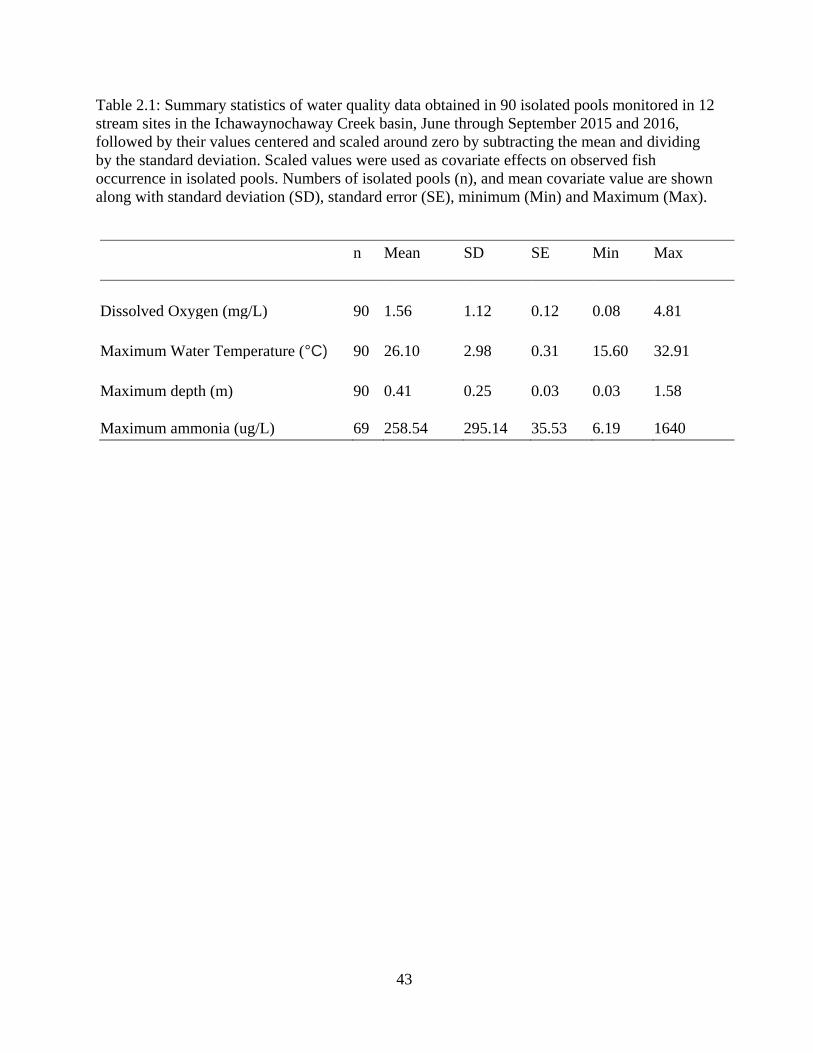
43
Table 2.1: Summary statistics of water quality data obtained in 90 isolated pools monitored in 12
stream sites in the Ichawaynochaway Creek basin, June through September 2015 and 2016,
followed by their values centered and scaled around zero by subtracting the mean and dividing
by the standard deviation. Scaled values were used as covariate effects on observed fish
occurrence in isolated pools. Numbers of isolated pools (n), and mean covariate value are shown
along with standard deviation (SD), standard error (SE), minimum (Min) and Maximum (Max).
n Mean SD SE Min Max
Dissolved Oxygen (mg/L) 90 1.56 1.12 0.12 0.08 4.81
Maximum Water Temperature (°C) 90 26.10 2.98 0.31 15.60 32.91
Maximum depth (m) 90 0.41 0.25 0.03 0.03 1.58
Maximum ammonia (ug/L) 69 258.54 295.14 35.53 6.19 1640
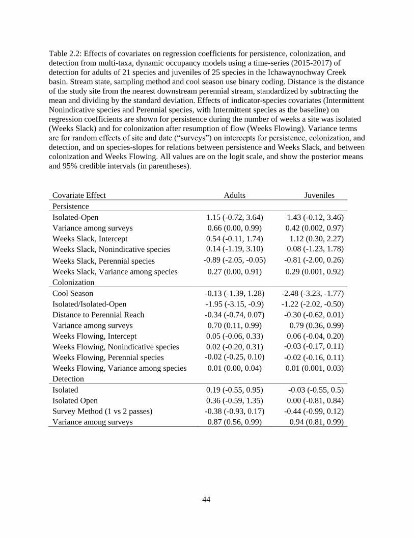
44
Table 2.2: Effects of covariates on regression coefficients for persistence, colonization, and
detection from multi-taxa, dynamic occupancy models using a time-series (2015-2017) of
detection for adults of 21 species and juveniles of 25 species in the Ichawaynochway Creek
basin. Stream state, sampling method and cool season use binary coding. Distance is the distance
of the study site from the nearest downstream perennial stream, standardized by subtracting the
mean and dividing by the standard deviation. Effects of indicator-species covariates (Intermittent
Nonindicative species and Perennial species, with Intermittent species as the baseline) on
regression coefficients are shown for persistence during the number of weeks a site was isolated
(Weeks Slack) and for colonization after resumption of flow (Weeks Flowing). Variance terms
are for random effects of site and date (“surveys”) on intercepts for persistence, colonization, and
detection, and on species-slopes for relations between persistence and Weeks Slack, and between
colonization and Weeks Flowing. All values are on the logit scale, and show the posterior means
and 95% credible intervals (in parentheses).
Covariate Effect Adults Juveniles
Persistence
Isolated-Open 1.15 (-0.72, 3.64) 1.43 (-0.12, 3.46)
Variance among surveys 0.66 (0.00, 0.99) 0.42 (0.002, 0.97)
Weeks Slack, Intercept 0.54 (-0.11, 1.74) 1.12 (0.30, 2.27)
Weeks Slack, Nonindicative species 0.14 (-1.19, 3.10) 0.08 (-1.23, 1.78)
Weeks Slack, Perennial species -0.89 (-2.05, -0.05) -0.81 (-2.00, 0.26)
Weeks Slack, Variance among species 0.27 (0.00, 0.91) 0.29 (0.001, 0.92)
Colonization
Cool Season -0.13 (-1.39, 1.28) -2.48 (-3.23, -1.77)
Isolated/Isolated-Open -1.95 (-3.15, -0.9) -1.22 (-2.02, -0.50)
Distance to Perennial Reach -0.34 (-0.74, 0.07) -0.30 (-0.62, 0.01)
Variance among surveys 0.70 (0.11, 0.99) 0.79 (0.36, 0.99)
Weeks Flowing, Intercept 0.05 (-0.06, 0.33) 0.06 (-0.04, 0.20)
Weeks Flowing, Nonindicative species 0.02 (-0.20, 0.31) -0.03 (-0.17, 0.11)
Weeks Flowing, Perennial species -0.02 (-0.25, 0.10) -0.02 (-0.16, 0.11)
Weeks Flowing, Variance among species 0.01 (0.00, 0.04) 0.01 (0.001, 0.03)
Detection
Isolated 0.19 (-0.55, 0.95) -0.03 (-0.55, 0.5)
Isolated Open 0.36 (-0.59, 1.35) 0.00 (-0.81, 0.84)
Survey Method (1 vs 2 passes) -0.38 (-0.93, 0.17) -0.44 (-0.99, 0.12)
Variance among surveys 0.87 (0.56, 0.99) 0.94 (0.81, 0.99)
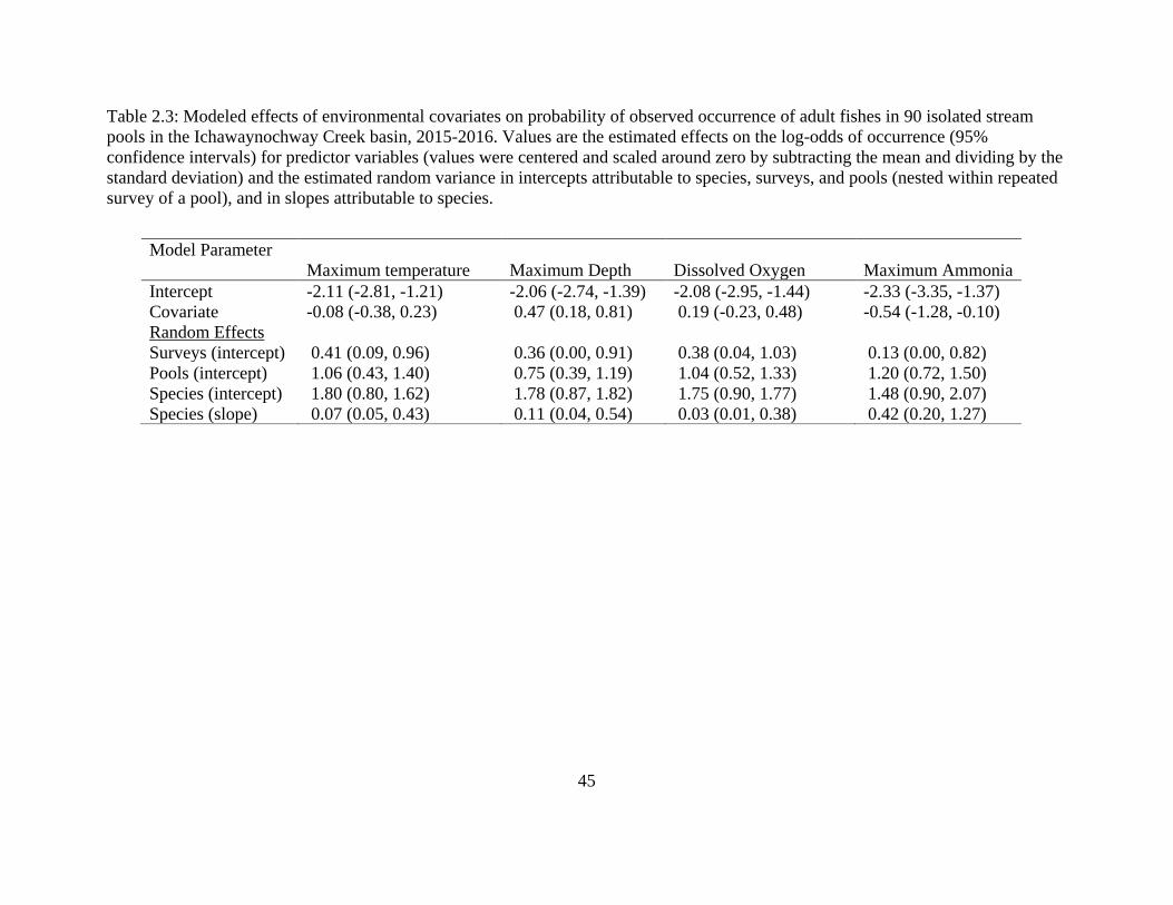
45
Table 2.3: Modeled effects of environmental covariates on probability of observed occurrence of adult fishes in 90 isolated stream
pools in the Ichawaynochway Creek basin, 2015-2016. Values are the estimated effects on the log-odds of occurrence (95%
confidence intervals) for predictor variables (values were centered and scaled around zero by subtracting the mean and dividing by the
standard deviation) and the estimated random variance in intercepts attributable to species, surveys, and pools (nested within repeated
survey of a pool), and in slopes attributable to species.
Model Parameter
Maximum temperature Maximum Depth Dissolved Oxygen Maximum Ammonia
Intercept -2.11 (-2.81, -1.21) -2.06 (-2.74, -1.39) -2.08 (-2.95, -1.44) -2.33 (-3.35, -1.37)
Covariate -0.08 (-0.38, 0.23) 0.47 (0.18, 0.81) 0.19 (-0.23, 0.48) -0.54 (-1.28, -0.10)
Random Effects
Surveys (intercept) 0.41 (0.09, 0.96) 0.36 (0.00, 0.91) 0.38 (0.04, 1.03) 0.13 (0.00, 0.82)
Pools (intercept) 1.06 (0.43, 1.40) 0.75 (0.39, 1.19) 1.04 (0.52, 1.33) 1.20 (0.72, 1.50)
Species (intercept) 1.80 (0.80, 1.62) 1.78 (0.87, 1.82) 1.75 (0.90, 1.77) 1.48 (0.90, 2.07)
Species (slope) 0.07 (0.05, 0.43) 0.11 (0.04, 0.54) 0.03 (0.01, 0.38) 0.42 (0.20, 1.27)
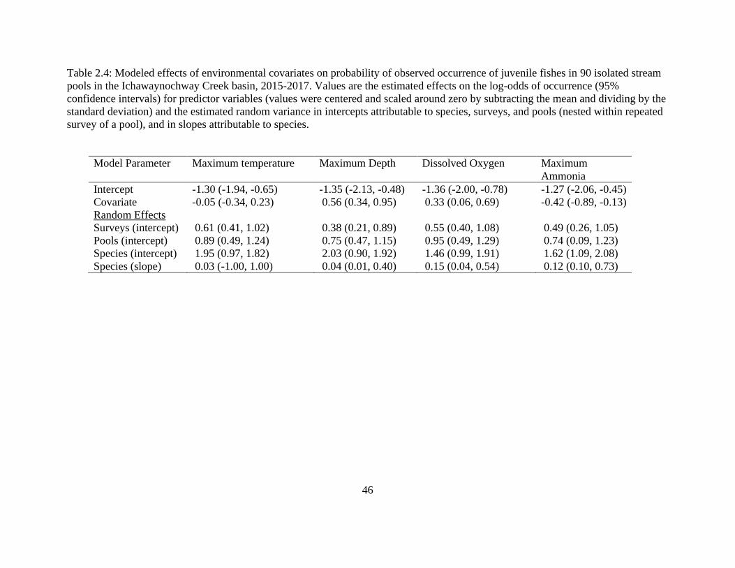
46
Table 2.4: Modeled effects of environmental covariates on probability of observed occurrence of juvenile fishes in 90 isolated stream
pools in the Ichawaynochway Creek basin, 2015-2017. Values are the estimated effects on the log-odds of occurrence (95%
confidence intervals) for predictor variables (values were centered and scaled around zero by subtracting the mean and dividing by the
standard deviation) and the estimated random variance in intercepts attributable to species, surveys, and pools (nested within repeated
survey of a pool), and in slopes attributable to species.
Model Parameter Maximum temperature Maximum Depth Dissolved Oxygen Maximum
Ammonia
Intercept -1.30 (-1.94, -0.65) -1.35 (-2.13, -0.48) -1.36 (-2.00, -0.78) -1.27 (-2.06, -0.45)
Covariate -0.05 (-0.34, 0.23) 0.56 (0.34, 0.95) 0.33 (0.06, 0.69) -0.42 (-0.89, -0.13)
Random Effects
Surveys (intercept) 0.61 (0.41, 1.02) 0.38 (0.21, 0.89) 0.55 (0.40, 1.08) 0.49 (0.26, 1.05)
Pools (intercept) 0.89 (0.49, 1.24) 0.75 (0.47, 1.15) 0.95 (0.49, 1.29) 0.74 (0.09, 1.23)
Species (intercept) 1.95 (0.97, 1.82) 2.03 (0.90, 1.92) 1.46 (0.99, 1.91) 1.62 (1.09, 2.08)
Species (slope) 0.03 (-1.00, 1.00) 0.04 (0.01, 0.40) 0.15 (0.04, 0.54) 0.12 (0.10, 0.73)
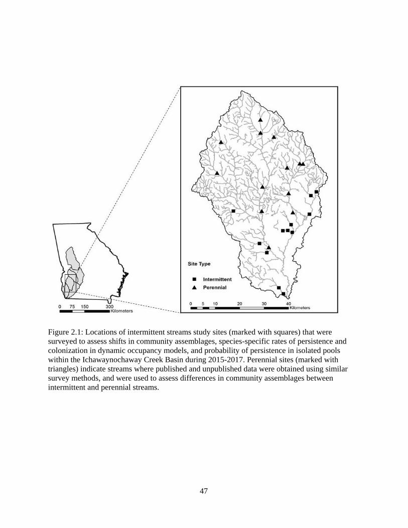
47
Figure 2.1: Locations of intermittent streams study sites (marked with squares) that were
surveyed to assess shifts in community assemblages, species-specific rates of persistence and
colonization in dynamic occupancy models, and probability of persistence in isolated pools
within the Ichawaynochaway Creek Basin during 2015-2017. Perennial sites (marked with
triangles) indicate streams where published and unpublished data were obtained using similar
survey methods, and were used to assess differences in community assemblages between
intermittent and perennial streams.

48
Figure 2.2: Discharge, water temperature, and air temperature at Spring Creek near Leary, GA (USGS gage 02354475). Periods where
discharge is at or near zero represent timing of intermittency, during which isolation or complete drying occurred.
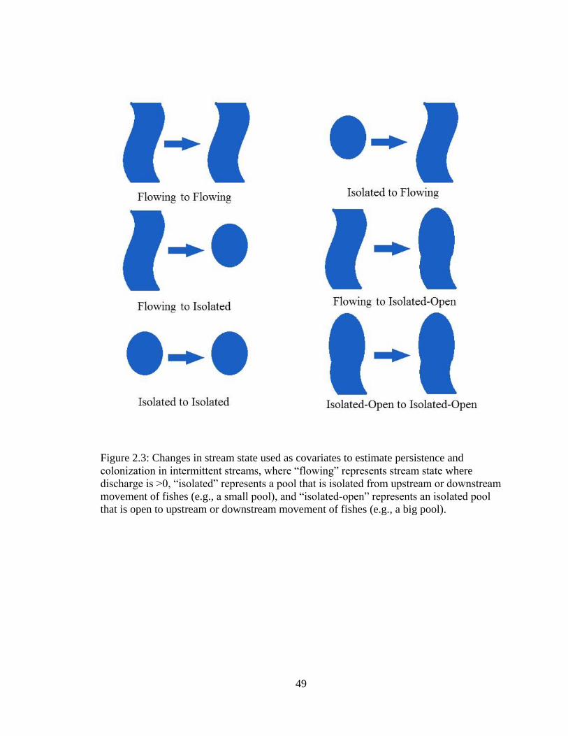
49
Figure 2.3: Changes in stream state used as covariates to estimate persistence and
colonization in intermittent streams, where “flowing” represents stream state where
discharge is >0, “isolated” represents a pool that is isolated from upstream or downstream
movement of fishes (e.g., a small pool), and “isolated-open” represents an isolated pool
that is open to upstream or downstream movement of fishes (e.g., a big pool).
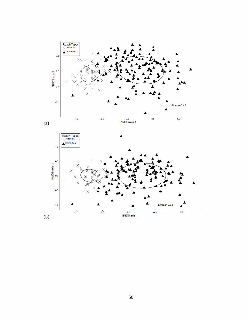
50
(a)
(b)
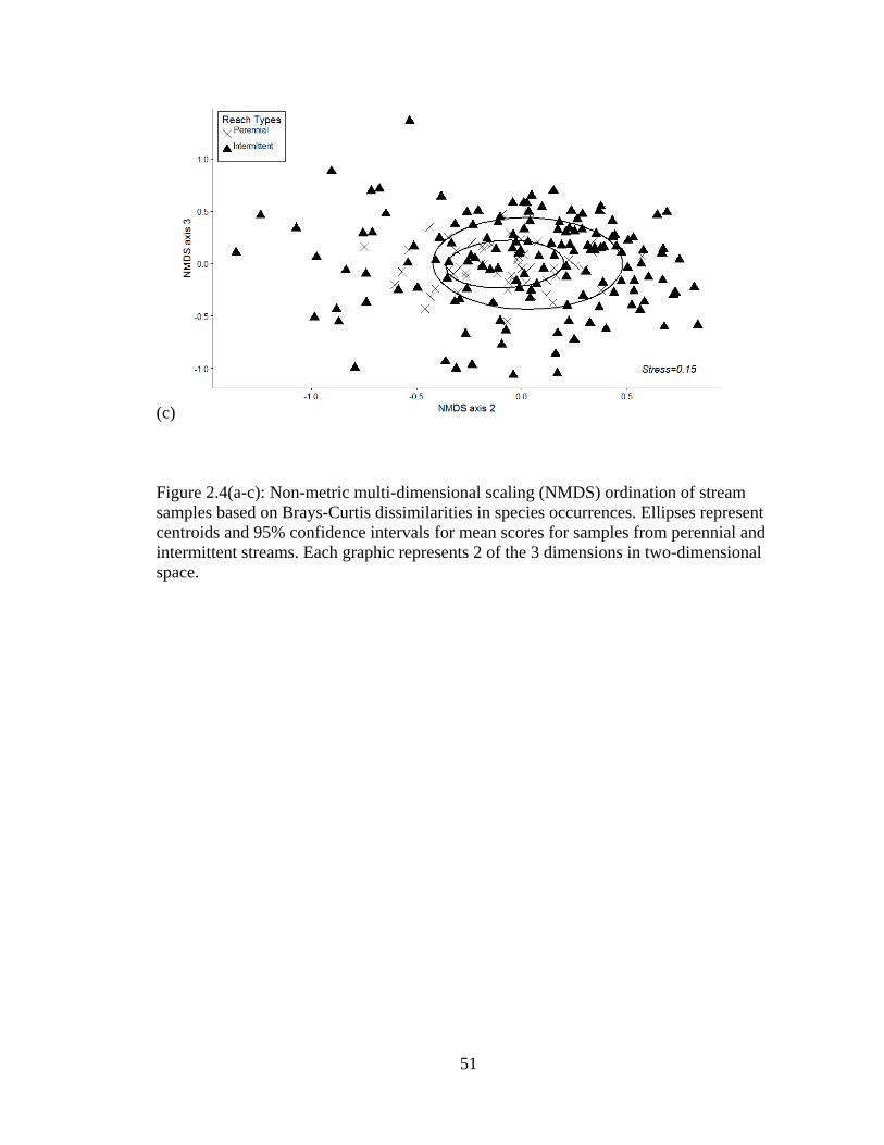
51
(c)
Figure 2.4(a-c): Non-metric multi-dimensional scaling (NMDS) ordination of stream
samples based on Brays-Curtis dissimilarities in species occurrences. Ellipses represent
centroids and 95% confidence intervals for mean scores for samples from perennial and
intermittent streams. Each graphic represents 2 of the 3 dimensions in two-dimensional
space.
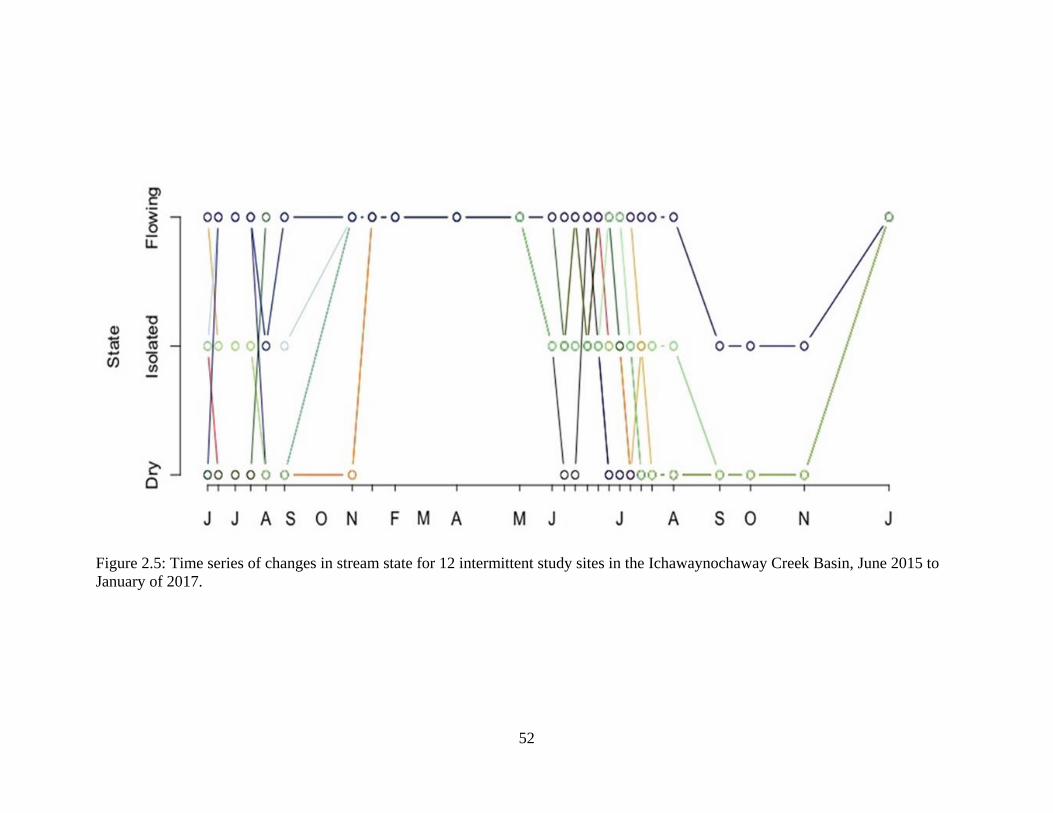
52
Figure 2.5: Time series of changes in stream state for 12 intermittent study sites in the Ichawaynochaway Creek Basin, June 2015 to
January of 2017.
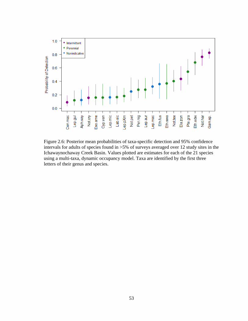
53
Figure 2.6: Posterior mean probabilities of taxa-specific detection and 95% confidence
intervals for adults of species found in >5% of surveys averaged over 12 study sites in the
Ichawaynochaway Creek Basin. Values plotted are estimates for each of the 21 species
using a multi-taxa, dynamic occupancy model. Taxa are identified by the first three
letters of their genus and species.
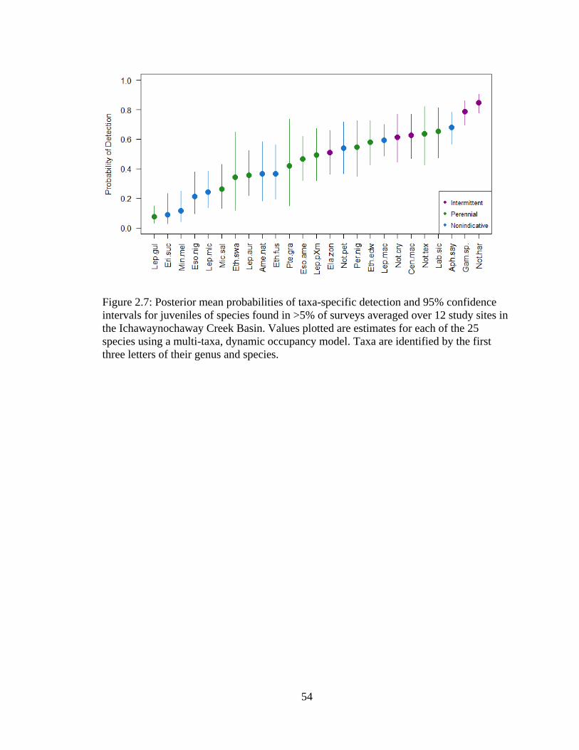
54
Figure 2.7: Posterior mean probabilities of taxa-specific detection and 95% confidence
intervals for juveniles of species found in >5% of surveys averaged over 12 study sites in
the Ichawaynochaway Creek Basin. Values plotted are estimates for each of the 25
species using a multi-taxa, dynamic occupancy model. Taxa are identified by the first
three letters of their genus and species.
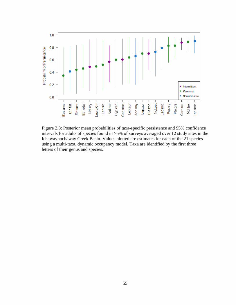
55
Figure 2.8: Posterior mean probabilities of taxa-specific persistence and 95% confidence
intervals for adults of species found in >5% of surveys averaged over 12 study sites in the
Ichawaynochaway Creek Basin. Values plotted are estimates for each of the 21 species
using a multi-taxa, dynamic occupancy model. Taxa are identified by the first three
letters of their genus and species.
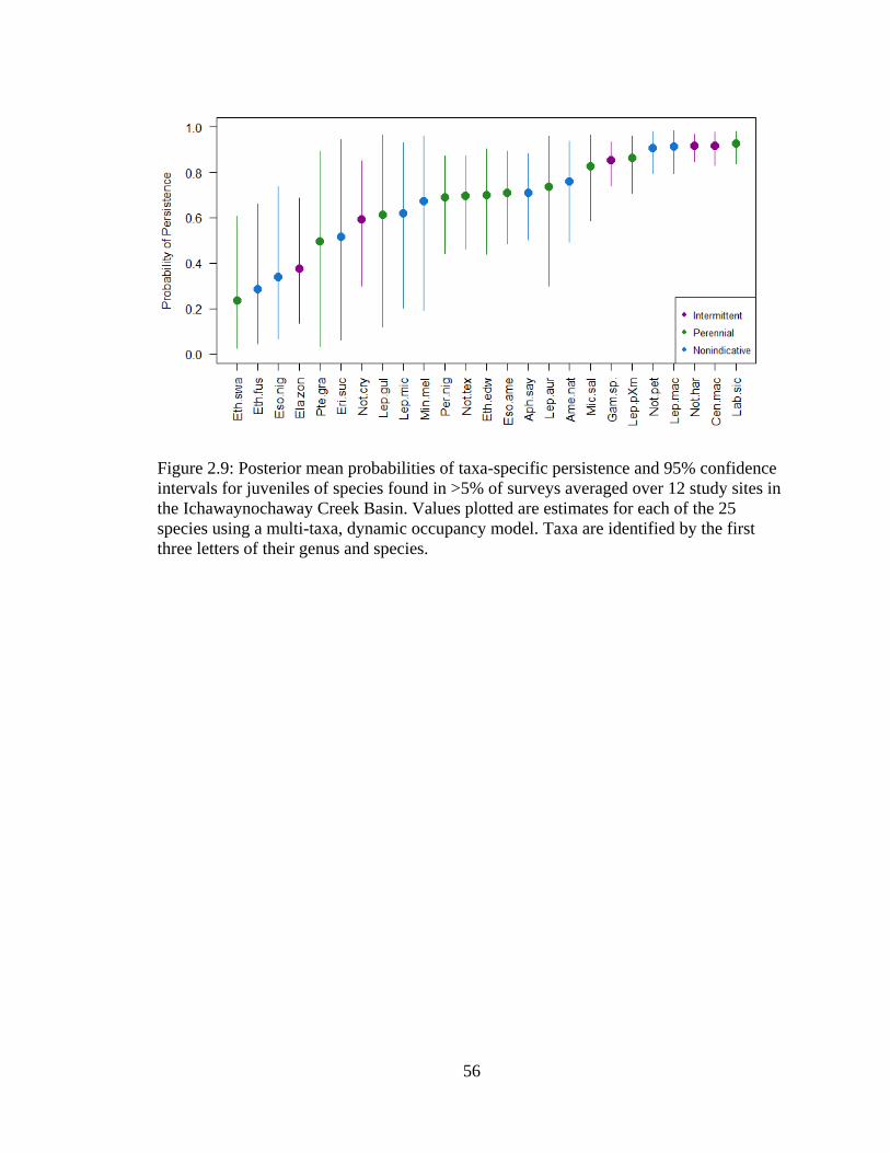
56
Figure 2.9: Posterior mean probabilities of taxa-specific persistence and 95% confidence
intervals for juveniles of species found in >5% of surveys averaged over 12 study sites in
the Ichawaynochaway Creek Basin. Values plotted are estimates for each of the 25
species using a multi-taxa, dynamic occupancy model. Taxa are identified by the first
three letters of their genus and species.
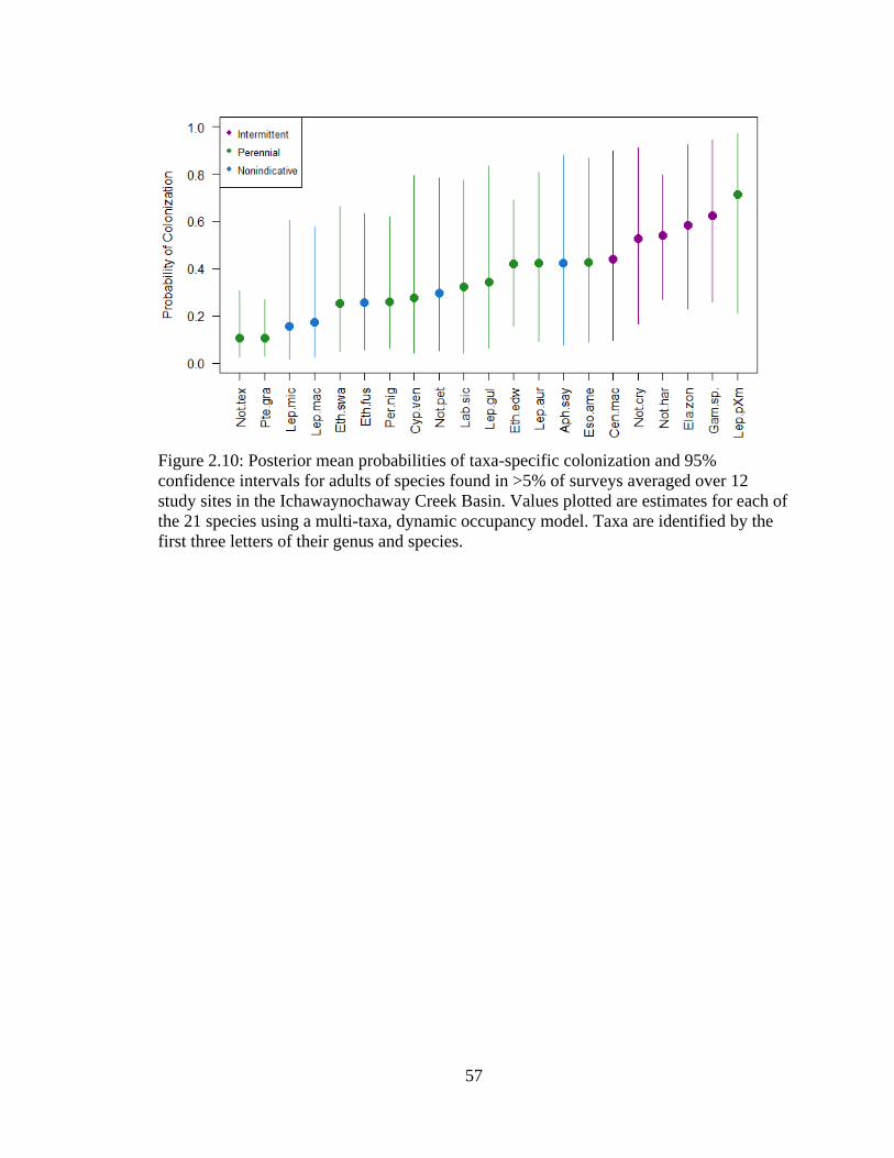
57
Figure 2.10: Posterior mean probabilities of taxa-specific colonization and 95%
confidence intervals for adults of species found in >5% of surveys averaged over 12
study sites in the Ichawaynochaway Creek Basin. Values plotted are estimates for each of
the 21 species using a multi-taxa, dynamic occupancy model. Taxa are identified by the
first three letters of their genus and species.
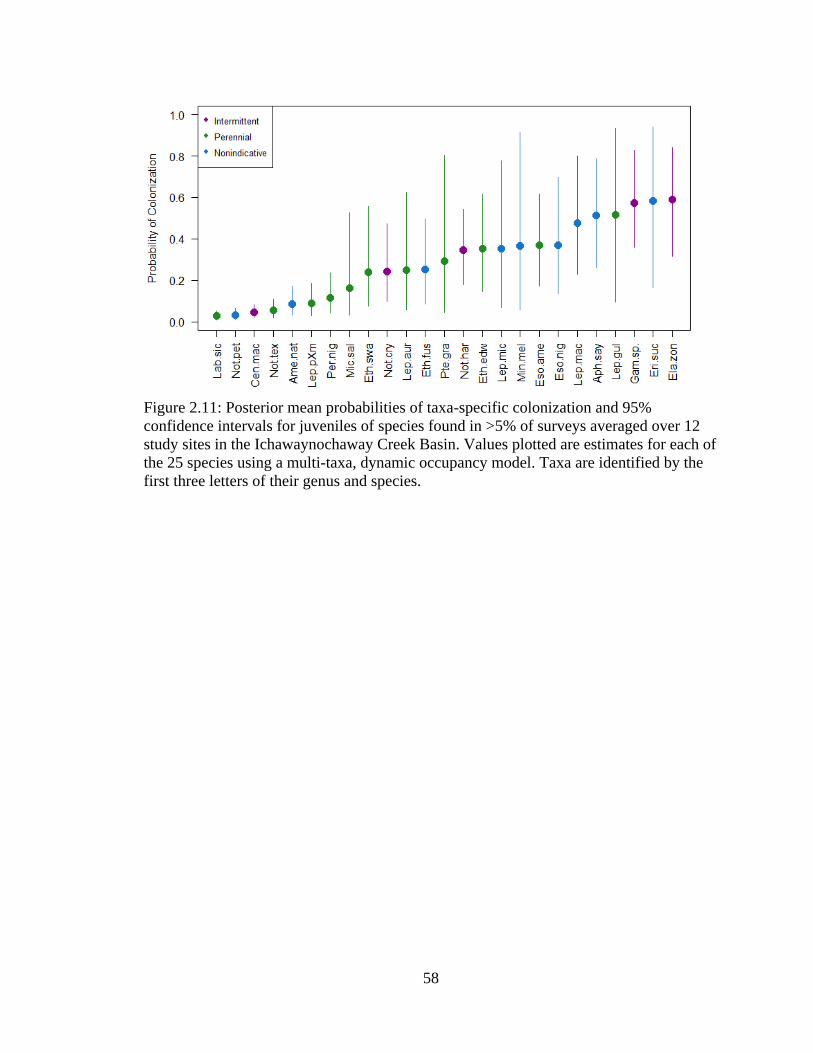
58
Figure 2.11: Posterior mean probabilities of taxa-specific colonization and 95%
confidence intervals for juveniles of species found in >5% of surveys averaged over 12
study sites in the Ichawaynochaway Creek Basin. Values plotted are estimates for each of
the 25 species using a multi-taxa, dynamic occupancy model. Taxa are identified by the
first three letters of their genus and species.
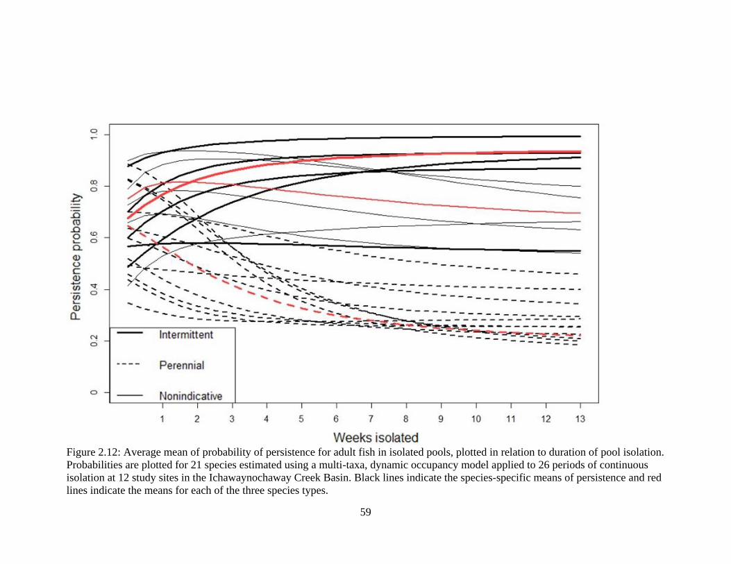
59
Figure 2.12: Average mean of probability of persistence for adult fish in isolated pools, plotted in relation to duration of pool isolation.
Probabilities are plotted for 21 species estimated using a multi-taxa, dynamic occupancy model applied to 26 periods of continuous
isolation at 12 study sites in the Ichawaynochaway Creek Basin. Black lines indicate the species-specific means of persistence and red
lines indicate the means for each of the three species types.
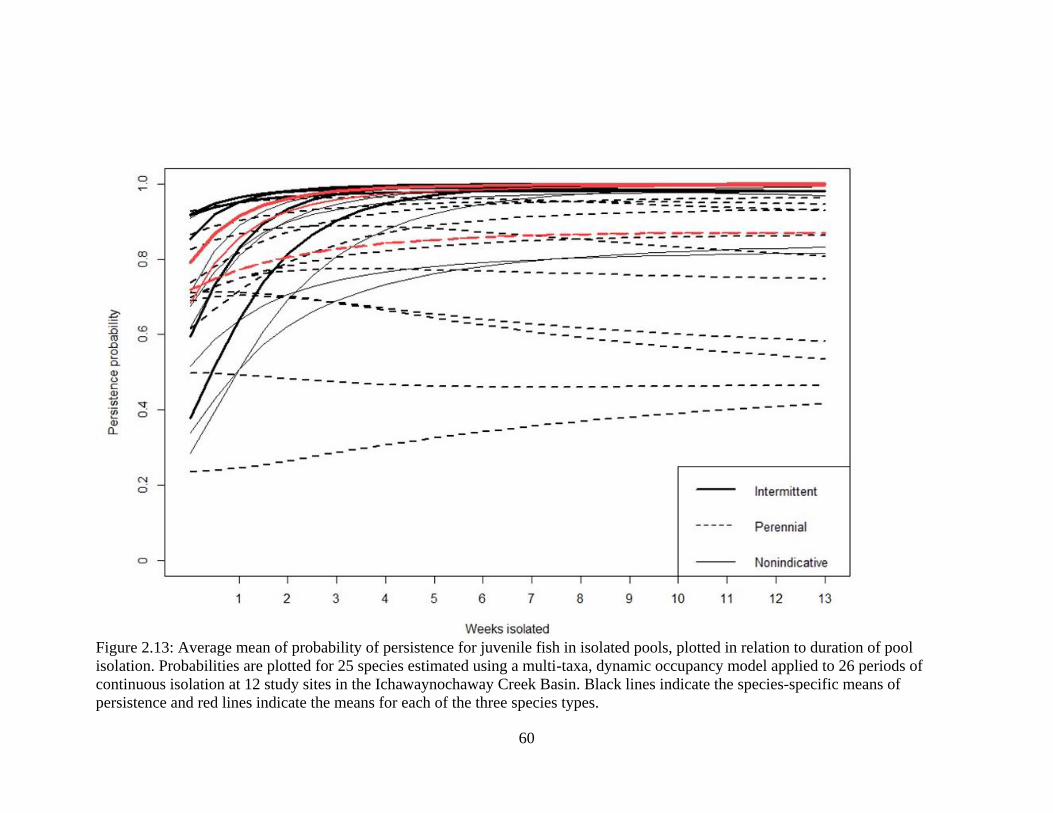
60
Figure 2.13: Average mean of probability of persistence for juvenile fish in isolated pools, plotted in relation to duration of pool
isolation. Probabilities are plotted for 25 species estimated using a multi-taxa, dynamic occupancy model applied to 26 periods of
continuous isolation at 12 study sites in the Ichawaynochaway Creek Basin. Black lines indicate the species-specific means of
persistence and red lines indicate the means for each of the three species types.
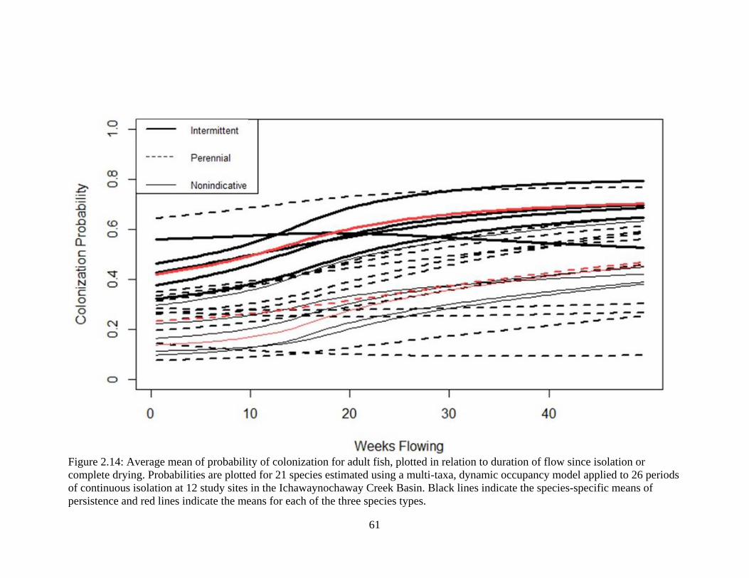
61
Figure 2.14: Average mean of probability of colonization for adult fish, plotted in relation to duration of flow since isolation or
complete drying. Probabilities are plotted for 21 species estimated using a multi-taxa, dynamic occupancy model applied to 26 periods
of continuous isolation at 12 study sites in the Ichawaynochaway Creek Basin. Black lines indicate the species-specific means of
persistence and red lines indicate the means for each of the three species types.

62
Figure 2.15: Average mean of probability of colonization for juvenile fish, plotted in relation to duration of flow since isolation or
complete drying. Probabilities are plotted for 25 species estimated using a multi-taxa, dynamic occupancy model applied to 26 periods
of continuous isolation at 12 study sites in the Ichawaynochaway Creek Basin. Black lines indicate the species-specific means of
persistence and red lines indicate the means for each of the three species types.
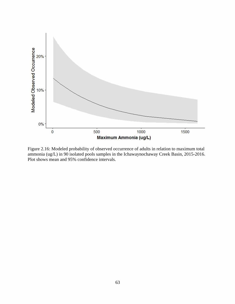
63
Figure 2.16: Modeled probability of observed occurrence of adults in relation to maximum total
ammonia (ug/L) in 90 isolated pools samples in the Ichawaynochaway Creek Basin, 2015-2016.
Plot shows mean and 95% confidence intervals.
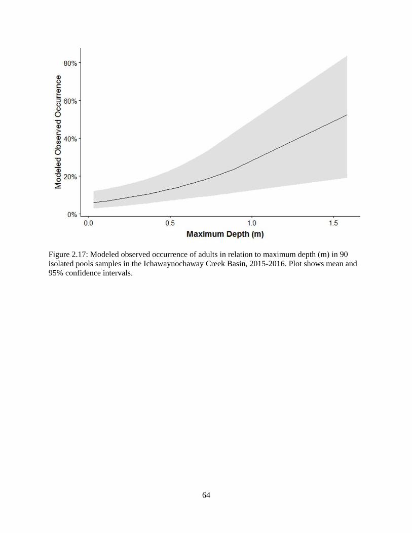
64
Figure 2.17: Modeled observed occurrence of adults in relation to maximum depth (m) in 90
isolated pools samples in the Ichawaynochaway Creek Basin, 2015-2016. Plot shows mean and
95% confidence intervals.
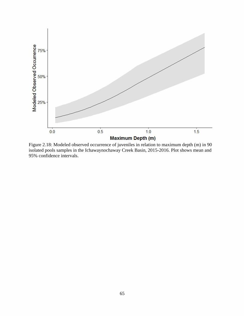
65
Figure 2.18: Modeled observed occurrence of juveniles in relation to maximum depth (m) in 90
isolated pools samples in the Ichawaynochaway Creek Basin, 2015-2016. Plot shows mean and
95% confidence intervals.
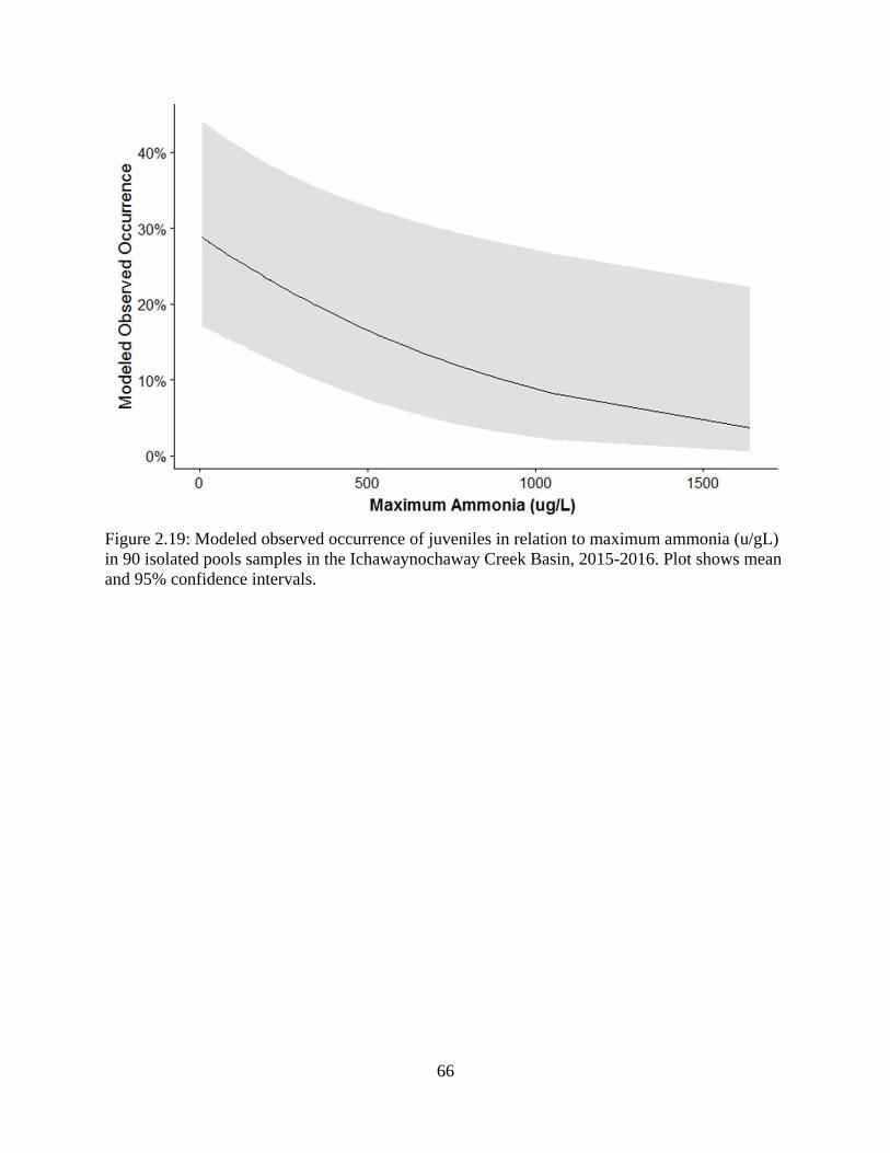
66
Figure 2.19: Modeled observed occurrence of juveniles in relation to maximum ammonia (u/gL)
in 90 isolated pools samples in the Ichawaynochaway Creek Basin, 2015-2016. Plot shows mean
and 95% confidence intervals.
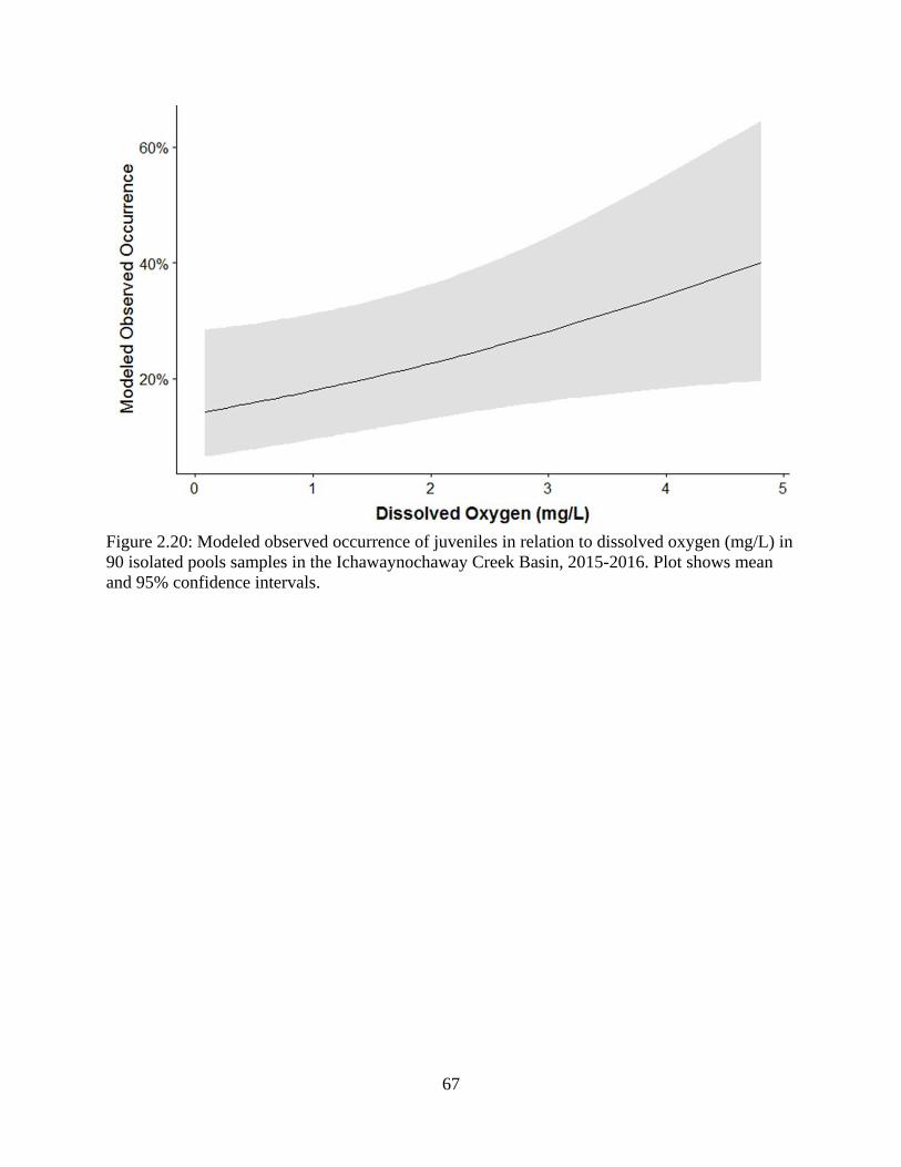
67
Figure 2.20: Modeled observed occurrence of juveniles in relation to dissolved oxygen (mg/L) in
90 isolated pools samples in the Ichawaynochaway Creek Basin, 2015-2016. Plot shows mean
and 95% confidence intervals.
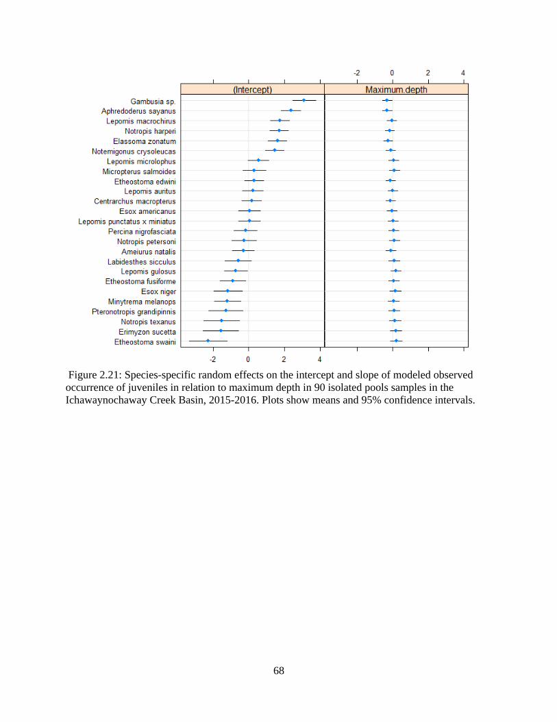
68
Figure 2.21: Species-specific random effects on the intercept and slope of modeled observed
occurrence of juveniles in relation to maximum depth in 90 isolated pools samples in the
Ichawaynochaway Creek Basin, 2015-2016. Plots show means and 95% confidence intervals.
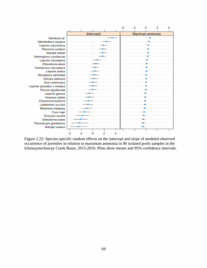
69
Figure 2.22: Species-specific random effects on the intercept and slope of modeled observed
occurrence of juveniles in relation to maximum ammonia in 90 isolated pools samples in the
Ichawaynochaway Creek Basin, 2015-2016. Plots show means and 95% confidence intervals.
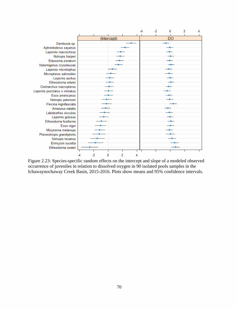
70
Figure 2.23: Species-specific random effects on the intercept and slope of a modeled observed
occurrence of juveniles in relation to dissolved oxygen in 90 isolated pools samples in the
Ichawaynochaway Creek Basin, 2015-2016. Plots show means and 95% confidence intervals.
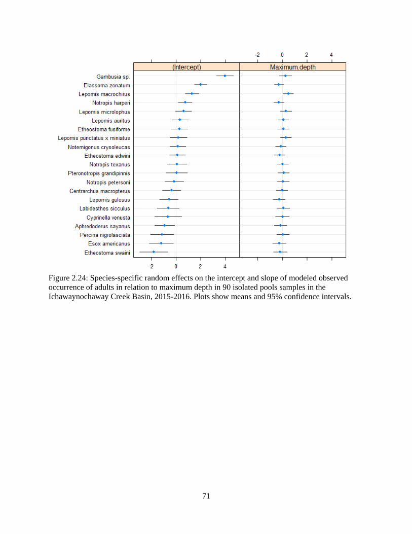
71
Figure 2.24: Species-specific random effects on the intercept and slope of modeled observed
occurrence of adults in relation to maximum depth in 90 isolated pools samples in the
Ichawaynochaway Creek Basin, 2015-2016. Plots show means and 95% confidence intervals.
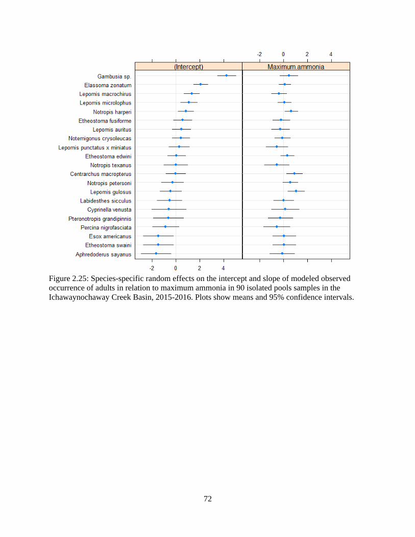
72
Figure 2.25: Species-specific random effects on the intercept and slope of modeled observed
occurrence of adults in relation to maximum ammonia in 90 isolated pools samples in the
Ichawaynochaway Creek Basin, 2015-2016. Plots show means and 95% confidence intervals.

1Davis, J. L., M. C. Freeman, S. W. Golladay. To be submitted to Freshwater Biology
CHAPTER 3
IDENTIFYING LIFE HISTORY TRAITS THAT PROMOTE FISH SPECIES PERSISTENCE
IN INTERMITTENT STREAMS1
73
74
Abstract
Life history traits of stream fishes partly reflect adaptations to natural flow regimes,
which in turn shape assemblage composition via environmental filtering on species persistence.
Thus, trait-based approaches, including the trilateral life history model, have been useful for
understanding species responses to streamflow alteration. In this study, I focused on life history
traits of four cyprinid species in a Coastal Plain stream system of southwestern GA that is
shifting from historically perennial streamflow to intermittency. Native fishes, including these
four species, vary in occurrence, and tolerance to intermittency. I evaluated differences among
the four cyprinids in reproductive timing (based on ovary and oocyte development), sex ratio,
body size at maturity, and reproductive investment (gonadosomatic index (GSI), gonad weight
and egg diameter), traits hypothesized to influence the ability of species to persist in intermittent
streams. I periodically sampled individuals in 14 streams over the duration of a year (May 2016-
April 2017). I found that for Notropis harperi, a species with high persistence rates, reproductive
timing did not overlap with typical seasonal stream drying. N. harperi also had the significantly
smallest minimum length at maturation, greatest GSI and gonad weight, and a tendency towards
larger average egg diameter. Species with low persistence rates in isolated pools (Notropis
petersoni, Notropis texanus, and Pteronotropis grandipinnis), had at least a portion of their
reproductive timing overlapping with times when streams were likely to dry, and had
significantly lower GSI and relative gonad weight than N. harperi. All four species would be
considered opportunistic, rather than periodic or equilibrium, strategists. Our results suggest
however, that some life history traits used to define the trilateral life history model may be useful
for understanding differences in how even closely related species respond to changing

75
environments, with smaller body size at maturity along with appropriate reproductive timing
promoting greater persistence given more frequent and intense periods of drying.
76
Introduction
Streamflow defines the physical template of river ecosystems (Poff 1997) and acts as a
selective force and an ecological filter for survival strategies of aquatic organisms (Townsend
and Hildrew 1994, Lytle and Poff 2004). It shapes the distribution and character of riverine
habitats and, in turn, the distribution and abundance of lotic organisms (Power et al. 1995, Bunn
and Arthington 2002). Species adaptations to flow regime occur as a response to the interaction
between frequency, magnitude, and predictability of mortality-causing events (Lytle and Poff
2004). Streamflow in lotic systems has been altered by humans for many reasons, including
extraction for water supply, impoundments for flood control and hydropower, and to support
irrigated agriculture. Human freshwater needs and actions have altered historical hydrologic
regimes, reducing effectiveness of some biotic adaptations, and decreasing stream suitability for
native fauna (Pringle et al. 2000).
Increasingly, species traits are being used to study flow-ecology relationships across
diverse species-assemblages and broad geographic scales (Poff et al. 2006, Frimpong and
Angermeier 2010). Life-history theory predicts that the magnitude, frequency, and predictability
of hydrologic events, such as floods or droughts, can affect evolutionary processes (Iwasa and
Levin 1995, Lytle and Poff 2004). Convergence in the suites of traits characterizing dominant
species along hydrologic gradients has been demonstrated for freshwater fishes (Lamouroux et
al. 2002, Logez et al. 2010), and studies testing predictions from life-history theory support these
relationships (Tedesco et al. 2008, Kennard et al. 2010, Carlisle et al. 2011). This developing
body of work has provided insights into environmental influences on community assemblages in
fresh waters (Poff and Allan 1995, McManamay and Frimpong 2015) and provides useful

77
frameworks for developing flow-ecology hypotheses and environmental flow standards
(McManamay et al. 2015).
Environmental variability is a natural part of aquatic ecosystems and influences the
structure of aquatic communities (Resh et al. 1988, Poff and Allan 1995). From an evolutionary
perspective, floods and droughts that are relatively predictable in their frequency, duration, and
intensity can exert selective pressures that filter certain life history traits, while on ecological
time scales, flow regime shapes assemblage composition by altering population numbers and
species persistence (Poff 1997, Naiman et al. 2008). In systems with a high degree of flow
variability (i.e., hydrologically ‘flashy’) including intermittence, fish assemblages are controlled
by abiotic factors (Echelle et al. 1972, Taylor 1997, Matthews and Marsh-Matthews 2003). As a
result, the predominant fish species in these systems are especially tolerant of variable
environmental conditions ( Winemiller 1989, Fausch and Bramblett 1991).
While drought and stream intermittency are normal processes, low-flow and no-flow
events are increasing in frequency in many areas due to anthropogenic alterations of streamflow
regimes through dams, water diversion, and climate shifts (Brown et al. 2013). The ecological
effects of low-flows are expected to accumulate with increasing frequency and duration (Lake
2003). Evidence suggests that climate-driven streamflow intermittence has increased in the
southeastern US (Palmer et al. 2008b, Falke et al. 2011), including the Coastal Plain of Georgia,
where trends in declining seasonal flows are projected to continue (Larned et al. 2010, Golladay
and Hicks 2013). Natural resource managers face the challenge of understanding the effects of
both water withdrawals, and projected increases in intermittency, when working towards
conserving biological integrity of freshwater systems. Management can be improved through
models of fish responses to low-flow or isolated events that account for life history traits.
78
Life history theory proposes that populations are regulated by trade-offs along
demographic axes of age at maturity, juvenile survival, and fecundity (Stearns 1977). The
trilateral life history model proposed by Winemiller and Rose (1992) identifies three life history
strategies for fishes using tradeoffs among basic demographic parameters. The endpoints of the
trilateral life history model represent strategies that are optimal under certain environmental
conditions (Winemiller and Rose 1992, Winemiller 2005). Opportunistic Strategists (OS) are
predicted to be associated with habitats defined by frequent and intense disturbances. OS have
short generation time, high fecundity, and low juvenile survivorship. Periodic Strategists (PS) are
favored under predictable yet seasonally fluctuating environments. PS maximize fecundity via
delayed reproduction and have larger maturation size. Equilibrium Strategists (ES) are favored
under stable environmental conditions. ES maximize juvenile survival through low fecundity per
spawning event, have larger eggs, and prolonged parental care. Studies have found utility in fish
life-history trait ordination along these three axes across North America (Kennard et al. 2010,
Mims et al. 2010, Mims and Olden 2013, Perkin et al. 2017) for predicting responses to natural
and altered flow regimes on fish assemblages. For example, a study of two cyprinid and one
percid species shows PS traits (high fecundity) favored at sites with greater flow seasonality and
low variability, while ES traits (large eggs) were prevalent in stable flow conditions (Bennett et
al. 2016). Nevertheless, intraspecific trait variation may contradict the trilateral life history
model (Bennett et al. 2016). Additionally, species placement within the trilateral life history
model is largely dependent on the species assessed within an assemblage.
This study focused on four commonly occurring, yet relatively understudied cyprinid
species, Pteronotropis grandipinnis, Notropis harperi, Notropis petersoni, and Notropis texanus,
in a southeastern Coastal Plain system. I previously found that mature individuals of these
79
cyprinid taxa vary substantially in rates of persistence during periods of flow intermittence, when
fishes are restricted to isolated pools, yet the underlying life history mechanisms remain
unknown (Chapter two of this thesis, Figure 3.1). Regional streamflows in my study area are
strongly influenced by agricultural water withdrawals and climate variability, resulting in
increases in the duration and intensity of intermittency. The primary objective of this study was
to explore life history strategies that enable cyprinid species to persist within intermittent streams
and to determine if those life history traits actually coincide with high persistence rates. I
explored differences in reproductive timing, sex ratio, reproductive size, reproductive investment
(via gonadosomatic index (GSI), gonad weight, egg diameter), and food habits during flowing
and intermittent periods. A secondary objective was to determine if predictions of the trilateral
life history model apply to morphologically similar species belonging to a single family. I
hypothesized that (i) species with low persistence probabilities reproduce during summer months
(e.g., when periods of stream drying to isolated pools occur); (ii) species with high persistence
probabilities have increased reproductive investment as assessed via GSI, gonad weight, and egg
diameter; (iii) higher probabilities of persistence (N. harperi) coincides with OS, low
probabilities of persistence (N. texanus and P. grandipinnis) coincides with ES, and intermediate
probabilities of persistence (N. petersoni) coincides with PS; and (iv) species with higher
persistence will have a greater shift in diet items between flowing and intermittent periods,
reflecting intentional feeding patterns while streams flow and more opportunistic feeding
patterns during intermittence.
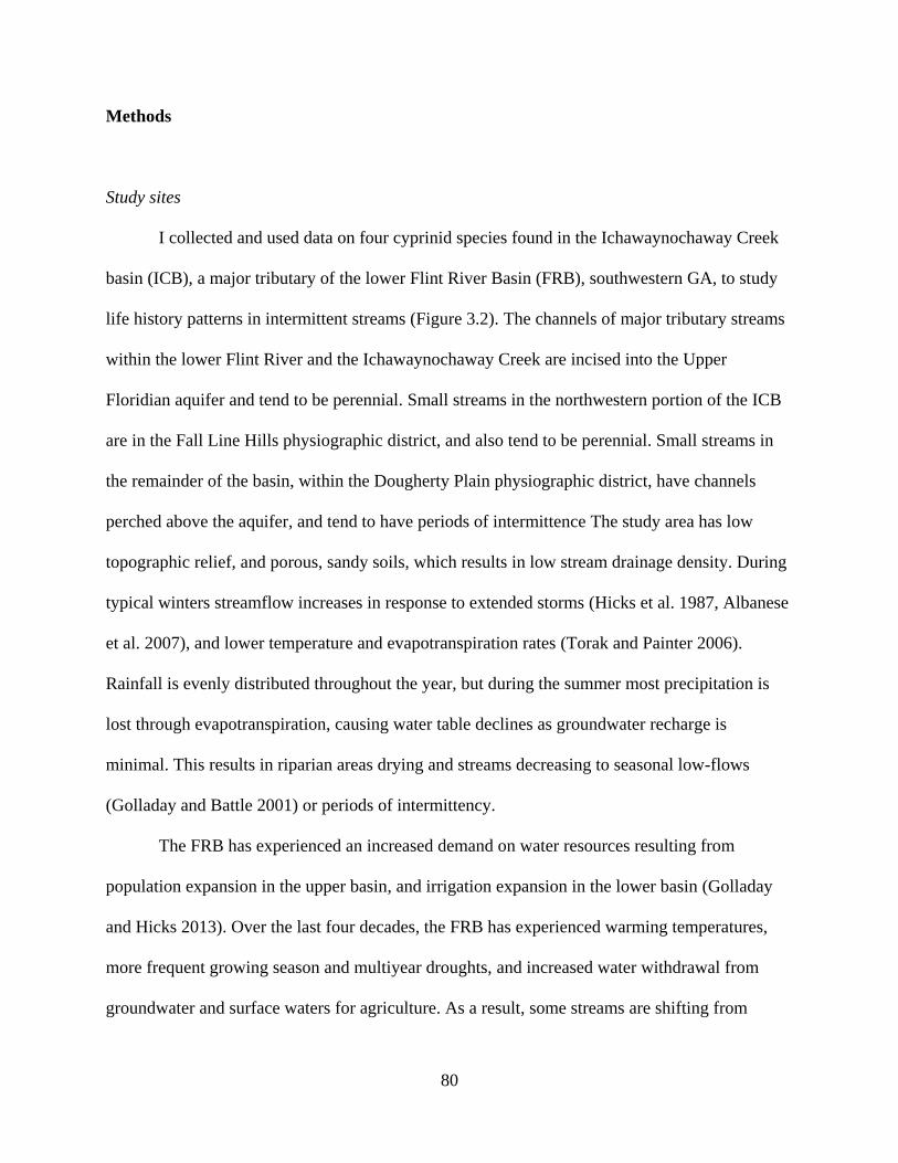
80
Methods
Study sites
I collected and used data on four cyprinid species found in the Ichawaynochaway Creek
basin (ICB), a major tributary of the lower Flint River Basin (FRB), southwestern GA, to study
life history patterns in intermittent streams (Figure 3.2). The channels of major tributary streams
within the lower Flint River and the Ichawaynochaway Creek are incised into the Upper
Floridian aquifer and tend to be perennial. Small streams in the northwestern portion of the ICB
are in the Fall Line Hills physiographic district, and also tend to be perennial. Small streams in
the remainder of the basin, within the Dougherty Plain physiographic district, have channels
perched above the aquifer, and tend to have periods of intermittence The study area has low
topographic relief, and porous, sandy soils, which results in low stream drainage density. During
typical winters streamflow increases in response to extended storms (Hicks et al. 1987, Albanese
et al. 2007), and lower temperature and evapotranspiration rates (Torak and Painter 2006).
Rainfall is evenly distributed throughout the year, but during the summer most precipitation is
lost through evapotranspiration, causing water table declines as groundwater recharge is
minimal. This results in riparian areas drying and streams decreasing to seasonal low-flows
(Golladay and Battle 2001) or periods of intermittency.
The FRB has experienced an increased demand on water resources resulting from
population expansion in the upper basin, and irrigation expansion in the lower basin (Golladay
and Hicks 2013). Over the last four decades, the FRB has experienced warming temperatures,
more frequent growing season and multiyear droughts, and increased water withdrawal from
groundwater and surface waters for agriculture. As a result, some streams are shifting from
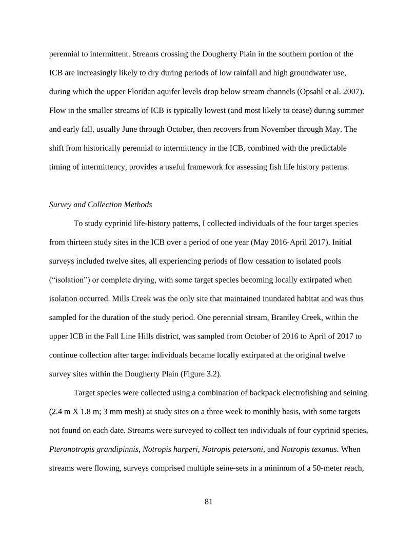
81
perennial to intermittent. Streams crossing the Dougherty Plain in the southern portion of the
ICB are increasingly likely to dry during periods of low rainfall and high groundwater use,
during which the upper Floridan aquifer levels drop below stream channels (Opsahl et al. 2007).
Flow in the smaller streams of ICB is typically lowest (and most likely to cease) during summer
and early fall, usually June through October, then recovers from November through May. The
shift from historically perennial to intermittency in the ICB, combined with the predictable
timing of intermittency, provides a useful framework for assessing fish life history patterns.
Survey and Collection Methods
To study cyprinid life-history patterns, I collected individuals of the four target species
from thirteen study sites in the ICB over a period of one year (May 2016-April 2017). Initial
surveys included twelve sites, all experiencing periods of flow cessation to isolated pools
(“isolation”) or complete drying, with some target species becoming locally extirpated when
isolation occurred. Mills Creek was the only site that maintained inundated habitat and was thus
sampled for the duration of the study period. One perennial stream, Brantley Creek, within the
upper ICB in the Fall Line Hills district, was sampled from October of 2016 to April of 2017 to
continue collection after target individuals became locally extirpated at the original twelve
survey sites within the Dougherty Plain (Figure 3.2).
Target species were collected using a combination of backpack electrofishing and seining
(2.4 m X 1.8 m; 3 mm mesh) at study sites on a three week to monthly basis, with some targets
not found on each date. Streams were surveyed to collect ten individuals of four cyprinid species,
Pteronotropis grandipinnis, Notropis harperi, Notropis petersoni, and Notropis texanus. When
streams were flowing, surveys comprised multiple seine-sets in a minimum of a 50-meter reach,
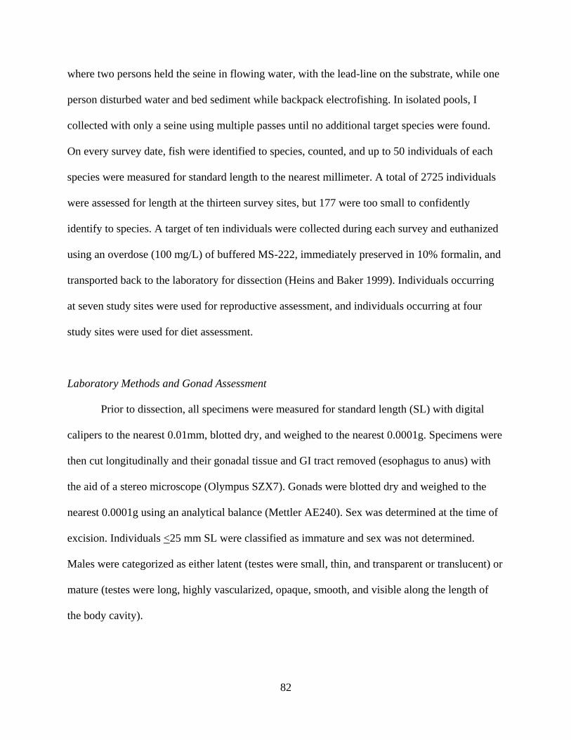
82
where two persons held the seine in flowing water, with the lead-line on the substrate, while one
person disturbed water and bed sediment while backpack electrofishing. In isolated pools, I
collected with only a seine using multiple passes until no additional target species were found.
On every survey date, fish were identified to species, counted, and up to 50 individuals of each
species were measured for standard length to the nearest millimeter. A total of 2725 individuals
were assessed for length at the thirteen survey sites, but 177 were too small to confidently
identify to species. A target of ten individuals were collected during each survey and euthanized
using an overdose (100 mg/L) of buffered MS-222, immediately preserved in 10% formalin, and
transported back to the laboratory for dissection (Heins and Baker 1999). Individuals occurring
at seven study sites were used for reproductive assessment, and individuals occurring at four
study sites were used for diet assessment.
Laboratory Methods and Gonad Assessment
Prior to dissection, all specimens were measured for standard length (SL) with digital
calipers to the nearest 0.01mm, blotted dry, and weighed to the nearest 0.0001g. Specimens were
then cut longitudinally and their gonadal tissue and GI tract removed (esophagus to anus) with
the aid of a stereo microscope (Olympus SZX7). Gonads were blotted dry and weighed to the
nearest 0.0001g using an analytical balance (Mettler AE240). Sex was determined at the time of
excision. Individuals <25 mm SL were classified as immature and sex was not determined.
Males were categorized as either latent (testes were small, thin, and transparent or translucent) or
mature (testes were long, highly vascularized, opaque, smooth, and visible along the length of
the body cavity).
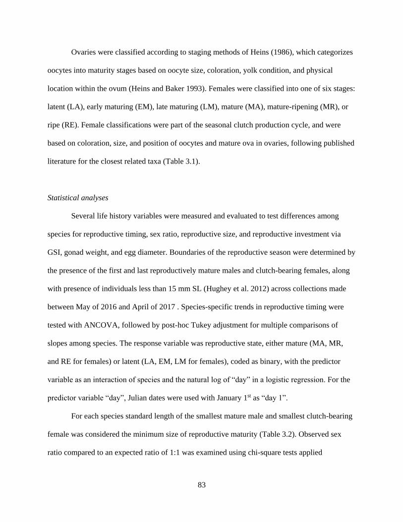
83
Ovaries were classified according to staging methods of Heins (1986), which categorizes
oocytes into maturity stages based on oocyte size, coloration, yolk condition, and physical
location within the ovum (Heins and Baker 1993). Females were classified into one of six stages:
latent (LA), early maturing (EM), late maturing (LM), mature (MA), mature-ripening (MR), or
ripe (RE). Female classifications were part of the seasonal clutch production cycle, and were
based on coloration, size, and position of oocytes and mature ova in ovaries, following published
literature for the closest related taxa (Table 3.1).
Statistical analyses
Several life history variables were measured and evaluated to test differences among
species for reproductive timing, sex ratio, reproductive size, and reproductive investment via
GSI, gonad weight, and egg diameter. Boundaries of the reproductive season were determined by
the presence of the first and last reproductively mature males and clutch-bearing females, along
with presence of individuals less than 15 mm SL (Hughey et al. 2012) across collections made
between May of 2016 and April of 2017 . Species-specific trends in reproductive timing were
tested with ANCOVA, followed by post-hoc Tukey adjustment for multiple comparisons of
slopes among species. The response variable was reproductive state, either mature (MA, MR,
and RE for females) or latent (LA, EM, LM for females), coded as binary, with the predictor
variable as an interaction of species and the natural log of “day” in a logistic regression. For the
predictor variable “day”, Julian dates were used with January 1st as “day 1”.
For each species standard length of the smallest mature male and smallest clutch-bearing
female was considered the minimum size of reproductive maturity (Table 3.2). Observed sex
ratio compared to an expected ratio of 1:1 was examined using chi-square tests applied
84
separately to adults and immature individuals (above or below minimum length of fecundity) for
each species. Average reproductive size was calculated from the arithmetic mean of standard
length for all MA, MR, and RE females and for all mature males of each species. Pair-wise
comparisons using Tukey-adjusted least square (LS) means following an ANOVA were used to
test differences among species in size of mature individuals. I used simple linear regression of
the natural log of weight and length to determine growth rates among species. Standard length
was used in ANCOVA followed by pair-wise comparison using Tukey-adjusted LS means to
determine if body mass (total and eviscerated mass) was related to standard length, and if mass
varied among species and genders.
Reproductive investment was examined using gonad weight and gonadosomatic index
values (GSI) for males and females:
GSI = (Gonadal mass (g) / (gross body mass (g) – gonadal mass (g))) * 100 (1)
Gonad weight and GSI in relation to SL were compared among species using ANCOVA,
followed by a pair-wise comparison using Tukey-adjusted LS means. To further examine
reproductive investment variation among species, a sample of 20 eggs from each mature,
ripening, and ripe female were measured for egg diameter to the nearest 0.001mm using a stereo
microscope. Each egg had its length and width measured, with its mean used as a response
variable. Egg diameters were compared using a nested ANOVA, and their relation to SL using a
nested ANCOVA, with a random effect for eggs collected from the same individual. Standard
length was included as a covariate for analyses of reproductive investment (egg diameter, gonad
weight, and GSI) because reproductive investment has been found to be positively related to
female body size (Smith and Fretwell 1974). For each model listed above, residuals were
checked for normality by visual inspection of residual plots. Analysis was performed in R

85
version 3.4.1 (R Core Team 2014) using the packages “nlme” (Pinheiro et al. 2014) “car” (Fox et
al. 2017) and “lsmeans” (Lenth 2016).
Life History Strategies and the Trilateral Life History Model
Life history variables were evaluated according to strategies defined in the trilateral life
history model of Winemiller & Rose (1992). I used an existing life history trait database (Mims
et al. 2010), along with data obtained from this study, to classify fishes commonly found in
intermittent and perennial streams within the ICB (Appendix A) according to their life history
strategy. Previous analyses (Chapter 2) identified species that could be used as indicators for
intermittent streams (intermittent species), perennial streams (perennial species), and species that
were not strongly correlated with stream type (nonindicative species) (Appendix E). For each
species, I “soft” classified species according to the closest (least distance) relative affinity to
each strategy (Kennard et al. 2010) by calculating Euclidian distance in trivariate life history
space between species position and a single life history strategy endpoint. OS have minimum
fecundity, minimum length at maturation, and minimum relative investment per offspring. PS
have maximum fecundity, maximum length at maturation, and minimum relative investment per
offspring. ES have median fecundity, maximum length at maturation, and maximum relative
investment per offspring. Fecundity was defined as the number of eggs per spawning event.
Length at maturation was defined as the minimum standard length (mm) at maturity for a
species. Egg size was defined as the mean egg diameter (mm) (Mims et al. 2010), and parental
care was determined following Winemiller (1989). I used the statistical mean of life history traits
for species that were combined for analysis (e.g., Gambusia affinnis and Gambusia holbrooki). I
normalized values between 0 and 1 obtained from: ln(fecundity), ln(length at maturation) and
ln(average egg size + 1) + ln (parental care), where a 1 represented the maximum observed value

86
for the species assessed. Euclidian distances to each endpoint strategy were calculated and then
normalized between 0 and 1, with the inverse of these values used to provide the affinity to
opportunistic, periodic, or equilibrium life history strategies (Mims and Olden 2013). I then
separately analyzed the study species using length at maturation, egg size, fecundity, and
parental care obtained from Mims et al. (2010) . Euclidian distances were calculated using
distance matrix computation in R version 3.4.1 (R Core Team 2014).
Diet Assessment
To examine diets and test for possible shifts between periods of flowing and isolation, I
examined gut contents of the two target species for which I was able to collect sufficient
individuals from isolated pools (P. grandipinnis and N. harperi). Specimens were cut
longitudinally and their gastrointestinal (GI) tract removed with the aid of a stereo microscope
(Olympus SZX7) and stored in 10% formalin until contents were examined. The range of diet
items used by target species were assessed using the entire GI tract (esophagus to anus). I
quantified diets of consumer species by calculating the percent Relative Importance (%IRI) for
each prey category as follows:
%𝐼𝑅𝐼 =100𝐼𝑅𝐼𝑖
∑ 𝐼𝑅𝐼𝑖′𝑛
𝑖=1
(2)
𝐼𝑅𝐼 = %𝐹𝑂𝑖(%𝑉𝑖 + %𝑁𝑖) (3)
%𝐹𝑂 =100𝐹𝑂𝑖
∑ 𝐹𝑂𝑖′𝑛
𝑖=1
(4)
%𝑉 =100𝑉𝑖
∑ 𝑉𝑖′𝑛
𝑖=1
(5)
%𝑁 =100𝑁𝑖
∑ 𝑁𝑖′𝑛
𝑖=1
(6)

87
where n is the number of diet components identified for a sub-population (individuals per survey
assessed), Vi and Ni are the volume and number of individuals of prey i in a sub-population,
respectively, FOi is the number of stomachs containing prey i in a sub-population divided by the
total number of individuals sampled in a sub-population. Volume was estimated by a points
method (Pinkas et al. 1971, Grover 1998) in which a diet component with the highest volume
was given 16 points, and every other component is given 16, 8, 4, 2, 1, and 0 depending on the
volume relative to the component with the highest volume. Percent volume for an individual is
calculated as:
%𝑣 =Number of points allovated to component v
Total points allocated to subsample∗ 100 (7)
I assessed shifts in diet by performing a multivariate ordination of individuals based on
gut contents expressed as %IRI from a subset of 19 surveys, with the number of individuals with
items in their GI tract ranging from one to nine per subset. I performed Non-Metric Multi-
Dimensional Scaling (NMDS) with Brays Curtis dissimilarity measures on diet data. NMDS was
performed with six and descending to two dimensions using a random starting configuration and
convergence determined through Procrustes analysis. Stress was calculated for each convergent
solution and the lowest number of axes with the final stress of less than 0.2 was considered
ecologically interpretable (Clarke 1993). Indicator species analysis was then performed to
identify diet components strongly associated with stream state (isolated or flowing) and species
(N. harperi or P. grandipinnis). All analysis were performed in R version 3.4.1 (R Core Team
2014) using the packages ‘vegan’ (Oksanen et al. 2013) and ‘indicspecies’ (De Cáceres 2010).
88
Results
Reproductive Timing and Streamflow
The target species displayed evidence of reproductive activity that extended over 5 to 9
months. Presence of individuals <15 mm SL, mature males, and MA, MR, or RE females
indicated a conservative estimate of reproductive timing of March through November for
Pteronotropis grandipinnis (Figure 3.3, Figure 3.4), January through June for Notropis harperi
(Figure 3.5, Figure 3.6), April through September for Notropis petersoni (Figure 3.7, Figure 3.8),
and March through July for Notropis texanus (Figure 3.9, Figure 3.10). Low flows and seasonal
cessation of flow were seen in early summer and early fall (July through October), with flow
resumption and high flows seen in winter (November through May, Figure 3.11). I used this to
provide a framework in which to link optimal reproductive timing for lotic fishes in these
streams.
Comparison of reproductive timing based on ANCOVA of occurrence of mature
individuals in relation to Julian date showed no significant difference in slopes between N.
harperi and N. texanus, or between P. grandipinnis and N. petersoni, yet the pairs were
significantly different from one another (Figure 3.12). Simple probability curves show presence
of mature N. harperi earliest, beginning in January, but the steeper negative slope indicates a
shorter spawning period than any other species (Figure 3.13). The absence of small individuals
(<15 mm SL) in collections after June (Figure 3.5) indicates that spawning likely ceased before
periods of pool isolation began. Results were similar for N. texanus, indicating an earlier
spawning period. Because I did not capture individuals in August and September (Figure 3.9), I
cannot conclude with certainty that spawning did not continue through months when periods of
89
isolation typically occur. The less steep slopes for P. grandipinnis and N. petersoni indicate a
longer period of spawning (Figure 3.13). The presence of small P. grandipinnis from September
through November of 2016 indicates that while reproductively mature individuals were not
captured, spawning likely occurred in spring and fall. P. grandipinnis appears to have the longest
spawning duration of the four species, spanning typical periods of low and high flows (Figure
3.3). N. petersoni was the only species we found with reproductively mature females in August
(Figure 3.8), and no small individuals found during high flow periods, indicating that spawning
likely occurred during summer when flows are typically low and streams are prone to drying
(Figure 3.7).
Sex Ratio and Body Size of Individuals
Overall sex ratio did not differ significantly from the expected 1:1 ratio in sexually
mature females and males, however the ratio of 74% females to 26% males for non-reproducing
N. harperi, and 61% females to 29% males for non-reproducing P. grandipinnis was
significantly different from 1:1 (Table 3.3). The smallest reproductively mature females and
males were, respectively: P. grandipinnis,34.85 and 39.32 mm SL; N. harperi, 38.26 and 32.35
mm SL; N. petersoni , 46.84 and 49.2 mm SL; and N. texanus, 49.47 and 49.26 mm SL (Table
3.4). Pair-wise comparison of LS means for mature individuals were not significantly different
between N. texanus and N. petersoni, but both were significantly different than N. harperi and P.
grandipinnis. N. harperi had the smallest size at maturation and N. texanus the largest (Figure
3.14). Size of identifiable individuals assessed for length at the thirteen sites surveyed ranged
from: 13 to 68 mm SL (39.1 + 0.52; mean + SE) for P. grandipinnis; 9 to 55mm SL (26.49 +
90
0.16) for N. harperi; 13 to 70 mm SL (40.06 + 1.05) for N. petersoni; 21 to 70 mm SL (55+ .93)
for N. texanus; and 9 to 21 mm SL (12.74 + 0.17) for unidentified Notropis sp. (Table 3.5).
Taxa did not significantly differ in their relationship between length and mass (Figure
3.15). After controlling for differences in standard length, eviscerated mass for males compared
to females were similar within a species; P. grandipinnis (F1,149=3.00, p=0.09), N. harperi
(F1,117= 0.06, p=0.44), N. petersoni (F1,85= 0.02, p=0.89), N. texanus (F1,80= 1.14, p=0.29). Pair-
wise comparison of eviscerated mass, controlling for standard length, among mature females of
the four species was not significant (F3, 93=1.0791, p=0.36), but eviscerated mass among mature
males was significant (F3, 93= 2.93, p=0.04). Males of P. grandipinnis had significantly greater
mass, adjusted for standard length, than males of N. petersoni; N. harperi and N. texanus were
intermediate. (Figure 3.16). The mean length of mature male N. texanus was 34% larger than the
mean length N. harperi, and female N. texanus were 49% larger than the mean length of N.
harperi (Table 3.4).
Reproductive Investment
Among mature females and males, standard length was not significantly related to GSI
(F93,1=1.7, p=0.19, F74,1=3.08, p=0.08). Both mature females and males of N. harperi had GSI
significantly greater than other species, with no differences among the LS means for P.
grandipinnis, N. petersoni, and N. texanus (Figure 3.17, Figure 3.18). Standard length was
positively and significantly related to total gonad mass for mature females (F=1,93= 42.86,
p=3.18E-19) and mature males (F=1,74, p=1.25E-4) for all taxa. Like GSI, gonad mass was
significantly greater for N. harperi than all other species, regardless of whether length was
adjusted for or not, with no significant differences among the LS means for the others (Figure
3.19, Figure 3.20).
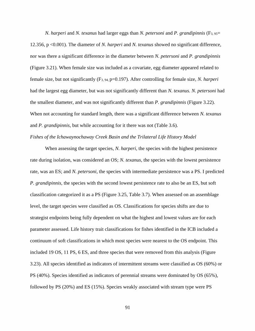
91
N. harperi and N. texanus had larger eggs than N. petersoni and P. grandipinnis (F3, 95=
12.356, p <0.001). The diameter of N. harperi and N. texanus showed no significant difference,
nor was there a significant difference in the diameter between N. petersoni and P. grandipinnis
(Figure 3.21). When female size was included as a covariate, egg diameter appeared related to
female size, but not significantly (F3, 94, p=0.197). After controlling for female size, N. harperi
had the largest egg diameter, but was not significantly different than N. texanus. N. petersoni had
the smallest diameter, and was not significantly different than P. grandipinnis (Figure 3.22).
When not accounting for standard length, there was a significant difference between N. texanus
and P. grandipinnis, but while accounting for it there was not (Table 3.6).
Fishes of the Ichawaynochaway Creek Basin and the Trilateral Life History Model
When assessing the target species, N. harperi, the species with the highest persistence
rate during isolation, was considered an OS; N. texanus, the species with the lowest persistence
rate, was an ES; and N. petersoni, the species with intermediate persistence was a PS. I predicted
P. grandipinnis, the species with the second lowest persistence rate to also be an ES, but soft
classification categorized it as a PS (Figure 3.25, Table 3.7). When assessed on an assemblage
level, the target species were classified as OS. Classifications for species shifts are due to
strategist endpoints being fully dependent on what the highest and lowest values are for each
parameter assessed. Life history trait classifications for fishes identified in the ICB included a
continuum of soft classifications in which most species were nearest to the OS endpoint. This
included 19 OS, 11 PS, 6 ES, and three species that were removed from this analysis (Figure
3.23). All species identified as indicators of intermittent streams were classified as OS (60%) or
PS (40%). Species identified as indicators of perennial streams were dominated by OS (65%),
followed by PS (20%) and ES (15%). Species weakly associated with stream type were PS
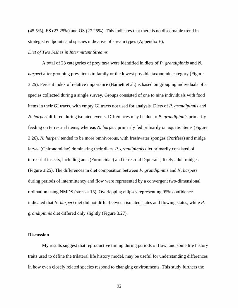
92
(45.5%), ES (27.25%) and OS (27.25%). This indicates that there is no discernable trend in
strategist endpoints and species indicative of stream types (Appendix E).
Diet of Two Fishes in Intermittent Streams
A total of 23 categories of prey taxa were identified in diets of P. grandipinnis and N.
harperi after grouping prey items to family or the lowest possible taxonomic category (Figure
3.25). Percent index of relative importance (Barnett et al.) is based on grouping individuals of a
species collected during a single survey. Groups consisted of one to nine individuals with food
items in their GI tracts, with empty GI tracts not used for analysis. Diets of P. grandipinnis and
N. harperi differed during isolated events. Differences may be due to P. grandipinnis primarily
feeding on terrestrial items, whereas N. harperi primarily fed primarily on aquatic items (Figure
3.26). N. harperi tended to be more omnivorous, with freshwater sponges (Porifera) and midge
larvae (Chironomidae) dominating their diets. P. grandipinnis diet primarily consisted of
terrestrial insects, including ants (Formicidae) and terrestrial Dipterans, likely adult midges
(Figure 3.25). The differences in diet composition between P. grandipinnis and N. harperi
during periods of intermittency and flow were represented by a convergent two-dimensional
ordination using NMDS (stress=.15). Overlapping ellipses representing 95% confidence
indicated that N. harperi diet did not differ between isolated states and flowing states, while P.
grandipinnis diet differed only slightly (Figure 3.27).
Discussion
My results suggest that reproductive timing during periods of flow, and some life history
traits used to define the trilateral life history model, may be useful for understanding differences
in how even closely related species respond to changing environments. This study furthers the
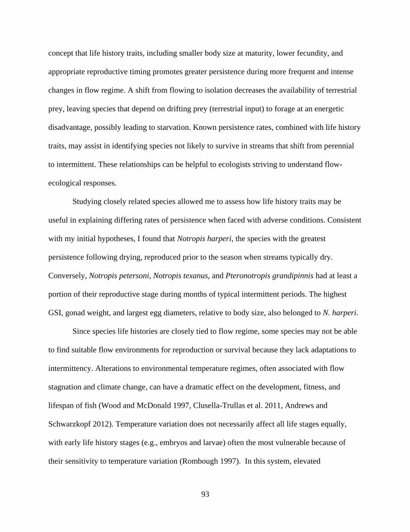
93
concept that life history traits, including smaller body size at maturity, lower fecundity, and
appropriate reproductive timing promotes greater persistence during more frequent and intense
changes in flow regime. A shift from flowing to isolation decreases the availability of terrestrial
prey, leaving species that depend on drifting prey (terrestrial input) to forage at an energetic
disadvantage, possibly leading to starvation. Known persistence rates, combined with life history
traits, may assist in identifying species not likely to survive in streams that shift from perennial
to intermittent. These relationships can be helpful to ecologists striving to understand flow-
ecological responses.
Studying closely related species allowed me to assess how life history traits may be
useful in explaining differing rates of persistence when faced with adverse conditions. Consistent
with my initial hypotheses, I found that Notropis harperi, the species with the greatest
persistence following drying, reproduced prior to the season when streams typically dry.
Conversely, Notropis petersoni, Notropis texanus, and Pteronotropis grandipinnis had at least a
portion of their reproductive stage during months of typical intermittent periods. The highest
GSI, gonad weight, and largest egg diameters, relative to body size, also belonged to N. harperi.
Since species life histories are closely tied to flow regime, some species may not be able
to find suitable flow environments for reproduction or survival because they lack adaptations to
intermittency. Alterations to environmental temperature regimes, often associated with flow
stagnation and climate change, can have a dramatic effect on the development, fitness, and
lifespan of fish (Wood and McDonald 1997, Clusella-Trullas et al. 2011, Andrews and
Schwarzkopf 2012). Temperature variation does not necessarily affect all life stages equally,
with early life history stages (e.g., embryos and larvae) often the most vulnerable because of
their sensitivity to temperature variation (Rombough 1997). In this system, elevated
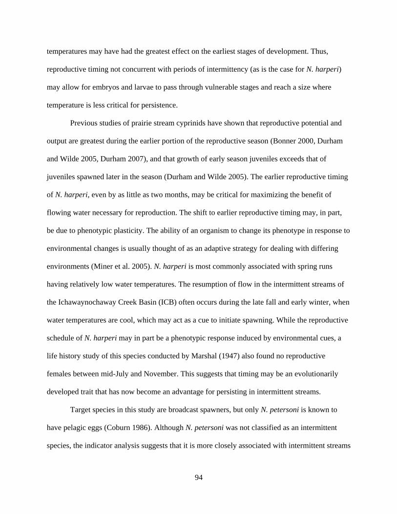
94
temperatures may have had the greatest effect on the earliest stages of development. Thus,
reproductive timing not concurrent with periods of intermittency (as is the case for N. harperi)
may allow for embryos and larvae to pass through vulnerable stages and reach a size where
temperature is less critical for persistence.
Previous studies of prairie stream cyprinids have shown that reproductive potential and
output are greatest during the earlier portion of the reproductive season (Bonner 2000, Durham
and Wilde 2005, Durham 2007), and that growth of early season juveniles exceeds that of
juveniles spawned later in the season (Durham and Wilde 2005). The earlier reproductive timing
of N. harperi, even by as little as two months, may be critical for maximizing the benefit of
flowing water necessary for reproduction. The shift to earlier reproductive timing may, in part,
be due to phenotypic plasticity. The ability of an organism to change its phenotype in response to
environmental changes is usually thought of as an adaptive strategy for dealing with differing
environments (Miner et al. 2005). N. harperi is most commonly associated with spring runs
having relatively low water temperatures. The resumption of flow in the intermittent streams of
the Ichawaynochaway Creek Basin (ICB) often occurs during the late fall and early winter, when
water temperatures are cool, which may act as a cue to initiate spawning. While the reproductive
schedule of N. harperi may in part be a phenotypic response induced by environmental cues, a
life history study of this species conducted by Marshal (1947) also found no reproductive
females between mid-July and November. This suggests that timing may be an evolutionarily
developed trait that has now become an advantage for persisting in intermittent streams.
Target species in this study are broadcast spawners, but only N. petersoni is known to
have pelagic eggs (Coburn 1986). Although N. petersoni was not classified as an intermittent
species, the indicator analysis suggests that it is more closely associated with intermittent streams
95
than perennial streams (p=0.07, Appendix E). Perkin and Gido (2010) identified human
fragmentation in streams as an overarching cause of declining prairie stream fishes that produce
semi-buoyant eggs. With increases in stream intermittency in the lower Flint River Basin over
the last few decades, N. petersoni might be expected to decline given the reductions of flow for
dispersal of developing embryos. Without flow and continued mixing of waters, developing
embryos may sink to the bottom of isolated pools, where they are subjected to siltation, high
concentration of ammonia, and low dissolved oxygen (DO) levels. While the other study species
have non-buoyant/adhesive eggs, reproducing during intermittent events may still be detrimental
to young fishes if eggs are spawned in areas that become dry.
Parental investment via GSI and gonad weight were much greater in N. harperi,
indicating a substantial investment per individual offspring compared to the other target species.
In an Oklahoma prairie stream, Spranza and Stanley (2000) found that fish occupying areas of
the stream with greater environmental fluctuations were not at an energetic or reproductive
disadvantage, and had equal or greater GSI scores compared to fish occupying more stable areas.
This may indicate that species persisting in variable areas can tolerate apparently adverse
conditions by maximizing other benefits (e.g., low predation or competition during isolation). N.
harperi exploit periods of intermittency to their advantage, allowing for this greater investment
in offspring.
Egg diameter tended to be greater for N. harperi, but not significantly so. It has been
demonstrated that egg diameter can be related to standard length among fishes at different sites
(Heins and Baker 1987, Casten and Johnston 2008), which is consistent with my results. I found
a difference in egg diameter between N. texanus and P. grandipinnis, but not after accounting for
standard length. This indicates that the egg diameter difference between the species could be

96
driven by female body size. In contrast, the significant difference in egg diameter between N.
harperi and P. grandipinnis, and the similarity between N. harperi and N. texanus, were
consistent and independent of female body size, suggesting differences among species will be
maintained within or among survey sites. Differences in egg diameter may be explained by
environmental variations affecting investment, whereby phenotypic variation and environmental
fluctuation may alter parental investment. Due to extirpation of species early on at intermittent
sites, this could not be examined more fully, therefore differences within and among these
species are still largely unknown.
Life-history theory predicts that the magnitude, frequency, and predictability of flow
regime events, including floods and droughts, can affect how organisms evolve (Iwasa and Levin
1995, Lytle and Poff 2004). When aquatic systems are altered from their natural flow regime, the
traits that allow species to persist over generations may become less suitable. It has been
demonstrated that flow alteration caused by dams can foster increases in non-native fishes
(Pringle et al. 2000). As flow becomes more stable, equilibrium strategists (ES) increase, while
periodic strategists (PS) and opportunistic strategists OS decrease (Mims and Olden 2013, Perkin
et al. 2017). Classification of strategy endpoints within the trilateral life history theory is
primarily dependent on what species are included in assessing distances to strategy endpoints.
On a basin scale, my results are similar to previous life history studies that follow Mims et al.
(2010) classification of species on the trilateral life history model, where fish assemblages in
intermittent stream classes tend to affiliate towards opportunistic endpoints (McManamay and
Frimpong 2015). However, species strongly associated with intermittent streams were classified
as both OS and PS. There were also no discernable differences among species commonly
associated with perennial streams, or weakly associated with either stream type. Within the

97
context of the species assemblage in the ICB (with rare species removed), all of the target
species were classified as OS. Based on persistence rates during isolated events (Figure 2.12,
Figure 2.13), we know that each of these species responds differently to intermittency.
When examining only target species against the trilateral history model, N. harperi was
classified as OS. This classification was driven primarily by its small length at maturation and
low fecundity. GSI and gonad weight is highest for N. harperi, indicating that although fecundity
was low, investment per egg was high. High investment per offspring, combined with
reproductive timing during periods when low-flows or intermittency do not occur, may be
indicative of why this species commonly occurs in intermittent streams rather than a small body
size at maturity and low fecundity. ES are predicted to be favored under stable conditions, and
this is consistent for N. texanus, the species with the lowest persistence rates. While predictions
coincided with persistence rates, spawning timing coinciding with intermittency may hinder N.
texanus from being successful in intermittent streams more so than a larger body size at maturity.
N. petersoni and P. grandipinnis are classified as PS, and are associated with predictable but
seasonally fluctuating environments. Consistent with findings that persistence is low during
isolation for these species, McManamay et al. (2015) found that PS species tended to decrease
with increasing intermittency; however, within their analysis all target species would have been
classified as OS rather than PS. It is because of this that life history models may be suited to
explaining general shifts in species trends, but may not be useful for exploring species-specific
changes to altered stream flow. Some aspects of the trilateral life history model, including length
at fecundity, as well as reproductive timing and diet can help explain why some species persist
better than others during intermittency.
98
Cyprinids are among the most abundant and diverse vertebrates in streams of the
southeastern US, and can therefore have potentially large effects on trophic dynamics and
ecological functions (Wheeler et al. 2017). Local extirpation of individuals in isolated pools did
not allow for assessing diet of all the target species. However, I did find a shift in feeding
patterns for P. grandipinnis, but not for N. harperi. For P. grandipinnis, this shift was primarily
driven by the lack of terrestrial diet items during isolated periods. Decreases in terrestrial
invertebrate input are known to lower fish biomass in headwater streams (Kawaguchi et al.
2003), as flow cessation lowers the availability of terrestrial prey items. While not evident in the
percent index of relative importance, guts of P. grandipinnis were frequently empty (personal
observation), which may suggest limited food availability. Contrary to hypotheses, shifts in diet
were not driven by a more advantageous opportunistic feeding pattern during isolation, but by
the lack of terrestrial prey items found. Given that the diet of N. harperi consists primarily of
aquatic items, the fact their feeding patterns did not shift likely means this species had an
energetic advantage for feeding during periods of isolation.
Life history traits of stream fishes partly reflect adaptations to natural flow regimes, and
trait-based approaches, including the trilateral life history model, have been useful for
understanding species responses to streamflow alteration. Native fishes in Coastal Plain stream
systems of southwestern GA, including the four study species, vary in occurrence and tolerance
to intermittency. I found that high persistence of one species corresponded to reproduction before
streams dry down, a small size at maturity, a greater reproductive investment, and a diet not
dependent on a terrestrial prey. All four species examined would be considered opportunistic
strategists within the trilateral life history model framework. However, my results suggest that
life history models, along with reproductive timing and diet, can help explain why even closely

99
related species differ in ability to persist in intermittent streams. The identification of species
differences in persistence probabilities in intermittent streams allows for the influence of life
history traits to be systematically explored. Understanding which life history traits are associated
with species persistence can help advance the understanding of flow ecology relationships.
100
References:
Albanese, B., J. T. Peterson, B. J. Freeman, and D. A. Weiler. 2007. Accounting for incomplete
detection when estimating site occupancy of Bluenose Shiner (Pteronotropis welaka) in
southwest Georgia. Southeastern Naturalist 6:657-668
Andrews, R. M., and L. Schwarzkopf. 2012. Thermal performance of squamate embryos with
respect to climate, adult life history, and phylogeny. Biological Journal of the Linnean
Society 106:851-864.
Barnett, T. P., D. W. Pierce, H. G. Hidalgo, C. Bonfils, B. D. Santer, T. Das, G. Bala, A. W.
Wood, T. Nozawa, and A. A. Mirin. 2008. Human-induced changes in the hydrology of
the western United States. Science 319:1080-1083.
Beitinger, T. L., W. A. Bennett, and R. W. McCauley. 2000. Temperature tolerances of North
American freshwater fishes exposed to dynamic changes in temperature. Environmental
Biology of Fishes 58:237-275.
Bennett, M. G., M. R. Whiles, and G. W. Whitledge. 2016. Population-level responses of life
history traits to flow regime in three common stream fish species. Ecohydrology 9:1388-
1399.
Bonner, T. H. 2000. Life history and reproductive ecology of the Arkansas River shiner and
peppered chub in the Canadian River, Texas and New Mexico. Texas Tech University,
Doctoral dissertatin.
Brown, T. C., R. Foti, and J. A. Ramirez. 2013. Projected freshwater withdrawals in the United
States under a changing climate. Water Resources Research 49:1259-1276.
Bunn, S. E., and A. H. Arthington. 2002. Basic principles and ecological consequences of altered
flow regimes for aquatic biodiversity. Environmental Management 30:492-507.
Carlisle, D. M., D. M. Wolock, and M. R. Meador. 2011. Alteration of streamflow magnitudes
and potential ecological consequences: a multiregional assessment. Frontiers in Ecology
and the Environment 9:264-270.
Casten, L. R., and C. E. Johnston. 2008. Life-history plasticity among stream sites in the
Chattahoochee River drainage, Alabama. Southeastern Naturalist 7:679-690.
Clarke, K. R. 1993. Non-parametric multivariate analyses of changes in community structure.
Australian Journal of Ecology 18:117-143.
Clusella-Trullas, S., T. M. Blackburn, and S. L. Chown. 2011. Climatic predictors of temperature
performance curve parameters in ectotherms imply complex responses to climate change.
The American Naturalist 177:738-751.
101
Coburn, M. M. 1986. Egg diameter variation in eastern North American minnows (Pisces:
Cyprinidae): correlation with vertebral number, habitat and spawning behavior. Ohio
Journal of Science 86(3):110-120.
De Cáceres, M. 2010. Indicspecies R package (ver. 1.4.0). Online [URL] http://sites. google.
com/site/miqueldecaceres/software.
Durham, B. W. 2007. Reproductive ecology, habitat associations, and population dynamics of
two imperiled cyprinids in a Great Plains river. Texas Tech University, Doctoral
dissertation.
Durham, B. W., and G. R. Wilde. 2005. Relationship between hatch date and first-summer
growth of five species of prairie-stream cyprinids. Environmental Biology of Fishes
72:45-54.
Echelle, A. A., A. F. Echelle, and L. G. Hill. 1972. Interspecific interactions and limiting factors
of abundance and distribution in the Red River pupfish, Cyprinodon rubrofluviatilis.
American Midland Naturalist 1:109-130.
Falke, J. A., K. D. Fausch, R. Magelky, A. Aldred, D. S. Durnford, L. K. Riley, and R. Oad.
2011. The role of groundwater pumping and drought in shaping ecological futures for
stream fishes in a dryland river basin of the western Great Plains, USA. Ecohydrology
4:682-697.
Fausch, K. D., and R. G. Bramblett. 1991. Disturbance and fish communities in intermittent
tributaries of a western Great Plains river. Copeia 1991:659-674.
Fox, J., S. Weisberg, D. Adler, D. Bates, G. Baud-Bovy, S. Ellison, D. Firth, M. Friendly, G.
Gorjanc, and S. Graves. 2017. Package ‘car’. Version.
Frimpong, E. A., and P. L. Angermeier. 2010. Trait-based approaches in the analysis of stream
fish communities. American Fisheries Society, Symposium. Community ecology of
stream fishes: concepts, approaches, and techniques:109-136.
Golladay, S. W., and J. Battle. 2001. Does the Chickasawhatchee swamp influence water quality.
Proceedings of the 2001 Georgia Water Resources Conference. Institute of Ecology, The
University of Georgia. Athens, Georgia.
Golladay, S. W., and D. W. Hicks. 2013. Indicators of long term hydrologic change in the Flint
River. Proceedings of the 2013 Georgia Water Resources Conference. Institute of
Ecology, The University of Georgia. Athens, Georgia.
Grover, J. J. 1998. Feeding habits of pelagic summer flounder, Paralichthys dentatus, larvae in
oceanic and estuarine habitats. Fishery Bulletin 96:248-257.
102
Heins, D. C., and J. A. Baker. 1987. Analysis of factors associated with intraspecific variation in
propagule size of a stream-dwelling fish. Community and evolutionary ecology of North
American stream fishes. University of Oklahoma Press, Norman:223-231.
Heins, D. C., and J. A. Baker. 1993. Clutch Production in the Darter Etheostoma lynceum and its
Implications for Life-History Study. Journal of Fish Biology 42:819-829.
Heins, D. C., and J. A. Baker. 1999. Evaluation of ovum storage techniques for reproductive
studies of fishes. Ecology of Freshwater Fish 8(2):65-69.
Heins, D. C., and F. G. Rabito. 1986. Spawning performance in North American minnows: direct
evidence of the occurrence of multiple clutches in the genus Notropis. Journal of Fish
Biology 28:343.
Hicks, D. W., H. E. Gill, and S. A. Longsworth. 1987. Hydrogeology, chemical quality, and
availability of groundwater in the upper Floridan Aquifer, Albany Area, Georgia. USGS
Water-Resources Investigations Report 87.
Hughey, M. C., D. C. Heins, H. L. Jelks, B. A. Ory, and F. Jordan. 2012. Variation in
Reproductive Life History Traits between Two Populations of Blackbanded Darters
(Percina nigrofasciata). Copeia 2012:714-721.
Iwasa, Y., and S. A. Levin. 1995. The timing of life history events. Journal of Theoretical
Biology 172:33.
Kawaguchi, Y., Y. Taniguchi, and S. Nakano. 2003. Terrestrial invertebrate inputs determine the
local abundance of stream fishes in a forested stream. Ecology 84:701-708.
Kennard, M. J., S. J. Mackay, B. J. Pusey, J. D. Olden, and N. Marsh. 2010. Quantifying
uncertainty in estimation of hydrologic metrics for ecohydrological studies. River
Research and Applications 26:137-156.
Lake, P. S. 2003. Ecological effects of perturbation by drought in flowing waters. Freshwater
Biology 48:1161-1172.
Lamouroux, N., N. L. Poff, and P. L. Angermeier. 2002. Intercontinental convergence of stream
fish community traits along geomorphic and hydraulic gradients. Ecology 83:1792-1807.
Larned, S. T., T. Datry, D. B. Arscott, and K. Tockner. 2010. Emerging concepts in temporary-
river ecology. Freshwater Biology 55:717-738.
Lenth, R. V. 2016. Least-squares means: the R package lsmeans. J Stat Software 69:1-33.
Logez, M., D. Pont, and M. T. Ferreira. 2010. Do Iberian and European fish faunas exhibit
convergent functional structure along environmental gradients? Journal of the North
American Benthological Society 29:1310-1323.
103
Lytle, D. A., and N. L. Poff. 2004. Adaptation to natural flow regimes. Trends in Ecology &
Evolution 19:94-100.
Marshall, N. 1947. The spring run and cave habitats of Erimystax harperi (Fowler). Ecology
28:68-75.
Matthews, W. J., and E. Marsh-Matthews. 2003. Effects of drought on fish across axes of space,
time and ecological complexity. Freshwater Biology 48:1232-1253.
McManamay, R. A., M. S. Bevelhimer, and E. A. Frimpong. 2015. Associations among
hydrologic classifications and fish traits to support environmental flow standards.
Ecohydrology 8:460-479.
McManamay, R. A., and E. A. Frimpong. 2015. Hydrologic filtering of fish life history strategies
across the United States: implications for stream flow alteration. Ecological Applications
25:243-263.
Mims, M. C., and J. D. Olden. 2013. Fish assemblages respond to altered flow regimes via
ecological filtering of life history strategies. Freshwater Biology 58:50-62.
Mims, M. C., J. D. Olden, Z. R. Shattuck, and N. L. Poff. 2010. Life history trait diversity of
native freshwater fishes in North America. Ecology of Freshwater Fish 19:390-400.
Miner, B. G., S. E. Sultan, S. G. Morgan, D. K. Padilla, and R. A. Relyea. 2005. Ecological
consequences of phenotypic plasticity. Trends in Ecology & Evolution 20:685-692.
Naiman, R. J., J. J. Latterell, N. E. Pettit, and J. D. Olden. 2008. Flow variability and the
biophysical vitality of river systems. Comptes Rendus Geoscience 340:629-643.
Oksanen, J., F. G. Blanchet, R. Kindt, P. Legendre, P. R. Minchin, R. O’hara, G. L. Simpson, P.
Solymos, M. H. H. Stevens, and H. Wagner. 2013. Package ‘vegan’. Community ecology
package, version 2.
Opsahl, S. P., S. E. Chapal, D. W. Hicks, and C. K. Wheeler. 2007. Evaluation of ground-water
and surface-water exchanges using streamflow difference analyses. Journal of the
American Water Resources Association 43:1132-1141.
Palmer, M. A., C. A. Reidy Liermann, C. Nilsson, M. Flörke, J. Alcamo, P. S. Lake, and N.
Bond. 2008. Climate change and the world's river basins: anticipating management
options. Frontiers in Ecology and the Environment 6:81-89.
Perkin, J. S., K. B. Gido, E. Johnson, and V. M. Tabor. 2010. Consequences of stream
fragmentation and climate change for rare Great Plains fishes. Final Report to USFWS
Great Plains Landscape Conservation Cooperative Program.
104
Perkin, J. S., N. E. Knorp, T. C. Boersig, A. E. Gebhard, L. A. Hix, and T. C. Johnson. 2017.
Life history theory predicts long-term fish assemblage response to stream impoundment.
Canadian Journal of Fisheries & Aquatic Sciences 74:228-239.
Pinheiro, J., D. Bates, S. DebRoy, and D. Sarkar. 2014. nlme: linear and nonlinear mixed effects
models. R package version 3.1-117. Available at h ttp://CRAN. R-project. org/package=
nlme.
Pinkas, L., M. S. Oliphant, and I. L. K. Iverson. 1971. Food habits of albacore, bluefin tuna, and
bonito in California waters. California, Department of Fish and Game. Fish Bulletin
152:1-105.
Poff, L. N. 1997. Landscape filters and species traits: towards mechanistic understanding and
prediction in stream ecology. Journal of the North American Benthological Society
16(2):391-409.
Poff, N. L., and J. D. Allan. 1995. Functional-organization of stream fish assemblages in relation
to hydrological variability. Ecology 76:606-627.
Poff, N. L., J. D. Olden, N. K. Vieira, D. S. Finn, M. P. Simmons, and B. C. Kondratieff. 2006.
Functional trait niches of North American lotic insects: traits-based ecological
applications in light of phylogenetic relationships. Journal of the North American
Benthological Society 25:730-755.
Power, M. E., A. Sun, G. Parker, W. E. Dietrich, and J. T. Wootton. 1995. Hydraulic food-chain
models. Bioscience 45(3):159-167.
Pringle, C. M., M. C. Freeman, and B. J. Freeman. 2000. Regional effects of hydrologic
alterations on riverine macrobiota in the New World: tropical-temperate comparisons.
Bioscience 50:807-823.
R Core Team. 2014. R: A language and environment for statistical computing. Vienna, Austria:
R Foundation for Statistical Computing. Available: http://cran.rproject.org (June 2017).
Resh, V. H., A. V. Brown, A. P. Covich, M. E. Gurtz, H. W. Li, G. W. Minshall, S. R. Reice, A.
L. Sheldon, J. B. Wallace, and R. C. Wissmar. 1988. The role of disturbance in stream
ecology. Journal of the North American Benthological Society 7:433-455.
Rombough, P. J. 1997. The effects of temperature on embryonic and larval development.
Seminar Series-Society For Experimental Biology. Cambridge University Press 66:177-
224.
Smith, C. C., and S. D. Fretwell. 1974. The optimal balance between size and number of
offspring. The American Naturalist 108(962):499-506.
105
Spranza, J. J., and E. H. Stanley. 2000. Condition, growth, and reproductive styles of fishes
exposed to different environmental regimes in a prairie drainage. Environmental Biology
of Fishes 59:99-109.
Stearns, S. C. 1977. The evolution of life history traits: a critique of the theory and a review of
the data. Annual Review of Ecology and Systematics 8(1):145-171.
Taylor, C. M. 1997. Fish species richness and incidence patterns in isolated and connected
stream pools: effects of pool volume and spatial position. Oecologia 110:560-566.
Tedesco, P. A., B. Hugueny, T. Oberdorff, H. H. Dürr, S. Mérigoux, B. De Mérona, and R.
Brandl. 2008. River hydrological seasonality influences life history strategies of tropical
riverine fishes. Oecologia 156:691-702.
Torak, L. J., and J. A. Painter. 2006. Geohydrology of the lower Apalachicola-Chattahoochee-
Flint River basin, southwestern Georgia, northwestern Florida, and southeastern
Alabama. U.S. Geological Survey, Report Number 2006-5070. Atlanta, GA.
Townsend, C. R., and A. G. Hildrew. 1994. Species traits in relation to a habitat templet for river
systems. Freshwater Biology 31:265-275.
Van Der Kraak, G., and N. W. Pankhurst. 1997. Temperature effects on the reproductive
performance of fish. Seminar Series. Society for Experimental Biology 61:159-176.
Wheeler, K., S. J. Wenger, and M. C. Freeman. 2017. States and rates: Complementary
approaches to developing flow-ecology relationships. Freshwater Biology: 2017 in press.
Winemiller, K. O. 1989. Patterns of Variation in Life History among South American Fishes in
Seasonal Environments. Oecologia 81(2):225-241.
Winemiller, K. O. 2005. Life history strategies, population regulation, and implications for
fisheries management. Canadian Journal of Fisheries and Aquatic Sciences 62:872-885.
Winemiller, K. O., and K. A. Rose. 1992. Patterns of life-history diversification in North
American fishes: implications for population regulation. Canadian Journal of Fisheries
and Aquatic Sciences 49:2196-2218.
Wood, C. M., and D. G. McDonald. 1997. Global warming: implications for freshwater and
marine fish. Cambridge University Press, No. 61.
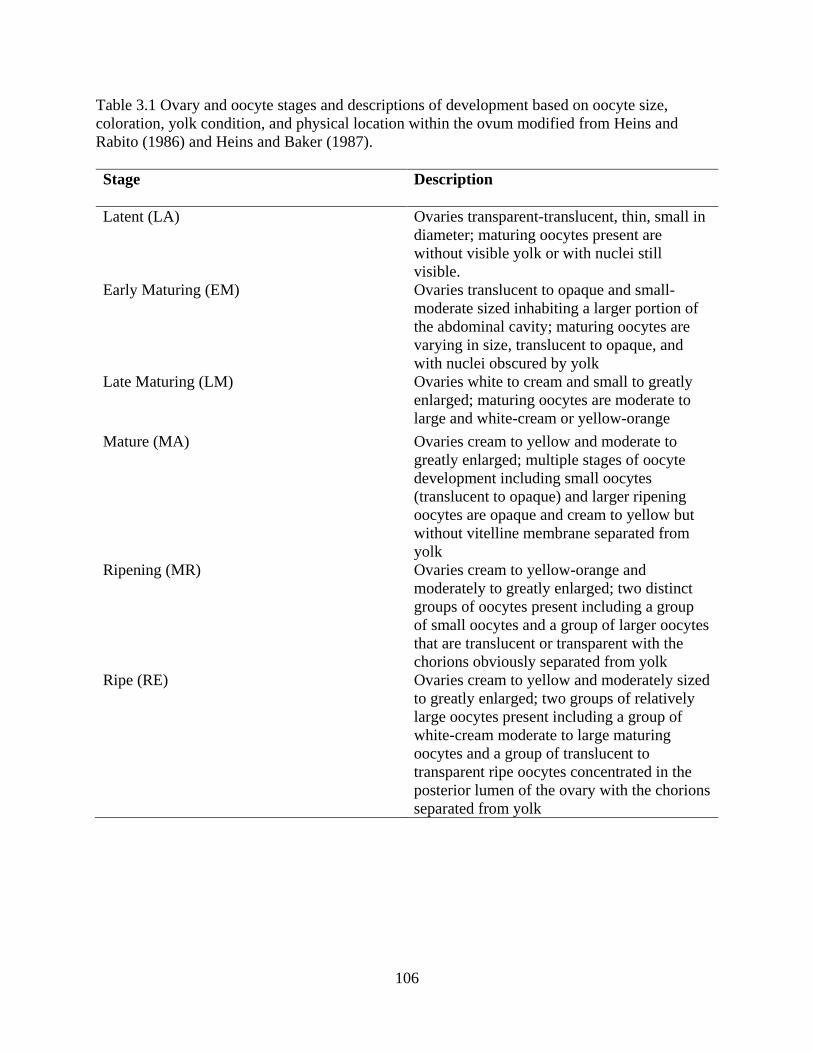
106
Table 3.1 Ovary and oocyte stages and descriptions of development based on oocyte size,
coloration, yolk condition, and physical location within the ovum modified from Heins and
Rabito (1986) and Heins and Baker (1987).
Stage Description
Latent (LA) Ovaries transparent-translucent, thin, small in
diameter; maturing oocytes present are
without visible yolk or with nuclei still
visible.
Early Maturing (EM) Ovaries translucent to opaque and small-
moderate sized inhabiting a larger portion of
the abdominal cavity; maturing oocytes are
varying in size, translucent to opaque, and
with nuclei obscured by yolk
Late Maturing (LM) Ovaries white to cream and small to greatly
enlarged; maturing oocytes are moderate to
large and white-cream or yellow-orange
Mature (MA) Ovaries cream to yellow and moderate to
greatly enlarged; multiple stages of oocyte
development including small oocytes
(translucent to opaque) and larger ripening
oocytes are opaque and cream to yellow but
without vitelline membrane separated from
yolk
Ripening (MR) Ovaries cream to yellow-orange and
moderately to greatly enlarged; two distinct
groups of oocytes present including a group
of small oocytes and a group of larger oocytes
that are translucent or transparent with the
chorions obviously separated from yolk
Ripe (RE) Ovaries cream to yellow and moderately sized
to greatly enlarged; two groups of relatively
large oocytes present including a group of
white-cream moderate to large maturing
oocytes and a group of translucent to
transparent ripe oocytes concentrated in the
posterior lumen of the ovary with the chorions
separated from yolk
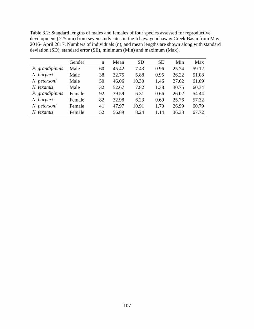
107
Table 3.2: Standard lengths of males and females of four species assessed for reproductive
development (>25mm) from seven study sites in the Ichawaynochaway Creek Basin from May
2016- April 2017. Numbers of individuals (n), and mean lengths are shown along with standard
deviation (SD), standard error (SE), minimum (Min) and maximum (Max).
Gender n Mean SD SE Min Max
P. grandipinnis Male 60 45.42 7.43 0.96 25.74 59.12
N. harperi Male 38 32.75 5.88 0.95 26.22 51.08
N. petersoni Male 50 46.06 10.30 1.46 27.62 61.09
N. texanus Male 32 52.67 7.82 1.38 30.75 60.34
P. grandipinnis Female 92 39.59 6.31 0.66 26.02 54.44
N. harperi Female 82 32.98 6.23 0.69 25.76 57.32
N. petersoni Female 41 47.97 10.91 1.70 26.99 60.79
N. texanus Female 52 56.89 8.24 1.14 36.33 67.72
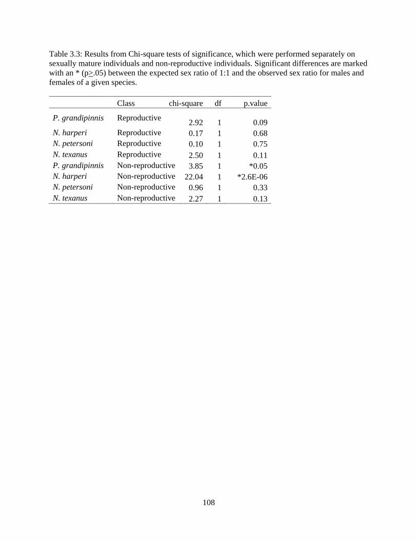
108
Table 3.3: Results from Chi-square tests of significance, which were performed separately on
sexually mature individuals and non-reproductive individuals. Significant differences are marked
with an * (p>.05) between the expected sex ratio of 1:1 and the observed sex ratio for males and
females of a given species.
Class chi-square df p.value
P. grandipinnis Reproductive 2.92 1 0.09
N. harperi Reproductive 0.17 1 0.68
N. petersoni Reproductive 0.10 1 0.75
N. texanus Reproductive 2.50 1 0.11
P. grandipinnis Non-reproductive 3.85 1 *0.05
N. harperi Non-reproductive 22.04 1 *2.6E-06
N. petersoni Non-reproductive 0.96 1 0.33
N. texanus Non-reproductive 2.27 1 0.13
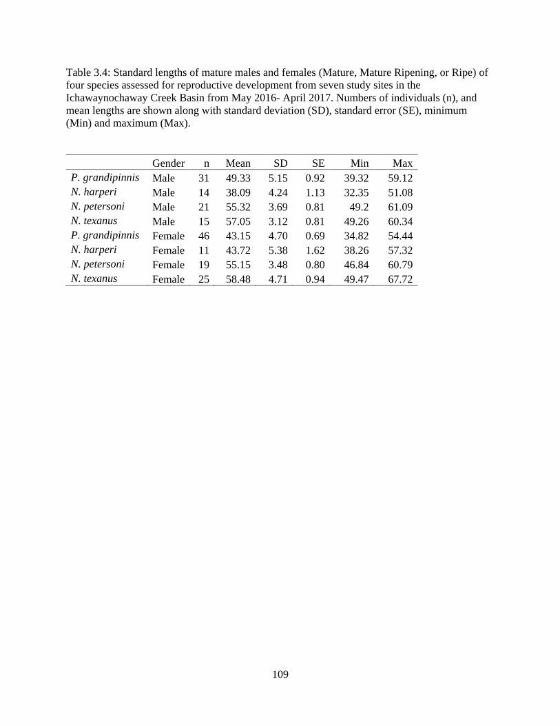
109
Table 3.4: Standard lengths of mature males and females (Mature, Mature Ripening, or Ripe) of
four species assessed for reproductive development from seven study sites in the
Ichawaynochaway Creek Basin from May 2016- April 2017. Numbers of individuals (n), and
mean lengths are shown along with standard deviation (SD), standard error (SE), minimum
(Min) and maximum (Max).
Gender n Mean SD SE Min Max
P. grandipinnis Male 31 49.33 5.15 0.92 39.32 59.12
N. harperi Male 14 38.09 4.24 1.13 32.35 51.08
N. petersoni Male 21 55.32 3.69 0.81 49.2 61.09
N. texanus Male 15 57.05 3.12 0.81 49.26 60.34
P. grandipinnis Female 46 43.15 4.70 0.69 34.82 54.44
N. harperi Female 11 43.72 5.38 1.62 38.26 57.32
N. petersoni Female 19 55.15 3.48 0.80 46.84 60.79
N. texanus Female 25 58.48 4.71 0.94 49.47 67.72
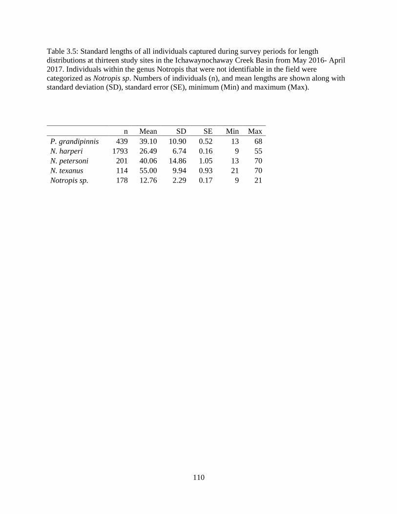
110
Table 3.5: Standard lengths of all individuals captured during survey periods for length
distributions at thirteen study sites in the Ichawaynochaway Creek Basin from May 2016- April
2017. Individuals within the genus Notropis that were not identifiable in the field were
categorized as Notropis sp. Numbers of individuals (n), and mean lengths are shown along with
standard deviation (SD), standard error (SE), minimum (Min) and maximum (Max).
n Mean SD SE Min Max
P. grandipinnis 439 39.10 10.90 0.52 13 68
N. harperi 1793 26.49 6.74 0.16 9 55
N. petersoni 201 40.06 14.86 1.05 13 70
N. texanus 114 55.00 9.94 0.93 21 70
Notropis sp. 178 12.76 2.29 0.17 9 21

111
Table 3.6: Summary statistics for egg size (mm) of mature, mature ripening, and ripe females
assessed for reproductive investment. Each individual had twenty eggs measured, where n is the
number of individuals assessed per species. Numbers of individuals (n), and mean lengths are
shown along with standard deviation (SD), standard error (SE), minimum (Min) and maximum
(Max).
n Mean SD SE Min Max
P. grandipinnis 47 0.87 0.08 0.004 0.65 1.2
N. harperi 9 0.99 0.16 0.017 0.75 1.45
N. petersoni 18 0.88 0.10 0.008 0.65 1.15
N. texanus 25 0.98 0.12 0.007 0.75 1.3
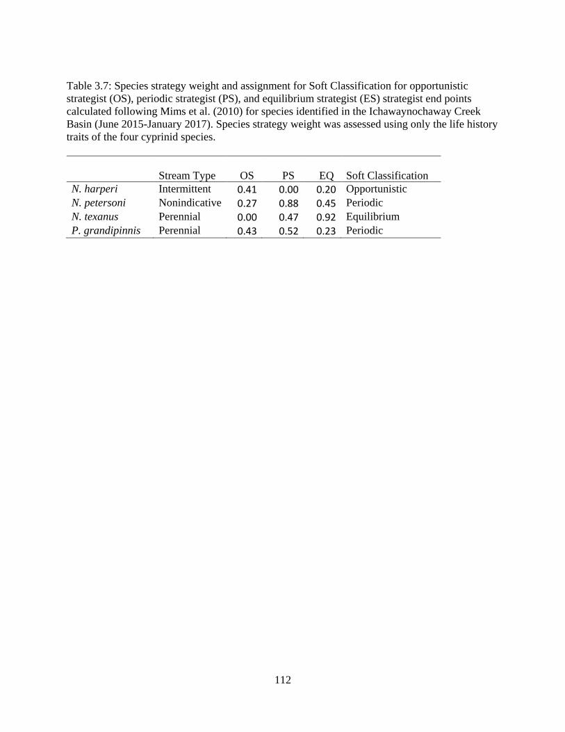
112
Table 3.7: Species strategy weight and assignment for Soft Classification for opportunistic
strategist (OS), periodic strategist (PS), and equilibrium strategist (ES) strategist end points
calculated following Mims et al. (2010) for species identified in the Ichawaynochaway Creek
Basin (June 2015-January 2017). Species strategy weight was assessed using only the life history
traits of the four cyprinid species.
Stream Type OS PS EQ Soft Classification
N. harperi Intermittent 0.41 0.00 0.20 Opportunistic
N. petersoni Nonindicative 0.27 0.88 0.45 Periodic
N. texanus Perennial 0.00 0.47 0.92 Equilibrium
P. grandipinnis Perennial 0.43 0.52 0.23 Periodic
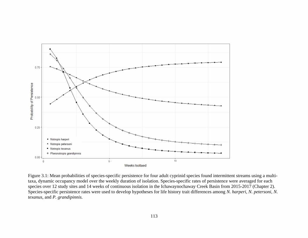
113
Figure 3.1: Mean probabilities of species-specific persistence for four adult cyprinid species found intermittent streams using a multi-
taxa, dynamic occupancy model over the weekly duration of isolation. Species-specific rates of persistence were averaged for each
species over 12 study sites and 14 weeks of continuous isolation in the Ichawaynochaway Creek Basin from 2015-2017 (Chapter 2).
Species-specific persistence rates were used to develop hypotheses for life history trait differences among N. harperi, N. petersoni, N.
texanus, and P. grandipinnis.

114
Figure 3.2: Locations of thirteen study sites within the Ichawaynochaway Creek Basin that were used to measure length distributions
for four cyprinid species and to obtain individuals for analyzing diet and reproductive characteristics, May 2016- April 2017. Apart
from Brantley Creek (the most north easterly circle) all survey streams are intermittent and experienced isolation or complete drying
during the survey period.

115
Figure 3.3: Standard length distribution to the nearest millimeter for all P. grandipinnis individuals found at thirteen study sites within
the Ichawaynochaway Creek Basin from May 2016- April 2017, plotted by Julian date. The horizontal line represents the minimum
reported length at maturity (34.82 mm standard length).
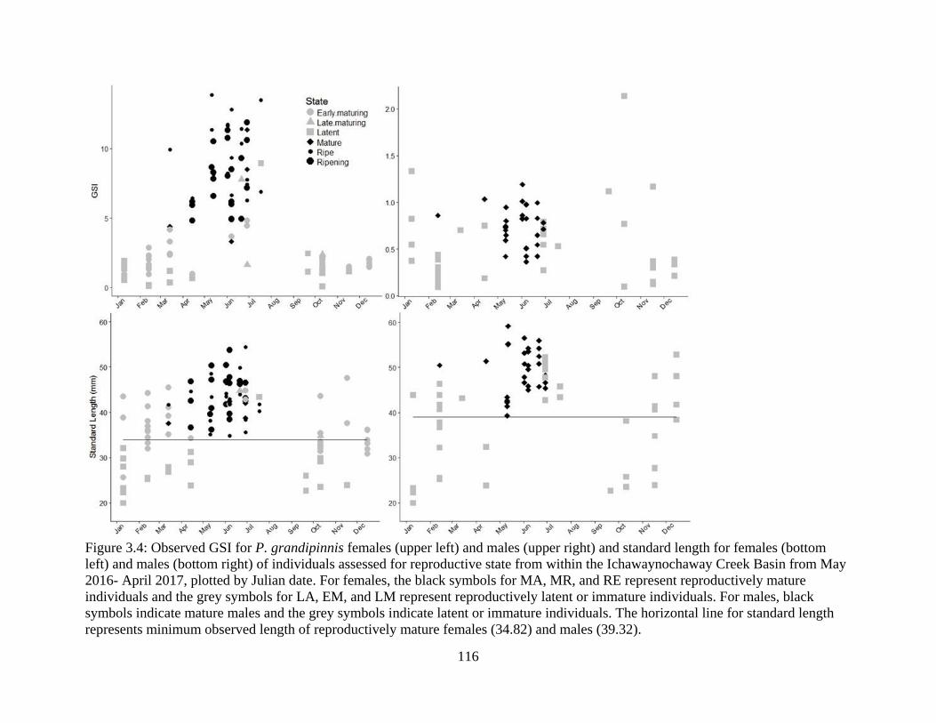
116
Figure 3.4: Observed GSI for P. grandipinnis females (upper left) and males (upper right) and standard length for females (bottom
left) and males (bottom right) of individuals assessed for reproductive state from within the Ichawaynochaway Creek Basin from May
2016- April 2017, plotted by Julian date. For females, the black symbols for MA, MR, and RE represent reproductively mature
individuals and the grey symbols for LA, EM, and LM represent reproductively latent or immature individuals. For males, black
symbols indicate mature males and the grey symbols indicate latent or immature individuals. The horizontal line for standard length
represents minimum observed length of reproductively mature females (34.82) and males (39.32).
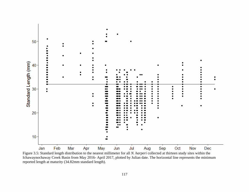
117
Figure 3.5: Standard length distribution to the nearest millimeter for all N. harperi collected at thirteen study sites within the
Ichawaynochaway Creek Basin from May 2016- April 2017, plotted by Julian date. The horizontal line represents the minimum
reported length at maturity (34.82mm standard length).
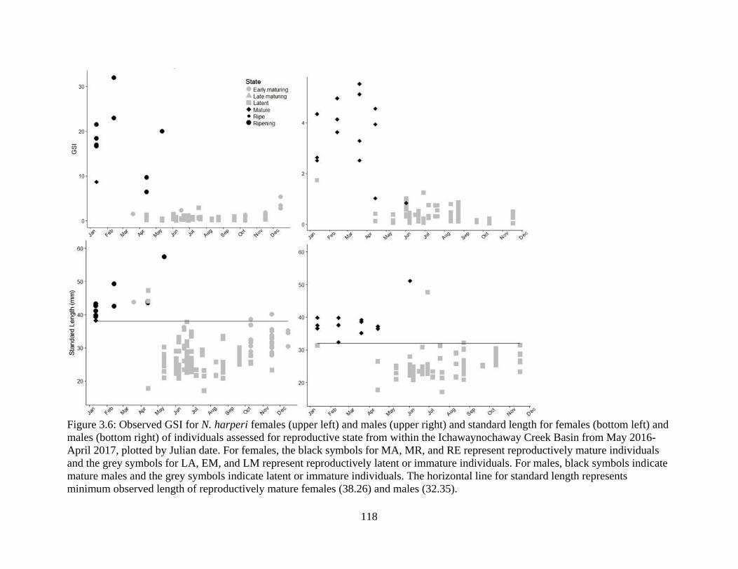
118
Figure 3.6: Observed GSI for N. harperi females (upper left) and males (upper right) and standard length for females (bottom left) and
males (bottom right) of individuals assessed for reproductive state from within the Ichawaynochaway Creek Basin from May 2016-
April 2017, plotted by Julian date. For females, the black symbols for MA, MR, and RE represent reproductively mature individuals
and the grey symbols for LA, EM, and LM represent reproductively latent or immature individuals. For males, black symbols indicate
mature males and the grey symbols indicate latent or immature individuals. The horizontal line for standard length represents
minimum observed length of reproductively mature females (38.26) and males (32.35).
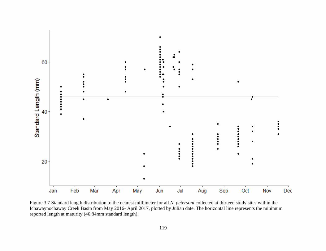
119
Figure 3.7 Standard length distribution to the nearest millimeter for all N. petersoni collected at thirteen study sites within the
Ichawaynochaway Creek Basin from May 2016- April 2017, plotted by Julian date. The horizontal line represents the minimum
reported length at maturity (46.84mm standard length).
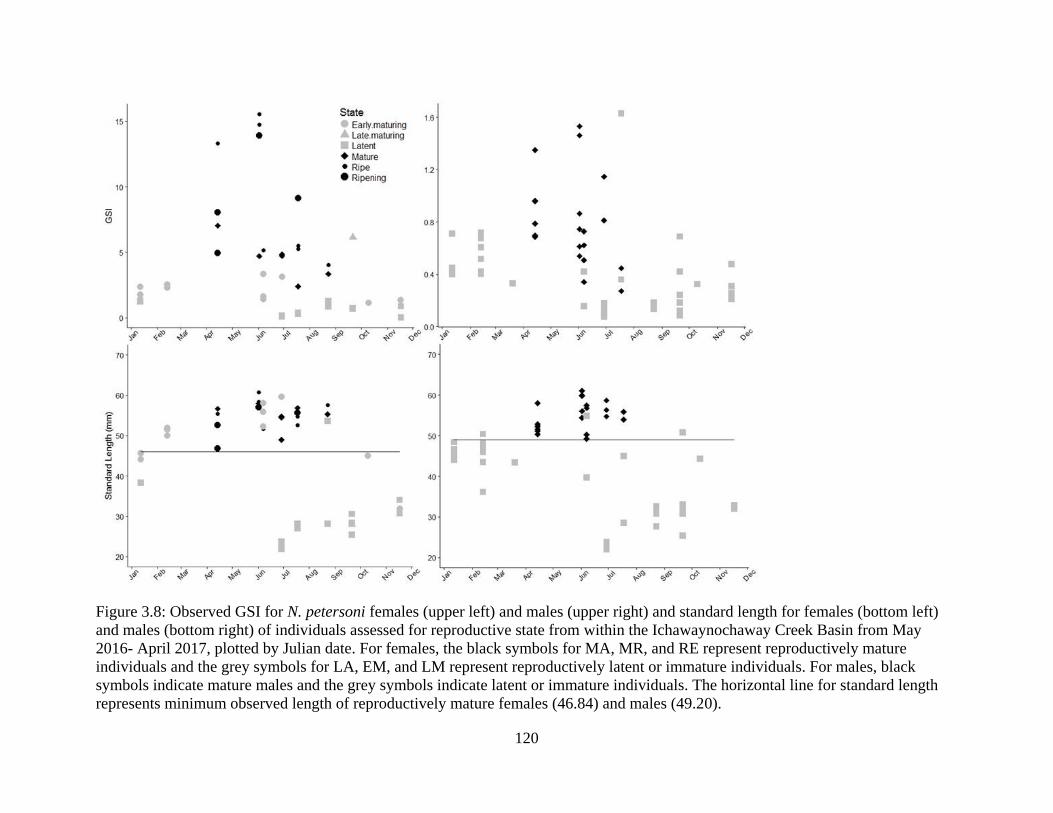
120
Figure 3.8: Observed GSI for N. petersoni females (upper left) and males (upper right) and standard length for females (bottom left)
and males (bottom right) of individuals assessed for reproductive state from within the Ichawaynochaway Creek Basin from May
2016- April 2017, plotted by Julian date. For females, the black symbols for MA, MR, and RE represent reproductively mature
individuals and the grey symbols for LA, EM, and LM represent reproductively latent or immature individuals. For males, black
symbols indicate mature males and the grey symbols indicate latent or immature individuals. The horizontal line for standard length
represents minimum observed length of reproductively mature females (46.84) and males (49.20).
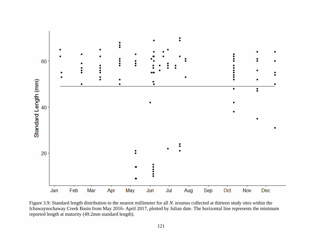
121
Figure 3.9: Standard length distribution to the nearest millimeter for all N. texanus collected at thirteen study sites within the
Ichawaynochaway Creek Basin from May 2016- April 2017, plotted by Julian date. The horizontal line represents the minimum
reported length at maturity (49.2mm standard length).
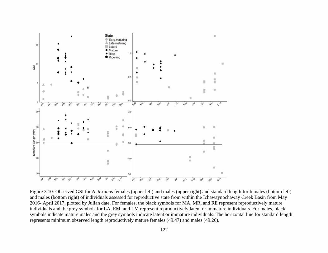
122
Figure 3.10: Observed GSI for N. texanus females (upper left) and males (upper right) and standard length for females (bottom left)
and males (bottom right) of individuals assessed for reproductive state from within the Ichawaynochaway Creek Basin from May
2016- April 2017, plotted by Julian date. For females, the black symbols for MA, MR, and RE represent reproductively mature
individuals and the grey symbols for LA, EM, and LM represent reproductively latent or immature individuals. For males, black
symbols indicate mature males and the grey symbols indicate latent or immature individuals. The horizontal line for standard length
represents minimum observed length reproductively mature females (49.47) and males (49.26).
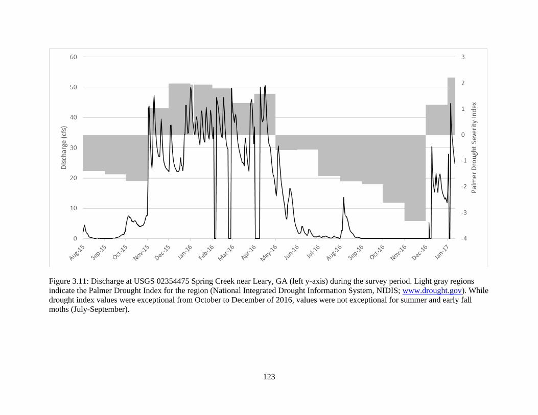
123
Figure 3.11: Discharge at USGS 02354475 Spring Creek near Leary, GA (left y-axis) during the survey period. Light gray regions
indicate the Palmer Drought Index for the region (National Integrated Drought Information System, NIDIS; www.drought.gov). While
drought index values were exceptional from October to December of 2016, values were not exceptional for summer and early fall
moths (July-September).
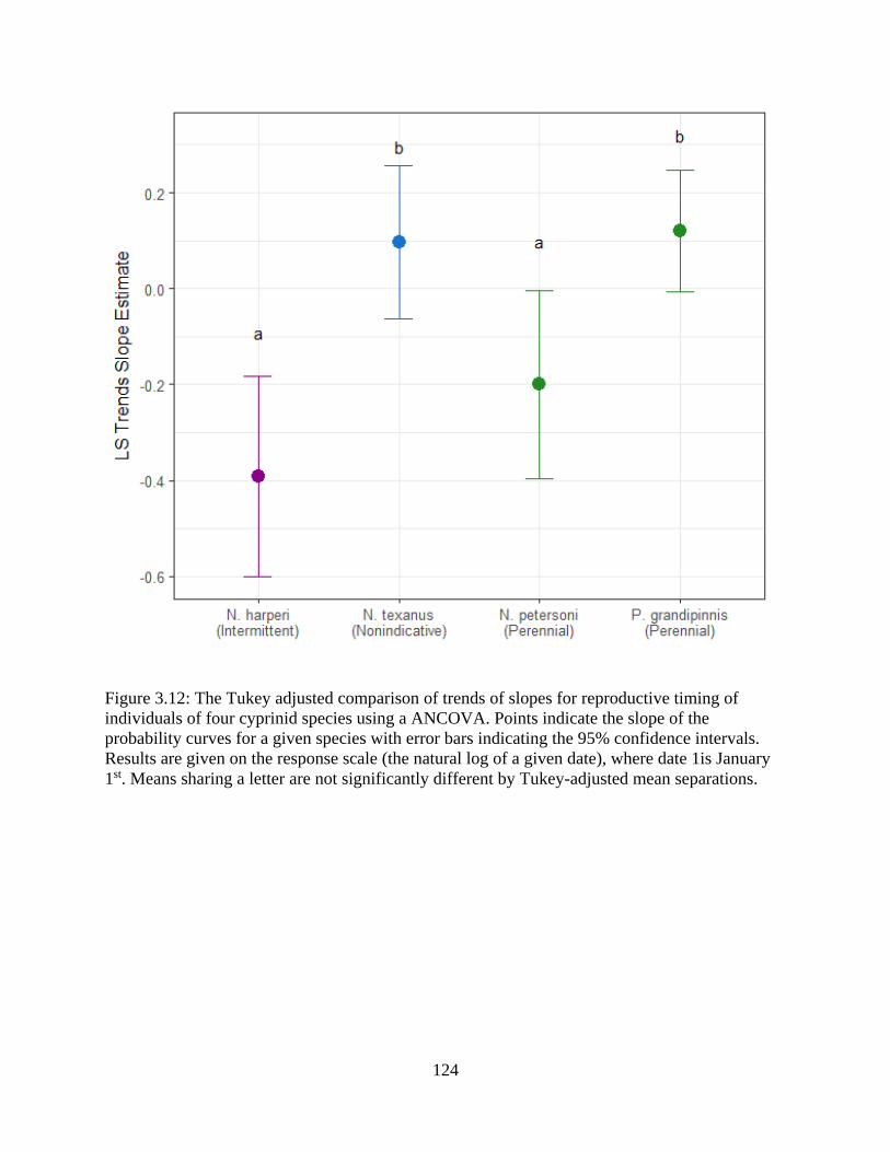
124
Figure 3.12: The Tukey adjusted comparison of trends of slopes for reproductive timing of
individuals of four cyprinid species using a ANCOVA. Points indicate the slope of the
probability curves for a given species with error bars indicating the 95% confidence intervals.
Results are given on the response scale (the natural log of a given date), where date 1is January
1st. Means sharing a letter are not significantly different by Tukey-adjusted mean separations.
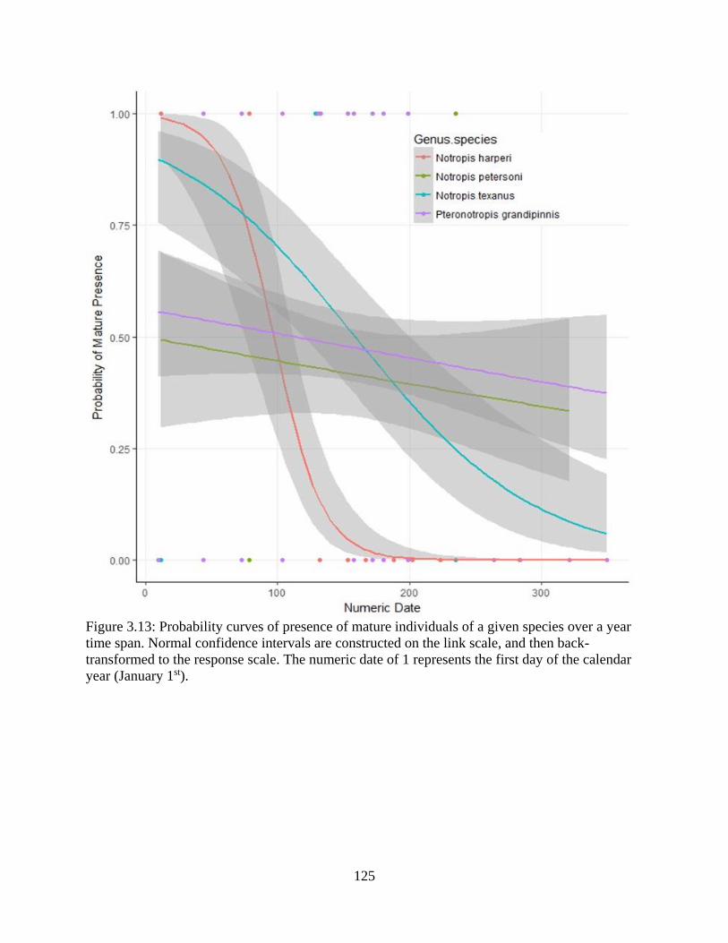
125
Figure 3.13: Probability curves of presence of mature individuals of a given species over a year
time span. Normal confidence intervals are constructed on the link scale, and then back-
transformed to the response scale. The numeric date of 1 represents the first day of the calendar
year (January 1st).
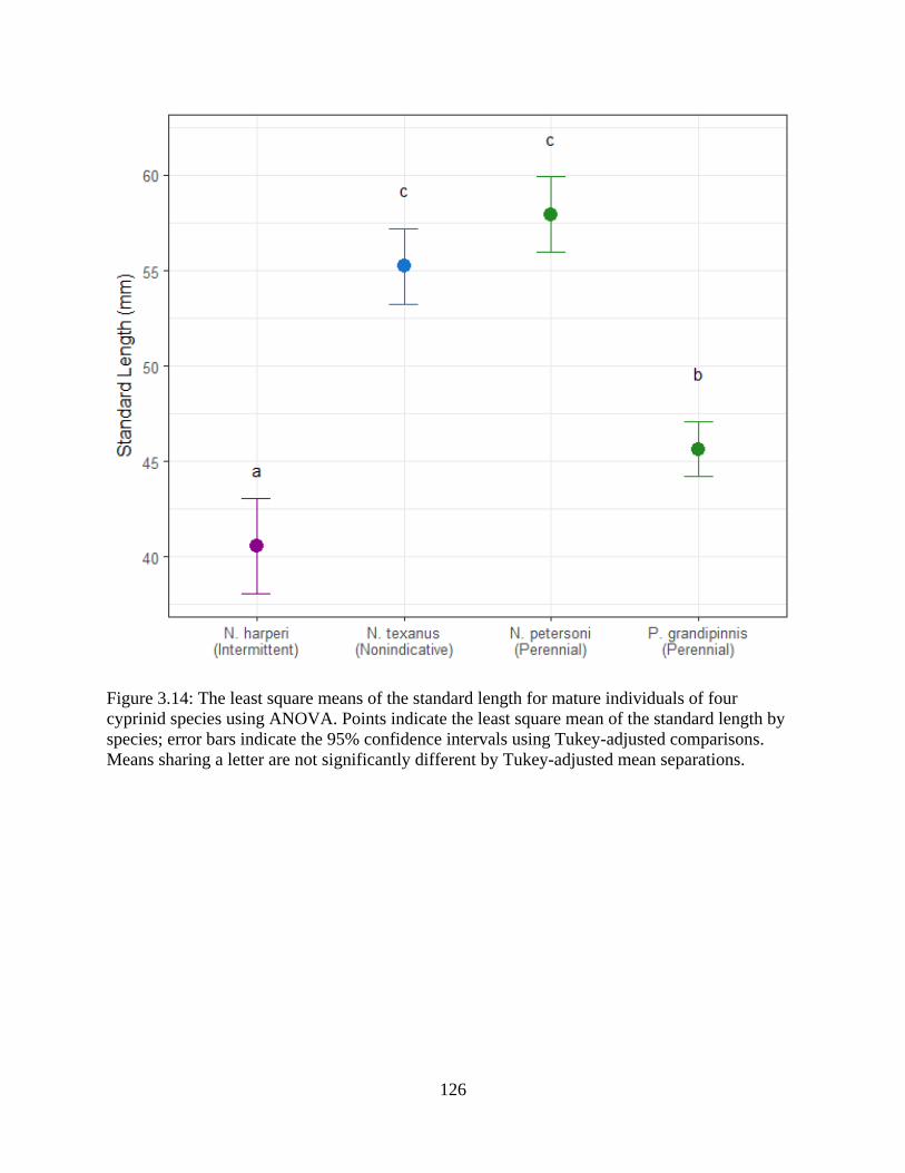
126
Figure 3.14: The least square means of the standard length for mature individuals of four
cyprinid species using ANOVA. Points indicate the least square mean of the standard length by
species; error bars indicate the 95% confidence intervals using Tukey-adjusted comparisons.
Means sharing a letter are not significantly different by Tukey-adjusted mean separations.
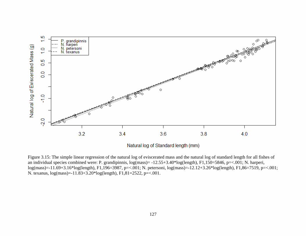
127
Figure 3.15: The simple linear regression of the natural log of eviscerated mass and the natural log of standard length for all fishes of
an individual species combined were: P. grandipinnis, log(mass)= -12.55+3.40*log(length), F1,150=5846, p=<.001; N. harperi,
log(mass)=-11.69+3.16*log(length), F1,196=3987, p=<.001; N. petersoni, log(mass)=-12.12+3.26*log(length), F1,86=7519, p=<.001;
N. texanus, log(mass)=-11.83+3.20*log(length), F1,81=2522, p=<.001.

128
Figure 3.16: The least square means of the eviscerated mass for mature males of four
cyprinid species using ANCOVA. Points indicate the least square mean of the eviscerated
mass of an individual and error bars indicate the 95% confidence intervals using Tukey-
adjusted comparisons. Means sharing a letter are not significantly different by Tukey-
adjusted mean separations.
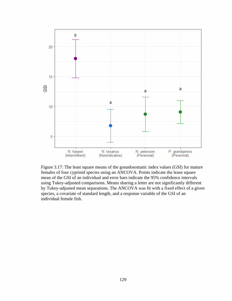
129
Figure 3.17: The least square means of the gonadosomatic index values (GSI) for mature
females of four cyprinid species using an ANCOVA. Points indicate the lease square
mean of the GSI of an individual and error bars indicate the 95% confidence intervals
using Tukey-adjusted comparisons. Means sharing a letter are not significantly different
by Tukey-adjusted mean separations. The ANCOVA was fit with a fixed effect of a given
species, a covariate of standard length, and a response variable of the GSI of an
individual female fish.
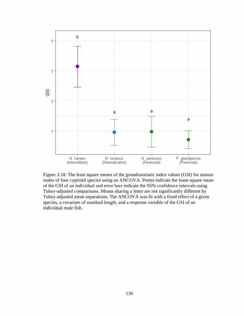
130
Figure 3.18: The least square means of the gonadosomatic index values (GSI) for mature
males of four cyprinid species using an ANCOVA. Points indicate the lease square mean
of the GSI of an individual and error bars indicate the 95% confidence intervals using
Tukey-adjusted comparisons. Means sharing a letter are not significantly different by
Tukey-adjusted mean separations. The ANCOVA was fit with a fixed effect of a given
species, a covariate of standard length, and a response variable of the GSI of an
individual male fish.
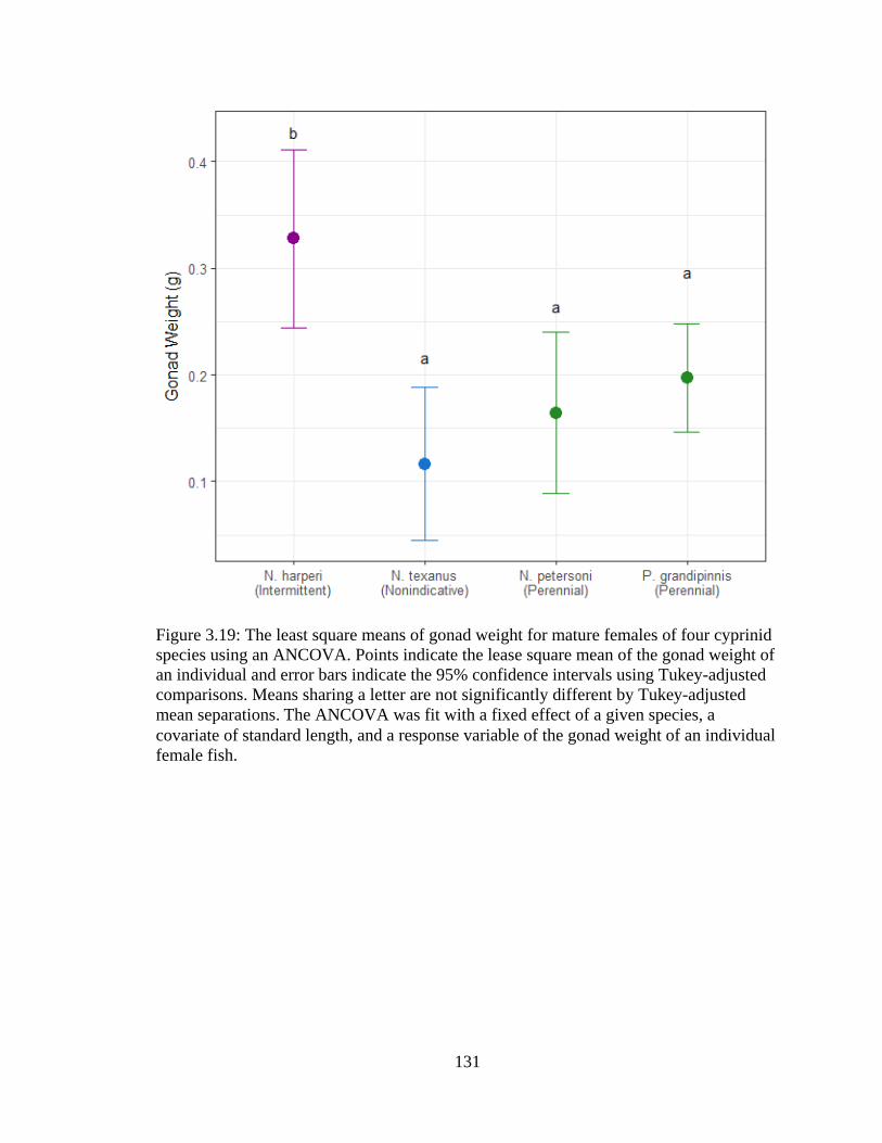
131
Figure 3.19: The least square means of gonad weight for mature females of four cyprinid
species using an ANCOVA. Points indicate the lease square mean of the gonad weight of
an individual and error bars indicate the 95% confidence intervals using Tukey-adjusted
comparisons. Means sharing a letter are not significantly different by Tukey-adjusted
mean separations. The ANCOVA was fit with a fixed effect of a given species, a
covariate of standard length, and a response variable of the gonad weight of an individual
female fish.
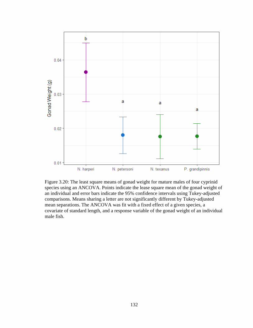
132
Figure 3.20: The least square means of gonad weight for mature males of four cyprinid
species using an ANCOVA. Points indicate the lease square mean of the gonad weight of
an individual and error bars indicate the 95% confidence intervals using Tukey-adjusted
comparisons. Means sharing a letter are not significantly different by Tukey-adjusted
mean separations. The ANCOVA was fit with a fixed effect of a given species, a
covariate of standard length, and a response variable of the gonad weight of an individual
male fish.
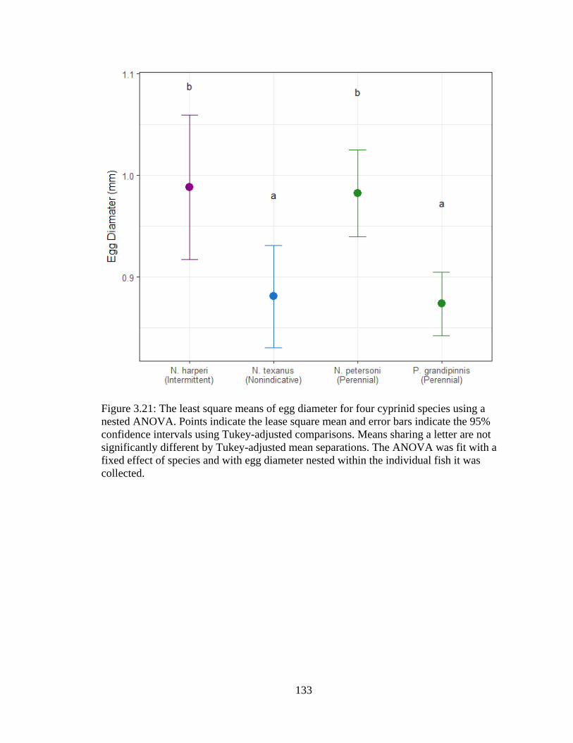
133
Figure 3.21: The least square means of egg diameter for four cyprinid species using a
nested ANOVA. Points indicate the lease square mean and error bars indicate the 95%
confidence intervals using Tukey-adjusted comparisons. Means sharing a letter are not
significantly different by Tukey-adjusted mean separations. The ANOVA was fit with a
fixed effect of species and with egg diameter nested within the individual fish it was
collected.
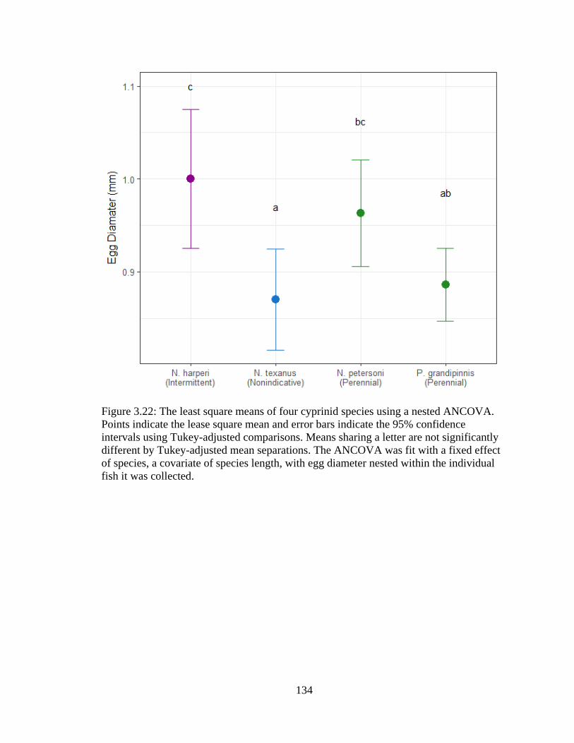
134
Figure 3.22: The least square means of four cyprinid species using a nested ANCOVA.
Points indicate the lease square mean and error bars indicate the 95% confidence
intervals using Tukey-adjusted comparisons. Means sharing a letter are not significantly
different by Tukey-adjusted mean separations. The ANCOVA was fit with a fixed effect
of species, a covariate of species length, with egg diameter nested within the individual
fish it was collected.

135
Figure 3.23: Ternary plot illustrating trilateral life history trade-offs in traits among commonly occurring species within the
Ichawaynochaway Creek basin. Axis scores indicate degree of species affiliation with opportunistic, periodic, or equilibrium
strategists. Species points are represented by which stream type they are associated with. The target species (P. grandipinnis, N.
harperi, N. petersoni, and N. texanus), represented by cross symbols, score highest on the opportunistic axis when evaluated in the
context of this assemblage.

136
Figure 3.24: Ternary plot illustrating trilateral life history trade-offs in traits among four cyprinid species, where axis scores indicate
degree of species affiliation with opportunistic, periodic, or equilibrium strategists.
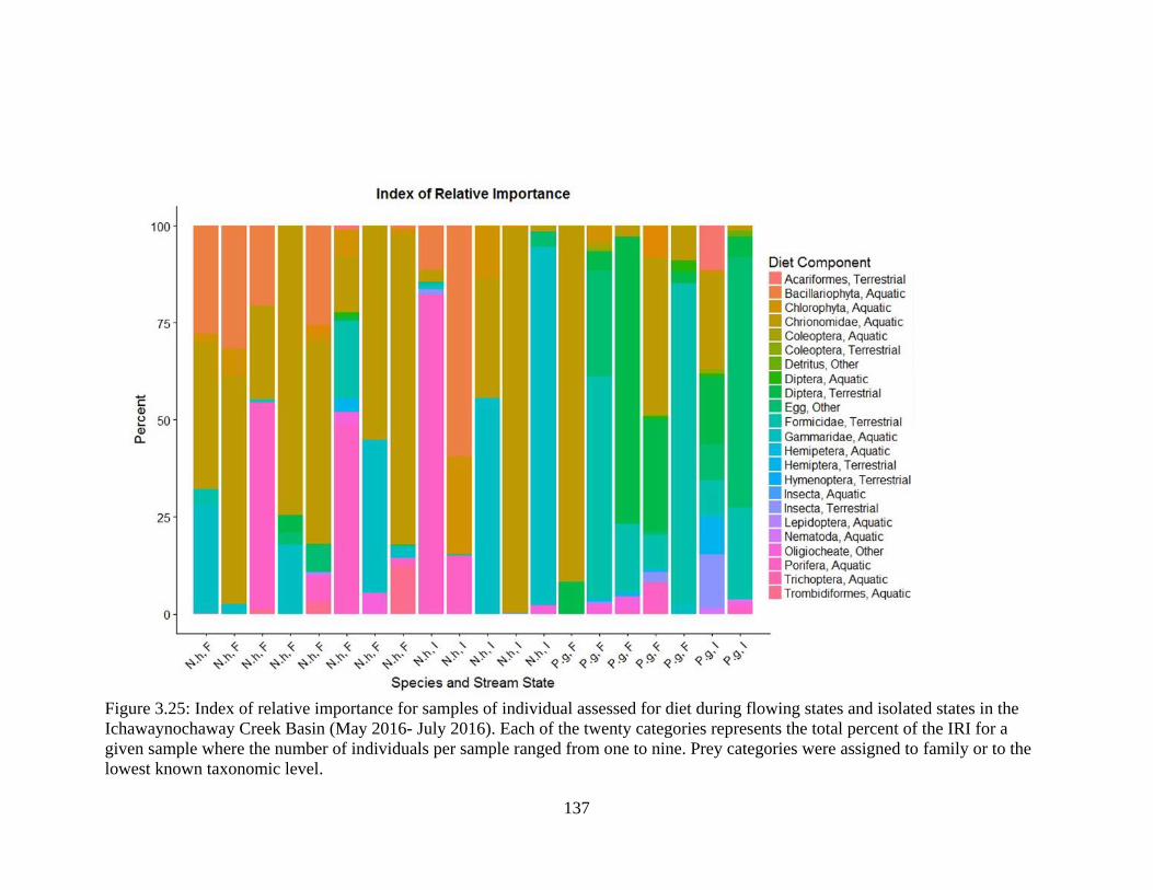
137
Figure 3.25: Index of relative importance for samples of individual assessed for diet during flowing states and isolated states in the
Ichawaynochaway Creek Basin (May 2016- July 2016). Each of the twenty categories represents the total percent of the IRI for a
given sample where the number of individuals per sample ranged from one to nine. Prey categories were assigned to family or to the
lowest known taxonomic level.
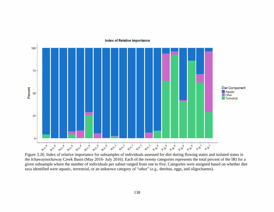
138
Figure 3.26: Index of relative importance for subsamples of individuals assessed for diet during flowing states and isolated states in
the Ichawaynochaway Creek Basin (May 2016- July 2016). Each of the twenty categories represents the total percent of the IRI for a
given subsample where the number of individuals per subset ranged from one to five. Categories were assigned based on whether diet
taxa identified were aquatic, terrestrial, or an unknown category of “other” (e.g., detritus, eggs, and oligochaetes).
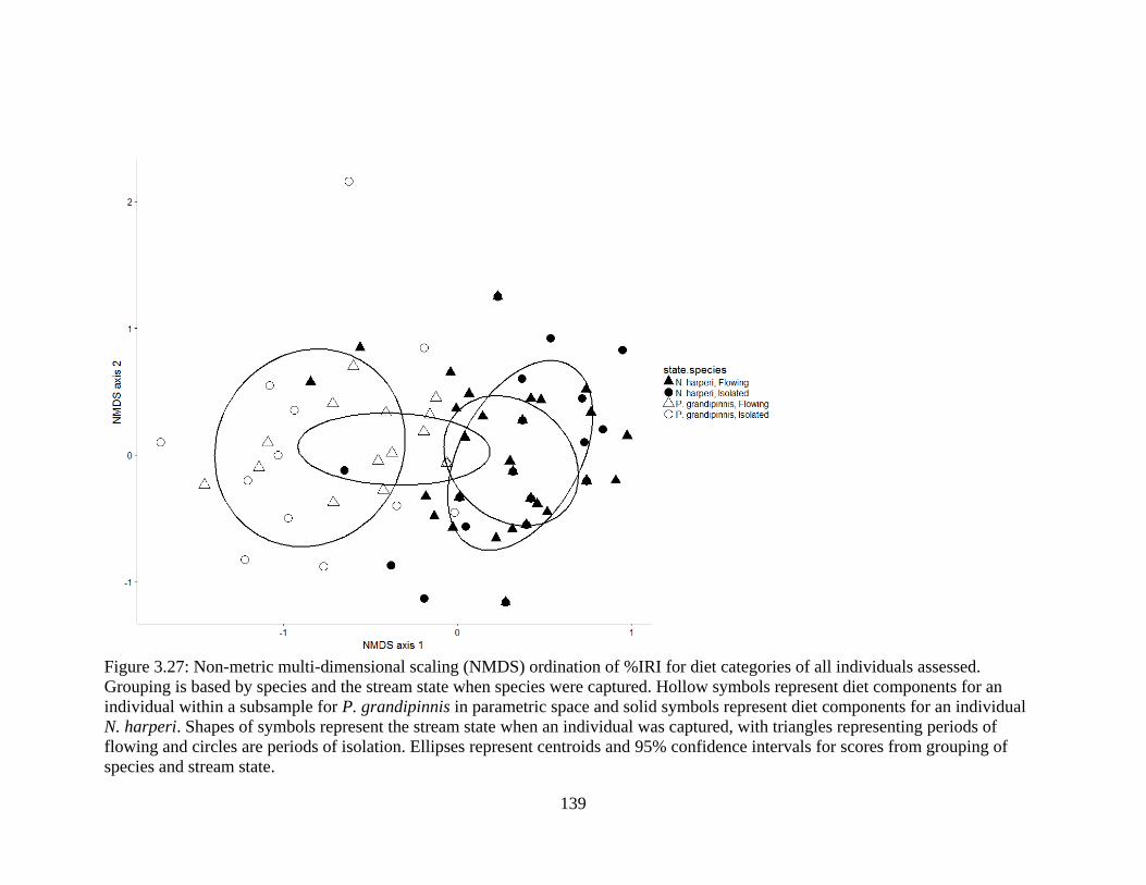
139
Figure 3.27: Non-metric multi-dimensional scaling (NMDS) ordination of %IRI for diet categories of all individuals assessed.
Grouping is based by species and the stream state when species were captured. Hollow symbols represent diet components for an
individual within a subsample for P. grandipinnis in parametric space and solid symbols represent diet components for an individual
N. harperi. Shapes of symbols represent the stream state when an individual was captured, with triangles representing periods of
flowing and circles are periods of isolation. Ellipses represent centroids and 95% confidence intervals for scores from grouping of
species and stream state.
140
CHAPTER 4
CONCLUSIONS AND SUMMARY
The development of the Ecological Limits of Hydrologic Alteration (ELOHA)
framework (Poff et al. 2010), along with placement of streams into hydrological classes,
provides a context for generalizing hydrologic disturbances, assembling and testing hypotheses
regarding ecological responses to hydrological disturbances, and developing environmental flow
standards (McManamay et al. 2015). By comparing ecological patterns between natural and
hydrologically altered streams, ecologists can develop flow-ecological response relationships
that can guide the creation of environmental flow standards (Arthington et al. 2006), whereby the
quantity, timing, and quality of water flows required to sustain freshwater ecosystems and human
livelihood are achieved (Poff et al. 2010). Understanding the biotic consequences of human
streamflow alteration is critical for successful environmental flow management.
Increased withdrawals from surface and groundwaters, coupled with climate change,
have altered stream hydrology in southwestern Georgia (Golladay et al. 2016). Recent multi-year
droughts have highlighted the need to apply flow-ecology relationships within the lower Flint
River basin, as the combined interaction of droughts and groundwater withdrawals have resulted
in many previously perennial streams ceasing to flow (Rugel et al. 2012). In particular, streams
crossing the Dougherty Plain, a recharge area for the upper Floridan aquifer region in the
southern portion of the lower Flint River basin, are prone to drying during periods of low rainfall
and high groundwater withdrawal (Opsahl et al. 2007). To understand the impacts of stream
drying and intermittency on biota within a tributary watershed of the lower Flint River,

141
Ichawaynochaway Creek, I examined fish assemblage variation across a gradient of flow
permanence, isolation, and reach position to quantify species-specific responses to changes in
abiotic conditions. I also explored life history traits to identify those most closely correlated with
species persistence in four cyprinids.
Fish community structure differs between intermittent and perennial streams, with the
former having a subset of species also occurring in perennial streams. I estimated rates of
species-specific occurrence, persistence, and colonization within streams that periodically ceased
flowing, and then determined the probability of occurrence in relation to environmental
characteristics. Indicator species of intermittent streams, as well as species that most commonly
occur, have the highest persistence rates as stream drying proceeds. Species that occurred in
isolated pools experienced greater rates of mortality as dissolved oxygen levels decreased and
ammonia concentrations increased. However, the ultimate driver of local extirpation was isolated
pools drying down to levels that exacerbated these effects. Like other studies of intermittent
streams, common species possessed both higher colonization and lower extinction rates than
rarer species (Whitney et al. 2016). Colonization of reaches after the resumption of flow
indicated that communities were able to recover, although ongoing intermittency decreased the
likelihood of recovery. This suggests that with the increasing frequency of low-flows and
intermittency within the ICB, indicator species of intermittent streams will become more
common, while indicator species of perennial streams will likely decline.
Four commonly occurring cyprinid species differed in rates of persistence in intermittent
streams during periods of isolation. For Notropis haperi, a species with high persistence rates,
reproductive timing did not overlap with typical seasonal stream drying, while species with low
persistence rates in isolated pools (Notropis petersoni, Notropis texanus, and Pteronotropis
142
grandipinnis) had at least a portion of their reproductive timing overlap with times when streams
were likely to dry. I demonstrated that some of the life history traits used to define the trilateral
life history model proposed by Kirk O. Winemiller (1989), including smaller body size at
maturity and low fecundity, may be useful for understanding how species respond to changing
environments. Studies have largely supported fish life history trait ordination along the three
axes of the trilateral life history model across North America (Kennard et al. 2010, Mims et al.
2010, Mims and Olden 2013, Perkin et al. 2017) as a means for predicting responses to natural
and altered flow regimes on fish assemblages through flow stabilization. Incorporating broadly
established models, feeding habits, and reproductive timing, may help in understanding
differences in how even closely related species respond to changing environments, while also
highlighting those traits most likely to promote greater persistence given more frequent and
intense disturbances.
Recent studies have indicated a need to quantify biotic response to changing flow
conditions through quantitative modeling (Arthington et al. 2006, Poff et al. 2010). Within the
lower Flint, water use during low-flow periods will result in both increased periods of flow
cessation in previously perennial streams, and increased dry periods in intermittent streams. The
southeastern US is noted for its aquatic faunal diversity, having the most diverse freshwater fish
fauna in North America (Burr and Mayden 1993). Reduction of diversity within streams due to
shifts in flow regime over time may result in the loss of sensitive species and an increase species
with high persistence.
143
References:
Arthington, A. H., S. E. Bunn, N. L. Poff, and R. J. Naiman. 2006. The challenge of providing
environmental flow rules to sustain river ecosystems. Ecological Applications 16:1311-
1318.
Burr, B. M., and R. L. Mayden. 1993. Phylogenetics and North American freshwater fishes.
Stanford University Press, Stanford, California.
Golladay, S. W., K. L. Martin, J. M. Vose, D. N. Wear, A. P. Covich, R. J. Hobbs, K. D.
Klepzig, G. E. Likens, R. J. Naiman, and A. W. Shearer. 2016. Review and synthesis:
achievable future conditions as a framework for guiding forest conservation and
management. Forest Ecology and Management 360:80-96.
Growns, I. 2004. A numerical classification of reproductive guilds of the freshwater fishes of
southeastern Australia and their application to river management. Fisheries management
and Ecology 11:369-377.
Kennard, M. J., S. J. Mackay, B. J. Pusey, J. D. Olden, and N. Marsh. 2010. Quantifying
uncertainty in estimation of hydrologic metrics for ecohydrological studies. River
Research and Applications 26:137-156.
McManamay, R. A., M. S. Bevelhimer, and E. A. Frimpong. 2015. Associations among
hydrologic classifications and fish traits to support environmental flow standards.
Ecohydrology 8:460-479.
Mims, M. C., and J. D. Olden. 2013. Fish assemblages respond to altered flow regimes via
ecological filtering of life history strategies. Freshwater Biology 58:50-62.
Mims, M. C., J. D. Olden, Z. R. Shattuck, and N. L. Poff. 2010. Life history trait diversity of
native freshwater fishes in North America. Ecology of Freshwater Fish 19:390-400.
Opsahl, S. P., S. E. Chapal, D. W. Hicks, and C. K. Wheeler. 2007. Evaluation of ground-water
and surface-water exchanges using streamflow difference analyses. Journal of the
American Water Resources Association 43:1132-1141.
Perkin, J. S., N. E. Knorp, T. C. Boersig, A. E. Gebhard, L. A. Hix, and T. C. Johnson. 2017.
Life history theory predicts long-term fish assemblage response to stream impoundment.
Canadian Journal of Fisheries & Aquatic Sciences 74:228-239.
Poff, N. L., B. D. Richter, A. H. Arthington, S. E. Bunn, R. J. Naiman, E. Kendy, M. Acreman,
C. Apse, B. P. Bledsoe, M. C. Freeman, J. Henriksen, R. B. Jacobson, J. G. Kennen, D.
M. Merritt, J. H. O'Keeffe, J. D. Olden, K. Rogers, R. E. Tharme, and A. Warner. 2010.
The ecological limits of hydrologic alteration (ELOHA): a new framework for
developing regional environmental flow standards. Freshwater Biology 55:147-170.
144
Rugel, K., C. R. Jackson, J. J. Romeis, S. W. Golladay, D. W. Hicks, and J. F. Dowd. 2012.
Effects of irrigation withdrawals on streamflows in a karst environment: lower Flint
River basin, Georgia, USA. Hydrological Processes 26:523-534.
Vila-Gispert, A., R. Moreno-Amich, and E. García-Berthou. 2002. Gradients of life-history
variation: an intercontinental comparison of fishes. Reviews in Fish Biology & Fisheries
12:417.
Wheeler, K., S. J. Wenger, and M. C. Freeman. 2017. States and rates: Complementary
approaches to developing flow-ecology relationships. Freshwater Biology. 2017 in press.
Whitney, J. E., K. B. Gido, E. C. Martin, and K. J. Hase. 2016. The first to arrive and the last to
leave: colonisation and extinction dynamics of common and rare fishes in intermittent
prairie streams. Freshwater Biology 61:1321-1334.
Winemiller, K. O. 1989. Patterns of Variation in Life History among South American Fishes in
Seasonal Environments. Oecologia 81(2):225-241.

145
APPENDICES
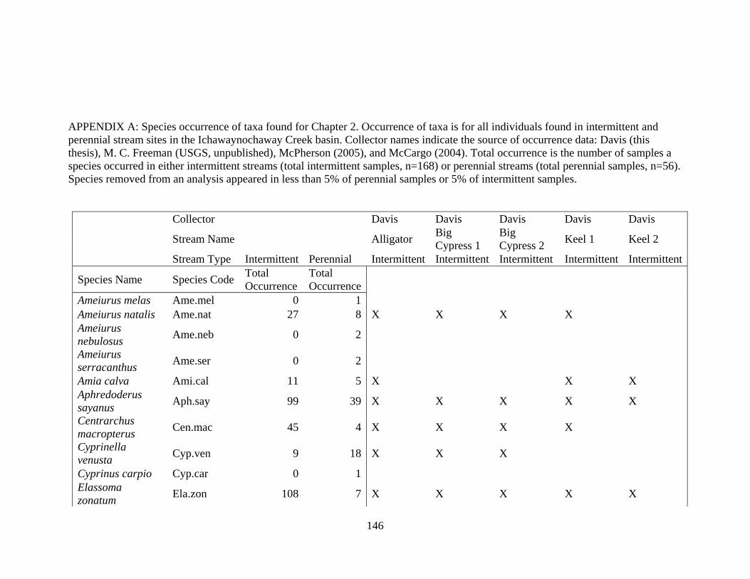
146
APPENDIX A: Species occurrence of taxa found for Chapter 2. Occurrence of taxa is for all individuals found in intermittent and
perennial stream sites in the Ichawaynochaway Creek basin. Collector names indicate the source of occurrence data: Davis (this
thesis), M. C. Freeman (USGS, unpublished), McPherson (2005), and McCargo (2004). Total occurrence is the number of samples a
species occurred in either intermittent streams (total intermittent samples, n=168) or perennial streams (total perennial samples, n=56).
Species removed from an analysis appeared in less than 5% of perennial samples or 5% of intermittent samples.
Collector Davis Davis Davis Davis Davis
Stream Name
Alligator
Big
Cypress 1
Big
Cypress 2 Keel 1 Keel 2
Stream Type Intermittent Perennial Intermittent Intermittent Intermittent Intermittent Intermittent
Species Name Species Code Total
Occurrence
Total
Occurrence
Ameiurus melas Ame.mel 0 1
Ameiurus natalis Ame.nat 27 8 X X X X
Ameiurus
nebulosus Ame.neb 0 2
Ameiurus
serracanthus Ame.ser 0 2
Amia calva Ami.cal 11 5 X
X X
Aphredoderus
sayanus Aph.say 99 39 X X X X X
Centrarchus
macropterus Cen.mac 45 4 X X X X
Cyprinella
venusta Cyp.ven 9 18 X X X
Cyprinus carpio Cyp.car 0 1
Elassoma
zonatum Ela.zon 108 7 X X X X X
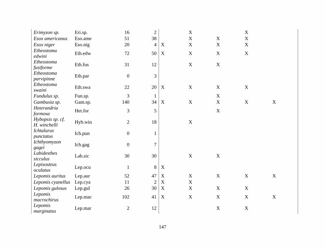
147
Erimyzon sp. Eri.sp. 16 2 X X
Esox americanus Eso.ame 51 38 X X X
Esox niger Eso.nig 20 4 X X X X
Etheostoma
edwini Eth.edw 72 50 X X X X
Etheostoma
fusiforme Eth.fus 31 12 X X
Etheostoma
parvipinne Eth.par 0 3
Etheostoma
swaini Eth.swa 22 20 X X X X
Fundulus sp. Fun.sp. 3 1 X
Gambusia sp. Gam.sp. 140 34 X X X X X
Heterandria
formosa Het.for 3 5 X
Hybopsis sp. cf.
H. winchelli Hyb.win 2 18 X
Ichtalurus
punctatus Ich.pun 0 1
Ichthyomyzon
gagei Ich.gag 0 7
Labidesthes
sicculus Lab.sic 30 30 X X
Lepisosteus
oculatus Lep.ocu 1 8 X
Lepomis auritus Lep.aur 52 47 X X X X X
Lepomis cyanellus Lep.cya 11 2 X X
Lepomis gulosus Lep.gul 26 30 X X X X
Lepomis
macrochirus Lep.mac 102 41 X X X X X
Lepomis
marginatus Lep.mar 2 12 X X
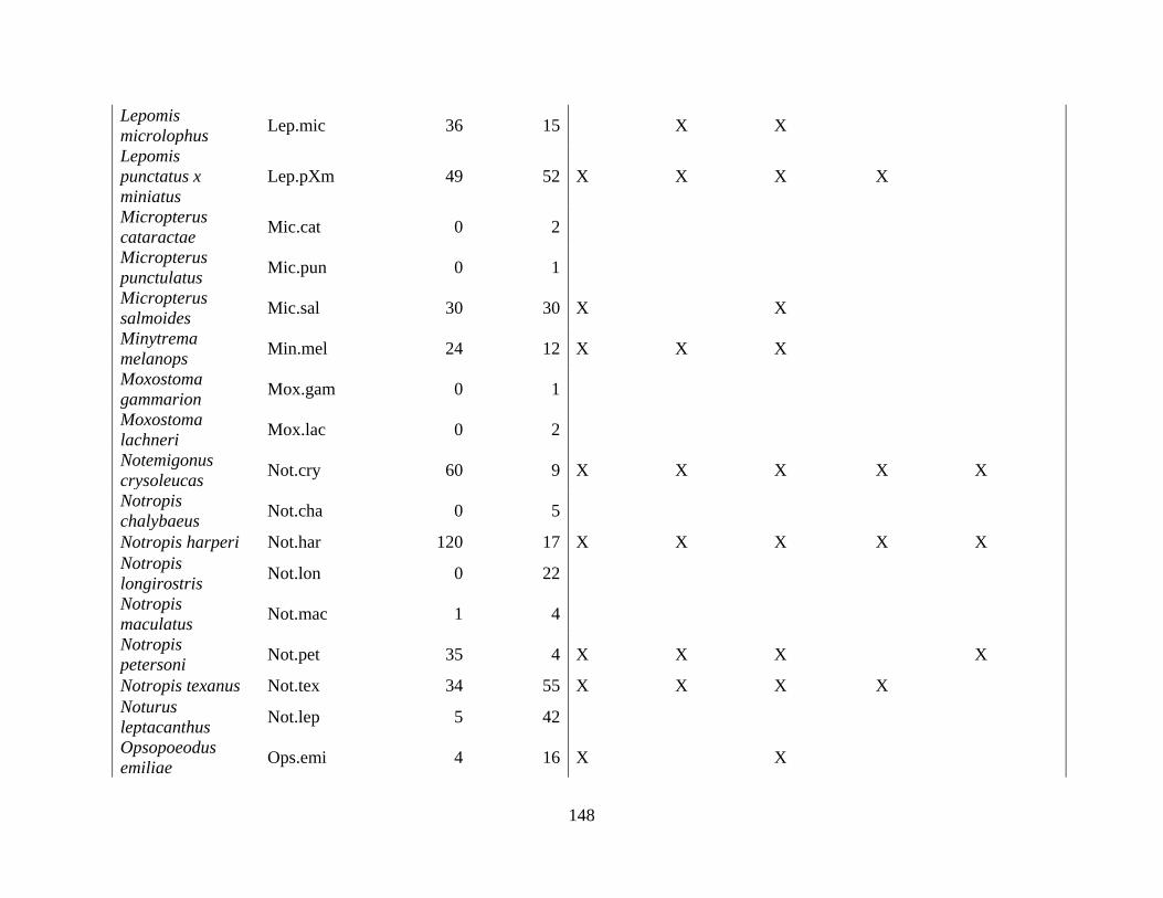
148
Lepomis
microlophus Lep.mic 36 15 X X
Lepomis
punctatus x
miniatus
Lep.pXm 49 52 X X X X
Micropterus
cataractae Mic.cat 0 2
Micropterus
punctulatus Mic.pun 0 1
Micropterus
salmoides Mic.sal 30 30 X X
Minytrema
melanops Min.mel 24 12 X X X
Moxostoma
gammarion Mox.gam 0 1
Moxostoma
lachneri Mox.lac 0 2
Notemigonus
crysoleucas Not.cry 60 9 X X X X X
Notropis
chalybaeus Not.cha 0 5
Notropis harperi Not.har 120 17 X X X X X
Notropis
longirostris Not.lon 0 22
Notropis
maculatus Not.mac 1 4
Notropis
petersoni Not.pet 35 4 X X X X
Notropis texanus Not.tex 34 55 X X X X
Noturus
leptacanthus Not.lep 5 42
Opsopoeodus
emiliae Ops.emi 4 16 X X
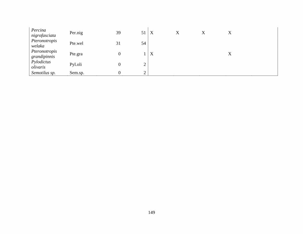
149
Percina
nigrofasciata Per.nig 39 51 X X X X
Pteronotropis
welaka Pte.wel 31 54
Pteronotropis
grandipinnis Pte.gra 0 1 X
X
Pylodictus
olivaris Pyl.oli 0 2
Semotilus sp. Sem.sp. 0 2
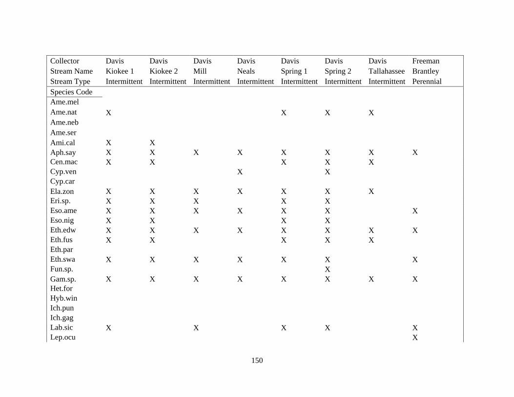
150
Collector Davis Davis Davis Davis Davis Davis Davis Freeman
Stream Name Kiokee 1 Kiokee 2 Mill Neals Spring 1 Spring 2 Tallahassee Brantley
Stream Type Intermittent Intermittent Intermittent Intermittent Intermittent Intermittent Intermittent Perennial
Species Code
Ame.mel
Ame.nat X
X X X
Ame.neb
Ame.ser
Ami.cal X X
Aph.say X X X X X X X X
Cen.mac X X
X X X
Cyp.ven
X
X
Cyp.car
Ela.zon X X X X X X X
Eri.sp. X X X X X
Eso.ame X X X X X X
X
Eso.nig X X
X X
Eth.edw X X X X X X X X
Eth.fus X X
X X X
Eth.par
Eth.swa X X X X X X
X
Fun.sp.
X
Gam.sp. X X X X X X X X
Het.for
Hyb.win
Ich.pun
Ich.gag
Lab.sic X
X X X
X
Lep.ocu
X
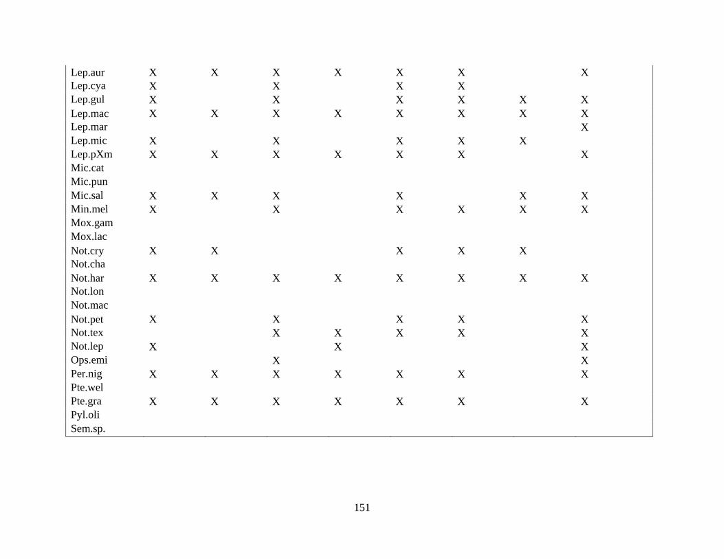
151
Lep.aur X X X X X X X
Lep.cya X X X X
Lep.gul X X X X X X
Lep.mac X X X X X X X X
Lep.mar X
Lep.mic X X X X X
Lep.pXm X X X X X X X
Mic.cat
Mic.pun
Mic.sal X X X X X X
Min.mel X X X X X X
Mox.gam
Mox.lac
Not.cry X X X X X
Not.cha
Not.har X X X X X X X X
Not.lon
Not.mac
Not.pet X X X X X
Not.tex X X X X X
Not.lep X X X
Ops.emi X X
Per.nig X X X X X X X
Pte.wel
Pte.gra X X X X X X X
Pyl.oli
Sem.sp.
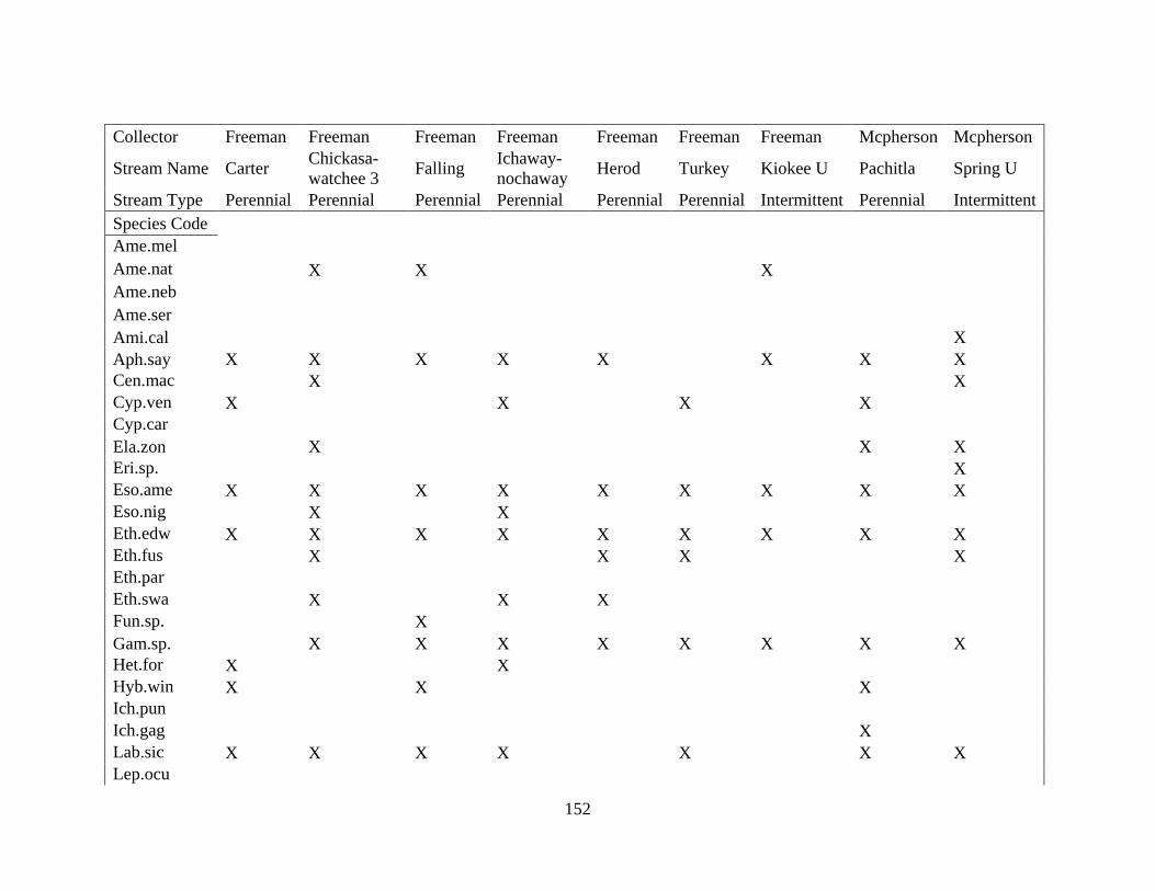
152
Collector Freeman Freeman Freeman Freeman Freeman Freeman Freeman Mcpherson Mcpherson
Stream Name Carter Chickasa-
watchee 3 Falling
Ichaway-
nochaway Herod Turkey Kiokee U Pachitla Spring U
Stream Type Perennial Perennial Perennial Perennial Perennial Perennial Intermittent Perennial Intermittent
Species Code
Ame.mel
Ame.nat X X X
Ame.neb
Ame.ser
Ami.cal X
Aph.say X X X X X X X X
Cen.mac X X
Cyp.ven X X X X
Cyp.car
Ela.zon X X X
Eri.sp. X
Eso.ame X X X X X X X X X
Eso.nig X X
Eth.edw X X X X X X X X X
Eth.fus X X X X
Eth.par
Eth.swa X X X
Fun.sp. X
Gam.sp. X X X X X X X X
Het.for X X
Hyb.win X X X
Ich.pun
Ich.gag X
Lab.sic X X X X X X X
Lep.ocu
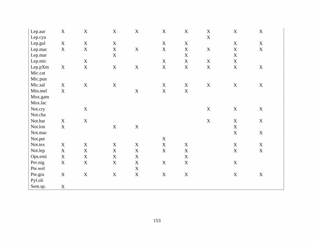
153
Lep.aur X X X X X X X X X
Lep.cya X
Lep.gul X X X X X X X
Lep.mac X X X X X X X X X
Lep.mar X X X
Lep.mic X X X X X
Lep.pXm X X X X X X X X X
Mic.cat
Mic.pun
Mic.sal X X X X X X X X
Min.mel X X X X
Mox.gam
Mox.lac
Not.cry X X X X
Not.cha
Not.har X X X X X
Not.lon X X X X
Not.mac X X
Not.pet X
Not.tex X X X X X X X X
Not.lep X X X X X X X X
Ops.emi X X X X X
Per.nig X X X X X X X
Pte.wel X
Pte.gra X X X X X X X X
Pyl.oli
Sem.sp. X
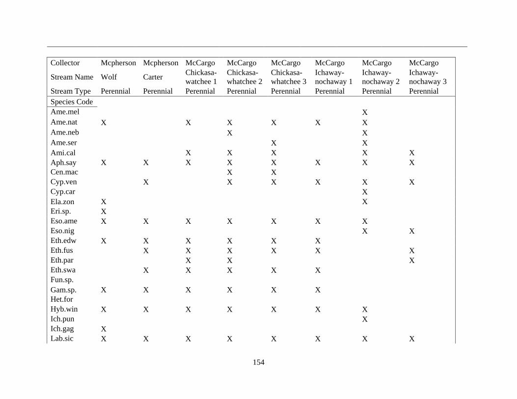
154
Collector Mcpherson Mcpherson McCargo McCargo McCargo McCargo McCargo McCargo
Stream Name Wolf Carter Chickasa-
watchee 1
Chickasa-
whatchee 2
Chickasa-
whatchee 3
Ichaway-
nochaway 1
Ichaway-
nochaway 2
Ichaway-
nochaway 3
Stream Type Perennial Perennial Perennial Perennial Perennial Perennial Perennial Perennial
Species Code
Ame.mel X
Ame.nat X X X X X X
Ame.neb X X
Ame.ser X X
Ami.cal X X X X X
Aph.say X X X X X X X X
Cen.mac X X
Cyp.ven X X X X X X
Cyp.car X
Ela.zon X X
Eri.sp. X
Eso.ame X X X X X X X
Eso.nig X X
Eth.edw X X X X X X
Eth.fus X X X X X X
Eth.par X X X
Eth.swa X X X X X
Fun.sp.
Gam.sp. X X X X X X
Het.for
Hyb.win X X X X X X X
Ich.pun X
Ich.gag X
Lab.sic X X X X X X X X
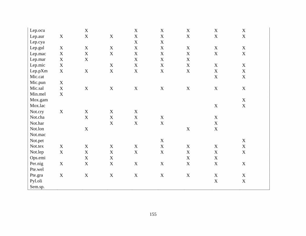
155
Lep.ocu X X X X X X
Lep.aur X X X X X X X X
Lep.cya X X
Lep.gul X X X X X X X X
Lep.mac X X X X X X X X
Lep.mar X X X X X
Lep.mic X X X X X X X
Lep.pXm X X X X X X X X
Mic.cat X X
Mic.pun X
Mic.sal X X X X X X X X
Min.mel X
Mox.gam X
Mox.lac X X
Not.cry X X X X
Not.cha X X X X X
Not.har X X X X
Not.lon X X X
Not.mac
Not.pet X X
Not.tex X X X X X X X X
Not.lep X X X X X X X X
Ops.emi X X X X
Per.nig X X X X X X X X
Pte.wel
Pte.gra X X X X X X X X
Pyl.oli X X
Sem.sp.

156
References:
McCargo, J. W. 2004. Influence of drought of seasonal fish assemblages and habitat in the lower
Flint River Basin, Georgia. University of Georgia, Masters Thesis.
McPherson, R. D., Jr. 2005. An assessment of fish community structure and seasonal habitat use
of headwater confined channels and headwater wetlands in the lower Flint River Basin,
southwest Georgia. University of Georgia, Masters Thesis.
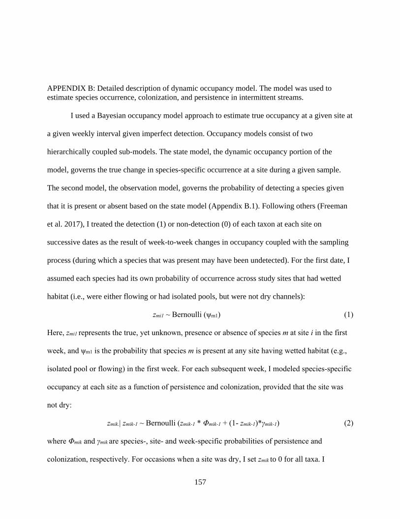
157
APPENDIX B: Detailed description of dynamic occupancy model. The model was used to
estimate species occurrence, colonization, and persistence in intermittent streams.
I used a Bayesian occupancy model approach to estimate true occupancy at a given site at
a given weekly interval given imperfect detection. Occupancy models consist of two
hierarchically coupled sub-models. The state model, the dynamic occupancy portion of the
model, governs the true change in species-specific occurrence at a site during a given sample.
The second model, the observation model, governs the probability of detecting a species given
that it is present or absent based on the state model (Appendix B.1). Following others (Freeman
et al. 2017), I treated the detection (1) or non-detection (0) of each taxon at each site on
successive dates as the result of week-to-week changes in occupancy coupled with the sampling
process (during which a species that was present may have been undetected). For the first date, I
assumed each species had its own probability of occurrence across study sites that had wetted
habitat (i.e., were either flowing or had isolated pools, but were not dry channels):
zmi1 ~ Bernoulli (ψm1) (1)
Here, zmi1 represents the true, yet unknown, presence or absence of species m at site i in the first
week, and ψm1 is the probability that species m is present at any site having wetted habitat (e.g.,
isolated pool or flowing) in the first week. For each subsequent week, I modeled species-specific
occupancy at each site as a function of persistence and colonization, provided that the site was
not dry:
zmik.| zmik-1 ~ Bernoulli (zmik-1 * Φmik-1 + (1- zmik-1)*γmik-1) (2)
where Φmik and γmik are species-, site- and week-specific probabilities of persistence and
colonization, respectively. For occasions when a site was dry, I set zmik to 0 for all taxa. I

158
modeled the actual detection (1) or non-detection (0) of each of the m species in the jth replicate
reach at site i in week k as:
ymijk | zmik ~ Bernoulli (zmik * pmijk) (3)
where pmik is the species- and sample-specific probability of detecting species m, given that
species m was present (zmik = 1).
I used this model to evaluate the evidence that species more commonly found in
intermittent streams in fact had either higher persistence when streams dried to isolated pools, or
recolonized more quickly when streams resumed flowing, than species that were more
commonly found in perennial streams (or than species that were not characteristic of either
stream type). For these analyses, I characterized flow condition during each interval between
sampling dates, at each site, as: (1) flowing on both dates (flowing to flowing); (2) flowing to
isolated (or vise versa); (3) isolated on both dates (isolated to isolated); (4) and if an isolated pool
is open to upstream or downstream movement (“isolated-open” to isolated-open” or “flowing to
isolated-open”) (Figure 2.3).
I then used site- and interval-specific flow condition, and species type (“intermittent”,
“perennial”, or “other”) as interacting covariates on fish persistence and colonization. I fit
covariates using a logit-link. The model for persistence was:
logit(Φmik ) = mean.phim + beta.phi.weeks.slackm*weeks.slackik + (4)
beta.phi.close.openm*isolated.openik + epsilon.phi.site.dateik
where, isolated.openik is equal to 1 if site i during interval k experienced conditions of “isolated
to isolated-open” or “flowing to isolated-open” and 0 otherwise. The term weeks.slackik was set
to 0 unless site i during interval k was dried to isolated pools, in which case weeks.slackik was the
number of successive weeks that I observed the site to have been in that state. I assumed that the
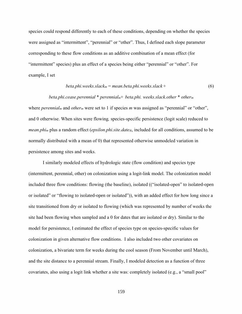
159
species could respond differently to each of these conditions, depending on whether the species
were assigned as “intermittent”, “perennial” or “other”. Thus, I defined each slope parameter
corresponding to these flow conditions as an additive combination of a mean effect (for
“intermittent” species) plus an effect of a species being either “perennial” or “other”. For
example, I set
beta.phi.weeks.slackm = mean.beta.phi.weeks.slack + (6)
beta.phi.cease.perennial * perennialm+ beta.phi. weeks.slack.other * otherm
where perennialm and otherm were set to 1 if species m was assigned as “perennial” or “other”,
and 0 otherwise. When sites were flowing, species-specific persistence (logit scale) reduced to
mean.phim plus a random effect (epsilon.phi.site.dateik, included for all conditions, assumed to be
normally distributed with a mean of 0) that represented otherwise unmodeled variation in
persistence among sites and weeks.
I similarly modeled effects of hydrologic state (flow condition) and species type
(intermittent, perennial, other) on colonization using a logit-link model. The colonization model
included three flow conditions: flowing (the baseline), isolated ((“isolated-open” to isolated-open
or isolated” or “flowing to isolated-open or isolated”)), with an added effect for how long since a
site transitioned from dry or isolated to flowing (which was represented by number of weeks the
site had been flowing when sampled and a 0 for dates that are isolated or dry). Similar to the
model for persistence, I estimated the effect of species type on species-specific values for
colonization in given alternative flow conditions. I also included two other covariates on
colonization, a bivariate term for weeks during the cool season (From November until March),
and the site distance to a perennial stream. Finally, I modeled detection as a function of three
covariates, also using a logit link whether a site was: completely isolated (e.g., a “small pool”
160
closed from any upstream or downstream movement); isolated-open (e.g., a “big pool” open to
upstream or downstream movement); and whether a stream was sampled with only an upstream
pass, or both an upstream and a downstream pass.
I modeled occupancy dynamics for adults and juveniles separately to evaluate evidence
that younger fish had higher persistence, or colonization, rates than adults. For each analysis, I
created a four-dimensional matrix of 21 species (model for adults including all taxa that occurred
in at least 5% of samples; 25 in the case of juveniles, Appendix C), by 12 sites, by two replicate
reaches sampled on each date, by 82 weekly samples (spanning June 2015 to January 2017).
Occasions when sites were not sampled in a particular week were coded as “NA”, as was the
second replicate on dates when I only sampled isolated pools at a site. I fit models with a
Bayesian framework implemented with the Markov chain Monte Carlo (MCMC) software JAGS
version 4.3.0 (Plummer 2003), run using the R package “jagsUI” (Kellner 2015) in R version
3.4.1 (R Core Team 2014). I used diffuse priors for parameter coefficients and ran three chains
for 30,000 iterations, thinned by four, after a burn-in of 3,000. I assessed convergence using the
Brooks-Gelman-Rubin statistic, R-hat (Brooks and Gelman 1998). I assessed model fit with a
Bayesian p-value for based on the discrepancy (Freeman-Tukey statistic) between the observed
and (model-based) expected number of species detected in each survey, and the same statistic
calculated for a replicate data set simulated using persistence, colonization, and detection
estimates at each MCMC iterations (Schaub and Kéry 2012). The Bayesian p-value was the
proportion of summed discrepancy values for the simulated data that exceeded the same for the
observed data. A value of less than about 0.05 or greater than about 0.95 would indicate
substantial model lack-of-fit (Schaub and Kéry 2012).
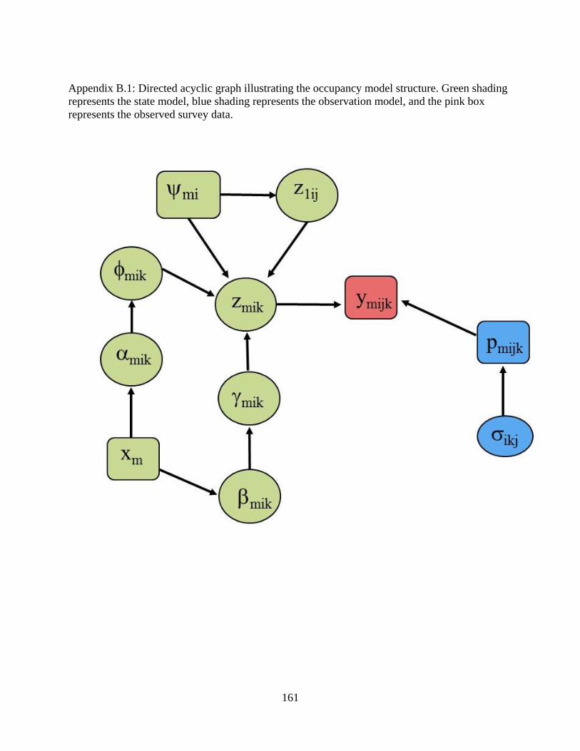
161
Appendix B.1: Directed acyclic graph illustrating the occupancy model structure. Green shading
represents the state model, blue shading represents the observation model, and the pink box
represents the observed survey data.
162
Refereces:
Brooks, S. P., and A. Gelman. 1998. General methods for monitoring convergence of iterative
simulations. Journal of Computational and Graphical Statistics 7:434-455.
Freeman, M. C., M. M. Hagler, P. M. Bumpers, K. Wheeler, S. Wenger, and B. Freeman. 2017.
Long-term monitoring data provide evidence of declining species richness in a river
valued for biodiversity conservation. Journal of Fish and Wildlife Management. 2017 in
press.
Kellner, K. 2015. jagsUI: a wrapper around rjags to streamline JAGS analyses. R package
version 1.
Plummer, M. 2003. JAGS: A program for analysis of Bayesian graphical models using Gibbs
sampling. Proceedings of the 3rd International workshop on distributed statistical
computing. Vienna, Austria.
R Core Team. 2014. R: A language and environment for statistical computing. Vienna, Austria:
R Foundation for Statistical Computing. Available: http://cran.rproject.org (June 2017).
Schaub, M., and M. Kéry. 2012. Combining information in hierarchical models improves
inferences in population ecology and demographic population analyses. Animal
Conservation 15:125-126.
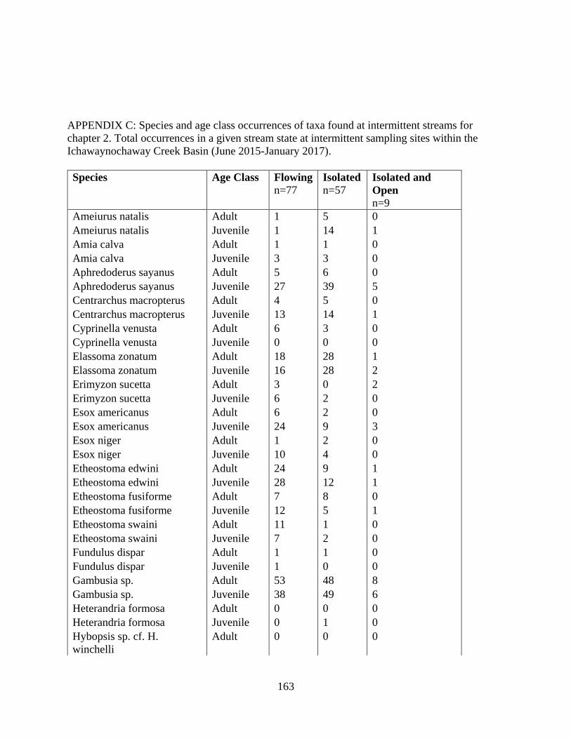
163
APPENDIX C: Species and age class occurrences of taxa found at intermittent streams for
chapter 2. Total occurrences in a given stream state at intermittent sampling sites within the
Ichawaynochaway Creek Basin (June 2015-January 2017).
Species Age Class Flowing
n=77
Isolated
n=57
Isolated and
Open
n=9
Ameiurus natalis Adult 1 5 0
Ameiurus natalis Juvenile 1 14 1
Amia calva Adult 1 1 0
Amia calva Juvenile 3 3 0
Aphredoderus sayanus Adult 5 6 0
Aphredoderus sayanus Juvenile 27 39 5
Centrarchus macropterus Adult 4 5 0
Centrarchus macropterus Juvenile 13 14 1
Cyprinella venusta Adult 6 3 0
Cyprinella venusta Juvenile 0 0 0
Elassoma zonatum Adult 18 28 1
Elassoma zonatum Juvenile 16 28 2
Erimyzon sucetta Adult 3 0 2
Erimyzon sucetta Juvenile 6 2 0
Esox americanus Adult 6 2 0
Esox americanus Juvenile 24 9 3
Esox niger Adult 1 2 0
Esox niger Juvenile 10 4 0
Etheostoma edwini Adult 24 9 1
Etheostoma edwini Juvenile 28 12 1
Etheostoma fusiforme Adult 7 8 0
Etheostoma fusiforme Juvenile 12 5 1
Etheostoma swaini Adult 11 1 0
Etheostoma swaini Juvenile 7 2 0
Fundulus dispar Adult 1 1 0
Fundulus dispar Juvenile 1 0 0
Gambusia sp. Adult 53 48 8
Gambusia sp. Juvenile 38 49 6
Heterandria formosa Adult 0 0 0
Heterandria formosa Juvenile 0 1 0
Hybopsis sp. cf. H.
winchelli
Adult 0 0 0
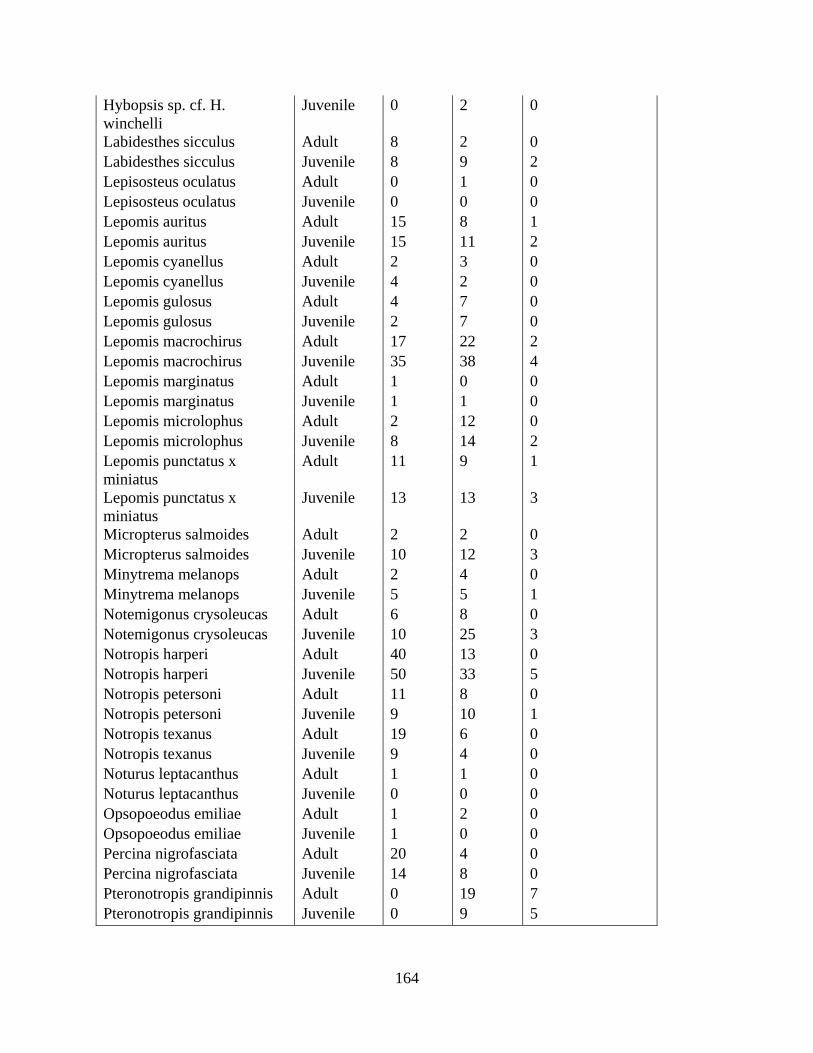
164
Hybopsis sp. cf. H.
winchelli
Juvenile 0 2 0
Labidesthes sicculus Adult 8 2 0
Labidesthes sicculus Juvenile 8 9 2
Lepisosteus oculatus Adult 0 1 0
Lepisosteus oculatus Juvenile 0 0 0
Lepomis auritus Adult 15 8 1
Lepomis auritus Juvenile 15 11 2
Lepomis cyanellus Adult 2 3 0
Lepomis cyanellus Juvenile 4 2 0
Lepomis gulosus Adult 4 7 0
Lepomis gulosus Juvenile 2 7 0
Lepomis macrochirus Adult 17 22 2
Lepomis macrochirus Juvenile 35 38 4
Lepomis marginatus Adult 1 0 0
Lepomis marginatus Juvenile 1 1 0
Lepomis microlophus Adult 2 12 0
Lepomis microlophus Juvenile 8 14 2
Lepomis punctatus x
miniatus
Adult 11 9 1
Lepomis punctatus x
miniatus
Juvenile 13 13 3
Micropterus salmoides Adult 2 2 0
Micropterus salmoides Juvenile 10 12 3
Minytrema melanops Adult 2 4 0
Minytrema melanops Juvenile 5 5 1
Notemigonus crysoleucas Adult 6 8 0
Notemigonus crysoleucas Juvenile 10 25 3
Notropis harperi Adult 40 13 0
Notropis harperi Juvenile 50 33 5
Notropis petersoni Adult 11 8 0
Notropis petersoni Juvenile 9 10 1
Notropis texanus Adult 19 6 0
Notropis texanus Juvenile 9 4 0
Noturus leptacanthus Adult 1 1 0
Noturus leptacanthus Juvenile 0 0 0
Opsopoeodus emiliae Adult 1 2 0
Opsopoeodus emiliae Juvenile 1 0 0
Percina nigrofasciata Adult 20 4 0
Percina nigrofasciata Juvenile 14 8 0
Pteronotropis grandipinnis Adult 0 19 7
Pteronotropis grandipinnis Juvenile 0 9 5
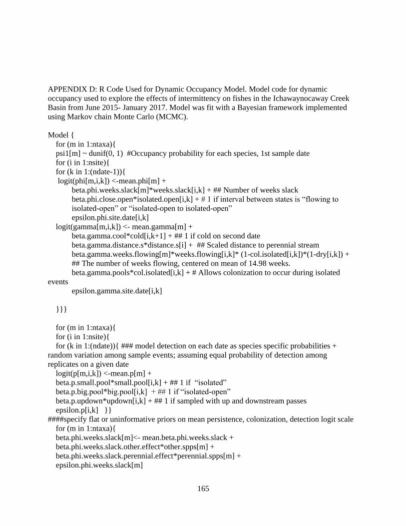
165
APPENDIX D: R Code Used for Dynamic Occupancy Model. Model code for dynamic
occupancy used to explore the effects of intermittency on fishes in the Ichawaynocaway Creek
Basin from June 2015- January 2017. Model was fit with a Bayesian framework implemented
using Markov chain Monte Carlo (MCMC).
Model {
for (m in 1:ntaxa){
psi1[m] ~ dunif(0, 1) #Occupancy probability for each species, 1st sample date
for (i in 1:nsite){
for (k in 1:(ndate-1)){
logit(phi[m,i,k]) <-mean.phi[m] +
beta.phi.weeks.slack[m]*weeks.slack[i,k] + ## Number of weeks slack
beta.phi.close.open*isolated.open[i,k] + # 1 if interval between states is “flowing to
isolated-open” or “isolated-open to isolated-open”
epsilon.phi.site.date[i,k]
logit(gamma[m,i,k]) <- mean.gamma[m] +
beta.gamma.cool*cold[i,k+1] + ## 1 if cold on second date
beta.gamma.distance.s*distance.s[i] + ## Scaled distance to perennial stream
beta.gamma.weeks.flowing[m]*weeks.flowing[i,k]* (1-col.isolated[i,k])*(1-dry[i,k]) +
## The number of weeks flowing, centered on mean of 14.98 weeks.
beta.gamma.pools*col.isolated[i,k] + # Allows colonization to occur during isolated
events
epsilon.gamma.site.date[i,k]
}}}
for (m in 1:ntaxa){
for (i in 1:nsite){
for (k in 1:(ndate)){ ### model detection on each date as species specific probabilities +
random variation among sample events; assuming equal probability of detection among
replicates on a given date
logit(p[m,i,k]) <-mean.p[m] +
beta.p.small.pool*small.pool[i,k] + ## 1 if “isolated”
beta.p.big.pool*big.pool[i,k] + ## 1 if “isolated-open”
beta.p.updown*updown[i,k] + ## 1 if sampled with up and downstream passes
epsilon.p[i,k] }}
####specify flat or uninformative priors on mean persistence, colonization, detection logit scale
for (m in 1:ntaxa){
beta.phi.weeks.slack[m]<- mean.beta.phi.weeks.slack +
beta.phi.weeks.slack.other.effect*other.spps[m] +
beta.phi.weeks.slack.perennial.effect*perennial.spps[m] +
epsilon.phi.weeks.slack[m]
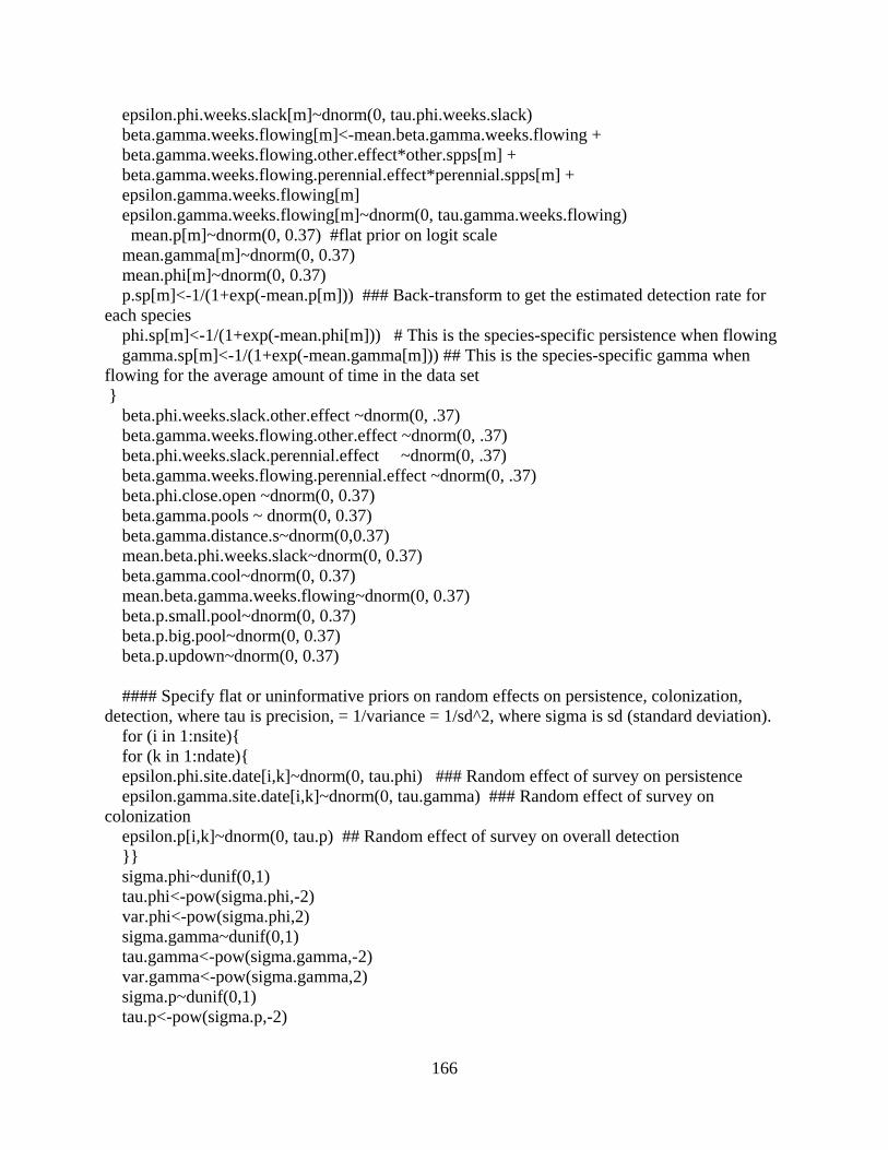
166
epsilon.phi.weeks.slack[m]~dnorm(0, tau.phi.weeks.slack)
beta.gamma.weeks.flowing[m]<-mean.beta.gamma.weeks.flowing +
beta.gamma.weeks.flowing.other.effect*other.spps[m] +
beta.gamma.weeks.flowing.perennial.effect*perennial.spps[m] +
epsilon.gamma.weeks.flowing[m]
epsilon.gamma.weeks.flowing[m]~dnorm(0, tau.gamma.weeks.flowing)
mean.p[m]~dnorm(0, 0.37) #flat prior on logit scale
mean.gamma[m]~dnorm(0, 0.37)
mean.phi[m]~dnorm(0, 0.37)
p.sp[m]<-1/(1+exp(-mean.p[m])) ### Back-transform to get the estimated detection rate for
each species
phi.sp[m]<-1/(1+exp(-mean.phi[m])) # This is the species-specific persistence when flowing
gamma.sp[m]<-1/(1+exp(-mean.gamma[m])) ## This is the species-specific gamma when
flowing for the average amount of time in the data set
}
beta.phi.weeks.slack.other.effect ~dnorm(0, .37)
beta.gamma.weeks.flowing.other.effect ~dnorm(0, .37)
beta.phi.weeks.slack.perennial.effect ~dnorm(0, .37)
beta.gamma.weeks.flowing.perennial.effect ~dnorm(0, .37)
beta.phi.close.open ~dnorm(0, 0.37)
beta.gamma.pools ~ dnorm(0, 0.37)
beta.gamma.distance.s~dnorm(0,0.37)
mean.beta.phi.weeks.slack~dnorm(0, 0.37)
beta.gamma.cool~dnorm(0, 0.37)
mean.beta.gamma.weeks.flowing~dnorm(0, 0.37)
beta.p.small.pool~dnorm(0, 0.37)
beta.p.big.pool~dnorm(0, 0.37)
beta.p.updown~dnorm(0, 0.37)
#### Specify flat or uninformative priors on random effects on persistence, colonization,
detection, where tau is precision, = 1/variance = 1/sd^2, where sigma is sd (standard deviation).
for (i in 1:nsite){
for (k in 1:ndate){
epsilon.phi.site.date[i,k]~dnorm(0, tau.phi) ### Random effect of survey on persistence
epsilon.gamma.site.date[i,k]~dnorm(0, tau.gamma) ### Random effect of survey on
colonization
epsilon.p[i,k]~dnorm(0, tau.p) ## Random effect of survey on overall detection
}}
sigma.phi~dunif(0,1)
tau.phi<-pow(sigma.phi,-2)
var.phi<-pow(sigma.phi,2)
sigma.gamma~dunif(0,1)
tau.gamma<-pow(sigma.gamma,-2)
var.gamma<-pow(sigma.gamma,2)
sigma.p~dunif(0,1)
tau.p<-pow(sigma.p,-2)
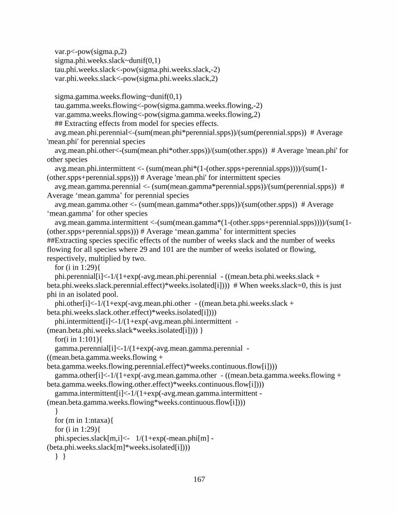
167
var.p<-pow(sigma.p,2)
sigma.phi.weeks.slack~dunif(0,1)
tau.phi.weeks.slack<-pow(sigma.phi.weeks.slack,-2)
var.phi.weeks.slack<-pow(sigma.phi.weeks.slack,2)
sigma.gamma.weeks.flowing~dunif(0,1)
tau.gamma.weeks.flowing<-pow(sigma.gamma.weeks.flowing,-2)
var.gamma.weeks.flowing<-pow(sigma.gamma.weeks.flowing,2)
## Extracting effects from model for species effects.
avg.mean.phi.perennial<-(sum(mean.phi*perennial.spps))/(sum(perennial.spps)) # Average
'mean.phi' for perennial species
avg.mean.phi.other<-(sum(mean.phi*other.spps))/(sum(other.spps)) # Average 'mean.phi' for
other species
avg.mean.phi.intermittent <- (sum(mean.phi*(1-(other.spps+perennial.spps))))/(sum(1-
(other.spps+perennial.spps))) # Average 'mean.phi' for intermittent species
avg.mean.gamma.perennial <- (sum(mean.gamma*perennial.spps))/(sum(perennial.spps)) #
Average ‘mean.gamma’ for perennial species
avg.mean.gamma.other <- (sum(mean.gamma*other.spps))/(sum(other.spps)) # Average
‘mean.gamma’ for other species
avg.mean.gamma.intermittent <-(sum(mean.gamma*(1-(other.spps+perennial.spps))))/(sum(1-
(other.spps+perennial.spps))) # Average ‘mean.gamma’ for intermittent species
##Extracting species specific effects of the number of weeks slack and the number of weeks
flowing for all species where 29 and 101 are the number of weeks isolated or flowing,
respectively, multiplied by two.
for (i in 1:29){
phi.perennial[i]<-1/(1+exp(-avg.mean.phi.perennial - ((mean.beta.phi.weeks.slack +
beta.phi.weeks.slack.perennial.effect)*weeks.isolated[i]))) # When weeks.slack=0, this is just
phi in an isolated pool.
phi.other[i]<-1/(1+exp(-avg.mean.phi.other - ((mean.beta.phi.weeks.slack +
beta.phi.weeks.slack.other.effect)*weeks.isolated[i])))
phi.intermittent[i]<-1/(1+exp(-avg.mean.phi.intermittent -
(mean.beta.phi.weeks.slack*weeks.isolated[i]))) }
for(i in 1:101){
gamma.perennial[i]<-1/(1+exp(-avg.mean.gamma.perennial -
((mean.beta.gamma.weeks.flowing +
beta.gamma.weeks.flowing.perennial.effect)*weeks.continuous.flow[i])))
gamma.other[i]<-1/(1+exp(-avg.mean.gamma.other - ((mean.beta.gamma.weeks.flowing +
beta.gamma.weeks.flowing.other.effect)*weeks.continuous.flow[i])))
gamma.intermittent[i]<-1/(1+exp(-avg.mean.gamma.intermittent -
(mean.beta.gamma.weeks.flowing*weeks.continuous.flow[i])))
}
for (m in 1:ntaxa){
for (i in 1:29){
phi.species.slack[m,i]<- 1/(1+exp(-mean.phi[m] -
(beta.phi.weeks.slack[m]*weeks.isolated[i])))
} }
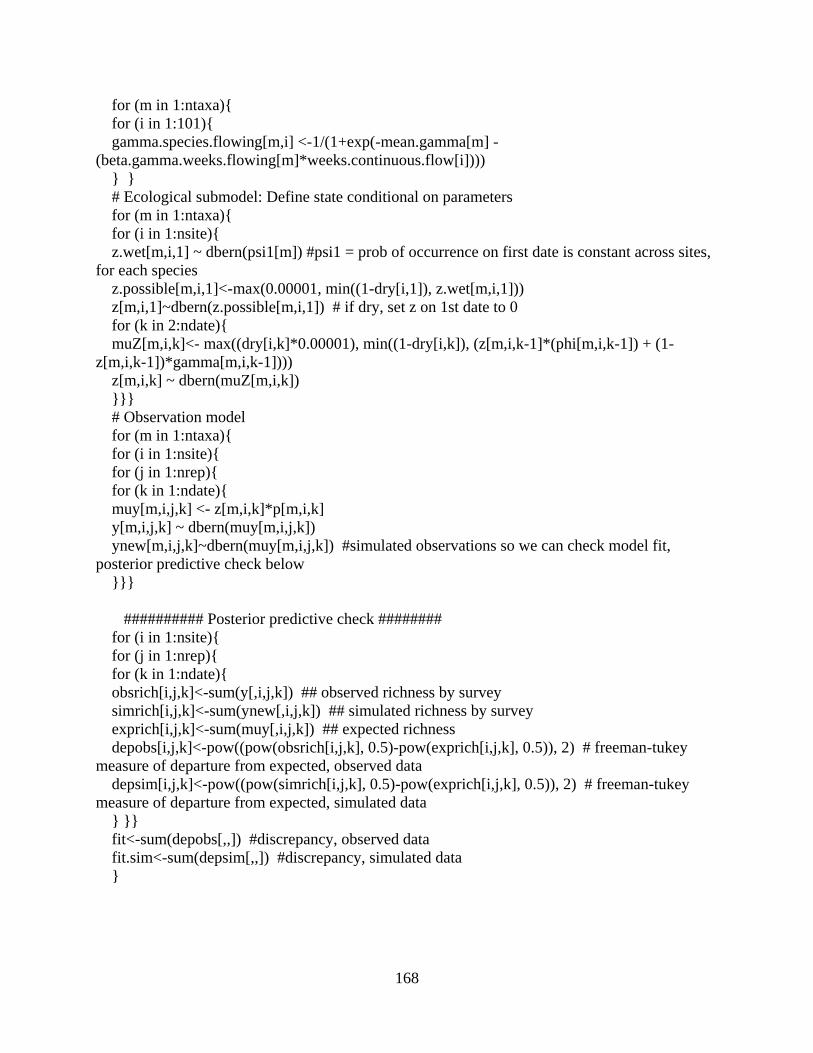
168
for (m in 1:ntaxa){
for (i in 1:101){
gamma.species.flowing[m,i] <-1/(1+exp(-mean.gamma[m] -
(beta.gamma.weeks.flowing[m]*weeks.continuous.flow[i])))
} }
# Ecological submodel: Define state conditional on parameters
for (m in 1:ntaxa){
for (i in 1:nsite){
z.wet[m,i,1] ~ dbern(psi1[m]) #psi1 = prob of occurrence on first date is constant across sites,
for each species
z.possible[m,i,1]<-max(0.00001, min((1-dry[i,1]), z.wet[m,i,1]))
z[m,i,1]~dbern(z.possible[m,i,1]) # if dry, set z on 1st date to 0
for (k in 2:ndate){
muZ[m,i,k]<- max((dry[i,k]*0.00001), min((1-dry[i,k]), (z[m,i,k-1]*(phi[m,i,k-1]) + (1-
z[m,i,k-1])*gamma[m,i,k-1])))
z[m,i,k] ~ dbern(muZ[m,i,k])
}}}
# Observation model
for (m in 1:ntaxa){
for (i in 1:nsite){
for (j in 1:nrep){
for (k in 1:ndate){
muy[m,i,j,k] <- z[m,i,k]*p[m,i,k]
y[m,i,j,k] ~ dbern(muy[m,i,j,k])
ynew[m,i,j,k]~dbern(muy[m,i,j,k]) #simulated observations so we can check model fit,
posterior predictive check below
}}}
########## Posterior predictive check ########
for (i in 1:nsite){
for (j in 1:nrep){
for (k in 1:ndate){
obsrich[i,j,k]<-sum(y[,i,j,k]) ## observed richness by survey
simrich[i,j,k]<-sum(ynew[,i,j,k]) ## simulated richness by survey
exprich[i,j,k]<-sum(muy[,i,j,k]) ## expected richness
depobs[i,j,k]<-pow((pow(obsrich[i,j,k], 0.5)-pow(exprich[i,j,k], 0.5)), 2) # freeman-tukey
measure of departure from expected, observed data
depsim[i,j,k]<-pow((pow(simrich[i,j,k], 0.5)-pow(exprich[i,j,k], 0.5)), 2) # freeman-tukey
measure of departure from expected, simulated data
} }}
fit<-sum(depobs[,,]) #discrepancy, observed data
fit.sim<-sum(depsim[,,]) #discrepancy, simulated data
}
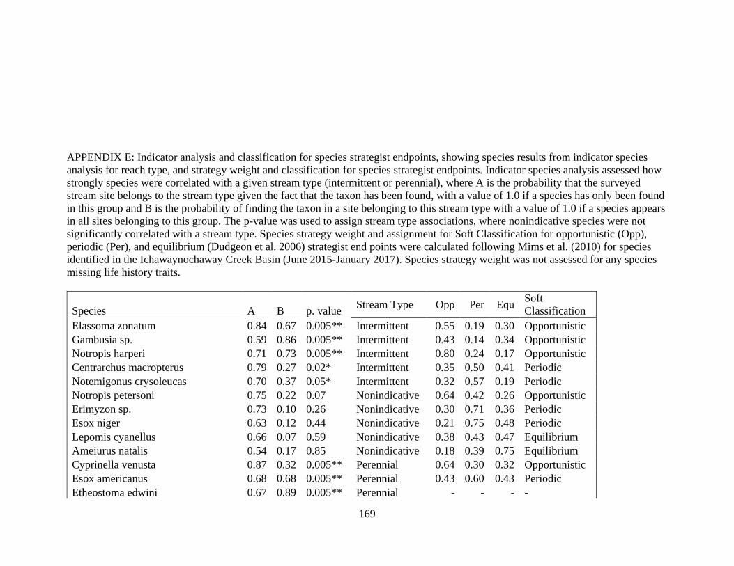
169
APPENDIX E: Indicator analysis and classification for species strategist endpoints, showing species results from indicator species
analysis for reach type, and strategy weight and classification for species strategist endpoints. Indicator species analysis assessed how
strongly species were correlated with a given stream type (intermittent or perennial), where A is the probability that the surveyed
stream site belongs to the stream type given the fact that the taxon has been found, with a value of 1.0 if a species has only been found
in this group and B is the probability of finding the taxon in a site belonging to this stream type with a value of 1.0 if a species appears
in all sites belonging to this group. The p-value was used to assign stream type associations, where nonindicative species were not
significantly correlated with a stream type. Species strategy weight and assignment for Soft Classification for opportunistic (Opp),
periodic (Per), and equilibrium (Dudgeon et al. 2006) strategist end points were calculated following Mims et al. (2010) for species
identified in the Ichawaynochaway Creek Basin (June 2015-January 2017). Species strategy weight was not assessed for any species
missing life history traits.
Species A B p. value Stream Type Opp Per Equ
Soft
Classification
Elassoma zonatum 0.84 0.67 0.005** Intermittent 0.55 0.19 0.30 Opportunistic
Gambusia sp. 0.59 0.86 0.005** Intermittent 0.43 0.14 0.34 Opportunistic
Notropis harperi 0.71 0.73 0.005** Intermittent 0.80 0.24 0.17 Opportunistic
Centrarchus macropterus 0.79 0.27 0.02* Intermittent 0.35 0.50 0.41 Periodic
Notemigonus crysoleucas 0.70 0.37 0.05* Intermittent 0.32 0.57 0.19 Periodic
Notropis petersoni 0.75 0.22 0.07 Nonindicative 0.64 0.42 0.26 Opportunistic
Erimyzon sp. 0.73 0.10 0.26 Nonindicative 0.30 0.71 0.36 Periodic
Esox niger 0.63 0.12 0.44 Nonindicative 0.21 0.75 0.48 Periodic
Lepomis cyanellus 0.66 0.07 0.59 Nonindicative 0.38 0.43 0.47 Equilibrium
Ameiurus natalis 0.54 0.17 0.85 Nonindicative 0.18 0.39 0.75 Equilibrium
Cyprinella venusta 0.87 0.32 0.005** Perennial 0.64 0.30 0.32 Opportunistic
Esox americanus 0.68 0.68 0.005** Perennial 0.43 0.60 0.43 Periodic
Etheostoma edwini 0.67 0.89 0.005** Perennial - - - -
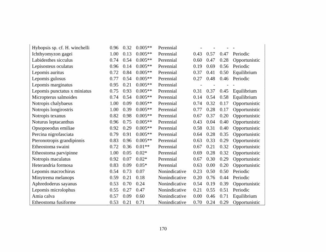
170
Hybopsis sp. cf. H. winchelli 0.96 0.32 0.005** Perennial - - - -
Ichthyomyzon gagei 1.00 0.13 0.005** Perennial 0.43 0.57 0.47 Periodic
Labidesthes sicculus 0.74 0.54 0.005** Perennial 0.60 0.47 0.28 Opportunistic
Lepisosteus oculatus 0.96 0.14 0.005** Perennial 0.19 0.69 0.56 Periodic
Lepomis auritus 0.72 0.84 0.005** Perennial 0.37 0.41 0.50 Equilibrium
Lepomis gulosus 0.77 0.54 0.005** Perennial 0.27 0.48 0.46 Periodic
Lepomis marginatus 0.95 0.21 0.005** Perennial - - - -
Lepomis punctatus x miniatus 0.75 0.93 0.005** Perennial 0.31 0.37 0.45 Equilibrium
Micropterus salmoides 0.74 0.54 0.005** Perennial 0.14 0.54 0.58 Equilibrium
Notropis chalybaeus 1.00 0.09 0.005** Perennial 0.74 0.32 0.17 Opportunistic
Notropis longirostris 1.00 0.39 0.005** Perennial 0.77 0.28 0.17 Opportunistic
Notropis texanus 0.82 0.98 0.005** Perennial 0.67 0.37 0.20 Opportunistic
Noturus leptacanthus 0.96 0.75 0.005** Perennial 0.43 0.04 0.40 Opportunistic
Opsopoeodus emiliae 0.92 0.29 0.005** Perennial 0.58 0.31 0.40 Opportunistic
Percina nigrofasciata 0.79 0.91 0.005** Perennial 0.64 0.28 0.35 Opportunistic
Pteronotropis grandipinnis 0.83 0.96 0.005** Perennial 0.63 0.33 0.29 Opportunistic
Etheostoma swaini 0.72 0.36 0.01** Perennial 0.67 0.21 0.32 Opportunistic
Etheostoma parvipinne 1.00 0.05 0.02* Perennial 0.69 0.28 0.32 Opportunistic
Notropis maculatus 0.92 0.07 0.02* Perennial 0.67 0.30 0.29 Opportunistic
Heterandria formosa 0.83 0.09 0.05* Perennial 0.63 0.00 0.20 Opportunistic
Lepomis macrochirus 0.54 0.73 0.07 Nonindicative 0.23 0.50 0.50 Periodic
Minytrema melanops 0.59 0.21 0.18 Nonindicative 0.20 0.76 0.44 Periodic
Aphredoderus sayanus 0.53 0.70 0.24 Nonindicative 0.54 0.19 0.39 Opportunistic
Lepomis microlophus 0.55 0.27 0.47 Nonindicative 0.21 0.55 0.51 Periodic
Amia calva 0.57 0.09 0.60 Nonindicative 0.00 0.46 0.71 Equilibrium
Etheostoma fusiforme 0.53 0.21 0.71 Nonindicative 0.70 0.24 0.29 Opportunistic

171
References:
Dudgeon, D., A. H. Arthington, M. O. Gessner, Z. Kawabata, D. J. Knowler, C. Leveque,
R. J. Naiman, A. H. Prieur-Richard, D. Soto, M. L. Stiassny, and C. A. Sullivan.
2006. Freshwater biodiversity: importance, threats, status and conservation
challenges. Biological Reviews of the Cambridge Philosophical Society 81:163-
182.
Mims, M. C., J. D. Olden, Z. R. Shattuck, and N. L. Poff. 2010. Life history trait
diversity of native freshwater fishes in North America. Ecology of Freshwater
Fish 19:390-400.


