Streaking artifact reduction for quantitativesusceptibility mapping of sources with largedynamic rangeHongjiang Weia, Russell Dibbb, Yan Zhouc, Yawen Sunc, Jianrong Xuc,Nian Wanga and Chunlei Liua,d*

Quantitative susceptibility mapping (QSM) is a novel MRI technique for the measurement of tissue magnetic sus-ceptibility in three dimensions. Although numerous algorithms have been developed to solve this ill-posed in-verse problem, the estimation of susceptibility maps with a wide range of values is still problematic. In casessuch as large veins, contrast agent uptake and intracranial hemorrhages, extreme susceptibility values in focalareas cause severe streaking artifacts. To enable the reduction of these artifacts, whilst preserving subtle suscep-tibility contrast, a two-level QSM reconstruction algorithm (streaking artifact reduction for QSM, STAR-QSM) wasdeveloped in this study by tuning a regularization parameter to automatically reconstruct both large and smallsusceptibility values. Compared with current state-of-the-art QSM methods, such as the improved sparse linearequation and least-squares (iLSQR) algorithm, STAR-QSM significantly reduced the streaking artifacts, whilst pre-serving the sharp boundaries for blood vessels of mouse brains in vivo and fine anatomical details of high-resolution mouse brains ex vivo. Brain image data from patients with cerebral hematoma and multiple sclerosisfurther illustrated the superiority of this method in reducing streaking artifacts caused by large susceptibilitysources, whilst maintaining sharp anatomical details. STAR-QSM is implemented in STI Suite, a comprehensiveshareware for susceptibility imaging and quantification. Copyright © 2015 John Wiley & Sons, Ltd.Additional supporting information may be found in the online version of this article at the publisher’s web site.

Keywords: quantitative susceptibility mapping; streaking artifact reduction; cerebral hematoma; multiple sclerosis

INTRODUCTION

With the advancement in phase processing techniques, the sig-nal phase of gradient echo (GRE) MRI has become both more in-formative and useful (1–4). GRE phase provides better contrastbetween brain gray and white matter tissues than the corre-sponding magnitude images (5) and exceptionally high contrastat the boundaries of strong susceptibility sources (3,6–8), e.g. in-tracerebral hemorrhages. Despite their promise, phase values arenon-local, i.e. the phase at one location not only depends on thelocal tissue properties, but also on the neighboring magneticsusceptibility distribution. Quantitative susceptibility mapping(QSM) addresses this limitation by computing the spatial distri-bution of the underlying source of the phase, i.e. magnetic sus-ceptibility (9–19). QSM deconvolves the measured magneticfield (derived from phase data) with a dipole kernel. This inverseproblem is ill-posed as the dipole kernel becomes zero on a con-ical surface (k2 � 3k2z ¼ 0) in k space (6,10,14,20,21). The imper-fect inversion on and near the conical surface results instreaking artifacts in the computed susceptibility maps (22,23).Different methods have been proposed to solve this problem.In one approach, phase images are acquired in multiple orienta-tions relative to the magnetic field (calculation of susceptibilitythrough multiple orientation sampling, COSMOS) (24) to yieldsusceptibility maps free of streaking artifacts. For data acquiredin a single orientation, various regularization schemes have beenused to mitigate such artifacts (12,25,26). Although numerous

single-orientation algorithms have shown promise in various ap-plications, the estimation of susceptibility maps with large dy-namic range (approximately >0.3 ppm) remains challenging.Focal areas of large susceptibility sources tend to generate

* Correspondence to: C. Liu, Brain Imaging and Analysis Center, Duke UniversitySchool of Medicine, 40 Medicine Circle, Room 414, Campus Box 3918, Durham,NC 27710, USA.E-mail: chunlei.liu@duke.edu

a H. Wei, N. Wang, C. LiuBrain Imaging and Analysis Center, Duke University, Durham, NC, USA

b R. DibbCenter for In Vivo Microscopy, Duke University, Durham, NC, USA

c Y. Zhou, Y. Sun, J. XuDepartment of Radiology, Ren Ji Hospital, School of Medicine, ShanghaiJiaotong University, Shanghai, China

d C. LiuDepartment of Radiology, School of Medicine, Duke University, Durham, NC,USA

Abbreviations used: COSMOS, calculation of susceptibility through multipleorientation sampling; FA, flip angle; FOV, field of view; Gd, gadolinium; GRE,gradient echo; iLSQR algorithm, iterative sparse linear equation and least-squares algorithm; MS, multiple sclerosis; PBS, phosphate-buffered saline;QSM, quantitative susceptibility mapping; SPGR, spoiled-gradient-recalled;STAR-QSM, streaking artifact reduction for QSM; TV, total variation.

Research article

Received: 12 May 2015, Revised: 7 July 2015, Accepted: 24 July 2015, Published online in Wiley Online Library

(wileyonlinelibrary.com) DOI: 10.1002/nbm.3383

NMR Biomed. 2015 Copyright © 2015 John Wiley & Sons, Ltd.

severe streaking artifacts without over-regularization being im-plemented, which unfortunately reduces image contrast anddetail.

Previously, we have developed an improved sparse linearequation and least-squares (iLSQR) method for the estimationand removal of streaking artifacts for QSM (23). Specifically,iLSQR first uses an LSQR algorithm-based method to derive aninitial estimation of the susceptibility map; it then uses a fastQSM method (23) to estimate the susceptibility boundaries;finally, it uses an iterative approach to estimate the streakingartifacts from ill-conditioned k-space regions only. This is per-formed with a fixed set of parameters for the initial susceptibilityestimation and subsequent streaking artifact estimation andremoval, which results in significantly reduced streaking artifactsin both healthy brains and patients with multiple sclerosis (MS)comparable with those of COSMOS. However, in cases of large,sparsely distributed susceptibility values, such as those frommicrohemorrhage, cerebral hematoma, highly paramagneticveins and gadolinium (Gd)-based contrast agents, it remains verydifficult to suppress the associated streaking artifacts with iLSQRor other existing QSM algorithms (17).

The goal of this study was to develop an algorithm to enablefurther streaking artifact reduction for QSM (STAR-QSM), espe-cially for susceptibility maps with large dynamic ranges. The al-gorithm developed was based on the widely acceptedoptimization formulation of L2 + L1, where L2 is the data consis-tency term and L1 is the regularization term, specifically a totalvariation (TV) term. This type of formulation has been broadlyapplied in the optimization literature, including applications inMRI (27,28) and QSM (11,25,26,29). STAR-QSM was partially pre-sented at the Third International Workshop on MRI Phase Con-trast and Quantitative Susceptibility Mapping (30), andimproves susceptibility map calculations by reducing streakingartifacts using a two-level regularization approach to reconstructlarge and small susceptibility values. In particular, STAR-QSM iso-lates and calculates strong susceptibility sources automaticallyusing a large TV weighting parameter (denoted as λ). The dipolefields of these sources are then calculated with the forwardequation and subtracted from the total phase. The remainingphase is then used to solve for the relatively weaker susceptibil-ity sources employing a smaller TV weighting parameter, β. Theresult is superimposed onto the strong susceptibility distribu-tion, improving the quality of QSM. This process is automatedand does not require human interaction to manually identify lo-cations of large susceptibility values. We tested STAR-QSM ex-tensively with phantom experiments, in ex vivo and in vivomouse experiments and in patients with intracerebral hema-toma and MS. STAR-QSM provided an improved delineation ofblood vessels for in vivo mouse brain, negligible streaking arti-facts for Gd-perfused ex vivo mouse brain, sharp boundaries be-tween the lesions and normal tissues in patients withintracerebral hematoma and improved delineation of white mat-ter lesions in patients with MS.

MATERIALS AND METHODS

QSM algorithms

Given an applied magnetic field (H0), the normalized phase(ψ = φ/γμ 0H0TE, where φ is the measured phase at a given TEand γ, μ0, H0 and TE are the gyromagnetic ratio, vacuum perme-ability, applied magnetic field and echo time, respectively) and

magnetic susceptibility distribution (χ) can be related using thefollowing equation (31,32):

ψ ¼ FT�1 D2�FT χð Þf g [1]

where FT denotes the Fourier transform and the discrete form ofthe magnetic dipole convolution kernel D2 can be calculatedfrom the FT of the magnetic dipole determined from imagespace (24,31–33):

D2 ¼ FTΔrx �Δry �Δrz� 3� H �rð Þ2 � r2x þ r2y þ r2z

� �h i

4π r2x þ r2y þ r2z� �5

2

8><>:

9>=>;

[2]

where r is the vector position, ri are spatial coordinates, Δri arethe voxel dimensions andH is the applied magnetic field vector.In essence, the proposed method solves the following equa-

tion:

χ ¼ min ‖FT�1 D2�FT χð Þð Þ � ψ‖2 þ λ‖W�G�χ‖1� �

[3]

where ψ is the normalized phase with background phase re-moved and χ is the unknown susceptibility map. The L1 normcomputes the TV of the weighted gradient. λ is a regularizationparameter that weights the relative emphasis of data consis-tency and spatial smoothness.The L1 norm of the gradient or TV term is given by:

‖W�G�χ‖1 ¼ffiffiffiffiffiffiffiffiffiffiffiffiffiffiffiffiffiffiffiffiffiffiffiffiffiffiffiffiffiffiffiffiffiffiffiffiffiffiffiffiffiffiffiffiffiffiffiffiffiffiffiffiffiffiffiffiffiffiffiffiffiffiffiffiffiffiffiffiffiffiffiffiffiffiffiffiffiffiffiffiffiffiffiWGx �Gx �χð Þ2 þ WGy �Gy �χ

� �2 þ WGz�Gz �χð Þ2q

[4]

where Gx, Gy and Gz are gradient operators;WGx,WGy andWGz areweighting factors derived using the invert-sign Fast QSMestimates (23) for brain tissue without very large susceptibilityvariation. For the proposed method, Equation [3] is solved usinga SpaRSA solver (34). We refer to this single-step method as theone-level susceptibility estimation.However, a single choice of the regularization parameter λ

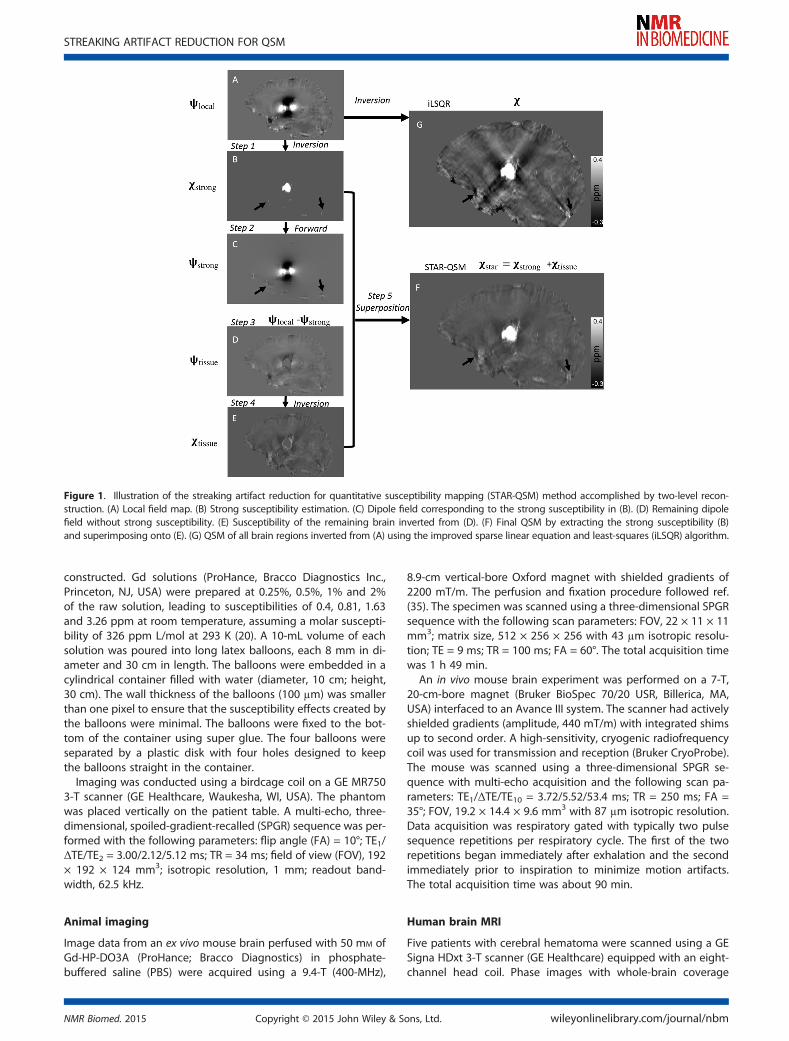
does not accommodate the potential large variations in suscep-tibility values. In Equation [3], λ determines the smoothness ofthe reconstructed susceptibility map: larger values yieldsmoother images, whereas smaller values can provide better es-timations of subtle susceptibility variations. Variation of the reg-ularization parameter allows us to control the scale of spatialfeature present in the QSM calculation. Therefore, we proposea two-level susceptibility estimation method as illustrated inFig. 1. ψlocal is the filtered tissue phase, which, in this case, is cal-culated with V-SHARP (11). In step 1, Equation [3] is solved with alarge λ, which results in an estimation of the strong susceptibilitysources (Fig. 1B). In step 2, the dipole field (Fig. 1C) correspond-ing to the strong susceptibility sources is obtained by a forwardcalculation following Equation [1]. In step 3, this strong dipolefield is subtracted from the total phase (Fig. 1D). In step 4, thesusceptibility map corresponding to the residual phase is ob-tained after inversion with a typical, small TV weighting parame-ter β (Fig. 1E). Finally, the strong susceptibility (Fig. 1B) issuperimposed onto the remaining brain susceptibility (Fig. 1E),yielding the final QSM results in Fig. 1F. We refer to this two-levelsusceptibility estimation as streaking artifact reduction for QSM(STAR-QSM) with large dynamic range.

Phantom

To evaluate the quantitative accuracy of STAR-QSM, a cylindricalphantom with a known susceptibility distribution was

H. WEI ET AL.

wileyonlinelibrary.com/journal/nbm Copyright © 2015 John Wiley & Sons, Ltd. NMR Biomed. 2015

constructed. Gd solutions (ProHance, Bracco Diagnostics Inc.,Princeton, NJ, USA) were prepared at 0.25%, 0.5%, 1% and 2%of the raw solution, leading to susceptibilities of 0.4, 0.81, 1.63and 3.26 ppm at room temperature, assuming a molar suscepti-bility of 326 ppm L/mol at 293 K (20). A 10-mL volume of eachsolution was poured into long latex balloons, each 8 mm in di-ameter and 30 cm in length. The balloons were embedded in acylindrical container filled with water (diameter, 10 cm; height,30 cm). The wall thickness of the balloons (100 μm) was smallerthan one pixel to ensure that the susceptibility effects created bythe balloons were minimal. The balloons were fixed to the bot-tom of the container using super glue. The four balloons wereseparated by a plastic disk with four holes designed to keepthe balloons straight in the container.Imaging was conducted using a birdcage coil on a GE MR750

3-T scanner (GE Healthcare, Waukesha, WI, USA). The phantomwas placed vertically on the patient table. A multi-echo, three-dimensional, spoiled-gradient-recalled (SPGR) sequence was per-formed with the following parameters: flip angle (FA) = 10°; TE1/ΔTE/TE2 = 3.00/2.12/5.12 ms; TR = 34 ms; field of view (FOV), 192× 192 × 124 mm3; isotropic resolution, 1 mm; readout band-width, 62.5 kHz.

Animal imaging

Image data from an ex vivo mouse brain perfused with 50 mM ofGd-HP-DO3A (ProHance; Bracco Diagnostics) in phosphate-buffered saline (PBS) were acquired using a 9.4-T (400-MHz),

8.9-cm vertical-bore Oxford magnet with shielded gradients of2200 mT/m. The perfusion and fixation procedure followed ref.(35). The specimen was scanned using a three-dimensional SPGRsequence with the following scan parameters: FOV, 22 × 11 × 11mm3; matrix size, 512 × 256 × 256 with 43 μm isotropic resolu-tion; TE = 9 ms; TR = 100 ms; FA = 60°. The total acquisition timewas 1 h 49 min.

An in vivo mouse brain experiment was performed on a 7-T,20-cm-bore magnet (Bruker BioSpec 70/20 USR, Billerica, MA,USA) interfaced to an Avance III system. The scanner had activelyshielded gradients (amplitude, 440 mT/m) with integrated shimsup to second order. A high-sensitivity, cryogenic radiofrequencycoil was used for transmission and reception (Bruker CryoProbe).The mouse was scanned using a three-dimensional SPGR se-quence with multi-echo acquisition and the following scan pa-rameters: TE1/ΔTE/TE10 = 3.72/5.52/53.4 ms; TR = 250 ms; FA =35°; FOV, 19.2 × 14.4 × 9.6 mm3 with 87 μm isotropic resolution.Data acquisition was respiratory gated with typically two pulsesequence repetitions per respiratory cycle. The first of the tworepetitions began immediately after exhalation and the secondimmediately prior to inspiration to minimize motion artifacts.The total acquisition time was about 90 min.

Human brain MRI

Five patients with cerebral hematoma were scanned using a GESigna HDxt 3-T scanner (GE Healthcare) equipped with an eight-channel head coil. Phase images with whole-brain coverage

Figure 1. Illustration of the streaking artifact reduction for quantitative susceptibility mapping (STAR-QSM) method accomplished by two-level recon-struction. (A) Local field map. (B) Strong susceptibility estimation. (C) Dipole field corresponding to the strong susceptibility in (B). (D) Remaining dipolefield without strong susceptibility. (E) Susceptibility of the remaining brain inverted from (D). (F) Final QSM by extracting the strong susceptibility (B)and superimposing onto (E). (G) QSM of all brain regions inverted from (A) using the improved sparse linear equation and least-squares (iLSQR) algorithm.

STREAKING ARTIFACT REDUCTION FOR QSM

NMR Biomed. 2015 Copyright © 2015 John Wiley & Sons, Ltd. wileyonlinelibrary.com/journal/nbm

were acquired using a standard flow-compensated three-dimensional SPGR sequence with the following parameters:TE1/ΔTE/TE16 = 3.16/4.85/75.9 ms; TR = 43 ms; FA = 12°; FOV,220 × 220 × 132 mm3; matrix size, 256 × 256 × 66. This protocolresulted in an isotropic in-plane resolution (0.86 × 0.86 mm2)with a slice thickness of 2 mm. The total acquisition time wasabout 12 min.

In vivo brain image data from four patients with MS were ac-quired on a GE MR750 3.0-T scanner using a three-dimensionalSPGR sequence with the following parameters: TE1/ΔTE/TE16 =3.00/4.18/65.7 ms; TR = 54 ms; FA = 12°; FOV, 220 × 220 × 132mm3; matrix size, 256 × 256 × 132; spatial resolution, 0.86 ×0.86 × 1 mm3. All experiments were approved by the local insti-tutional review boards. The total acquisition time was about 30min.

Image analysis

Human brain data were interpolated to an isotropic resolution of0.86 × 0.86 × 0.86 by zero padding in k space. The raw phase wasunwrapped using Laplacian-based phase unwrapping. The nor-malized phase ψ was calculated as:

ψ ¼ ∑ni¼1φiγμ0H0∑ni¼1TEi

[5]

where n is the number of echoes. The normalized backgroundphase was removed by V-SHARP (11,23). The magnitude imagewas used to extract the brain tissue. The magnetic susceptibilitywas determined using STAR-QSM and compared with iLSQR. The

iterative solver was terminated when the relative residual normwas less than 0.01 (maximum of 200 iterations). All of the pro-grams were written using Matlab R2011b (Mathworks, Natick,MA, USA).

RESULTS

Algorithm parameter optimization

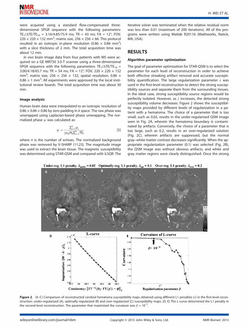
The goal of parameter optimization for STAR-QSM is to select theparameter for each level of reconstruction in order to achieveboth effective streaking artifact removal and accurate suscepti-bility quantification. The large regularization parameter λ wasused in the first-level reconstruction to detect the strong suscep-tibility sources and separate them from the surrounding tissues.In the ideal case, strong susceptibility source regions would beperfectly isolated. However, as λ increases, the detected strongsusceptibility volume decreases. Figure 2 shows the susceptibil-ity maps provided by different levels of regularization in a pa-tient with a hematoma. The choice of a parameter that is toosmall, such as 0.02, results in the under-regularized QSM imageseen in Fig. 2A, wherein the hematoma boundary is contami-nated by artifacts. Conversely, the choice of a parameter that istoo large, such as 0.2, results in an over-regularized solution(Fig. 2C), wherein artifacts are suppressed, but the normalgray–white matter contrast decreases significantly. When the ap-propriate regularization parameter (0.1) was selected (Fig. 2B),the QSM image was without obvious artifacts, and white andgray matter regions were clearly distinguished. Once the strong

Figure 2. (A–C) Comparison of reconstructed cerebral hematoma susceptibility maps obtained using different L1 penalties (λ) in the first-level recon-struction: under-regularized (A), optimally regularized (B) and over-regularized (C) susceptibility maps. (D, E) The L-curve determined the L1 penalty inthe second-level reconstruction. The parameter that maximized the curvature was β = 10–5.

H. WEI ET AL.

wileyonlinelibrary.com/journal/nbm Copyright © 2015 John Wiley & Sons, Ltd. NMR Biomed. 2015

susceptibility source was detected from the first-level recon-struction, the corresponding dipole field was then removed fromthe remaining brain regions. The second-level reconstructionthen calculated the susceptibility of the remaining brain regionswithout the strong susceptibility source. This step fully invertedthe remaining dipole field as shown by step 4 in Fig. 1. The opti-mization for the relatively small regularization parameter can bedetermined by maximizing the curvature of the L-curve. Eachpoint on the L-curve was reconstructed using 200 iterations ofthe L1 regularization. In order to distinguish it from the first-levelparameter (λ), the second-level regularization parameter was re-ferred to as β. The corner of the L-curve is not obvious (Fig. 2D);however, the optimum regularization parameter can be deter-mined from the curvature with β < 10–5 (Fig. 2E). Therefore,10–5 was selected as the optimal parameter in the second-stepreconstruction. This parameter was fixed for the QSM reconstruc-tion of the tissues with narrow susceptibility range. Therefore, forSTAR-QSM, the regularization parameter λ in the first-level recon-struction was the only user-defined parameter.

Gd phantom

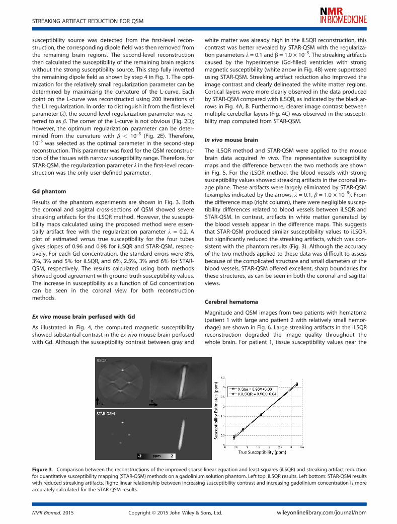
Results of the phantom experiments are shown in Fig. 3. Boththe coronal and sagittal cross-sections of QSM showed severestreaking artifacts for the iLSQR method. However, the suscepti-bility maps calculated using the proposed method were essen-tially artifact free with the regularization parameter λ = 0.2. Aplot of estimated versus true susceptibility for the four tubesgives slopes of 0.96 and 0.98 for iLSQR and STAR-QSM, respec-tively. For each Gd concentration, the standard errors were 8%,3%, 3% and 5% for iLSQR, and 6%, 2.5%, 3% and 6% for STAR-QSM, respectively. The results calculated using both methodsshowed good agreement with ground truth susceptibility values.The increase in susceptibility as a function of Gd concentrationcan be seen in the coronal view for both reconstructionmethods.

Ex vivo mouse brain perfused with Gd

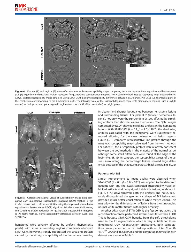
As illustrated in Fig. 4, the computed magnetic susceptibilityshowed substantial contrast in the ex vivo mouse brain perfusedwith Gd. Although the susceptibility contrast between gray and

white matter was already high in the iLSQR reconstruction, thiscontrast was better revealed by STAR-QSM with the regulariza-tion parameters λ = 0.1 and β = 1.0 × 10–5. The streaking artifactscaused by the hyperintense (Gd-filled) ventricles with strongmagnetic susceptibility (white arrow in Fig. 4B) were suppressedusing STAR-QSM. Streaking artifact reduction also improved theimage contrast and clearly delineated the white matter regions.Cortical layers were more clearly observed in the data producedby STAR-QSM compared with iLSQR, as indicated by the black ar-rows in Fig. 4A, B. Furthermore, clearer image contrast betweenmultiple cerebellar layers (Fig. 4C) was observed in the suscepti-bility map computed from STAR-QSM.

In vivo mouse brain

The iLSQR method and STAR-QSM were applied to the mousebrain data acquired in vivo. The representative susceptibilitymaps and the difference between the two methods are shownin Fig. 5. For the iLSQR method, the blood vessels with strongsusceptibility values showed streaking artifacts in the coronal im-age plane. These artifacts were largely eliminated by STAR-QSM(examples indicated by the arrows, λ = 0.1, β = 1.0 × 10–5). Fromthe difference map (right column), there were negligible suscep-tibility differences related to blood vessels between iLSQR andSTAR-QSM. In contrast, artifacts in white matter generated bythe blood vessels appear in the difference maps. This suggeststhat STAR-QSM produced similar susceptibility values to iLSQR,but significantly reduced the streaking artifacts, which was con-sistent with the phantom results (Fig. 3). Although the accuracyof the two methods applied to these data was difficult to assessbecause of the complicated structure and small diameters of theblood vessels, STAR-QSM offered excellent, sharp boundaries forthese structures, as can be seen in both the coronal and sagittalviews.

Cerebral hematoma

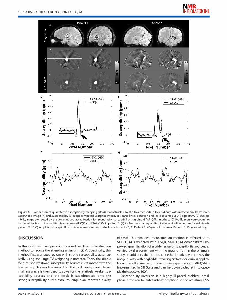
Magnitude and QSM images from two patients with hematoma(patient 1 with large and patient 2 with relatively small hemor-rhage) are shown in Fig. 6. Large streaking artifacts in the iLSQRreconstruction degraded the image quality throughout thewhole brain. For patient 1, tissue susceptibility values near the

Figure 3. Comparison between the reconstructions of the improved sparse linear equation and least-squares (iLSQR) and streaking artifact reductionfor quantitative susceptibility mapping (STAR-QSM) methods on a gadolinium solution phantom. Left top: iLSQR results. Left bottom: STAR-QSM resultswith reduced streaking artifacts. Right: linear relationship between increasing susceptibility contrast and increasing gadolinium concentration is moreaccurately calculated for the STAR-QSM results.

STREAKING ARTIFACT REDUCTION FOR QSM

NMR Biomed. 2015 Copyright © 2015 John Wiley & Sons, Ltd. wileyonlinelibrary.com/journal/nbm

hematoma were severely affected by artifacts (hypointensepixels), with some surrounding regions completely obscured.STAR-QSM, however, strongly suppressed the streaking artifactscaused by the strong susceptibility of the hematoma, resulting

in cleaner and sharper boundaries between hematoma lesionsand surrounding tissues. For patient 2 (smaller hematoma le-sions), not only were the surrounding tissues affected by streak-ing artifacts, but also the lesions themselves. The QSM imagescomputed by iLSQR showed streaking artifacts in the hematomalesions. With STAR-QSM (λ = 0.1, β = 1.0 × 10–5), the shadowingartifacts associated with the hematoma were successfully re-moved, allowing for the clear delineation of lesion regions.Figure 6D–F compares representative line profiles through themagnetic susceptibility maps calculated from the two methods.For patient 1, the susceptibility profiles were relatively consistentbetween the two methods in the majority of the normal tissue,although some small differences were found at the edge of thebrain (Fig. 6F, G). In contrast, the susceptibility values of the tis-sues surrounding the hemorrhagic lesions showed large differ-ences because of the shadowing artifacts (black arrows, Fig. 6D, E).

Patients with MS

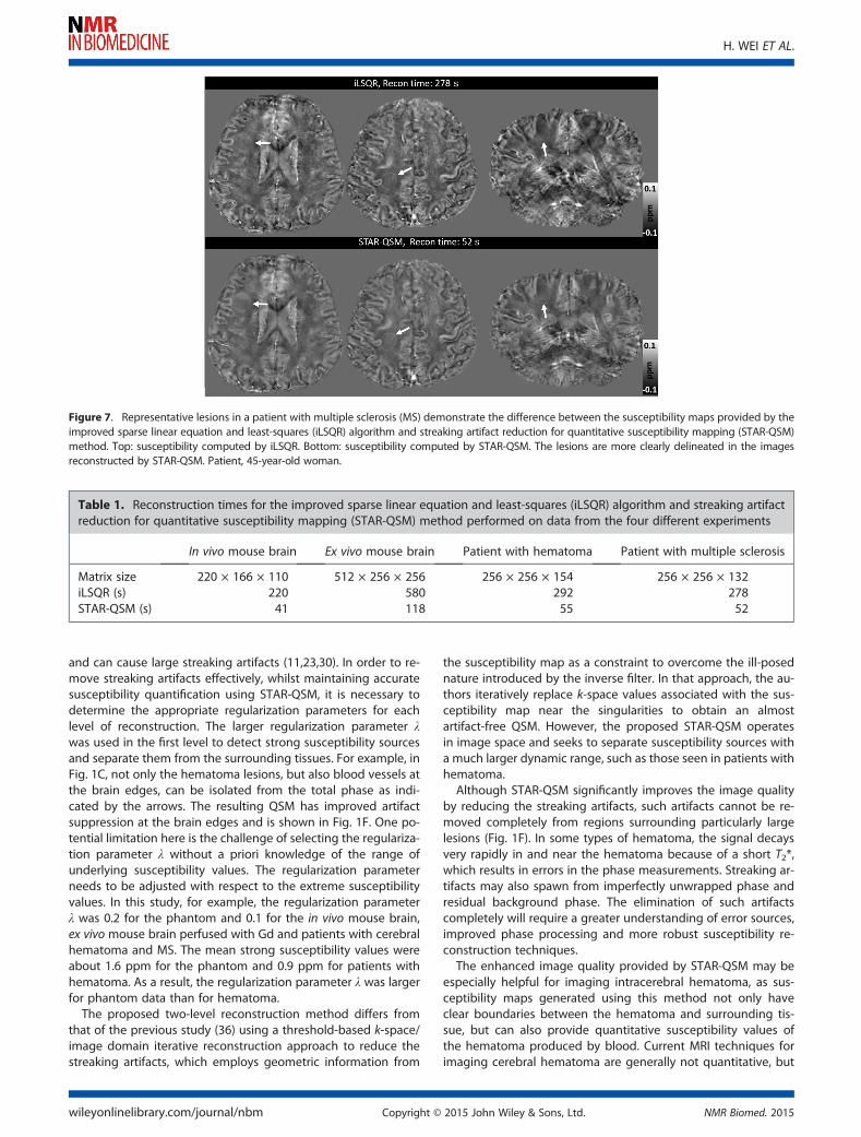
Similar improvements to image quality were observed whenSTAR-QSM (λ = 0.1, β = 1.0 × 10–5) was applied to the data frompatients with MS. The iLSQR-computed susceptibility maps ex-hibited artifacts and noisy signal inside the lesions, as shown inFig. 7. STAR-QSM removed both the artifacts and noise, accu-rately distinguished the geometrical shape of MS lesions andprovided much better visualization of white matter lesions. Thismay allow for the differentiation of lesions from the surroundingnormal white matter tissues with higher accuracy.Another advantage of STAR-QSM is the fast computation; this

reconstruction can be performed several times faster than iLSQR.This is because STAR-QSM benefits from the soft thresholdingused in the L1 regularization which is very suitable for three-dimensional QSM reconstruction applications. Both computa-tions were performed on a desktop with an Intel Core i7-4770TM CPU and 16 GB RAM, and the computation times for eachdataset are shown in Table 1.

Figure 4. Coronal (A) and sagittal (B) views of ex vivo mouse brain susceptibility maps comparing improved sparse linear equation and least-squares(iLSQR) algorithm and streaking artifact reduction for quantitative susceptibility mapping (STAR-QSM) method. Top: susceptibility maps obtained usingiLSQR. Middle: susceptibility maps obtained using STAR-QSM. Bottom: susceptibility difference between iLSQR and STAR-QSM. (C) Zoomed regions ofthe cerebellum corresponding to the black boxes in (B). The intensity scale of the susceptibility maps represents diamagnetic regions (such as whitematter) as dark pixels and paramagnetic regions (such as the Gd-filled ventricles) as bright pixels.

Figure 5. Coronal and sagittal views of susceptibility image data com-paring each quantitative susceptibility mapping (QSM) method in thein vivo mouse brain. Left: susceptibility using the improved sparse linearequation and least-squares (iLSQR) algorithm. Middle: susceptibility usingthe streaking artifact reduction for quantitative susceptibility mapping(STAR-QSM) method. Right: susceptibility difference between iLSQR andSTAR-QSM.

H. WEI ET AL.

wileyonlinelibrary.com/journal/nbm Copyright © 2015 John Wiley & Sons, Ltd. NMR Biomed. 2015

DISCUSSION

In this study, we have presented a novel two-level reconstructionmethod to reduce the streaking artifacts in QSM. Specifically, thismethod first estimates regions with strong susceptibility automat-ically using the large TV weighting parameter. Then, the dipolefield caused by strong susceptibility sources is estimated with theforward equation and removed from the total tissue phase. The re-maining phase is then used to solve for the relatively weaker sus-ceptibility sources and the result is superimposed onto thestrong susceptibility distribution, resulting in an improved quality

of QSM. This two-level reconstruction method is referred to asSTAR-QSM. Compared with iLSQR, STAR-QSM demonstrates im-proved quantification of a wide range of susceptibility sources, asverified by the agreement with the ground truth in the phantomstudy. In addition, the proposed method markedly improves theimage quality with negligible streaking artifacts for various applica-tions in small animal and human brain experiments. STAR-QSM isimplemented in STI Suite and can be downloaded at http://peo-ple.duke.edu/~cl160/.

Susceptibility inversion is a highly ill-posed problem. Smallphase error can be substantially amplified in the resulting QSM

Figure 6. Comparison of quantitative susceptibility mapping (QSM) reconstructed by the two methods in two patients with intracerebral hematoma.Magnitude image (A) and susceptibility (B) maps computed using the improved sparse linear equation and least-squares (iLSQR) algorithm. (C) Suscep-tibility maps computed by the streaking artifact reduction for quantitative susceptibility mapping (STAR-QSM) method. (D) Profile plots correspondingto the white line on the sagittal view between iLSQR and STAR-QSM in patient 1. (E) Profile plots corresponding to the white line on the coronal view inpatient 2. (F, G) Amplified susceptibility profiles corresponding to the black boxes in D, E. Patient 1, 46-year-old woman. Patient 2, 15-year-old boy.

STREAKING ARTIFACT REDUCTION FOR QSM

NMR Biomed. 2015 Copyright © 2015 John Wiley & Sons, Ltd. wileyonlinelibrary.com/journal/nbm

and can cause large streaking artifacts (11,23,30). In order to re-move streaking artifacts effectively, whilst maintaining accuratesusceptibility quantification using STAR-QSM, it is necessary todetermine the appropriate regularization parameters for eachlevel of reconstruction. The larger regularization parameter λwas used in the first level to detect strong susceptibility sourcesand separate them from the surrounding tissues. For example, inFig. 1C, not only the hematoma lesions, but also blood vessels atthe brain edges, can be isolated from the total phase as indi-cated by the arrows. The resulting QSM has improved artifactsuppression at the brain edges and is shown in Fig. 1F. One po-tential limitation here is the challenge of selecting the regulariza-tion parameter λ without a priori knowledge of the range ofunderlying susceptibility values. The regularization parameterneeds to be adjusted with respect to the extreme susceptibilityvalues. In this study, for example, the regularization parameterλ was 0.2 for the phantom and 0.1 for the in vivo mouse brain,ex vivo mouse brain perfused with Gd and patients with cerebralhematoma and MS. The mean strong susceptibility values wereabout 1.6 ppm for the phantom and 0.9 ppm for patients withhematoma. As a result, the regularization parameter λ was largerfor phantom data than for hematoma.

The proposed two-level reconstruction method differs fromthat of the previous study (36) using a threshold-based k-space/image domain iterative reconstruction approach to reduce thestreaking artifacts, which employs geometric information from

the susceptibility map as a constraint to overcome the ill-posednature introduced by the inverse filter. In that approach, the au-thors iteratively replace k-space values associated with the sus-ceptibility map near the singularities to obtain an almostartifact-free QSM. However, the proposed STAR-QSM operatesin image space and seeks to separate susceptibility sources witha much larger dynamic range, such as those seen in patients withhematoma.Although STAR-QSM significantly improves the image quality

by reducing the streaking artifacts, such artifacts cannot be re-moved completely from regions surrounding particularly largelesions (Fig. 1F). In some types of hematoma, the signal decaysvery rapidly in and near the hematoma because of a short T2*,which results in errors in the phase measurements. Streaking ar-tifacts may also spawn from imperfectly unwrapped phase andresidual background phase. The elimination of such artifactscompletely will require a greater understanding of error sources,improved phase processing and more robust susceptibility re-construction techniques.The enhanced image quality provided by STAR-QSM may be

especially helpful for imaging intracerebral hematoma, as sus-ceptibility maps generated using this method not only haveclear boundaries between the hematoma and surrounding tis-sue, but can also provide quantitative susceptibility values ofthe hematoma produced by blood. Current MRI techniques forimaging cerebral hematoma are generally not quantitative, but

Figure 7. Representative lesions in a patient with multiple sclerosis (MS) demonstrate the difference between the susceptibility maps provided by theimproved sparse linear equation and least-squares (iLSQR) algorithm and streaking artifact reduction for quantitative susceptibility mapping (STAR-QSM)method. Top: susceptibility computed by iLSQR. Bottom: susceptibility computed by STAR-QSM. The lesions are more clearly delineated in the imagesreconstructed by STAR-QSM. Patient, 45-year-old woman.

Table 1. Reconstruction times for the improved sparse linear equation and least-squares (iLSQR) algorithm and streaking artifactreduction for quantitative susceptibility mapping (STAR-QSM) method performed on data from the four different experiments

In vivo mouse brain Ex vivo mouse brain Patient with hematoma Patient with multiple sclerosis

Matrix size 220 × 166 × 110 512 × 256 × 256 256 × 256 × 154 256 × 256 × 132iLSQR (s) 220 580 292 278STAR-QSM (s) 41 118 55 52

H. WEI ET AL.

wileyonlinelibrary.com/journal/nbm Copyright © 2015 John Wiley & Sons, Ltd. NMR Biomed. 2015

the treatment of hematoma may require volume measurement(37,38). In particular, QSM, with reduced streaking artifactsaround the hematoma, may allow a more accurate quantificationof susceptibility values produced by the blood, permitting po-tential staging of the bleed. The application of standard QSMmethods to hematoma volume measurement and susceptibilityquantification is limited in that susceptibility values in the centralhematoma can be affected by the complicated boundary shape(9). Similar susceptibility values were found inside the lesions be-tween iLSQR and STAR-QSM performed on patient 1, in whichthe hematoma region was round. However, the susceptibilityvalues from iLSQR and STAR-QSM differed substantially insidethe hematoma in patient 2, probably as a result of the compli-cated lesion geometry and the streaking artifacts in iLSQR. Theapparent higher contrast of the susceptibility profile outsidethe hematoma lesions computed by iLSQR is made up of twosources. One is that the streaking artifacts are created not onlyby the hematoma itself, but also by the strong susceptibilitysources (i.e. veins) near the brain edges (black arrows in Fig. 1G).The other is noise amplification, a major issue in the ill-posed in-verse calculation, which manifests itself as streaking artifacts andquantification errors in QSM. However, STAR-QSM incorporates aTV term as a regularizer in Equation [3], which can effectivelysuppress noise amplification (11). Using the two-level QSM re-construction, the streaking artifacts were significantly reduced.Although the phantom experiment illustrated the accuracy ofSTAR-QSM compared with the ground truth, it remains to be de-termined whether the TV term reduces normal tissue contrasteven with the small regularization parameter chosen (β = 1.0 ×10–5). The representative line profiles (Fig. 6D, E) show the re-duced susceptibility errors around the hematoma when usingthe proposed method. It is acknowledged that the actual accu-racy of each method is difficult to assess as no ‘ground truth’ in-formation is available. However, STAR-QSM enables the cleardelineation of the hematoma boundaries with less artifact con-tamination. Such evidence confirms that the susceptibility quan-tification provided by our new two-level reconstruction methodis satisfactorily accurate.The enhanced image quality with lower noise level provided

by STAR-QSM in patients with MS may be especially helpful forthe imaging of MS. Although there are no obvious large suscep-tibility sources within the MS lesions themselves, veins near thebrain edges generally appear highly paramagnetic. Such strongsources will create numerous streaking artifacts throughout thewhole brain. As a result, not only the white matter MS lesions,but also the normal brain tissue, will be degraded by such arti-facts (shown by the black arrows in Fig. 1B, C, G, F). STAR-QSMcan estimate the strong susceptibility sources and remove theresulting streaking artifacts. This artifact reduction allows for aclearer visualization of MS lesions and normal brain tissues. Fur-thermore, the incorporation of the TV term as a regularizationterm in the core function of STAR-QSM in Equation [3] alleviatesthe amplified noise propagation of the ill-posed inverse calcula-tion and improves the quality of the susceptibility map. Specifi-cally, this regularization yields clearer MS lesion boundaries andlower noise levels compared with iLSQR.

CONCLUSION

In this article, we have proposed a new QSM reconstructionmethod, STAR-QSM, to reduce the streaking artifacts caused by

strong suceptibility sources. The dipole fields of the strong sus-ceptibility sources were determined and then separated fromthe total phase to remove the streaking artifacts. Data from aphantom, in vivo and ex vivo mouse brain and patients with ce-rebral hematoma or MS showed significantly reduced streakingartifacts with improved image quality. The enhancement is help-ful for various applications, in particular, the imaging of humanintracerebral hematoma.

Acknowledgements

This study was supported in part by the National Institutes ofHealth through grants NIBIB P41EB015897, NIBIB T32EB001040,NIMH R01MH096979, NINDS R01NS079653, NIMH R24MH106096and NHLBI R21HL122759, and by the National Multiple SclerosisSociety through grant RG4723.

REFERENCES1. Abduljalil AM, Schmalbrock P, Novak V, Chakeres DW. Enhanced gray

and white matter contrast of phase susceptibility-weighted imagesin ultra-high-field magnetic resonance imaging. J. Magn. Reson. Im-aging, 2003; 18: 284–290.

2. Haacke EM, Xu Y, Cheng Y-CN, Reichenbach JR. Susceptibilityweighted imaging (SWI). Magn. Reson. Med. 2004; 52: 612–618.

3. Wycliffe ND, Choe J, Holshouser B, Oyoyo UE, Haacke EM, Kido DK.Reliability in detection of hemorrhage in acute stroke by a newthree-dimensional gradient recalled echo susceptibility-weightedimaging technique compared to computed tomography: a retro-spective study. J. Magn. Reson. Imaging, 2004; 20: 372–377.

4. Rauscher A, Sedlacik J, Barth M, Mentzel HJ, Reichenbach JR. Mag-netic susceptibility-weighted MR phase imaging of the human brain.Am. J. Neuroradiol. 2005; 26: 736–742.

5. Duyn JH, van Gelderen P, Li T-Q, de Zwart JA, Koretsky AP, FukunagaM. High-field MRI of brain cortical substructure based on signalphase. Proc. Natl. Acad. Sci. U. S. A., 2007; 104: 11 796–11 801.

6. Shmueli K, de Zwart JA, van Gelderen P, Li T-Q, Dodd SJ, Duyn JH.Magnetic susceptibility mapping of brain tissue in vivo using MRIphase data. Magn. Reson. Med. 2009; 62: 1510–1522.

7. Fukunaga M, Li T-Q, van Gelderen P, Zwart JA, Shmueli K, Yao B, Lee J,Maric D, AronovaMA, ZhangG, Leapman RD, Schenck JF, Merkle H, GuynJH. Layer-specific variation of iron content in cerebral cortex as a sourceof MRI contrast. Proc. Natl. Acad. Sci. U. S. A., 2010; 107: 3834–3839.

8. Lee J, Shmueli K, Fukunaga M, van Gelderen P, Merkle H, Silva AC,Duyn JH. Sensitivity of MRI resonance frequency to the orientationof brain tissue microstructure. Proc. Natl. Acad. Sci. U. S. A., 2010;107: 5130–5135.

9. Li N. Magnetic susceptibility quantification for arbitrarily shaped ob-jects in inhomogeneous fields. Magn. Reson. Med. 2001; 46: 907–916.

10. Li W, Wu B, Liu C. Quantitative susceptibility mapping of humanbrain reflects spatial variation in tissue composition. Neuroimage,2011; 55: 1645–1656.

11. Wu B, Li W, Guidon A, Liu C. Whole brain susceptibility mappingusing compressed sensing. Magn. Reson. Med. 2012; 67: 137–147.

12. De Rochefort L, Liu T, Kressler B, Liu J, Spincemaille P, Lebon V, Wu J,Wang Y. Quantitative susceptibility map reconstruction from MRphase data using bayesian regularization: validation and applicationto brain imaging. Magn. Reson. Med. 2010; 63: 194–206.

13. Wharton S, Schäfer A, Bowtell R. Susceptibility mapping in the hu-man brain using threshold-based k-space division. Magn. Reson.Med. 2010; 63: 1292–1304.

14. Liu T, Wisnieff C, Lou M, Chen W, Spincemaille P, Wang Y. Nonlinearformulation of the magnetic field to source relationship for robustquantitative susceptibility mapping. Magn. Reson. Med. 2013; 69:467–476.

15. Schweser F, Deistung A, Sommer K, Reichenbach JR. Toward onlinereconstruction of quantitative susceptibility maps: superfast dipoleinversion. Magn. Reson. Med. 2013; 69: 1582–1594.

16. Sun H, Wilman AH. Background field removal using spherical meanvalue filtering and Tikhonov regularization. Magn. Reson. Med.2014; 71: 1151–1157.

STREAKING ARTIFACT REDUCTION FOR QSM

NMR Biomed. 2015 Copyright © 2015 John Wiley & Sons, Ltd. wileyonlinelibrary.com/journal/nbm

17. Chen W, Zhu W, Kovanlikaya I, Kovanlikaya A, Liu T, Wang S, SalustriC, Wang Y. Intracranial calcifications and hemorrhages: characteriza-tion with quantitative susceptibility mapping. Radiology, 2014; 270:496–505.

18. Bonekamp D, Barker PB, Leigh R, van Zijl PCM, Li X. Susceptibility-based analysis of dynamic gadolinium bolus perfusion MRI. Magn.Reson. Med. 2014; 554: 544–554.

19. Balla DZ, Sanchez-Panchuelo RM, Wharton SJ, Hagberg GE, SchefflerK, Francis ST, Bowtell R. Functional quantitative susceptibility map-ping (fQSM). Neuroimage, 2014; 100: 112–124.

20. De Rochefort L, Brown R, Prince MR, Wang Y. Quantitative MR sus-ceptibility mapping using piece-wise constant regularized inversionof the magnetic field. Magn. Reson. Med. 2008; 60: 1003–1009.

21. Wen Y, Wang Y, Liu T. Enhancing k-space quantitative susceptibilitymapping by enforcing consistency on the cone data (CCD) withstructural priors. Magn. Reson. Med. 2015; Epub ahead of print.

22. Schweser F, Sommer K, Deistung A, Reichenbach JR. Quantitativesusceptibility mapping for investigating subtle susceptibility varia-tions in the human brain. Neuroimage, 2012; 62: 2083–2100.

23. Li W, Wang N, Yu F, Han H, Cao W, Romero R, Tantiwongkosi B, DuongTQ, Liu C. A method for estimating and removing streaking artifacts inquantitative susceptibility mapping. Neuroimage, 2015; 108: 111–122.

24. Liu T, Spincemaille P, De Rochefort L, Kressler B, Wang Y. Calculationof susceptibility through multiple orientation sampling (COSMOS): amethod for conditioning the inverse problem from measured mag-netic field map to susceptibility source image in MRI. Magn. Reson.Med. 2009; 61: 196–204.

25. Bilgic B, Pfefferbaum A, Rohlfing T, Sullivan EV, Adalsteinsson E. MRIestimates of brain iron concentration in normal aging using quanti-tative susceptibility mapping. Neuroimage, 2012; 59: 2625–2635.

26. Langkammer C, Bredies K, Poser BA, Barth M, Reishofer G, Fan AP,Bilgic B, Fazekas F, Mainero C, Ropele S. Fast quantitative susceptibil-ity mapping using 3D EPI and total generalized variation.Neuroimage, 2015; 111:622–630.

27. Lustig M, Donoho D, Pauly JM. Sparse MRI: the application of com-pressed sensing for rapid MR imaging. Magn. Reson. Med. 2007;58: 1182–1195.

28. Liang D, Wang H, Chang Y, Ying L. Sensitivity encoding reconstruc-tion with nonlocal total variation regularization. Magn. Reson. Med.2011; 65: 1384–1392.

29. Bilgic B, Fan AP, Polimeni JR, Cauley SF, Bianciardi M, Adalsteinsson E,Wald LL, Setsompop K. Fast quantitative susceptibility mapping with

L1-regularization and automatic parameter selection. Magn. Reson.Med. 2013; 1459: 1444–1459.

30. Wei H, Li W, Wang N, Liu C. Streaking artifact reduction for QSM. 3rdInternational Workshop on MRI Phase Contrast Quantitative Suscep-tibility Mapping, Durham, NC, USA, October 6–8, 2014.

31. Salomir R, De Senneville BD, Moonen CTW. A fast calculation methodfor magnetic field inhomogeneity due to an arbitrary distribution ofbulk susceptibility. Concepts Magn. Reson. Part B: Magn. Reson. Eng.2003; 19: 26–34.

32. Marques JP, Bowtell R. Application of a Fourier-based method forrapid calculation of field inhomogeneity due to spatial variation ofmagnetic susceptibility. Concepts Magn. Reson. Part B: Magn. Reson.Eng. 2005; 25: 65–78.

33. Wharton S, Bowtell R. Whole-brain susceptibility mapping at highfield: a comparison of multiple- and single-orientation methods.Neuroimage, 2010; 53: 515–525.

34. Wright SJ, Nowak RD, Figueiredo MAT. Sparse reconstruction by sepa-rable approximation. IEEE Trans. Signal Process. 2009; 57: 2479–2493.

35. Dibb R, Li W, Cofer G, Liu C. Microstructural origins of gadolinium-enhanced susceptibility contrast and anisotropy. Magn. Reson.Med. 2014; 1711: 1702–1711.

36. Tang J, Liu S, Neelavalli J, Cheng YCN, Buch S, Haacke EM. Improvingsusceptibility mapping using a threshold-based K-space/image do-main iterative reconstruction approach. Magn. Reson. Med. 2013;69: 1396–1407.

37. Christoforidis GA, Slivka A, Mohammad Y, Karakasis C, Avutu B, YangM. Size matters: hemorrhage volume as an objective measure to de-fine significant intracranial hemorrhage associated with thromboly-sis. Stroke, 2007; 38: 1799–1804.

38. Zimmerman RD, Maldjian JA, Brun NC, Horvath B, Skolnick BE. Radio-logic estimation of hematoma volume in intracerebral hemorrhagetrial by CT scan. Am. J. Neuroradiol. 2006; 27: 666–670.

SUPPORTING INFORMATIONSupporting information may be found in the online version ofthis article at the publisher’s web site.

H. WEI ET AL.

wileyonlinelibrary.com/journal/nbm Copyright © 2015 John Wiley & Sons, Ltd. NMR Biomed. 2015