Strategic noise mapping with GIS for the Universitat Jaume ...

i

Strategic noise mapping with GIS for the Universitat Jaume I Smart Campus: Best Methodology Practices

Sarah Eason

ii

Strategic noise mapping with GIS for the Universitat Jaume I Smart Campus: Best Methodology Practices

Sarah Eason

iii

Strategic noise mapping with GIS for the Universitat Jaume I Smart Campus: Best methodology practices

by Sarah Eason

[email protected] Institute of New Imaging Systems,

Universitat Jaume I, Castellon, Spain

Dissertation supervised by

Michael Gould, PhD Global Education Manager, ESRI

Professor of Information Systems, Institute of New Imaging Systems, Universitat Jaume I,

Castellon, Spain

Dissertation co-supervised by

Joaquin Huerta, PhD Professor, Institute of New Imaging Systems,

Universitat Jaume I, Castellon, Spain

Marco Pinho, PhD Instituto Superior de Estatica e Gestau de Informacao

Universidade NOVA de Lisboa Lisbon, Portugal

March 1, 2013

iv

ACKNOWLEDGEMENTS

I would like to thank Dr. Michael Gould for supervising my thesis and Dr. Joaquin Huerta and Dr. Marco Painho for co-supervising. I am privileged to have participated in the Master of Science in Geospatial Technologies. I thank the Erasmus Mundus Association, the Institute for New Imaging Technologies (INIT), Universitat Jaume I (UJI),Castellon, Spain, the Institute for Geoinformatics (IFGI), University of Munster, Germany and the Institute Superior of Statistics and Information (ISEGI), Lisbon, Portugal for providing this wonderful opportunity and all the rich experiences I have had during my time in Europe.

I would like to thank Dr. Jorge Mateu for his guidance with the statistical methodology used in this research, and Andres Munoz for his guidance with ArcGIS Modelbuilder and other GIS issues.

I also thank Luis Rodriguez a for developing the Noise Battle application and providing assistance with it and other related elements throughout my research. He was always willing and able to provide support in the programming area. I am grateful to Ana Sanchis Huerta for providing the initial idea for this thesis topic. I thank my fellow classmates for their friendship and camaraderie.

I would also like to thank ReMa Medio Ambiente, S.L. for sharing their data to make my research possible, and especially to Ricardo Blasco Troncho, Joaquin Gargallo Saura, with whom I conducted my fieldwork.

I extend my gratitude to sound engineer Bill Stevens in Texas, who kindly provided me with acoustic theory textbooks to which I would not have otherwise had access, and which made my research possible.

I would also like to thank my parents, Richard and Lynn Eason, for their constant support, emotionally, mentally, morally, financially and physically. They cheered me on and were willing at all hours of the night to review my work and discuss and revise its progress all along the way. My father was invaluable in his ability to coach me into an understanding of acoustic principles.

Finally, I want to thank my younger sister, Kathleen Eason, whose graduation from Bard College in New York prompted me to go back to school in the first place. She has been a shining light of inspiration and my best friend through it all.

v

Strategic noise mapping with GIS for the Universitat Jaume I Smart Campus: Best methodology practices

ABSTRACT

Noise is a type of pollution often overlooked in conversations about pollution, which usually center on air, water and waste management. However, it has not been missed by decision makers in the European Union (EU). There are laws to keep noise levels down, and schools are a target specifically mentioned in the European Environmental Noise Directive (END). Strategic noise mapping can identify problem areas and help evaluate situations. This thesis project explores and compares various approaches in an attempt to offer useful information to the noise mapping field based on the results of the analysis. The measurements used commonly in studies are taken by professionals using professional equipment. Either teams physically enter the environment to manually take measurements or they collect data wirelessly from fixed sensors. Both of these methods are expensive due to the manpower or equipment. In addition, these methods are limited in the number of measurements in space and time that they can represent. One option is to use citizens with smart phones to record noise measurements. Involving the public to gather information is commonly called crowdsourcing, Volunteered Geographic Information (VGI) or Public Participatory GIS (PPGIS). Three applications for Android smart phones were tested and compared to a certified, calibrated professional sound level meter. Also, mapping noise by taking sample noise measurements without also mapping noise sources may not provide the full picture. The second objective of this thesis was to apply sound attenuation and combination rules in ArcGIS to create a noise source map and compare the results to the common spatial interpolation methods. The comparisons of smart phone measurements with the professional sound level measurements revealed that they are not comparable quality. Each ANOVA and t-Test revealed statistically significant differences. This is mostly attributed to the phone’s hardware, which varies between mobile device models and versions. The geostatistical interpolation tools delivered noise maps which had similar accuracy rates for predicting measurement points according to the cross validation methods used. The best (most accurate) prediction model was indeed the kriging method. The author successfully applied sound attenuation equations to create a multiple noise source propagation and combination interpolation toolset in ArcGIS. This can be used for an infinite number of noise sources. The fit of the actual measurement points in the noise source attenuation noise map was very similar although slightly higher than that of to the geostatistical methods

KEYWORDS

ArcGIS, Crowdsourcing, GIS, European Noise Directive, Interpolation, Noise mapping, Noise pollution, PPGIS, Smart Campus, Smart Phone, Spatial analysis, VGI

vi

ACRONYMS

2D two-dimensional

ANOVA Analysis of Variance

ArcGIS Trademark name of ESRI GIS software

CESVA CESVA instruments, S.L. (private company)

dB decibel

dB(A) A-weighted decibel

den day-evening-night

END European Noise Directive

ESRI Environmental Systems Research Institute

EU European Union

GIS Geographic Information Systems or Science

GPS Global Positioning System

IDW Inverse Distance Weighted

LeqT Mean decibel level for five minute period

PPGIS public participatory GIS

RBF Radial Based Function

ReMa ReMa Medio Ambiente, S.L. (private company)

UJI Universitat Jaume I

VGI volunteered geographic information

1

1. Introduction

1.1 Rationale The Universitat Jaume I (UJI) in Castellon, Spain is in the process of becoming a Smart Campus. New technologies are being used to bring the UJI to the forefront of sustainability. With a view to improve resource management, alternative energies are being explored and conservation methods investigated. Masters students from Madrid and the Erasmus Mundus visiting scholar have joined with the team at UJI to start the creation of a two-dimensional (2D) campus map using the Environmental Systems Research Institute (ESRI) Campus Basemap Template. This project has a wide scope of opportunities to use the basemap and the tools of Geographic Information Systems (GIS). Topics range from energy consumption to facilities management to green building and sustainability. Crowdsourcing is increasing in popularity as a new way to collect data from the public, including health and allergy information, behavior monitoring and incident and problem reporting services and maintenance requests. Mobile applications for smart phones such as place finders and navigation routing for both vehicles and pedestrians can be integrated with the campus basemap. Another interesting and important application is pollution control. Noise is a type of pollution often overlooked in conversations about pollution, which usually center on air, water and waste management. However, it has not been missed by decision makers in the European Union (EU). There are laws to keep noise levels down, and schools are a target specifically mentioned in the European Environmental Noise Directive (END). Strategic noise mapping can identify problem areas and help evaluate situations. Garcia Marti et al. suggest a few approaches to noise mapping. One is to apply “physical noise propagation laws to well-known noise sources,” another is to interpolate data from a “network of sensor devices,” and a third is to build a database from data collected through the “direct participation of citizenship” (Garcia Marti 2012). This thesis project aims to explore and compare these approaches and offer useful information to the noise mapping field based on the results of the analysis.

1.2 Background In 2002, the EU created the END to address noise which has adverse effects on humans. The goals are “preventing and reducing environmental noise where necessary and particularly where exposure levels can induce harmful effects on human health and to preserving environmental noise quality where it is good.” The primary actions which are required by this directive concern monitoring the problem and informing the public, while the secondary actions to be taken as a result of the information gained are left to the judgment of the local authorities. In order to monitor the problem, measurements must be collected and noise maps must be made which represent these measurements for both day-evening-nighttime (den) and nighttime. “The selected common noise indicators are L den, to assess annoyance, and L night, to assess sleep disturbance” (Directive 2002). The strategy here is to capture measurements in areas of interest to provide useful information about the noise levels in those areas. Noises which are subject to this directive are limited to those made by automobiles, trains, aircraft and outdoor machinery. Noise generated inside of vehicles or by people is not included. (Directive 2002). UJI has contracted since 2004 with ReMa- Medio Ambient, S.L. (ReMa) to make noise maps of the campus every four years, and they have kindly agreed to cooperate with this thesis research.

2

1.3 Motivation Since 2008, more than half of the world’s population lives in urban areas. Urban areas are polluted by many sources and noise is one of them. Noise at night above 45 decibels is considered a sleep disturbance. Noise can be merely annoying, but repeated or continuous noise throughout the day can be harmful to the health of people young and old. The Columbia Encyclopedia reports the following:

Apart from hearing loss, such noise can cause lack of sleep, irritability, heartburn, indigestion, ulcers, high blood pressure, and possibly heart disease. One burst of noise, as from a passing truck, is known to alter endocrine, neurological, and cardiovascular functions in many individuals; prolonged or frequent exposure to such noise tends to make the physiological disturbances chronic. In addition, noise-induced stress creates severe tension in daily living and contributes to mental illness (Columbia 2011).

A 2006 European Commission Green Paper claims noise is “one of the main local environmental problems in Europe and the source of an increasing number of complaints from the public” (European 2006). The paper aims to encourage discussion and solutions to the problem and encourages the study of noise pollution by all member states.

1.4 Problem Statement

1.4.1 Can crowdsourced noise measurements help provide useful information to noise mapping? The measurements used commonly in studies are taken by professionals using professional equipment. Either teams physically enter the environment to manually take measurements or they collect data wirelessly from fixed sensors. Both of these methods are expensive due to the manpower or equipment. In addition, these methods are limited in the number of measurements in space and time that they can represent. Garcia Marti et al. propose that “in this context, it is important to consider a different way for data collection with a high temporal and spatial noise data resolution and with a low deploying cost.” One option is to use citizens with smart phones to record noise measurements. Involving the public to gather information is commonly called crowdsourcing, volunteered geographic information (VGI) or public participatory GIS (PPGIS). It is certainly a cheaper route, although it has not been proven to be a completely reliable replacement.

Three applications for Android smart phones will be tested and compared to a professional sound level meter. Will these applications report similar noise measurements? If not, are the differences consistent enough to apply a rule to the measurements to normalize them? For example, will adding or subtracting five decibels to all the smart phone measurements bring them to the same level as the professional meter’s measurements? Furthermore, if serious errors exist, what is the source - the software, the hardware, or the human?

1.4.2 Which is the best methodology to make a noise map? There are many approaches to mapping noise, but it is still a fairly new field. The first approach is to use sophisticated software which factors in all of the elements and processes involved, including noise sources, topography, buildings and other barriers, absorbent and reflective surfaces weather conditions and a variety of road and traffic information. However, many of the data inputs for these software

3

packages are lacking for many places and simpler approaches must be used. A common choice is to simply interpolate between sample noise measurement points and overlay the resulting raster on a map.

Creating a noise map seems at first like any other exercise in interpolation. One could take sample measurements at a variety of locations and use one of the ArcGIS tools to interpolate the unknown values between the known ones. However, would this be an accurate representation of reality? This question is important, first, because the decibel scale is logarithmic, not linear. This is due to the fact that the range of sound levels is so wide, and that the logarithmic scale corresponds to the perception by the human ear of the relative loudness of different sounds (Oliviera 1999). Each increase of ten decibels is a doubling of the subjective loudness. For example, 80 decibels is twice as loud as 70; 90 is four times as loud; and 60 is only half as loud (Airport 2013). Therefore, in order to accurately interpolate sound measurements, one must understand and employ the rules of sound attenuation. Sound is a wave which travels through the air, losing energy as it moves outward in all directions. Attenuation is defined by the Princeton online dictionary as “weakening in force or intensity" (Princeton 2013). Furthermore, when combining the sound levels of multiple sources, one cannot simply add or average the decibel levels. There are rules for this as well. Do common interpolation methods properly account for this? Also, mapping noise by taking sample noise measurements without also mapping noise sources may not provide the full picture. The second objective of this thesis will be to apply these sound attenuation and combination rules in ArcGIS and compare the results to the common interpolation methods.

1.5 Scope The study area is the UJI campus. The study area feature is simply a polygon drawn around the UJI campus and surrounding areas. Its dimensions, extending beyond the explicit bounding box defined by the extents of the campus, were chosen by the author to attempt to create a more realistic model. Since UJI does not exist in a vacuum, but instead in the midst of a bustling town full of traffic and just southwest of the large Autopista del Mediterrani, these surrounding noises must surely contribute to the noise on campus. Therefore, to accurately draw a noise map, these surrounding areas must be included in the model. Although the END specifies taking measurements for the daytime and nighttime, nighttime will be excluded for this study. The ReMa measurements stop at 22:00 and no testing is done past that time. There is a student residence in the southwest corner of the campus, but the ReMa noise mapping is focused on the setting as a school, not as a residential area.

2. Literature Review

2.1 Understanding Decibels Decibel is a tenth of a bel, named for Alexander Graham Bell. A bel is the ratio of two sound intensities (I1 and I2). Decibels are the measure of unit defined to best approximate the way the human ear perceives sound, which is similar to a logarithmic curve. “This means simply that the response is approximately proportional to the logarithm of the stimulus. It is not directly proportional to the stimulus” (Wadsworth 1983).

These equations follow:

4

(Wadsworth 1983)

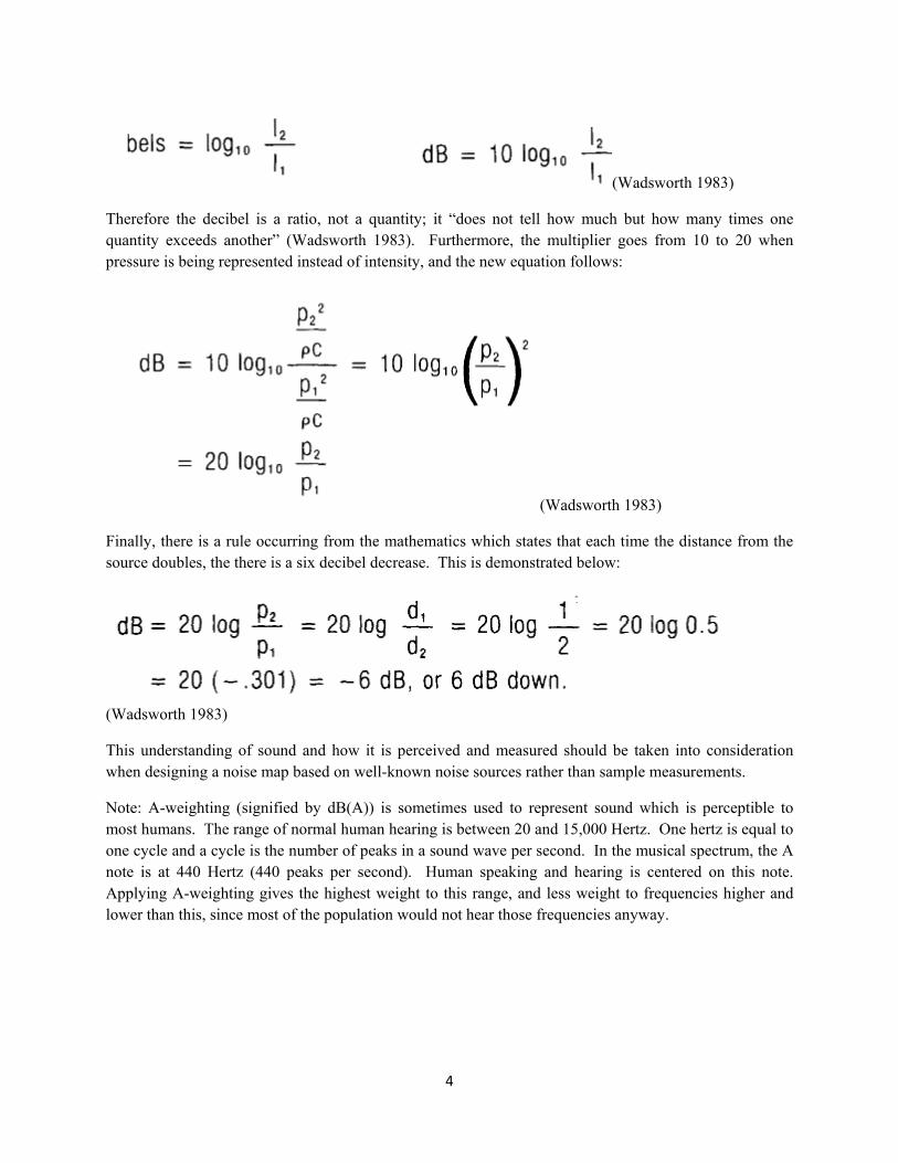
Therefore the decibel is a ratio, not a quantity; it “does not tell how much but how many times one quantity exceeds another” (Wadsworth 1983). Furthermore, the multiplier goes from 10 to 20 when pressure is being represented instead of intensity, and the new equation follows:

(Wadsworth 1983)

Finally, there is a rule occurring from the mathematics which states that each time the distance from the source doubles, the there is a six decibel decrease. This is demonstrated below:

(Wadsworth 1983)

This understanding of sound and how it is perceived and measured should be taken into consideration when designing a noise map based on well-known noise sources rather than sample measurements.

Note: A-weighting (signified by dB(A)) is sometimes used to represent sound which is perceptible to most humans. The range of normal human hearing is between 20 and 15,000 Hertz. One hertz is equal to one cycle and a cycle is the number of peaks in a sound wave per second. In the musical spectrum, the A note is at 440 Hertz (440 peaks per second). Human speaking and hearing is centered on this note. Applying A-weighting gives the highest weight to this range, and less weight to frequencies higher and lower than this, since most of the population would not hear those frequencies anyway.

5

2.2 Understanding Noise and Decibels Table 1 below exemplifies familiar sounds and their corresponding decibel levels and effects.

Table 1: Comparative Examples of Noise Levels (Comparative 2012)

6

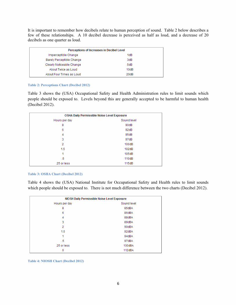
It is important to remember how decibels relate to human perception of sound. Table 2 below describes a few of these relationships. A 10 decibel decrease is perceived as half as loud, and a decrease of 20 decibels as one quarter as loud.

Table 2: Perceptions Chart (Decibel 2012)

Table 3 shows the (USA) Occupational Safety and Health Administration rules to limit sounds which people should be exposed to. Levels beyond this are generally accepted to be harmful to human health (Decibel 2012).

Table 3: OSHA Chart (Decibel 2012)

Table 4 shows the (USA) National Institute for Occupational Safety and Health rules to limit sounds which people should be exposed to. There is not much difference between the two charts (Decibel 2012).

Table 4: NIOSH Chart (Decibel 2012)

7

Table 5 shows the World Health Organization guidelines for noise levels (Future 1996). Note especially that the outdoor limit for schools is 55 decibels, and no nighttime limits are defined, although some universities have residences on their campuses. This is in keeping with ReMa’s noise measurements only recording daytime values.

Table 5: WHO Chart (Future 1996)

In 1996, the goals of the WHO and the END were “to phase out average exposure above 65 decibels, to ensure that at no point in time a level of 85 decibels should be exceeded coupled with the aim of ensuring that the proportions of the population exposed to average levels between 55 and 65 decibels should not increase and [to ensure that] exposure in quiet areas should not increase beyond 55 decibels” (Future 1996). The relevant law in the case of this thesis is that the outdoor noise level on the UJI campus should not exceed 55 dB(A).

8

2.3 Noise Data Collection Technique

2.3.1 Sampling Grids and Wireless Sensor Networks There are many elements in the process of noise mapping, and many choices to be made at each step. The measurement collection scheme must be devised to reflect different times of day and different parts of the study area. A regular grid is a common plan and can be drawn manually or selected by a software program, but some of the points may fall inside a building footprint. The choices are to take the measurement from the roof in the correct location, to move the location to the nearest possible spot on the ground or to eliminate the point altogether (Arana 2009). An additional method is to select major intersections instead of trying to use a geometrical grid (Yilmaz 2006).

Another element to consider is the source. Noise sources can be mapped as points or lines. While individual vehicles could be represented as points, traffic noise is generally modeled as a line representing the roadway. It is also possible to represent traffic as “a line of point sources” (De Muer 2003). Features such as air conditioning units, construction sites and other machinery usage can be modeled as points. Arana suggests that although lines can be more reliable for precise knowledge, a true evaluation of the sources requires using both points and line sources (Arana 2009). Another approach is to use an image of the study area and define the pixels of a noise source as a line, thereby creating a line source map from a point source map (Yilmaz 2006).

A study in Nigeria used a professional sound level meter to collect data, but instead of making noise maps, they quantified the areas according to areas in violation of allowed sound levels and returned results in the form of charts and action plans for various land use settings. “The selected areas of study are commercial centers, road junctions/busy roads, passenger loading parks, and high-density and low-density residential areas. The road junctions had the highest noise pollution levels, followed by commercial centers” (Oyedepo 2010)

2.3.2 Smart Phones It has been suggested that using citizens as sensors is a cheaper alternative to the methods of noise pollution data collection described above. What is the best way to achieve the kind of participation that would be necessary to build spatially and temporally rich noise databases? Garcia Marti et. al follow “gamification techniques to encourage users to participate using their personal smart phones” (Garcia Marti 2012). Using the concepts of “user status, access, power and stuff,” they have built a game for Android phones which entices users not only to play one time, but to become repeat or regular users (Garcia Marti 2012). Furthermore, an environment is created in which users want to include their friends, and their friends want to invite their friends, etc, thereby increasing the amount of participation The potential here to increase the size of a spatial and temporal noise pollution database far surpasses that of any other noise data collection method.

NoiseSPY was a project carried out Cambridge using Nokia mobile phones to collect data from bicycle couriers. The tests they ran to compare the Nokia N95 microphone sensors with Norsonic Noise meter on loan from the Cambridge city council returned very small discrepancy between the two. Their research indicates that “not only is the functionality of this personal environmental sensing tool engaging for users, but aspects such as personalization of data, contextual information, and reflection upon both the data and its collection, are important factors in obtaining and retaining their interest” (Kanjo 2009). However, as

9

long as the collection is only carried out by couriers, the validity of this statement is questionable. Perhaps gamification is a useful strategy for them, as well.

Zimmerman et. al. developed their own method of using smart phones to monitor residential noise. They identify several issues “including location of the phone (e.g. hand, pocket or backpack), modification of the detected sound by phone hardware and firmware (e.g. noise cancellation, low-pass filtering, automatic gain control), and power consumption limiting continuous monitoring duration” (Zimmerman 2011). By building a custom system, they bypassed the limitations of the smart phone audio performance. They supplemented their findings with customer surveys to learn how important noise pollution is to selecting a place to live and then to gage the effectiveness of their noise data presentation methods.

2.4 Noise Mapping Technique

2.4.1 Software Package Approach Many European member states have designed and implemented traffic noise prediction models, and the French method is recommended by the END. Beyond simply measuring noise, it calculates source and atmospheric propagation conditions (Arana 2009). There is also a variety of software programs which have models to predict noise using complex algorithms and parameters including weather conditions, reflecting and absorbing materials of surrounding structures, “angle of incidence, the wavelength and the distance between source, receiver and reflecting surface” (Arana 2009). Other parameters relate to road traffic, including “traffic velocity, start-stop conditions and road surface” (De Muer 2003). It is possible that the range of decibel levels measured will not vary greatly, but this can be deceivingly simplistic. There are algorithms available in these software models which can reveal interesting differences. Three examples of software programs are SoundPlan, Cadna/A and Lima Predictor (Arana 2009). Even more complex approaches have been taken to attempt to address the uncertainty which enters the equations at different steps. Assumptions made about parameters and conditions, measurements made at places which do not truly represent the noise in the surrounding area, the partial knowledge of imposing upper and lower limits to parameters and the data potentially lost when choosing line or point sources are all influences which are literally uncertain. De Muer and Botteldooren studied the applications of both a probability approach (Monte Carlo) and a possibility approach (Fuzzy Set) and found that both returned practical results, while the Fuzzy Approach made faster calculations (De Muer 2003).

In Navarre, Spain, researchers mapped six areas of roads in addition to the Agglomeration of the Region of Pamplona (ARP) using Cadna/A software. Their focus was to design action plans using “different prioritisation criteria concerning rank-based effectiveness measures (mainly the amount of people benefitting from them)” (Arana 2012).

10

2.4.2 Geostatistical Approach versus Noise Source Attenuation Approach An undisclosed interpolation method was used in GIS to make a noise map in Turkey. The researchers used both point and line sources and created the maps shown in Figure 1.

Figure 1: Point and Line Source Maps (Yilmaz 2006)

The maps above use highways as point and line sources for traffic noise in Turkey, interpolated with common GIS tools (Yilmaz 2006). These were designed for contiguous data such as air temperature or soil pH. Phenomena like that are spatially auto-correlated, meaning that nearby points are more similar to each other than more distant ones. Although this is also nominally true for noise, there is technically more going on than that. Sound propagation and combination behave differently than either temperature or soil pH.

The maps below use economic activities as point sources and roads as line sources in Brazil. A new set of GIS based tools were developed by researchers in Brazil using the sound attenuation equations and concepts described earlier (Piedade 1999). An example of the maps created with this approach is shown in Figure 2 below. Note that these maps are at a much larger scale (showing a smaller area) than those pictured above. This is because the sound attenuation rules state that sound decreases by six decibels every time the distance from the source doubles.

Figure 2: Point and Line Source Maps (Piedade 1999)

11

3. Data and Methods

3.1 Methods of noise measurement collection

3.1.1 Noise Droid This is an application developed by the Institute for Geoinformatics (IFGI) at the University of Muenster, Germany as part of the Open Noise Map project. It is for use by Android smart phones to gather noise pollution data. Some of the highlights of the application are described on the website:

It supports manual, automatic, event-based and series mode measurements and presents all collected measurements in a list or on a map. Details can be shown and the list can be sorted and filtered by a number of criteria. Additionally the users can export measurements to the Open Noise Map community and import from community measurements (Noise 2013).

Noise Droid is equipped with a noise quality assessment, which comes with its open source software and is therefore available with other applications developed using its code (Garcia Marti 2012).

3.1.2 Noise Battle This is a game developed at the Institute of New Imaging Technology at the Universitat Jaume I in Castellon, Spain. Using the basic program from Noise Droid, Noise Battle turns the application into a game for multiple users. Gamification techniques are useful for encouraging citizen participation in Volunteered Geographic Information(VGI) gathering (Garcia Marti 2012). It has an avatar visible on the screen, and the city is divided into cells for easy classification into the game point system and into the database. That this application is a game offering rewards to users who can become repeat users and who, by word of mouth (or social media) can spread the game to friends and friends of friends makes it a potentially superior tool to grow a database of noise pollution which is comprehensive in both spatial and temporal dimensions.

3.1.3 Sound Meter This is an application available from Google Play for Android phones developed by “Android Boy.” It is part of a series of Smart Tools including a compass, ruler, measure, etc. The application uses the smart phone microphone to measure sound pressure level in decibels. Some phones are calibrated to measure in dB(A), the A-weighted system most commonly used. It is noted that smart phone microphones “were aligned to human voice (300-3400Hz, 40-60dB)” (Sound 2012). This accounts for the upper limit of measurement set at 86 decibels on the Samsung Galaxy Y. The display is a round meter with three red lines for minimum, mean and maximum and a history line chart below, both showing real time noise levels. The average rating for the application is 4.3 out of 5, with 28,808 users giving it 5 stars.

12

3.2 Data collection fieldwork

3.2.1 Noise receivers The base data available for this project consists of several sets of sound measurements at 66 location points across the UJI campus in a (mostly) regular grid. These points act as the receivers of sound in this study. Points that would have fallen on top of buildings were moved to a location on the ground nearby. These measurements were taken between November 26 and December 3, 2012 by a private contracting company called ReMa. The measurements are taken during four different intervals of the day. The reference system for the points is a grid of numbers one to six along two axes. This was georeferenced to the campus basemap in GIS by the author.

Many difficulties were encountered during the fieldwork. The plan was to collect sound measurements alongside the professional contractors from ReMa, using a smart phone. ReMa equipment was on a tripod approximately one and a half meters high, and came with a wind-muffling foam cover for the microphone.

The Samsung Galaxy Y, purchased specifically for the purpose of this thesis, came with neither of these accessories. The choices were to hold the phone at the same height or to set it on the ground. In some locations, manicured bushes provided a satisfactory surface above the ground to place the phone. Whenever the phone was not being held, it was placed on a folder on top of the ground or bush, so that it did not directly touch the surface. The fourth day a small tripod was acquired and used thereafter.

ReMa recorded sound levels for five minutes at a time at each location during four different intervals of the day. They used a CESVA SC-20c Sound Level Meter. The range of its recording capability is 23 to 140 dB. It records several functions. L10 and L90 are the standard deviations of the measurements. LeqT is the mean, MaxLF is the absolute maximum and MaxLeq1m is the mean decibel level for the sound recorded during the loudest continuous minute. The device is a type one sound meter following UNE –EN 60651 and UNE – EN 60804 and was calibrated using the CB006 Class 1 Acoustic Calibrator (CESVA 2011).

The author had the application open and ready to begin recording simultaneously at the touch of a button. It displays the mean and maximum sound levels in decibels. The Noise Battle application records sound for 10 seconds. In order to save the measurement, one has to touch the screen in exactly the right place, in the area below the avatar. If not touched correctly, either nothing happens or the view changes and one must swipe the screen to find the current location again. When it does happen correctly, a box pops up with a button to “Send Data.” Once this is touched, one of three things happens.

• Onscreen message: “Measurement sent correctly.”

• Onscreen message: “INVALID_MEASURE_BLOCK”

• No onscreen message visible

After three incidents where the author was unsure of whether the measurement was being recorded, the author began writing the data down each time. Again, both mean and maximum were recorded.

13

Next the Noise Droid application was opened and recording begun at the touch of a button. It records for eight seconds and displays minimum as well as mean and maximum. Saving the measurement is easily accomplished with a touch of the “Send Data” button which is constantly available on the screen. Unfortunately, when the data from Noise Droid was downloaded, the author found that only the mean had been saved at each measurement point. Two days of fieldwork were left at that point, so the author recorded the measurements by hand, but it was not enough maximum data to usefully compare to the other applications. Additionally, many of the measurements did not upload successfully, although the GPS coordinates did.

The final step was to open the Sound Meter application, which begins measuring immediately and continues until stopped manually. The author left it measuring until the ReMa associate stopped his recording. Sound Meter displays the minimum, mean and maximum, but there is no way to save the data; it must be written down. Therefore, all three measurements were recorded for each measurement point.

During the fieldwork collection, the author observed that the professional equipment was reading a consistently lower decibel level than the smart phone applications. It is assumed that the display of both devices was of the current running average. If this was so, then the smart phone appeared to be more sensitive to changing sounds such as people walking past or cars driving by. It could be that the professional sound meter simply was not constantly displaying the current running average level and was actually displaying some calculation of one of its other functions instead. Later comparisons of the data will provide more information. Finally, the upper limit appears to be 86 dB(A), as specified by the application description available online and then observed during fieldwork as well as tested by yelling into the microphone.

The first day, Monday, November 26, 2012, recordings were taken from 11:15 to 20:00. Besides becoming familiar with the equipment and procedures, nothing remarkable occurred. On the second day, measurements were taken from 08:00 until 22:00. It began to rain lightly twice, once around 09:00 for about thirty minutes and again around 15:00 for about an hour. Both incidences halted the fieldwork until the raining stopped. On the third day, measuring began at 08:00 but was abandoned by 11:00 due to high winds of between 32 and 42 kilometers per hour. These winds continued for the rest of the day and the next day and no fieldwork was attempted. Measurements resumed on Friday, November 30, 2012, which will be called the fourth day. That day fieldwork was carried out from 08:00 until 22:00. Work continued the following Monday, December 3, 2012, called the fifth day, at 08:00. Since the remaining number of points to be measured was dwindling, work was not constant all day. Instead, the final measurements for intervals one, two and three were recorded with breaks in between. Fieldwork was concluded on the sixth day, Tuesday, December 4, 2012 from 19:30 until 22:00.

Wind gusts created significantly skewed noise measurements. During a wind gust where no actual sound could be heard, the sound level rose to and stayed at 86 decibels until the gust died down. Two of these such recordings were noted, while all the measurements taken on the morning of Wednesday, November 28, 2012 are believed to be skewed. This will be examined later on.

ReMa was unable to produce noise maps for the 2012 data in time for comparison in this research.

14

3.2.2 Noise sources The author walked around each building on the campus, making note of noise sources. The following day, a Samsung Galaxy SII (GT-9100) was borrowed from a colleague to measure the sound levels at each of these sources. Noises recorded as point features were described as fans, vents, bicycle stations, construction machinery, fountains, maintenance equipment, gardening saw, high pitched sound, and ‘peligro.’ Many of the areas from which loud noise was emanating were marked with a sign reading ‘peligro,’ which is Spanish for danger. Noises recorded as polygon features were described as cafes with talking, cafes with talking and music, vent system over water, racquet ball court, bus stop, and tram stop. Later it was found that interpolating between polygon sources left the insides of the polygons with no data, so these areas were redrawn as lines or a crisscross of two or more lines. A total of 32 noise point sources and nine noise line sources were recorded as data.

The author bicycled the surrounding areas of UJI included within the study area and recorded speed limits. The individual roads, numbering more than 260, were grouped according to speed limit and then further grouped according to the decibel level associated with that speed limit. Roads with speed limits of 30 – 50 kilometers per hour (kph) with mostly passenger vehicle traffic were grouped together and rated at 75 decibels. This classification contains most of the roads within and surrounding the UJI campus. Only two roads with speed limits of 60 kph are within this area, and in consideration of the occasional medium to heavy trucks, these were rated at 80 decibels. The Autopista del Mediterrani is the only 120 kph road and due to its heavy traffic including medium and heavy trucks, was rated at 90 decibels (Michael 2013). All the roads that fall within these three decibel ratings were grouped together and merged into three road noise source features.

Although the END specifies that noise generated by people does not fall within its statutes, the author felt that including all perceptible noise sources in the data collection would be the best strategy for making the most accurate noise map. Of course, if the noise levels are higher than the law permits in an area where a busy cafe is the culprit, it will not be treated as a problem to be addressed by UJI. Only traffic, construction and heavy machinery-type noise sources are under investigation for legal repercussions.

Later during the research, the author used four features placed at the corners of the study area in order to force the output of certain tools to use its extent instead of that of the points. Later it was found that it was also possible to set the output extent in the environment settings of a map document, but it was more practical working with the extra points.

15

4. Results: Can crowdsourced noise measurements help provide useful information to noise mapping?

4.1 Comparisons of smart phone applications to CESVA sound level meter with ANOVA The first objective of this thesis is to determine whether sound measurements taken using a smart phone are comparable to those taken professionally using calibrated instruments. The “comparable” characteristic in question here is quality, and the question is: are the measurements similar enough that they can be considered of equal quality? Additionally, if the measurements of the smart phone are different from those of the professional sound meter, are they consistently so? In other words, if they are consistently x decibels higher, then can x be subtracted from all of them to arrive at values similar to those of CESVA?

One way to compare data is to use a statistical test called Analysis of Variance (ANOVA). This test can be applied to several datasets, thereby comparing them all at once. ANOVA tests the diversity of the means of each dataset by analyzing their variances (Weisstein 2012). There are several ways to measure the variance. The simplest is just the range, which is the maximum value minus the minimum value. A more sophisticated measure of variance is called the sample variance. In this case, the mean of the dataset is subtracted from each value and then squared. The sum of the squares is then divided by the number of values in the dataset minus one (also known as ‘degrees of freedom’). The resulting value represents the unbiased estimation of the variance of the data values (Jones 2012).

ANOVA compares the means and computes a ‘P-value,’ which is the “probability that a variate would assume a value greater than or equal to the observed value strictly by chance” (Weisstein 2012). The null hypothesis is that all the means of the datasets will be the same. If the p-value is less than the Alpha value (set at 0.05 (5%) for a 95% confidence interval), then the null hypothesis must be rejected. When this happens, the conclusion is that there is a statistically significant difference between the datasets. The results are reported as means, variances , the F-Statistic used to run the test, and the resulting p-value in parentheses. An assumption of ANOVA is that the datasets being compared are normally distributed, but because this data is in a logarithmic scale, it is already somewhat so.

Using Microsoft Excel 2007, the author has tested three groups (10 subgroups) of different combinations of the data with the ANOVA statistical test. ReMa associates recorded sound levels at sixty-six locations across the campus using the professional CESVA Sound Level Meter, for four different intervals of the day. The first interval is from 08:00 to 11:15, the second from 11:15 to 14:30, the third from 13:30 to 18:45 and the fourth from 18:45 to 22:00. The dataset recorded by ReMa will be referred to from now on as CESVA. The intervals will be referred to as 1int, 2int, 3int and 4int. Simultaneously, the author recorded sound levels using three different smart phone applications, which produced three more datasets. These will be referred to by the name of the application used to record them: Noise Droid, Noise Battle and Sound Meter, and these together with CESVA will be referred to as methods. All the methods except for Noise Droid recorded a mean decibel level and a maximum decibel level. The mean decibel level is the average of all the decibel levels recorded for the period of time the method was recording. The maximum decibel level is the one single highest decibel level recorded during that time. The mean represents the entire period, while the maximum could represent as little as a second. Hereafter, the word

16

measurement refers to either the mean or the maximum decibel level for a given method, according to each section heading.

Hence, here is the organization of the analysis which follows:

Means First Interval Second Interval Third Interval Fourth Interval

Maximums First Interval Second Interval Third Interval Fourth Interval

All measurements for all intervals together by method Means Maximums

It is said that a picture is worth a thousand words. One way to compare these measurements would be to write a paragraph for each of the 66 measurement locations, discussing the decibel levels reported by the four different methods. This would be an incredibly tedious report to read:

The next measurement to be examined is number 42. It is located on the sidewalk at grid point 4, 9, on the north side of the tram guide way, about halfway between the campus entrance and the tram stop. During the first interval, the Noise Droid mean was 60.5 decibels, the Noise Battle mean was 56.7 decibels, the Sound Meter mean was 63 decibels and the CESVA mean was 49.8 decibels. The Noise Battle maximum was 73.7 decibels, the Sound Meter maximum was 73 decibels and the CESVA maximum was 60.8 decibels. During the second interval, the Noise Droid mean was 73.7 decibels, the Noise Battle mean was 64 decibels, the Sound Meter mean was 82 decibels and the CESVA mean was 56.2 decibels. The Noise Battle maximum was 76.7 decibels, the Sound Meter maximum was 86 decibels and the CESVA maximum was 71.3 decibels. During the third interval, the Noise Droid mean was 66 decibels, the Noise Battle mean was 60.8 decibels, the Sound Meter mean was 74 decibels and the CESVA mean was 59 decibels. The Noise Battle maximum was 72.7 decibels, the Sound Meter maximum was 86 decibels and the CESVA maximum was 73.3 decibels. During the fourth interval, the Noise Droid mean was 61.7 decibels, the Noise Battle mean was 61.9 decibels, the Sound Meter mean was 73 decibels and the CESVA mean was 58.2 decibels. The Noise Battle maximum was 74.4 decibels, the Sound Meter maximum was 86 decibels and the CESVA maximum was 72.7 decibels.

That is already boring and difficult to process. Imagine reading 65 more. Attaining meaning from that wordy list would not be easy, and describing the summary statistics and other observable relationships would be difficult. In fact, almost no amount of spatial information is presented that way. For the benefit of the reader and in the interests of the clearest elucidation of the comparisons, graphic and spatial visualizations are presented below.

For each of these test subgroups, two visuals will be provided to illustrate the differences among the datasets. The first is a scatter plot graph showing decibels on the y-axis and matched measurements for

17

each location on the x-axis. In each case, the CESVA or the first interval measurements are ordered least to greatest, with the measurements from the other datasets matched above or below, depending upon whether the measurement is lower or higher. The second graphic is a bar chart showing selected summary statistics in decibels including mean, mode, variance, minimum, median and maximum for each dataset being compared. The mode is the value that was recorded most often during the measurement time. It is interesting when it differs from the mean, since the mean is influenced by the extremes while the mode is not. Therefore, the mode can represent what the mean might have been had it not been for a single peak event (unless the extremes balance each other out evenly.) When the mean and median are similar, it is close to a normal distribution (Histograms 2013). Brief commentary will follow each visual, while the interpretation is saved for the discussion afterward. For the interval comparisons of means, maps will also be presented comparing the sound levels reported by the four methods in a spatial layout.

The most important thing to keep in mind while examining these comparisons is that decibels are a logarithmic scale. An increase of 10 decibels is perceived by the human ear as doubly loud. For example, if the smart phone application records a 75 decibel level and the professional sound level meter records 65 decibels, the smart phone is claiming that the location being measured is twice as loud. Therefore, while the differences between the values in these datasets may seem small, these measurement devices are depicting two very different representations of the real world.

18

4.1.1 Means

4.1.1.1 First Interval

45

50

55

60

65

70

75

80

85

Decib

els

Matched measurements for each location

1st Interval Means by Method

Noise DroidNoise BattleSound MeterCESVA

Figure 3: Graph of First Interval Means by Method

Figure 3 shows that Noise Battle and Noise Droid measurements are fairly similar for all observations, with a few extra highs for Noise Droid and a few extra lows for Noise Droid. Sound Meter is most consistently higher than CESVA , but follows the same progression of least to greatest.

Mean Variance F-StatisticNoise Droid 64 34Noise Battle 62 19Sound Meter 70 38CESVA 57 26

64.65(6.93E-31)

Table 6: ANOVA First Interval Means by Method

Table 6 shows the results of ANOVA for the first subgroup. The value of the statistical test used to compare the means is 64.65. The p-value is less than 5%, so for the first interval, the means of the four different methods are statistically significantly different. Noise Battle and Noise Droid have similar means but very different variances. Noise Battle and CESVA have similar means and less different variances. Sound Meter and Noise Droid have similar variances but different means. The CESVA mean is less than the others, and the Sound Meter mean is greater than the others.

19

0 20 40 60 80 100

Mean

Mode

Variance

Minimum

Median

Maximum

Decibels

Sum

mar

y St

atist

ics1st Interval Means by Method

CESVASound MeterNoise BattleNoise Droid

Figure 4: Graph of Summary Statistics First Interval Means by Method

Figure 4 shows summary statistics for the four methods of sound measurement. The Sound Meter measurements are consistently higher than the rest. The range for maximums is high, while minimums are fairly close together. The medians are similar with the exception of Sound Meter at 10 decibels higher. Although the means are not that dissimilar, the variances differ more greatly than any other statistic. The modes for each method are close to the means for the same method. Figure 5 shows that the variations in spatial locations between highs and lows in the four datasets are apparently random.

Figure 5: Maps of First Interval Means

20

Figure 6: Maps of Kriging First Interval Measurements

Figure 6 shows the results of kriging interpolation for the first interval measurements of each of the four methods. Sound Meter has the highest decibels levels, CESVA has the lowest, and Noise Droid is similar to Noise Battle.

21

4.1.1.2 Second Interval

45

50

55

60

65

70

75

80

85

Decib

els


2nd Interval Means by Method


Figure 7: Graph of Second Interval Means by Method

As is visible in Figure 7, the second interval is nearly identical to the first, with fewer Noise Droid extremes on the high end. Noise Droid and Noise Battle measurements lie in the same range, slightly above the CESVA measurements.


63.04(2.19E-30)

Table 7: ANOVA Second Interval Means by Method

Table 7 shows the results of ANOVA for this subgroup. The value of the statistical test used to compare the means is 63.04. The p-value is less than 5%, so for the second interval, the means of the four different methods are statistically significantly different. The Noise Droid and Noise Battle means are the same but with very different variances. The Sound Meter and CESVA means are both different from each other and different from the other two applications. The Noise Droid and CESVA variances are the closest together. The CESVA mean is less than the others, and the Sound Meter mean is greater than the others.

22

0 20 40 60 80 100

Mean

Mode

Variance

Minimum

Median

Maximum

Decibels

Sum

mar

y St

atist

ics2nd Interval Means by Method


Figure 8: Graph of Summary Statistics Second Interval Means by Method

Figure 8 shows that Sound Meter has the highest statistics again, except the Noise Droid minimum is higher. Again, Noise Battle has the smallest variance and the variances are all very different. The modes, especially CESVA, are lower than the means. Noise Battle and Noise Droid share the same mean and nearly the same median. Figure 9 shows that the variations in spatial locations between highs and lows in the four datasets are apparently random.

Figure 9: Maps of Second Interval Means

23

Figure 10: Maps of Kriging Second Interval Measurements


24

4.1.1.3 Third Interval

45

50

55

60

65

70

75

80

85

Decib

els


3rd Interval Means by Method


Figure 11: Graph of Third Interval Means by Method

In Figure 11, it is apparent that the measurements are more consolidated along the same plane, congruent to that of the CESVA progression. This is the interval during which the Sound Meter measurements are closest to the rest, with fewer extremes and smaller differences. Noise Battle still drops below CESVA in a few of the same spots as the morning intervals.


46.08(6.71E-24)

Table 8: ANOVA Third Interval Means by Method

Table 8 shows the results of ANOVA for this subgroup. The value of the statistical test used to compare the means is 46.08. The p-value is less than 5%, so for the third interval, the means of the four different methods are statistically significantly different. The Noise Droid and Noise Battle means are almost the same but with different variances again. The Sound Meter and CESVA means are again both different from each other and from the other two methods. The CESVA mean is less than the others, and the Sound Meter mean is greater than the others.

25

0 20 40 60 80 100

Mean

Mode

Variance

Minimum

Median

Maximum

Decibels

Sum

mar

y St

atist

ics3rd Interval Means by Method


Figure 12: Graph of Summary Statistics Third Interval Means by Method

In Figure 12, it can be seen that Sound Meter is still the leader in high values, but not by as large a difference as in earlier intervals. Noise Droid recorded the same maximum as Sound Meter and Noise Droid and Noise Battle recorded the same mode. The variances for all but Noise Battle are close this time. CESVA has the lowest statistics except for variance and mode. Figure 13 shows that the variations in spatial locations between highs and lows in the four datasets are apparently random.

Figure 13: Maps of Third Interval Means

26

Figure 14: Maps of Kriging Third Interval Measurements


27

4.1.1.4 Fourth Interval

45

50

55

60

65

70

75

80

85

Decib

els


4th Interval Means by Method


Figure 15: Graph of Fourth Interval Means by Method

In Figure 15, it can be seen that the distribution is similar to the previous interval, but with more high decibel level extremes in the Sound Meter dataset. The three smart phone applications follow the same general progression as CESVA, only 10 to 20 decibels higher. It is important to keep in mind that a 10 decibel increase sounds twice as loud and a 20 decibel increase sounds four times as loud. Therefore, the sound scheme recorded by the three phone methods is significantly different than that recorded by the professional CESVA.


57.01(2.36E-28)

Table 9: ANOVA Fourth Interval Means by Method

Table 9 shows the results of ANOVA for this subgroup. The value of the statistical test used to compare the means is 57.01. The p-value is less than 5%, so for the fourth interval, the means of the four different methods are statistically significantly different. As before, the Noise Droid and Noise Battle means are the same, but this time the variances are closer. The Sound Meter and CESVA means are different from each other and the others but the variances are close. The CESVA mean is less than the others, and the Sound Meter mean is greater than the others.

28

0 20 40 60 80 100

Mean

Mode

Variance

Minimum

Median

Maximum

Decibels

Sum

mar

y St

atist

ics4th Interval Means by Method


Figure 16: Graph of Summary Statistics Fourth Interval Means by Method

In Figure 16 it can be seen that the variances are closer than any other interval so far, yet ANOVA revealed they are still statistically different. This time the Sound Meter maximum was surpassed by Noise Droid. CESVA values are lower than the rest, except for the variance. The means are higher than the modes. Figure 17 shows that the variations in spatial locations between highs and lows in the four datasets are apparently random.

Figure 17: Maps of Fourth Interval Means

29

Figure 18: Maps of Kriging Fourth Interval Measurements


30

4.1.2 Maximums

4.1.2.1 First Interval For this section, there is no Noise Droid dataset since maximums were not recorded by that application. It remains in the legend to preserve the consistent color scheme.

50

55

60

65

70

75

80

85

90

95

Decib

els


1st Interval Maximums by Method


Figure 19: Graph of First Interval Maximums by Method

Figure 19 shows the maximums for each dataset during the first interval. Sound Meter records the highest values but the upper limit is only 86 decibels, so any sound louder than that will still be recorded at 86. Note that the CESVA values which correspond to these maximums range from 74 to 83. Noise Battle measurements are again concentrated in a band mostly above the CESVA values, with a few low extremes.

Mean Variance F-StatisticNoise Battle 72 23Sound Meter 82 38CESVA 70 54

61.67(1.96E-21)

Table 10: ANOVA First Interval Maximums by Method

Table 10 shows the results of ANOVA for this subgroup. The value of the statistical test used to compare the means is 61.67. The p-value is less than 5%, so for the first interval, the maximums of the four different methods are statistically significantly different. The Noise Battle and CESVA means are similar, but different from the Sound Meter mean. The CESVA mean is less than the others, and the Sound Meter mean is greater than the others.

31

0 20 40 60 80 100

Mean

Mode

Variance

Minimum

Median

Maximum

Decibels

Sum

mar

y St

atist

ics1st Interval Maximums by Method


Figure 20: Graph of Summary Statistics First Interval Means by Method

Figure 20 displays the summary statistics for the first interval maximums for each method. Sound Meter has a much higher median, mode and mean, while Noise Battle’s minimum is highest and CESVA’s variance is greatest. The modes are higher than the means. The mode for Sound Meter is the upper limit and the same as the maximum. The variances differ widely – at 23, 38 and 54.

32

4.1.2.2 Second Interval

50

55

60

65

70

75

80

85

90

95

Decib

els


2nd Interval Maximums by Method


Figure 21: Graph of Second Interval Maximums by Method

In Figure 21, it can be seen that more of the Noise Battle measurements are higher compared to CESVA than in the last interval. There are also three measurements lower than CESVA at the lower end. Also, around one-third of the Sound Meter measurements are at the upper limit of 86, and nearly one-half are above 80 decibels. For the first time so far, all the Sound Meter measurements are higher than the CESVA values. This is due to extremely high winds the day the measurements were taken and is discussed in detail in another section.


56.14(5.79E-20)

Table 11: ANOVA Second Interval Maximums by Method

Table 11 shows the results of ANOVA for this subgroup. The value of the statistical test used to compare the means is 56.14. The p-value is less than 5%, so for the second interval, the maximums of the four different methods are statistically significantly different. Each mean in this comparison is different from the others. The CESVA mean is less than the others, and the Sound Meter mean is greater than the others.

33

0 20 40 60 80 100

Mean

Mode

Variance

Minimum

Median

Maximum

Decibels

Sum

mar

y St

atist

ics2nd Interval Maximums by Method


Figure 22: Graph of Summary Statistics Second Interval Maximums by Method

Here in Figure 22, the CESVA mode is much lower than Noise Battle or Sound Meter, with a 20 decibel difference (four times as loud). Again, the Sound Meter mode is the same as the maximum, and these are higher than the others. The variances are quite different, and the modes are very close to the means.

34

4.1.2.3 Third Interval

50

55

60

65

70

75

80

85

90

95

Decib

els


3rd Interval Maximums by Method


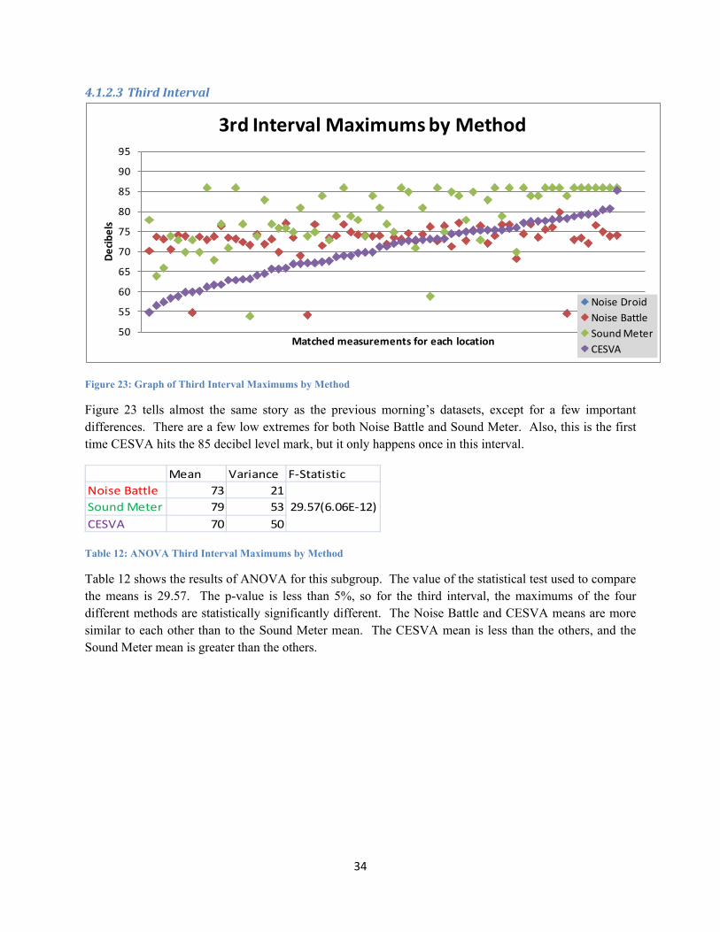
Figure 23: Graph of Third Interval Maximums by Method

Figure 23 tells almost the same story as the previous morning’s datasets, except for a few important differences. There are a few low extremes for both Noise Battle and Sound Meter. Also, this is the first time CESVA hits the 85 decibel level mark, but it only happens once in this interval.


29.57(6.06E-12)

Table 12: ANOVA Third Interval Maximums by Method

Table 12 shows the results of ANOVA for this subgroup. The value of the statistical test used to compare the means is 29.57. The p-value is less than 5%, so for the third interval, the maximums of the four different methods are statistically significantly different. The Noise Battle and CESVA means are more similar to each other than to the Sound Meter mean. The CESVA mean is less than the others, and the Sound Meter mean is greater than the others.

35

0 20 40 60 80 100

Mean

Mode

Variance

Minimum

Median

Maximum

Decibels

Sum

mar

y St

atist

ics3rd Interval Maximums by Method


Figure 24: Graph of Summary Statistics Third Interval Maximums by Method

In Figure 25, it can be seen that the CESVA mode and mean are very close to Noise Battle. The variances of CESVA and Sound Meter are uncommonly close, with that of Noise Battle far below. The Sound Meter mode and maximum are still at 86, and this time the CESVA maximum is close behind at 85 but the mode is 10 decibels lower. The means are lower than the modes in this interval.

36

4.1.2.4 Fourth Interval

50

55

60

65

70

75

80

85

90

95

Decib

els


4th Interval Maximums by Method


Figure 25: Graph of Fourth Interval Maximums by Method

Figure 26 shows that the fourth interval Sound Meter measurements have dropped quite a bit, and while there are still many above 80 decibels, there are more in the 70 to 80 range. For the second time, none of the Sound Meter values are below those of CESVA. Noise Battle stays in the usual range with only two extreme lows this interval. There is also an abnormality which may be attributed to human error. There is one CESVA measurement at 93 decibels, which is nine decibels (almost twice as loud) as its next highest measurement. It is most likely that some interference occurred with the microphone to cause this extremely high measurement. Unlike the smart phone applications, the CESVA’s upper limit is not 86decibels, but 137, so it is possible that this was the actual maximum recorded at the time.


30.63(2.71E-12)

Table 13: ANOVA Fourth Interval Maximums by Method

Table13 shows the results of ANOVA for this subgroup. The value of the statistical test used to compare the means is 30.63. The p-value is less than 5%, so for the fourth interval, the maximums of the four different methods are statistically significantly different. Again, the Noise Battle and CESVA means are more similar to each other than to the Sound Meter mean. The CESVA mean is less than the others, and the Sound Meter mean is greater than the others.

37

0 20 40 60 80 100

Mean

Mode

Variance

Minimum

Median

Maximum

Decibels

Sum

mar

y St

atist

ics4th Interval Maximums by Method


Figure 26: Graph of Summary Statistics Fourth Interval Maximums by Method

Figure 26 displays the abnormal CESVA maximum of 93 decibels, surpassing the Sound Meter maximum in what may have been a human error. This number raises the CESVA variance at the same time, pulling its value well above the other methods as well. In the rest of the statistics, Sound Meter is still very much the leader in high values. The Noise Battle mode and mean are close.

38

4.1.3 All measurements for all intervals together by method

4.1.3.1 Means

45

50

55

60

65

70

75

80

85

Decib

els


Means


Figure 27: Graph of All Means by Method

Figure 27 shows all 264 measurements (66 for each of the four intervals) for each of the four methods. They are organized by CESVA least to greatest. The majority of smart phone measurements are above those of the professional sound meter. Most of the Noise Droid and Noise Battle measurements are 5 to 10 decibels higher (10 is twice as loud), with the high extremes as much as 20 to 25 decibels higher (20 is four times as loud). Most of the Sound Meter measurements are 10 to 15 decibels higher and the high extremes are up to 30 decibels louder. None of the Sound Meter means are lower than CESVA. In the upper range of CESVA measurements, there are several Noise Droid and Noise Battle measurements that are lower than the CESVA measurements, and most are within 10 decibels less (half as loud).


226.06(1.3E-112)

Table 14: ANOVA All Means by Method

Table 14shows the results of ANOVA for this subgroup. The value of the statistical test used to compare the means is 226.06. The p-value is far less than 5%, so the entire group of means for the four different methods are statistically significantly different. The Noise Droid and Noise Battle means are the same. The Sound Meter and CESVA means are different both from each other and from the other two methods. The CESVA mean is less than the others, and the Sound Meter mean is greater than the others.

39

0 20 40 60 80 100

Mean

Mode

Variance

Minimum

Median

Maximum

Decibels

Sum

mar

y St

atist

icsMeans

CESVA

Sound Meter

Noise Battle

Noise Droid

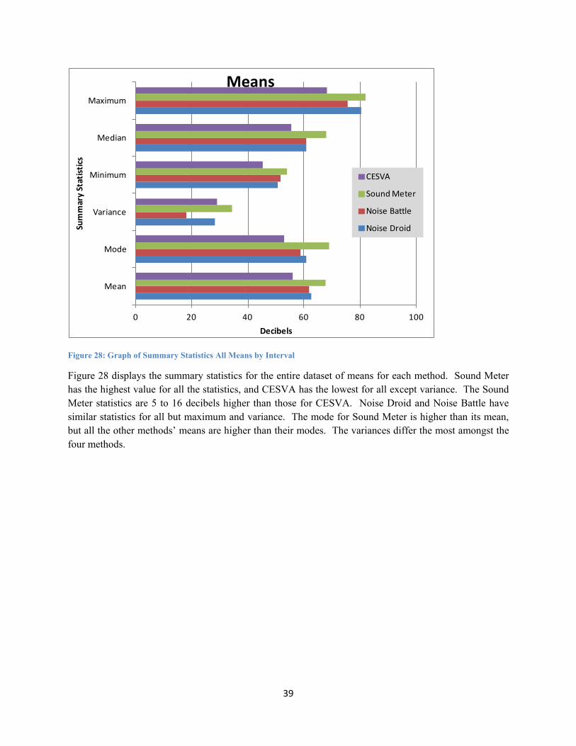
Figure 28: Graph of Summary Statistics All Means by Interval

Figure 28 displays the summary statistics for the entire dataset of means for each method. Sound Meter has the highest value for all the statistics, and CESVA has the lowest for all except variance. The Sound Meter statistics are 5 to 16 decibels higher than those for CESVA. Noise Droid and Noise Battle have similar statistics for all but maximum and variance. The mode for Sound Meter is higher than its mean, but all the other methods’ means are higher than their modes. The variances differ the most amongst the four methods.

40

4.1.3.2 Maximums

50

55

60

65

70

75

80

85

90

95De

cibel

s


Maximums


Figure 29: Graph of All Maximums by Method

Figure 29 shows all the maximum values from all four intervals combined into one dataset for each method except for Noise Droid, the software for which did not upload maximums. The datasets are matched to the progression of CESVA values from least to greatest. The Noise Battle measurements are all in roughly the same range, from 70 to 77 decibels. The majority of them are above the CESVA measurements, although several are below and a few are very far below. Unlike the means, a few of the Sound Meter maximums are below those for CESVA.


168.98(9.07E-62)

Table 15: ANOVA All Maximums by Method

Table 15 shows the results of ANOVA for this subgroup. The value of the statistical test used to compare the means is 168.98. The p-value is less than 5%, so the entire group of maximums for the four different methods are statistically significantly different. The mean of Noise Battle is similar to CESVA but different from Sound Meter, which is also different from CESVA. The CESVA mean is less than the others, and the Sound Meter mean is greater than the others.

41

0 20 40 60 80 100

Mean

Mode

Variance

Minimum

Median

Maximum

Decibels

Sum

mar

y St

atist

icsMaximums


Figure 30: Graph of Summary Statistics All Maximums by Method

Figure 30 displays the summary statistics for all the maximums for each interval by each of the three methods whose software uploaded maximum values. The possibly erroneous CESVA maximum of 93 decibels causes CESVA’s maximum and variance to be higher than that of the usual leader, Sound Meter. Sound Meter leads in the other statistic, by as much as 23decibels. The Sound Meter and Noise Droid modes are higher than their means, while the CESVA mean is higher than its mode.

42

4.2 Comparisons of smart phone applications to CESVA sound level meter with t-Tests In the previous section it was shown through the ANOVA testing that there is a statistically significant difference between the four test groups - sound measurements taken using the three smart phone applications and the professional sound level meter. In this section the author uses a variety of tools to compare only two datasets at a time in order to show exactly where these differences lie. Instead of looking at each interval separately, the full set of measurements for all four intervals are combined as in the final two ANOVA analyses. Each of the smart phone application datasets is compared to the CESVA dataset in a Student’s t-Test (also known as a one-way analysis of variance test), run in Microsoft Excel 2007, with the results reported followed by a brief commentary. First the t-Test: Two-Sample Assuming Equal Variances was run, and if the variances are not equal, the t-Test: Two-Sample Assuming Unequal Variances was run. The results are reported as means, variances , the t-Statistic used to run the test, and the resulting p-value in parentheses. When the p-value is less than the 0.05 (5%) Alpha (for a 95% confidence interval), the null hypothesis that the means are the same must be rejected and the conclusion is that the means are statistically significantly different. An assumption of t-Tests is that the datasets being compared are normally distributed, but because this data is in a logarithmic scale, it is already somewhat so.

For this analysis, the difference between each paired measurement has been calculated and plotted with the smart phone and CESVA datasets. In each instance, the difference is the smart phone measurement minus the CESVA measurement. The scatter plots are organized by the difference value from least to greatest, with the paired measurements above them on the same scale.

To validate the smart phone measurements against those taken by the CESVA, the sets are plotted against each other in a scatter plot. CESVA is the “measured decibel level” on the x-axis and the smart phone application is the “predicted decibel level” on the y-axis. The scale is the same for both axes, from 45 to 85 decibels for the means comparisons and from 50 to 90 decibels for the maximums comparisons. The blue line is the 45° degree line which, if the points fall along it, represents a one to one relationship and would validate the accuracy of the “prediction.” The black line is the actual linear trend line for the smart phone data. Comparing the two both illustrates and quantifies the tendency of inaccuracy recorded by the smart phones compared with the professionally calibrated sound level meter.

For further illustration, a histogram of each dataset is presented, with frequency on the y-axis and decibels on the x-axis. The scale of zero to 160 for frequency is used consistently for easy, unbiased visual comparison. Note that the way the histogram organizes the values may be misleading. Each value is rounded up and placed in a bin, and the numbers labeling the bins on the x-axis denote the highest value allowed in that bin. In other words, numbers from -10 to -5 fall into the -5 bin, and numbers from -4.9 to zero fall into the zero bin. For example, a value of -5.5 falls into the -5 bin, a -4.5 value falls into the zero bin and a 1.5 value falls into the 5 bin. This is important because not all the values in the zero bin are actually zero. Comments are given with each set of charts, and discussion follows at the end.

The most important thing to keep in mind while examining these comparisons is that decibels are a logarithmic scale. An increase of 10 decibels is perceived by the human ear as doubly loud. For example, if the smart phone application records a 75 decibel level and the professional sound level meter records 65 decibels, the smart phone is claiming that the location being measured is twice as loud. Therefore, while

43

the differences between the values in these datasets may seem small, these measurement devices are depicting two very different representations of the real world.

Here is the organization of the analysis which follows:

Means compared to CESVA Noise Droid Noise Battle Sound Meter

Maximums compared to CESVA Noise Battle Sound Meter

44

4.2.1 Means compared to CESVA

4.2.1.1 Noise Droid Means

Figure 31: Graph of Noise Droid Means compared to CESVA Means

Figure 31 shows the comparison of Noise Droid and CESVA means, arranged in order of the difference (Noise Droid minus CESVA). On the bottom are the differences, which range from -5.5 to 28.2 (more than twice as loud). Most are 5 to 10 decibels louder. The Noise Droid and CESVA measurements start close together around 60 to 65 decibels, with those of CESVA higher than Noise Droid, then quickly flip flop, leaving the majority of the Noise Droid measurements higher than those of CESVA. There is a spot of missing data at the right end. This is due to several of the measurements failing to upload.

45

Mean Variance t-StatisticNoise Droid 62 28CESVA 56 29

13.89(2.29E-37)

Table 16: t-Test of Noise Droid and CESVA Means

Table 16 shows the results of the t-Test for this subgroup. The value of the statistical test used to compare the means is 13.89. The p-value is less than 5%, so the Noise Droid and CESVA means are statistically significantly different.

Figure 32: Noise Droid Means Cross Validation Graph

The scatter plot in Figure 32 shows that the Noise Droid means fall mostly above those of CESVA and there are a large number of points that fall much higher than the trend line, which has a flatter slope than and intersects the 45° line at about 70 decibels.

46

020406080

100120140160

45 50 55 60 65 70 75 80 85

Freq

uenc

y

Decibels

Noise Droid Means

020406080

100120140160

45 50 55 60 65 70 75 80 85

Freq

uenc

y

Decibels

CESVA Means

020406080

100120140160

-10 -5 0 5 10 15 20 25 30

Freq

uenc

y

Difference in Decibels

Means Difference: Noise Droid - CESVA

Figure 33: Histograms of Noise Droid Means, CESVA Means and their Means Difference

Figure 33 reveals very different distributions for the two sound measurement methods. The Noise Droid measurements are positively skewed, with few high values and the bulk of the values to the left of the mean. Of the 264 values, 179 of them are 55.1 to 65 decibels, which is a full two-thirds of the measurements. The peakedness (kurtosis = 1.27) of this distribution can be described as leptokurtic. By comparison, only 131 CESVA values are at that decibel level, which is only half of the total. The CESVA measurements are a more normal distribution, with a flatter, platykurtic curve. The values are more evenly distributed with a range of 22.7 between 45.1 and 68 decibels. The range of Noise Droid measurements is 29.6, from 51 to 81 decibels. The differences distribution is positively skewed with a

47

positive kurtosis of 1.78. Although there are 19 values in the zero bin, most of these are between negative five and zero and only one is an actual zero. It is interesting to note that in only one instance was the Noise Droid sound measurement the same as the CESVA measurement, at 58.1 decibels. There were 38 instances when Noise Droid recorded sound simultaneously with CESVA but reported sound that was twice as loud (10 decibels higher) or louder, and three instances when it reported sound that was four times as loud (20 decibels higher) or louder. The 19 below-zero values mentioned before are instances when Noise Droid reported sound that was quieter than CESVA.

48

4.2.1.2 Noise Battle Means

Figure 34: Graph of Noise Battle Means compared to CESVA Means

Figure 34 reveals that the Noise Battle data is a similar pattern to that of Noise Droid. The Noise Battle and CESVA measurements begin together in the 60 to 65 decibel range with CESVA lower and then flip flop, leaving the majority of the pairs with Noise Battle above CESVA. Noise Battle only crosses the 75 decibel mark once and CESVA nears the low of 45 numerous times. The differences range from -8.1 (nearly half as loud) to 23.3 (more than twice as loud).

49

Mean Variance t-StatisticNoise Battle 62 18CESVA 56 29

14.06(4.62E-38)

Table 17: t-Test of Noise Battle and CESVA Means

Table 17 shows the results of the t-Test for this subgroup. The value of the statistical test used to compare the means is 14.06. The p-value is less than 5%, so the Noise Battle and CESVA means are statistically significantly different.

Figure 35: Noise Battle Means Cross Validation Graph

The scatter plot in Figure 35 shows that the Noise Battle means fall mostly above those of CESVA. Again, there are a large number of points that fall nowhere close to the trend line, which has a flatter slope than and intersects the 45° line at about 65 decibels. The Noise Battle trend line has a steeper slope than the Noise Droid trend line.

50

020406080

100120140160

45 50 55 60 65 70 75 80 85

Freq

uenc

y

Decibels

Noise Battle Means

020406080

100120140160

45 50 55 60 65 70 75 80 85

Freq

uenc

y

Decibels

CESVA Means

020406080

100120140160

-10 -5 0 5 10 15 20 25 30

Freq

uenc

y


Means Difference: Noise Battle - CESVA

Figure 36: Histograms of Noise Battle Means, CESVA Means and their Means Difference

In Figure 36, it can be seen that the CESVA means are also very different. Like Noise Droid, the Noise Battle measurements are positively skewed, with fewer high values and most of the values to the left of the mean. Of the 264 measurements, 202 of them are 55.1 to 65 decibels, which is 77%. Remember that only 50% of the CESVA values are in this range. The peakedness of the Noise Battle distribution is also leptokurtic, but with .86 kurtosis, it is less so than the Noise Droid data. The range of Noise Battle measurements is 23.81, from 51 to 75.5, compared to CESVA’s range of 22.7 from 45.1 to 68 decibels. The differences between the two (Noise Battle minus CESVA) ranges for 31.4 decibels, from -8.1 to 23.3.

51

Although there are 28 values in the zero bin, most of these are between negative five and zero and again, only one is an actual zero. This single instance of the same simultaneous noise measurement is at a value of 60 decibels. There were 49 instances when Noise Battle recorded sound simultaneously with CESVA but reported sound twice as loud (10 decibels higher) or louder, and one instance when it reported sound more than four times as loud (20 decibels higher). The 28 below-zero values mentioned before are instances when Noise Droid reported sound quieter than CESVA.

52

4.2.1.3 Sound Meter Means

Figure 37: Graph of Sound Meter Means compared to CESVA Means

It can be seen from Figure 37 that the Sound Meter means dataset is different from the CESVA in a different way than the other two smart phone applications. Not a single Sound Meter measurement is lower than the CESVA measurement for that same time and place. Arranged by the difference (graphed at the bottom), these values begin in the 60 to 65 decibel range and completely diverge about four-fifths of the way through the data. The differences range from 0.8 to 28.7, and most are between 10 and 15 decibels higher.

53

Mean Variance t-StatisticSound Meter 68 34CESVA 56 29

24.18(3.05E-87)

Table 18: t-Test of Sound Meter and CESVA Means

Table 18 shows the results of the t-Test for this subgroup. The value of the statistical test used to compare the means is 24.18. The p-value is far less than 5%, so the Sound Meter and CESVA means are statistically significantly different.

Figure 38: Sound Meter Means Cross Validation Graph

The scatter plot in Figure 38 shows that the Sound Meter means fall completely above those of CESVA. There are a large number of points that fall very far away from the trend line, which is nearly parallel with the 45° line. The Sound Meter trend line has a steeper slope than either the Noise Droid trend line or the Noise Battle trend line.

54

020406080

100120140160

45 50 55 60 65 70 75 80 85

Freq

uenc

y

Decibels

Sound Meter Means

020406080

100120140160

45 50 55 60 65 70 75 80 85

Freq

uenc

y

Decibels

CESVA Means

0

20

40

60

80

100

120

140

160

-10 -5 0 5 10 15 20 25 30

Freq

uenc

y


Means Difference: Sound Meter - CESVA

Figure 39: Histograms of Sound Meter Means, CESVA Means and their Means Difference

Figure 39 shows the distributions for the two sound methods and the differences between them. The Sound Meter data is almost perfectly normally distributed, with only the slightest negative skew. Of the 264 values, only 89 of them are in the 55.1 to 70 decibel range being examined thus far. This is only 34% compared to 50% for CESVA. While the Noise Droid and Noise Battle values were concentrated in that range, the Sound Meter values are concentrated in the 65.1 to 75 decibel range. Indeed, 149 of the 264, or 56% of the values fall here. The differences distribution is positively skewed with a very high positive kurtosis of 2.74. As stated before, there are no Sound Meter values below the CESVA values and the

55

closest is 0.08 higher at the 57.2 decibel level value. There were 170 instances when Noise Droid recorded sound simultaneously with CESVA but reported sound twice as loud (10 decibels higher) or louder, and 13 instances when it reported sound four times as loud (20 decibels higher) or louder.

56

4.2.2 Maximums compared to CESVA

4.2.2.1 Noise Battle Maximums

Figure 40: Graph of Noise Battle Maximums compared to CESVA Maximums

Figure 40 is similar to the graph of means for these two methods, but the data value spread is more tightly. The differences range enormously from -29.5 to 25.7, but most are louder rather than quieter. The Noise Battle and CESVA measurements start close together in the 70 to 80 decibel range, with CESVA higher than Noise Battle, then quickly flip-flop , leaving the majority of the Noise Droid measurements higher than those of CESVA.

57

Mean Variance t-StatisticNoise Battle 73 23CESVA 70 58

6.27(8.41E-10)

Table 19: t-Test of Noise Battle and CESVA Maximums

Table 19 shows the results of the t-Test for this subgroup. The value of the statistical test used to compare the means is 6.27. The p-value is less than 5%, so the Noise Battle and CESVA maximums are statistically significantly different.

Figure 41: Noise Battle Maximums Cross Validation Graph

The scatter plot in Figure 41 shows that the Noise Battle maximums fall all over the chart, both above and below those of CESVA. The trend line is nearly flat and intersects the 45° line just above 70 decibels.

58

020406080

100120140160

50 55 60 65 70 75 80 85 90 95

Freq

uenc

y

Decibels

Noise Battle Maximums

020406080

100120140160

50 55 60 65 70 75 80 85 90 95

Freq

uenc

y

Decibels

CESVA Maximums

020406080

100120140160

-25 -20 -15 -10 -5 0 5 10 15 20 25 30

Freq

uenc

y


Maximums Difference: Noise Battle - CESVA

Figure 42: Histograms of Noise Battle Maximums, CESVA Maximums and their Maximums Difference

Figure 42 displays the histograms of the Noise Battle and CESVA maximums. The Noise Battle distribution is positively skewed with an extremely high positive kurtosis of 7.33. The CESVA distribution is also negatively skewed but exhibits negative kurtosis with its flatter, rounded peak. The Noise Battle measurements have a range of 32.2, between 50.1 and 82.3 decibels. The CESVA measurements have a range of 41.4, between 51.4 and 92.8 decibels. This abnormally high value for CESVA has been mentioned previously and will be discussed later. The differences distribution is close

59

to normal, with slightly negative skew and slightly positive kurtosis. The range is the widest yet, at 55.2 between -29.5 and 25.7 decibels. Although there are 46 values in the zero bin, most of these are between negative five and zero and none are an actual zero. There were 57 instances when Noise Battle recorded sound simultaneously with CESVA but reported sound twice as loud (10 decibels higher) or louder, and three instances when it reported sound four times as loud (20 decibels higher) or louder. There were seven instances when Noise Battle recorded sound simultaneously with CESVA but reported sound half as loud (10 decibels higher) or quieter, and two instances when it reported sound four times quieter (20 decibels higher) or quieter.

60

4.2.2.2 Sound Meter Maximums

Figure 43: Graph of Sound Meter Maximums compared to CESVA Maximums

Figure 43 shows the comparison of Sound Meter and CESVA maximums, arranged in order of the difference (Sound Meter minus CESVA). The differences range from -14.2 to 32.3 decibels. Most are 5 to 15 decibels higher. Both methods record maximums ranging from 55 to 85 and the spread is similar. The reason for Sound Meter’s topped out values is clear – the upper recording limit for the application is 86 decibels. However, that the CESVA measurements also follow a curved line of topped out measurements is odd and remains unexplained.

61

Mean Variance t-StatisticSound Meter 80 48CESVA 70 58

16.29(1.49E-48)

Table 20: t-Test of Sound Meter and CESVA Maximums

Table 20 shows the results of the t-Test for this subgroup. The value of the statistical test used to compare the means is 16.29. The p-value is less than 5%, so the Sound Meter and CESVA maximums are statistically significantly different.

Figure 44: Sound Meter Maximums Cross Validation Graph

The scatter plot in Figure 44 shows that the Sound Meter maximums are almost all above those of CESVA. There are a large number of points that fall very far away from the trend line, which is nearly as steep as but not parallel to the 45° line. The Sound Meter trend line has a much steeper slope than the Noise Battle trend line.

62

0

20

40

60

80

100

120

140

160

50 55 60 65 70 75 80 85 90 95

Freq

uenc

y

Decibels

Sound Meter Maximums

020406080

100120140160

50 55 60 65 70 75 80 85 90 95

Freq

uenc

y

Decibels

CESVA Maximums

020406080

100120140160

-25 -20 -15 -10 -5 0 5 10 15 20 25 30

Freq

uenc

y


Maximums Difference: Sound Meter - CESVA

Figure 45: Histograms of Sound Meter Maximums, CESVA Maximums and their Maximums Difference

Figure 45 shows the Sound Meter and CESVA maximums distributions. The Sound Meter measurements are negatively skewed, with few low values and the bulk of the values to the right of the mean. Their range is 32, from 54 to 86 decibels. The differences distribution is positive with positive kurtosis of 2. The range is 46.5, between -14.2 and 32.3 decibels. Although there are 46 values in the zero bin, most of these are between negative five and zero and none are an actual zero. There were 97 instances when Sound Meter recorded sound simultaneously with CESVA but reported sound twice as loud (10 decibels

63

higher) or louder, and 21 instances when it reported sound four times as loud (20 decibels higher) or louder. There was one instance when Sound Meter recorded sound simultaneously with CESVA but reported sound half as loud (10 decibels higher) or quieter.

64

4.3 Effects of Wind During the third day of fieldwork, there was high wind averaging thirty-two kilometers per hour and gusts up to forty-two kilometers per hour. The work began at 08:00 hours, but was halted around 11:45 since the sound measurements were thought to be affected by the wind. The professional sound level meter came equipped with a foam cover to shield it from wind, but there was nothing like that for the smart phone. The author did try using the sock-like polyester case around the tip of the microphone, but it had no effect and additionally, Noise Droid returned a message on screen: “Morale warning Device must not be covered” (shown in Figure 46).

Figure 46: Screen Shot of Noise Droid

With that it was obvious that covering the microphone in any way would not be an option. The author suspected that the sound measurements taken at this time with the smart phone would vary seriously from those taken by the CESVA.

To examine whether this was the case, the measurements taken the morning of Wednesday, November 28 were separated from the rest. Analysis of variation (ANOVA) testing was run for both the mean values and the maximum values for the morning. In both cases, the F-crit value is lower than the F-value and the p-value is far below the alpha of 0.05. This means that the variation between the groups is statistically significant.

65

Figure 47: Map of Measurements Taken 28 Nov. 2012 (the windy day)

The highlighted points in Figure 47 are the locations of the measurements on the windy day. The tables and charts below show the measurements of means and maximums for each method as well as the ANOVA statistics showing that they vary by a statistically significant degree.

66

Mean Variance F-StatisticNoise Droid 65 57Noise Battle 62 19Sound Meter 72 33CESVA 57 25Noise DroidNoise Battle 73 20Sound Meter 84 36CESVA 71 63

34.95(1.16E-15)

29.67(2.62E-10)

Means

Maximums

Table 21: ANOVA Measurements During Wind

As can be seen in Table 21 above, there is a statistically significant difference between the groups. The values of the statistical tests used to compare the means and maximums are 34.95 and 29.67, respectively. In both cases, the p-values are less than 5%. Maximum values are not available for Noise Droid. Why are the Sound Meter maximums so much higher than the Noise Battle? Remember that the Noise Battle only recorded for ten seconds, while the sound meter recorded from approximately three to four minutes. Therefore if a gust of wind did not occur simultaneously with the recording, the Noise Battle application did not record the same data as the Sound Meter or the CESVA equipment. On the other hand, why are the Sound Meter maximums so much higher than CESVA if both recorded for several minutes? The author points to the lack of a wind shield on the smart phone to explain the difference. The graphs below are particularly good for showing the differences between the results achieved by the four applications.

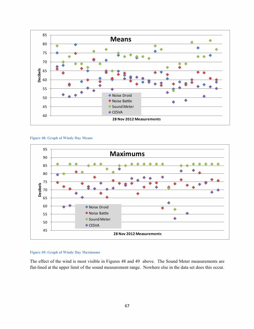
67

40

45

50

55

60

65

70

75

80

85De

cibel

s

28 Nov 2012 Measurements

Means


Figure 48: Graph of Windy Day Means

45

50

55

60

65

70

75

80

85

90

95

Decib

els

28 Nov 2012 Measurements

Maximums


Figure 49: Graph of Windy Day Maximums

The effect of the wind is most visible in Figures 48 and 49 above. The Sound Meter measurements are flat-lined at the upper limit of the sound measurement range. Nowhere else in the data set does this occur.

68

4.4 Discussion of Smart Phone and CESVA Comparisons Noise Battle measurements are closest to Noise Droid measurements, and most of the measurements are in a smaller range. Sound Meter generally records the highest sound measurements, while CESVA generally records the lowest. It is interesting to note these figures in decibels:

• Noise Droid means for the four intervals are 64, 62, 62 and 62 with variances of 34, 30, 28 and 21. • Noise Battle means for the four intervals are 62, 62, 61 and 62 with variances of 19, 19, 16 and 18. • Sound Meter means for the four intervals are 70, 68, 66, and 67 with variances of 38, 38, 31 and 25. • CESVA means for the four intervals are 57, 55, 56 and 56 with variances of 26, 33, 30 and 27. • Noise Battle maximums for the four intervals are 72, 74, 73 and 73 with variances of 23, 31, 21 and

17. • Sound Meter maximums for the four intervals are 82, 81, 79, and 79 with variances of 38, 48, 53 and

49. • CESVA maximums for the four intervals are 70, 68, 70 and 70 with variances of 54, 61, 50 and 67. Spatially, the loudest measurement locations reported by CESVA are on the outer edge of the campus, along the Avenida de Vicente Sos Baynat roadway along the southwest edge of campus. This is due to traffic noise. In the other application reports, these areas as well as seemingly random others inside campus are the loudest. This can be attributed to the smart phone microphone’s higher sensitivity to voices and footsteps passing nearby, which was noted during the fieldwork data collection. That the Noise Droid and Noise Battle measurements are very similar is not surprising. Both these applications recorded for a short time only – eight seconds for Noise Droid and 10 for Noise Battle. Whatever sounds they could capture were very limited in this respect. If no car happened to pass by, then a quiet level was recorded, and vice versa. For Sound Meter and CESVA, however, one car passing by is just part of the story. It could be the main loud event, or one of many. Furthermore, the type of vehicle passing by makes a difference. Motorcycles and buses tend to be louder than passenger vehicles. The segment of noise recorded in a scene could be described as “ambient noise punctuated by transient events,” (Zimmerman 2011) and which snapshot of that segment is recorded determines the picture drawn of that scene.

The differences range from -35 to +35 decibels, with no discernible trends. At this point, differences show that no single number or formula can be applied to the smart phone application measurements to arrive at the professional sound level meter measurements.

Why are the Sound Meter and CESVA recordings so different? Sound Meter recorded for three to four minutes at each location and CESVA for five. The author believes the answer is the calibration of the smart phone itself. During the fieldwork collection, the author observed that the professional equipment was reading a consistently lower decibel level than the smart phone applications. Additionally, the smart phone appeared to be more sensitive to changing sounds such as people walking past or cars driving by. To test this hypothesis, further experiments will be necessary to compare various mobile devices and see how each one records noise levels using the three applications. This experiment is discussed in the next section.

69

4.5 Comparisons of Samsung Mobile Devices Further testing by means of gathering as many as possible models of the Android phones in one place and using each of the three applications to simultaneously measure the noise level at a well-known source such as an outdoor fountain is one way to see how their instrumentation varies. This test was held on Wednesday, February 13, 2013. The phones were placed on the 9 centimeter tall ledge three meters from the fountain on the north side of the first Technology and Experimental Sciences building. Two different Galaxy Y models, a Galaxy SII, a Galaxy Ace and a Galaxy Tablet were tested. Figures 50 and 51 show the results.

50

55

60

65

70

75

80

85

90

95

Galaxy Y a Galaxy Y b Galaxy SII Galaxy Ace Galaxy Tablet

Decib

els

Samsung Mobile Device

Samsung Mobile Device Means

Noise Droid

Noise Battle

Sound Meter

Figure 50: Graph of Samsung Mobile Device Means

Galaxy Y a is consistently about five decibels higher than Galaxy Y b. Galaxy Y b is similar to the Galaxy SII, except for with the Sound Meter. The Galaxy Tablet has the lowest Sound Meter measurement, the Galaxy Ace has the lowest Noise Battle measurement and the Galaxy Y b has the lowest Noise Droid measurement. The Galaxy Y a has the highest average of the means of the three applications, at 77.5 decibels, while the Galaxy Ace and the Galaxy Tablet are tied for the lowest overall average, at 68.6 and 68.8 decibels, respectively. The fact that these measurements, taken in the same space and time, can be so different, shows that the results of crowdsourcing noise data varies between mobile devices.

70

50

55

60

65

70

75

80

85

90

95

Galaxy Y a Galaxy Y b Galaxy SII Galaxy Ace Galaxy Tablet

Decib

els

Samsung Mobile Device

Samsung Mobile Device Maximums

Noise Droid

Noise Battle

Sound Meter

Figure 51: Graph of Samsung Mobile Device Maximums

Again, Galaxy Y a is consistently about five decibels higher than Galaxy Y b. The Galaxy Tablet has the lowest Sound Meter measurement, the Galaxy Ace has the lowest Noise Battle measurement and the Galaxy Y’s are tied for the lowest Noise Droid measurement. The Galaxy SII has the highest average of the maximums of the three applications, at 83.3 decibels, while the Galaxy Y b and the Galaxy Ace are tied for the lowest overall average, at 75.4 and 75.5 decibels, respectively. The fact that these measurements, taken in the same space and time, can be so different, shows that the results of crowdsourcing noise data varies between mobile devices. Note that these measurements were taken at constant noise source: a fountain. Therefore the means and the maximums do not vary as much as the sound measurements taken for the previous work. Variation can be explained by passing voices, footsteps, and cars.

71

4.6 Comparison of GPS Locations to Georeferenced Measurement Locations Another element to consider when evaluating crowdsourced noise data to that collected by professional equipment is the ground location. Figure 52 shows gray circles representing the georeferenced measurement locations. These were verified by the author first using point to point onscreen matching with the ArcGIS Georeferencing tool. Next they were corrected by a combination of “ground-truthing:” and onscreen digitizing. In other words, using personal knowledge (from physically being present during the recordings) that measurements were taken on a particular sidewalk corner or strip, and never in the street or on top of a building, the author corrected the locations by overlaying them on the UJI Smart Campus Street Pavement data and moving them to the proper position. The red dots represent all the locations as recorded by the Noise Battle smart phone application during fieldwork, which were determined by the smart phone’s internal Global Positioning System (GPS).

Figure 52: Map of Georeferenced and GPS Measurement Locations

As Figure 52 shows, the locations recorded by the smart phone’s GPS are variable and several occur far from the actual location and even on top of buildings. When considering the quality of crowdsourced data, it is important to realize that the locations will not necessarily be reliable. At the very least, users of the noise database will have to clean the data by visually inspecting and removing or adjusting points in locations which, for example, fall on top of buildings.

72

5. Results: Which is the best methodology to make a noise map?

5.1 Geostatistical Approach ArcGIS has many geostatistical interpolation tools as well as cross validation tools. After mapping the CESVA First Interval dataset for reference in Figure 53 below and using various data exploration tools such as histograms, quantile-quantile plots and tend analysis, the author used several of these to try to arrive at the best noise map. The first two interpolation tools are like those in the Spatial Analyst Extension, but being in the Geostatistical Analyst Extension, they also have the option of creating a geostatistical layer, or prediction map, which can be used as an input for the Cross Validation tool. It runs the interpolation algorithm as many times as there are input measurement points. Each time, it leaves out one point and uses the rest to predict what that point would be. In this way, a set of predicted measurements can be graphed against the measured points to compare for the interpolation method’s validity. A black trend line is shown on top of the cross validation scatter plots in this section. The closer this trend line is to the 45° line (a one to one ratio), the more valid the method of interpolation is. The blue line is the trend line which matches the dataset comparison. For the other interpolation methods, the cross validation is done manually and does not represent a prediction created by removing each point at a time. These comparisons represent how well the noise field generated actually matches the measurements.

Figure 53: Map CESVA First Interval

There are several types of interpolation methods. Deterministic methods create a surface which actually passes through all of the measurement points. As it makes sense to use this methodology for noise sample points, these tools will be explored first.

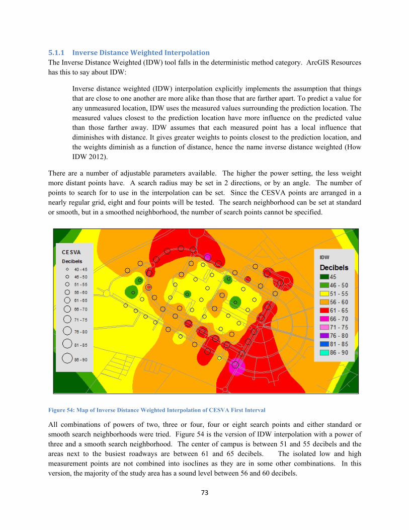
73

5.1.1 Inverse Distance Weighted Interpolation The Inverse Distance Weighted (IDW) tool falls in the deterministic method category. ArcGIS Resources has this to say about IDW:

Inverse distance weighted (IDW) interpolation explicitly implements the assumption that things that are close to one another are more alike than those that are farther apart. To predict a value for any unmeasured location, IDW uses the measured values surrounding the prediction location. The measured values closest to the prediction location have more influence on the predicted value than those farther away. IDW assumes that each measured point has a local influence that diminishes with distance. It gives greater weights to points closest to the prediction location, and the weights diminish as a function of distance, hence the name inverse distance weighted (How IDW 2012).

There are a number of adjustable parameters available. The higher the power setting, the less weight more distant points have. A search radius may be set in 2 directions, or by an angle. The number of points to search for to use in the interpolation can be set. Since the CESVA points are arranged in a nearly regular grid, eight and four points will be tested. The search neighborhood can be set at standard or smooth, but in a smoothed neighborhood, the number of search points cannot be specified.

Figure 54: Map of Inverse Distance Weighted Interpolation of CESVA First Interval

All combinations of powers of two, three or four, four or eight search points and either standard or smooth search neighborhoods were tried. Figure 54 is the version of IDW interpolation with a power of three and a smooth search neighborhood. The center of campus is between 51 and 55 decibels and the areas next to the busiest roadways are between 61 and 65 decibels. The isolated low and high measurement points are not combined into isoclines as they are in some other combinations. In this version, the majority of the study area has a sound level between 56 and 60 decibels.

74

Figure 55: IDW Cross Validation Graph

The cross validation graph in Figure 55 is scattered far less than the smart phone measurements were. This represents the closest IDW came to predicting the measurement points accurately. The trend line is flatter than and intersects the 45° line at just above 55 decibels.

Mean Variance t-StatisticPredicted 56.5 5.8CESVA 56.7 25.7

0.37(0.71)

Table 22: t-Test of IDW Interpolation

Table 22 is the results of the t-Test for this interpolation method. The value of the statistical test used to compare the means is 0.37. The p-value is more than 5%, so the IDW predictions and CESVA measurements are not statistically significantly different.

75

Figure 56: Graph of IDW Interpolation of CESVA First Interval

Figure 56 shows the CESVA measurements plotted with the predictions made by IDW interpolation. Many of them are very close. The differences range from -11.6 to 21 decibels.

76

5.1.2 Radial Based Function Interpolation The other deterministic interpolation method is Radial Basis Function (RBF). There are five different functions available: completely regularized spline, spline with tension, multi-quadratic function, inverse multi-quadratic function and thin plate spline. “RBFs are conceptually similar to fitting a rubber membrane through the measured sample values while minimizing the total curvature of the surface. The basis function you select determines how the rubber membrane will fit between the values” (How RBS 2012).

Figure 57: Map of Radial Based Function Interpolation of CESVA First Interval

Figure 57 shows the results of the multi-quadratic function interpolation. Like areas are combined rather than remaining separated as in the IDW interpolation. Again, most of the campus area is between 51 and 55 decibels, but the majority of the study area is between 61 and 65 decibels. This function results in some areas beyond the noisy roadways being between 66 and 70 decibels.

77

Figure 58: RBF Cross Validation Graph

The graph in Figure 58 shows a tighter fit of points to the trend line, which is centered on the chart. This is the closest RBF came to predicting the measurement points accurately. It is more accurate than the best IDW interpolation, as the trend line is steeper and closer to the 45° line. Again, the intersection is just above 55 decibels.


0.08(0.94)

Table 23: t-Test of RBF Interpolation

Table 23 is the results of the t-Test for this interpolation method. The value of the statistical test used to compare the means is 0.08. The p-value is more than 5%, so the RBF predictions and CESVA measurements are not statistically significantly different.

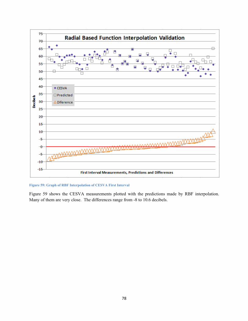
78

Figure 59: Graph of RBF Interpolation of CESVA First Interval

Figure 59 shows the CESVA measurements plotted with the predictions made by RBF interpolation. Many of them are very close. The differences range from -8 to 10.6 decibels.

79

5.1.3 Kriging Interpolation Kriging is not a deterministic method of interpolation, but it is the method used by some of the researchers in the literature reviewed for this thesis as well as the method ReMa uses. Therefore, it is included in this exploration. In the Geostatistical and Spatial Analyst toolsets, various versions of kriging were tested. Kriging methods…

…are based on statistical models that include autocorrelation—that is, the statistical relationships among the measured points. Because of this, geostatistical techniques not only have the capability of producing a prediction surface but also provide some measure of the certainty or accuracy of the predictions. (How Kriging works 2012).

Ordinary kriging with a four point search radius produced the best, most accurate interpolation out of all the other methods.

Figure 60: Map of Kriging Interpolation of CESVA First Interval

Figure 60 is the noise map created by kriging which predicts noise measurements most accurately. The most significant distinction in the results shown here compared with deterministic methods is that the actual measurement points are not represented in the surface. For example, the small areas of 46 to 50 decibels are not visible like on the other maps. Another striking difference is the large area of 46 to 50 decibels predicted in the lower left corner. Otherwise, it is similar with the central campus area at 51 to 55 decibels, the roadway areas at 61 to 65 decibels and areas of 66 to 70 decibels predicted beyond the sample points.

80

Figure 61: Graph o f Kriging Cross Validation

In order to compare the noise map to the geostatististical interpolations, cross validation was calculated by hand using the identify tool at each measurement location to ascertain the noise map predicted value. These were plotted against each other in the same way. As shown in Figure 61, ordinary kriging interpolation produces the most accurate prediction results. The points are closer to the trend line than in any other figure, and the trend line, while not parallel, is closer to the 45° line than any other comparison. Only two points stray from the trend line, and these are closer than the majority of points in other comparisons.


0.16(0.88)

Table 24: t-Test of Kriging Interpolation

Table 24 is the results of the t-Test for this interpolation method. The value of the statistical test used to compare the means is 0.16. The p-value is more than 5%, so the RBF predictions and CESVA measurements are not statistically significantly different.

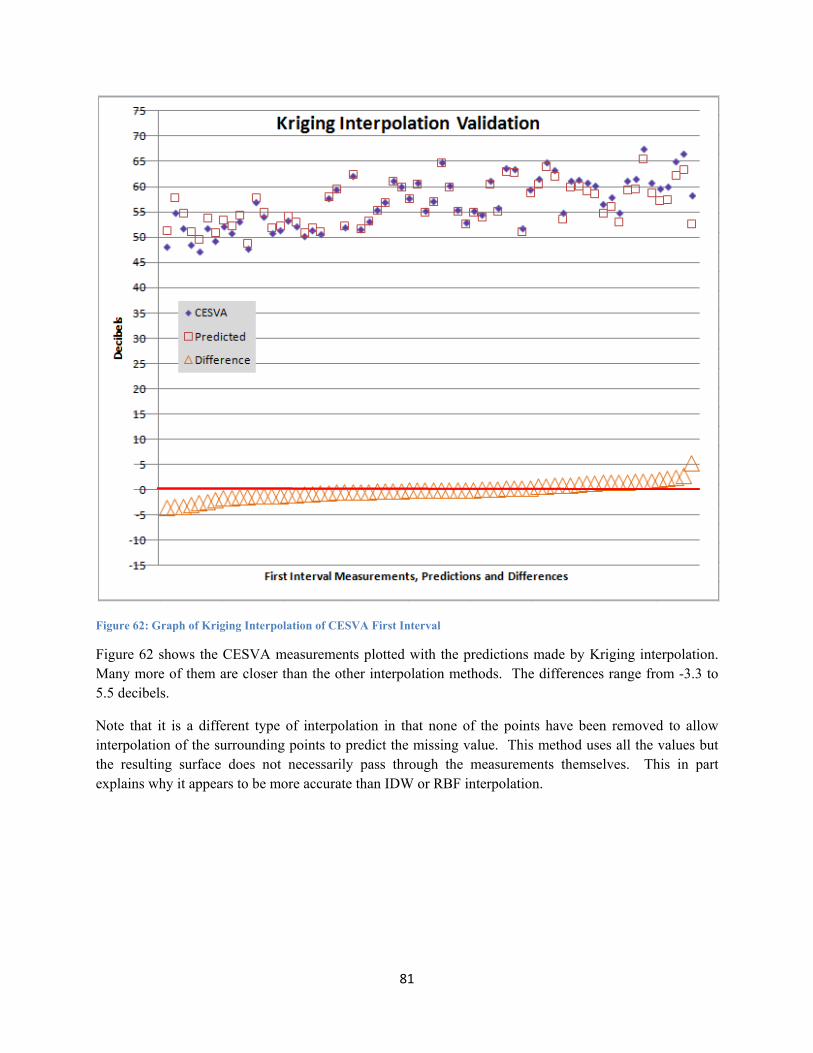
81

Figure 62: Graph of Kriging Interpolation of CESVA First Interval

Figure 62 shows the CESVA measurements plotted with the predictions made by Kriging interpolation. Many more of them are closer than the other interpolation methods. The differences range from -3.3 to 5.5 decibels.

Note that it is a different type of interpolation in that none of the points have been removed to allow interpolation of the surrounding points to predict the missing value. This method uses all the values but the resulting surface does not necessarily pass through the measurements themselves. This in part explains why it appears to be more accurate than IDW or RBF interpolation.

82

5.2 Noise Source Attenuation Approach

5.2.1 Impact Decay Function The ideas for this approach come from the research done by researchers in Brazil mentioned in the literature review. Oliviera et. all define the elements involved in the acoustic model very succinctly:

Sound is a wave phenomenon essentially involving the propagation of mechanical waves in a medium. Sound is produced by sources (the noise emitting elements, having a geometry and properties which vary for each case), modified by obstacles (barriers to the propagation of sound, absorbing it or reflecting it in varying percentages, depending on their nature and their position in the vicinity of sources), and perceived by receivers (the elements which are disturbed by the noise, that is, buildings, installations, and people, or a combination of them) (Oliviera 1999).

They go on to describe two important aspects of acoustic modeling, propagation and combination. In other words, considering the spatial distribution of the attenuation of sound from each source and then combining those effects across the environment. Simply put, the model would need to account for the attenuation of sound for each noise source into the surrounding environment and each source’s attenuation would need to be combined with that of all the other noise sources. Similarly, for a grid of noise measurements, interpolating the values in between would be achieved by combining the attenuation of the value at each known location. This grid of measurements acts as receivers. It will be interesting to compare the map created by noise sources to that created by noise receivers.

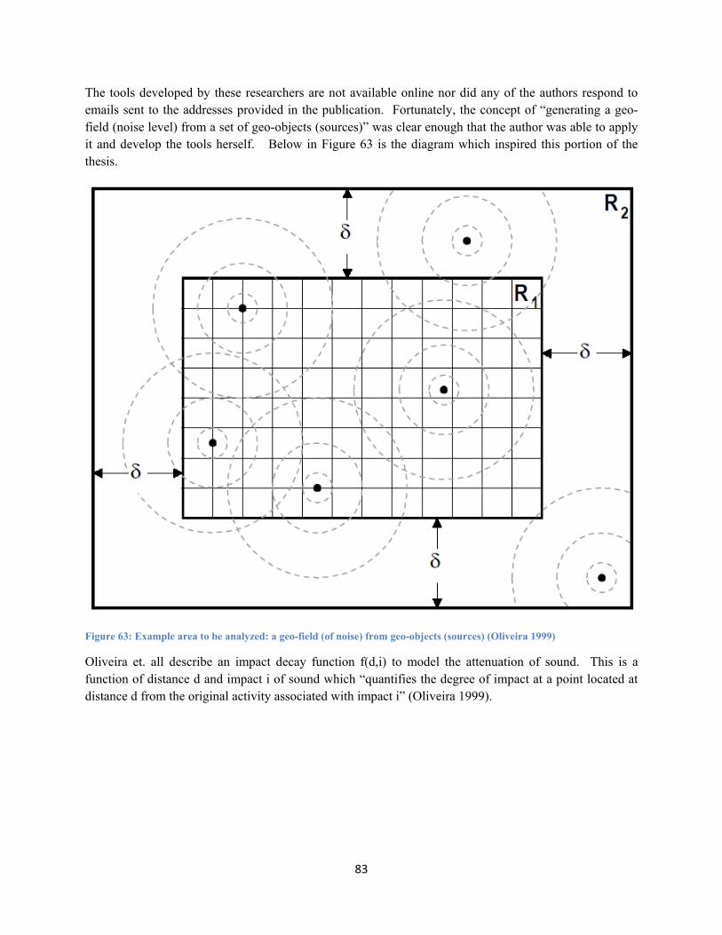
83

The tools developed by these researchers are not available online nor did any of the authors respond to emails sent to the addresses provided in the publication. Fortunately, the concept of “generating a geo-field (noise level) from a set of geo-objects (sources)” was clear enough that the author was able to apply it and develop the tools herself. Below in Figure 63 is the diagram which inspired this portion of the thesis.

Figure 63: Example area to be analyzed: a geo-field (of noise) from geo-objects (sources) (Oliveira 1999)

Oliveira et. all describe an impact decay function f(d,i) to model the attenuation of sound. This is a function of distance d and impact i of sound which “quantifies the degree of impact at a point located at distance d from the original activity associated with impact i” (Oliveira 1999).

84

The first step is to determine the attenuation of sound from each source. Oliveira gives the equation:

SPL1 – SPL2 = 20 log (r1/r2)

to define “the relationship between SPL1 and SPL2 which are the sound pressure levels at distances r1 and r2 from the source” (Oliveira 1999). But this format is not intuitive as the terms are not explicitly defined and therefore are easily misunderstood. According to Peter Mapp, the same equation is written:

dB = 20 log (d1/d2)

where dB is the drop in decibels, d1 is the distance for the unknown decibel level and d2 is the distance at the known decibel level. Therefore, to calculate the attenuation for a given distance from the source, the equation can be written as:

dB1 = dB2 - 20 log (d1/d2)

where dB1 is the unknown decibel level at the distance d1 and dB2 is the original decibel level at the known distance. This is an equation which can be translated into GIS terms, which will be discussed below.

The second step is to combine the SPLs for all the noise sources in the area. Oliveira gives the equation:

SPLt = L1 + 10 log [ 1 + 10( - (L1 - L2)/10) ] dB

where SPLt is the total sound pressure level, L1 is the SPL of one source and L2 id the SPL of a second source (Oliveira 1999). But this is only the total for two sources. The following equation by E. Sengpiel allows the totaling of any number n sources:

LΣ = 10*log10 (10L1/10 + 10L2/10 +…. + 10Ln/10)

where LΣ is the total level and L1, L2,…Ln are the sound pressure levels of the n sources (Sengpiel 2012). This equation, as well, can be translated into GIS terms. This is explained below.

85

5.2.2 Creation of Propagation Tool with ArcGIS Modelbuilder The author decided to use Modelbuilder to apply these rules in the form of the equations explained above in an ArcGIS setting. Each term in the equation must be represented by a raster layer with the correct value(s) for that term. These terms will then be manipulated in the ArcGIS Spatial Analyst Extension Map Algebra tool, the raster calculator. Below in Figure 64 are the steps as defined by the author for creating a noise map in ArcGIS:

86

Figure 64: Propagation Tool Created by Author

87

Step one is to create the raster which represents the decibel value at a noise source. It will be used as the dB2 term in the equation dB1 = dB2 - 20 log (d1/d2). An iterator is used to select each feature in the feature class specified in the model parameter. A separate raster must be created for each feature in each layer of noise sources, each time the value must be set to the decibel level of the desired feature before running the feature to raster tool. The study area feature is simply a polygon drawn around the UJI campus and surrounding areas. Its dimensions, extending beyond the explicit bounding box defined by the extents of the campus, were chosen by the author to attempt to create a more realistic model. Since UJI does not exist in a vacuum, but instead is in the midst of a bustling town full of traffic and just southwest of the large Autopista del Mediterrani, these surrounding noises must surely contribute to the noise on campus. Therefore, to accurately draw a noise map, these surrounding areas must be included in the model. Setting the value of the feature to the decibel level of the source creates an easy-to-manipulate raster for the following calculations. The cell size set at one means that each grid cell in the raster will represent one meter squared on the ground.

Step two is to create the raster which represents the distance at which the decibel level is unknown. It will be used as the d1 term in the equation dB1 = dB2 - 20 log (d1/d2). It also must be run for each feature in each layer of noise sources, the iterator each time selecting the desired feature in a definition query before running the Euclidean distance tool. The output will be a raster grid where the value of every grid cell equals the distance in meters to the noise source.

The cell size must be set at one meter for this step to work properly as an input for the next step. Setting it at two meters will create a raster with even numbers only, which means there is no distance of one. In order for the original decibel level for the measurement point to retain its value in the next step, there must be a distance of one meter to calculate with. When the Euclidean distance is zero or one, during the next step, log(0) returns no data since it is invalid and log (1) returns zero. The zero works perfectly at cell size one, because the area directly around the measurement point retains its decibel value. But at cell size of two meters, there will be no one meter distance, no zero value and therefore the highest decibel level returned in the next step will be approximately six decibels less than the original value (since 20 * log(2)) = 6). (Steps thus far are shown larger in Figure 65 below.)

88

Figure 65: Detail 1 of Propagation Tool

89

Step three is to create the attenuation raster. This step uses the equation dB1 = dB2 - 20 log (d1/d2). Verbally, it states that the decibel level in each grid cell equals the decibel level at the noise source minus twenty times the log of the distance to each grid cell divided by the distance to the noise source at the known decibel level. However, since the final term, the distance to the noise source at the known decibel level is zero, or point blank, there is no need to include it in the equation. In other words, the desired outcome of the equation is the decibel level at every actual distance, not at a distance divided by anything.

Note that removing the d2 term from the formula is the only way to calculate all the distances with the Euclidean Distance raster, but it means that the decay rate is the highest possible. However, when compared to results in Oliveira et al., this seems to be an acceptable result, and the noise map created by it makes the most sense at large scales (showing small areas).

Step four is to remove the negative values created by the previous step. These are inevitable since at some point, the sound attenuates to zero. However, it is also necessary to eliminate values below the ambient sound level for an outdoor environment, because even in the quietest urban place, the lowest limit is forty decibels (Airport 2012). Therefore, with this step, all values below forty are reset to forty.

Step five is simply a division of the attenuated sound levels by ten, so that the values can be used as the exponents in the next step. Map algebra’s raster calculator will only accept either a raster as input for the exponent with an integer for the number to be raised by that exponent, or vice versa. This step ends the set of steps to be performed on each feature of each noise source layer. This completes the first model, called Propagation, shown larger in Figure 66 below.

90

Figure 66: Detail 2 of Propagation Tool

91

5.2.3 Creation of Combination Tool with ArcGIS Modelbuilder The next steps are to combine the final output from the previous calculations together to create a complete noise map. The tool is shown below in Figure 67.

92

Figure 67: Combination Tool Created by Author: (32 points, nine lines and three road sources are the inputs, colored blue)

93

Step six is to combine the outputs from the previous calculations using the equation LΣ=10*log10(10L1/10 + 10L2/10 +…. + 10Ln/10). A separate model called Combination has been created by the author to calculate this final step. Each final output from the Propagation model is used as one exponent in the equation. Maps for each feature type (point, line and polygon) may be created as well as one map with all features of all noise sources. The latter represents the truest noise source map.

94

5.2.4 Noise Source Attenuation Map

Figure 68: Noise Source Attenuation Map Created by Author

The final output, shown in Figure 68, combines all the road, point and line sources into one surface representing the propagation, attenuation and combination of sound from these multiple sources.

95

Figure 69: Noise Source Attenuation Map with CESVA First Interval

Unlike the geostatististical interpolation noise maps, the majority of the map in Figure 69 has a decibel level between 56 and 60. This is because the main noise source influencing the environment is the roadways, with a decibel level of 65. This was partially determined based on the mean of all the intervals for the CESVA dataset along the Avenida de Vicente Sos Baynat roadway along the southwest edge of campus at 63 decibels. Using a lower number for roadways inside the campus, would bring down the campus interpolation and should be explored further.

96

Figure 70: Noise Source Attenuation Cross Validation Graph

In order to compare the noise map to the geostatististical interpolations, cross validation was calculated by hand using the identify tool at each measurement location to ascertain the noise map predicted value. These were plotted against each other in the same way and are shown in Figure 70.

The trend line is flatter than the other interpolation methods, but the points are spread in a similar way to IDW and RBF, in the center of the chart. However, due to the higher decibel levels calculated by using the road traffic noise sources, the trend line intersection with the 45° line is just above 60 decibels.


-5.0(2.85E-06)

Table 25: t-Test of Noise Source Attenuation

Table 25 is the results of the t-Test for this comparison method. The value of the statistical test used to compare the means is -5.0. The p-value is less than 5%, so the Noise Source Attenuation predictions and CESVA measurements are statistically significantly different. Again, adjusting the road traffic decibel levels would be an interesting way to explore the potential accuracy of this prediction method.

97

Figure 71: Graph of Noise Source Attenuation and CESVA First Interval

Figure 71 shows the CESVA measurements plotted with the predictions made by the Noise Source Attenuation. Fewer points are as close to the actual measurements than with the other interpolation methods. The differences range from -11.3 to 6.5 decibels.

Note that it is a different type of comparison, in that none of the points have been removed to allow interpolation of the surrounding points to predict the missing value. Furthermore, it is not interpolation at all, but a geo-field (noise) created by geo-objects (noise sources) (Oliveira 1999). This method uses none of the measurement values, however, the surface created from known noise sources is still very close to the actual sound measurements as recorded by the CESVA.

98

The color of the points are in the same scale as the source map, so large scale details of instances where the decibel levels match are shown in Figure 72 below. Despite the fact that the measurement points were not used to create this surface, many of the predicted values are very close.

Figure 72: Details of Accuracy Prediction by Noise Source Attenuation Map

99

Three points, or 5% of the 66, are predicted to be less than one decibel away from the measurement point. Eleven more are less than two decibels away, totaling 17%. Nine more are less than three decibels away (the slightest change perceptible to humans), now totaling 36%. Eleven more are less than four decibels away, reaching 53%. Eight more are less than five decibels away (a clearly noticeable change), bringing the final total to 61% accuracy rate of a less than 5 decibel discrepancy.

The decibel levels used as inputs for this model were the maximum estimates: point and line sources taken with a smart phone (the Galaxy SII) and road sources estimated based on internet tables of vehicle noise pollution. Therefore, this noise map produced represents the worst case scenario (loud traffic on all the roads, at all times.) Unlike the maps created from interpolating sample noise receiver measurements done at different times of the day, this noise source attenuation map is a general map representing no specific time of day. Actual measurements with a certified, calibrated professional sound level meter, at different intervals of the day (and different days of the week since the campus is less populated on weekends) would have the potential to make richer, more strategic noise source maps.

100

6. Conclusions and Future Work The comparisons of smart phone measurements with the professional sound level measurements revealed that they are not of comparable quality. Each and every ANOVA and t-Test revealed statistically significant differences. This is mostly attributed to the phone’s hardware. Further testing by means of gathering as many as possible models of the Android phones in one place and using each of the three applications to simultaneously measure the noise level at a well-known source, an outdoor fountain in this case, was one way to see how their instrumentation varies. This test revealed very different results. In addition, the phone used to do the fieldwork for this thesis recorded decibel levels consistently five decibels higher than the other model just like it. Otherwise, the measurements seemed to vary randomly, indicating that crowdsourced noise data is subject to variations in mobile devices. Additionally, software allowing users to calibrate the smart phone microphone could be developed and implemented. Human error was controlled in this research, but that is not guaranteed or likely in situations where random citizens are taking sound measurements. A more rigorous quality check and quality assurance system would be needed to control the human error element in the real-life environment. The locations reported from smart phone GPS systems vary widely and may occur in improbable locations, such as on top of buildings. This indicates a necessity for crowdsourced database users to visually inspect point locations and determine how best to handle these erroneous locations.

The geostatistical interpolation tools delivered noise maps which had similar accuracy rates for predicting measurement points according to the cross validation methods used. The best (most accurate) prediction model was indeed the kriging method, as suggested by the literature and by ReMa. The fit of the points in the noise source attenuation noise map was very similar to that of the geostatistical methods, only slightly higher. Future work could be done to improve the noise source attenuation map, such as adjusting the decibel levels for the roadways inside the UJI campus.

After the data collection had already taken place, the author discovered a publication called SPreADGIS, which is an ArcGIS toolset developed specifically for modeling noise in forests (Reed 2009). None of the inputs required had been gathered with the sound measurements, so it was too late to attempt to explore this approach. Future data collection would do well to also gather atmospheric and other types of data so that this well–established toolset can be tested in a university environment.

Finally, the author created something new that had not been done before in GIS. This can be the basis for future improvements. These improvements would incorporate spatial and temporal data including, but not limited to, three-dimensional topography; buildings, street furniture, trees and other barriers along with information about their absorbent and reflective surfaces; atmospheric conditions like wind speed and direction, humidity and air and ground temperature; and a variety of road and traffic information such as start and stop conditions, road surface, traffic density at various times of day and week. However, with the limited data available for the UJI campus at this time and with an eye to creating a simple solution which could be utilized in other municipalities and universities where this data is scarce or lacking, the author succeeded in attaining the goal. Another future project could be to use the professional sound level meter to record actual road traffic noise and use these values for the noise source attenuation map. The author successfully applied sound attenuation equations to create a multiple noise source propagation and combination interpolation toolset in ArcGIS. This has not been done before and the model created can be used for an infinite number of noise sources.

101

The research done by Oliveira et.al. which inspired this portion of the thesis took modeling the acoustic environment several steps further. They integrated the GIS tools in geodatabase for their city in Brazil, which was very rich in the types of information needed to create a real model of the environment:

The prototype was built within “SEAU” (the Portuguese acronym for: Urban Spatial Analysis Environmental System). SEAU is based on a GIS, operating on a large urban geographic database. It enables the access to a very large number of additional details of the urban environment, which can be at times quite helpful in the analysis of the licensing process. The data used include information location and nature of economic activities, street network, land use zones, and several others. The complete geographic database comprises more than 250 object classes (Oliveira 1999).

Once the UJI Smart Campus has grown into a similar resource, integrating the Propagation and Combination tools into it would be a very rewarding exercise and could potentially result in a more strategic noise map than is currently possible.

102

7. Implications Because of the range of human hearing, sound can be considered a subjective thing not easily quantified. The decibel scale is applied to fit the logarithmic-like range, but reality is more complicated than that. Humans have the ability to selectively filter and even “tune out” sounds. Concentration, distraction, level of alertness, fatigue, health and even age can be factors in the way humans perceive sounds, and any of it can change in a matter of seconds. Psychology can be applied to define perceptiveness, but the truth is that the perception of sound is relative from one human being to the next.

For example, try to convince someone that it is quiet. He may be sitting at his desk at work, surrounded by coworkers constantly typing. If he is accustomed to this setting and is having a good day, he may agree. Sitting next to him, a woman just got an email from her boss demanding why a certain deadline has not been met. Suddenly, the roar of typing all around her becomes deafening, and all she can think is, “Why can’t they just be quiet?!” Or, think of a house in the countryside at night. The silence is broken by the howl of a wolf, which is miles and miles away. This sound will barely register on a sound level meter, if at all, but it can be argued that that sound broke the quiet and it could easily be said it was loud.

To try to be objective using instrumentation and human senses, certain conclusions can be found. But the fact that the energy of sound decreases with distance complicates the success of the quantifying. Perhaps a subjectivity scale such as slight, loud, very loud, too loud and unbearable should be submitted along with noise maps in order to paint the whole picture. This could be a way to pair human sensibilities with mathematics.

This thesis is concerns objectifying sounds around the UJI campus. The noise source attenuation map the author created may show sound dropping rapidly with distance, but, on the other hand, it could be difficult to convince a student that a particular sound is not objectionable. Because of the ability of humans to distinguish types of sounds and volume levels, a car horn honking may only register at 51 decibels, but it is likely that it sounds loud to a studying student.

103

8. References Airport Noise Law. Last accessed 2 Jan 2013 http://airportnoiselaw.org/dblevels.html

Arana M, San Martin R, Nagore I, Perez D (2012) Main results of strategic noise maps and action plans in Navarre (Spain). Environ Monit Assess . Arana M, San Martin R, San Martin ML, Aramendia E (2010) Strategic noise map of a major road carried out with two environmental prediction software packages. Environ Monit Assess 163:503-513.

CESVA Acoustic Instruments (2011). SC-20c Sonometro integrador-promediador. (In Spanish)

Comparative Examples of Noise Levels by Industrial Noise Control, Inc. Last accessed 30 Jan 2013. http://www.industrialnoisecontrol.com/comparative-noise-examples.htm

De Muer T, Botteldooren D (2003) Uncertainty in Noise Mapping: Comparing a Probabilistic and a Fuzz Set Approach. T. Bilgi¸c et al. (Eds.): IFSA 2003, LNAI 2715, pp. 229–236, 2003.

Decibel (Loudness) Comparison Chart by Galen Carol Audio. Last accessed 30 Jan 2013. http://www.gcaudio.com/resources/howtos/loudness.html

Directive 2002/49/EC of the European Parliament and of the Council of 25 June relating to the assessment and management of environmental noise (2002).

European Commission Working Group Assessment of Exposure to Noise (WG-AEN). Good Practice Guide for Strategic Noise Mapping and the Production of Associated Data on Noise Exposure, January 2006.

Future Noise Policy, European Commission Green Paper. (1996) Brussels; Commission of the European Communities.

Garcia Marti I, Rodriguez L, Benedito M, Trilles S, Beltran A, Diaz L, Huerta J (2012) Mobile Application for Noise Pollution Monitoring through Gamification Techniques. Lecture Notes in Computer Science, 2012, Volume 7522/2012, Entertainment Computing – ICEC 2012, pp. 562-571, DOI: 10.1007/978-3-642-33542-6_74.

Histograms by ESRI in ArcGIS Resources. Last accessed 31 Jan 2013. http://resources.arcgis.com/es/help/main/10.1/index.html#/na/00310000000p000000/

How Inverse Distance Weighted Interpolation Works by ESRI in ArcGIS Resources. Last accessed 26 Jan 2013 http://resources.arcgis.com/en/help/main/10.1/index.html#/How_inverse_distance_weighted_interpolation_works/00310000002m000000/

How Kriging Works by ESRI in ArcGIS Resources. Last accessed 19 Feb 2013. http://resources.arcgis.com/en/help/main/10.1/index.html#/How_Kriging_works/009z00000076000000/

http://airportnoiselaw.org/dblevels.html�

http://www.industrialnoisecontrol.com/comparative-noise-examples.htm�

http://www.gcaudio.com/resources/howtos/loudness.html�

http://resources.arcgis.com/es/help/main/10.1/index.html#/na/00310000000p000000/�

http://resources.arcgis.com/en/help/main/10.1/index.html#/How_inverse_distance_weighted_interpolation_works/00310000002m000000/�

http://resources.arcgis.com/en/help/main/10.1/index.html#/How_inverse_distance_weighted_interpolation_works/00310000002m000000/�

http://resources.arcgis.com/en/help/main/10.1/index.html#/How_Kriging_works/009z00000076000000/�

104

How Radial Basis Functions Work by ESRI in ArcGIS Resources Last accessed 26 Jan 2013 http://resources.arcgis.com/en/help/main/10.1/index.html#/How_radial_basis_functions_work/00310000002p000000/

Jones, James. Richland Community College. Last accessed 11 January 2013. http://people.richland.edu/james/ictcm/2001/descriptive/helpvariance.html

Kanjo E (2010) NoiseSPY: A Real-Time Mobile Phone Platform for Urban Noise Monitoring and Mapping. Mobile Netw Appl 15:562-574.

Mapp, Peter. Audio System Designer. Klark-Teknik Plc

Michael Minor & Associates. Traffic Noise Background Information. Last accessed 29 Jan 2013. < http://www.drnoise.com/PDF_files/Traffic%20Noise%20Primer.pdf>

Noise Droid by 52 North. Last accessed 30 Jan 2013. https://wiki.52north.org/bin/view/SensorWeb/OpenNoiseMap

Oyedepo O, Saadu A (2010) Evaluation and analysis of noise levels in Ilorin metropolis, Nigeria. Environ Monit Assess (2010) 160:563–577.

Piedade G. Oliveira M, Bauzer Medeiros E, Davis Jr. C (1999) Planning the Acoustic Urban Environment: a GIS-Centered Approach. ACM GIS.

Princeton Online Dictionary. (Last accessed 2 Jan 2013) <wordnetweb.princeton.edu/perl/webwn>

Reed, S.E., J.P. Mann and J.L. Boggs. 2009. SPreAD-GIS: an ArcGIS toolbox for modeling the propagation of engine noise in a wildland setting. Version 1.2. The Wilderness Society, San Francisco, CA.

Sengpiel, E. Forum: Microphone for recording technology and audio engineering. Mixer Institute, University of the Arts Archive. Last accessed 2 Jan 2013. http://www.sengpielaudio.com/calculator-spl.htm

Sound Meter from Google Play. Last accessed 30 Jan 2013. https://play.google.com/store/apps/details?id=kr.sira.sound&hl=en

The Columbia Electronic Encyclopedia, 6th ed. Copyright © 2011, Columbia University Press. <Infoplease.com http://www.infoplease.com/encyclopedia/science/noise-pollution.html#ixzz29bknjqOO>

Wadsworth, Raymond. Basic of Audio and Visual System Design. Longman Higher Education; 1st edition (April 1983)

Weisstein, Eric W. From MathWorld--A Wolfram Web Resource. Last accessed 11 Jan 2013. http://mathworld.wolfram.com

Yilmaz G, Hocanli H (2006) Mapping of Noise by Using GIS in Sanliurfa. Environ Monit Assess 121:103-108.

http://resources.arcgis.com/en/help/main/10.1/index.html#/How_radial_basis_functions_work/00310000002p000000/�

http://resources.arcgis.com/en/help/main/10.1/index.html#/How_radial_basis_functions_work/00310000002p000000/�

http://people.richland.edu/james/ictcm/2001/descriptive/helpvariance.html�

http://www.drnoise.com/PDF_files/Traffic%20Noise%20Primer.pdf�

https://wiki.52north.org/bin/view/SensorWeb/OpenNoiseMap�

http://www.sengpielaudio.com/calculator-spl.htm�

http://www.sengpielaudio.com/calculator-spl.htm�

https://play.google.com/store/apps/details?id=kr.sira.sound&hl=en�

http://www.infoplease.com/encyclopedia/science/noise-pollution.html#ixzz29bknjqOO�

http://mathworld.wolfram.com/�

105

Zimmerman, T and Robson, Christine (2011) Monitoring Residential Noise for Perspective Home Owners and Renters. K. Lyons, J. Hightower, and E.M. Huang (Eds.): Pervasive 2011, LNCS 6696, pp. 34–49, 2011. Springer-Verlag Berlin Heidelberg 2011.

106

9. Appendices

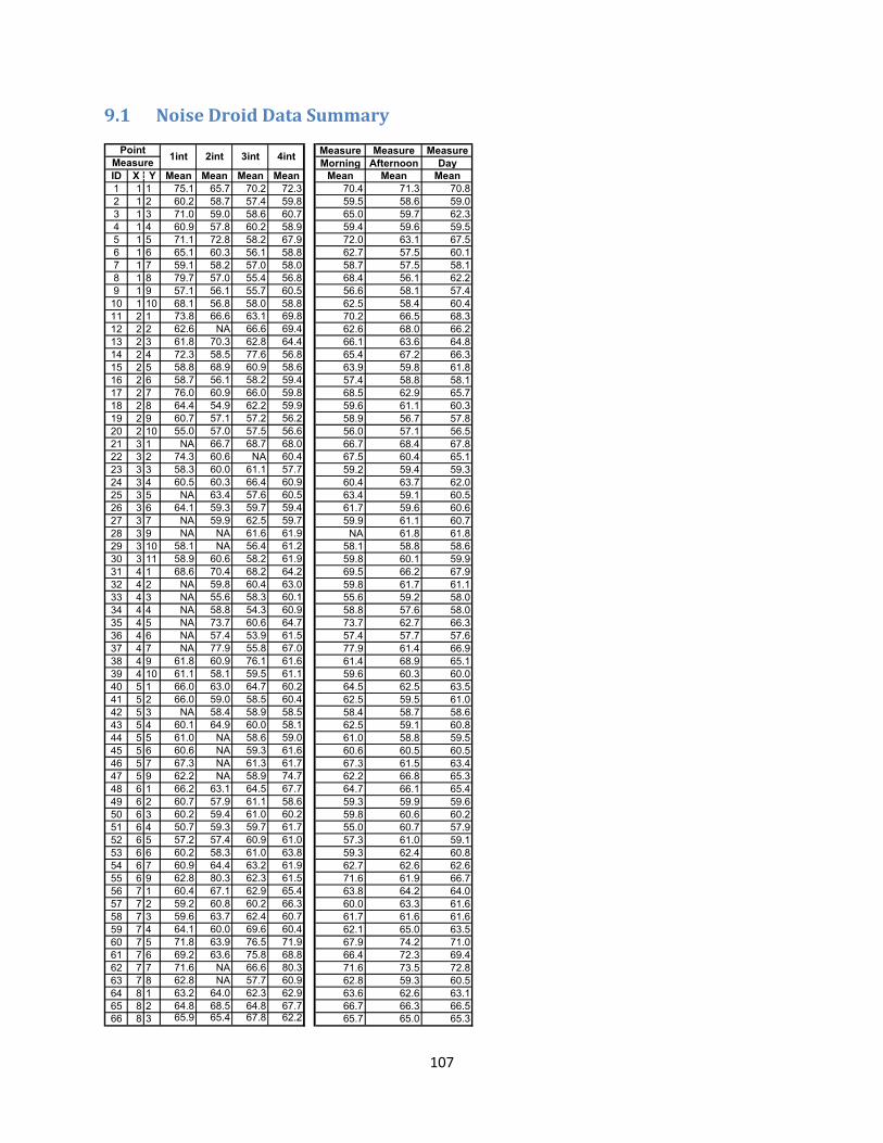
107

9.1 Noise Droid Data Summary

Measure Measure MeasureMorning Afternoon Day

ID X Y Mean Mean Mean Mean Mean Mean Mean1 1 1 75.1 65.7 70.2 72.3 70.4 71.3 70.82 1 2 60.2 58.7 57.4 59.8 59.5 58.6 59.03 1 3 71.0 59.0 58.6 60.7 65.0 59.7 62.34 1 4 60.9 57.8 60.2 58.9 59.4 59.6 59.55 1 5 71.1 72.8 58.2 67.9 72.0 63.1 67.56 1 6 65.1 60.3 56.1 58.8 62.7 57.5 60.17 1 7 59.1 58.2 57.0 58.0 58.7 57.5 58.18 1 8 79.7 57.0 55.4 56.8 68.4 56.1 62.29 1 9 57.1 56.1 55.7 60.5 56.6 58.1 57.410 1 10 68.1 56.8 58.0 58.8 62.5 58.4 60.411 2 1 73.8 66.6 63.1 69.8 70.2 66.5 68.312 2 2 62.6 NA 66.6 69.4 62.6 68.0 66.213 2 3 61.8 70.3 62.8 64.4 66.1 63.6 64.814 2 4 72.3 58.5 77.6 56.8 65.4 67.2 66.315 2 5 58.8 68.9 60.9 58.6 63.9 59.8 61.816 2 6 58.7 56.1 58.2 59.4 57.4 58.8 58.117 2 7 76.0 60.9 66.0 59.8 68.5 62.9 65.718 2 8 64.4 54.9 62.2 59.9 59.6 61.1 60.319 2 9 60.7 57.1 57.2 56.2 58.9 56.7 57.820 2 10 55.0 57.0 57.5 56.6 56.0 57.1 56.521 3 1 NA 66.7 68.7 68.0 66.7 68.4 67.822 3 2 74.3 60.6 NA 60.4 67.5 60.4 65.123 3 3 58.3 60.0 61.1 57.7 59.2 59.4 59.324 3 4 60.5 60.3 66.4 60.9 60.4 63.7 62.025 3 5 NA 63.4 57.6 60.5 63.4 59.1 60.526 3 6 64.1 59.3 59.7 59.4 61.7 59.6 60.627 3 7 NA 59.9 62.5 59.7 59.9 61.1 60.728 3 9 NA NA 61.6 61.9 NA 61.8 61.829 3 10 58.1 NA 56.4 61.2 58.1 58.8 58.630 3 11 58.9 60.6 58.2 61.9 59.8 60.1 59.931 4 1 68.6 70.4 68.2 64.2 69.5 66.2 67.932 4 2 NA 59.8 60.4 63.0 59.8 61.7 61.133 4 3 NA 55.6 58.3 60.1 55.6 59.2 58.034 4 4 NA 58.8 54.3 60.9 58.8 57.6 58.035 4 5 NA 73.7 60.6 64.7 73.7 62.7 66.336 4 6 NA 57.4 53.9 61.5 57.4 57.7 57.637 4 7 NA 77.9 55.8 67.0 77.9 61.4 66.938 4 9 61.8 60.9 76.1 61.6 61.4 68.9 65.139 4 10 61.1 58.1 59.5 61.1 59.6 60.3 60.040 5 1 66.0 63.0 64.7 60.2 64.5 62.5 63.541 5 2 66.0 59.0 58.5 60.4 62.5 59.5 61.042 5 3 NA 58.4 58.9 58.5 58.4 58.7 58.643 5 4 60.1 64.9 60.0 58.1 62.5 59.1 60.844 5 5 61.0 NA 58.6 59.0 61.0 58.8 59.545 5 6 60.6 NA 59.3 61.6 60.6 60.5 60.546 5 7 67.3 NA 61.3 61.7 67.3 61.5 63.447 5 9 62.2 NA 58.9 74.7 62.2 66.8 65.348 6 1 66.2 63.1 64.5 67.7 64.7 66.1 65.449 6 2 60.7 57.9 61.1 58.6 59.3 59.9 59.650 6 3 60.2 59.4 61.0 60.2 59.8 60.6 60.251 6 4 50.7 59.3 59.7 61.7 55.0 60.7 57.952 6 5 57.2 57.4 60.9 61.0 57.3 61.0 59.153 6 6 60.2 58.3 61.0 63.8 59.3 62.4 60.854 6 7 60.9 64.4 63.2 61.9 62.7 62.6 62.655 6 9 62.8 80.3 62.3 61.5 71.6 61.9 66.756 7 1 60.4 67.1 62.9 65.4 63.8 64.2 64.057 7 2 59.2 60.8 60.2 66.3 60.0 63.3 61.658 7 3 59.6 63.7 62.4 60.7 61.7 61.6 61.659 7 4 64.1 60.0 69.6 60.4 62.1 65.0 63.560 7 5 71.8 63.9 76.5 71.9 67.9 74.2 71.061 7 6 69.2 63.6 75.8 68.8 66.4 72.3 69.462 7 7 71.6 NA 66.6 80.3 71.6 73.5 72.863 7 8 62.8 NA 57.7 60.9 62.8 59.3 60.564 8 1 63.2 64.0 62.3 62.9 63.6 62.6 63.165 8 2 64.8 68.5 64.8 67.7 66.7 66.3 66.566 8 3 65.9 65.4 67.8 62.2 65.7 65.0 65.3

3int2int1intPointMeasure 4int

108

9.1.1 Noise Droid First Interval

ID X Y Date Time Min Max Mean Longitude Latitude1 1 1 28-Nov 8:05 75.1 -0.06619 39.990442 1 2 28-Nov 9:21 60.2 -0.0679 39.990623 1 3 28-Nov 9:13 71 -0.06886 39.991024 1 4 28-Nov 9:05 60.9 -0.06996 39.991555 1 5 28-Nov 8:58 71.1 -0.06973 39.993526 1 6 28-Nov 8:50 65.1 -0.07209 39.992447 1 7 28-Nov 8:42 59.1 -0.07313 39.992968 1 8 28-Nov 8:35 79.7 -0.074 39.993589 1 9 28-Nov 8:27 57.1 -0.07478 39.99362

10 1 10 28-Nov 8:20 68.1 -0.07579 39.9940311 2 1 28-Nov 9:31 73.8 -0.06608 39.9908912 2 2 28-Nov 9:39 62.6 -0.06725 39.991513 2 3 28-Nov 9:47 61.8 -0.0681 39.9919814 2 4 28-Nov 9:55 72.3 -0.06931 39.9923915 2 5 28-Nov 10:03 58.8 -0.07124 39.9931416 2 6 28-Nov 10:11 58.7 -0.07159 39.9933217 2 7 28-Nov 10:18 76 -0.07263 39.9937118 2 8 28-Nov 10:26 64.4 -0.0734 39.9945119 2 9 28-Nov 10:33 60.7 -0.07427 39.9944120 2 10 28-Nov 10:41 55 -0.07507 39.994821 3 1 27-Nov 8:16 -0.06597 39.9915222 3 2 27-Nov 8:24 74.3 -0.06676 39.9918623 3 3 27-Nov 8:33 58.3 -0.0678 39.9925324 3 4 27-Nov 8:44 60.5 -0.06953 39.9934525 3 5 27-Nov 8:53 -0.07024 39.9938126 3 6 27-Nov 9:01 64.1 -0.0716 39.9943627 3 7 27-Nov 9:31 -0.07185 39.9944628 3 9 28-Nov 11:07 -0.07373 39.9951229 3 10 28-Nov 10:59 58.1 -0.07455 39.9955330 3 11 28-Nov 10:50 58.9 -0.07547 39.9962231 4 1 27-Nov 10:38 68.6 -0.06512 39.9922532 4 2 27-Nov 10:21 -0.0663 39.9928833 4 3 27-Nov 10:13 -0.06722 39.993334 4 4 27-Nov 10:05 -0.06846 39.9936335 4 5 27-Nov 9:56 -0.06931 39.9943636 4 6 27-Nov 9:48 -0.07065 39.9947137 4 7 27-Nov 9:39 -0.07156 39.9951838 4 9 30-Nov 8:15 61.8 -0.07371 39.996139 4 10 30-Nov 8:05 61.1 -0.07464 39.9965340 5 1 27-Nov 10:46 65.96 -0.06437 39.9932241 5 2 27-Nov 10:55 66 -0.06437 39.9932242 5 3 27-Nov 11:03 -0.06666 39.9941343 5 4 27-Nov 11:12 60.1 -0.06764 39.9945744 5 5 3-Dec 9:47 61 -0.06852 39.9954345 5 6 3-Dec 9:56 60.6 -0.06983 39.9956446 5 7 3-Dec 10:32 67.3 -0.07182 39.9959847 5 9 30-Nov 8:24 62.2 -0.07321 39.9968848 6 1 30-Nov 10:25 66.2 -0.06386 39.993949 6 2 30-Nov 10:35 60.7 -0.06495 39.9944650 6 3 30-Nov 10:45 60.2 -0.06598 39.9951151 6 4 30-Nov 11:00 50.7 -0.06717 39.9958652 6 5 30-Nov 11:09 57.2 -0.06865 39.9958453 6 6 3-Dec 10:08 60.2 -0.06993 39.9954554 6 7 3-Dec 10:25 60.9 -0.07046 39.9960755 6 9 30-Nov 8:33 62.8 -0.07228 39.9973856 7 1 30-Nov 10:16 60.4 -0.06323 39.9947657 7 2 30-Nov 9:57 59.2 -0.06455 39.9951958 7 3 30-Nov 9:29 59.6 -0.06564 39.9957459 7 4 30-Nov 9:20 64.1 -0.0668 39.9960360 7 5 30-Nov 9:11 71.8 -0.06805 39.9966461 7 6 30-Nov 9:02 69.2 -0.06888 39.9967762 7 7 30-Nov 8:52 71.6 -0.07001 39.997563 7 8 30-Nov 8:42 62.8 -0.07127 39.9975464 8 1 30-Nov 10:07 63.2 -0.06283 39.9954165 8 2 30-Nov 9:47 64.8 -0.06407 39.9960566 8 3 30-Nov 9:38 65.9 -0.06491 39.99633

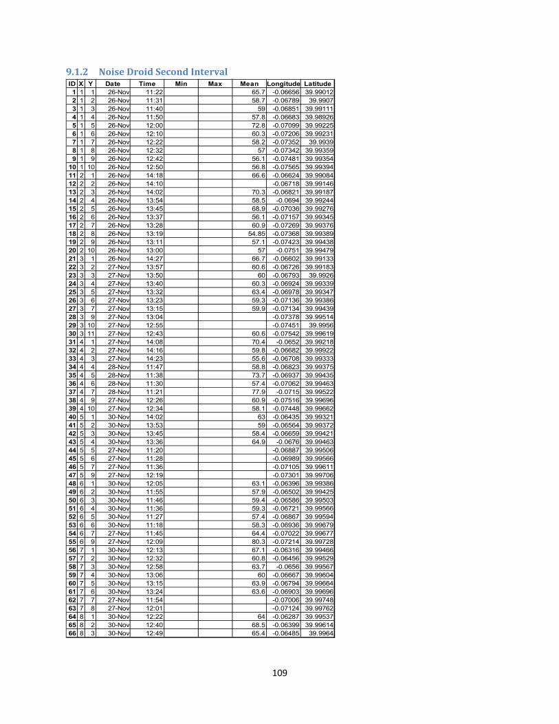
109

9.1.2 Noise Droid Second Interval ID X Y Date Time Min Max Mean Longitude Latitude1 1 1 26-Nov 11:22 65.7 -0.06656 39.990122 1 2 26-Nov 11:31 58.7 -0.06789 39.99073 1 3 26-Nov 11:40 59 -0.06851 39.991114 1 4 26-Nov 11:50 57.8 -0.06683 39.989265 1 5 26-Nov 12:00 72.8 -0.07099 39.992256 1 6 26-Nov 12:10 60.3 -0.07206 39.992317 1 7 26-Nov 12:22 58.2 -0.07352 39.99398 1 8 26-Nov 12:32 57 -0.07342 39.993599 1 9 26-Nov 12:42 56.1 -0.07481 39.99354

10 1 10 26-Nov 12:50 56.8 -0.07565 39.9939411 2 1 26-Nov 14:18 66.6 -0.06624 39.9908412 2 2 26-Nov 14:10 -0.06718 39.9914613 2 3 26-Nov 14:02 70.3 -0.06821 39.9918714 2 4 26-Nov 13:54 58.5 -0.0694 39.9924415 2 5 26-Nov 13:45 68.9 -0.07036 39.9927616 2 6 26-Nov 13:37 56.1 -0.07157 39.9934517 2 7 26-Nov 13:28 60.9 -0.07269 39.9937618 2 8 26-Nov 13:19 54.85 -0.07368 39.9938919 2 9 26-Nov 13:11 57.1 -0.07423 39.9943820 2 10 26-Nov 13:00 57 -0.0751 39.9947921 3 1 26-Nov 14:27 66.7 -0.06602 39.9913322 3 2 27-Nov 13:57 60.6 -0.06726 39.9918323 3 3 27-Nov 13:50 60 -0.06793 39.992624 3 4 27-Nov 13:40 60.3 -0.06924 39.9933925 3 5 27-Nov 13:32 63.4 -0.06978 39.9934726 3 6 27-Nov 13:23 59.3 -0.07136 39.9938627 3 7 27-Nov 13:15 59.9 -0.07134 39.9943928 3 9 27-Nov 13:04 -0.07378 39.9951429 3 10 27-Nov 12:55 -0.07451 39.995630 3 11 27-Nov 12:43 60.6 -0.07542 39.9961931 4 1 27-Nov 14:08 70.4 -0.0652 39.9921832 4 2 27-Nov 14:16 59.8 -0.06682 39.9992233 4 3 27-Nov 14:23 55.6 -0.06708 39.9933334 4 4 28-Nov 11:47 58.8 -0.06823 39.9937535 4 5 28-Nov 11:38 73.7 -0.06937 39.9943536 4 6 28-Nov 11:30 57.4 -0.07062 39.9946337 4 7 28-Nov 11:21 77.9 -0.0715 39.9952238 4 9 27-Nov 12:26 60.9 -0.07516 39.9969639 4 10 27-Nov 12:34 58.1 -0.07448 39.9966240 5 1 30-Nov 14:02 63 -0.06435 39.9932141 5 2 30-Nov 13:53 59 -0.06564 39.9937242 5 3 30-Nov 13:45 58.4 -0.06659 39.9942143 5 4 30-Nov 13:36 64.9 -0.0676 39.9946344 5 5 27-Nov 11:20 -0.06887 39.9950645 5 6 27-Nov 11:28 -0.06989 39.9956646 5 7 27-Nov 11:36 -0.07105 39.9961147 5 9 27-Nov 12:19 -0.07301 39.9970648 6 1 30-Nov 12:05 63.1 -0.06396 39.9938649 6 2 30-Nov 11:55 57.9 -0.06502 39.9942550 6 3 30-Nov 11:46 59.4 -0.06586 39.9950351 6 4 30-Nov 11:36 59.3 -0.06721 39.9956652 6 5 30-Nov 11:27 57.4 -0.06867 39.9959453 6 6 30-Nov 11:18 58.3 -0.06936 39.9967954 6 7 27-Nov 11:45 64.4 -0.07022 39.9967755 6 9 27-Nov 12:09 80.3 -0.07214 39.9972856 7 1 30-Nov 12:13 67.1 -0.06316 39.9946657 7 2 30-Nov 12:32 60.8 -0.06456 39.9952958 7 3 30-Nov 12:58 63.7 -0.0656 39.9956759 7 4 30-Nov 13:06 60 -0.06667 39.9960460 7 5 30-Nov 13:15 63.9 -0.06794 39.9966461 7 6 30-Nov 13:24 63.6 -0.06903 39.9969662 7 7 27-Nov 11:54 -0.07006 39.9974863 7 8 27-Nov 12:01 -0.07124 39.9976264 8 1 30-Nov 12:22 64 -0.06287 39.9953765 8 2 30-Nov 12:40 68.5 -0.06399 39.9961466 8 3 30-Nov 12:49 65.4 -0.06485 39.9964

110

9.1.3 Noise Droid Third Interval ID X Y Date Time Min Max Mean Longitude Latitude1 1 1 27-Nov 16:19 70.2 -0.06666 39.990082 1 2 27-Nov 16:30 57.4 -0.06682 39.989223 1 3 27-Nov 16:38 58.6 -0.06817 39.991264 1 4 27-Nov 16:47 60.2 -0.06682 39.989225 1 5 27-Nov 16:55 58.2 -0.07094 39.992386 1 6 27-Nov 17:04 56.1 -0.07225 39.992417 1 7 27-Nov 17:11 57 -0.07352 39.99398 1 8 27-Nov 17:19 55.4 -0.07379 39.993819 1 9 27-Nov 17:27 55.7 -0.07487 39.99356

10 1 10 27-Nov 17:34 58 -0.07565 39.9939411 2 1 3-Dec 16:01 60.9 73.4 63.1 -0.06629 39.9907312 2 2 3-Dec 15:52 55.7 73.7 66.6 -0.06712 39.9914313 2 3 3-Dec 15:44 58.1 73.7 62.8 -0.0678 39.9915314 2 4 27-Nov 18:39 77.6 -0.06923 39.9923715 2 5 27-Nov 18:31 60.9 -0.07043 39.9928416 2 6 27-Nov 18:17 58.2 -0.07161 39.9933217 2 7 27-Nov 18:09 66 -0.07256 39.9937618 2 8 27-Nov 18:00 62.2 -0.07343 39.9943819 2 9 27-Nov 17:51 57.2 -0.07426 39.9943320 2 10 27-Nov 17:44 57.5 -0.07509 39.9947421 3 1 3-Dec 16:09 63.4 76.9 68.7 -0.06599 39.991422 3 2 26-Nov 15:40 -0.06693 39.9919923 3 3 26-Nov 15:48 61.1 -0.06784 39.9924524 3 4 26-Nov 15:58 66.4 -0.06919 39.9932925 3 5 26-Nov 16:07 57.6 -0.07026 39.9936526 3 6 26-Nov 16:15 59.7 -0.07122 39.9938127 3 7 26-Nov 16:23 62.5 -0.07165 39.9946128 3 9 26-Nov 16:36 61.6 -0.07392 39.9950929 3 10 26-Nov 16:45 56.4 -0.07409 39.9954530 3 11 26-Nov 16:53 58.2 -0.07542 39.9962931 4 1 30-Nov 16:36 68.2 -0.06508 39.9922932 4 2 30-Nov 16:27 60.4 -0.06639 39.9927533 4 3 30-Nov 16:19 58.3 -0.06724 39.9933534 4 4 30-Nov 16:11 54.3 -0.06826 39.9937435 4 5 30-Nov 16:02 60.6 -0.06933 39.9943836 4 6 30-Nov 15:53 53.9 -0.0705 39.9947737 4 7 30-Nov 15:44 55.8 -0.07124 39.9954638 4 9 26-Nov 17:12 76.1 -0.0737 39.9959139 4 10 26-Nov 17:02 59.5 -0.0744 39.9966540 5 1 30-Nov 16:46 64.7 -0.06445 39.9932141 5 2 30-Nov 16:54 58.5 -0.0656 39.9937342 5 3 30-Nov 17:02 58.9 -0.06657 39.9941743 5 4 30-Nov 17:11 60 -0.06758 39.994744 5 5 30-Nov 17:20 58.6 -0.06889 39.9950545 5 6 30-Nov 17:28 59.3 -0.06988 39.9957146 5 7 30-Nov 17:37 61.3 -0.07112 39.9960747 5 9 26-Nov 17:21 58.9 -0.07311 39.9969348 6 1 30-Nov 18:44 64.5 -0.06397 39.9938549 6 2 30-Nov 18:36 61.1 -0.06504 39.9943850 6 3 30-Nov 18:26 61 -0.06597 39.9947551 6 4 30-Nov 18:12 59.7 -0.06723 39.9956652 6 5 30-Nov 18:02 60.9 -0.06862 39.9958653 6 6 30-Nov 17:54 61 -0.06945 39.9966954 6 7 30-Nov 17:45 63.2 -0.07029 39.9965755 6 9 26-Nov 17:31 62.3 -0.0723 39.9974656 7 1 3-Dec 16:22 59 73.9 62.9 -0.06384 39.9944857 7 2 3-Dec 16:47 54.3 73.9 60.2 -0.06447 39.9944358 7 3 26-Nov 18:32 62.4 -0.06562 39.9956459 7 4 26-Nov 18:23 69.6 -0.06682 39.9961960 7 5 26-Nov 18:13 76.5 -0.06798 39.9966361 7 6 26-Nov 17:57 75.8 -0.0691 39.9969362 7 7 26-Nov 17:48 66.6 -0.06986 39.9976163 7 8 26-Nov 17:38 57.7 -0.07104 39.9975664 8 1 3-Dec 16:30 60.5 70.3 62.3 -0.06333 39.9947865 8 2 3-Dec 16:38 62.2 74.2 64.8 -0.0637 39.995666 8 3 26-Nov 18:41 67.8 -0.06488 39.99666

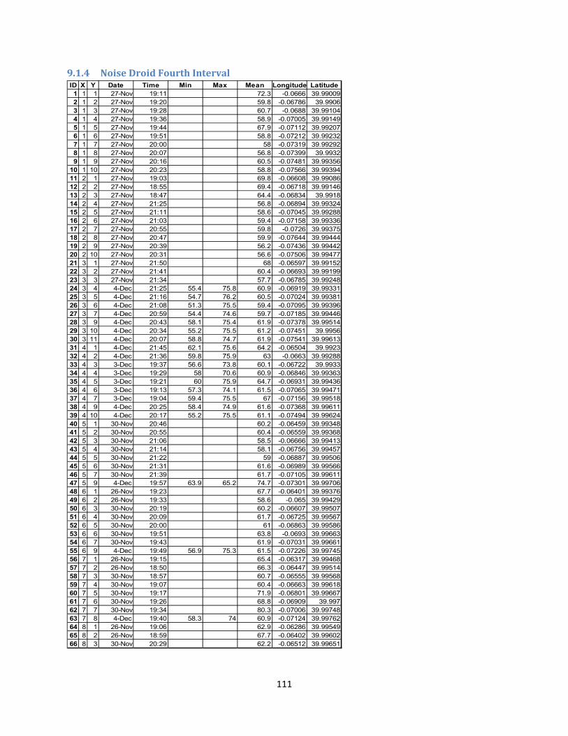
111

9.1.4 Noise Droid Fourth Interval ID X Y Date Time Min Max Mean Longitude Latitude1 1 1 27-Nov 19:11 72.3 -0.0666 39.990092 1 2 27-Nov 19:20 59.8 -0.06786 39.99063 1 3 27-Nov 19:28 60.7 -0.0688 39.991044 1 4 27-Nov 19:36 58.9 -0.07005 39.991495 1 5 27-Nov 19:44 67.9 -0.07112 39.992076 1 6 27-Nov 19:51 58.8 -0.07212 39.992327 1 7 27-Nov 20:00 58 -0.07319 39.992928 1 8 27-Nov 20:07 56.8 -0.07399 39.99329 1 9 27-Nov 20:16 60.5 -0.07481 39.99356

10 1 10 27-Nov 20:23 58.8 -0.07566 39.9939411 2 1 27-Nov 19:03 69.8 -0.06608 39.9908612 2 2 27-Nov 18:55 69.4 -0.06718 39.9914613 2 3 27-Nov 18:47 64.4 -0.06834 39.991814 2 4 27-Nov 21:25 56.8 -0.06894 39.9932415 2 5 27-Nov 21:11 58.6 -0.07045 39.9928816 2 6 27-Nov 21:03 59.4 -0.07158 39.9933617 2 7 27-Nov 20:55 59.8 -0.0726 39.9937518 2 8 27-Nov 20:47 59.9 -0.07644 39.9944419 2 9 27-Nov 20:39 56.2 -0.07436 39.9944220 2 10 27-Nov 20:31 56.6 -0.07506 39.9947721 3 1 27-Nov 21:50 68 -0.06597 39.9915222 3 2 27-Nov 21:41 60.4 -0.06693 39.9919923 3 3 27-Nov 21:34 57.7 -0.06785 39.9924824 3 4 4-Dec 21:25 55.4 75.8 60.9 -0.06919 39.9933125 3 5 4-Dec 21:16 54.7 76.2 60.5 -0.07024 39.9938126 3 6 4-Dec 21:08 51.3 75.5 59.4 -0.07095 39.9939627 3 7 4-Dec 20:59 54.4 74.6 59.7 -0.07185 39.9944628 3 9 4-Dec 20:43 58.1 75.4 61.9 -0.07378 39.9951429 3 10 4-Dec 20:34 55.2 75.5 61.2 -0.07451 39.995630 3 11 4-Dec 20:07 58.8 74.7 61.9 -0.07541 39.9961331 4 1 4-Dec 21:45 62.1 75.6 64.2 -0.06504 39.992332 4 2 4-Dec 21:36 59.8 75.9 63 -0.0663 39.9928833 4 3 3-Dec 19:37 56.6 73.8 60.1 -0.06722 39.993334 4 4 3-Dec 19:29 58 70.6 60.9 -0.06846 39.9936335 4 5 3-Dec 19:21 60 75.9 64.7 -0.06931 39.9943636 4 6 3-Dec 19:13 57.3 74.1 61.5 -0.07065 39.9947137 4 7 3-Dec 19:04 59.4 75.5 67 -0.07156 39.9951838 4 9 4-Dec 20:25 58.4 74.9 61.6 -0.07368 39.9961139 4 10 4-Dec 20:17 55.2 75.5 61.1 -0.07494 39.9962440 5 1 30-Nov 20:46 60.2 -0.06459 39.9934841 5 2 30-Nov 20:55 60.4 -0.06559 39.9936842 5 3 30-Nov 21:06 58.5 -0.06666 39.9941343 5 4 30-Nov 21:14 58.1 -0.06756 39.9945744 5 5 30-Nov 21:22 59 -0.06887 39.9950645 5 6 30-Nov 21:31 61.6 -0.06989 39.9956646 5 7 30-Nov 21:39 61.7 -0.07105 39.9961147 5 9 4-Dec 19:57 63.9 65.2 74.7 -0.07301 39.9970648 6 1 26-Nov 19:23 67.7 -0.06401 39.9937649 6 2 26-Nov 19:33 58.6 -0.065 39.9942950 6 3 30-Nov 20:19 60.2 -0.06607 39.9950751 6 4 30-Nov 20:09 61.7 -0.06725 39.9956752 6 5 30-Nov 20:00 61 -0.06863 39.9958653 6 6 30-Nov 19:51 63.8 -0.0693 39.9966354 6 7 30-Nov 19:43 61.9 -0.07031 39.9966155 6 9 4-Dec 19:49 56.9 75.3 61.5 -0.07226 39.9974556 7 1 26-Nov 19:15 65.4 -0.06317 39.9946857 7 2 26-Nov 18:50 66.3 -0.06447 39.9951458 7 3 30-Nov 18:57 60.7 -0.06555 39.9956859 7 4 30-Nov 19:07 60.4 -0.06663 39.9961860 7 5 30-Nov 19:17 71.9 -0.06801 39.9966761 7 6 30-Nov 19:26 68.8 -0.06909 39.99762 7 7 30-Nov 19:34 80.3 -0.07006 39.9974863 7 8 4-Dec 19:40 58.3 74 60.9 -0.07124 39.9976264 8 1 26-Nov 19:06 62.9 -0.06286 39.9954965 8 2 26-Nov 18:59 67.7 -0.06402 39.9960266 8 3 30-Nov 20:29 62.2 -0.06512 39.99651

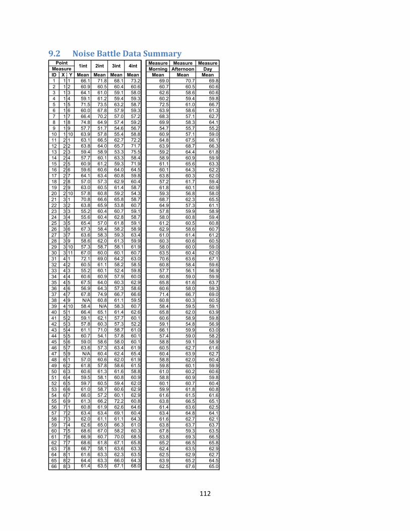
112

9.2 Noise Battle Data Summary Measure Measure MeasureMorning Afternoon Day

ID X Y Mean Mean Mean Mean Mean Mean Mean1 1 1 66.1 71.8 68.1 73.2 69.0 70.7 69.82 1 2 60.9 60.5 60.4 60.6 60.7 60.5 60.63 1 3 64.1 61.0 59.1 58.0 62.6 58.6 60.64 1 4 59.1 61.2 59.4 59.3 60.2 59.4 59.85 1 5 71.5 73.5 63.2 58.7 72.5 61.0 66.76 1 6 60.0 67.8 57.9 59.3 63.9 58.6 61.37 1 7 66.4 70.2 57.0 57.2 68.3 57.1 62.78 1 8 74.8 64.9 57.4 59.2 69.9 58.3 64.19 1 9 57.7 51.7 54.6 56.7 54.7 55.7 55.210 1 10 63.9 57.8 55.4 58.8 60.9 57.1 59.011 2 1 63.1 66.5 62.7 72.2 64.8 67.5 66.112 2 2 63.8 64.0 65.7 71.7 63.9 68.7 66.313 2 3 59.4 58.9 53.3 75.5 59.2 64.4 61.814 2 4 57.7 60.1 63.3 58.4 58.9 60.9 59.915 2 5 60.9 61.2 59.3 71.9 61.1 65.6 63.316 2 6 59.6 60.6 64.0 64.5 60.1 64.3 62.217 2 7 64.1 63.4 60.8 59.8 63.8 60.3 62.018 2 8 57.0 57.3 62.9 60.4 57.2 61.7 59.419 2 9 63.0 60.5 61.4 58.7 61.8 60.1 60.920 2 10 57.8 60.8 59.2 54.3 59.3 56.8 58.021 3 1 70.8 66.6 65.8 58.7 68.7 62.3 65.522 3 2 63.8 65.9 53.8 60.7 64.9 57.3 61.123 3 3 55.2 60.4 60.7 59.1 57.8 59.9 58.924 3 4 55.6 60.4 62.8 58.7 58.0 60.8 59.425 3 5 65.4 57.0 61.8 59.1 61.2 60.5 60.826 3 6 67.3 58.4 58.2 58.9 62.9 58.6 60.727 3 7 63.6 58.3 59.3 63.4 61.0 61.4 61.228 3 9 58.6 62.0 61.3 59.9 60.3 60.6 60.529 3 10 57.3 58.7 58.1 61.9 58.0 60.0 59.030 3 11 67.0 60.0 60.1 60.7 63.5 60.4 62.031 4 1 72.1 69.0 64.2 63.0 70.6 63.6 67.132 4 2 60.5 61.1 58.2 58.5 60.8 58.4 59.633 4 3 55.2 60.1 52.4 59.8 57.7 56.1 56.934 4 4 60.6 60.9 57.9 60.0 60.8 59.0 59.935 4 5 67.5 64.0 60.3 62.9 65.8 61.6 63.736 4 6 56.9 64.3 57.3 58.6 60.6 58.0 59.337 4 7 67.8 74.9 66.7 66.6 71.4 66.7 69.038 4 9 N/A 60.8 61.1 59.5 60.8 60.3 60.539 4 10 58.4 N/A 58.3 60.7 58.4 59.5 59.140 5 1 66.4 65.1 61.4 62.6 65.8 62.0 63.941 5 2 59.1 62.1 57.7 60.1 60.6 58.9 59.842 5 3 57.8 60.3 57.3 52.2 59.1 54.8 56.943 5 4 61.1 71.0 58.7 61.0 66.1 59.9 63.044 5 5 60.7 54.1 57.8 60.1 57.4 59.0 58.245 5 6 59.0 58.6 58.0 60.1 58.8 59.1 58.946 5 7 63.6 57.3 63.4 61.9 60.5 62.7 61.647 5 9 N/A 60.4 62.4 65.4 60.4 63.9 62.748 6 1 57.0 60.6 62.0 61.9 58.8 62.0 60.449 6 2 61.8 57.8 58.6 61.5 59.8 60.1 59.950 6 3 60.6 61.3 61.6 58.8 61.0 60.2 60.651 6 4 59.5 58.1 60.8 60.9 58.8 60.9 59.852 6 5 59.7 60.5 59.4 62.0 60.1 60.7 60.453 6 6 61.0 58.7 60.6 62.9 59.9 61.8 60.854 6 7 66.0 57.2 60.1 62.9 61.6 61.5 61.655 6 9 61.3 66.2 72.2 60.8 63.8 66.5 65.156 7 1 60.8 61.9 62.6 64.6 61.4 63.6 62.557 7 2 63.4 63.4 69.1 60.4 63.4 64.8 64.158 7 3 62.0 61.1 61.1 64.3 61.6 62.7 62.159 7 4 62.6 65.0 66.3 61.0 63.8 63.7 63.760 7 5 68.6 67.0 58.2 60.3 67.8 59.3 63.561 7 6 66.9 60.7 70.0 68.5 63.8 69.3 66.562 7 7 68.6 61.8 67.1 65.8 65.2 66.5 65.863 7 8 66.7 58.1 63.6 63.3 62.4 63.5 62.964 8 1 61.6 63.3 62.3 63.5 62.5 62.9 62.765 8 2 64.4 63.3 66.0 64.3 63.9 65.2 64.566 8 3 61.4 63.5 67.1 68.0 62.5 67.6 65.0


113

9.2.1 Noise Battle First Interval ID X Y Date Time Min Max Mean Longitude Latitude1 1 1 28-Nov 8:05 74.6 66.1 -0.06651 39.990232 1 2 28-Nov 9:21 75.9 60.9 -0.06792 39.99073 1 3 28-Nov 9:13 65.5 64.1 -0.06883 39.991074 1 4 28-Nov 9:05 68 59.1 -0.06995 39.991615 1 5 28-Nov 8:58 77.9 71.5 -0.07103 39.991976 1 6 28-Nov 8:50 72.1 60 -0.07223 39.992447 1 7 28-Nov 8:42 74 66.48 1 8 28-Nov 8:35 81.2 74.89 1 9 28-Nov 8:27 70.7 57.7

10 1 10 28-Nov 8:20 72.12 63.911 2 1 28-Nov 9:31 74.1 63.1 -0.06614 39.9908412 2 2 28-Nov 9:39 73.7 63.8 -0.0672 39.9914113 2 3 28-Nov 9:47 74.1 59.4 -0.06823 39.9919214 2 4 28-Nov 9:55 67.8 57.7 -0.06935 39.9923415 2 5 28-Nov 10:03 71.8 60.9 -0.07031 39.9926916 2 6 28-Nov 10:11 74.1 59.6 -0.07157 39.9933617 2 7 28-Nov 10:18 74.4 64.1 -0.07258 39.9937618 2 8 28-Nov 10:26 58.9 5719 2 9 28-Nov 10:33 71.7 6320 2 10 28-Nov 10:41 73.8 57.821 3 1 27-Nov 8:16 76.9 70.8 -0.06591 39.991622 3 2 27-Nov 8:24 68.9 63.8 -0.06695 39.9919323 3 3 27-Nov 8:33 58.1 55.2 -0.06791 39.9925324 3 4 27-Nov 8:44 58.3 55.625 3 5 27-Nov 8:53 73.5 65.4 -0.07034 39.9936226 3 6 27-Nov 9:01 72.8 67.3 -0.07125 39.9936927 3 7 27-Nov 9:31 76.5 63.6 -0.0721 39.9941328 3 9 28-Nov 11:07 71.6 58.629 3 10 28-Nov 10:59 73 57.330 3 11 28-Nov 10:50 76.3 6731 4 1 27-Nov 10:38 76.6 72.1 -0.06505 39.9923632 4 2 27-Nov 10:21 73.6 60.5 -0.06626 39.9928433 4 3 27-Nov 10:13 67.3 55.2 -0.06713 39.9933434 4 4 27-Nov 10:05 68 60.6 -0.06823 39.9937135 4 5 27-Nov 9:56 74.7 67.5 -0.06923 39.9943136 4 6 27-Nov 9:48 71.9 56.9 -0.07056 39.9946837 4 7 27-Nov 9:39 75.1 67.8 -0.07165 39.9952138 4 9 30-Nov 8:1539 4 10 30-Nov 8:05 59.3 58.440 5 1 27-Nov 10:46 74.9 66.4 -0.06451 39.9932341 5 2 27-Nov 10:55 74.2 59.1 -0.06563 39.9936742 5 3 27-Nov 11:03 73.5 57.8 -0.0664 39.9942443 5 4 27-Nov 11:12 72.6 61.1 -0.06801 39.9955944 5 5 3-Dec 9:47 72.2 60.7 -0.06863 39.9946845 5 6 3-Dec 9:56 73.8 59 -0.06792 39.9911746 5 7 3-Dec 10:32 73.3 63.6 -0.06792 39.9911747 5 9 30-Nov 8:2448 6 1 30-Nov 10:25 58.1 57 -0.0638 39.9938749 6 2 30-Nov 10:35 76.7 61.8 -0.06498 39.9944250 6 3 30-Nov 10:45 76 60.6 -0.06599 39.9950951 6 4 30-Nov 11:00 76.1 59.5 -0.06773 39.9951152 6 5 30-Nov 11:09 76.6 59.7 -0.06824 39.9958553 6 6 3-Dec 10:08 76.4 61 -0.06962 39.9956954 6 7 3-Dec 10:25 70.6 66 -0.06744 39.9982955 6 9 30-Nov 8:33 73.3 61.356 7 1 30-Nov 10:16 74.4 60.8 -0.06323 39.9948957 7 2 30-Nov 9:57 72.1 63.4 -0.0645 39.995158 7 3 30-Nov 9:29 72.7 62 -0.06562 39.9957159 7 4 30-Nov 9:20 72.4 62.6 -0.06694 39.9959260 7 5 30-Nov 9:11 74.2 68.6 -0.06804 39.9966561 7 6 30-Nov 9:02 74.1 66.9 -0.06902 39.9970762 7 7 30-Nov 8:52 76.2 68.6 -0.07002 39.9975763 7 8 30-Nov 8:42 73.1 66.7 -0.0707 39.9960264 8 1 30-Nov 10:07 74.4 61.6 -0.06279 39.9954865 8 2 30-Nov 9:47 72.6 64.4 -0.06405 39.9960866 8 3 30-Nov 9:38 74.2 61.4 -0.06477 39.99644

114

9.2.2 Noise Battle Second Interval ID X Y Date Time Min Max Mean Longitude Latitude1 1 1 26-Nov 11:22 76.5 71.8 -0.06636 39.990442 1 2 26-Nov 11:31 76 60.5 -0.06774 39.990493 1 3 26-Nov 11:40 76.2 61 -0.06896 39.991124 1 4 26-Nov 11:50 76.8 61.2 -0.06683 39.989265 1 5 26-Nov 12:00 77.4 73.5 -0.07107 39.992046 1 6 26-Nov 12:10 69.9 67.8 -0.06683 39.989267 1 7 26-Nov 12:22 81.3 70.2 -0.06842 39.993378 1 8 26-Nov 12:32 50.1 64.9 -0.06855 39.993459 1 9 26-Nov 12:42 52.2 51.69

10 1 10 26-Nov 12:50 74.2 57.811 2 1 26-Nov 14:18 75.7 66.5 -0.06623 39.9909312 2 2 26-Nov 14:10 72 64 -0.06686 39.9917313 2 3 26-Nov 14:02 73.4 58.9 -0.06825 39.9919514 2 4 26-Nov 13:54 72.9 60.115 2 5 26-Nov 13:45 73.2 61.2 -0.07042 39.99316 2 6 26-Nov 13:37 76.9 60.6 -0.07164 39.9933717 2 7 26-Nov 13:28 77 63.4 -0.07245 39.9935818 2 8 26-Nov 13:19 72.6 57.319 2 9 26-Nov 13:11 77.1 60.520 2 10 26-Nov 13:00 76.8 60.821 3 1 26-Nov 14:27 74.3 66.6 -0.06533 39.9913822 3 2 27-Nov 13:57 75 65.9 -0.06726 39.9918723 3 3 27-Nov 13:50 76.1 60.4 -0.06783 39.9924824 3 4 27-Nov 13:40 73.6 60.4 -0.0693 39.9933825 3 5 27-Nov 13:32 66.3 57 -0.07017 39.9937426 3 6 27-Nov 13:23 75 58.4 -0.07155 39.993727 3 7 27-Nov 13:15 74.6 58.3 -0.07172 39.9943928 3 9 27-Nov 13:04 76.5 6229 3 10 27-Nov 12:55 61.8 58.730 3 11 27-Nov 12:43 76.7 6031 4 1 27-Nov 14:08 76 69 -0.06503 39.9922732 4 2 27-Nov 14:16 76.2 61.1 -0.06676 39.9929133 4 3 27-Nov 14:23 75.5 60.1 -0.06719 39.9933634 4 4 28-Nov 11:47 75.8 60.9 -0.06825 39.9937635 4 5 28-Nov 11:38 76.4 64 -0.06938 39.9943836 4 6 28-Nov 11:30 74.7 64.3 -0.07056 39.9946837 4 7 28-Nov 11:21 80.6 74.9 -0.07153 39.9952838 4 9 27-Nov 12:26 74.9 60.839 4 10 27-Nov 12:3440 5 1 30-Nov 14:02 76.7 65.1 -0.06418 39.993441 5 2 30-Nov 13:53 74.1 62.1 -0.06601 39.993742 5 3 30-Nov 13:45 76.4 60.3 -0.06653 39.9941543 5 4 30-Nov 13:36 77.9 71 -0.06757 39.994644 5 5 27-Nov 11:20 55.3 54.1 -0.06888 39.9950445 5 6 27-Nov 11:28 74.8 58.6 -0.06987 39.9957246 5 7 27-Nov 11:36 70.4 57.3 -0.07166 39.9963247 5 9 27-Nov 12:19 76.5 60.448 6 1 30-Nov 12:05 74.1 60.6 -0.06387 39.9938149 6 2 30-Nov 11:55 73.8 57.8 -0.06522 39.9943150 6 3 30-Nov 11:46 77.2 61.3 -0.06557 39.9948551 6 4 30-Nov 11:36 73.7 58.1 -0.06719 39.9956452 6 5 30-Nov 11:27 70.7 60.5 -0.06863 39.9958853 6 6 30-Nov 11:18 74.3 58.7 -0.06892 39.9954354 6 7 27-Nov 11:45 73.1 57.2 -0.07083 39.9977955 6 9 27-Nov 12:09 73.9 66.2 -0.07217 39.9974356 7 1 30-Nov 12:13 74.3 61.9 -0.0635 39.9949457 7 2 30-Nov 12:32 76.8 63.4 -0.06459 39.9953458 7 3 30-Nov 12:58 73.9 61.1 -0.0656 39.9956859 7 4 30-Nov 13:06 75.5 65 -0.06682 39.9959760 7 5 30-Nov 13:15 76.4 6761 7 6 30-Nov 13:24 76 60.7 -0.06902 39.9970162 7 7 27-Nov 11:54 72.5 61.8 -0.07014 39.9974163 7 8 27-Nov 12:01 68.5 58.1 -0.07097 39.9967264 8 1 30-Nov 12:22 72.5 63.3 -0.0628 39.9949465 8 2 30-Nov 12:40 76.1 63.3 -0.06382 39.9960466 8 3 30-Nov 12:49 76.9 63.5 -0.06483 39.99648

115

9.2.3 Noise Battle Third Interval ID X Y Date Time Min Max Mean Longitude Latitude1 1 1 27-Nov 16:19 72.2 68.12 1 2 27-Nov 16:30 76.2 60.4 -0.0677 39.990753 1 3 27-Nov 16:38 72.7 59.1 -0.06876 39.991244 1 4 27-Nov 16:47 71.4 59.4 -0.07001 39.991515 1 5 27-Nov 16:55 68.4 63.2 -0.07111 39.992076 1 6 27-Nov 17:04 72.2 57.9 -0.07196 39.99257 1 7 27-Nov 17:11 72.5 578 1 8 27-Nov 17:19 71.8 57.49 1 9 27-Nov 17:27 69.1 54.6

10 1 10 27-Nov 17:34 70.3 55.411 2 1 3-Dec 16:01 72.9 62.7 -0.06669 39.9917612 2 2 3-Dec 15:52 76.9 65.7 -0.06684 39.991813 2 3 3-Dec 15:44 54.7 53.3 -0.06809 39.9912114 2 4 27-Nov 18:39 73.1 63.3 -0.06931 39.9923615 2 5 27-Nov 18:31 73.5 59.3 -0.07043 39.9928716 2 6 27-Nov 18:17 73.7 64 -0.07159 39.9932917 2 7 27-Nov 18:09 72.7 60.8 -0.07256 39.9937418 2 8 27-Nov 18:00 75.1 62.919 2 9 27-Nov 17:51 73.2 61.420 2 10 27-Nov 17:44 74.2 59.221 3 1 3-Dec 16:09 75.6 65.8 -0.066 39.9914222 3 2 26-Nov 15:40 54.9 53.8 -0.06738 39.9916823 3 3 26-Nov 15:48 76.9 60.7 -0.06784 39.9924524 3 4 26-Nov 15:58 76.5 62.8 -0.06923 39.9932725 3 5 26-Nov 16:07 77.2 61.8 -0.0702 39.993726 3 6 26-Nov 16:15 73.2 58.2 -0.07128 39.9937827 3 7 26-Nov 16:23 75 59.3 -0.07187 39.9943528 3 9 26-Nov 16:36 75.4 61.329 3 10 26-Nov 16:45 73.9 58.130 3 11 26-Nov 16:53 74.4 60.131 4 1 30-Nov 16:36 74 64.2 -0.06507 39.9923132 4 2 30-Nov 16:27 72 58.2 -0.06647 39.9927833 4 3 30-Nov 16:19 54.3 52.4 -0.0679 39.9931634 4 4 30-Nov 16:11 74.1 57.9 -0.06833 39.9936235 4 5 30-Nov 16:02 73.6 60.3 -0.06933 39.9943836 4 6 30-Nov 15:53 73.1 57.3 -0.07073 39.9946237 4 7 30-Nov 15:44 72 66.7 -0.06814 39.9906938 4 9 26-Nov 17:12 76.8 61.139 4 10 26-Nov 17:02 70.7 58.340 5 1 30-Nov 16:46 74.5 61.4 -0.06445 39.9932141 5 2 30-Nov 16:54 73.6 57.7 -0.0656 39.9937442 5 3 30-Nov 17:02 73.8 57.3 -0.06655 39.9941843 5 4 30-Nov 17:11 74 58.7 -0.06763 39.9946344 5 5 30-Nov 17:20 73.8 57.8 -0.0689 39.9950645 5 6 30-Nov 17:28 74 58 -0.06986 39.9957246 5 7 30-Nov 17:37 73.2 63.4 -0.07114 39.9960847 5 9 26-Nov 17:21 77.3 62.448 6 1 30-Nov 18:44 74.4 62 -0.06394 39.9938549 6 2 30-Nov 18:36 70 58.6 -0.06508 39.9943550 6 3 30-Nov 18:26 73.5 61.6 -0.06643 39.994951 6 4 30-Nov 18:12 76.3 60.8 -0.06696 39.9957752 6 5 30-Nov 18:02 73.3 59.4 -0.06863 39.995953 6 6 30-Nov 17:54 73.7 60.6 -0.06946 39.996754 6 7 30-Nov 17:45 74.3 60.1 -0.07029 39.9965755 6 9 26-Nov 17:31 79.9 72.2 -0.07104 39.9977156 7 1 3-Dec 16:22 76.5 62.6 -0.06809 39.9912157 7 2 3-Dec 16:47 74.2 69.1 -0.06481 39.9948658 7 3 26-Nov 18:32 76.5 61.1 -0.06575 39.9955259 7 4 26-Nov 18:23 74.7 66.3 -0.0667 39.9961660 7 5 26-Nov 18:13 74.1 58.2 -0.06682 39.9892461 7 6 26-Nov 17:57 76.7 70 -0.06903 39.9969262 7 7 26-Nov 17:48 74.1 67.1 -0.06995 39.9974363 7 8 26-Nov 17:38 76.8 63.6 -0.07118 39.997864 8 1 3-Dec 16:30 74.2 62.3 -0.06318 39.9949865 8 2 3-Dec 16:38 76.9 66 -0.06352 39.9955466 8 3 26-Nov 18:41 71.6 67.1 -0.06503 39.99656

116

9.2.4 Noise Battle Fourth Interval ID X Y Date Time Min Max Mean Longitude Latitude1 1 1 27-Nov 19:11 76.5 73.2 -0.06663 39.990142 1 2 27-Nov 19:20 73.6 60.6 -0.06783 39.990623 1 3 27-Nov 19:28 68.6 58 -0.06884 39.991054 1 4 27-Nov 19:36 71.9 59.3 -0.07002 39.991565 1 5 27-Nov 19:44 72.5 58.7 -0.07112 39.992036 1 6 27-Nov 19:51 70.8 59.3 -0.07204 39.992467 1 7 27-Nov 20:00 67.3 57.28 1 8 27-Nov 20:07 73.6 59.29 1 9 27-Nov 20:16 68.1 56.7

10 1 10 27-Nov 20:23 74.5 58.811 2 1 27-Nov 19:03 76.1 72.2 -0.0661 39.9908512 2 2 27-Nov 18:55 78.1 71.7 -0.06723 39.9914413 2 3 27-Nov 18:47 82.3 75.5 -0.06823 39.991914 2 4 27-Nov 21:25 73.6 58.4 -0.06937 39.9923115 2 5 27-Nov 21:11 76.4 71.9 -0.07044 39.9928216 2 6 27-Nov 21:03 75.5 64.5 -0.07161 39.9933317 2 7 27-Nov 20:55 71.6 59.8 -0.0726 39.9937418 2 8 27-Nov 20:47 73.9 60.419 2 9 27-Nov 20:39 73.6 58.720 2 10 27-Nov 20:31 65.5 54.321 3 1 27-Nov 21:50 74.2 58.7 -0.06556 39.9917122 3 2 27-Nov 21:41 76.2 60.7 -0.06687 39.9920723 3 3 27-Nov 21:34 69.8 59.1 -0.06784 39.9924424 3 4 4-Dec 21:25 74 58.7 -0.06911 39.9933725 3 5 4-Dec 21:16 73.7 59.1 -0.07027 39.9937826 3 6 4-Dec 21:08 74.3 58.9 -0.06806 39.9912127 3 7 4-Dec 20:59 77.4 63.4 -0.07176 39.9945228 3 9 4-Dec 20:43 74.4 59.929 3 10 4-Dec 20:34 74.4 61.930 3 11 4-Dec 20:07 73.7 60.731 4 1 4-Dec 21:45 74 63 -0.06508 39.992332 4 2 4-Dec 21:36 60.3 58.5 -0.0662 39.9927333 4 3 3-Dec 19:37 74.5 59.8 -0.06733 39.9933734 4 4 3-Dec 19:29 73.5 60 -0.06877 39.9934335 4 5 3-Dec 19:21 74.4 62.9 -0.06945 39.9944236 4 6 3-Dec 19:13 74.2 58.6 -0.06809 39.9912137 4 7 3-Dec 19:04 71.5 66.6 -0.07167 39.9948738 4 9 4-Dec 20:25 73.7 59.539 4 10 4-Dec 20:17 74.4 60.740 5 1 30-Nov 20:46 77.2 62.6 -0.06482 39.9936441 5 2 30-Nov 20:55 73.3 60.1 -0.06562 39.9936342 5 3 30-Nov 21:06 53.3 52.2 -0.06663 39.9940743 5 4 30-Nov 21:14 72 61 -0.0676 39.9945944 5 5 30-Nov 21:22 73.4 60.1 -0.06888 39.9950745 5 6 30-Nov 21:31 73 60.1 -0.06989 39.9956646 5 7 30-Nov 21:39 74.3 61.9 -0.07104 39.9961247 5 9 4-Dec 19:57 74.5 65.4 -0.07072 39.9975348 6 1 26-Nov 19:23 76.5 61.9 -0.06382 39.9937749 6 2 26-Nov 19:33 77.1 61.5 -0.06502 39.9943450 6 3 30-Nov 20:19 73.1 58.8 -0.06605 39.9950151 6 4 30-Nov 20:09 73.8 60.9 -0.06718 39.9956852 6 5 30-Nov 20:00 74.3 62 -0.06863 39.9958653 6 6 30-Nov 19:51 73.7 62.9 -0.06935 39.9966354 6 7 30-Nov 19:43 68.7 62.9 -0.0703 39.996655 6 9 4-Dec 19:49 74.4 60.8 -0.07068 39.9974556 7 1 26-Nov 19:15 73.2 64.6 -0.06335 39.9948457 7 2 26-Nov 18:50 76.1 60.4 -0.06454 39.995258 7 3 30-Nov 18:57 77.5 64.3 -0.06555 39.995759 7 4 30-Nov 19:07 76.1 61 -0.06678 39.9960860 7 5 30-Nov 19:17 63.3 60.3 -0.06605 39.9966861 7 6 30-Nov 19:26 73.9 68.5 -0.0691 39.9969862 7 7 30-Nov 19:34 74.1 65.8 -0.07006 39.9974863 7 8 4-Dec 19:40 75.2 63.3 -0.07102 39.9974864 8 1 26-Nov 19:06 75.4 63.5 -0.06276 39.9954365 8 2 26-Nov 18:59 75.9 64.3 -0.06379 39.9961166 8 3 30-Nov 20:29 74.1 68 -0.06469 39.9961

117

9.3 Sound Meter Data Summary Measure Measure MeasureMorning Afternoon Day

ID X Y Mean Mean Mean Mean Mean Mean Mean1 1 1 79.0 77.0 78.0 78.0 78.0 78.0 78.02 1 2 65.0 62.0 69.0 63.0 63.5 66.0 64.83 1 3 77.0 63.0 60.0 63.0 70.0 61.5 65.84 1 4 69.0 65.0 73.0 66.0 67.0 69.5 68.35 1 5 76.0 80.0 61.0 62.0 78.0 61.5 69.86 1 6 67.0 75.0 66.0 77.0 71.0 71.5 71.37 1 7 69.0 66.0 61.0 70.0 67.5 65.5 66.58 1 8 69.0 60.0 61.0 60.0 64.5 60.5 62.59 1 9 73.0 54.0 66.0 63.0 63.5 64.5 64.010 1 10 70.0 66.0 58.0 59.0 68.0 58.5 63.311 2 1 75.0 75.0 68.0 79.0 75.0 73.5 74.312 2 2 73.0 72.0 71.0 74.0 72.5 72.5 72.513 2 3 74.0 75.0 67.0 76.0 74.5 71.5 73.014 2 4 73.0 74.0 75.0 71.0 73.5 73.0 73.315 2 5 73.0 70.0 75.0 68.0 71.5 71.5 71.516 2 6 72.0 65.0 70.0 72.0 68.5 71.0 69.817 2 7 79.0 65.0 74.0 66.0 72.0 70.0 71.018 2 8 77.0 62.0 74.0 73.0 69.5 73.5 71.519 2 9 67.0 54.0 60.0 62.0 60.5 61.0 60.820 2 10 54.0 59.0 59.0 58.0 56.5 58.5 57.521 3 1 78.0 74.0 71.0 71.0 76.0 71.0 73.522 3 2 68.0 65.0 61.0 63.0 66.5 62.0 64.323 3 3 69.0 64.0 67.0 61.0 66.5 64.0 65.324 3 4 72.0 61.0 66.0 61.0 66.5 63.5 65.025 3 5 73.0 64.0 64.0 60.0 68.5 62.0 65.326 3 6 70.0 61.0 61.0 59.0 65.5 60.0 62.827 3 7 82.0 58.0 64.0 61.0 70.0 62.5 66.328 3 9 81.0 69.0 68.0 69.0 75.0 68.5 71.829 3 10 69.0 65.0 57.0 60.0 67.0 58.5 62.830 3 11 69.0 64.0 61.0 62.0 66.5 61.5 64.031 4 1 73.0 74.0 72.0 68.0 73.5 70.0 71.832 4 2 63.0 66.0 66.0 62.0 64.5 64.0 64.333 4 3 59.0 63.0 60.0 66.0 61.0 63.0 62.034 4 4 73.0 77.0 63.0 70.0 75.0 66.5 70.835 4 5 70.0 82.0 63.0 71.0 76.0 67.0 71.536 4 6 58.0 73.0 69.0 64.0 65.5 66.5 66.037 4 7 74.0 73.0 65.0 69.0 73.5 67.0 70.338 4 9 72.0 69.0 73.0 66.0 70.5 69.5 70.039 4 10 67.0 64.0 62.0 67.0 65.5 64.5 65.040 5 1 78.0 71.0 74.0 70.0 74.5 72.0 73.341 5 2 64.0 65.0 58.0 72.0 64.5 65.0 64.842 5 3 54.0 70.0 56.0 63.0 62.0 59.5 60.843 5 4 73.0 71.0 65.0 67.0 72.0 66.0 69.044 5 5 67.0 68.0 56.0 65.0 67.5 60.5 64.045 5 6 62.0 57.0 58.0 66.0 59.5 62.0 60.846 5 7 66.0 64.0 71.0 73.0 65.0 72.0 68.547 5 9 74.0 72.0 68.0 67.0 73.0 67.5 70.348 6 1 72.0 71.0 67.0 69.0 71.5 68.0 69.849 6 2 66.0 75.0 61.0 59.0 70.5 60.0 65.350 6 3 62.0 60.0 63.0 60.0 61.0 61.5 61.351 6 4 62.0 59.0 72.0 63.0 60.5 67.5 64.052 6 5 59.0 63.0 66.0 66.0 61.0 66.0 63.553 6 6 64.0 68.0 64.0 66.0 66.0 65.0 65.554 6 7 65.0 66.0 67.0 69.0 65.5 68.0 66.855 6 9 76.0 79.0 74.0 69.0 77.5 71.5 74.556 7 1 66.0 71.0 64.0 71.0 68.5 67.5 68.057 7 2 58.0 69.0 71.0 70.0 63.5 70.5 67.058 7 3 68.0 69.0 64.0 65.0 68.5 64.5 66.559 7 4 69.0 69.0 75.0 70.0 69.0 72.5 70.860 7 5 73.0 73.0 73.0 71.0 73.0 72.0 72.561 7 6 76.0 76.0 73.0 70.0 76.0 71.5 73.862 7 7 75.0 67.0 70.0 71.0 71.0 70.5 70.863 7 8 75.0 72.0 65.0 73.0 73.5 69.0 71.364 8 1 68.0 68.0 66.0 67.0 68.0 66.5 67.365 8 2 69.0 67.0 68.0 72.0 68.0 70.0 69.066 8 3 69.0 68.0 73.0 69.0 68.5 71.0 69.8


118

9.3.1 Sound Meter First Interval ID X Y Date Time Min Max Mean1 1 1 28-Nov 8:05 69 86 792 1 2 28-Nov 9:21 61 81 653 1 3 28-Nov 9:13 67 83 774 1 4 28-Nov 9:05 60 86 695 1 5 28-Nov 8:58 60 86 766 1 6 28-Nov 8:50 60 85 677 1 7 28-Nov 8:42 59 81 698 1 8 28-Nov 8:35 56 86 699 1 9 28-Nov 8:27 56 86 73

10 1 10 28-Nov 8:20 59 80 7011 2 1 28-Nov 9:31 65 85 7512 2 2 28-Nov 9:39 58 85 7313 2 3 28-Nov 9:47 56 86 7414 2 4 28-Nov 9:55 54 86 7315 2 5 28-Nov 10:03 54 86 7316 2 6 28-Nov 10:11 54 86 7217 2 7 28-Nov 10:18 60 86 7918 2 8 28-Nov 10:26 60 86 7719 2 9 28-Nov 10:33 53 71 6720 2 10 28-Nov 10:41 52 58 5421 3 1 27-Nov 8:16 60 86 7822 3 2 27-Nov 8:24 60 82 6823 3 3 27-Nov 8:33 56 86 6924 3 4 27-Nov 8:44 58 86 7225 3 5 27-Nov 8:53 57 86 7326 3 6 27-Nov 9:01 57 86 7027 3 7 27-Nov 9:31 60 86 8228 3 9 28-Nov 11:07 57 86 8129 3 10 28-Nov 10:59 54 85 6930 3 11 28-Nov 10:50 57 85 6931 4 1 27-Nov 10:38 57 83 7332 4 2 27-Nov 10:21 56 74 6333 4 3 27-Nov 10:13 55 70 5934 4 4 27-Nov 10:05 60 85 7335 4 5 27-Nov 9:56 60 86 7036 4 6 27-Nov 9:48 53 71 5837 4 7 27-Nov 9:39 56 86 7438 4 9 30-Nov 8:15 60 86 7239 4 10 30-Nov 8:05 58 74 6740 5 1 27-Nov 10:46 61 84 7841 5 2 27-Nov 10:55 56 76 6442 5 3 27-Nov 11:03 52 61 5443 5 4 27-Nov 11:12 56 86 7344 5 5 3-Dec 9:47 56 78 6745 5 6 3-Dec 9:56 57 77 6246 5 7 3-Dec 10:32 55 82 6647 5 9 30-Nov 8:24 63 86 7448 6 1 30-Nov 10:25 54 86 7249 6 2 30-Nov 10:35 52 84 6650 6 3 30-Nov 10:45 54 71 6251 6 4 30-Nov 11:00 51 80 6252 6 5 30-Nov 11:09 48 73 5953 6 6 3-Dec 10:08 56 81 6454 6 7 3-Dec 10:25 58 77 6555 6 9 30-Nov 8:33 65 85 7656 7 1 30-Nov 10:16 57 79 6657 7 2 30-Nov 9:57 55 80 5858 7 3 30-Nov 9:29 55 81 6859 7 4 30-Nov 9:20 63 82 6960 7 5 30-Nov 9:11 59 86 7361 7 6 30-Nov 9:02 62 86 7662 7 7 30-Nov 8:52 68 85 7563 7 8 30-Nov 8:42 63 86 7564 8 1 30-Nov 10:07 61 75 6865 8 2 30-Nov 9:47 59 76 6966 8 3 30-Nov 9:38 60 76 69

119

9.3.2 Sound Meter Second Interval ID X Y Date Time Min Max Mean1 1 1 26-Nov 11:22 59 86 772 1 2 26-Nov 11:31 56 81 623 1 3 26-Nov 11:40 57 80 634 1 4 26-Nov 11:50 56 83 655 1 5 26-Nov 12:00 59 86 806 1 6 26-Nov 12:10 0:00 85 757 1 7 26-Nov 12:22 55 84 668 1 8 26-Nov 12:32 56 63 609 1 9 26-Nov 12:42 52 56 54

10 1 10 26-Nov 12:50 52 81 6611 2 1 26-Nov 14:18 61 86 7512 2 2 26-Nov 14:10 56 85 7213 2 3 26-Nov 14:02 55 86 7514 2 4 26-Nov 13:54 53 86 7415 2 5 26-Nov 13:45 52 85 7016 2 6 26-Nov 13:37 50 80 6517 2 7 26-Nov 13:28 54 76 6518 2 8 26-Nov 13:19 51 80 6219 2 9 26-Nov 13:11 52 58 5420 2 10 26-Nov 13:00 52 74 5921 3 1 26-Nov 14:27 57 86 7422 3 2 27-Nov 13:57 54 77 6523 3 3 27-Nov 13:50 55 83 6424 3 4 27-Nov 13:40 48 75 6125 3 5 27-Nov 13:32 51 85 6426 3 6 27-Nov 13:23 46 78 6127 3 7 27-Nov 13:15 50 71 5828 3 9 27-Nov 13:04 52 86 6929 3 10 27-Nov 12:55 53 85 6530 3 11 27-Nov 12:43 53 82 6431 4 1 27-Nov 14:08 58 84 7432 4 2 27-Nov 14:16 56 78 6633 4 3 27-Nov 14:23 53 78 6334 4 4 28-Nov 11:47 57 86 7735 4 5 28-Nov 11:38 63 86 8236 4 6 28-Nov 11:30 54 86 7337 4 7 28-Nov 11:21 58 86 7338 4 9 27-Nov 12:26 56 86 6939 4 10 27-Nov 12:34 52 84 6440 5 1 30-Nov 14:02 57 86 7141 5 2 30-Nov 13:53 56 81 6542 5 3 30-Nov 13:45 51 86 7043 5 4 30-Nov 13:36 52 86 7144 5 5 27-Nov 11:20 57 85 6845 5 6 27-Nov 11:28 50 74 5746 5 7 27-Nov 11:36 54 75 6447 5 9 27-Nov 12:19 57 86 7248 6 1 30-Nov 12:05 57 86 7149 6 2 30-Nov 11:55 52 59 7550 6 3 30-Nov 11:46 51 79 6051 6 4 30-Nov 11:36 47 75 5952 6 5 30-Nov 11:27 48 81 6353 6 6 30-Nov 11:18 50 81 6854 6 7 27-Nov 11:45 50 85 6655 6 9 27-Nov 12:09 57 86 7956 7 1 30-Nov 12:13 58 86 7157 7 2 30-Nov 12:32 54 83 6958 7 3 30-Nov 12:58 54 84 6959 7 4 30-Nov 13:06 58 83 6960 7 5 30-Nov 13:15 52 86 7361 7 6 30-Nov 13:24 53 86 7662 7 7 27-Nov 11:54 58 78 6763 7 8 27-Nov 12:01 54 86 7264 8 1 30-Nov 12:22 62 77 6865 8 2 30-Nov 12:40 55 77 6766 8 3 30-Nov 12:49 59 76 68

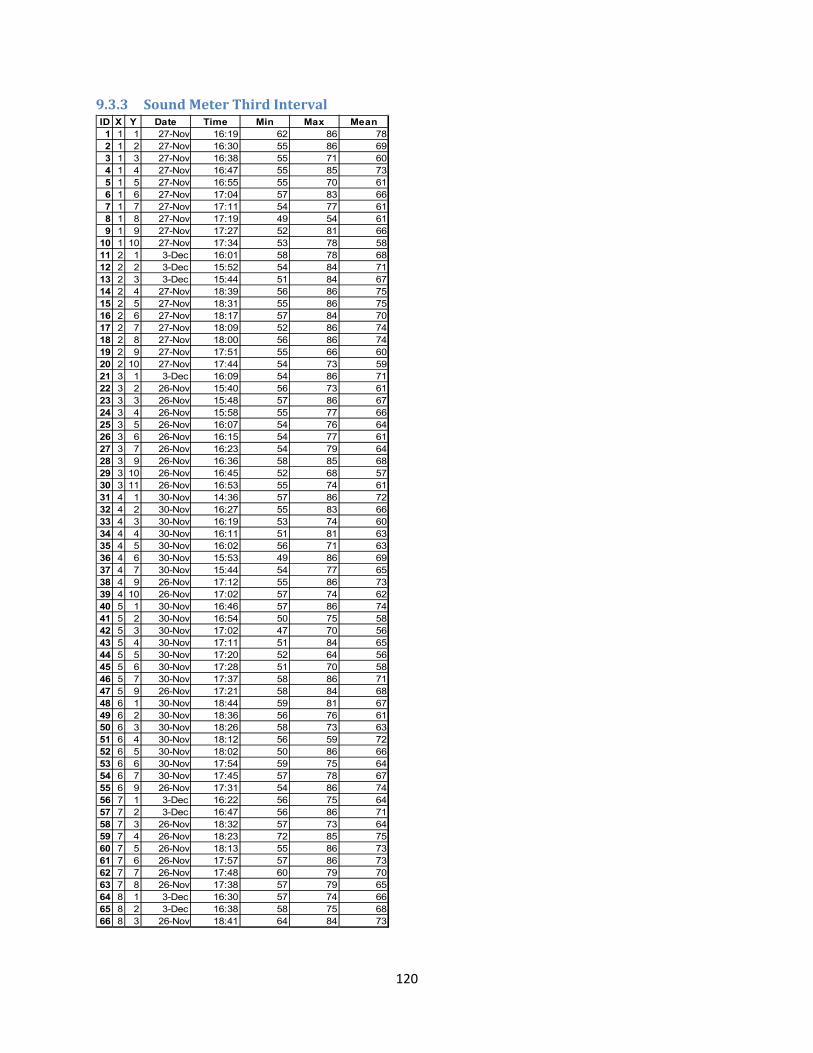
120

9.3.3 Sound Meter Third Interval ID X Y Date Time Min Max Mean1 1 1 27-Nov 16:19 62 86 782 1 2 27-Nov 16:30 55 86 693 1 3 27-Nov 16:38 55 71 604 1 4 27-Nov 16:47 55 85 735 1 5 27-Nov 16:55 55 70 616 1 6 27-Nov 17:04 57 83 667 1 7 27-Nov 17:11 54 77 618 1 8 27-Nov 17:19 49 54 619 1 9 27-Nov 17:27 52 81 66

10 1 10 27-Nov 17:34 53 78 5811 2 1 3-Dec 16:01 58 78 6812 2 2 3-Dec 15:52 54 84 7113 2 3 3-Dec 15:44 51 84 6714 2 4 27-Nov 18:39 56 86 7515 2 5 27-Nov 18:31 55 86 7516 2 6 27-Nov 18:17 57 84 7017 2 7 27-Nov 18:09 52 86 7418 2 8 27-Nov 18:00 56 86 7419 2 9 27-Nov 17:51 55 66 6020 2 10 27-Nov 17:44 54 73 5921 3 1 3-Dec 16:09 54 86 7122 3 2 26-Nov 15:40 56 73 6123 3 3 26-Nov 15:48 57 86 6724 3 4 26-Nov 15:58 55 77 6625 3 5 26-Nov 16:07 54 76 6426 3 6 26-Nov 16:15 54 77 6127 3 7 26-Nov 16:23 54 79 6428 3 9 26-Nov 16:36 58 85 6829 3 10 26-Nov 16:45 52 68 5730 3 11 26-Nov 16:53 55 74 6131 4 1 30-Nov 14:36 57 86 7232 4 2 30-Nov 16:27 55 83 6633 4 3 30-Nov 16:19 53 74 6034 4 4 30-Nov 16:11 51 81 6335 4 5 30-Nov 16:02 56 71 6336 4 6 30-Nov 15:53 49 86 6937 4 7 30-Nov 15:44 54 77 6538 4 9 26-Nov 17:12 55 86 7339 4 10 26-Nov 17:02 57 74 6240 5 1 30-Nov 16:46 57 86 7441 5 2 30-Nov 16:54 50 75 5842 5 3 30-Nov 17:02 47 70 5643 5 4 30-Nov 17:11 51 84 6544 5 5 30-Nov 17:20 52 64 5645 5 6 30-Nov 17:28 51 70 5846 5 7 30-Nov 17:37 58 86 7147 5 9 26-Nov 17:21 58 84 6848 6 1 30-Nov 18:44 59 81 6749 6 2 30-Nov 18:36 56 76 6150 6 3 30-Nov 18:26 58 73 6351 6 4 30-Nov 18:12 56 59 7252 6 5 30-Nov 18:02 50 86 6653 6 6 30-Nov 17:54 59 75 6454 6 7 30-Nov 17:45 57 78 6755 6 9 26-Nov 17:31 54 86 7456 7 1 3-Dec 16:22 56 75 6457 7 2 3-Dec 16:47 56 86 7158 7 3 26-Nov 18:32 57 73 6459 7 4 26-Nov 18:23 72 85 7560 7 5 26-Nov 18:13 55 86 7361 7 6 26-Nov 17:57 57 86 7362 7 7 26-Nov 17:48 60 79 7063 7 8 26-Nov 17:38 57 79 6564 8 1 3-Dec 16:30 57 74 6665 8 2 3-Dec 16:38 58 75 6866 8 3 26-Nov 18:41 64 84 73

121

9.3.4 Sound Meter Fourth Interval ID X Y Date Time Min Max Mean

1 1 1 27-Nov 19:11 66 86 782 1 2 27-Nov 19:20 58 78 633 1 3 27-Nov 19:28 60 73 634 1 4 27-Nov 19:36 58 84 665 1 5 27-Nov 19:44 57 74 626 1 6 27-Nov 19:51 55 86 777 1 7 27-Nov 20:00 56 86 708 1 8 27-Nov 20:07 55 68 609 1 9 27-Nov 20:16 54 76 63

10 1 10 27-Nov 20:23 56 62 5911 2 1 27-Nov 19:03 68 86 7912 2 2 27-Nov 18:55 58 86 7413 2 3 27-Nov 18:47 56 86 7614 2 4 27-Nov 21:25 53 86 7115 2 5 27-Nov 21:11 53 86 6816 2 6 27-Nov 21:03 59 86 7217 2 7 27-Nov 20:55 58 76 6618 2 8 27-Nov 20:47 61 86 7319 2 9 27-Nov 20:39 56 70 6220 2 10 27-Nov 20:31 56 60 5821 3 1 27-Nov 21:50 53 86 7122 3 2 27-Nov 21:41 59 72 6323 3 3 27-Nov 21:34 57 73 6124 3 4 4-Dec 21:25 54 70 6125 3 5 4-Dec 21:16 55 73 6026 3 6 4-Dec 21:08 52 69 5927 3 7 4-Dec 20:59 53 78 6128 3 9 4-Dec 20:43 56 86 6929 3 10 4-Dec 20:34 55 66 6030 3 11 4-Dec 20:07 54 72 6231 4 1 4-Dec 21:45 56 80 6832 4 2 4-Dec 21:36 56 68 6233 4 3 3-Dec 19:37 58 75 6634 4 4 3-Dec 19:29 55 86 7035 4 5 3-Dec 19:21 63 78 7136 4 6 3-Dec 19:13 53 77 6437 4 7 3-Dec 19:04 58 81 6938 4 9 4-Dec 20:25 53 81 6639 4 10 4-Dec 20:17 54 77 6740 5 1 30-Nov 20:46 58 85 7041 5 2 30-Nov 20:55 55 68 7242 5 3 30-Nov 21:06 53 77 6343 5 4 30-Nov 21:14 52 84 6744 5 5 30-Nov 21:22 54 80 6545 5 6 30-Nov 21:31 59 78 6646 5 7 30-Nov 21:39 59 86 7347 5 9 4-Dec 19:57 59 84 6748 6 1 26-Nov 19:23 57 79 6949 6 2 26-Nov 19:33 54 69 5950 6 3 30-Nov 20:19 56 70 6051 6 4 30-Nov 20:09 59 71 6352 6 5 30-Nov 20:00 60 85 6653 6 6 30-Nov 19:51 62 73 6654 6 7 30-Nov 19:43 62 78 6955 6 9 4-Dec 19:49 60 86 6956 7 1 26-Nov 19:15 62 85 7157 7 2 26-Nov 18:50 56 85 7058 7 3 30-Nov 18:57 58 81 6559 7 4 30-Nov 19:07 58 85 7060 7 5 30-Nov 19:17 58 86 7161 7 6 30-Nov 19:26 60 86 7062 7 7 30-Nov 19:34 63 81 7163 7 8 4-Dec 19:40 63 86 7364 8 1 26-Nov 19:06 58 73 6765 8 2 26-Nov 18:59 62 79 7266 8 3 30-Nov 20:29 60 79 69

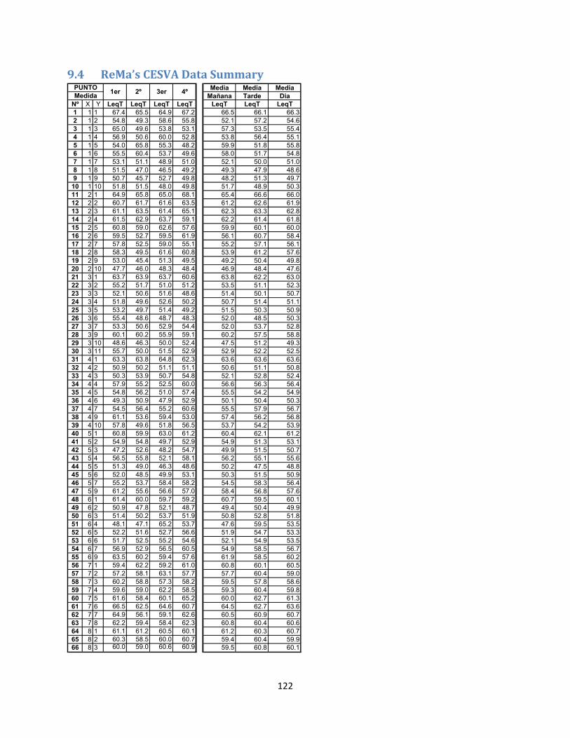
122

9.4 ReMa’s CESVA Data Summary Media Media Media

Mañana Tarde DiaNº X Y LeqT LeqT LeqT LeqT LeqT LeqT LeqT1 1 1 67.4 65.5 64.9 67.2 66.5 66.1 66.32 1 2 54.8 49.3 58.6 55.8 52.1 57.2 54.63 1 3 65.0 49.6 53.8 53.1 57.3 53.5 55.44 1 4 56.9 50.6 60.0 52.8 53.8 56.4 55.15 1 5 54.0 65.8 55.3 48.2 59.9 51.8 55.86 1 6 55.5 60.4 53.7 49.6 58.0 51.7 54.87 1 7 53.1 51.1 48.9 51.0 52.1 50.0 51.08 1 8 51.5 47.0 46.5 49.2 49.3 47.9 48.69 1 9 50.7 45.7 52.7 49.8 48.2 51.3 49.710 1 10 51.8 51.5 48.0 49.8 51.7 48.9 50.311 2 1 64.9 65.8 65.0 68.1 65.4 66.6 66.012 2 2 60.7 61.7 61.6 63.5 61.2 62.6 61.913 2 3 61.1 63.5 61.4 65.1 62.3 63.3 62.814 2 4 61.5 62.9 63.7 59.1 62.2 61.4 61.815 2 5 60.8 59.0 62.6 57.6 59.9 60.1 60.016 2 6 59.5 52.7 59.5 61.9 56.1 60.7 58.417 2 7 57.8 52.5 59.0 55.1 55.2 57.1 56.118 2 8 58.3 49.5 61.6 60.8 53.9 61.2 57.619 2 9 53.0 45.4 51.3 49.5 49.2 50.4 49.820 2 10 47.7 46.0 48.3 48.4 46.9 48.4 47.621 3 1 63.7 63.9 63.7 60.6 63.8 62.2 63.022 3 2 55.2 51.7 51.0 51.2 53.5 51.1 52.323 3 3 52.1 50.6 51.6 48.6 51.4 50.1 50.724 3 4 51.8 49.6 52.6 50.2 50.7 51.4 51.125 3 5 53.2 49.7 51.4 49.2 51.5 50.3 50.926 3 6 55.4 48.6 48.7 48.3 52.0 48.5 50.327 3 7 53.3 50.6 52.9 54.4 52.0 53.7 52.828 3 9 60.1 60.2 55.9 59.1 60.2 57.5 58.829 3 10 48.6 46.3 50.0 52.4 47.5 51.2 49.330 3 11 55.7 50.0 51.5 52.9 52.9 52.2 52.531 4 1 63.3 63.8 64.8 62.3 63.6 63.6 63.632 4 2 50.9 50.2 51.1 51.1 50.6 51.1 50.833 4 3 50.3 53.9 50.7 54.8 52.1 52.8 52.434 4 4 57.9 55.2 52.5 60.0 56.6 56.3 56.435 4 5 54.8 56.2 51.0 57.4 55.5 54.2 54.936 4 6 49.3 50.9 47.9 52.9 50.1 50.4 50.337 4 7 54.5 56.4 55.2 60.6 55.5 57.9 56.738 4 9 61.1 53.6 59.4 53.0 57.4 56.2 56.839 4 10 57.8 49.6 51.8 56.5 53.7 54.2 53.940 5 1 60.8 59.9 63.0 61.2 60.4 62.1 61.241 5 2 54.9 54.8 49.7 52.9 54.9 51.3 53.142 5 3 47.2 52.6 48.2 54.7 49.9 51.5 50.743 5 4 56.5 55.8 52.1 58.1 56.2 55.1 55.644 5 5 51.3 49.0 46.3 48.6 50.2 47.5 48.845 5 6 52.0 48.5 49.9 53.1 50.3 51.5 50.946 5 7 55.2 53.7 58.4 58.2 54.5 58.3 56.447 5 9 61.2 55.6 56.6 57.0 58.4 56.8 57.648 6 1 61.4 60.0 59.7 59.2 60.7 59.5 60.149 6 2 50.9 47.8 52.1 48.7 49.4 50.4 49.950 6 3 51.4 50.2 53.7 51.9 50.8 52.8 51.851 6 4 48.1 47.1 65.2 53.7 47.6 59.5 53.552 6 5 52.2 51.6 52.7 56.6 51.9 54.7 53.353 6 6 51.7 52.5 55.2 54.6 52.1 54.9 53.554 6 7 56.9 52.9 56.5 60.5 54.9 58.5 56.755 6 9 63.5 60.2 59.4 57.6 61.9 58.5 60.256 7 1 59.4 62.2 59.2 61.0 60.8 60.1 60.557 7 2 57.2 58.1 63.1 57.7 57.7 60.4 59.058 7 3 60.2 58.8 57.3 58.2 59.5 57.8 58.659 7 4 59.6 59.0 62.2 58.5 59.3 60.4 59.860 7 5 61.6 58.4 60.1 65.2 60.0 62.7 61.361 7 6 66.5 62.5 64.6 60.7 64.5 62.7 63.662 7 7 64.9 56.1 59.1 62.6 60.5 60.9 60.763 7 8 62.2 59.4 58.4 62.3 60.8 60.4 60.664 8 1 61.1 61.2 60.5 60.1 61.2 60.3 60.765 8 2 60.3 58.5 60.0 60.7 59.4 60.4 59.966 8 3 60.0 59.0 60.6 60.9 59.5 60.8 60.1

4ºMedidaPUNTO 1er 2º 3er

123

9.4.1 ReMa’s CESVA First Interval Nº X Y Dia Inicio L10 L90 MaxLF LeqT MaxLeq1m1 1 1 11/28/2012 8:03 70.6 60.8 79.4 67.4 69.92 1 2 11/28/2012 9:20 56.6 51.8 71.1 54.8 57.53 1 3 11/28/2012 9:12 67.2 57.0 70.5 65.0 66.64 1 4 11/28/2012 9:04 57.3 51.2 74.2 56.9 60.55 1 5 11/28/2012 8:56 54.9 50.4 70.8 54.0 55.96 1 6 11/28/2012 8:49 56.8 51.6 71.0 55.5 57.47 1 7 11/28/2012 8:41 55.2 49.7 65.4 53.1 54.98 1 8 11/28/2012 8:34 53.2 49.3 68.0 51.5 52.39 1 9 11/28/2012 8:26 52.0 49.1 60.4 50.7 51.510 1 10 11/28/2012 8:19 53.6 49.3 59.6 51.8 52.811 2 1 11/28/2012 9:30 68.5 57.2 83.0 64.9 66.812 2 2 11/28/2012 9:38 64.4 52.6 72.9 60.7 61.813 2 3 11/28/2012 9:45 62.8 49.7 77.1 61.1 62.714 2 4 11/28/2012 9:54 64.7 49.2 76.0 61.5 64.215 2 5 11/28/2012 10:02 62.5 48.6 77.7 60.8 62.416 2 6 11/28/2012 10:10 59.9 47.5 77.2 59.5 63.517 2 7 11/28/2012 10:17 61.1 49.8 71.7 57.8 61.018 2 8 11/28/2012 10:25 55.3 49.1 78.0 58.3 62.519 2 9 11/28/2012 10:33 55.4 48.9 62.1 53.0 55.020 2 10 11/28/2012 10:40 49.2 45.8 52.4 47.7 48.221 3 1 11/27/2012 8:13 66.9 55.6 82.5 63.7 66.922 3 2 11/27/2012 8:22 55.8 50.8 73.0 55.2 59.023 3 3 11/27/2012 8:30 52.8 48.4 76.7 52.1 54.524 3 4 11/27/2012 8:41 53.3 49.1 63.7 51.8 53.525 3 5 11/27/2012 8:51 55.1 50.7 62.6 53.2 54.426 3 6 11/27/2012 9:00 59.0 48.4 66.3 55.4 58.427 3 7 11/27/2012 9:28 56.2 50.1 62.8 53.3 54.728 3 9 11/28/2012 11:05 56.7 46.8 82.1 60.1 63.429 3 10 11/28/2012 10:57 50.5 46.2 55.6 48.6 49.530 3 11 11/28/2012 10:49 54.6 47.7 81.7 55.7 61.231 4 1 11/27/2012 10:36 67.1 54.3 73.3 63.3 65.532 4 2 11/27/2012 10:26 53.3 46.4 62.8 50.9 52.533 4 3 11/27/2012 10:11 50.9 49.5 57.9 50.3 51.134 4 4 11/27/2012 10:04 59.5 50.2 76.9 57.9 62.235 4 5 11/27/2012 9:54 57.3 51.5 62.9 54.8 56.136 4 6 11/27/2012 9:45 51.4 46.3 61.3 49.3 50.037 4 7 11/27/2012 9:37 57.0 48.9 67.8 54.5 55.638 4 9 11/30/2012 8:13 61.3 51.1 79.4 61.1 63.639 4 10 11/30/2012 8:04 61.0 50.7 67.4 57.8 59.640 5 1 11/27/2012 10:45 63.2 55.2 70.7 60.8 61.741 5 2 11/27/2012 10:53 58.4 48.0 67.8 54.9 57.042 5 3 11/27/2012 11:00 48.4 45.6 64.1 47.2 47.543 5 4 11/27/2012 11:10 59.6 47.4 71.8 56.5 59.644 5 5 12/3/2012 9:45 53.5 48.4 63.9 51.3 51.945 5 6 12/3/2012 9:59 53.5 50.2 59.7 52.0 52.646 5 7 12/3/2012 10:30 58.3 48.9 67.6 55.2 57.347 5 9 11/30/2012 8:23 63.1 53.3 76.5 61.2 62.948 6 1 11/30/2012 10:24 64.9 50.4 77.9 61.4 62.649 6 2 11/30/2012 10:33 52.9 47.0 63.9 50.9 52.050 6 3 11/30/2012 10:43 53.9 47.6 63.2 51.4 52.451 6 4 11/30/2012 10:54 50.2 45.3 61.4 48.1 50.152 6 5 11/30/2012 11:08 52.8 42.2 73.2 52.2 57.553 6 6 12/3/2012 10:07 53.2 48.4 63.2 51.7 52.754 6 7 12/3/2012 10:24 60.0 51.4 70.9 56.9 58.855 6 9 11/30/2012 8:32 65.0 54.7 78.9 63.5 65.356 7 1 11/30/2012 10:15 63.4 52.2 71.5 59.4 61.957 7 2 11/30/2012 9:55 60.2 48.4 70.7 57.2 58.658 7 3 11/30/2012 9:28 64.3 49.6 72.8 60.2 61.059 7 4 11/30/2012 9:19 60.8 56.7 72.0 59.6 60.460 7 5 11/30/2012 9:10 65.6 51.6 78.4 61.6 63.761 7 6 11/30/2012 9:00 70.8 54.2 80.3 66.5 68.662 7 7 11/30/2012 8:51 66.8 61.2 81.5 64.9 65.463 7 8 11/30/2012 8:41 63.4 55.6 78.3 62.2 65.364 8 1 11/30/2012 10:05 63.3 57.4 70.1 61.1 61.965 8 2 11/30/2012 9:46 63.0 54.1 66.2 60.3 61.166 8 3 11/30/2012 9:38 63.6 54.2 67.5 60.0 61.2

124

9.4.2 ReMa’s CESVA Second Interval Nº X Y Dia Inicio L10 L90 MaxLF LeqT MaxLeq1m1 1 1 11/26/2012 11:21 69.3 54.4 76.3 65.5 66.42 1 2 11/26/2012 11:29 50.7 47.6 56.5 49.3 50.13 1 3 11/26/2012 11:38 50.8 46.9 62.4 49.6 52.04 1 4 11/26/2012 11:48 47.4 45.0 69.1 50.6 56.35 1 5 11/26/2012 11:58 69.5 50.8 76.1 65.8 68.36 1 6 11/26/2012 12:09 63.5 47.5 68.7 60.4 61.47 1 7 11/26/2012 12:20 50.7 45.0 68.2 51.1 55.88 1 8 11/26/2012 12:30 48.2 45.7 53.7 47.0 47.89 1 9 11/26/2012 12:38 46.3 45.0 54.1 45.7 45.910 1 10 11/26/2012 12:48 51.2 44.5 66.9 51.5 57.411 2 1 11/26/2012 14:19 68.5 56.5 81.4 65.8 69.312 2 2 11/26/2012 14:10 65.3 50.0 75.8 61.7 62.813 2 3 11/26/2012 14:02 68.0 46.8 79.0 63.5 65.714 2 4 11/26/2012 13:54 66.4 47.4 78.7 62.9 65.815 2 5 11/26/2012 13:45 61.0 45.9 75.4 59.0 61.516 2 6 11/26/2012 13:36 57.3 44.4 67.3 52.7 55.317 2 7 11/26/2012 13:27 55.1 46.7 72.5 52.5 54.518 2 8 11/26/2012 13:17 49.4 42.7 69.5 49.5 55.019 2 9 11/26/2012 13:10 46.7 43.9 51.4 45.4 46.020 2 10 11/26/2012 12:57 47.4 44.3 52.5 46.0 47.021 3 1 11/26/2012 14:25 67.8 52.6 79.8 63.9 65.922 3 2 11/27/2012 13:55 54.5 45.7 65.2 51.7 54.823 3 3 11/27/2012 13:47 53.2 46.4 69.9 50.6 51.724 3 4 11/27/2012 13:38 51.5 42.6 65.5 49.6 52.125 3 5 11/27/2012 13:30 52.2 44.8 59.1 49.7 51.426 3 6 11/27/2012 13:21 51.5 41.5 63.2 48.6 50.727 3 7 11/27/2012 13:13 53.5 42.6 65.5 50.6 53.428 3 9 11/27/2012 13:01 48.2 43.6 83.8 60.2 67.129 3 10 11/27/2012 12:54 47.8 44.5 52.7 46.3 47.930 3 11 11/27/2012 12:40 52.9 44.1 58.7 50.0 51.831 4 1 11/27/2012 14:06 67.3 53.9 74.1 63.8 65.032 4 2 11/27/2012 14:15 52.6 46.3 63.5 50.2 51.933 4 3 11/27/2012 14:26 55.3 48.7 71.5 53.9 57.834 4 4 11/28/2012 11:45 58.3 50.0 70.0 55.2 56.335 4 5 11/28/2012 11:37 58.6 51.8 68.6 56.2 57.536 4 6 11/28/2012 11:29 52.0 47.1 74.3 50.9 53.637 4 7 11/28/2012 11:20 59.1 50.0 73.5 56.4 59.438 4 9 11/27/2012 12:24 52.5 47.1 71.0 53.6 56.939 4 10 11/27/2012 12:31 52.3 44.4 54.9 49.6 51.540 5 1 11/30/2012 14:01 63.1 53.3 71.3 59.9 62.441 5 2 11/30/2012 13:53 56.7 49.0 69.3 54.8 57.842 5 3 11/30/2012 13:44 56.2 45.3 65.7 52.6 54.043 5 4 11/30/2012 13:35 59.4 45.5 70.1 55.8 59.044 5 5 11/27/2012 11:18 50.6 46.7 56.3 49.0 49.745 5 6 11/27/2012 11:26 50.8 44.9 58.7 48.5 49.646 5 7 11/27/2012 11:34 57.6 47.4 65.6 53.7 55.047 5 9 11/27/2012 12:15 54.9 47.3 77.1 55.6 61.148 6 1 11/30/2012 12:04 64.1 50.3 72.6 60.0 62.449 6 2 11/30/2012 11:54 49.3 45.9 56.4 47.8 48.550 6 3 11/30/2012 11:45 53.0 45.8 60.7 50.2 52.151 6 4 11/30/2012 11:35 49.0 42.1 63.4 47.1 50.852 6 5 11/30/2012 11:26 52.7 42.8 67.8 51.6 54.053 6 6 11/30/2012 11:16 57.2 42.8 67.5 52.5 56.654 6 7 11/27/2012 11:43 55.9 45.0 72.1 52.9 55.055 6 9 11/27/2012 12:08 62.1 47.8 76.2 60.2 64.456 7 1 11/30/2012 12:12 65.6 53.7 74.7 62.2 64.157 7 2 11/30/2012 12:30 61.3 47.8 72.0 58.1 59.058 7 3 11/30/2012 12:56 61.4 48.4 75.0 58.8 62.559 7 4 11/30/2012 13:05 62.8 52.9 73.4 59.0 61.160 7 5 11/30/2012 13:14 60.5 47.3 75.3 58.4 60.761 7 6 11/30/2012 13:23 67.0 48.8 77.4 62.5 64.362 7 7 11/27/2012 11:54 59.4 50.6 66.8 56.1 58.463 7 8 11/27/2012 12:01 58.5 47.1 77.9 59.4 62.964 8 1 11/30/2012 12:21 64.3 56.9 69.7 61.2 62.265 8 2 11/30/2012 12:39 61.8 51.3 66.7 58.5 59.466 8 3 11/30/2012 12:48 61.8 54.1 67.0 59.0 60.1

125

9.4.3 ReMa’s CESVA Third Interval Nº X Y Dia Inicio L10 L90 MaxLF LeqT MaxLeq1m1 1 1 11/27/2012 16:17 68.2 56.8 79.4 64.9 67.42 1 2 11/27/2012 16:28 55.8 49.2 78.1 58.6 64.53 1 3 11/27/2012 16:36 53.4 47.6 73.0 53.8 59.24 1 4 11/27/2012 16:45 63.9 47.1 74.5 60.0 64.95 1 5 11/27/2012 16:53 55.8 48.1 76.1 55.3 61.06 1 6 11/27/2012 17:01 49.3 44.6 75.5 53.7 58.77 1 7 11/27/2012 17:10 51.5 44.2 63.2 48.9 51.28 1 8 11/27/2012 17:18 48.2 43.0 63.3 46.5 49.49 1 9 11/27/2012 17:25 51.9 46.0 67.1 52.7 58.310 1 10 11/27/2012 17:32 49.5 46.1 55.0 48.0 48.611 2 1 12/3/2012 16:00 69.2 55.9 75.1 65.0 66.412 2 2 12/3/2012 15:51 65.1 48.9 77.6 61.6 64.213 2 3 12/3/2012 15:42 63.5 45.3 78.4 61.4 64.714 2 4 11/27/2012 18:37 67.8 49.5 78.9 63.7 66.615 2 5 11/27/2012 18:30 66.4 48.8 79.3 62.6 64.216 2 6 11/27/2012 18:15 62.4 48.3 77.7 59.5 62.017 2 7 11/27/2012 18:07 62.0 51.4 73.3 59.0 63.418 2 8 11/27/2012 17:59 61.8 48.1 80.5 61.6 64.819 2 9 11/27/2012 17:49 53.9 47.8 57.5 51.3 53.820 2 10 11/27/2012 17:40 50.1 46.3 59.0 48.3 48.721 3 1 12/3/2012 16:09 67.3 51.6 77.8 63.7 64.922 3 2 11/26/2012 15:39 53.8 46.8 60.1 51.0 52.423 3 3 11/26/2012 15:47 52.5 47.1 69.1 51.6 55.524 3 4 11/26/2012 15:55 56.7 45.9 61.9 52.6 54.125 3 5 11/26/2012 16:05 53.1 45.6 66.0 51.4 53.426 3 6 11/26/2012 16:14 50.2 45.8 65.8 48.7 51.527 3 7 11/26/2012 16:21 56.2 47.6 69.1 52.9 55.028 3 9 11/26/2012 16:34 56.6 46.3 75.2 55.9 62.129 3 10 11/26/2012 16:43 52.1 47.0 61.8 50.0 50.530 3 11 11/26/2012 16:52 54.3 47.7 64.2 51.5 54.331 4 1 11/30/2012 16:34 67.8 55.4 80.8 64.8 67.832 4 2 11/30/2012 16:26 53.6 47.3 64.6 51.1 53.733 4 3 11/30/2012 16:17 51.8 48.1 67.3 50.7 52.934 4 4 11/30/2012 16:09 51.6 46.9 71.3 52.5 57.435 4 5 11/30/2012 16:00 53.2 48.0 63.0 51.0 51.736 4 6 11/30/2012 15:51 50.4 43.5 61.3 47.9 50.237 4 7 11/30/2012 15:43 58.8 47.2 71.4 55.2 57.838 4 9 11/26/2012 17:10 60.8 46.0 75.8 59.4 62.639 4 10 11/26/2012 17:00 53.5 49.6 58.5 51.8 52.540 5 1 11/30/2012 16:44 65.3 54.8 77.3 63.0 64.441 5 2 11/30/2012 16:53 49.8 43.5 67.0 49.7 53.242 5 3 11/30/2012 17:01 51.1 42.5 60.3 48.2 50.843 5 4 11/30/2012 17:10 52.4 44.1 70.0 52.1 56.544 5 5 11/30/2012 17:19 47.4 44.7 56.7 46.3 47.945 5 6 11/30/2012 17:27 51.5 47.2 60.0 49.9 52.646 5 7 11/30/2012 17:36 60.9 51.7 72.6 58.4 60.847 5 9 11/26/2012 17:20 56.7 46.8 74.7 56.6 59.948 6 1 11/30/2012 18:42 63.3 52.6 73.1 59.7 61.449 6 2 11/30/2012 18:34 53.3 50.3 65.8 52.1 52.950 6 3 11/30/2012 18:25 55.4 51.5 67.8 53.7 54.651 6 4 11/30/2012 18:11 66.9 63.0 73.2 65.2 67.152 6 5 11/30/2012 18:00 54.4 50.2 63.0 52.7 53.653 6 6 11/30/2012 17:53 56.3 51.5 72.1 55.2 56.554 6 7 11/30/2012 17:44 60.0 50.2 69.8 56.5 58.255 6 9 11/26/2012 17:28 59.0 47.2 78.3 59.4 64.156 7 1 12/3/2012 16:20 63.0 51.4 73.3 59.2 61.457 7 2 12/3/2012 16:45 61.7 49.4 85.4 63.1 68.058 7 3 11/26/2012 17:30 59.0 48.1 75.4 57.3 60.859 7 4 11/26/2012 18:20 64.1 60.2 72.9 62.2 63.660 7 5 11/26/2012 18:11 62.9 46.0 75.5 60.1 63.561 7 6 11/26/2012 18:05 68.8 48.8 79.6 64.6 67.062 7 7 11/26/2012 17:47 62.6 52.3 68.8 59.1 61.463 7 8 11/26/2012 17:36 62.2 47.6 75.5 58.4 63.264 8 1 12/3/2012 16:29 63.3 55.8 69.9 60.5 62.665 8 2 12/3/2012 16:37 63.0 54.1 67.3 60.0 61.166 8 3 11/26/2012 18:38 62.9 56.1 67.6 60.6 61.3

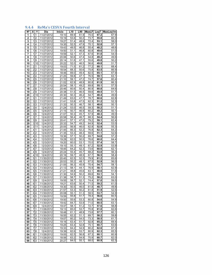
126

9.4.4 ReMa’s CESVA Fourth Interval Nº X Y Dia Inicio L10 L90 MaxLF LeqT MaxLeq1m1 1 1 11/27/2012 19:10 69.9 61.9 75.0 67.2 67.92 1 2 11/27/2012 19:19 53.6 50.2 73.7 55.8 60.33 1 3 11/27/2012 19:27 51.4 48.9 72.4 53.1 58.04 1 4 11/27/2012 19:35 52.5 47.9 70.1 52.8 57.15 1 5 11/27/2012 19:43 49.5 46.8 55.4 48.2 48.66 1 6 11/27/2012 19:50 51.1 46.8 60.8 49.6 51.07 1 7 11/27/2012 19:59 52.1 47.3 67.6 51.0 54.08 1 8 11/27/2012 20:06 50.6 47.4 54.8 49.2 49.69 1 9 11/27/2012 20:14 51.6 47.1 55.6 49.8 50.210 1 10 11/27/2012 20:22 52.0 46.5 56.6 49.8 51.711 2 1 11/27/2012 19:03 71.5 61.2 77.2 68.1 68.412 2 2 11/27/2012 18:54 68.3 50.6 75.8 63.5 66.913 2 3 11/27/2012 18:46 69.0 49.4 82.5 65.1 67.914 2 4 11/27/2012 21:25 59.8 47.1 76.5 59.1 63.115 2 5 11/27/2012 21:10 59.1 47.2 74.7 57.6 60.416 2 6 11/27/2012 21:02 62.9 48.9 80.8 61.9 66.317 2 7 11/27/2012 20:54 58.1 49.2 69.8 55.1 57.518 2 8 11/27/2012 20:46 60.6 50.4 80.9 60.8 64.619 2 9 11/27/2012 20:38 51.5 46.5 59.6 49.5 51.720 2 10 11/27/2012 20:30 50.3 46.2 54.7 48.4 49.621 3 1 11/27/2012 21:49 63.0 47.7 78.7 60.6 62.822 3 2 11/27/2012 21:41 53.8 47.5 62.3 51.2 52.323 3 3 11/27/2012 21:33 50.3 46.7 58.1 48.6 50.124 3 4 12/4/2012 21:24 53.0 46.5 59.3 50.2 51.125 3 5 12/4/2012 21:15 50.7 46.9 60.2 49.2 50.126 3 6 12/4/2012 21:07 50.3 45.7 57.9 48.3 49.027 3 7 12/4/2012 20:58 56.4 46.7 68.3 54.4 56.628 3 9 12/4/2012 20:41 57.1 47.0 79.2 59.1 62.429 3 10 12/4/2012 20:33 54.7 49.2 64.9 52.4 53.030 3 11 12/4/2012 20:05 56.9 46.0 62.8 52.9 55.331 4 1 12/4/2012 21:45 66.3 52.2 76.8 62.3 64.232 4 2 12/4/2012 21:35 53.3 48.3 59.6 51.1 52.633 4 3 12/3/2012 19:36 57.1 50.2 69.7 54.8 57.234 4 4 12/3/2012 19:28 62.0 50.5 76.6 60.0 64.435 4 5 12/3/2012 19:20 60.0 53.1 70.0 57.4 58.736 4 6 12/3/2012 19:10 55.1 49.1 67.2 52.9 53.937 4 7 12/3/2012 18:45 64.2 52.3 73.6 60.6 62.138 4 9 12/4/2012 20:24 55.4 45.7 68.2 53.0 56.339 4 10 12/4/2012 20:16 59.7 48.5 67.7 56.5 58.440 5 1 11/30/2012 20:45 62.5 52.5 79.9 61.2 65.641 5 2 11/30/2012 20:53 55.2 48.1 67.5 52.9 56.042 5 3 11/30/2012 21:05 56.3 45.9 70.4 54.7 58.143 5 4 11/30/2012 21:13 58.1 44.1 76.9 58.1 62.944 5 5 11/30/2012 21:21 48.8 45.6 63.1 48.6 51.645 5 6 11/30/2012 21:30 54.9 50.2 69.6 53.1 54.146 5 7 11/30/2012 21:38 58.7 51.3 75.2 58.2 63.047 5 9 12/4/2012 19:55 58.7 52.1 74.4 57.0 59.548 6 1 11/26/2012 19:21 63.6 50.4 71.5 59.2 61.049 6 2 11/26/2012 19:30 50.5 46.0 61.8 48.7 49.850 6 3 11/30/2012 21:57 53.3 50.2 61.8 51.9 52.651 6 4 11/30/2012 20:08 55.1 51.3 59.5 53.7 54.952 6 5 11/30/2012 19:59 55.8 51.7 78.4 56.6 60.553 6 6 11/30/2012 19:50 55.6 53.3 60.8 54.6 54.954 6 7 11/30/2012 19:42 64.7 53.9 71.0 60.5 63.155 6 9 12/4/2012 19:47 58.1 51.2 72.7 57.6 58.856 7 1 11/26/2012 19:13 65.0 53.7 70.8 61.0 62.657 7 2 11/26/2012 18:48 61.1 48.9 73.6 57.7 60.158 7 3 11/30/2012 18:55 62.2 51.1 69.7 58.2 59.859 7 4 11/30/2012 19:07 60.2 54.5 73.3 58.5 61.760 7 5 11/30/2012 19:16 63.4 51.7 92.8 65.2 69.461 7 6 11/30/2012 19:25 63.4 52.8 75.1 60.7 63.662 7 7 11/30/2012 19:33 64.2 54.9 80.2 62.6 67.363 7 8 12/4/2012 19:39 62.6 53.7 80.9 62.3 65.564 8 1 11/26/2012 19:05 62.5 56.8 67.3 60.1 60.965 8 2 11/26/2012 18:56 63.2 54.9 70.9 60.7 62.066 8 3 11/30/2012 20:27 64.0 55.1 68.0 60.9 62.3

127

9.5 Noise Source Data

9.5.1 Noise Point Sources ID DESCRIPTION LOUDNESS HEIGHT WIDTH MEAN MAX

1 VENT NOTICEABLE 3 STORY 9M 55.9 60.92 PELIGRO LOUD 1 STORY 9M 62.1 633 CONSTRUCTION MACHINERY (BORER AND BACKHOE) VERY LOUD 1 STORY 27M 75 754 PELIGRO LOUD 1 STORY 3M 60.7 61.25 VENT VERY LOUD 1 STORY 3M 66.2 71.56 PELIGRO LOUD EYE LEVEL 3M 60.5 61.27 AV VENT NOTICEABLE EYE LEVEL 3M 60.4 65.58 HIGH PITCHED VERY LOUD 3 STORY 9M 61 619 VENT NOTICEABLE EYE LEVEL 4M 63.1 65.1

10 4 FANS, 1 BLOWING, MUSIC AND DISHES VERY LOUD EYE LEVEL 3M 62.1 7011 PELIGRO LOUD 1 STORY 3M 68.1 68.512 FAN, DISHES, TALKING SLIGHT 1 STORY 1M 60 64.413 PELIGRO LOUD 1 STORY 3M 63.6 66.414 VENT NOTICEABLE 5 STORY 2M 49 52.315 VENT LOUD 1 STORY 2M 59.9 60.316 FOUNTAIN LOUD GROUND 9M 62.9 65.617 FOUNTAIN VERY LOUD EYE LEVEL 2M 64.8 70.718 2 FAN WINDOW UNITS LOUD 3 STORY 1M 57.4 58.919 MULTIPLE VENTS VERY LOUD 2 STORY 9M 77.9 79.220 VENT LOUD BASEMENT 3M 66.4 66.821 PELIGRO LOUD 1 STORY 3M 51.4 55.122 GARDENING SAW VERY LOUD EYE LEVEL POINT 75 78.223 BICICAS STATION NOTICEABLE 1 STORY POINT 65.5 66.424 PELIGRO SLIGHT 1 STORY 1M 58.9 62.725 BICICAS STATION SLIGHT EYE LEVEL POINT 58.6 59.626 PELIGRO SLIGHT 1 STORY 2M 54.8 56.827 MAINTENANCE EQUIPMENT LOUD 1 STORY 2M 64.7 66.428 2 FANS VERY LOUD EYE LEVEL 1M 78 79.729 PELIGRO LOUD 1 STORY 1M 55.5 56.630 BICICAS STATION NOTICEABLE 1 STORY POINT 61.3 63.731 CONSTRUCTION MACHINERY (BORER) NOTICEABLE 1 STORY 9M 75 7532 LARGE FANS VERY LOUD 1 STORY 9M 75 75

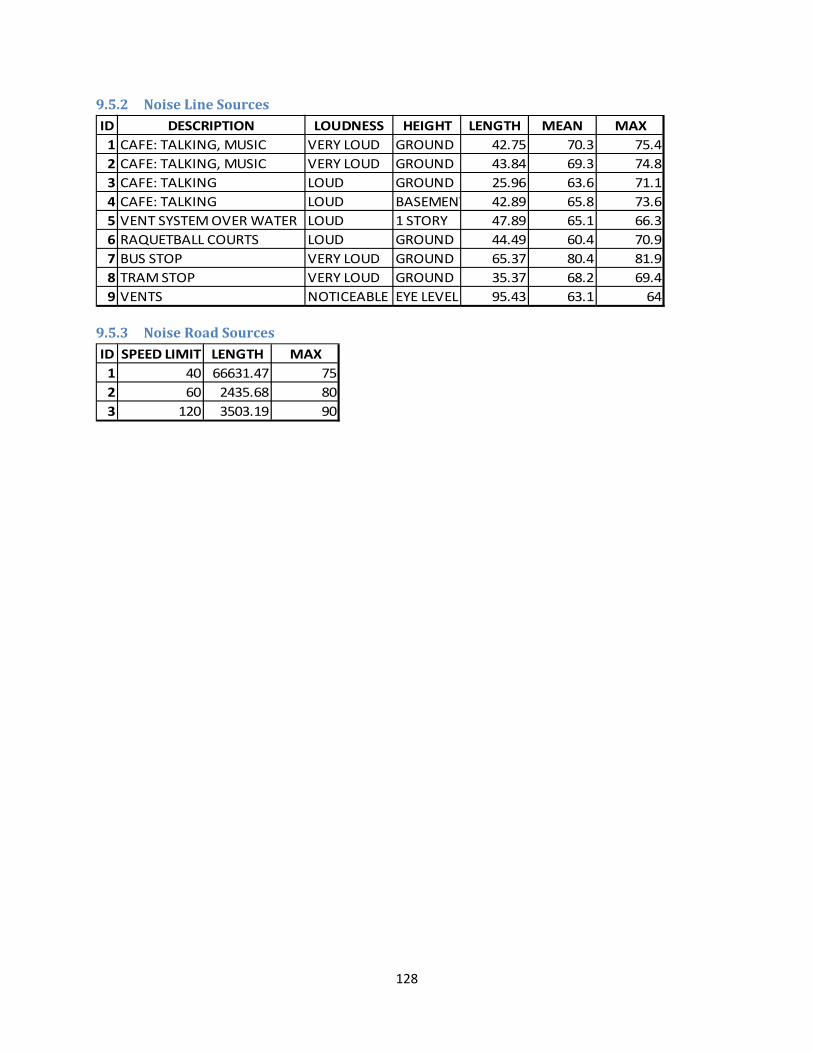
128

9.5.2 Noise Line Sources ID DESCRIPTION LOUDNESS HEIGHT LENGTH MEAN MAX

1 CAFE: TALKING, MUSIC VERY LOUD GROUND 42.75 70.3 75.42 CAFE: TALKING, MUSIC VERY LOUD GROUND 43.84 69.3 74.83 CAFE: TALKING LOUD GROUND 25.96 63.6 71.14 CAFE: TALKING LOUD BASEMENT 42.89 65.8 73.65 VENT SYSTEM OVER WATER LOUD 1 STORY 47.89 65.1 66.36 RAQUETBALL COURTS LOUD GROUND 44.49 60.4 70.97 BUS STOP VERY LOUD GROUND 65.37 80.4 81.98 TRAM STOP VERY LOUD GROUND 35.37 68.2 69.49 VENTS NOTICEABLE EYE LEVEL 95.43 63.1 64

9.5.3 Noise Road Sources ID SPEED LIMIT LENGTH MAX

1 40 66631.47 752 60 2435.68 803 120 3503.19 90

129

10. Plagiarism Declaration

I hereby confirm that the words and work in this thesis, Strategic noise mapping with GIS for the Universitat Jaume I Smart Campus: Best methodology practices, are original and my own. All outside information and ideas are cited properly in the References section.

I also confirm that this work has not been previously submitted to any other university or institution.

Sincerely,

Sarah Eason

Date:

130

Strategic noise mapping with GIS for the Universitat Jaume I Smart Campus: 2013 Best methodology practices Sarah Eason

131

Sarah Eason

Strategic noise mapping with GIS for the Universitat Jaume ...

Documents

Transcript of Strategic noise mapping with GIS for the Universitat Jaume ...