CCITT | 600 Foster Street | Evanston, IL 60208 Tel: 847-491-7287 | Fax: 847-491-3090

http://www.ccitt.northwestern.edu/

Strategic Gang Scheduling for Railroad Maintenance

August 14, 2012

Conrado Borraz-Sánchez, Diego Klabjan

Department of Industrial Engineering and Management Sciences, Northwestern University

DISCLAIMER: The contents of this report reflect the views of the authors, who are responsible for the facts and the accuracy of the information presented herein. This document is disseminated under the sponsorship of the Department of Transportation University

Transportation Centers Program, in the interest of information exchange. The U.S. Government assumes no liability for the contents or use thereof.

This work was funded by the Center for the Commercialization of Innovative Transportation Technology at Northwestern University, a University Transportation Center Program of the Research and Innovative Technology Administration of USDOT through support from the Safe, Accountable, Flexible, Efficient

Transportation Equity Act (SAFETEA‐LU).

Strategic Gang Scheduling for Railroad Maintenance

Conrado Borraz-Sanchez, Diego KlabjanDepartment of Industrial Engineering and Management Sciences, Northwestern University, Evanston, IL 60208

{c-borraz-sanchez, d-klabjan}@northwestern.edu

Abstract: We address the railway track maintenance scheduling problem. The problem stems from thesignificant percentage of the annual budget invested by the railway industry for maintaining its railwaytracks. The process requires consideration of human resource allocations (gangs), as well as effective logisticsfor equipment movement and routing around the rail network under time window constraints. We proposean efficient solution approach to minimize total costs incurred by the maintenance projects or jobs withina given planning horizon. This is accomplished by designing a job-time network model to capture feasibleschedules under the constraints of job precedence and developing a mathematical programming heuristic tosolve the underlying model. The key ingredient is an iterative process that extracts and then re-inserts jobsbased on an integer programming model. Computational experiments show the capability of the proposedheuristic to schedule more than 1,000 jobs and more than 30 gangs.

Keywords : Railway Maintenance, Integer Programming, Heuristics

1. Introduction

Since the inception of the railway industry during the Industrial Revolution, the industry hasevolved into a vital means of transportation worldwide. The US railway industry nowadays ownsan intensive infrastructure that requires constant maintenance and improvements. In the US, arailway owns the tracks and has to maintain them. Such a business model is the focus of this paper.In Europe, a track is shared by many railways, which require different maintenance agreements.

By taking into account its tens of thousands of miles of tracks, which are subject to wearand failures due to their extensive use, the railway industry must judiciously plan its day-to-dayplanning problems and the preceding tactical challenges. This fact is supported by the equipmentand labor intensive processes typically conducted throughout a year for the maintenance of tracks,including both preventive and real-time maintenance.

According to TATA Consultancy Services (2002), the American Public Transportation Associa-tion (APTA) estimates that track maintenance expenditures comprise roughly 9% of total operatingcosts, from which nearly 80% corresponds to labor cost. In monetary terms these numbers maycorrespond to millions of dollars on annual maintenance projects (Judge, 2010).

Maintenance workers work in groups, called gangs, performing heavy labor duties such asinstalling track ties, driving track spikes, shoveling ballast and other similar maintenance trackrelated activities. A gang consists of several members (between 10–100) with different responsi-bilities such as machine operators, termite welders, assistant extra gang foreman, or extra gangforeman. A gang beat or a beat section is a section of a track assigned to a gang to work on. Duringa year a gang moves from one beat section (a job) to another upon completion of the work at thesection.

The railway maintenance scheduling problem (RMSP) is to find a sequence of jobs to be assignedto each gang over a time horizon (typically one year). Together with such an assignment, for eachjob a start and finish date must be determined. The goal is to minimize the overall cost whileobeying various business requirements (e.g., certain jobs must be performed before other, a gangcan only perform a job based on qualifications, etc.).

1

2

The RMSP is typically solved a few months before the start of the planning horizon, i.e., duringthe summer for the next calendar year.

A Class–1 US railway typically undertakes an intensive effort to determine and sustain annualrail maintenance schedules. This scheduling process is often labor intensive and leads to a costly andsub-optimal schedule. In this paper we propose a solution approach to efficiently solve the RMSP.We develop an algorithm that focuses on three specific issues: 1) minimize the total cost incurredby all track maintenance projects conducted throughout a given planning horizon, including costof transition between jobs and cost of equipment movement between two locations, as well as costof travel between a job location and the home-base of a gang, 2) provide practical feasible solutionsthat obey all business requirements, for example, it is required for gangs to work at a southernarea during a winter season, 3) to be capable of computationally handling large-scale instances,such as those posed by Class–1 US railways.

More precisely, our solution methodology is based on a mathematical programming heuristic thatis based on a job-time network model designed for each gang type. The network model basicallycaptures feasible schedules, i.e., each schedule corresponds to a path (reverse not being true).As a result of solving the underlying model, our heuristic provides a maintenance schedule thatoutperforms current industry practice.

The RMSP differs from other maintenance problems by the heavy machinery being used andthe large number of crew members that are involved in the track maintenance projects. One of themost distinct characteristics from its highway counterpart is the large spatial area to be coveredby the whole maintenance schedule, i.e., it typically spans the entire railway network. In addition,ongoing track maintenance projects may imply curfew in certain sections and train schedules mustbe altered. Hence, a large number of specific business rules (side constraints) is usually imposedby railway companies to assure that the maintenance schedule is practically implementable, thussignificantly increasing the complexity of this problem.

Existing approaches to gang scheduling either solve the entire problem directly by an optimiza-tion solver or iteratively over a subset of gangs. Due to the large number of jobs in our case, none ofthe existing approaches are applicable to the problem studied herein. We designed a novel heuristicthat iteratively selects a subsets of gangs and jobs and then optimizes over the selection by meansof a mathematical model. This model also introduces the flexibility of shifting in time the part ofthe solution that has not been selected.

The main contributions of this work are: 1) the design of a solution approach to solve theRMSP, which makes use of very large-scale neighborhood search ideas combined with mathematicalprogramming, 2) a new integer programming based model for job re-insertion (the model allowsfor parts of schedules to be pushed back or forward in time), 3) the efficiency and scalability ofthe heuristic method, 4) and a large-scale case study consisting of more than 1,000 jobs, 10–100gangs, a 365-day planning horizon, and all business requirements (the data comes from a Class–1US railway).

The organisation of this paper is as follows. Section 2 provides the problem statement, in whichbusiness rules are described in detail. Section 3 introduces the job-time network model. Section 4presents the proposed heuristic approach by describing its main modules, including a dynamicprogramming-based shortest path algorithm and the iterative mathematical programming-basedsteps (see Section 4.2). Section 5 reports the results of several computational analyses conductedon a case-study to show the capability of the proposed heuristic. Finally, concluding remarks aregiven in Section 6. The related work is discussed next.

1.1. Related Work

Despite the importance and complexity of railway gang scheduling problems, a survey of theliterature reveals that not much relevant prior work has been reported in this area. Relevant works

3

are due to Gorman and Kanet (2010), Gang (2006), and Peng et al. (2011). Gorman and Kanet(2010) proposed two modeling formulations to solve the RMSP, namely a time-space networkmodel and a job-scheduling network model. They provide a comparison between the two differentformulations.

In contrast to the time-space network model, in which the number of gangs is variable, thejob-scheduling formulation is based on the assumption that the number of gangs is known, thusresulting in a similar design to the network model presented herein. Due to the considerably largesize of our instance, the models in Gorman and Kanet (2010) can not be applied to our case, i.e.,a solver can not directly solve our instance and business requirements.

Gang (2006) proposed a preprocessing procedure to significantly reduce the size of the model ofan unnamed railway for gang scheduling. The preprocessing technique basically reduces the size ofthe repositioning network and job time windows by combining (aggregating) jobs and eliminatingvariables and constraints. Consequently, a commercially available solver, CPLEX, is applied to aseries of simpler problems, which are extensions of the original problem. We differ from Gang’swork in that we tackle the complete model with a mathematical programming-based heuristic.

More recently, Peng et al. (2011) propose a heuristic solution approach to solve the RMSP. Thesolution procedure is based on an iterative heuristic algorithm that is applied to a time-spacenetwork flow model. Contrary to our work, the heuristic method iteratively solves a sequence ofsubproblems with no more than two gangs each. Given the relatively small size of the resultingsubproblems, they make use of a commercial software (CPLEX) to solve them, thus imposingsevere limitations to the search space. In our case-study, even a model with two gangs can not besolved by a solver due to the sheer size of the problem.

Unlike in our proposed improvement stage, in which diverse analytical methods are applied (seeSection 4.2), the solution improvement stage presented by Peng et al. (2011) is based on a randomproject swapping procedure that is called inside a loop. Due to the significant computationalresources required by their heuristic method, coupled with the selection of two gangs to createthe IP model, they prioritize the subproblems in such a way that a more promising improvementmay be accomplished. The case-study reported in their work contains a total of 333 projects to beassigned to 21 gangs over a span of one year. This results in a significantly smaller test case thanthe one solved in our work.

To summarize, Gorman and Kanet (2010) and Gang (2006) solve models directly by optimizationsolvers, which is not applicable to our instance due to a large number of gangs and jobs. Peng etal. (2011) tackle the problem iteratively. Their methodology includes a step that does not scale tothe problem of our size and thus their methodology is also not applicable.

Moreover, gang scheduling optimization takes as input a list of maintenance tasks. There arevarious publications on preventive maintenance (see Budai et al. (2004), Higgins (1998), Lake etal. (2000), and Percy and Alkali (2007)), railway track inspection (see Marino et al. (2007) andDe Ruvo et al. (2005)), and track maintenance simulations (see, e.g., Simson et al. (2000) and thereferences therein). Furthermore, Higgins (1998) and Lake et al. (2000) also consider gang aspects,however, the planning horizon consists of only a few days.

On the surface there seems to be similarities between gang scheduling and maintenance equip-ment scheduling on rigs. Both involve heavy duty machines and equipment. Prior work on schedul-ing on rigs is due to Aloise et al. (2006), Korgaokar and Mitra (2006), and Trindade and Ochi(2005). In these publications, however, workforce is not taken into account. The focus is on provid-ing a schedule for moving maintenance equipment from one platform to another. Gang schedulingis a more complex problem since it concurrently includes decisions on maintenance tasks, flow ofheavy equipment, and workforce scheduling.

4

2. Problem Statement

The railway maintenance scheduling problem poses a complex optimization task that results ina combined job assignment-sequencing-timetabling problem. The aim is to find a strategic gangschedule to perform a wide range of maintenance projects within a given planning horizon. Theresulting job-gang schedule is strongly governed by several regulatory and union rules, as well asby various physical factors. These aspects are discussed in detail in the subsequent sections.

A typical major Class–1 US railway deploys 4 types of gangs: rail, tie and surface (T&S), curve,and dual, which have to be scheduled over a span of one year. This results in a total of 10-100gangs and several thousand jobs around the U.S. Each job has an underlying required gang type,which implies that a particular job can only be carried out by particular gangs. A certain subsetof jobs is assigned to each gang with each job being specified by attributes (earliest start date,latest start date, duration, division, location, etc.). In addition, certain jobs must obey precedenceconstraints, e.g., work on ties must precede any work on the rails. From the operational perspective,it is not desirable to perform two jobs geographically close to each other during the same periodsince it could substantially disrupt train operations. Few occurrences of such situations create amore robust schedule.

Fig. 1 illustrates the problem as a resource assignment and job scheduling problem under timingcoordination requirements. As gangs have to transit from one job to another in the same or differentregion, cost of transition between jobs and cost of moving equipment between two locations as wellas cost of potential travel between a job location and home-base of gangs are considered to beminimized (gangs transition home during each weekend). In addition, equity with respect to thenumber of working days in the year is desirable.

Figure 1 Relations between gangs and jobs.

2.1. Basic Business Rules and Cost Structure

Each gang has a unique type of work and a minimum and maximum number of working days in theyear. Gangs work only a certain number of production days per week and at most a given numberof productive hours per day. During winter, gangs should work in the south or coastal areas. Eachgang has its own preferred geographical region, which is reflected in the cost.

The first job in the year of each gang is given, because at the end of the previous year, gangsmay still have unfinished work in progress. Dual jobs precede T&S jobs, as well as do the curvejobs. However, while the latter is just desirable, the former is a hard rule.

5

Gangs get paid hourly. Gangs also enjoy a travel allowance when the distance exceeds a givennumber of miles. This distance is based on the travel distance from the current job to home andback to the next job. In addition to gang related costs, there is also a cost of moving equipmentfrom one job to another. This cost is non-linear with respect to distance (beyond a certain distance,a locomotive must transport the equipment).

3. Network Model

A key observation when designing the network model for the RMSP is the existence of a unique setof exclusive jobs that can be assigned to each gang type (an attribute of a job specifies its type).Hence, we create individual networks for each gang type. Yet the presence of job precedence rulesmakes the problem inseparable among gang types (the fact that each job must be assigned to a gangwithin a gang type does not separate the problem by gangs). The networks are linked to each otherby a supersource node and a supersink node, which have virtually unlimited supply and demandof gangs, respectively. Based on the business requirement, the supersource node corresponds to thefirst jobs of each gang since they are fixed. The supersource is also connected to the supersink todrain any excess supply.

Let Gv be the set of gang instances of type v. Then, Gg = (N g,Ag) represents a network instanceof type g ∈Gv, where N

g and Ag are the node and arc sets, respectively. The network is composedof daily time as x-coordinate and job as y-coordinate. Each vertex or node (j, t) represents theavailable start time t (in daily increments) for each job j that can be processed by gang g. Let P g

be the set of paths (job node sequences) for gang g starting at job sg, with an associated cost cgp.Each node has a flag indicating an active or inactive status for a work week, being Friday through

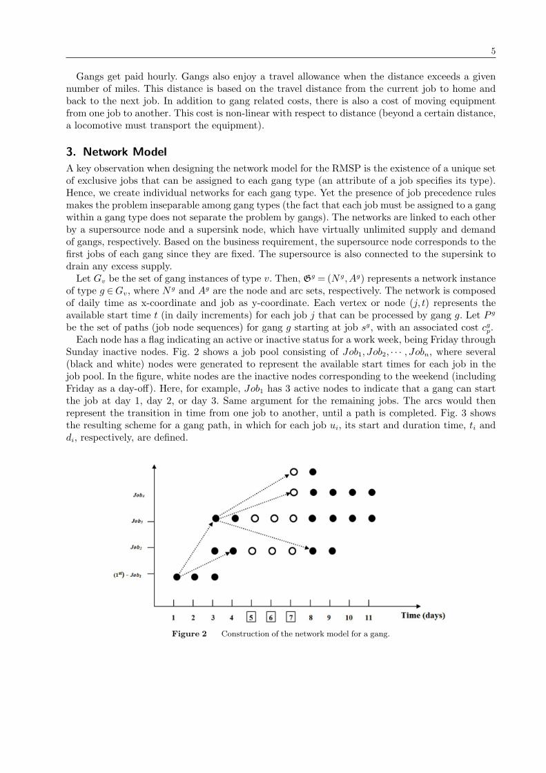
Sunday inactive nodes. Fig. 2 shows a job pool consisting of Job1, Job2, · · · , Jobn, where several(black and white) nodes were generated to represent the available start times for each job in thejob pool. In the figure, white nodes are the inactive nodes corresponding to the weekend (includingFriday as a day-off). Here, for example, Job1 has 3 active nodes to indicate that a gang can startthe job at day 1, day 2, or day 3. Same argument for the remaining jobs. The arcs would thenrepresent the transition in time from one job to another, until a path is completed. Fig. 3 showsthe resulting scheme for a gang path, in which for each job ui, its start and duration time, ti anddi, respectively, are defined.

Figure 2 Construction of the network model for a gang.

6

Figure 3 Scheme of a job-gang path.

Algorithm 1 – Solving RMSP by Alg1

Input: An instance of the RMSP.Step 1: Construct the job-time network for each gang type.Step 2: Find a path for each gang by running a DP-based shortest path algorithm.Step 3: Phase 1: Find an initial solution by starting from solution obtained in Step 2.Step 4: Phase 2: Apply an enhanced solution procedure to the initial point found in Phase 1.

Output: A favorable job-gang schedule for the RMSP.

Concerning arc costs, they are calculated by travel miles and measured in dollar units. This isreferred to the money paid to gangs traveling between the locations of two consecutive jobs. Theformal definition of arc cost is given by: a) Travel costs between the location of job j and thehome-town of the gang if the duration of job j contains weekends; b) travel costs between thelocation of job j and the home-town of the gang, plus the travel cost between the home-town ofthe gang and the location of the next job, if the time span of job j’s end time and the next job’sstart time contains weekends; and c) equipment movement costs from the location of job j to thelocation of the next job.

4. Solution Methodology

In this section, a two-phase heuristic approach is proposed to overcome the inherent complexityand relatively tight delivery date posed by RMSP-instances. Instead of employing a traditionallocal search strategy, we combine very large-scale neighborhood search ideas with mathematicalprogramming. To this end, we develop a two-phase solution procedure. Basically, we construct a job-time network model for each gang type, and obtain a set of gang-paths by applying a shortest pathalgorithm using a dynamic programming method. As a result, the set of job-gang paths obtainedis used in Phase 1 to heuristically assign jobs to gangs in order to find a feasible initial point. APhase 2 is then applied to improve the initial solution by means of mathematical programmingtechniques. A summary of the solution framework is given in Algorithm 1.

The strategic idea behind Algorithm 1 stems from the fact that there is an exclusive job poolwhich can only be processed by gangs of a particular type. This decomposition significantlydecreases the problem size and speeds up the solving time. Furthermore, other business rules suchas job precedence and robustness are also relaxed. We propose two minimal constants, u1 and u2,for the job precedence and robustness rules, respectively. These constants ensure that several strictrules are satisfied while other less important rules can be violated with no or insignificant penalty.Note that the robustness of the solution is nothing but the number of pairs of scheduled jobs locatedwithin a certain distance to each other and are concurrently performed. The full mathematicalmodel is listed in Appendix A.

7

4.1. Phase 1: Finding an initial solution

The first phase of the solution methodology is to find a feasible initial solution to the RMSP. This isaccomplished by a heuristic searching procedure that basically comprises 4 modules, namely inser-tion, swap and increasing flexibility methods and a cycle overcome function, which are discussednext. The flowchart in Fig. 4 depicts Phase 1 of our proposed solution framework.

Figure 4 Solution framework, Phase 1: Finding a feasible initial point.

4.1.1. A DP-based shortest path algorithm

Finding the optimal scheduling for each gang type is similar to find the shortest path with minimalcost in the job-time network. Hence, we apply a shortest path algorithm based on a dynamicprogramming method. Basically, the gang path to be found would cover all the jobs beginning fromthe first job, with a resulting cost being the cumulated cost of the last job node.

Once a gang finishes a job, the starting time for the next job is given by the finished job’send time plus the transition time. Consequently, the finished job’s neighbors are those jobs whoseavailable starting time are later than the calculated finished job’s end time. As shown in Fig. 2, thefirst job (Job1) requires 2 working days to be done. Here, we call the completion day as duration.After finishing Job1, the gang can move to either Job2 or Job3 immediately, or it can wait 4 working

8

days and then move to Job4. Normally, the latter situation is impractical in real-life applications.Hence, only Job1’s neighbors (Job2 and Job3) are considered.

Balanced workload for the same gang type is an important requirement imposed by union reg-ulations. As a strategy to handle this requirement, we do not choose the exact shortest pathwith the maximum number of jobs and smallest cumulated cost at the last job node. Instead wetry to choose a path whose total duration sumDur (jobs completion time) falls in the range of[minWorkingDays,maxWorkingDays], or, [minW,maxW ] for simplicity. By doing so, we avoidviolating several union rules since the shortest path may lead to one gang having a heavy workload,i.e., 250 days per year, while another gang having only 100 working days.

If no such path exits, a penalty cost occurs by incorporating the penalty multiplier (1 + k ∗balancePenalty), with k as a constant, and balancePenalty = sumDur−maxW

maxW−minWif sumDur >maxW

or balancePenalty = minW−sumDurmaxW−minW

if sumDur < minW , i.e., the duration of the path exceedsthe maximal working time or is less than the minimal working time, respectively. The optimalitycondition for choosing a path is to follow the rule that the optimal path should have at least 2/3times the number of jobs that the longest path in the current network has.

4.1.2. Insertion procedure

As mentioned above, several kinds of soft and hard constraints make the problem harder to solve.For example, gangs have a limited amount of working days per year, whereas the available jobshave a restricted time window. In addition, a set of precedence and robustness rules is imposedto certain jobs. Hence, the paths provided by the shortest path algorithm may not be suitable toschedule all possible jobs, thus leading to a pool of unassigned jobs.

To overcome this, the remaining unassigned jobs are inserted in the current paths (i.e., optimalpaths for the corresponding gang types). Here, subsequent assigned jobs are pushed back afterinsertion of unassigned jobs. Fig. 5 shows the insertion procedure of unassigned Job5 in front ofJob3. The optimality condition for the position of insertion is to choose the smallest incrementcost of the path among all possible positions and all possible paths for gangs of the same type. Asan imperative requirement to successfully perform this insertion, the modified path must meet allimposed requirements, including job time windows, precedence rules and robustness.

However, often not all jobs are able to be inserted in the available paths since subsequent jobs have time

Job1 Job2 Job3 Job4

Job5

Job5 Job1 Job2 Job3 Job4

Figure 5 Insertion of unassigned jobs. Unassigned job Job5 is inserted before job Job3.

Due to the very tight time windows of the jobs, the insertion procedure is somehow limited.Pushing back or forward those jobs already assigned to paths may cause violation of such timeconstraints, and thus, several unassigned jobs may remain unassigned after this stage. To overcomethis, in the next section we introduce a swap and extraction method that increases the flexibilityof the current paths to enforce the assignment of all remaining unassigned jobs.

9

4.1.3. Swap method

Since some unassigned jobs may remain in the pool of unassigned jobs after the insertion procedure,we apply a two-stage procedure. First, we strategically create enough room or ‘holes’ in the currentpaths by extracting those assigned jobs that can be swapped for unassigned jobs. Second, we insertthe unassigned jobs and label the recently extracted job as unassigned. The key idea is to interferewith the smallest number of assigned jobs.

Fig. 6 shows the undone Job5 being swapped out for Job3 and Job4, which were previouslyassigned to the path. As a result, Job3 and Job4 become undone jobs.

We design a procedure to determine the positions of swapping jobs, and thus increasing theflexibility of the paths, based on the curRatio function given by:

curRatio =incrementCost × timeWindowLength2 × curNumJobs

timeWindowLength,

where timeWindowLength =∑

in swapped jobs

latestStartTime–earliestStartTime is the sum of time win-

dow length for all jobs that are to be swapped out in the path, and timeWindowLength2 =∑in swapped jobs

latestStartTime–end is the sum of the difference between latest start time and end

time for all jobs that are to be swapped out in the path. The larger the timeWindowLength, themore flexible the jobs are. The smaller the timeWindowLength2, the less flexible the jobs are.

Job5 Job1 Job2

Job3 (unassigned) Job4 (unassigned)

Job5 (unassigned)

Job1 Job2 Job3 Job4

Figure 6 Swap of unassigned and assigned jobs. Unassigned job Job5 replaces jobs Job3 and Job4.

4.1.4. Overcoming the cyclic problem

Running insertion and swap procedures for unassigned jobs lead to the successful insertion of morejobs. However, these procedures may cause the occurrence of cycle problems due to several unas-signed jobs originally inserted in the paths may be swapped out again as the algorithm progresses.This is a result of the inflexibility of the paths observed at the early iterations, i.e., the pathhas many jobs that are scheduled close to their latestStartTime, thus the insertion and swap canhappen only in a few positions. In order to make paths more flexible, a sub-routine called Meet-DueDateJobOut is designed to concurrently extract a set of jobs at random, under the conditionthat the path remains valid and no constraints are violated.

Note that each iteration includes one insertion and one swap. The former largely decreases thenumber of unassigned jobs in the job pool, and the latter slightly increases the number of unassignedjobs in the path. Since the MeetDueDateJobOut sub-routine significantly increases the number ofunassigned jobs, it is run every τ iterations (typically τ=10) until Phase 1 converges.

10

Algorithm 2 – ImprovingStage of Alg1

Input: The initial point provided by Phase 1 of Algorithm 1.Set of job-time networks, predetermined gang paths and data set of unassigned jobs.

Step 0: Iter ← 0repeat

Step 1: Randomly extract assigned jobs from the paths.Step 2: Recombine extracted/uncovered nodes into a pool of subsequences.Step 3: Form and solve an ILP model to optimally create subsequences of nodes.Step 4: Incorporate the optimal solution provided by the reallocation ILP into the currentsolution.Step 5: Iter ← Iter + 1

until Iter ≥ αOutput: An improved gang scheduling for the RMSP.

4.2. Phase 2: An enhanced solution procedure

In this section we propose a more sophisticated procedure that significantly improves the initialsolution found in Phase 1 by covering unassigned jobs.

Since each gang has limited working days for the year and each available job has a restrictedtime window, Phase 1 cannot schedule all the possible jobs. Hence, Phase 2 of the Algorithm 1includes an interchange procedure that iteratively improves the solution by scheduling all the jobsand assuring to find a no worse solution than the initial solution.

The basic idea of Phase 2 is to randomly select certain nodes to be extracted from the startingsolution (see Fig. 7), and then derive sequences of nodes, including extracted nodes and uncoverednodes, to reinsert them into the short-cut solution. Next, we formulate an integer program, andsolve it by applying an ILP solver. The IP-solution is then incorporated back into the originalsolution. This procedure is repeated until an iteration limit is reached or the solution is significantlyimproved. A summary of Phase 2 of the solution framework is given in Algorithm 2.

Figure 7 Points selected for extraction.

11

4.2.1. Extraction

In this step, as shown in Fig. 7, a number of job sequences are extracted randomly from the gangpaths. Basically, we first determine a specific number of job sequences to be extracted from eachgang path. The sequences are composed of a random number of job nodes, and are extracted fromspecific points that are strategically spanned over the whole path. By doing so, we create enoughavailable space (several holes in the path) for the new sequences of job nodes.

Overlapping sequences are permitted for extraction since they basically imply that two or morespecific origin points overlapped when the random number of job nodes of each sequence has beenchosen. In this case, they are treated as a unique entity of nodes.

4.2.2. Recombination

In this step, we use all the extracted and uncovered nodes (see Fig. 8) to create a pool of sub-sequences that can be potentially reinserted into the solution. To make the problem simpler andimprove the performance, we only consider short sequences of nodes. The business rules, such asjob precedence and robustness, are also considered here.

Figure 8 Pool of extracted/uncovered jobs for recombination.

4.2.3. Reallocation Model

In this step, we form an insertion ILP model. By solving the ILP model, we optimally reallocatethe extracted and uncovered nodes from the previous step. Note that the model is always feasiblesince the nodes may always be reinserted back to the original locations. The detailed model isprovided in Appendix A.

We introduce both binary decision variables to indicate whether certain sequences can be insertedat some insertion point i, and integer decision variables to indicate the shifting time of the jobsequences at the short-cut solution after nodes extraction. Note that it is critical to introduce shift-ing time variables since at some insertion point, the starting time of the subsequent job sequencemust be pushed back or forward to, respectively, enlarge or shrink the time window in order toallocate the new sequence of nodes.

Existing approaches to gang scheduling either solve the entire problem directly by an optimiza-tion solver or iteratively over a subset of gangs. Due to the large number of jobs to be scheduledin the real practice, none of the existing approaches are applicable to the problem studied herein.The ILP model is essentially an assignment problem with the additional constraints correspond-ing to job precedence rules, robustness and job time windows, that aims at minimizing the total

12

cost. Since the complete ILP model has a large number of columns, we thus solve it by randomlychoosing a predetermined number of columns from the entire set of columns.

4.2.4. Reinsertion

We incorporate the optimal results obtained from the reallocation ILP model into the solutionusing specially designed insertion operations. This reinsertion step marks the end of an iteration.The entire series of steps will be repeated until a number α of iterations (typically α=5) is reached.

5. Numerical results

The computational results reported herein correspond to a large-scale real-world test case consistingof more than 1,000 jobs, 10–100 gangs with 4 gang types over a 365-day planning horizon. Data,while being supplied by a major Class–1 US railway, are treated with confidentiality and theirdisclosure is somehow limited. The solution procedures were developed in Visual Studio C++v.2008 and run on a 2.4 GHz Intel(R) processor with 2 GByte RAM under MS-Windows operatingsystem.

The purpose of the computational experiments is twofold. First, we evaluate the quality of thegang schedule provided by Algorithm 1 by comparing it to the original schedule performed by thecurrent industry practice. Second, we assess the performance of our heuristic method.

Table 1 shows the comparison analysis between 3 different solutions provided by our heuristic andthe baseline solution currently used by the railway. The only difference among the three solutionsis the weight between the equipment movement cost and the remaining cost components. Foreach corresponding solution type shown in Column 1, the total cost, travel allowance, equipmentmovement (EM) cost and robustness are shown in the subsequent columns. The values correspondto the relative improvement of Alg1-solutions over baseline-solution, which are provided accordinglyfor each concept in Table 1. Soft violations are included in the last column.

Table 1 RI of Alg1-solutions over the baseline-solution.

Total cost Travel allowance EM cost Robustness SoftSolution (%) (%) (%) (%) Violations

A 18.8 22.9 -6.0 34.0 0B 11.1 13.3 -2.4 58.3 0C 5.3 8.1 -12.0 37.8 0

From the results shown in Table 1, we can make three key observations. First, all Alg1-solutionsoutperform the baseline-solution with a relative improvement up to 18.8%, which may result, inmonetary terms, in millions of dollars of annual saving for the railway industry. Second, soft prece-dence rule violations were reduced by 100%. Third, Alg1-solution B achieved the best robustness,yet its total cost is outperformed by Alg1-solution A. Here, a trade off between total cost androbustness may become an important factor for managers to take into account when solving theRMSP.

According to the business requirements, the robustness is a soft rule and we therefore apply apenalty to those jobs that violate it. In general, the larger the robustness penalty, the smaller theviolation will be. However, since the insertion, swap and increase flexibility procedures do not takeinto account any robustness rule, the penalty and number of violations are not exactly negativelycorrelated. Hence, a sensitivity analysis is conducted to evaluate the effect of this penalty on totalcost estimates. Table 2 shows the outcome of conducting such analysis.

13

Table 2 Sensitivity analysis on the robustness of the solution.

Robustness Robustness Soft Total costpenalty violation violation (RI%)

Baseline 1.00 ≥40 –500 0.68 0 11.3%1000 0.65 0 10.1%1500 0.69 0 14.3%2000 0.72 0 6.3%2500 0.69 0 8.6%3000 0.67 0 4.9%

From Table 2, we observe that the best solution achieved by our heuristic is provided by arobustness penalty set to 1500. Here, both total costs and robustness violations were improved bymore than 14% and 30%, respectively, when compared to the baseline solution. More precisely, inrelative terms, robustness rule violations dropped from 1.0 to 0.69, soft precedence rule violationswere reduced by 100%, and total costs were reduced 14.3%.

Several conclusions were drawn based on a more detailed analysis when comparing actual gangschedules provided by our heuristic and the baseline. First, the total duration for gangs of the sametype was similar for both schedules. Second, the divergence of balanced workload for each gang,a very significant issue for the union rules, turned out to be more favorable with our proposedschedule.

Fig. 9 shows the performance of Phase-1 and Phase-2 (P2) of Algorithm 1. From the figure, wecan observe that a significant decrease in the total cost is obtained by Phase-1 (initial solution)when compared to the baseline solution. Similarly, our initial solution is significantly improvedby the first iteration of Algorithm 1’s Phase-2. We observe that total costs keep decreasing untilno significant improvement is achieved after 8 iterations. More precisely, the total cost decreasesrelatively slowly after iteration 3. Concerning the running time, Phase-1 required roughly 1.0 CPU-time hour to provide an initial feasible solution, whereas Phase-2 finished after 8 iterations in about1.5 CPU-time hours. This proves the capability of our heuristic approach when solving RMSP’slarge-scale test cases.

Figure 9 Performance of Phase 1 and Phase 2 of Algorithm 1.

14

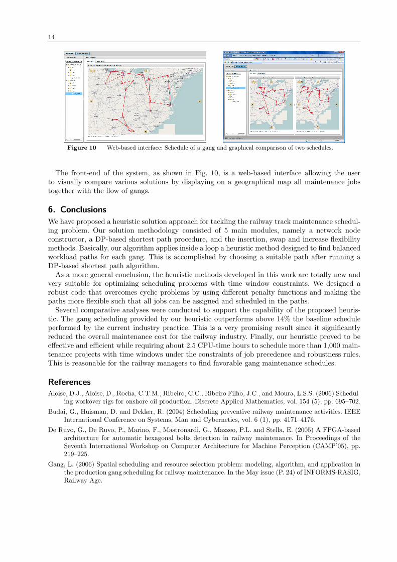
Figure 10 Web-based interface: Schedule of a gang and graphical comparison of two schedules.

The front-end of the system, as shown in Fig. 10, is a web-based interface allowing the userto visually compare various solutions by displaying on a geographical map all maintenance jobstogether with the flow of gangs.

6. Conclusions

We have proposed a heuristic solution approach for tackling the railway track maintenance schedul-ing problem. Our solution methodology consisted of 5 main modules, namely a network nodeconstructor, a DP-based shortest path procedure, and the insertion, swap and increase flexibilitymethods. Basically, our algorithm applies inside a loop a heuristic method designed to find balancedworkload paths for each gang. This is accomplished by choosing a suitable path after running aDP-based shortest path algorithm.

As a more general conclusion, the heuristic methods developed in this work are totally new andvery suitable for optimizing scheduling problems with time window constraints. We designed arobust code that overcomes cyclic problems by using different penalty functions and making thepaths more flexible such that all jobs can be assigned and scheduled in the paths.

Several comparative analyses were conducted to support the capability of the proposed heuris-tic. The gang scheduling provided by our heuristic outperforms above 14% the baseline scheduleperformed by the current industry practice. This is a very promising result since it significantlyreduced the overall maintenance cost for the railway industry. Finally, our heuristic proved to beeffective and efficient while requiring about 2.5 CPU-time hours to schedule more than 1,000 main-tenance projects with time windows under the constraints of job precedence and robustness rules.This is reasonable for the railway managers to find favorable gang maintenance schedules.

ReferencesAloise, D.J., Aloise, D., Rocha, C.T.M., Ribeiro, C.C., Ribeiro Filho, J.C., and Moura, L.S.S. (2006) Schedul-

ing workover rigs for onshore oil production. Discrete Applied Mathematics, vol. 154 (5), pp. 695–702.

Budai, G., Huisman, D. and Dekker, R. (2004) Scheduling preventive railway maintenance activities. IEEEInternational Conference on Systems, Man and Cybernetics, vol. 6 (1), pp. 4171–4176.

De Ruvo, G., De Ruvo, P., Marino, F., Mastronardi, G., Mazzeo, P.L. and Stella, E. (2005) A FPGA-basedarchitecture for automatic hexagonal bolts detection in railway maintenance. In Proceedings of theSeventh International Workshop on Computer Architecture for Machine Perception (CAMP’05), pp.219–225.

Gang, L. (2006) Spatial scheduling and resource selection problem: modeling, algorithm, and application inthe production gang scheduling for railway maintenance. In the May issue (P. 24) of INFORMS-RASIG,Railway Age.

15

Gorman, M.F. and Kanet, J.J. (2010) Formulation and solution approaches to the rail maintenance produc-tion gang scheduling problem. Journal of Transportation Engineering, vol. 136 (8), pp. 701–709.

Higgins, A. (1998) Scheduling of railway track maintenance activities and crews. Journal of the OperationalResearch Society, vol. 49 (10), pp. 1026–1033.

Judge, T. (2010) Railrod still spending for m/w in 2010. January 21. Simmons-Boardman Publishing Corp.(editor) RT&S - Railway Track and Structures.url:http://www.rtands.com/current-issue/railroad-still-spending-for-m-w-in-2010.html

Korgaokar, S. and Mitra, K. (2006) Scheduling supply vessels for an industrial oil exploration operation: amulti-objective evolutionary approach. In Proceedings of International Conference on Industrial Tech-nology, Mumbai, India, pp. 3038–3043.

Lake, M., Ferreira, L. and Murray, M. (2000) Minimizing costs in scheduling railway track maintenance.Computers in Railways VII, Allen, J., Hill, R.J., Brebbia, C.A., Sciutto, G. and Sone, S. (Eds.), Section13: Maintenance and condition monitoring, pp. 895–902, Wessex Institute of Technology Press.

Marino, F., Distante, A., Mazzeo, P.L. and Stella, E. (2007) A real-time visual inspection system for railwaymaintenance: automatic hexagonal-headed bolts detection. IEEE Transactions on Systems, Man, andCybernetics, Part C: Applications and Reviews, vol. 37 (3), pp. 418–428.

Peng, F., Kang, S., Li, X., Ouyang, Y., Somani, K. and Acharya, D. (2011) A heuristic approach to therailroad track maintenance scheduling problem. Computer-Aided Civil and Infrastructure Engineering,vol. 26 (2), pp. 129-145.

Percy, D.F. and Alkali, B.M. (2007) Scheduling preventive maintenance for oil pumps using generalizedproportional intensities models. International Transactions in Operational Research, vol. 14 (6), pp.3038–3043.

Simson, S.A., Ferreira., L. and Murray, M.H. (2000) Rail track maintenance planning: an assessmentmodel. Journal of the Transportation Research Board, Transportation Research Record 1713, NationalAcademy Press, Washington, D.C., pp. 29–35.

Trindade, V. de A. and Ochi, L.S. (2005) Hybrid adaptive memory programming using GRASP and pathrelinking for the scheduling workover rigs for onshore oil production. In Proceedings of Hybrid IntelligentSystems, Rio de Janeiro, Brazil.

Tyagi, T. (2002) Railway track maintenance: role and scope of IT. TATA Consultancy Services, White paper.Transportation Industry Practice.

16

Appendix

A. Reinsertion ILP

We formulate the insertion gang scheduling problem as a network formulation. Given a set of gangs,and a set of jobs to insert, whereby each gang can perform a job in a given amount of time and at agiven cost, the objective is to “attach” each job to an existing path (gang schedule), and timetablethem to minimize total cost. For simplicity, we assume that the duration of jobs is independent ofgangs.

A.1. Nomenclature:

The following notation is defined for each gang type v. As defined in Section 3, a job node isrepresented by (u, t), where u is the job, and t is the starting time. A path p consists of a sequence ofjob nodes, i.e., p≡ {(u1, t1), (u2, t2), · · · , (un, tn)}, with t1 ≤ t2 ≤ · · · ≤ tn and all jobs being different.For path p and time t, we denote by p+ t the path defined by {(u1, t), (u2, t2+ t− t1), · · · , (un, tn+t− t1)}. This entails to managing path p to time t while preserving the job sequence.

Sets and parameters:N : set of all job nodes;F : set of extracted and uncovered job nodes;O: set of job nodes remaining in the network after extraction, O=N −F ;P: set of paths constructed based on extracted/uncovered jobs;I: set of insertion points;fj(p): first job of path p;lj(p): last job of path p;J i: set of starting nodes available for insertion point i;T : total number of working periods (in days);γis: cost due to insertion of path s∈P at insertion point i;

Sim: set of job pairs (u,w) such that it is not desirable for jobs u and w to be processed simulta-neously; u,w ∈N ;Pre: set of job pairs (u,w) such that job u must be processed before job w; u,w ∈N ;Du: duration (days) of job u;sd(p): start time of path p;ed(p): end time of path p;jobs(p): set of jobs associated with path p;tr(u,w): travel time from the location of job u to the location of job w;

Decision variables:We assume that insertion points are ordered in time within each gang. Notation i+1 represents

the insertion point immediately after insertion point i (i and i+1 belong to the same gang). Giveninsertion point i, we call the remaining path at i, denoted as ri, the segment of the original pathbetween insertion points i and i+1, see Fig. 11. In the figure, dotted and solid lines compose thenew path, in which the former may have increased or shrunk, and the latter remain unchanged.Note that the path is shifted in time. In addition, we assume that before insertion point i nochanges have been made to the path. Let also t(p, j), p∈P, j ∈N be sd(p)−time of node j.

We then define 3 types of binary variables:

X is =

{1 if path s∈P is inserted at the insertion point i∈ I0 otherwise.

Y ji =

{1 1 if ri, i∈ I starts at node j0 otherwise.

17

Figure 11 New path after insertion of unassigned/uncovered jobs.

Zuw =

{1 1 if jobs (u,w)∈ Sim are performed at the same time0 otherwise.

A.2. IP model

The mathematical model is formulated as follows:Objective function:

min∑s∈P

∑i∈I

γisX

is

Subject to:Node-sequence assignment: ∑

s:u∈jobs(s)s∈P

∑i∈I

X is = 1,∀u∈F . (1)

Constraint (1) imposes that each extracted/uncovered node belongs to exactly one reconstructedpath s∈P.Insertion constraint: ∑

s∈P

X is ≤ 1,∀i∈ I. (2)

Constraint (2) specifies that no more than one reconstructed path can be inserted at an insertionpoint.Starting point constraint: ∑

j∈J i

Y ij = 1, ∀i∈ I. (3)

Constraint (3) specifies that exactly one starting node is selected for insertion point i.Time constraints:

X is ≤

∑j∈J i

j=(fj(s),t)t≥ed(s)+tr(lj(s),fj(ri))

Y ij ,∀s∈P,∀i∈ I, (4)

Y ij ≤

∑s∈P

sd(s)≥ed(ri+t(ri,j))+tr(lj(ri),fj(s))

X i+1s ,∀j ∈J i,∀i∈ I. (5)

18

Constraint (4) ensures that the starting time of ri, i∈ I must be after the end time of the insertedpath s at insertion point i. Constraint (5) imposes that the inserted path s at the next insertionpoint i+1 must start after the end time of ri and the corresponding travel time.Precedence constraints:∑

s:(u,t)∈ss∈P

∑t≤t1

∑i∈I

X is ≤

∑s:(w,t)∈s

s∈P

∑t≥t1+Du

∑i∈I

X is,∀(u,w)∈ Pre,u,w ∈F ,∀t1 ∈ (0, T ], (6)

∑s:(u,t)∈s

s∈P

∑t≤t1

∑i∈I

X is ≤

∑j∈J i

∑i∈I

(w,t)∈ri+t(ri,j)

∑t≥t1+Du

Y ij ,∀(u,w)∈ Pre,u∈F ,w ∈O,∀t1 ∈ (0, T ], (7)

∑i∈I

(u,t)∈ri+t(ri,j)

∑t≤t1

∑j∈J i

Y ij ≤

∑s:(w,t)∈s

s∈P

∑t≥t1+Du

∑i∈I

X is,∀(u,w)∈ Pre,u∈O,w ∈F ,∀t1 ∈ (0, T ], (8)

∑i∈I

(u,t)∈ri+t(ri,j)

∑t≤t1

∑j∈J i

Y ij ≤

∑i∈I

(w,t)∈ri+t(ri,j)

∑t≥t1+Du

∑j∈J i

Y ij ,∀(u,w)∈ Pre,u,w ∈O,∀t1 ∈ (0, T ]. (9)

Constraints (6)–(9) ensure that job u must be processed before job w for each (u,w)∈ Pre. Forexample, in (6) we impose for each possible time t1, if job u starts before t1, then job w must startafter t1 +Du.Robustness constraints:∑

s:(u,t)∈ss∈P

∑i∈I

X is +

∑s:(w,t)∈s

s∈P

∑i∈I

X is ≤Zuw +1,∀(u,w)∈ Sim,u,w ∈F ,∀t∈ [0, T ], (10)

∑s:(u,t)∈s

s∈P

∑i∈I

X is +

∑i∈I

(w,t)∈ri+t(ri,j)

∑j∈J i

Y ij ≤Zuw +1,∀(u,w)∈ Sim,u∈F ,w ∈O,∀t∈ [0, T ], (11)

∑i∈I

(u,t)∈ri+t(ri,j)

∑j∈J i

Y ij +

∑s:(w,t)∈s

s∈P

∑i∈I

X is ≤Zuw +1,∀(u,w)∈ Sim,u∈O,w ∈F ,∀t∈ [0, T ], (12)

∑i∈I

(u,t)∈ri+t(ri,j)

∑j∈J i

Y ij +

∑i∈I

(w,t)∈ri+t(ri,j)

∑j∈J i

Y ij ≤Zuw +1,∀(u,w)∈ Sim,u,w ∈O,∀t∈ [0, T ], (13)

∑u,w∈Sim

Zuw ≤K. (14)

Constraints (10)–(13) ensure that if jobs u and w are processed at the same time, then Zuw = 1.Since robustness constraints are “soft”, we impose an upper bound (14).

This formulation/notation neglects job time windows and possible other requirements that arestraight forward to incorporate. Soft precedence constraints can easily be derived from (6)–(9) andthe concept presented in (10)–(13).