Strange Attractors: Creating Patterns in Chaos by Julien C....
591
Strange Attractors: Creating Patterns in Chaos by Julien C. Sprott Converted to PDF by Robert Coldwell 8/1/2000 [email protected]
Transcript of Strange Attractors: Creating Patterns in Chaos by Julien C....

Strange Attractors:Creating Patterns in Chaos
byJulien C. Sprott
Converted to PDF by Robert Coldwell8/1/2000

ContentsWhy This Book Is for You
Chapter 1: Order and Chaos1.1 Predictability and Uncertainty1.2 Bucks and Bugs1.3 The Butterfly Effect1.4 The Computer Artist
Chapter 2: Wiggly Lines2.1 More Knobs to Twiddle2.2 Randomness and Pseudorandomness2.3 What’s in a Name?2.4 The Computer Search2.5 Wiggles on Wiggles2.6 Making Music
Chapter 3: Pieces of Planes3.1 Quadratic Map in Two Dimensions3.2 The Butterfly Effect Revisited3.3 Searching the Plane3.4 The Fractal Dimension3.5 Higher-Order Disorder3.6 Strange Attractor Planets3.7 Designer Plaids3.8 Strange Attractors that Don’t3.9 A New Dimension in Sound
Chapter 4: Attractors of Depth4.1 Projections4.2 Shadows4.3 Bands4.4 Colors4.5 Characters4.6 Anaglyphs4.7 Stereo Pairs | Stereo Pairs4.8 Slices
Chapter 5: The Fourth Dimension5.1 Hyperspace5.2 Projections5.3 Other Display Techniques5.4 Writing on the Wall5.5 Murals and Movies5.6 Search and Destroy
4
668
1417
25252628304048
505054567480
107125132142
147147171191208211216222241
259259263288315317318

Chapter 6: Fields and Flows6.1 Beam Me up Scotty!6.2 Professor Lorenz and Dr. Rössler6.3 Finite Differences6.4 Flows in Four Dimensions6.5 Strange Attractors that Aren’t6.6 Doughnuts and Coffee Cups
Chapter 7: Further Fascinating Functions7.1 Steps and Tents7.2 ANDs and ORs7.3 Roots and Powers7.4 Sines and Cosines7.5 Webs and Wreaths7.6 Swings and Springs7.7 Roll Your Own
Chapter 8: Epilogue8.1 How Common is Chaos?8.2 But Is It Art?8.3 Can Computers Critique Art?8.4 What’s Left to Do?8.5 What Good Is It?
Appendix A: Annotated Bibliography
Appendix B: BASICProgram Listing
Appendix C: Other Computers and BASIC VersionsBASICA and GW-BASICTurbo BASICand PowerBASICVisualBASIC for MS-DOSVisualBASIC for WindowsQuickBASICfor Apple Macintosh Systems
Appendix D: C Program Listing
Appendix E: Summary of Equations
Appendix F: Dictionaries of Strange Attractors
322322326329352368384
397397408418428438448459
460460467468470476
480
491
514514514515515521
528
566
576

Why This Book Is for You
Art and science sometimes appear in juxtaposition, one aesthetic, the otheranalytical. This book bridges the two cultures. I have written it for the artist who iswilling to devote a modicum of effort to understanding the mathematical world ofthe scientist and for the scientist who often overlooks the beauty that lurks justbeneath even the simplest equations.
If you are neither artist nor scientist, but own a personal computer for whichyou would like to find an exciting new use, this book is also for you. Fractalsgenerated by computer represent a new art form that anyone can appreciate andappropriate. You don’t have to know mathematics beyond elementary algebra,and you don’t have to be an expert programmer. This book explains a simple, newtechnique for generating a class of fractals called strange attractors. Unlike otherbooks about fractals that teach you to reproduce well-known patterns, this one willlet you produce your own unlimited variety of displays and musical sounds with asingle program. Almost none of the patterns you produce will ever have been seenbefore.
To get the most out of this book, you will need a personal computer, thoughit need not be a fancy one. It should have a monitor capable of displaying graphics,preferably in color. Some knowledge of BASIC is useful, although you can just typein the listings even if you don’t understand them completely. For those of you whoare C programmers, I have provided an appendix with an equivalent version in C.You may find the exercises in this book an enjoyable way to hone your program-ming skills. As you progress through the book, you will gradually develop a verysophisticated computer program. Each step is relatively simple and brings excitingnew things to see and explore. Alternately, you can use the accompanying diskimmediately to begin making your own collection of strange attractors.
4

Strange Attractors
How to find them, those regionsOf space where the equation traces
Over and over a kind of path,Like the moth that batters its way
Back toward the lightOr, hearing the high cry of the bat,
Folds its wings in a rolling dive?
And ourselves, fluttering toward and awayIn a pattern that, given enoughDimensions and point-of-view,
Anyone living there could plainly see—Dance and story, advance, retreat,
A human chaos that some slightEarly difference altered irretrievably?
For one, the sound of her motherCrying. For this other,
The hands that soothedWhen he was sick. For a third,
The silence that collectsAround certain facts. And this one,Sent to bed, longing for a nightlight.
Though we think this time to escape,Holding a head up, nothing wrong,Finding a way to beat the system,
Talking about anything else—Travel, the weather, time
At the flight simulator—for someThe journey circles back
To those strange, unpredictable attractors,Secrets we can neither speak nor leave.
—Robin S. Chapman
5

6
Chapter 1Order and Chaos
This chapter lays the groundwork for everything that follows in the book.Nearly all the essential ideas, mathematical techniques, and programming toolsyou need are developed here. Once you’ve mastered the material in this chapter,the rest of the book is smooth sailing.
1.1 Predictability and Uncertainty
The essence of science is predictability. Halley’s comet will return to thevicinity of Earth in the year 2061. Not only can astronomers predict the very minutewhen the next solar eclipse will occur but also the best vantage point on Earth fromwhich to view it. Scientific theories stand or fall according to whether their predic-tions agree with detailed, quantitative observation. Such successes are possiblebecause most of the basic laws of nature are deterministic, which means they allowus to determine exactly what will happen next from a knowledge of presentconditions.
However, if nature is deterministic, there is no room for free will. Humanbehavior would be predetermined by the arrangements of the molecules thatmake up our brains. Every cloud that forms or flower that grows would be a directand inevitable result of processes set into motion eons ago and over which thereis no possibility for exercising control. Perfect predictability is dull and uninteresting.Such is the philosophical dilemma that often separates the arts from the sciences.
One possible resolution was advanced in the early decades of the 20thcentury when it was discovered that the quantum mechanical laws that govern thebehavior of atoms and their constituents are apparently probabilistic, which meansthey allow us to predict only the probability that something will happen. Quantummechanics has been extremely successful in explaining the submicroscopic world,but it was never fully embraced by some scientists, including Albert Einstein, whountil his dying day insisted that he did not believe that God plays dice with theUniverse.
Since the 1970s science has been undergoing an intellectual revolution thatmay be as significant as the development of quantum mechanics. It is now widelyunderstood that deterministic is not the same as predictable. An example is theweather. The weather is governed by the atmosphere, and the atmosphere obeys

deterministic physical laws. However, long-term weather predictions have im-proved very little as a result of careful, detailed observations and the unleashing ofvast computer resources.
The reason for this unpredictability is that the weather exhibits extremesensitivity to initial conditions. A tiny change in today’s weather (the initial condi-tions) causes a larger change in tomorrow’s weather and an even larger changein the next day’s weather. This sensitivity to initial conditions has been dubbed thebutterfly effect, because it is hypothetically possible for a butterfly flapping its wingsin Brazil to set off tornadoes in Texas. Since we can never know the initial conditionswith perfect precision, long-term prediction is impossible, even when the physicallaws are deterministic and exactly known. It has been shown that the predictabilityhorizon in weather forecasting cannot be more than two or three weeks.
Unpredictable behavior of deterministic systems has been called chaos, andit has captured the imagination of the scientist and nonscientist alike. The word"chaos" was introduced by Tien-Yien Li and James A. Yorke in a 1975 paper entitled"Period Three Implies Chaos." The term "strange attractors," from which this booktakes its title, first appeared in print in a 1971 paper entitled "On the Nature ofTurbulence," by David Ruelle and Floris Takens. Some people prefer the term"chaotic attractor," because what seemed strange when first discovered in 1963 isnow largely understood.
It’s not hard to imagine that if a system is complicated (with many springs andwheels and so forth) and hence governed by complicated mathematical equa-tions, then its behavior might be complicated and unpredictable. What has comeas a surprise to most scientists is that even very simple systems, described by simpleequations, can have chaotic solutions. However, everything is not chaotic. After all,we can make accurate predictions of eclipses and many other things. An evenmore curious fact is that the same system can behave either predictably orchaotically, depending on small changes in a single term of the equations thatdescribe the system. For this reason, chaos theory holds promise for explaining manynatural processes. A stream of water, for example, exhibits smooth (laminar) flowwhen moving slowly and irregular (turbulent) flow when moving more rapidly. Thetransition between the two can be very abrupt. If two sticks are dropped side-by-side into a stream with laminar flow, they stay close together, but if they aredropped into a turbulent stream, they quickly separate.
Chaotic processes are not random; they follow rules, but even simple rulescan produce extreme complexity. This blend of simplicity and unpredictability alsooccurs in music and art. A piece of music that consists of random notes or of anendless repetition of the same sequence of notes would be either disastrously
7
discordant or unbearably boring. Likewise, a work of art produced by throwingpaint at a canvas from a distance or by endlessly replicating a pattern, as inwallpaper, is unlikely to have aesthetic appeal. Nature is full of visual objects, suchas clouds and trees and mountains, as well as sounds, like the cacophony of excitedbirds, that have both structure and variety. The mathematics of chaos provides thetools for creating and describing such objects and sounds.
Chaos theory reconciles our intuitive sense of free will with the deterministiclaws of nature. However, it has an even deeper philosophical ramification. Not onlydo we have freedom to control our actions, but also the sensitivity to initialconditions implies that even our smallest act can drastically alter the course ofhistory, for better or for worse. Like the butterfly flapping its wings, the results of ourbehavior are amplified with each day that passes, eventually producing a com-pletely different world than would have existed in our absence!
1.2 Bucks and Bugs
Enough philosophizing—it’s time to look at a specific example. This examplerequires some mathematics, but the equations are not difficult. The ideas andterminology are important for understanding what is to follow.
Suppose you have some money in a bank account that provides interest,compounded yearly, and that you don’t make any deposits or withdrawals. Let’slet X represent the amount of money in your account. When the time comes for thebank to credit your interest, its computer does so by multiplying X by some number.With an interest rate of 10%, the number is 1.1, and your new balance is 1.1 X. If yourbalance in the nth year is Xn (where n is 1 after the first year, 2 after the second, andso forth), your balance in the year n +1 is
Xn +1 = R Xn (Equation 1A)
where R is equal to 1.0 plus your interest rate. (R is 1.1 in this example.)
You probably know that such compounding leads to exponential growth. Interms of the initial amount X0, the amount in your account after n years is
Xn = X0Rn (Equation 1B)
After 50 years at 10% yearly interest, you will have $117.39 for every dollar youinitially invested. The bank can afford to do this only because of inflation and
8

because money is loaned at an even higher interest rate.
Equation 1A is applicable to more than compound interest. It’s how many ofus have our salaries determined. It also describes population growth. Imagine somespecies of bug that lives for a season, lays its eggs, and then dies (thus avoiding theconfusion of overlapping generations). The next year the eggs hatch, and thenumber of bugs is some constant R times the number in the previous year. If R is lessthan 1, the bugs die out over a number of years; and if R is greater than 1, theirnumber grows exponentially.
You also know that exponential growth cannot go on forever, whether it bebucks in the bank, bugs in the back yard or people on the planet. Eventuallysomething happens, such as the depletion of resources, to slow down or evenreverse growth. Mass starvation, disease, crime, and war are some of the mecha-nisms that limit unbridled human population growth. Thus we need to modifyEquation 1A in some way if it is to model growth patterns in nature more closely.
Perhaps the simplest modification is to multiply the right-hand side of Equa-tion 1A by a term such as (1 - X), whose value approaches 1 as X gets smaller (muchless than 1) but is less than 1 as X increases. Since the population dies abruptly as Xapproaches 1, we must think of X = 1 as representing some large number of dollarsor bugs (say a million or a billion); otherwise we would never get very far! So ourmodified equation, called the logistic equation, is
Xn +1 = R Xn (1 - Xn) (Equation 1C)
Now you’re going to get your first homework assignment. Take your pocketcalculator and start with a small value of X, say 0.1. To reduce the amount of workyou have to do, use a fairly large value of R, say 2, corresponding to a doublingevery year. Run X through Equation 1C a few times and see what happens. Thisprocess is called iteration, and the successive values are called iterates. If you didit right, you should see that X grows rapidly for the first couple of steps, and then itlevels off at a value of 0.5. The first few values should be approximately 0.1, 0.18,0.2952, 0.4161, 0.4859, 0.4996, and 0.5. Compare your results with the unboundedgrowth of Equation 1A.
You might have predicted the above result, if you had thought to set Xn+1equal to Xn in Equation 1C and solved for Xn. This value is called a fixed-pointsolution of the equation, because if X ever has that value, it remains fixed thereforever. Such a fixed-point solution is sometimes called a point attractor, becauseevery initial value of X between 0 and 1 is attracted to the fixed point upon repeatediteration of Equation 1C. Try initial values of X = 0.2 and X = 0.8. A fixed point is also
9

called a critical point, a singular point, or a singularity.
If you’re curious, you might wonder what happens if you start with a value ofX less than 0, such as -0.1, or greater than 1, such as 1.1. You should verify that theiterates are negative and that they get larger and larger, eventually approachingminus infinity. We say that the solution is unbounded and that it attracts to infinity.Thus the values of X = 0 and X = 1 are like a watershed. Between these values thesolution is bounded, and outside these values it is unbounded.
The region between X = 0 and X = 1 is called a basin of attraction becauseit resembles a bathroom basin in which drops of water find their way to the drainfrom wherever they start. X = 0 is also a fixed point, but it is unstable because valueseither slightly above or slightly below zero move away from zero. Such an unstablefixed point is sometimes called a repellor. Chaos can result when two or morerepellors are present; the iterates then bounce back and forth like a baseball runnercaught in a squeeze play.
Equations that exhibit chaos have solutions that are unstable but bounded;the solution never settles down to a fixed value or even to a repeating pattern, butneither does it move off to infinity. Sometimes we say that such equations are linearlyunstable but nonlinearly stable. Small perturbations to the system grow, but thegrowth ceases when the nonlinear terms become important, as eventually theymust. Another way to say it is that the fixed points are locally unstable, but the systemis globally stable. In this case initial conditions are drawn to a special type ofattractor called a strange attractor, which is not a point or even a finite set of pointsbut rather a complicated geometrical object whose properties constitute thesubject of this book.
See what happens if you substitute X = 0 or X = 1 into the logistic equation. Asa check on your calculations, or in case you didn’t do your homework, Table 1-1shows the successive iterates of X for each of the cases we have discussed.
Table 1-1. Iterates of the logistic equation for various initial values of X with R=2
n = 0 n = 1 n = 2 n = 3 n = 4 n = 5 n = 6
0.1 0.18 0.2952 0.4161 0.4859 0.4996 0.5
0.2 0.32 0.4352 0.4916 0.4999 0.5 0.5
0.8 0.32 0.4352 0.4916 0.4999 0.5 0.5
-0.1 -0.22 -0.5368 -1.6499 -8.7442 -170.41 -58421
1.1 -0.22 -0.5368 -1.6499 -8.7442 -170.41 -58421
0.0 0.0 0.0 0.0 0.0 0.0 0.0
1.0 0.0 0.0 0.0 0.0 0.0 0.0
10

An equation, such as the logistic equation, that predicts the next value of aquantity from the previous value is called an iterated map because it is like a roadmap in which each point on the earth is mapped to a corresponding point on apiece of paper. The logistic equation is a one-dimensional map because thevarious X values can be thought of as lying along a straight line that stretches fromminus infinity to plus infinity. Each iteration of the map moves every point along theline to a new position on the line. For the example above with R = 2, all the pointsbetween X = 0 and X = 1 walk toward X = 0.5, where they stop and remain. Otherpoints run faster and faster toward the end of the line that stretches to minus infinity.
The logistic equation is an example of a quadratic iterated map, so calledbecause if you multiply out the right-hand side of Equation 1C, it has not only a linearterm RXn but also a quadratic (squared) term -RXn
2. Quadratic maps arenoninvertable because you can find Xn+1 from Xn, but can’t go backwardbecause there are two values of Xn that produce the same Xn+1, and there is noway of knowing from which it came. For example, Table 1-1 shows that X0 = 0.2 andX0 = 0.8 both produce X1 = 0.32. These are the two roots of the quadratic equationthat you get if you try to solve for Xn in Equation 1C in terms of Xn+1.
The graph of Xn+1 versus Xn is a curve called a parabola. Because aparabola is not a straight line, the map is said to be nonlinear. Chaos and strangeattractors require nonlinearity. The interesting and surprising behavior of nonlineariterated maps is the basis for much of this book.
The first surprising result occurs if you iterate Equation 1C with R = 3.2 and aninitial value of X in the range of 0 to 1. After a few iterations the solution will alternatebetween two values of approximately 0.5130 and 0.7995. This is called a period-2limit cycle. Like the fixed point, the limit cycle is another type of simple attractor. Itis sometimes called a periodic or cyclic attractor.
It’s not hard to see how cyclic behavior might arise in nature. If the populationof beetles grows too large, they deplete the plants on whom they depend for food.With too few plants, the beetles die out, allowing the number of plants to recover,leading to the next cycle of beetle growth, and so forth.
Increase R a bit more to 3.5, and repeat the calculation. The result is a period-4 limit cycle with four values of approximately 0.5009, 0.8750, 0.3828, and 0.8269. Ifyou keep increasing R by ever smaller amounts, the period of the limit cycle doublesrepeatedly, finally reaching chaotic behavior (an infinite period) at about R =3.5699456. This value is sometimes called the Feigenbaum point, after Mitchell J.Feigenbaum, a contemporary mathamatician who discovered many of the inter-esting properties of one-dimensional maps.
11

When chaos occurs, the successive iterates fluctuate in an apparentlyrandom and irreproducible manner. The chaotic behavior persists up to R = 4except for an infinite number of small periodic windows. For R greater than 4, thesolution is unbounded, and the iterates attract rapidly to minus infinity.
The behavior described above can be summarized in a bifurcation diagram,as shown in Figure 1-1, in which the limiting iterated values of the logistic equation,after discarding the first few hundred iterates, are plotted for a range of R from 2 to4. This plot is called the Feigenbaum diagram, and it resembles a tree on its side.("Feigenbaum," appropriately but coincidentally, is German for "fig tree.") You seethe fixed-point solution for R less than 3, the period-doubling route to chaos, and theperiodic windows at large R. The chaotic regions toward the right side of the figureare characterized by values of X that span a wide range and eventually fill theregion densely with points.
Figure 1-1. Bifurcation diagram for the logistic equation, Xn+1 = RXn (1 - Xn)
12

Each period doubling is called a bifurcation because a single solution splitsinto a pair of solutions. These splittings are called pitchfork bifurcations for obviousreasons. Note the period-3 window at about R = 3.84. The period-3 region beginsabruptly when R is increased slightly from within the chaotic region to its left in whatis called a tangent or saddle-node bifurcation. Careful inspection of the period-3window shows that it also undergoes a period-doubling sequence at about R = 3.85.Solutions with every period can be found somewhere between R = 3 and R = 4.
Successive period doublings occur with ever-increasing rapidity as onemoves from left to right in Figure 1-1. The ratio of the width of each region to the widthof the previous region approaches a constant equal to 4.669201660910..., calledthe Feigenbaum number. Even more remarkable is that this number arises in manydifferent chaotic systems in nature as well as in the solutions of equations. Theuniversality of the Feigenbaum number in chaos is reminiscent of the ubiquity of thenumber π in Euclidean geometry.
With R = 4 the solutions occupy the entire interval from X = 0 to X = 1. EventuallyX takes on a value arbitrarily close to any point in that interval (a characteristiccalled topological transitivity). Curiously, however, infinitely many initial values of Xdon’t lead to a chaotic solution even for R = 4. For example X0 = 0.5 and X0 = 0.75lead to unstable fixed points, while X0 = 0.345491... and X0 = 0.904508... produce anunstable period-2 limit cycle. By unstable we mean that if the initial values are wrongby even the slightest amount, successive iterates will wander ever farther away.
Even though there are infinitely many nonchaotic initial values between zeroand one, the chance that you will find one by randomly guessing is negligible. Forevery such value, there are infinitely many others that produce chaos. Such aseemingly paradoxical entity is an example of a Cantor set, named after the 19th-century Russian-born German mathematician Georg Cantor who is often creditedwith developing a mathematically rigorous concept of infinity.
A Cantor set contains infinitely many members (in fact, uncountably infinitelymany), but its members represent a zero fraction of the total! For example, infinitelymany points are required to cover completely the circumference of a circle, but thisnumber of points doesn’t even begin to cover its interior. Such a collection (or set)of points, although infinite in number, is said to comprise a set of measure zero,because the points fill a negligible portion of the plane. An attractor is a set ofmeasure zero, but its basin of attraction has a nonzero measure.
Few people would have guessed that such complexity could arise from suchunderlying simplicity. Furthermore, the logistic equation is only the simplest of anendless variety of equations that can exhibit chaos. It is this dichotomy of simplicity
13

and complexity that makes chaos beautiful to the mathematician and artist alike.In the bifurcation diagram of the logistic equation, we have something withaesthetic appeal, and it came from a simple quadratic equation!
1.3 The Butterfly Effect
If our goal is to seek chaotic behavior in the solution of equations, we needa simple way to test for chaos. For this purpose we use the fact that chaoticprocesses exhibit extreme sensitivity to initial conditions, in contrast to regularprocesses in which different starting points usually converge to the same sequenceof points on a simple attractor.
Suppose we iterate the logistic equation with two initial values of X that differby only a tiny amount. Think of these values as representing two states of theatmosphere that differ only by the flapping of the wings of a butterfly. If successiveiterates are attracted to a fixed point as they are for R = 2, the difference betweenthe two solutions must get smaller and smaller as the fixed point is approached. Asimilar thing happens for a limit cycle. The difference between the two solutions willon average decrease exponentially.
If the solution is chaotic, as is the logistic equation for R = 4, the successiveiterates for the two cases initially on average get farther apart; the differenceusually increases exponentially. If the difference doubles on average with everyiteration, we say the Lyapunov exponent is 1. If it is reduced by half, we say theLyapunov exponent is -1. The name comes from the late-19th-century Russianmathematician Aleksandr M. Lyapunov (sometimes transliterated Liapunov orLjapunov).
You can think of the Lyapunov exponent as the power of 2 by which thedifference between two nearly equal X values changes on average for eachiteration. Thus the difference between the values changes by an average of 2L foreach iteration. If L is negative, the solutions approach one another; if L is positive,we have sensitivity to initial conditions and hence chaos.
One way to detect chaos is to iterate the equation with two nearly equalinitial values and see if, after many iterations, the values are closer together orfarther apart. Another way is to make use of a principle of calculus that says that thedifference in the solutions after one iteration divided by the difference before theiteration, provided the difference is small, is equal to the derivative of the equationfor the map, which for the logistic equation is
14
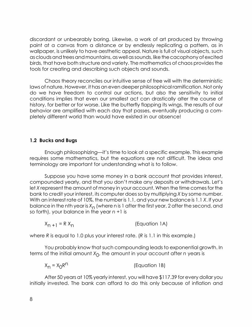
∆Xn+1 / ∆Xn = R(1 - 2Xn) (Equation 1D)
where ∆X is the difference between the two values of X. In Equation 1D, ∆Xn is thedifference in the X values after n iterations, and ∆Xn+1 is the difference after n+1iterations.
Since ∆X increases by the factor on the right of Equation 1D for each iteration,the proper way to calculate the average is to start with a value of 1 and multiply itrepeatedly by the right-hand side of Equation 1D at each iteration, then divide theresult by the number of iterations, and finally take the logarithm to the base 2 of theabsolute value of the result to get the Lyapunov exponent. If you prefer anequation, the preceding description is equivalent to
L = ∑ log2 |R (1 - 2Xn)| / N (Equation 1E)
where the vertical bars mean that you are to disregard the sign of the quantityinside, and ∑ means to sum the quantity to its right from a value of n = 1 to a valueof n = N , where N is some large number. The larger the value of N, the more accuratethe estimate of L.
Suppose you knew the value of X to within 0.01 for an iterated map with L =1. After one iteration the uncertainty would be about 0.02, and after two iterationsthe uncertainty would be about 0.04, and so forth. After about seven iterations, theerror would exceed 1, and your prediction would be totally worthless. If the X valuesare expressed as binary numbers, each iteration would result in throwing away therightmost (least significant) binary digit (bit). Thus the units of L are bits per iteration.Sometimes L is expressed in terms of the natural logarithm (base e) rather than log2.The Lyapunov exponent is the rate at which information is lost when a map isiterated.
It is as if a succession of cartographers each copied maps from one another,but every time one was copied it was only half as accurate as the previous one. Ifthe original map were accurate to 1%, the next copy would be accurate to 2%, andthe seventh generation copy would bear no relation to the original. If the Lyapunovexponent were -1, one bit of information would be gained at each iteration. Evena completely unknown initial condition would eventually be perfectly accurate asit approached the known fixed point or limit cycle. Unfortunately, negative Lyapunovexponents are not the rule in cartography; otherwise all our maps would be self-correcting!
15

Figure 1-2. Lyapunov exponent for the logistic equation
Figure 1-2 shows the Lyapunov exponent for the logistic equation using valuesof R from 2 to 4. The Lyapunov exponent is 1.0 at R = 4 because that value causesthe interval of X from 0 to 1 to be mapped backed onto itself with a single fold atX = 0.5. Thus information is lost at a rate of 1 bit per iteration, because each iteratehas two possible predecessors. You can also see some of the periodic windowswhere L dips below zero toward the right edge of the plot. Also note that L is zerowherever a bifurcation occurs, for example at R=2. At these points the solution isfraught with indecision over which branch to take, and the initial uncertainty persistsforever, neither increasing nor decreasing.
16

1.4 The Computer Artist
By now you have probably surmised that the operations we have describedare best carried out by a computer. The equations are simple, but they must beapplied repeatedly. This is precisely the kind of task at which computers excel.
There are dozens of computer types and programming languages to choosefrom. Currently the most popular computers are those based on the IBM PC runningthe MS-DOS or IBM-DOS operating system (hereafter simply called DOS). The mostwidely available programming language is BASIC (Beginner’s All-purpose SymbolicInstruction Code), which usually comes bundled with the operating system soft-ware included with the computer. A version of BASIC called QBASIC has beenincluded with DOS since version 5.0. BASIC may not be the most advancedcomputer language, but it is one of the easiest to learn and to use, its commandsare close to ordinary English, and it is more than adequate for our purposes.Furthermore, modern versions of BASIC compare favorably with the best of theother languages.
The American National Standards Institute (ANSI) has established a standardfor the BASIC language, but it is somewhat limited, and most versions of BASIC havemany additions and embellishments. We will intentionally use a primitive dialect toensure compatibility with most modern implementations and to simplify the trans-lation into incompatible versions. In particular, the programs in this book should runwithout modification under Microsoft BASICA, GW-BASIC, QBASIC, QuickBASIC,VisualBASIC for MS-DOS; Borland International Turbo BASIC (no longer available);and Spectra Publishing PowerBASIC on IBM PCs or compatibles. You will behappiest using a modern compiled BASIC such as VisualBASIC or PowerBASIC on afast computer with a math coprocessor.
Appendix C includes information on translating the computer programs intoother, partially incompatible dialects of BASIC, as well as source code for use withVisualBASIC for Windows and Microsoft QuickBASIC for the Macintosh. Appendix Dcontains a translation into Microsoft QuickC. The BASIC programs use line numbers,which have been obsolete since the mid-1980s, but they are harmless, and theyprovide a convenient way to reference lines of the program and to indicate wherein the program a change is to be made.
If you follow sequentially through this book, you will need to add and changea only few lines of the program as you meet each new idea. Your program willgradually grow more versatile as you work through the book. In the end you willhave a powerful program that can reproduce all the examples in this book as wellas an endless variety of new ones. Hence you should avoid the temptation to
17

eliminate or to change the line numbers, at least until you have a fully functionalprogram. You may prefer to jump to Appendix B where you will find the completefinal program, which is also provided on the accompanying disk along with sourcelistings in BASIC, Microsoft QuickC, Borland Turbo C++ and a ready-to-run execut-able version of the program.
If you are an experienced programmer, you might ridicule some of the quaintprogram listings. Many powerful programming structures such as block IF state-ments, DO LOOPs, and callable subroutines with local variables that producebeautifully structured programs are now standard, but they have been avoided toallow backwards compatibility with more primitive versions of BASIC. They also oftenimpose a small speed penalty. The dreaded GOTO statement has been usedprimarily to bypass blocks of code in deference to BASIC versions that don’t supportblock IF statements. Lines of the program that are bypassed by a GOTO are usuallyindented. Blocks of the program contained within FOR...NEXT loops have also beenindented. In the interest of structure and simplicity, the programs have been writtenusing numerous small modular subroutines, each with a single entry point beginningwith a comment line, and a single exit point containing a RETURN statement, albeitwith global variables. The individual subroutines are separated with blank lines. Itshould be relatively easy for an experienced programmer to rewrite the programin a more modern format.
The program listing PROG01 iterates the logistic equation for R = 4 with aninitial value of X = 0.05 and makes a graph of each iterate versus its predecessor. Theprogram looks more complicated than it actually is because the various operationshave been relegated to subroutines to provide a template for the more versatilecases to follow.
PROG01. Program for iterating and graphing the logistic equation
1000 REM LOGISTIC EQUATION
1010 DEFDBL A-Z 'Use double precision
1030 SM% = 12 'Assume VGA graphics
1190 GOSUB 1300 'Initialize
1200 GOSUB 1500 'Set parameters
1210 GOSUB 1700 'Iterate equations
18

1220 GOSUB 2100 'Display results
1230 GOSUB 2400 'Test results
1240 ON T% GOTO 1190, 1200, 1210
1250 CLS
1260 END
1300 REM Initialize
1320 SCREEN SM% 'Set graphics mode
1350 WINDOW (-.1, -.1)-(1.1, 1.1)
1360 CLS
1420 RETURN
1500 REM Set parameters
1510 X = .05 'Initial condition
1560 R = 4 'Growth rate
1570 T% = 3
1590 LINE (-.1, -.1)-(1.1, 1.1), , B
1630 RETURN
1700 REM Iterate equations
1720 XNEW = R * X * (1 - X)
2030 RETURN
19

2100 REM Display results
2300 PSET (X, XNEW) 'Plot point on screen
2320 RETURN
2400 REM Test results
2490 IF LEN(INKEY$) THEN T% = 0 'Respond to user key stroke
2510 X = XNEW 'Update value of X
2550 RETURN
If, when you first run the program, your computer reports an error, it is probablyin one of the following lines:
Line 1010: Be sure your version of BASIC supports double-precision (four-byte)floating-point variables. If it doesn’t, you may omit this line, but then you probablywill have to change the 4 in line 1560 to 3.99999 to avoid overflow resulting fromround-off errors. With modern versions of BASIC and a computer with a mathcoprocessor, there is no penalty, and considerable advantage, in using doubleprecision. Because of the finite precision of computer arithmetic, all cases willeventually repeat, but with double precision the average number of iterationsrequired before this happens is acceptably large.
Line 1320: Either your version of BASIC doesn’t require this command or yourcomputer or compiler doesn’t support VGA graphics. Try reducing the 12 in line 1030to a lower number until you find one that works. If none works, try eliminating line1320 altogether.
Line 1350: The WINDOW command defines the coordinates of the lower-leftand upper-right corners of the graphics window for subsequent PSET and LINEcommands. If your version of BASIC doesn’t support this command, you must deletethis line and convert all the parameters in the PSET and LINE commands to addressscreen pixels. In this case try replacing line 2300 with PSET (200 * X, 200 - 200 * XNEW).One advantage of using the WINDOW command is that when a version of BASICcomes along that supports higher screen resolutions, the program can be easilyrecompiled to take advantage of it.
20

Other errors: Look carefully for typographical errors, or consult your BASICmanual to determine compatibility.
The correct program should produce a plot of the logistic parabola, as shownin Figure 1-3. Try different initial values of X (line 1510) and different values of R (line1560) to confirm the behavior predicted for the logistic equation.
Figure 1-3. The logistic parabola from PROG01
The logistic parabola comes from a chaotic solution, but it doesn’t look verycomplicated, and it would hardly qualify as art. With one small change we canmake things more interesting and, at the same time, illustrate sensitivity to initialconditions. Instead of plotting each iterate versus its immediate predecessor, wecould plot it versus its second or third or fourth predecessor. Let’s save the last 500iterates and provide the option to plot X versus any one of them.
21

The changes that you need to make in the program PROG01 to accomplishthis are shown in the listing PROG02. You can either go through the program andchange or add lines as necessary or type the listing and save it in ASCII format andthen use the MERGE command supported by many (mostly old) versions of BASICto update the previous version of the program.
PROG02. Changes required in PROG01 to plot the fifth previous iterate
1000 REM LOGISTIC EQUATION (5th Previous Iterate)
1020 DIM XS(499)
1040 PREV% = 5 'Plot versus fifth previous iterate
1580 P% = 0
2210 XS(P%) = X
2220 P% = (P% + 1) MOD 500
2230 I% = (P% + 500 - PREV%) MOD 500
2300 PSET (XS(I%), XNEW) 'Plot point on screen
If you set PREV% = 1 in line 1040, the result is the same as for PROG01. However,if you set PREV% equal to 2, you see the logistic parabola change into a curve withtwo humps. Each time you increase PREV% by 1, you double the number of humpsin the curve. Thus PREV% = 5 results in 16 oscillations, as shown in Figure 1-4.
22

Figure 1-4. The logistic parabola after five iterations from PROG02
Figure 1-4 provides a good graphical illustration of the sensitivity to initialconditions. The horizontal axis represents all possible initial conditions from zero toone. The vertical axis shows the value from zero to one corresponding to each initialcondition after five iterations. It’s not hard to see that two nearby points on thehorizontal axis usually translate into two very different values along the vertical axisafter five iterations. Try using PREV% = 10, and convince yourself that informationabout the initial condition is almost completely lost after ten iterations.
This exercise provides a good insight into the way a strange attractor isformed geometrically. The logistic parabola, which began as a line (a one-dimensional object), is stretched and folded with each iteration, eventually fillingthe entire plane (a two-dimensional object) after many iterations. Perhaps itreminds you of those taffy machines that repeatedly stretch and fold the taffy,causing two nearby specks in the taffy after a while to be nowhere near one
23

another. On average the distance between the specks initially increases at anexponential rate.
You should be able to think of many other examples of sensitivity to initialconditions. When you stir your coffee to mix in the cream, you’re relying on achaotic process. Two sticks dropped into the water close together just above awaterfall eventually end up far apart. Try laying two identical garden hoses side byside, and turn on the water in each one at the same time without holding the ends.Chaotic processes are all around us. Their mathematical solutions usually producechaotic strange attractors, whose diversity and beauty we are about to explore.
24

Chapter 2Wiggly Lines
In this chapter we will teach the computer to search for chaotic solutions ofsimple equations with a single variable. The solutions are segments of lines, but thelines can wiggle in an incredibly complicated manner.
2.1 More Knobs to Twiddle
The logistic equation (Equation 1C) is an example of a dynamical system.Such systems are described by deterministic initial-value equations. This particularsystem has a single parameter R whose value determines the solution’s behavior forall initial values of X within the basin of attraction. This parameter is like a knob on aradio or on a stove that you can turn up or down to control the sound emitted bythe radio or the convection in a pot of boiling soup.
You can do a simple experiment to observe the period-doubling route tochaos. Go into your bathroom or kitchen and turn on the tap, only slightly, toproduce a regular periodic pattern of drips. Now slowly open the tap until thepattern becomes chaotic. Just before the onset of chaos, if you are sufficientlycareful and patient, you should observe one or more period doublings where thesound changes to something like "drip drip—drip drip—drip drip." The knob thatcontrols the flow rate corresponds to the parameter R in the logistic equation. Thedripping faucet has been extensively studied by Robert Shaw and discussed atlength in his book The Dripping Faucet as a Model Chaotic System.
Usually a dynamical system has more than one knob. Your kitchen faucetprobably has independent control of the flow rate and the temperature of thewater. With more knobs, you might expect to increase the variety of ways thesystem can behave. Such knobs are called control parameters.
The formula for the most general one-dimensional quadratic iterated map is
Xn+1 = a1 + a2Xn + a3Xn2 (Equation 2A)
where a1, a2, and a3 are three control parameters. By exploring all combinationsof their values, we expect eventually to observe every possible peculiar solutionthat the equation can have.
25

You might think that the initial condition X0 is a fourth knob, but if the systemis chaotic, the solution is generally a strange attractor, and all initial conditions withinthe basin of attraction look the same after many iterations. Of course there is noguarantee that a particular choice of X0 lies within the basin, but values of X0 closeto zero are within the basin about half the time, and there are so many chaoticsolutions over the range of the other three parameters that we can well afford todiscard half of them.
The search for strange attractors proceeds as follows. Choose values for a1,a2, and a3 arbitrarily. Start with a value of X0 near zero. Iterate Equation 2Arepeatedly until the solution either exceeds some large number, in which case it ispresumably unbounded, or until the Lyapunov exponent becomes small or nega-tive, in which case the solution is probably a fixed point or limit cycle. In either event,choose a different combination of a1, a2, and a3, and start over. If, after a fewthousand iterations, the solution is bounded (X is not enormous) and the Lyapunovexponent is positive, then it is likely that you have found a strange attractor.
2.2 Randomness and Pseudorandomness
To choose values of a1, a2, and a3, we can use the random-numbergenerator provided with most computer languages. The random numbers thusproduced are usually uniformly distributed between zero and one. You maywonder how a computer, the epitome of determinism, could ever produce arandom number. This question deserves a digression because the answer providesyet another example of the very issues we have been discussing.
One way to produce a random number is to start with a value of X (the seed)between zero and one and iterate the logistic equation with R = 4 a few dozentimes. The result is a new number in the range of zero to one that is related to theseed in a complicated and sensitive way. This number is then used as the seed forthe next random number, which is produced in the same way. A given seed willproduce the same sequence of random numbers, but the sequence may not bethe same on different computers or with different languages or even with differentversions of the same language because of the way the numbers are rounded.
However, this method of producing random numbers is not optimal. First, thenumbers are not uniformly distributed over the range. They tend to cluster near zeroand one as the darkness of the right-hand side of Figure 1-1 suggests. Also,multiplying a non-integer number by itself many times is a relatively slow process ona computer.
26
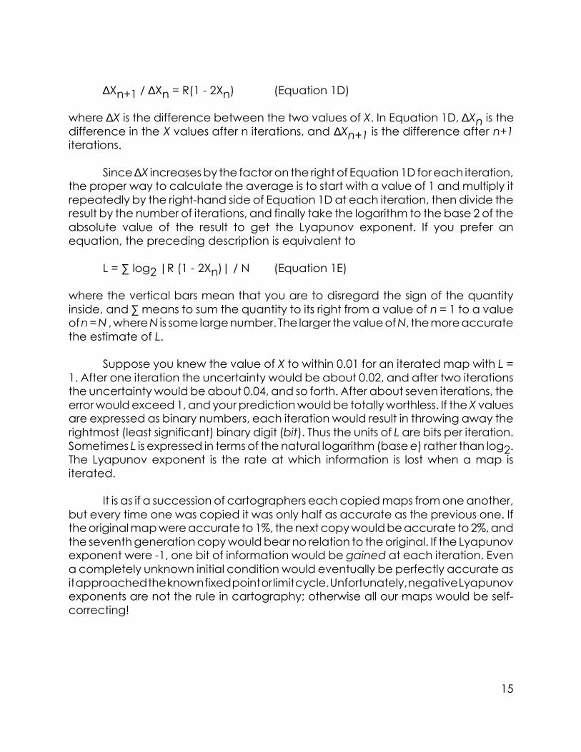
Instead, computers usually get their random numbers using the linearcongruential method:
Xn+1 = (aXn + b) mod c (Equation 2B)
In the mod (modulus) operation, the quantity to the left of the mod (aXn + b)is divided by the quantity to its right (c), and the remainder is kept rather than thequotient. All the quantities in Equation 2B are integers. The constants a, b, and c arecarefully chosen to maximize the number of steps required for the sequence torepeat, which in any case can never exceed c. The numbers are uniformlydistributed from zero to c - 1, but they can be transformed to the range zero to oneby simply dividing Xn+1 by c. The numbers appear to be random, but since they areproduced using a deterministic procedure, they are often called pseudorandom.Equation 2B is another example of a one-dimensional chaotic map, which is relatedto the shift map.
Truly random numbers should satisfy infinitely many conditions. Not only mustthe numbers be uniform over the interval, but there should be no detectablerelation between the numbers and any of their predecessors. In particular, thesequence should repeat only after a very large number of steps. Most random-number generators are deficient in certain ways. For example, the random num-bers produced by Microsoft QBASIC 1.0, QuickBASIC 4.5, and VisualBASIC for DOS1.0 repeat after 16,777,216 steps, and this number is too small for some of ourpurposes.
The situation can be greatly improved by shuffling the numbers. Suppose wemaintain a table of a hundred or so random numbers. When we want one, werandomly take an entry from the table and replace it with a new random number.With this simple modification, the pseudorandom numbers generated by thecomputer are sufficiently random for our purpose.
You should always remember that the sequence of random numbers gener-ated by a digital computer will eventually repeat. You must take care to ensure thatover the duration of a calculation, such a repetition does not occur. You must alsoreseed the random-number generator using a truly random seed, such as onebased on the time of day the program is started, if you are to avoid repeating thesame sequence each time you run the program.
27

2.3 What’s in a Name?
When we begin to choose random values for the coefficients a1, a2, and a3,we are immediately confronted with two issues. The first is the range of values thatthe coefficients may have, and the second is the amount by which two values ofa coefficient must differ to produce attractors that are visibly different.
We can address the first issue by referring to the logistic equation (Equation1C). When the value of R is too small (less than about 3.5), there are no chaoticsolutions, and when the value of R is too large (greater than 4), all the solutions areunbounded. A similar situation occurs for the more general one-dimensionalquadratic map in Equation 2A. Thus we want to limit the coefficients to valueswhose magnitudes (positive or negative) are of order unity. That is, 0.1 is probablytoo small a value and 10 is probably unnecessarily large. This assumption can beverified by numerical experiment.
The second issue requires a subjective judgment of how dissimilar twoattractors must look before we consider them to be different. In practice, a changein one of the coefficients by an amount of order 0.1 generally produces an objectthat is noticeably different. If we let each coefficient take on values ranging from-1.2 to 1.2 in steps of 0.1, we will have 25 possible values. We can associate each witha letter of the alphabet, A through Y, and have a convenient way to catalog andreplicate the attractors. Limiting the coefficients to 25 values may seem excessivelyrestrictive, but since there are three coefficients for one-dimensional quadraticmaps, there are 253 or 15,625 different combinations.
The coefficients that correspond to the logistic equation with R = 4 are a1 =0, a2 = 4, and a3 = -4, and they fall outside the range of -1.2 to 1.2. Thus for somepurposes, it is convenient to take a larger range. A convenient way to extend therange is to use the ASCII (American Standard Code for Information Interchange)character set summarized in Table 2-1.
Table 2-1. ASCII character set and associated coefficient values
Char Dec Coeff Char Dec Coeff Char Dec Coeff
32 -4.5 # 64 -1.3 ` 96 1.9
! 33 -4.4 A 65 -1.2 a 97 2.0
" 34 -4.3 B 66 -1.1 b 98 2.1
28

Char Dec Coeff Char Dec Coeff Char Dec Coeff
# 35 -4.2 C 67 -1.0 c 99 2.2
$ 36 -4.1 D 68 -0.9 d 100 2.3
% 37 -4.0 E 69 -0.8 e 101 2.4
& 38 -3.9 F 70 -0.7 f 102 2.5
‘ 39 -3.8 G 71 -0.6 g 103 2.6
( 40 -3.7 H 72 -0.5 h 104 2.7
) 41 -3.6 I 73 -0.4 i 105 2.8
* 42 -3.5 J 74 -0.3 j 106 2.9
+ 43 -3.4 K 75 -0.2 k 107 3.0
, 44 -3.3 L 76 -0.1 l 108 3.1
- 45 -3.2 M 77 0.0 m 109 3.2
. 46 -3.1 N 78 0.1 n 110 3.3
/ 47 -3.0 O 79 0.2 o 111 3.4
0 48 -2.9 P 80 0.3 p 112 3.5
1 49 -2.8 Q 81 0.4 q 113 3.6
2 50 -2.7 R 82 0.5 r 114 3.7
3 51 -2.6 S 83 0.6 s 115 3.8
4 52 -2.5 T 84 0.7 t 116 3.9
5 53 -2.4 U 85 0.8 u 117 4.0
6 54 -2.3 V 86 0.9 v 118 4.1
7 55 -2.2 W 87 1.0 w 119 4.2
8 56 -2.1 X 88 1.1 x 120 4.3
29

Char Dec Coeff Char Dec Coeff Char Dec Coeff
9 57 -2.0 Y 89 1.2 y 121 4.4
: 58 -1.9 Z 90 1.3 z 122 4.5
; 59 -1.8 [ 91 1.4 { 123 4.6
< 60 -1.7 \ 92 1.5 | 124 4.7
= 61 -1.6 ] 93 1.6 } 125 4.8
> 62 -1.5 ^ 94 1.7 ~ 126 4.9
? 63 -1.4 _ 95 1.8 _ 127 5.0
ASCII codes from 0 to 31 are reserved for control codes—things like back-space, carriage return, and line feed. Codes from 128 to 255 can also be used, butthere is no universal character set associated with them. By making use of all theASCII characters from 0 to 255, we can accommodate coefficients in the range of-7.7 to 17.8. The characters listed in the table will suffice for most of our needs,however.
With such a coding scheme, we can represent each attractor by a sequenceof characters, with each character corresponding to one of the coefficients. Thesequence can be thought of as the name of the attractor. We preface the namewith a character that indicates the type of equation. Let’s use the letter A torepresent one-dimensional quadratic maps. Thus the logistic equation coded in thisway is AMu%. Note that the letters in the name are case sensitive (u and U aredifferent), so you should be careful when typing them. Such names may lookstrange, which is perhaps appropriate for strange attractors, and you shouldn’t tryto pronounce them! However, they do provide a convenient and compactmethod for saving everything you need to reproduce an attractor.
2.4 The Computer Search
Before embarking on a search for strange attractors, we need to generalizethe formula given in Equation 1E for the Lyapunov exponent of the logistic equation.The generalization is easily obtained using differential calculus, and the result is
30

L = ∑ log2 |a2 + 2a3Xn| / N (Equation 2C)
The program changes that are required to perform a search for strangeattractors in one-dimensional quadratic iterated maps are given in the listingPROG03.
PROG03. Changes required in PROG02 to search for strange attractors in one-dimensional qua-dratic maps
1000 REM ONE-D MAP SEARCH
1020 DIM XS(499), A(504), V(99)
1050 NMAX = 11000 'Maximum number of iterations
1160 RANDOMIZE TIMER 'Reseed random-number generator
1360 CLS : LOCATE 13, 34: PRINT "Searching..."
1560 GOSUB 2600 'Get coefficients
1580 P% = 0: LSUM = 0: N = 0: NL = 0
1590 XMIN = 1000000!: XMAX = -XMIN
1720 XNEW = A(1) + (A(2) + A(3) * X) * X
2020 N = N + 1
2110 IF N < 100 OR N > 1000 THEN GOTO 2200
2120 IF X < XMIN THEN XMIN = X
2130 IF X > XMAX THEN XMAX = X
31

2140 YMIN = XMIN: YMAX = XMAX
2200 IF N = 1000 THEN GOSUB 3100 'Resize the screen
2250 IF N < 1000 OR XS(I%) <= XL OR XS(I%) >= XH OR XNEW <= XL OR XNEW >= XH THENGOTO 2320
2410 IF ABS(XNEW) > 1000000! THEN T% = 2 'Unbounded
2430 GOSUB 2900 'Calculate Lyapunov exponent
2460 IF N >= NMAX THEN T% = 2 'Strange attractor found
2470 IF ABS(XNEW - X) < .000001 THEN T% = 2 'Fixed point
2480 IF N > 100 AND L < .005 THEN T% = 2 'Limit cycle
2600 REM Get coefficients
2660 CODE$ = "A"
2680 M% = 3
2690 FOR I% = 1 TO M% 'Construct CODE$
2700 GOSUB 2800 'Shuffle random numbers
2710 CODE$ = CODE$ + CHR$(65 + INT(25 * RAN))
2720 NEXT I%
2730 FOR I% = 1 TO M% 'Convert CODE$ to coefficient values
2740 A(I%) = (ASC(MID$(CODE$, I% + 1, 1)) - 77) / 10
2750 NEXT I%
2760 RETURN
2800 REM Shuffle random numbers
32

2810 IF V(0) = 0 THEN FOR J% = 0 TO 99: V(J%) = RND: NEXT J%
2820 J% = INT(100 * RAN)
2830 RAN = V(J%)
2840 V(J%) = RND
2850 RETURN
2900 REM Calculate Lyapunov exponent
2910 DF = ABS(A(2) + 2 * A(3) * X)
3030 IF DF > 0 THEN LSUM = LSUM + LOG(DF): NL = NL + 1
3040 L = .721347 * LSUM / NL
3070 RETURN
3100 REM Resize the screen
3120 IF XMAX - XMIN < .000001 THEN XMIN = XMIN - .0000005: XMAX = XMAX + .0000005
3130 IF YMAX - YMIN < .000001 THEN YMIN = YMIN - .0000005: YMAX = YMAX + .0000005
3160 MX = .1 * (XMAX - XMIN): MY = .1 * (YMAX - YMIN)
3170 XL = XMIN - MX: XH = XMAX + MX: YL = YMIN - MY: YH = YMAX + MY
3180 WINDOW (XL, YL)-(XH, YH): CLS
3310 LINE (XL, YL)-(XH, YH), , B
3460 RETURN
Here are six points to note about PROG03:
1. The maximum number of iterations (NMAX in line 1050) has been set
33

arbitrarily to 11,000. This is the number of iterations after which a strangeattractor is assumed to have been found if the magnitude of X neverexceeded one million and the Lyapunov exponent is positive (actuallygreater than 0.005). You can decrease NMAX to speed the rate at whichattractors are found, or you can increase NMAX if you have a very fastcomputer or want to give the displays more time to develop. The number ofiterations is a parameter that you can adjust for the most visually appealingresult. Most of the figures in this book were made with NMAX set at betweenabout 500,000 and 10 million, and they required between about a minuteand an hour to produce.
2. The seed for the random-number generator is taken in line 1160 as thenumber of seconds lapsed since midnight (TIMER). This choice ensures that anew sequence of random numbers is produced each time the program isrun, except in the unlikely event that it is run at exactly the same time eachday.
3. After 1000 iterations (line 2200), the screen is resized and erased by thesubroutine in lines 3100 through 3460 using the minimum and maximumvalues of X between the 100th and 1000th iteration, allowing a 10% borderaround the attractor.
4. To save time, the difference between each value of X and its predecessoris evaluated in line 2470, and if the difference is less than one millionth, thesolution is assumed to be a fixed point even if the Lyapunov exponent is stillpositive.
5. The Lyapunov exponent is not used as a criterion until after 100 iterations(line 2480) to ensure that its value is reasonably accurate.
6. The coefficients of the equation are chosen in line 2710 using randomnumbers that have been shuffled by the subroutine in lines 2800 through 2850to minimize the chance of repeating the same search sequence.
The criterion for detecting a strange attractor is somewhat subjective. Therewill always be borderline cases for which no amount of computing will suffice todistinguish between a strange attractor and a periodic solution with a very longperiod. However, our interest here is in finding visually interesting attractors quickly,and so we can afford to make occasional mistakes. Such mistakes account for onlya small fraction of cases.
34

Of the 15,625 combinations of coefficients, exactly 364 (2.3%) are chaotic bythese criteria. Some of the more visually interesting ones are shown in Figures 2-1through 2-4, in which the values are plotted versus their fifth previous iterate. Foreach case, the code and the Lyapunov exponent are shown at the top of thegraph.
Figure 2-1. One-dimensional quadratic map
35

Figure 2-2. One-dimensional quadratic map
36
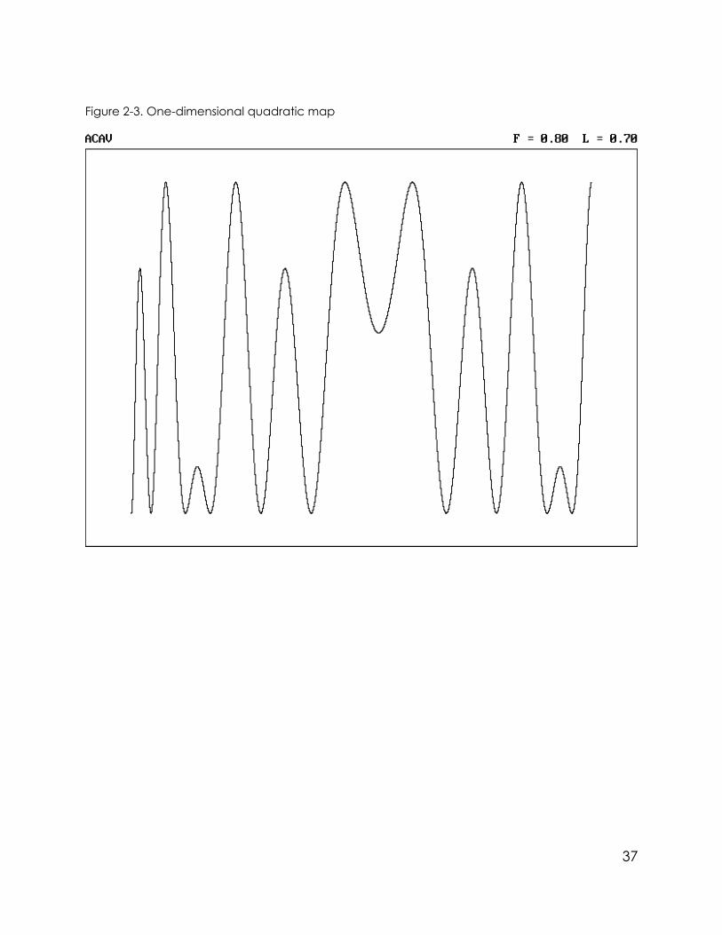
Figure 2-3. One-dimensional quadratic map
37
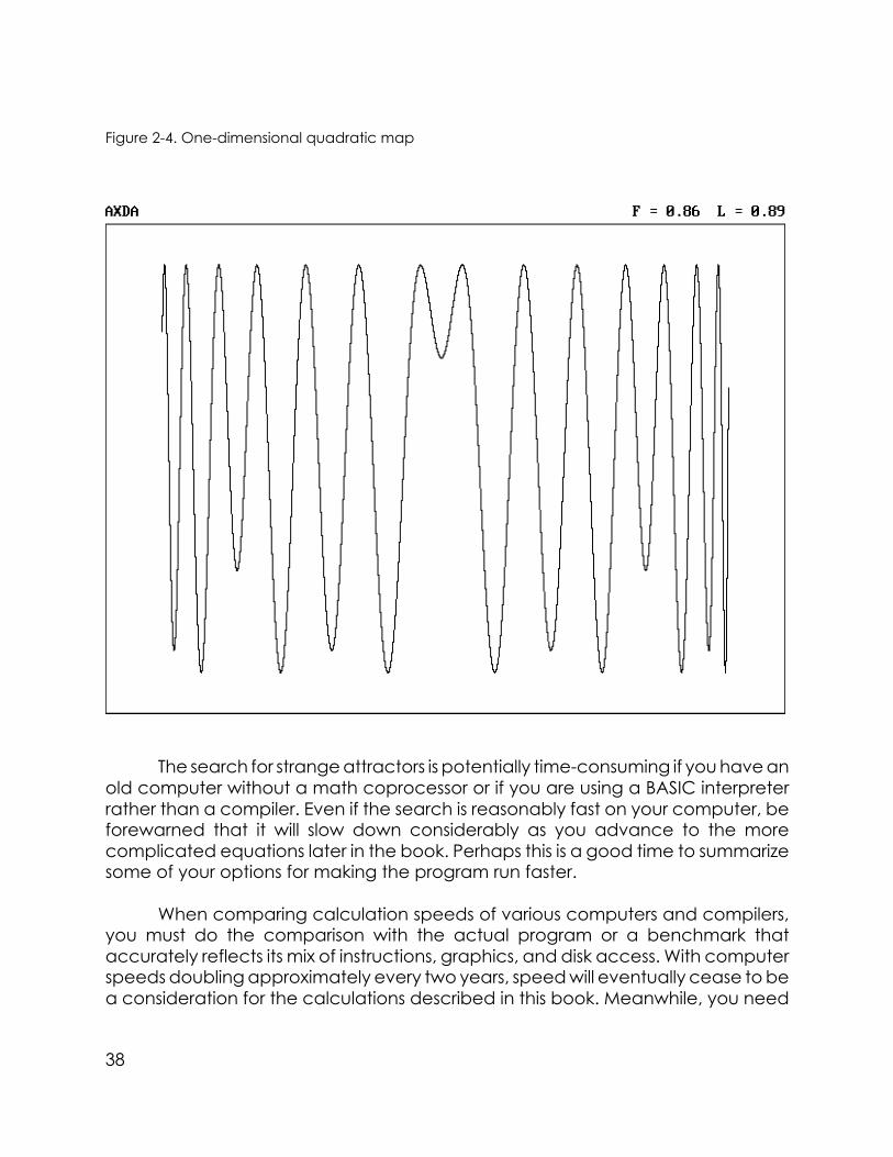
Figure 2-4. One-dimensional quadratic map
The search for strange attractors is potentially time-consuming if you have anold computer without a math coprocessor or if you are using a BASIC interpreterrather than a compiler. Even if the search is reasonably fast on your computer, beforewarned that it will slow down considerably as you advance to the morecomplicated equations later in the book. Perhaps this is a good time to summarizesome of your options for making the program run faster.
When comparing calculation speeds of various computers and compilers,you must do the comparison with the actual program or a benchmark thataccurately reflects its mix of instructions, graphics, and disk access. With computerspeeds doubling approximately every two years, speed will eventually cease to bea consideration for the calculations described in this book. Meanwhile, you need
38

to consider the alternatives.
Table 2-2 lists the average number of strange attractors found by PROG03 perhour using various versions of BASIC on a 33-MHz 80486DX-based computer withand without a math coprocessor. The exact numbers are less important than therelative values. They provide a good indication of how the various versions of BASICcompare on calculations of the type that are used throughout this book.
Table 2-2. Strange attractors found per hour by PROG03 with various versions of BASIC
Publisher Program Ver Type Attractors/hour
No copro Coproc
Microsoft GW-BASIC 3.2 Interpreter 92 92
Microsoft QBASIC 1.0 Interpreter 73 73
Microsoft QuickBASIC 4.5 Interpreter 78 396
Microsoft QuickBASIC 4.5 Compiler 98 390
Microsoft VB for DOS 1.0 Interpreter 72 393
Microsoft VB for DOS 1.0 Comp (alternate) 315 316
Microsoft VB for DOS 1.0 Comp (emulate) 139 418
Borland Turbo BASIC 1.1 Compiler 96 400
Spectra PowerBASIC 3.0 Comp (procedure) 246 1419
Spectra PowerBASIC 3.0 Comp (emulate) 123 1683
QuickBASIC and VisualBASIC for MS-DOS can be run from the editor environ-ment, where they function much like an interpreter, or they can be used to compilea stand-alone executable program. VisualBASIC can be compiled with either oftwo floating point math packages; the alternate package is faster for machineswithout a coprocessor, and the emulate package is faster for machines with acoprocessor. Turbo BASIC is now obsolete and has been replaced by PowerBASIC.
39

PowerBASIC, like VisualBASIC, can be compiled with either of two floating pointmath packages; the procedure package is similar to the VisualBASIC alternatepackage. A third math package, NPX (87) is the same as emulate, except it cannotwork on a machine without a math coprocessor. The tests were done with all errortrapping turned off, which is inadvisable until you have a thoroughly debuggedprogram.
If you launch the program from Microsoft Windows, you might find thecomputation speeds considerably different from those in Table 2.2. In one test, thePowerBASIC speeds were cut in half, and the QuickBASIC speeds were increasedslightly from the values obtained when the program was run directly from DOS. Youshould do your own speed tests to see what configuration provides the optimumperformance on your computer and operating system.
The executable program on the disk that accompanies this book wascompiled with PowerBASIC using the procedure package. If you have PowerBASICand a math coprocessor, you can recompile the program using the emulate or NPX(87) package to achieve a slight improvement in speed.
2.5 Wiggles on Wiggles
The preceding figures consist of segments of wiggly lines, so they are not veryartistic. To make things more interesting, we can consider one-dimensional maps ofhigher order. By this we mean that we will not stop with quadratic (X2) maps, but wewill consider equations containing cubic (X3), quartic (X4), quintic (X5), and evenhigher terms.
In one sense, considering higher-order terms is equivalent to plotting eachiterate versus an iterate earlier than the immediately previous one. For example,two successive iterations of the second-order Equation 2A yields
Xn+2 = a1(1+a2+a1a3) + (a3a2+2a1a3)Xn
+ a3(a2+2a1a3+a22)Xn
2 + 2a2a32Xn
3 + a33Xn
4 (Equation 2D)
which is a fourth-order polynomial. However, there are only three parameters—a1,a2, and a3—from which the five coefficients are uniquely determined.
A simpler and more general procedure is to allow each term in the polyno-mial to have its own coefficient, which for fifth order gives
40

Xn+1 = a1 + a2Xn + a3Xn2 + a4Xn
3 + a5Xn4 + a6Xn
5 (Equation 2E)
With six coefficients, each with 25 possible values, there are 256 or about 244million different combinations. Even if only a small percentage of them is chaotic,we would have to look at one every second for about a year before we would seethem all.
The generalization of the expression for the Lyapunov exponent for a fifth-order map is given by
L = ∑ log2 |a2 + 2a3Xn + 3a4Xn2 + 4a5Xn
3 + 5a6Xn4| / N (Equation 2C)
With these equations in hand, we can easily modify the program in PROG04to search for one-dimensional attractors of up to fifth order. In our coding scheme,a first letter of B represents third order, C represents fourth order, and D representsfifth order. The program is written so that even higher orders can be produced bychanging the quantity OMAX% in line 1060.
PROG04. Changes required in PROG03 to search for strange attractors in one-dimensional maps oforder up to OMAX%
1000 REM ONE-D MAP SEARCH (Polynomials up to 5th Order)
1060 OMAX% = 5 'Maximum order of polynomial
1720 XNEW = A(O% + 1)
1730 FOR I% = O% TO 1 STEP -1
1830 XNEW = A(I%) + XNEW * X
1930 NEXT I%
2650 O% = 2 + INT((OMAX% - 1) * RND)
2660 CODE$ = CHR$(63 + O%)
2680 M% = O% + 1
41

2910 DF = 0
2930 FOR I% = O% TO 1 STEP -1
2940 DF = I% * A(I% + 1) + DF * X
2970 NEXT I%
3000 DF = ABS(DF)
PROG04 produces an interesting array of shapes, samples of which areshown in Figures 2-5 through 2-10. The objects are still segments of lines, but thewiggles themselves have wiggles, and the underlying determinism is less obviousthan before.
Figure 2-5. One-dimensional cubic map
42

Figure 2-6. One-dimensional quartic map
43
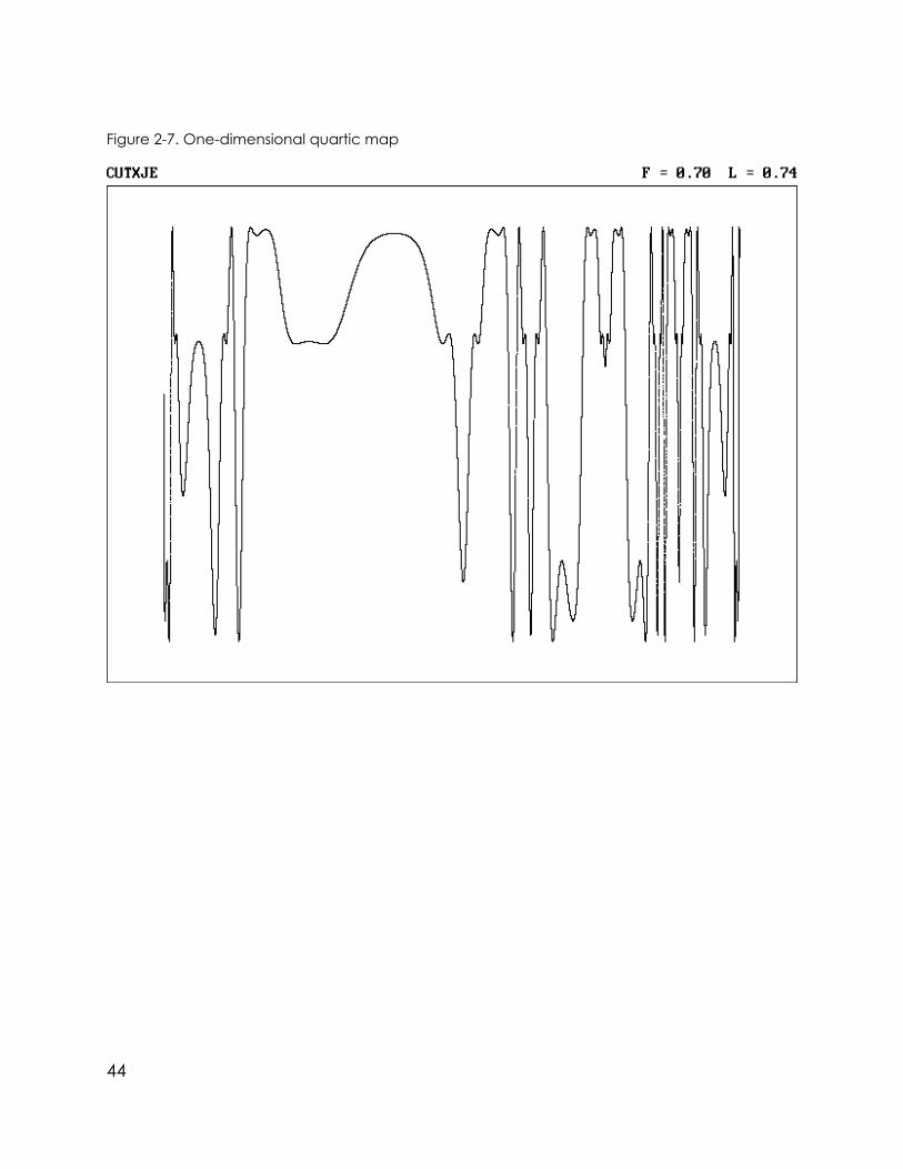
Figure 2-7. One-dimensional quartic map
44

Figure 2-8. One-dimensional quintic map
45

Figure 2-9. One-dimensional quintic map
46

Figure 2-10. One-dimensional quintic map
47
2.6 Making Music
If the preceding figures don’t qualify as art, perhaps they qualify as music.Since the quantity X behaves in a deterministic yet unpredictable way, it may bethat a sequence of musical notes determined by X will mimic the order andunpredictability that characterize music. It’s easy to test.
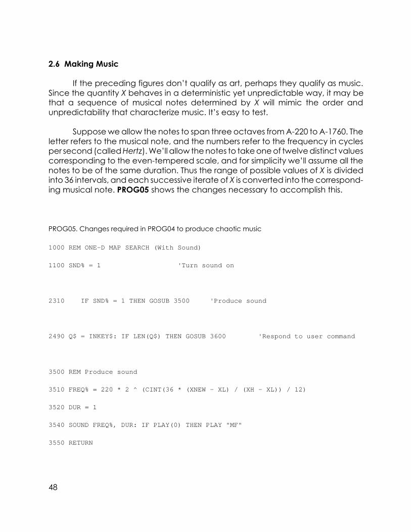
Suppose we allow the notes to span three octaves from A-220 to A-1760. Theletter refers to the musical note, and the numbers refer to the frequency in cyclesper second (called Hertz). We’ll allow the notes to take one of twelve distinct valuescorresponding to the even-tempered scale, and for simplicity we’ll assume all thenotes to be of the same duration. Thus the range of possible values of X is dividedinto 36 intervals, and each successive iterate of X is converted into the correspond-ing musical note. PROG05 shows the changes necessary to accomplish this.
PROG05. Changes required in PROG04 to produce chaotic music
1000 REM ONE-D MAP SEARCH (With Sound)
1100 SND% = 1 'Turn sound on
2310 IF SND% = 1 THEN GOSUB 3500 'Produce sound
2490 Q$ = INKEY$: IF LEN(Q$) THEN GOSUB 3600 'Respond to user command
3500 REM Produce sound
3510 FREQ% = 220 * 2 ^ (CINT(36 * (XNEW - XL) / (XH - XL)) / 12)
3520 DUR = 1
3540 SOUND FREQ%, DUR: IF PLAY(0) THEN PLAY "MF"
3550 RETURN
48

3600 REM Respond to user command
3610 T% = 0
3630 IF ASC(Q$) > 96 THEN Q$ = CHR$(ASC(Q$) - 32)
3770 IF Q$ = "S" THEN SND% = (SND% + 1) MOD 2: T% = 3
3800 RETURN
The program allows you to toggle the sound on and off by pressing the S key.Pressing any other key exits the program. You might wish to experiment with theduration DUR of the SOUND statement in line 3520. Increasing its value from 1(corresponding to approximately 0.055 seconds) makes the sounds more musical,but then the calculation takes longer.
The use of sound to help interpret data generated by a computer is atechnique that is relatively unexplored. The method is sometimes called sonification.In some cases, patterns and structure in data can be more readily discernedaudibly than visually. This technique was used to advantage in interpreting datafrom the Voyager spacecraft as it detected plasma waves near Jupiter andmicrometeorites as it crossed through the rings of Saturn. The repetitive sound of asimple limit cycle contrasts sharply with the nonrepetitive waverings of a chaotictime series.
49

Chapter 3Pieces of Planes
Whereas the last chapter discussed one-dimensional maps whose graphsare segments of lines, this chapter deals with two-dimensional maps whose graphsare pieces of planes and which thus produce much more interesting displays. Thischapter provides the minimum tools for creating attractors that genuinely qualifyas art. Armed with only the information contained here, you have such a greatvariety of available patterns that you hardly need to proceed beyond this chapter.But if you do stop here, you miss some delightful surprises.
3.1 Quadratic Maps in Two Dimensions
In the discussion so far, the maps have involved a single variable X whosevalue changes with each iteration of the equation. Such maps are said to be one-dimensional because the values of X can be thought of as lying along a line, anda line is a one-dimensional object. By plotting each value of X versus a previousvalue of X, the line can be made to wiggle with considerable complexity; but italways remains a line, and lines are of limited interest and beauty.
The situation is more interesting when you consider iterated maps that involvetwo variables, X and Y. In such a case, each iterate produces a point in a plane,where X, by convention, represents the horizontal coordinate of the point, and Yrepresents the vertical coordinate. With successive iteration, the points fill in someportion of the plane. The visually interesting cases, as usual, are the chaotic ones.
Such two-dimensional maps might arise, for example, from an ecologicalmodel only slightly more complicated than the logistic equation. A classic exampleis the predator-prey problem in which X represents the prey and Y the predator. Ina simple linear model, the solution is a fixed point (a unique number of bothpredators and prey) or a limit cycle (both the number of predators and the numberof prey oscillate, reaching their maximum values at different times, but eventuallyrepeating). When nonlinear terms are introduced into the model, the population ofeach species can behave chaotically. You can think of each point that makes upsuch an attractor as the population of predators and prey in successive years. Sincesuch complexity arises from these very simple models, it’s easy to understand whyecologists might have trouble predicting the fate of biological species!
50

Perhaps the best known chaotic two-dimensional map is the Hénon map(proposed by the French astronomer Michel Hénon in 1976), whose equations are
Xn+1 = 1 + aXn2 + bYn
Yn+1 = Xn (Equation 3A)
The quantities a and b are the control parameters, analogous to R in the logisticequation. Hénon used the values a = -1.4 and b = 0.3. The necessary nonlinearity isprovided by the X2 term in the first equation. The Hénon map is special because thenet contraction of a set of initial points covering an area of the XY plane is constantwith each iteration. The area occupied by the points is 30% of the area at theprevious iteration (from the bYn term). Other values of b can be used, but not allvalues produce chaotic solutions. Unlike the logistic map, the Hénon map isinvertable; there is a unique value for Xn and Yn corresponding to each Xn+1 andYn+1. You may have seen an alternate form of the Hénon equations in which thefactor b appears instead in the second equation and the sign preceding the X2term is negative. The result of repeated iteration of Equation 3A is shown in Figure3-1.
51

Figure 3-1. The Hénon map
The resulting graph is more than a line but less than a surface. What resemblesa single line is a pair of lines, each of which is, in turn, another pair of lines, and soforth to however close you look or whatever magnification you choose. This self-similarity is a common characteristic of a class of objects that are called fractals.
Fractals are to chaos what geometry is to algebra—the visual expression ofthe mathematical idea. Approaching an understanding of chaos through suchvisual means is appealing to those with an aversion to conventional mathematics.The Euclidean geometry we learned in high school originated with the ancientGreeks and was developed more fully by the French mathematician Descartes andothers in the 1600s. It deals with simple shapes such as lines, circles, and spheres.Euclidean geometry is now being augmented by fractal geometry, whose fatherand champion is the contemporary mathematician, Benoit Mandelbrot. Fractalsappeared in art, such as in the drawings of the Dutch artist Maurits C. Escher, before
52

they were widely appreciated by mathematicians and scientists.
Some fractals are exactly self-similar, which means that they look the sameno matter how much you magnify them. Others, such as most of the ones in thisbook, only have regions that are self-similar. There is no part of the Hénon mapwhere you can zoom in and find a miniature replica of the entire map. Other fractalsare only statistically self-similar, which means that a magnified portion of the objecthas the same amount of detail as the whole, but it is not an exact replica of it. Nearlyall strange attractors are fractals, but not all fractals arise from strange attractors.
The Hénon map produces an object with a fractal dimension that is a fractionintermediate between one and two. The fractal dimension is a useful quantity forcharacterizing strange attractors. Isolated points have dimension zero, line seg-ments have dimension one, surfaces have dimension two, and solids have dimen-sion three. Strange attractors generally have noninteger dimensions.
Some authors make a distinction between strange attractors, which havenon-interger dimension, and chaotic attractors, which exhibit sensitivity to initialconditions.
Since the Hénon map has X2 as its highest-order term, it is a quadratic map.The most general two-dimensional iterated quadratic map is
Xn+1 = a1 + a2Xn + a3Xn2 + a4XnYn + a5Yn + a6Yn
2
Yn+1 = a7 + a8Xn + a9Xn2 + a10XnYn + a11Yn + a12Yn
2 (Equation 3B)
The two equations in Equation 3B have 12 coefficients. For the Hénon map, a1 = 1,a3 = -1.4, a5 = 0.3, a8 = 1, and the other coefficients are zero. If we use the initial letterE to represent two-dimensional quadratic maps, the code for the Hénon mapaccording to Table 2-1 is EWM?MPM2WM4, where we have introduced the short-hand M2 for MM and M4 for MMMM.
Values of a in the range of -1.2 to 1.2 are sufficient to produce an enormousvariety of strange attractors. With increments of 0.1, there are 2512 or about 6 x 10¹⁶different cases, of which approximately 1.6% or about 1015 are chaotic. Viewingthem all at a rate of one per second would require over 30 million years! Stateddifferently, if each one were printed on an 81/2-by-11-inch sheet of paper, the
53

collection would cover nearly the entire land mass of Earth.
Note that not all the cases are strictly distinct. For example, if you replace Xwith Y and Y with -X in Equation 3B, you produce an attractor rotated 90 degreescounterclockwise from the original. When you do this, be sure to change Xn+1 andYn+1 as well as Xn and Yn. Thus the code EM4CMWJM3? produces a rotated versionof the Hénon map. In the same fashion, you can rotate an attractor through 180degrees by replacing X with -X and Y with -Y and through 270 degrees by replacingX with -Y and Y with X. Perhaps it’s easier just to rotate your computer monitor!
Besides rotations, there are cases that correspond to reflections. Whenviewed in a mirror, the attractors have left and right reversed, but up and downremain the same. A transformation in which X is replaced with -X accomplishes this.Thus the code for a reflected Hénon map is ECM[MJM2CM4. In addition, thereflections can be rotated. Thus there are at least eight so-called degenerate statesfor each attractor, corresponding to rotations and reflections. Such symmetries anddegeneracies play an important role in science; they often reduce the amount ofwork we have to do and provide relations between phenomena that initiallyappear different.
Additional degenerate cases correspond to scale changes. For example, ifyou replace X by mX and Y by nY with m = n, the attractor remains the same exceptit is reduced in size by a factor of m. Some of the coefficients are likely to be outsidethe allowed range, however. The Hénon map with m = n = 2 can be generated withthe code ERM1MPM2WM4. With m not equal to n, the horizontal and verticaldimensions are scaled differently, but since the computer rescales the attractor tofit the screen, the visual result is the same.
These degeneracies show that there are many ways to code a particularattractor. Although this is true, there are so many different possible combinations ofcoefficients that it is very unlikely that two degenerate cases will be found sponta-neously. Thus the examples displayed in this chapter represent but a tiny fraction ofthe possibilities, and you will be generating many other cases, almost none of whichhave been seen before.
3.2 The Butterfly Effect Revisited
Two-dimensional chaotic iterated maps also exhibit sensitivity to initial con-ditions, but the situation is more complicated than for one-dimensional maps.Imagine a collection of initial conditions filling a small circular region of the XY plane.
54

After one iteration, the points have moved to a new position in the plane, but theynow occupy an elongated region called an ellipse. The circle has contracted inone direction and expanded in the other. With each iteration, the ellipse getslonger and narrower, eventually stretching out into a long filament. The orientationof the filament also changes with each iteration, and it wraps up like a ball of taffy.
Thus two-dimensional chaotic maps have not a single Lyapunov exponentbut two—a positive one corresponding to the direction of expansion, and anegative one corresponding to the direction of contraction. The signature of chaosis that at least one of the Lyapunov exponents is positive. Furthermore, themagnitude of the negative exponent has to be greater than the positive one so thatinitial conditions scattered throughout the basin of attraction contract onto anattractor that occupies a negligible portion of the plane. The area of the ellipsecontinually decreases even as it stretches to an infinite length.
There is a proper way to calculate both of the Lyapunov exponents. For themathematically inclined, the procedure involves summing the logarithms of theeigenvalues of the Jacobian matrix of the linearized transformation with occasionalGram-Schmidt reorthonormalization. This method is slightly complicated, so we willinstead devise a simpler procedure sufficient for determining the largest Lyapunovexponent, which is all we need in order to test for chaos.
Suppose we take two arbitrary but nearby initial conditions. The first fewiterations of the map may cause the points to get closer together or farther apart,depending on the initial orientation of the two points. Eventually, the points willcome arbitrarily close in the direction of the contraction, but they will continue toseparate in the direction of the expansion. Thus if we wait long enough, the rate ofseparation will be governed only by the largest Lyapunov exponent. Fortunately,this usually takes just a few iterations.
However, because the separation grows exponentially for a chaotic system,the points quickly become too far apart for an accurate estimate of the exponent.This problem can be remedied if, after each iteration, the points are moved backto their original separation along the direction of the new separation. The Lyapunovexponent is then determined by the average of the distance they must be movedfor each iteration to maintain a constant small separation. If the two solutions areseparated by a distance dn after the nth iteration, and the separation after the nextiteration is dn+1, the Lyapunov exponent is determined from
L = ∑ log2 (dn+1 / dn) / N (Equation 3C)
where the sum is taken over all iterations from n = 0 to n = N-1. After each iteration,
55

the value of one of the iterates is changed to make dn+1 = dn. For the cases here,dn equals 10-6. This procedure also allows us to deal with maps of three and evenhigher dimensions in which there are more than two Lyapunov exponents.
3.3 Searching the Plane
We now have all the tools in hand to conduct a computer search forattractors in two dimensions. The procedure is the same as for one-dimensionalmaps, except the Lyapunov exponent calculation is done differently and the X andY variables are plotted as a point in the plane after each iteration. PROG06 showsthe changes needed to accomplish such a search.
PROG06. Changes required in PROG05 to search for two-dimensional quadratic strange attractors
1000 REM TWO-D MAP SEARCH
1060 OMAX% = 2 'Maximum order of polynomial
1070 D% = 2 'Dimension of system
1100 SND% = 0 'Turn sound off
1520 Y = .05
1550 XE = X + .000001: YE = Y
1590 XMIN = 1000000!: XMAX = -XMIN: YMIN = XMIN: YMAX = XMAX
1720 XNEW = A(1) + X * (A(2) + A(3) * X + A(4) * Y)
1730 XNEW = XNEW + Y * (A(5) + A(6) * Y)
1830 YNEW = A(7) + X * (A(8) + A(9) * X + A(10) * Y)
1930 YNEW = YNEW + Y * (A(11) + A(12) * Y)
56

2140 IF Y < YMIN THEN YMIN = Y
2150 IF Y > YMAX THEN YMAX = Y
2240 IF D% = 1 THEN XP = XS(I%): YP = XNEW ELSE XP = X: YP = Y
2250 IF N < 1000 OR XP <= XL OR XP >= XH OR YP <= YL OR YP >= YH THEN GOTO 2320
2300 PSET (XP, YP) 'Plot point on screen
2410 IF ABS(XNEW) + ABS(YNEW) > 1000000! THEN T% = 2 'Unbounded
2470 IF ABS(XNEW - X) + ABS(YNEW - Y) < .000001 THEN T% = 2
2520 Y = YNEW
2660 CODE$ = CHR$(59 + 4 * D% + O%)
2680 M% = 1: FOR I% = 1 TO D%: M% = M% * (O% + I%): NEXT I%
2910 XSAVE = XNEW: YSAVE = YNEW: X = XE: Y = YE: N = N - 1
2930 GOSUB 1700 'Reiterate equations
2940 DLX = XNEW - XSAVE: DLY = YNEW - YSAVE
2960 DL2 = DLX * DLX + DLY * DLY
2970 IF CSNG(DL2) <= 0 THEN GOTO 3070 'Don't divide by zero
2980 DF = 1000000000000# * DL2
2990 RS = 1 / SQR(DF)
3000 XE = XSAVE + RS * (XNEW - XSAVE): YE = YSAVE + RS * (YNEW - YSAVE)
3020 XNEW = XSAVE: YNEW = YSAVE
57

3030 IF DF > 0 THEN LSUM = LSUM + LOG(DF): NL = NL + 1
3040 L = .721347 * LSUM / NL
3110 IF D% = 1 THEN YMIN = XMIN: YMAX = XMAX
This program produces an incredible variety of interesting patterns, a smallselection of which is shown in Figures 3-2 through 3-17. Admire the beauty andvariety of these figures, and then make some of you own by running the program.If your computer has a printer, use the Print Screen key to print any that you findespecially appealing.
Figure 3-2. Two-dimensional quadratic map
58

Figure 3-3. Two-dimensional quadratic map
59

Figure 3-4. Two-dimensional quadratic map
60

Figure 3-5. Two-dimensional quadratic map
61

Figure 3-6. Two-dimensional quadratic map
62
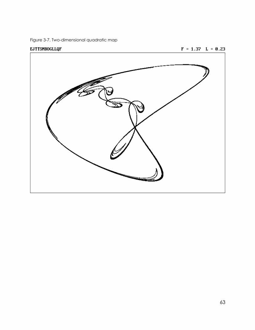
Figure 3-7. Two-dimensional quadratic map
63

Figure 3-8. Two-dimensional quadratic map
64

Figure 3-9. Two-dimensional quadratic map
65

Figure 3-10. Two-dimensional quadratic map
66
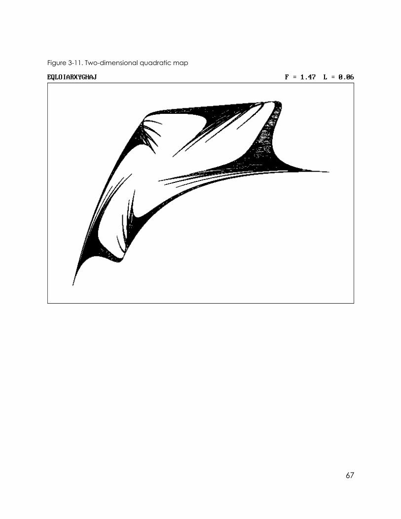
Figure 3-11. Two-dimensional quadratic map
67

Figure 3-12. Two-dimensional quadratic map
68

Figure 3-13. Two-dimensional quadratic map
69

Figure 3-14. Two-dimensional quadratic map
70

Figure 3-15. Two-dimensional quadratic map
71
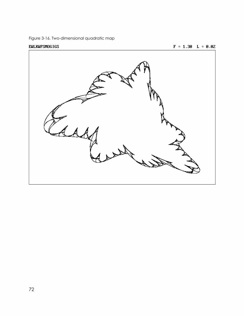
Figure 3-16. Two-dimensional quadratic map
72

Figure 3-17. Two-dimensional quadratic map
73

If you are an experienced programmer, you might consider writing a screen-saver program based on PROG06. Such a terminate-and-stay-resident (TSR) pro-gram is run once when the computer is turned on and leaves a portion of itself inmemory, constantly monitoring keyboard and mouse activity. When there is no useractivity for, say, five minutes, it blanks the screen and begins displaying a successionof unique strange attractors to prevent screen burn-in. The original screen is restoredwhenever a key is pressed or the mouse is moved. PowerBASIC version 3.0 allowsyou to do this easily by inserting the program between POPUP statements.
3.4 The Fractal Dimension
The previous figures differ considerably in how densely they fill the plane.Some are very thin, others are thick. A good contrast is provided by Figures 3-16 and3-17. Figure 3-16 resembles a piece of string that has been laid down in acomplicated shape on the page, whereas Figure 3-17 looks like a twisted piece ofpaper with many holes in it. Thus the object in Figure 3-16 has a fractal dimensionclose to 1, and the object in Figure 3-17 has a fractal dimension closer to 2.
It is possible to be more explicit and to calculate the fractal dimensionexactly. Consider two simple cases, one in which successive iterates lie uniformlyalong a straight line that goes diagonally across the page, and the other in whichsuccessive iterates gradually fill the entire plane, as if they were grains of peppersprinkled on the paper from a great height. The first case has dimension 1, and thesecond has dimension 2. How would we calculate the dimension, given the X andY coordinates of an arbitrary collection of such points?
One method is to draw a small circle somewhere on the plane that surroundsat least one of the points. We then draw a second circle with the same center butwith twice the radius. Now we count the number of points inside each circle. Let’ssay the smaller circle encloses N1 points and the larger circle encloses N2 points.Obviously N2 is greater than or equal to N1 because all the points inside the innercircle are also inside the outer circle.
If the points are widely separated, then N2 equals N1. If the points are part ofa straight line, the larger circle on average encloses twice as many points as thesmaller circle, but if the points are part of a plane, the larger circle on averageencloses four times as many points as the smaller circle, because the area of a circleis proportional to the square of its radius. Thus for these simple cases the dimensionis given by
74

F = log2 (N2 / N1) (Equation 3D)
It is hardly surprising that if you do this operation for the cases shown in the figures,the quantity F is neither 0 nor 1 nor 2 but rather a fraction.
With real data, a number of practical considerations determine the accu-racy of the result and the amount of computation required to obtain it:
1. Is a circle the best shape, or would a square, rectangle, triangle, or someother shape be better?
2. How large should the circle be?
3. Is doubling the size of the circle optimal, or would some other factor bebetter?
4. Where should the circles be placed, and how many circles are required toobtain a representative average?
5. How many points are needed to produce a reliable fractal dimension?
Let’s address each of these questions in turn.
There is nothing special about circles. A rectangle, triangle, or any other two-dimensional figure would suffice, because the area scales as the square of thelinear dimension in each case. However, a circle is convenient because it is easy totell whether a given point is in its interior by comparing the radius of the circle withthe distance of the point from its center.
The optimum size of the circle represents a compromise. Ideally, the circlesshould be invisibly small, because the dimension is defined in the limit of infiniteresolution. However, if the circles are too small, they contain too few points toproduce a statistically meaningful result, unless an unreasonably large number ofiterations is performed. We somewhat arbitrarily use circles with a radius equal toabout 2% of the diagonal of the smallest rectangle that contains the attractor.
Similarly, doubling the radius of the circle is arbitrary. Small values degradethe statistics, and large values miss too much of the fine-scale structure. We will usea value of ten, with the smaller circle about 0.6% the size of the attractor and thelarger circle about 6% the size of the attractor. Thus in Equation 3D we will uselogarithms of base 10 (log10) instead of base 2 (log2).
75

Ideally, the circles should be placed uniformly or randomly over the plane.However, if we were to do this, most of the circles would be empty, and a very longcalculation would be required to obtain an accurate estimate of the dimension.Instead, we center the circles on the data points themselves. In this way the circlestend to enclose many points. However, it represents a different type of averagebecause it weighs more heavily the portions of the attractor where the points aremost dense. Technically, what we are calculating is called the correlation dimen-sion, because it involves the number of other points that are correlated with eachpoint in the data set. The correlation dimension is never greater than the fractaldimension, but it tends not to be much smaller either.
The correlation dimension is only one of many ways to define the dimensionof an attractor. The various methods differ in how the regions of the attractor areweighed in the average. It is probably the easiest method to implement, and it givesmore reliable results than the fractal dimension when the dimension of the attractoris greater than about two. The fractal dimension is also called the capacitydimension, and it is closely related to the Hausdorff-Besicovitch dimension. Further-more, the correlation dimension is probably a more meaningful measure of thestrangeness of the attractor, because it includes information about its formation aswell as its final appearance.
The number of data points required to provide an accurate estimate of thedimension is a question still being debated in the scientific literature. Therefore, wewill use a heuristic approach and continually update the dimension estimate witheach iteration, giving you an opportunity to decide when it seems to haveconverged to a unique value. To do this, we must modify the procedure slightly.Rather than count the number of data points within a circle, which would requirethat the calculation run to conclusion with the coordinates of all the points saved,we use the equivalent method of determining the probability that two randomlychosen points are within a certain distance of one another. To do this, the distanceof each new iterate from one of its randomly chosen predecessors is calculated.Now you see why we bothered to save the last 500 iterates! We exclude the mostrecent 20 points, because the iterates are likely to be abnormally highly correlatedwith their recent predecessors. Thus, with each iteration, we have only oneadditional calculation to do in which we compare the distance of the iterate to oneof its randomly chosen predecessors and increment N1 and N2, as appropriate.PROG07 shows the changes needed to calculate and display the fractal dimen-sion.
PROG07. Changes required in PROG06 to calculate and display the fractal dimension
76

1000 REM TWO-D MAP SEARCH (With Fractal Dimension)
1020 DIM XS(499), YS(499), A(504), V(99)
1580 P% = 0: LSUM = 0: N = 0: NL = 0: N1 = 0: N2 = 0
1620 TWOD% = 2 ^ D%
2210 XS(P%) = X: YS(P%) = Y
2440 GOSUB 3900 'Calculate fractal dimension
3030 LSUM = LSUM + LOG(DF): NL = NL + 1
3060 IF N > 1000 AND N MOD 10 = 0 THEN LOCATE 1, 76: PRINT USING "##.##"; L;
3170 XL = XMIN - MX: XH = XMAX + MX: YL = YMIN - MY: YH = YMAX + 1.5 * MY
3190 YH = YH - .5 * MY
3400 LOCATE 1, 1: PRINT CODE$
3420 LOCATE 1, 63: PRINT "F =": LOCATE 1, 73: PRINT "L ="
3900 REM Calculate fractal dimension
3910 IF N < 1000 THEN GOTO 4010 'Wait for transient to settle
3920 IF N = 1000 THEN D2MAX = (XMAX - XMIN) ^ 2 + (YMAX - YMIN) ^ 2
3930 J% = (P% + 1 + INT(480 * RND)) MOD 500
3940 DX = XNEW - XS(J%): DY = YNEW - YS(J%)
77

3950 D2 = DX * DX + DY * DY
3960 IF D2 < .001 * TWOD% * D2MAX THEN N2 = N2 + 1
3970 IF D2 > .00001 * TWOD% * D2MAX THEN GOTO 4010
3980 N1 = N1 + 1
3990 F = .434294 * LOG(N2 / (N1 - .5))
4000 LOCATE 1, 66: PRINT USING "##.##"; F;
4010 RETURN
At this point you might want to examine the fractal dimension of the variousfigures in this book as well as the dimension of those you create with PROG07. Onething you will notice is that the dimension of objects that resemble lines is often lessthan 1.0. One reason is that the points that make up the line are seldom uniformlydistributed along its length. Remember that the correlation dimension is usuallysmaller than the fractal dimension. They are equal if the points are uniformlydistributed over the attractor. The correlation dimension of a line consisting of auniform distribution of points along its length would be exactly 1.0.
Also note that the dimension of most attractors varies considerably from onepart of the attractor to another. Figure 3-11 is a good example of one in which partsof the attractor resemble thin lines and other parts resemble filled-in planes. Itobviously is simplistic to characterize such an object by a single average dimension.
The dimension also depends on scale. It is properly defined in the limit whereone zooms in very tightly on the attractor to observe its finest detail. However, acalculation in this limit would take forever because an infinite number of iterationswould be required to collect enough points to reveal the detail. Figure 3-13 is anexample of an attractor that is nearly one-dimensional on a large scale but closerto two-dimensional on a fine scale. Our calculation provides what might be calleda visual dimension because it is taken on a scale close to what the eye can visuallyresolve. In any case, you should not ascribe undue significance to the calculateddimension.
Also note that we are using the word "dimension" to mean several differentthings. The maps that we are looking at are two-dimensional because they havetwo variables, X and Y. However, the attractor has a smaller dimension. We say the
78

attractor is embedded in a two-dimensional space or that the embedding dimen-sion is 2. A point or a line can be embedded in a plane, but a ball cannot.
An attractor usually fills a negligible portion of the space in which it isembedded. That’s why it’s called an attractor! Points initially distributed throughoutthe embedding space are drawn to the attractor after a number of iterations, andthe remaining space is left empty. Thus the area of an attractor embedded in a two-dimensional space is zero, and the volume of an attractor embedded in a three-dimensional space is zero, and so forth.
It is also interesting that the fractal dimension and the Lyapunov exponentsare not entirely independent. It has been conjectured that the fractal dimension isrelated to the two Lyapunov exponents by
F = 1 - L1 / L2 (Equation 3E)
where L1 is the more positive of the two exponents and is the one we denote by Lin the figures. If both Lyapunov exponents are known, Equation 3E can be used todefine a dimension of the attractor, called the Lyapunov dimension. The Lyapunovdimension is also called the Kaplan-Yorke dimension after the scientists whoproposed an extension of Equation 3E to higher dimensions.
This relation is reasonable because, if the two exponents are equal but ofopposite signs (L2 = - L1), the contraction in one direction is just offset by expansionin the other. A set of initial conditions spread out over a two-dimensional region thusmaintains its area upon successive iteration. Such a mapping is said to be area-preserving, symplectic, or Hamiltonian, after the 19th-century Irish astronomer,William Rowan Hamilton. On the other hand, if the contraction is very rapid (L2 islarge and negative), the initial conditions quickly collapse to a very elongatedellipse whose dimension is close to 1. Such a contraction is sometimes calledfilamentation.
Armed with information about the fractal dimension, you can program thecomputer to be even more selective. For example, the visually appealing attractorstend to have fractal dimensions slightly greater than 1, and thus you could rejectthose with smaller dimensions or those with dimensions close to 2. We return to thisintriguing possibility in Chapter 8.
79

3.5 Higher-Order Disorder
With one-dimensional maps, the attractors became more interesting whenwe considered terms higher than quadratic. It is straightforward to do the same withtwo-dimensional maps. For example, the most general equations for two-dimen-sional cubic maps are
Xn+1 = a1 + a2Xn + a3Xn2 + a4Xn
3 + a5Xn2Yn
+ a6XnYn + a7XnYn2 + a8Yn + a9Yn
2 + a10Yn3
Yn+1 = a11 + a12Xn + a13Xn2 + a14Xn
3 + a15Xn2Yn
+ a16XnYn + a17XnYn2 + a18Yn + a19Yn
2 + a20Yn3 (Equation 3F)
Note that there are 20 coefficients, which vastly increases the number ofpossible cases. The fourth-order case would have 30 coefficients, and the fifth-ordercase would have 42 coefficients. If you prefer an equation, a two-dimensional mapof order O has (O + 1)(O + 2) coefficients. We will code the cubic, quartic, andquintic cases with the letters F, G, and H, respectively.
The changes that must be made to the program to generate attractors in twodimensions up to fifth order are given in PROG08.
PROG08. Changes required in PROG07 to generate attractors in two dimensions up to fifth order
1000 REM TWO-D MAP SEARCH (Polynomials up to 5th Order)
1020 DIM XS(499), YS(499), A(504), V(99), XY(4), XN(4)
1060 OMAX% = 5 'Maximum order of polynomial
1720 M% = 1: XY(1) = X: XY(2) = Y
1730 FOR I% = 1 TO D%
1740 XN(I%) = A(M%)
1750 M% = M% + 1
80
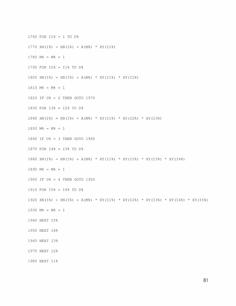
1760 FOR I1% = 1 TO D%
1770 XN(I%) = XN(I%) + A(M%) * XY(I1%)
1780 M% = M% + 1
1790 FOR I2% = I1% TO D%
1800 XN(I%) = XN(I%) + A(M%) * XY(I1%) * XY(I2%)
1810 M% = M% + 1
1820 IF O% = 2 THEN GOTO 1970
1830 FOR I3% = I2% TO D%
1840 XN(I%) = XN(I%) + A(M%) * XY(I1%) * XY(I2%) * XY(I3%)
1850 M% = M% + 1
1860 IF O% = 3 THEN GOTO 1960
1870 FOR I4% = I3% TO D%
1880 XN(I%) = XN(I%) + A(M%) * XY(I1%) * XY(I2%) * XY(I3%) * XY(I4%)
1890 M% = M% + 1
1900 IF O% = 4 THEN GOTO 1950
1910 FOR I5% = I4% TO D%
1920 XN(I%) = XN(I%) + A(M%) * XY(I1%) * XY(I2%) * XY(I3%) * XY(I4%) * XY(I5%)
1930 M% = M% + 1
1940 NEXT I5%
1950 NEXT I4%
1960 NEXT I3%
1970 NEXT I2%
1980 NEXT I1%
81

2000 NEXT I%
2010 M% = M% - 1: XNEW = XN(1): YNEW = XN(2)
PROG08 could have been written more compactly, but it is done this way tosimplify its extension to even higher dimensions. Examples of attractors produced bythis program are shown in Figures 3-18 through 3-41.
Figure 3-18. Two-dimensional cubic map
82
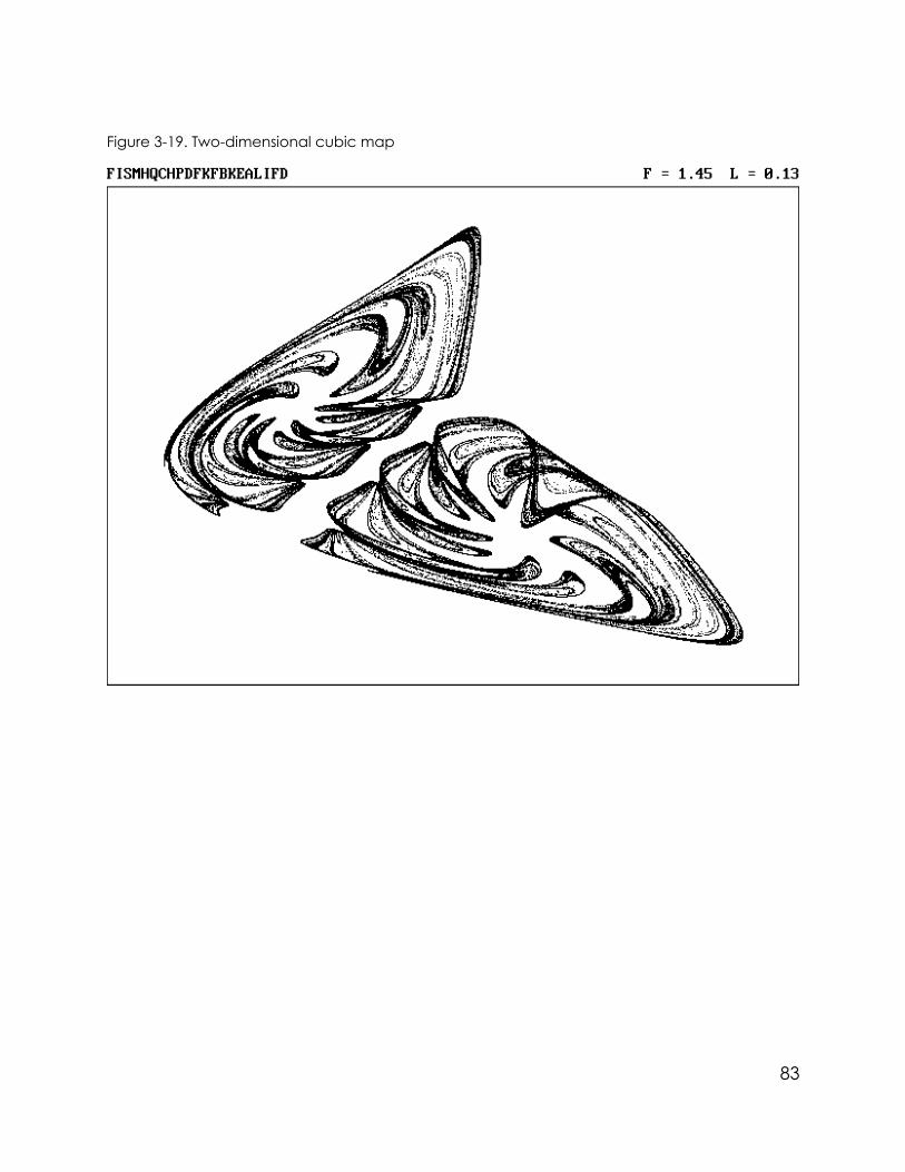
Figure 3-19. Two-dimensional cubic map
83

Figure 3-20. Two-dimensional cubic map
84

Figure 3-21. Two-dimensional cubic map
85

Figure 3-22. Two-dimensional cubic map
86
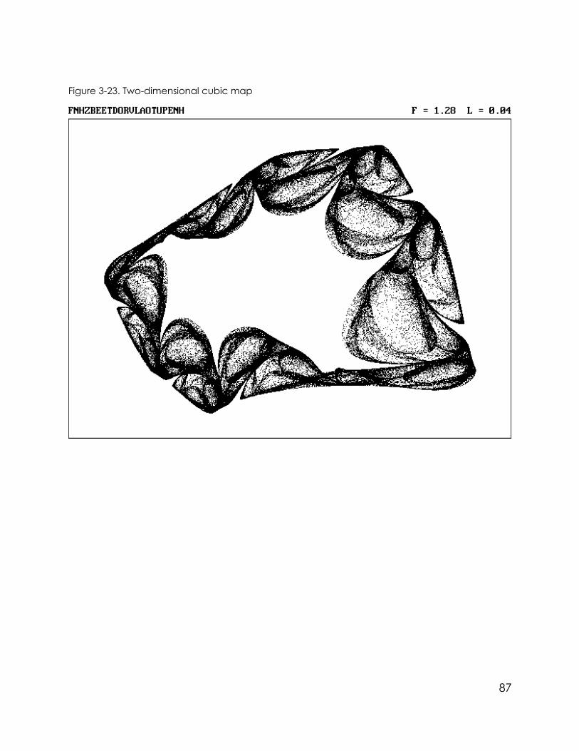
Figure 3-23. Two-dimensional cubic map
87

Figure 3-24. Two-dimensional cubic map
88

Figure 3-25. Two-dimensional cubic map
89

Figure 3-26. Two-dimensional quartic map
90

Figure 3-27. Two-dimensional quartic map
91
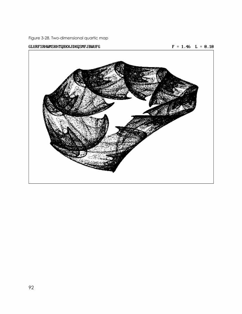
Figure 3-28. Two-dimensional quartic map
92

Figure 3-29. Two-dimensional quartic map
93

Figure 3-30. Two-dimensional quartic map
94
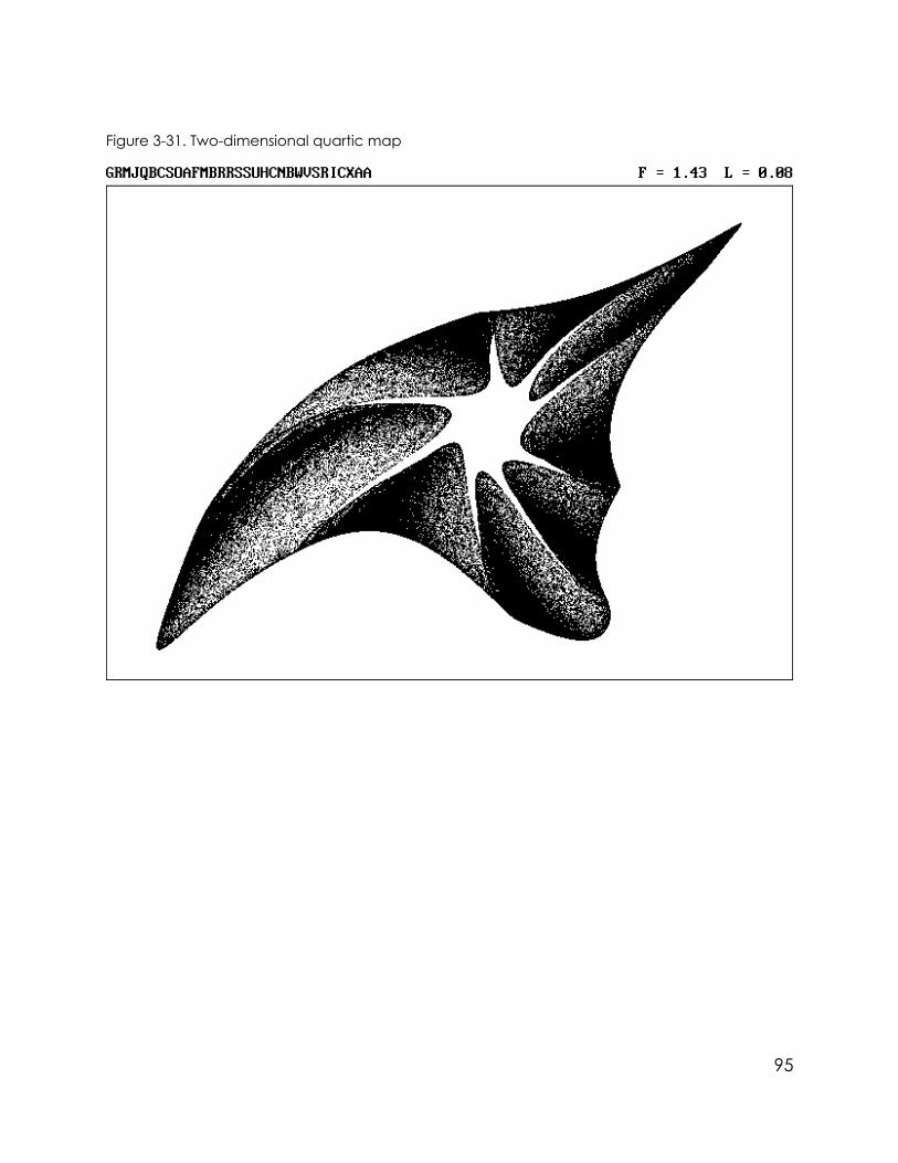
Figure 3-31. Two-dimensional quartic map
95

Figure 3-32. Two-dimensional quartic map
96

Figure 3-33. Two-dimensional quartic map
97

Figure 3-34. Two-dimensional quintic map
98

Figure 3-35. Two-dimensional quintic map
99
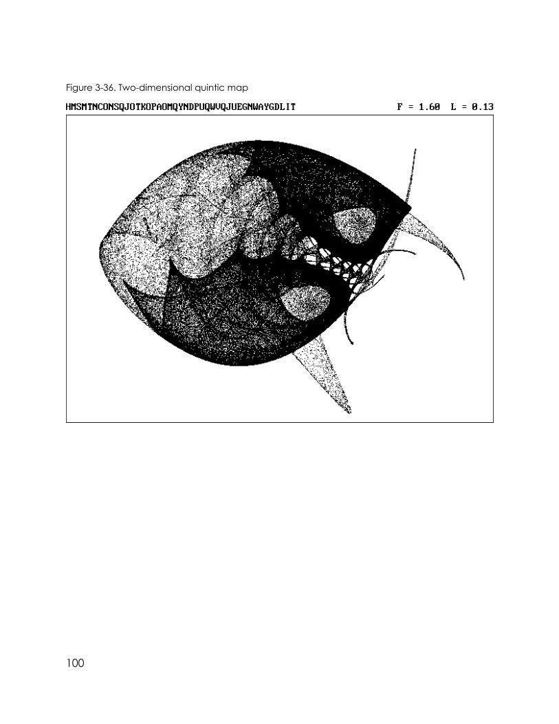
Figure 3-36. Two-dimensional quintic map
100

Figure 3-37. Two-dimensional quintic map
101

Figure 3-38. Two-dimensional quintic map
102

Figure 3-39. Two-dimensional quintic map
103
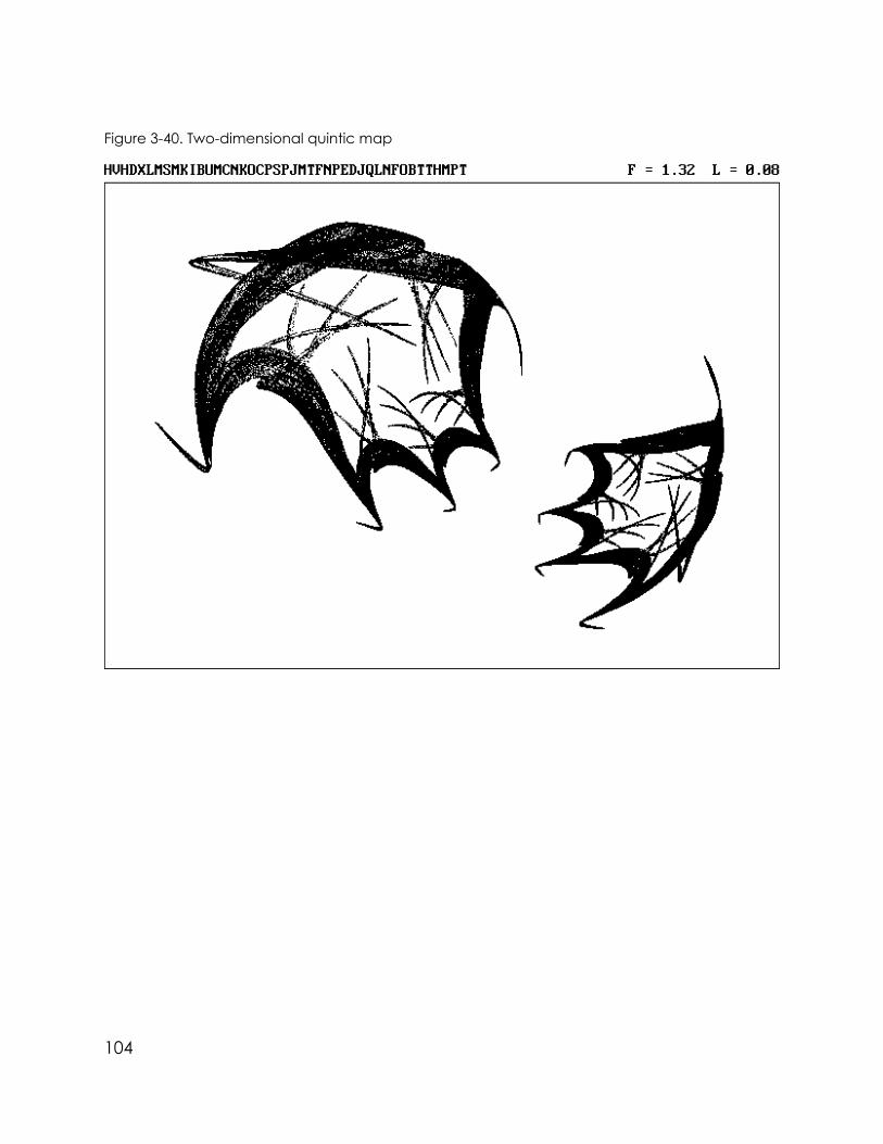
Figure 3-40. Two-dimensional quintic map
104

Figure 3-41. Two-dimensional quintic map
Perhaps this is a good point to pause and reiterate in what sense theseobjects are attractors. If you choose initial values of X and Y somewhere near theattractor, within its basin of attraction, and substitute these values into the equa-tions that describe the attractor, the new values of X and Y represent a point in theplane that is closer to the attractor. After a number of iterations, the point works itsway to the attractor, and thereafter it moves around on the attractor in somecomplicated manner, eventually visiting every part of the attractor. The nextposition can always be simply and accurately predicted from the current position,but the small, inevitable uncertainty in position continually increases so that a long-term prediction is impossible, except to say that the point is somewhere on theattractor. You can think of the attractor as the set of all possible long-term solutionsof the equations that produced it.
Besides the error in knowing perfectly the initial conditions, there are also
105

computer round-off errors at each iteration. Given the extreme sensitivity to smallerrors, you may wonder whether any computer is capable of calculating correctlysuch a chaotic process. It is true that if the same chaotic equations are iterated ontwo computers using different precision or round-off methods, the sequence ofiterates is almost certainly completely different after a few dozen iterations.However, the appearance of the attractor is probably the same. In such a case, wesay that the solution is structurally stable or robust. Furthermore, according to theshadowing lemma, an appropriate small change in initial conditions produces achaotic sequence that follows arbitrarily close to the computed one.
Since computers always round the results of calculations to a finite numberof digits (or more precisely, bits), a limited number of values is allowed. Thussuccessive iteration of a map always eventually repeats a previously obtainedvalue, whereupon the solution reproduces exactly the same sequence of states asit did before. Strictly speaking, every such solution is periodic, and true chaoscannot be observed with a computer. However, with double-precision floating-point variables, which are normally 64 bits, there are 264 or about 1019 possiblevalues. It can be shown that an average periodicity occurs after about the squareroot of this number of iterations, which is about 3 x 10⁹. Until the number of iterationsapproaches this value, there is little cause to worry. For maps higher than onedimension, this problem is even less serious because all the variables have to reacha previously existing state at the same time.
It is also interesting to realize that infinitely many periodic solutions areembedded in each attractor. These solutions are called periodic orbits. Fromwherever you start on the attractor, you eventually return to a point arbitrarily closeto the starting point. This result is called the Poincaré recurrence theorem, afterJules-Henri Poincaré, a French mathematician who a hundred years ago por-tended the modern era of chaos. Thus by making only a small change in the startingpoint, it is possible, in principle, to return exactly to the starting point, which impliesa periodic orbit with a period equal to the number of iterations required to return.Most of these orbits have very large periods, however.
Every point on the attractor is arbitrarily close to such a periodic orbit, but thechance that a randomly chosen point on the attractor lies on such an orbit isinfinitesimal. We say that the periodic orbits are dense on the attractor. These orbits,though infinite in number, constitute a Cantor set of measure zero. The periodicorbits are unstable in the sense that if you get just slightly off the orbit, you continueto get farther away with each iteration.
The strange attractors exhibited in this book are examples of orbital fractals.They should be distinguished from escape-time fractals, which show the basin of
106

attraction and typically display with color the number of iterations required forpoints outside the basin to escape beyond some predefined region. The Mandelbrotand Julia sets are perhaps the best-known escape-time fractals. Escape-timefractals require much longer computing times to develop but provide dazzlingdisplays with exotic fine-scale structures.
3.6 Strange Attractor Planets
The previous figures have obvious beauty, but they generally lack symmetry.Nature mixes symmetry with disorder, and our sense of beauty has developedaccordingly. The Earth viewed from outer space is beautiful in part because theirregular features of the clouds and continents are superimposed on a nearlyperfect sphere.
There are many ways to do the same with our attractors. Suppose, forexample, X and Y are not the horizontal and vertical positions in a plane but ratherthe longitude and latitude on the surface of the Earth. The result is an object thatmight resemble a strange planet with swirling clouds, oceans, canals, craters, andother features.
Note that mapping a plane onto a sphere is a nonlinear transformation. Youcan’t wrap a piece of paper around a globe without a large nonuniform stretching.That’s why Greenland looks larger than South America on most flat maps. When asphere is projected onto a flat computer screen or onto the page of a book, it isstretched so as to magnify the central portion of the attractor and compress theedges.
If θ is the longitude (measured from zero at the right edge) and φ is the latitude(measured from zero at the top), the X and Y coordinates of the projection of asphere onto the screen are given by
Xp = cos _ sin _
Yp = cos _ (Equation 3G)
We get θ from X by a scaling that keeps θ in the range of 0 to π radians (180degrees), because there is no need to plot points that lie on the back side of theplanet. Similarly, we get φ from Y by a scaling that keeps φ in the range of 0 (at theNorth Pole) to π radians (at the South Pole). The program modifications required toaccomplish this transformation are given in PROG09. This program allows you to
107

toggle back and forth between the two types of projection by pressing the P key.
PROG09. Changes required in PROG08 to project attractor onto a sphere
1000 REM TWO-D MAP SEARCH (Projected onto a Sphere)
1110 PJT% = 1 'Projection is spherical
2260 IF PJT% = 1 THEN GOSUB 4100 'Project onto a sphere
3200 XA = (XL + XH) / 2: YA = (YL + YH) / 2
3310 IF PJT% <> 1 THEN LINE (XL, YL)-(XH, YH), , B
3320 IF PJT% = 1 THEN CIRCLE (XA, YA), .36 * (XH - XL)
3330 TT = 3.1416 / (XMAX - XMIN): PT = 3.1416 / (YMAX - YMIN)
3750 IF Q$ = "P" THEN PJT% = (PJT% + 1) MOD 2: T% = 3: IF N > 999 THEN N = 999
4100 REM Project onto a sphere
4110 TH = TT * (XMAX - XP)
4120 PH = PT * (YMAX - YP)
4130 XP = XA + .36 * (XH - XL) * COS(TH) * SIN(PH)
4140 YP = YA + .5 * (YH - YL) * COS(PH)
4150 RETURN
Figures 3-42 through 3-57 show some examples of two-dimensional attractors
108

projected onto a sphere. Note that the features on the attractors tend to convergeat the poles at the tops and bottoms of the figures. This convergence could besuppressed by using an area-preserving transformation that stretches the Y valuesnear the poles by the same factor that the X values are compressed. The simplestway to produce this effect is to delete line 4140.
Figure 3-42. Two-dimensional quadratic map projected onto a sphere
109

Figure 3-43. Two-dimensional quadratic map projected onto a sphere
110

Figure 3-44. Two-dimensional quadratic map projected onto a sphere
111

Figure 3-45. Two-dimensional quadratic map projected onto a sphere
112

Figure 3-46. Two-dimensional cubic map projected onto a sphere
113

Figure 3-47. Two-dimensional cubic map projected onto a sphere
114
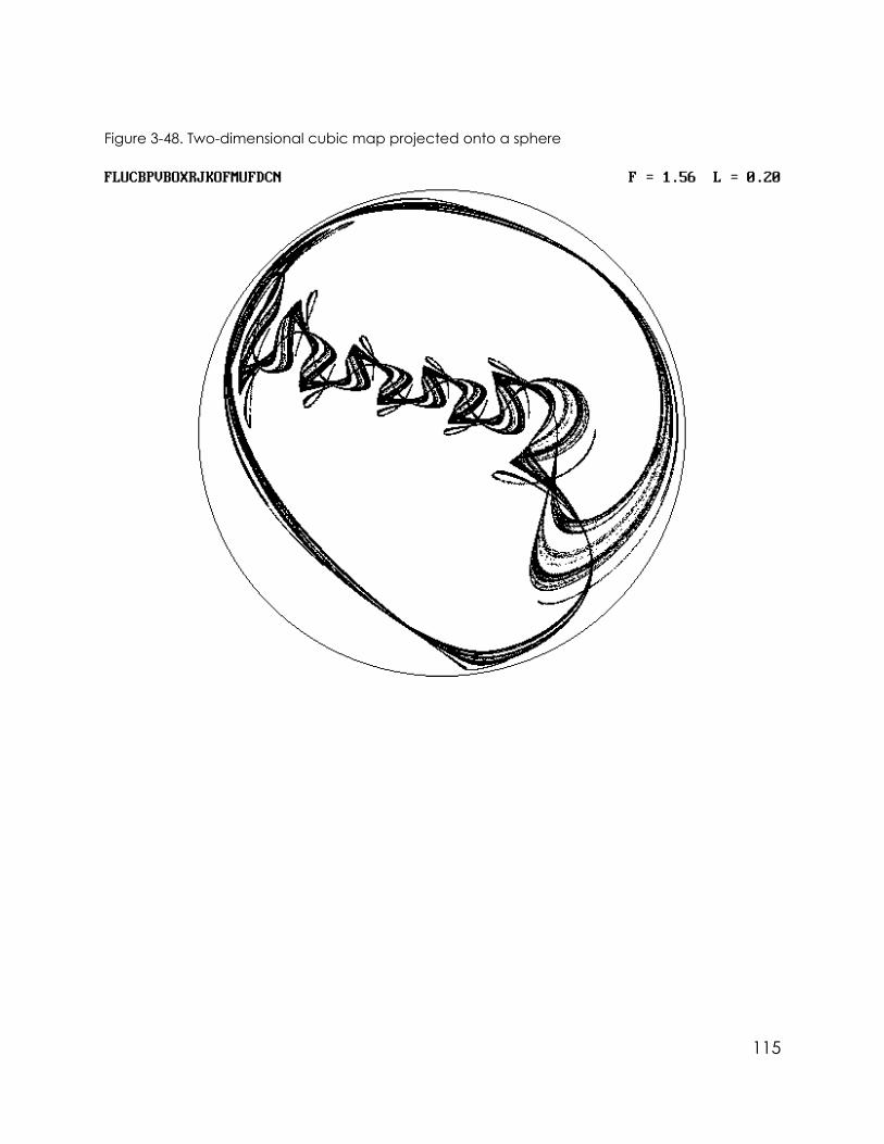
Figure 3-48. Two-dimensional cubic map projected onto a sphere
115

Figure 3-49. Two-dimensional cubic map projected onto a sphere
116

Figure 3-50. Two-dimensional quartic map projected onto a sphere
117

Figure 3-51. Two-dimensional quartic map projected onto a sphere
118

Figure 3-52. Two-dimensional quartic map projected onto a sphere
119
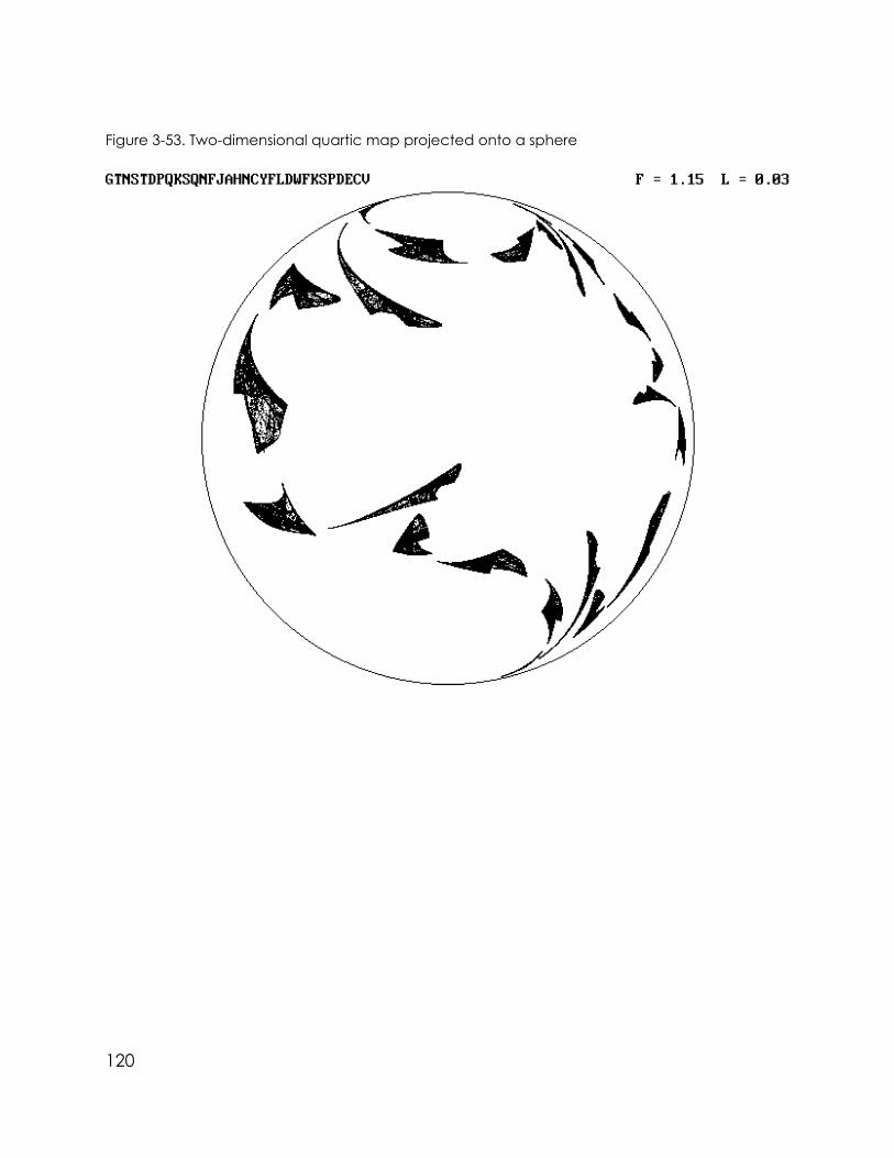
Figure 3-53. Two-dimensional quartic map projected onto a sphere
120

Figure 3-54. Two-dimensional quintic map projected onto a sphere
121

Figure 3-55. Two-dimensional quintic map projected onto a sphere
122

Figure 3-56. Two-dimensional quintic map projected onto a sphere
123
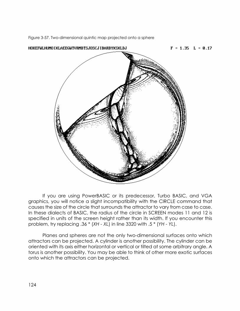
Figure 3-57. Two-dimensional quintic map projected onto a sphere
If you are using PowerBASIC or its predecessor, Turbo BASIC, and VGAgraphics, you will notice a slight incompatibility with the CIRCLE command thatcauses the size of the circle that surrounds the attractor to vary from case to case.In these dialects of BASIC, the radius of the circle in SCREEN modes 11 and 12 isspecified in units of the screen height rather than its width. If you encounter thisproblem, try replacing .36 * (XH - XL) in line 3320 with .5 * (YH - YL).
Planes and spheres are not the only two-dimensional surfaces onto whichattractors can be projected. A cylinder is another possibility. The cylinder can beoriented with its axis either horizontal or vertical or tilted at some arbitrary angle. Atorus is another possibility. You may be able to think of other more exotic surfacesonto which the attractors can be projected.
124

3.7 Designer Plaids
It is interesting that all the one-dimensional maps described in the previouschapter are included in the two-dimensional cases. One needs only to set thecoefficients of the Y equation to zero. For example, a two-dimensional mapequivalent to the logistic equation is given by the code EMu%M9. However,because Y doesn’t change with successive iterations, a graph of Y versus X is simplya straight, horizontal line.
To display the logistic parabola, we need to replace X with the next iterateof X and Y with the second next iterate of X. Two successive iterations of a quadraticmap requires a fourth-order equation. A code that accomplishes this isGMu%M13NHUIM10.
There are other examples of two-dimensional maps that are really one-dimensional maps in disguise. Suppose Xn+1 depends only on Yn and Yn+1depends only on Xn. Then Xn+2 depends only on Xn, and we have a one-dimensional map for X in which Y is merely an intermediate value of X. The mostgeneral fifth-order polynomial example of such a case is
Xn+1 = a1 + a17Yn + a18Yn2 + a19Yn
3 + a20Yn4 + a21Yn
5
Yn+1 = a22 + a23Xn + a24Xn2 + a25Xn
3 + a26Xn4 + a27Xn
5 (Equation 3H)
This case can be achieved by setting the remaining 30 coefficients to zero inPROG09 by adding the following line after line 2730:
2735 IF (I% > 1 AND I% < M% / 2 - O%) OR I% > M% / 2 + O% + 1 THEN MID$(CODE$,I% + 1, 1) = "M"
The result is to produce a 25th-order, one-dimensional polynomial map displayedin two dimensions.
Figures 3-58 through 3-61 show sample attractors obtained in this way. Noticethat they fill in rectangular regions resembling a plaid tartan, in sharp contrast to allthe previous cases. These attractors are especially appropriate for projecting ontospheres because the features line up east-west along parallels and north-southalong meridians. Figures 3-62 and 3-63 show some examples of plaid planetaryattractors.
125

Figure 3-58. Two-dimensional quadratic plaid map
126

Figure 3-59. Two-dimensional cubic plaid map
127
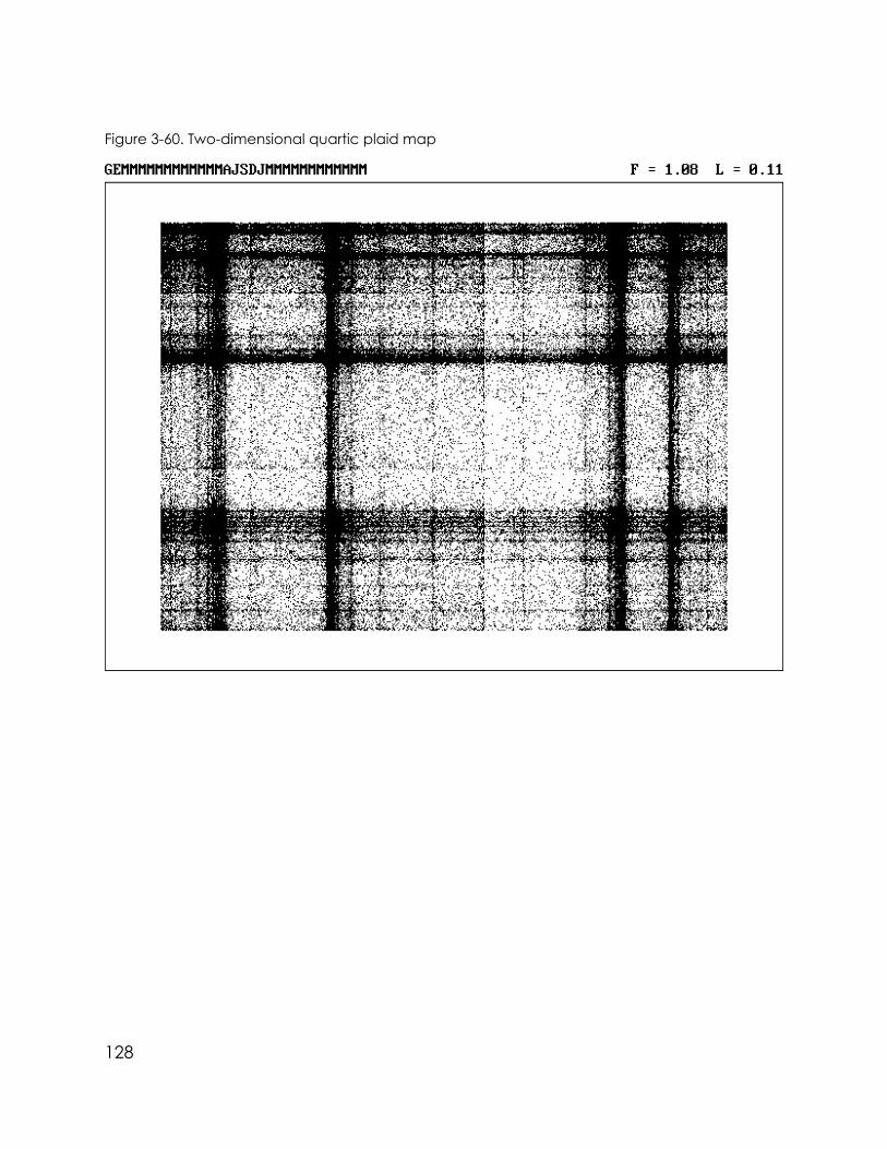
Figure 3-60. Two-dimensional quartic plaid map
128

Figure 3-61. Two-dimensional quintic plaid map
129

Figure 3-62. Two-dimensional quadratic plaid map on a sphere
130

Figure 3-63. Two-dimensional quintic plaid map on a sphere
You might want to try adding colors to emulate a decorative cloth pattern.One way to do this is to color the pixels according to the number of times they arevisited by the orbit. This is easily done by changing line 2300 in the program to
2300 PSET (XP, YP), (POINT (XP, YP) + 1) MOD 16
which causes the color of the existing point at (XP, YP) to be tested and then plottedwith the next color in the palette of 16 colors. In Chapter 4, we discuss other waysto produce colorful attractors.
131

3.8 Strange Attractors that Don’t
From the foregoing discussion, you might conclude that all chaotic equa-tions produce strange attractors. Such is not the case. Under certain conditions, thesuccessive iterates of an equation wanders chaotically throughout a region of theplane. There is no basin of attraction, and initial conditions near but outside thechaotic region are not drawn to the region but rather lie on closed curves. Althoughthe chaotic region is not a strange attractor, it may have considerable beauty.
For a chaotic solution not to attract, the area occupied by a cluster of nearbyinitial conditions must remain the same with successive iterations. The clustergenerally contracts in one direction and expands in the other, but the contractionand expansion just cancel, producing a long, thin filament of constant area. Acharacteristic of such a case is that the two Lyapunov exponents are equal inmagnitude but of opposite signs. Such a system is area-preserving. An importantclass of area-preserving systems are Hamiltonian systems with their correspondingsymplectic maps.
You might think that Hamiltonian systems are relatively rare in nature, be-cause they require a special condition. However, there are many importantexamples of Hamiltonian chaos. They arise because there are quantities in naturesuch as energy and angular momentum that, in the absence of friction, remainaccurately constant no matter how complicated the behavior of the system. Wesay these quantities are conserved or that they are constants of the motion. Themotion of a planet orbiting a binary-star system or the motion of an electron nearthe null in a magnetic field exhibits Hamiltonian chaos. A more familiar example isthe filamentation of milk when it is stirred into coffee, in which case the volume ofthe milk is conserved because liquids are nearly incompressible.
With equations such as those we have been using with randomly chosencoefficients, the chance of inadvertently finding an area-preserving solution isessentially zero. However, by placing appropriate conditions on the coefficients,we can guarantee such solutions. The following is an example of an area-preserv-ing, two-dimensional polynomial map:
Xn+1 = a1 + a2Xn + a3Xn2 + a4Xn
3 + a5Xn4 + a6Xn
5 ± Yn
Yn+1 = a22 ± Xn (Equation 3I)
This map is fifth order to provide seven arbitrary coefficients that ensure alarge number of solutions. The coefficient labels are consistent with the general two-dimensional fifth-order map, in which 33 of the coefficients have been set to zero.
132

The two terms preceded with ± have coefficients (a17 and a23) of either +1 or -1,and this feature guarantees an area-preserving solution. If the signs are the same(both plus or both minus), chaotic solutions are not found. Hamiltonian chaos canoccur when the signs are opposite. The negative product of these two coefficientsis the Jacobian of the map (J = -a17a23). The Jacobian is a measure of the netcontraction, and it must equal 1.0 for a Hamiltonian system.
Hamiltonian cases can be produced by adding the following lines to PROG09after line 2730:
2735 IF I% > O% + 1 AND I% <> M% / 2 + 1 THEN MID$(CODE$, I% + 1, 1)= "M"
2736 MID$(CODE$, M% / 2 - O% + 2, 1) = "W": MID$(CODE$, M% / 2 + 3, 1)= "C"
Sample chaotic symplectic maps are shown in Figures 3-64 through 3-71.Most of the cases resemble chains of islands in which each island contains a fixedpoint surrounded by closed contours that are not shown. These cases wereproduced using initial values of X = Y = 0.05. Other initial conditions would producecompletely different pictures because there is no attractor.
133

Figure 3-64. Two-dimensional quintic symplectic map
134

Figure 3-65. Two-dimensional quintic symplectic map
135

Figure 3-66. Two-dimensional quintic symplectic map
136
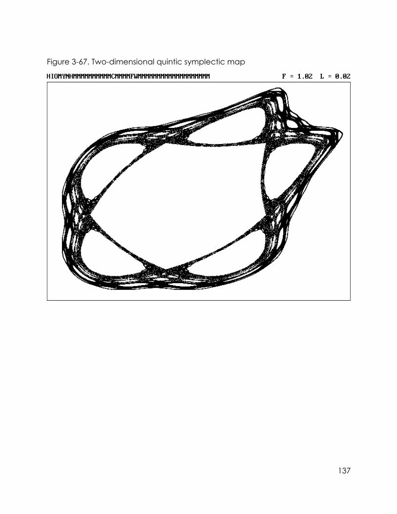
Figure 3-67. Two-dimensional quintic symplectic map
137

Figure 3-68. Two-dimensional quintic symplectic map
138

Figure 3-69. Two-dimensional quintic symplectic map
139

Figure 3-70. Two-dimensional quintic symplectic map
140

Figure 3-71. Two-dimensional quintic symplectic map
These cases have a different look from non-symplectic strange attractors.The difference is even more pronounced if you watch while they develop on thecomputer screen. Whereas the regions of a strange attractor tend to be visiteduniformly and apparently randomly, the symplectic maps develop much moreslowly. The points often wander over a small region for tens of thousands ofiterations, and then they suddenly begin to fill in a new distinct region that has neverbeen visited before. Consequently, many more iterations are required to determinethe stability and chaotic nature of the solution. You need to be patient while thecomputer calculates.
The different time behavior of these cases raises an important issue. Whenyou view any of the figures in this book, you are seeing a static object. However, itwas produced by a dynamic process. Information about the sequence in which thepoints accumulated has been lost. This additional information is recovered when
141

you watch the attractors develop on your computer screen. Most of the attractorsfill in uniformly. Their contrast gets progressively greater, much like a photographicprint being developed.
However, the symplectic maps develop more slowly and in stages. If yourcomputer has a color monitor, you might try exhibiting this sequence by plotting thepoints in color and changing the color every few thousand iterations. Someexamples using this technique are shown in Section 7.5. If you try this for the non-symplectic attractors, the colors overlap and merge into a uniform gray, or you justsee the most recent color. For the symplectic maps, beautiful color patterns can beproduced. Otherwise, continue on to the next chapter, where various colortechniques are discussed.
3.9 A New Dimension in Sound
With one-dimensional maps, we tried to make music by letting successiveiterates control the pitch of the musical notes, all of which were of the sameduration. The same procedure can be used with two-dimensional maps. However,we have a second variable at our disposal, so let’s use it to control the duration ofeach note. With actual music, it turns out that there are many more notes of shortduration than of long duration. There are roughly twice as many half notes as wholenotes, and twice as many quarter notes as half notes, and so forth. This remarkableresult seems to hold for all types of music from different composers and cultures. Itis evidence of hidden determinism in music.
The program modification PROG10 uses the X value to control the pitch andthe Y value to control the duration of the notes. For convenience, we assume thatthe longest note is a whole note and the shortest note is a sixteenth note. Dottednotes and rests are not allowed.
PROG10 also adds to the program a menu screen that reminds you of the Scommand, which toggles the sound on and off, and the P command, whichtoggles the projection between planar and spherical. We also introduce an Acommand to initiate the search for attractors, a D command to toggle betweenone-dimensional and two-dimensional maps, an I command to let you input thecode of an attractor that you know, and an X command to exit the program.Pressing any other key displays the menu screen.
142

PROG10. Changes required in PROG09 to produce chaotic music and provide a menu screen
1000 REM TWO-D MAP SEARCH (With Music and Menu Screen)
1100 SND% = 1 'Turn sound on
1110 PJT% = 0 'Projection is planar
1170 GOSUB 4200 'Display menu screen
1180 IF Q$ = "X" THEN GOTO 1250 'Exit immediately on command
2450 IF QM% > 0 THEN GOTO 2490 'Skip tests when not in search mode
2640 IF QM% > 0 THEN GOTO 2730 'Not in search mode
2650 O% = 2 + INT((OMAX% - 1) * RND)
2660 CODE$ = CHR$(59 + 4 * D% + O%)
2680 GOSUB 4700 'Get value of M%
3530 IF D% > 1 THEN DUR = 2 ^ INT(.5 * (YH - YL) / (YNEW - 9 * YL / 8 + YH / 8))
3610 IF ASC(Q$) > 96 THEN Q$ = CHR$(ASC(Q$) - 32) 'Convert to upper case
3630 IF Q$ = "" OR INSTR("ADIPSX", Q$) = 0 THEN GOSUB 4200
3640 IF Q$ = "A" THEN T% = 1: QM% = 0
3680 IF Q$ = "D" THEN D% = 1 + (D% MOD 2): T% = 1
3730 IF Q$ = "I" THEN IF T% <> 1 THEN SCREEN 0: WIDTH 80: COLOR 15, 1: CLS : LINEINPUT "Code? "; CODE$: IF CODE$ = "" THEN Q$ = " ": CLS : ELSE T% = 1: QM% = 1:GOSUB 4700
3790 IF Q$ = "X" THEN T% = 0
143

4200 REM Display menu screen
4210 SCREEN 0: WIDTH 80: COLOR 15, 1: CLS
4220 WHILE Q$ = "" OR INSTR("AIX", Q$) = 0
4230 LOCATE 1, 27: PRINT "STRANGE ATTRACTOR PROGRAM"
4260 PRINT : PRINT
4270 PRINT TAB(27); "A: Search for attractors"
4300 PRINT TAB(27); "D: System is"; STR$(D%); "-D polynomial map"
4370 PRINT TAB(27); "I: Input code from keyboard"
4400 PRINT TAB(27); "P: Projection is ";
4410 IF PJT% = 0 THEN PRINT "planar "
4420 IF PJT% = 1 THEN PRINT "spherical"
4540 PRINT TAB(27); "S: Sound is ";
4550 IF SND% = 0 THEN PRINT "off"
4560 IF SND% = 1 THEN PRINT "on "
4600 PRINT TAB(27); "X: Exit program"
4610 Q$ = INKEY$
4620 IF Q$ <> "" THEN GOSUB 3600 'Respond to user command
4630 WEND
4640 RETURN
4700 REM Get dimension and order
4710 D% = 1 + INT((ASC(LEFT$(CODE$, 1)) - 65) / 4)
144

4740 O% = 2 + (ASC(LEFT$(CODE$, 1)) - 65) MOD 4
4750 M% = 1: FOR I% = 1 TO D%: M% = M% * (O% + I%): NEXT I%
4770 IF LEN(CODE$) = M% + 1 OR QM% <> 1 THEN GOTO 4810
4780 BEEP 'Illegal code warning
4790 WHILE LEN(CODE$) < M% + 1: CODE$ = CODE$ + "M": WEND
4800 IF LEN(CODE$) > M% + 1 THEN CODE$ = LEFT$(CODE$, M% + 1)
4810 RETURN
As you listen to the music produced by the various attractors, you maydiscover relations between the quality of the music and the appearance of theattractor. The cases that seem most musical tend to have certain visual character-istics, which are left for you to discover. Do attractors that appeal to the eye alsoappeal to the ear?
After you have generated some music of your own, you may want to try someof the cases in Table 3-1 using the I command to input them to the program. Thesecases have been selected for their musical quality and are limited to quadraticmaps to simplify typing their codes. An interesting study would be to accumulateyour own longer list of musical attractors and to see if they preferentially havecertain fractal dimensions and Lyapunov exponents. If so, then it should be possibleto program the computer to be a music critic as well as an art critic.
145

Table 3-1. List of some musical attractors and their characteristics
Code F L Code F L
EDFLQJGDGMSJV 1.17 0.35 EPLKQNGALTVDD 1.03 0.20
EGITIKLJNSKAT 1.19 0.04 EQVHVRXREMJED 1.50 0.19
EHXJCQMYLONDK 0.95 0.12 ERKKCUNHERKAV 1.51 0.47
EJETCOHRSIQFN 1.56 0.25 ESHKBEWJFUOPJ 1.43 0.39
EKLVEVAOSGYJX 1.12 0.20 ETFJJNMKESAFX 0.97 0.30
ELLNJNEAMPLDX 1.11 0.64 EUFLXKIETROOO 0.90 0.40
ENIDATWFTPOSL 1.62 0.26 EVHEQLLDMMBFP 1.47 0.49
EOKYEVMDXXJUP 0.84 0.22 EXJNXAIFANNEN 1.60 0.17
After listening to the enormous variety of musical sequences that can begenerated by this technique, you might wonder whether your favorite musicalcomposition could be compressed into a short code and generated using iteratedmaps. After all, even the simple cases in Table 3-1 are chosen from among about6 x 1016 different codes, and each code corresponds to a different piece of music.
However, a typical musical piece might have hundreds or thousands ofnotes, each of which can represent dozens of pitches and many durations. Thus wecan be fairly confident using the principles of information theory that such extremecompression is unlikely, unless music has considerably more structure than isapparent. However, if you only want to generate a short tune with a few notes,there might well be a way to do so using this technique. If you are mathematicallyinclined, take it as a challenge to find a way to do this.
The generation of computer music using chaotic iterated maps is a promisingtechnique still in its infancy. You may want to incorporate more sophisticatedmusical rules into the program to generate music that is much more pleasing thanwhat results from this simple procedure. Furthermore, an interesting project wouldbe to turn the process around and see if music written by humans resembles astrange attractor, and if so, to measure its fractal dimension and Lyapunovexponent. Perhaps music of different types or by different composers would havedifferent values of these quantities.
146

Chapter 4Attractors of Depth
A two-dimensional world is a mere shadow of reality. The techniques de-scribed in the previous chapters are easily extended to produce attractors embed-ded in the three-dimensional space in which we live. The challenge is in finding waysto exhibit and visualize such three-dimensional objects within the limitations of thecomputer screen and printed page. This chapter emphasizes new visualizationtechniques and provides many new examples of strange attractors that havedepth as well as width and height.
4.1 Projections
The procedure for seeking attractors in three dimensions (which we mightwhimsically call strange attractors of the third kind) is just like the two-dimensionalcase, except that we introduce a third variable Z to accompany X and Y. You canthink of Z as representing the position in a direction out of the screen or page onwhich the attractor is displayed. We assume the direction of positive Z is in front ofthe page and the direction of negative Z is behind the page, as is customary for aconventional right-handed coordinate system. The term right-handed comes fromthe convention that if you point the fingers of your right hand in the direction of theX-axis and curl them so that they point along the Y-axis, your thumb points in the Zdirection. This choice is purely arbitrary but widely accepted.
The simplest system of equations that produces strange attractors embed-ded in a three-dimensional space is a set of coupled quadratic equations, the mostgeneral form of which is given by
Xn+1 = a1 + a2Xn + a3Xn2 + a4XnYn + a5XnZn + a6Yn
+ a7Yn2 + a8YnZn + a9Zn + a10Zn
2
Yn+1 = a11 + a12Xn + a13Xn2 + a14XnYn + a15XnZn + a16Yn
+ a17Yn2 + a18YnZn + a19Zn + a20Zn
2
Zn+1 = a21 + a22Xn + a23Xn2 + a24XnYn + a25XnZn + a26Yn
147

+ a27Yn2 + a28YnZn + a29Zn + a30Zn
2 (Equation 4A)
These equations have 30 coefficients, which allow an enormous variety ofattractors. The extension to equations with orders higher than two is straightforward.Three-dimensional cubic equations have 60 coefficients, quartic equations have105 coefficients, and quintic equations have 168 coefficients. The number ofcoefficients for order O is given by (O + 1)(O + 2)(O + 3) / 2. We will code the second-order through fifth-order systems in three dimensions with the initial letters I, J, K, andL, respectively.
Note that 168 coefficients allows 25168 or about 10234 combinations. This isa truly astronomical number. Even if only a small fraction of them correspond todistinct strange attractors, their number enormously exceeds the number of elec-trons, protons, and neutrons in the entire universe—a mere 1079. Thus the numberof fifth-order three-dimensional strange attractors is essentially infinite. You canhave a large collection of your own, none of which are likely to be reproduced byanyone else unless you give them the code you used to produce them. The codeis like a combination lock with 168 settings that all must be entered correctly and inthe proper order.
Now we must confront the issue of how best to display an object composedof points in a three-dimensional space. Such problems are in the domain of a newspecialty called visualization, which we may define as the use of computer imageryto gain insight into complex phenomena. The need for improved visualizationtechniques has emerged from the rapidly growing use of computers as the primarytool for scientific calculation and modeling. As computers become more powerful,it is increasingly important to devise methods of dealing with large quantities ofdata. The eye and brain are very efficient at discerning visual patterns, and thesepatterns permit an intuitive understanding of complicated processes in a way thatequations often cannot. Scientists have recently developed impressive visualiza-tion techniques, simple versions of which are presented here.
The simplest method is to ignore one of the coordinates and to plot the pointsin the remaining two dimensions. This method is equivalent to looking at the shadowcast by an object when illuminated from directly above by a point-source of lighta large distance away. If the light source is on the Z-axis, we say the attractor isprojected onto the XY plane. The screen used in conjunction with a slide projectoris such a plane. Of course, considerable information about the attractor is lost insuch a projection, but the method is a convenient starting point, and it is simple toprogram.
PROG11 provides the changes that must be made in PROG10 to extend the
148

attractor search to three dimensions with order up to five. Since the search slowsdown considerably in three dimensions with such a large number of coefficients,especially if you don’t have a compiled version of BASIC and a fast computer, theprogram saves, for each case found, the code, fractal dimension, and Lyapunovexponent in a disk file with the name SA.DIC (Strange Attractor DICtionary). Thisfeature allows you to run the program unattended and to collect the attractors itfinds. We will later modify the program to let you examine the cases that you collect.
PROG11. Changes required in PROG10 to search for strange attractors in three dimensions
1000 REM THREE-D MAP SEARCH
1020 DIM XS(499), YS(499), ZS(499), A(504), V(99), XY(4), XN(4)
1070 D% = 3 'Dimension of system
1100 SND% = 0 'Turn sound off
1530 Z = .05
1550 XE = X + .000001: YE = Y: ZE = Z
1600 ZMIN = XMIN: ZMAX = XMAX
1720 M% = 1: XY(1) = X: XY(2) = Y: XY(3) = Z
2010 M% = M% - 1: XNEW = XN(1): YNEW = XN(2): ZNEW = XN(3)
2160 IF Z < ZMIN THEN ZMIN = Z
2170 IF Z > ZMAX THEN ZMAX = Z
2210 XS(P%) = X: YS(P%) = Y: ZS(P%) = Z
2410 IF ABS(XNEW) + ABS(YNEW) + ABS(ZNEW) > 1000000! THEN T% = 2
149

2460 IF N >= NMAX THEN T% = 2: GOSUB 4900 'Strange attractor found
2470 IF ABS(XNEW - X) + ABS(YNEW - Y) + ABS(ZNEW - Z) < .000001 THEN T% = 2
2530 Z = ZNEW
2910 XSAVE = XNEW: YSAVE = YNEW: ZSAVE = ZNEW
2920 X = XE: Y = YE: Z = ZE: N = N - 1
2950 DLZ = ZNEW - ZSAVE
2960 DL2 = DLX * DLX + DLY * DLY + DLZ * DLZ
3010 ZE = ZSAVE + RS * (ZNEW - ZSAVE)
3020 XNEW = XSAVE: YNEW = YSAVE: ZNEW = ZSAVE
3140 IF ZMAX - ZMIN < .000001 THEN ZMIN = ZMIN - .0000005: ZMAX = ZMAX + .0000005
3400 LOCATE 1, 1: IF LEN(CODE$) < 62 THEN PRINT CODE$
3410 IF LEN(CODE$) >= 62 THEN PRINT LEFT$(CODE$, 57) + "..."
3680 IF Q$ = "D" THEN D% = 1 + (D% MOD 3): T% = 1
3920 IF N = 1000 THEN D2MAX = (XMAX - XMIN) ̂ 2 + (YMAX - YMIN) ̂ 2 + (ZMAX - ZMIN)^ 2
3940 DX = XNEW - XS(J%): DY = YNEW - YS(J%): DZ = ZNEW - ZS(J%)
3950 D2 = DX * DX + DY * DY + DZ * DZ
4760 IF D% = 3 THEN M% = M% / 2
150
4900 REM Save attractor to disk file SA.DIC
4910 OPEN "SA.DIC" FOR APPEND AS #1
4920 PRINT #1, CODE$; : PRINT #1, USING "##.##"; F; L
4930 CLOSE #1
4940 RETURN
Some examples of the attractors produced by PROG11 are shown in Figures4-1 through 4-16. Note that the fractal dimension shown for each case is thedimension of the actual attractor and not the dimension of its projection. Thus thefractal dimension can be as large as 3 even though the projection has dimensionof at most 2. The projection of a point (zero dimensions) onto a surface is a point,the projection of a line (one dimension) is a line, the projection of a surface (twodimensions) is a surface, but the projection of a solid (three dimensions) onto asurface is only a surface (two dimensions).
151

Figure 4-1. Projection of three-dimensional quadratic map
152

Figure 4-2. Projection of three-dimensional quadratic map
153

Figure 4-3. Projection of three-dimensional quadratic map
154

Figure 4-4. Projection of three-dimensional quadratic map
155

Figure 4-5. Projection of three-dimensional quadratic map
156

Figure 4-6. Projection of three-dimensional quadratic map
157

Figure 4-7. Projection of three-dimensional quadratic map
158

Figure 4-8. Projection of three-dimensional quadratic map
159

Figure 4-9. Projection of three-dimensional cubic map
160
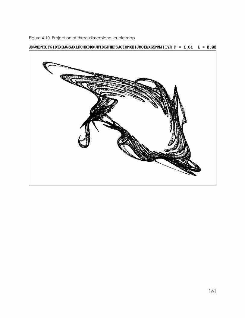
Figure 4-10. Projection of three-dimensional cubic map
161

Figure 4-11. Projection of three-dimensional cubic map
162

Figure 4-12. Projection of three-dimensional quartic map
163

Figure 4-13. Projection of three-dimensional quartic map
164
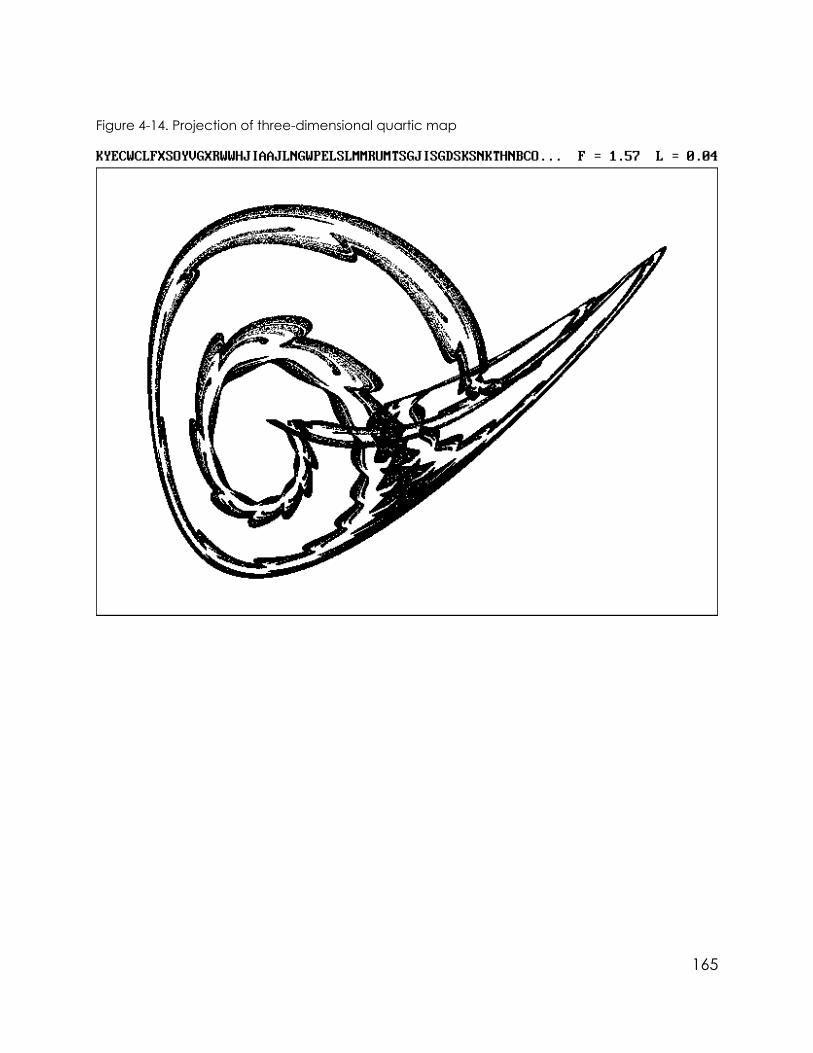
Figure 4-14. Projection of three-dimensional quartic map
165

Figure 4-15. Projection of three-dimensional quintic map
166

Figure 4-16. Projection of three-dimensional quintic map
On the whole, attractors in three dimensions projected onto a plane are notparticularly different or better than the two-dimensional examples of the previouschapter. Ones with high fractal dimensions (near and above 2) tend to beuninteresting when projected onto two dimensions because they are too filled-in.Note also that all the two-dimensional cases are included as special cases of thethree-dimen sional ones and that they can be recovered by setting the appropri-ate coefficients to zero. For example, the Hénon map can be reproduced in threedimensions using the code IWM?M2PM5WM18. You may want to try entering thiscase into the program using the I command. Be sure to count the number of Ms verycarefully and to use capital letters.
The attractors displayed in the previous figures are projected onto the XYplane. They could equally well be projected onto the YZ or ZX plane. With a bit moreeffort it would be possible to project them onto a plane inclined at an arbitraryangle. Attractors are most visually appealing when viewed from a particular
167

direction. The formulas that transform a point with coordinates (X, Y, Z) into a two-dimensional projection (Xp, Yp) with viewing angles (θ, φ) in spherical coordinatesare
Xp = - X sin _ + Y cos _
Yp = - X sin _ cos _ - Y sin _ cos _ + Z sin _ (Equation 4B)
With a sufficiently powerful computer, you could rotate the attractor to produce ananimated display. You may want to experiment with these ideas.
The program can be modified in a number of ways to change the orientationof the projection. The simplest (though not very practical) way is just to wait until thesearch turns up the same attractor viewed from a different angle. Note in Equation4A, for example, that if you interchange the coefficients in an appropriate way, theresult is to replace X with Y, Y with Z, and Z with X. If the attractor code wereIABCDEFGHIJKLMNOPQRSTUVWXYZ[\]^ , the codeIKPQRNSTOLMUZ[\X]^YVWAFGHDIJEBC would produce a projection of the sameattractor onto the YZ plane, and the code IU]^Y\VWXZ[AIJEHBCDFGKSTORLMNPQwould produce a projection of the attractor onto the ZX plane. Figures 4-17 and 4-18 show the result of applying these transformations to the attractor in Figure 4-4.
168

Figure 4-17. Attractor in Figure 4-4 projected onto the YZ plane
169

Figure 4-18. Attractor in Figure 4-4 projected onto the ZX plane
170

4.2 Shadows
In the previous figures, the attractors were projected as if illuminated fromdirectly along the line of sight. Now suppose the point source of illumination ismoved slightly off to one side and you observe the attractor against a backgroundscreen. Each point making up the attractor appears as a dot of reflected lightabove the background plane and produces a shadow point opposite the illumina-tion a distance proportional to the position of the point above the plane. For thispurpose, we assume the most distant point of the attractor is touching the screenand the nearest point is out of the screen a distance equal to its width. We’ll assumeit is illuminated from above your left shoulder so that the shadow is below and to theright, in keeping with the Microsoft style guidelines as exhibited in recent versions ofWindows.
To produce a shadow, we need a background shade of gray intermediatebetween the black and white that we have been using so far. If your computer hasat least EGA graphics, this poses no difficulty. There are two grays, COLOR 8, whichis 25% illuminated, and COLOR 7, which is 75% illuminated. We’ll use COLOR 8, whichis the darker of the two. For convenience, Table 4-1 lists the 16 default colorsprovided with SCREEN modes 7 through 13.
Table 4-1. Default EGA and VGA colors for SCREEN modes 7 to 13
Number Color Number Color
0 Black 8 Gray
1 Blue 9 Bright blue
2 Green 10 Bright green
3 Cyan 11 Bright cyan
4 Red 12 Bright red
5 Magenta 13 Bright magenta
6 Brown 14 Yellow
7 White 15 Bright white
171

If you have CGA graphics, you might try plotting the points in white (COLOR3) and their shadow in black (COLOR 0) on a magenta (COLOR 2) backgroundusing SCREEN 1 (320 by 200 resolution) and PALETTE 1. In any case, it may help toadjust the intensity control on the monitor for an easily visible shadow.
Since we have another shade of gray available, we can use it to control thebrightness of the points plotted. The first time a screen pixel is illuminated by a pointon the attractor, we will use low-intensity white (COLOR 7), and subsequent timeswe will use high-intensity white (COLOR 15). If your computer has a monochromegraphics monitor that maps the other colors to various shades of gray, you canextend this technique to provide additional gray levels, producing an attractorwhose brightness corresponds to the frequency its various regions are visited. Thistrick helps to compensate for the limited spatial resolution of the computer screen.
It also helps to draw a grid on the background to make it more obvious thatthe attractor is sitting above the screen. The grid is drawn in black (COLOR 0), thesame as the shadow.
If your computer has at least EGA capability, PROG12 produces the desiredshadow display. It allows you to toggle between projections and shadows bypressing the R key.
PROG12. Changes required in PROG11 to display shadows
1000 REM THREE-D MAP SEARCH (With Shadow Display)
1020 DIM XS(499), YS(499), ZS(499), A(504), V(99), XY(4), XN(4), COLR%(15)
1120 TRD% = 1 'Display third dimension as shadow
1370 GOSUB 5600 'Set colors
2300 GOSUB 5000 'Plot point on screen
3210 IF D% < 3 THEN GOTO 3310
172

3230 IF TRD% = 1 THEN LINE (XL, YL)-(XH, YH), COLR%(1), BF: GOSUB 5400
3430 TIA = .05 'Tangent of illumination angle
3440 XZ = -TIA * (XMAX - XMIN) / (ZMAX - ZMIN)
3450 YZ = TIA * (YMAX - YMIN) / (ZMAX - ZMIN)
3630 IF Q$ = "" OR INSTR("ADIPRSX", Q$) = 0 THEN GOSUB 4200
3760 IF Q$ = "R" THEN TRD% = (TRD% + 1) MOD 2: T% = 3: IF N > 999 THEN N = 999
4460 PRINT TAB(27); "R: Third dimension is ";
4470 IF TRD% = 0 THEN PRINT "projection"
4480 IF TRD% = 1 THEN PRINT "shadow "
5000 REM Plot point on screen
5060 IF TRD% = 0 THEN PSET (XP, YP)
5070 IF TRD% <> 1 THEN GOTO 5130
5090 C% = POINT(XP, YP)
5100 IF C% = COLR%(2) THEN PSET (XP, YP), COLR%(3) ELSE IF C% <> COLR%(3) THENPSET (XP, YP), COLR%(2)
5110 XP = XP - XZ * (Z - ZMIN): YP = YP - YZ * (Z - ZMIN)
5120 IF POINT(XP, YP) = COLR%(1) THEN PSET (XP, YP), 0
5130 RETURN
5400 REM Plot background grid
5410 FOR I% = 0 TO 15 'Draw 15 vertical grid lines
173

5420 XP = XMIN + I% * (XMAX - XMIN) / 15
5430 LINE (XP, YMIN)-(XP, YMAX), 0
5440 NEXT I%
5450 FOR I% = 0 TO 10 'Draw 10 horizontal grid lines
5460 YP = YMIN + I% * (YMAX - YMIN) / 10
5470 LINE (XMIN, YP)-(XMAX, YP), 0
5480 NEXT I%
5490 RETURN
5600 REM Set colors
5620 COLR%(0) = 0: COLR%(1) = 8: COLR%(2) = 7: COLR%(3) = 15
5720 RETURN
The angle of illumination is determined by the .05 in line 3430. You might trydifferent values. The value of .05 is the tangent of both the horizontal and verticalangle that the source of illumination makes with the perpendicular to the plane. Theangle is about 3 degrees toward the left and 3 degrees toward the top of the figure.Sample attractors produced by PROG12 are shown in Figures 4-19 through 4-34.
174

Figure 4-19. Three-dimensional quadratic map with shadows
175

Figure 4-20. Three-dimensional quadratic map with shadows
176
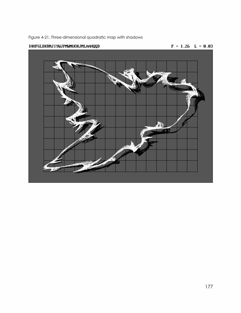
Figure 4-21. Three-dimensional quadratic map with shadows
177

Figure 4-22. Three-dimensional quadratic map with shadows
178

Figure 4-23. Three-dimensional quadratic map with shadows
179

Figure 4-24. Three-dimensional quadratic map with shadows
180
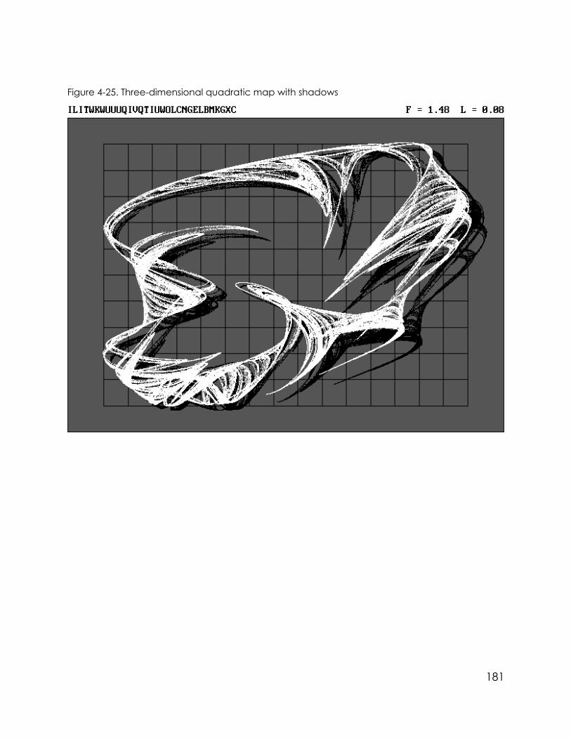
Figure 4-25. Three-dimensional quadratic map with shadows
181

Figure 4-26. Three-dimensional quadratic map with shadows
182

Figure 4-27. Three-dimensional quadratic map with shadows
183

Figure 4-28. Three-dimensional quadratic map with shadows
184

Figure 4-29. Three-dimensional quadratic map with shadows
185

Figure 4-30. Three-dimensional cubic map with shadows
186

Figure 4-31. Three-dimensional quartic map with shadows
187

Figure 4-32. Three-dimensional quartic map with shadows
188
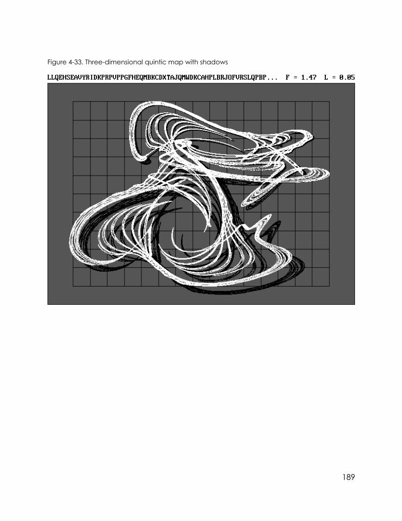
Figure 4-33. Three-dimensional quintic map with shadows
189
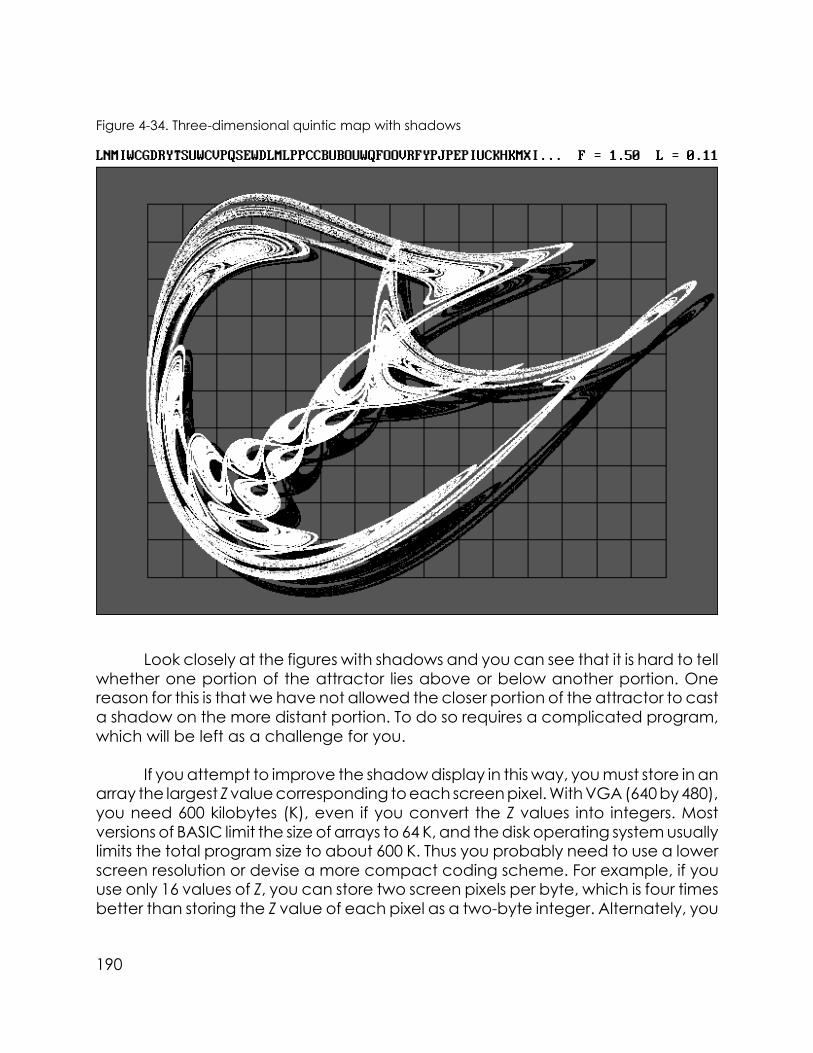
Figure 4-34. Three-dimensional quintic map with shadows
Look closely at the figures with shadows and you can see that it is hard to tellwhether one portion of the attractor lies above or below another portion. Onereason for this is that we have not allowed the closer portion of the attractor to casta shadow on the more distant portion. To do so requires a complicated program,which will be left as a challenge for you.
If you attempt to improve the shadow display in this way, you must store in anarray the largest Z value corresponding to each screen pixel. With VGA (640 by 480),you need 600 kilobytes (K), even if you convert the Z values into integers. Mostversions of BASIC limit the size of arrays to 64 K, and the disk operating system usuallylimits the total program size to about 600 K. Thus you probably need to use a lowerscreen resolution or devise a more compact coding scheme. For example, if youuse only 16 values of Z, you can store two screen pixels per byte, which is four timesbetter than storing the Z value of each pixel as a two-byte integer. Alternately, you
190

might store the Z values of only those pixels that are illuminated, but then you mustdevise a quick way to locate the proper element in the array corresponding toeach pair of screen coordinates.
Before each point on the attractor is plotted, you must be sure it doesn’t fallin the shadow of a previously plotted point. If it doesn’t, then it can be plotted, butthen you have to determine whether it occludes any previously plotted point.Alternatively, you can first plot all the points and then scan the image starting fromthe side toward the illumination, blocking out any points that fall in the shadow ofanother point.
4.3 Bands
Another way to display the third dimension is with elevation contours such asthose found on topographic maps. With enough points, you could plot only thosethat have specific values of Z. Of course the chance that a point has any particularexact value of Z is negligibly small, and so the points would accumulate on thescreen very slowly. To make the method work, you have to plot all the points thatlie within bands centered on the desired values.
You have freedom to choose the width of the bands. With narrow bands, thecontours resemble distinct lines, but they form very slowly. With wide bands, thegaps between the bands are hard to see. By making the bands half as wide as thespacing between the contours, the bright and dark spaces are equal in width, andthey form rapidly and are easy to see.
You also need to decide how many contours to use. You need at least severalto make the method work, but if you use too many, they begin to run together atmodest screen resolution and number of iterations. For the cases shown here, weuse 15 bands as a reasonable compromise.
Since we used a four-level gray scale to produce the shadows in the previousdisplays, we will also use it here to give the bands a softer shading. Of course, thisrequires a computer with at least EGA graphics. If your computer has CGA graphics,you will see only two shades (black and white) with 30 bands in SCREEN mode 2.
The changes required in the program to produce contour bands are shownin PROG13.
191

PROG13. Changes required in PROG12 to display contour bands
1000 REM THREE-D MAP SEARCH (With Contour Bands)
1120 TRD% = 2 'Display third dimension as bands
3760 IF Q$ = "R" THEN TRD% = (TRD% + 1) MOD 3: T% = 3: IF N > 999 THEN N = 999
4490 IF TRD% = 2 THEN PRINT "bands "
5130 IF TRD% = 2 THEN PSET (XP, YP), COLR%(INT(60 * (Z - ZMIN) / (ZMAX - ZMIN)+ 4) MOD 4)
5240 RETURN
Some sample attractors with contour bands produced by PROG13 are shownin Figures 4-35 through 4-50.
192

Figure 4-35. Three-dimensional quadratic map with contour bands
193

Figure 4-36. Three-dimensional quadratic map with contour bands
194

Figure 4-37. Three-dimensional quadratic map with contour bands
195
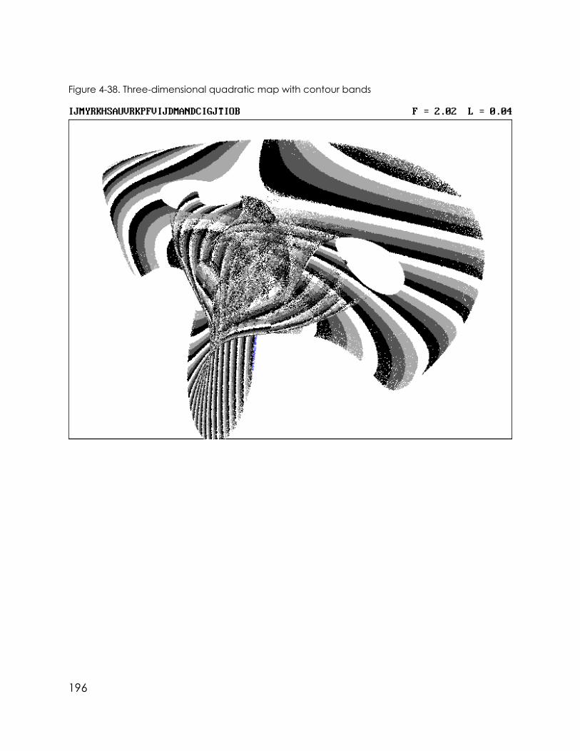
Figure 4-38. Three-dimensional quadratic map with contour bands
196
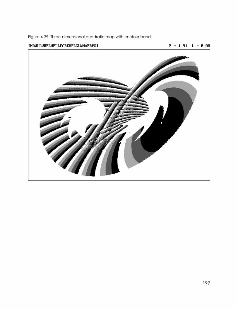
Figure 4-39. Three-dimensional quadratic map with contour bands
197
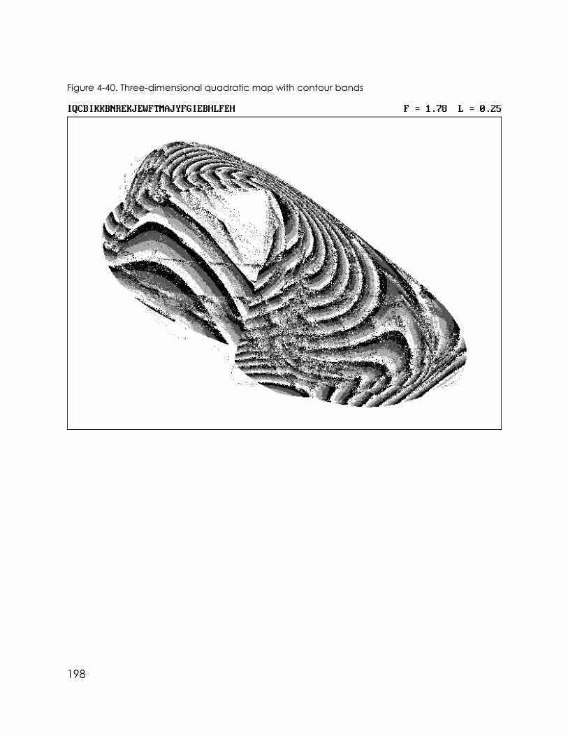
Figure 4-40. Three-dimensional quadratic map with contour bands
198

Figure 4-41. Three-dimensional quadratic map with contour bands
199

Figure 4-42. Three-dimensional cubic map with contour bands
200

Figure 4-43. Three-dimensional cubic map with contour bands
201

Figure 4-44. Three-dimensional cubic map with contour bands
202

Figure 4-45. Three-dimensional quartic map with contour bands
203

Figure 4-46. Three-dimensional quartic map with contour bands
204

Figure 4-47. Three-dimensional quartic map with contour bands
205

Figure 4-48. Three-dimensional quintic map with contour bands
206
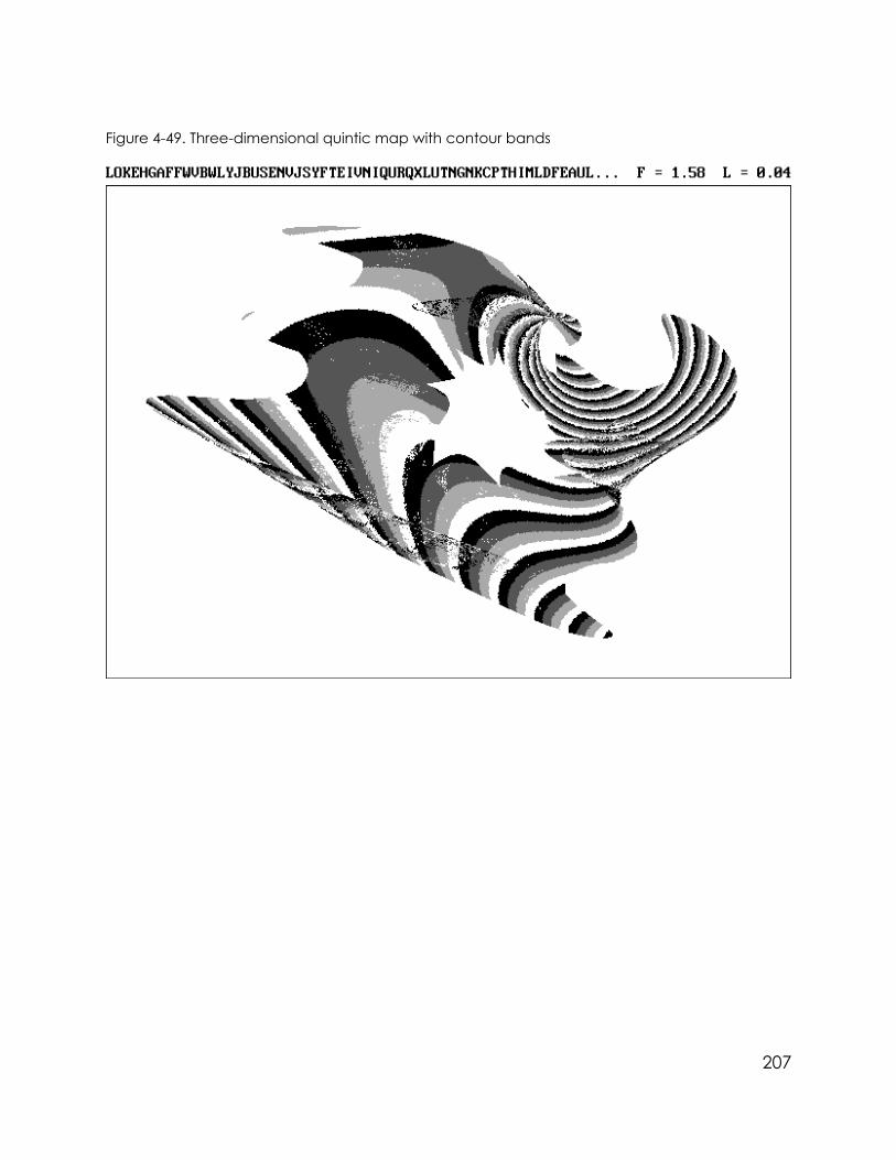
Figure 4-49. Three-dimensional quintic map with contour bands
207

Figure 4-50. Three-dimensional quintic map with contour bands
4.4 Colors
It’s not hard to guess that the next logical step is to use the full array of colorsavailable on a computer with a color monitor. In SCREEN mode 9 (EGA) and SCREENmode 12 (VGA), 16 colors can be displayed simultaneously from a palette of 64(EGA) or 262,144 (VGA). SCREEN mode 13 (VGA), which is supported by some BASICversions, allows 256 colors, but the screen resolution of 320 by 200 is inadequate forour purposes, and thus it will not be used. In SCREEN mode 1 (CGA) only four colorscan be displayed from one of two palettes. We assume your computer has EGA orVGA capabilities, but the program also works with CGA if you use SM% = 1 in line1030. The program is written to simplify extending the technique to future newgraphics modes with more colors and higher resolution, provided they are sup-ported by your BASIC compiler.
208
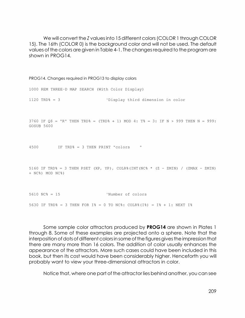
We will convert the Z values into 15 different colors (COLOR 1 through COLOR15). The 16th (COLOR 0) is the background color and will not be used. The defaultvalues of the colors are given in Table 4-1. The changes required to the program areshown in PROG14.
PROG14. Changes required in PROG13 to display colors
1000 REM THREE-D MAP SEARCH (With Color Display)
1120 TRD% = 3 'Display third dimension in color
3760 IF Q$ = "R" THEN TRD% = (TRD% + 1) MOD 4: T% = 3: IF N > 999 THEN N = 999:GOSUB 5600
4500 IF TRD% = 3 THEN PRINT "colors "
5160 IF TRD% = 3 THEN PSET (XP, YP), COLR%(INT(NC% * (Z - ZMIN) / (ZMAX - ZMIN)+ NC%) MOD NC%)
5610 NC% = 15 'Number of colors
5630 IF TRD% = 3 THEN FOR I% = 0 TO NC%: COLR%(I%) = I% + 1: NEXT I%
Some sample color attractors produced by PROG14 are shown in Plates 1through 8. Some of these examples are projected onto a sphere. Note that theinterposition of dots of different colors in some of the figures gives the impression thatthere are many more than 16 colors. The addition of color usually enhances theappearance of the attractors. More such cases could have been included in thisbook, but then its cost would have been considerably higher. Henceforth you willprobably want to view your three-dimensional attractors in color.
Notice that, where one part of the attractor lies behind another, you can see
209

the more distant portion through the closer portion. Thus the attractor appearstransparent, which enables you to see its interior but tends to diminish the percep-tion of depth. You might want to modify the program so that the closer portionoccludes the region behind it. It is relatively easy to do so using the BASIC POINTfunction to test the existing color of the pixel before plotting the new point andplotting it only if its color is higher in the sequence than the existing one. Thus eachpixel eventually is colored according to the closest part of the attractor. This effectcan be accomplished by changing line 5160 of PROG14 to
5160 IF TRD% = 3 THEN C% = INT(NC% * (Z - ZMIN) / (ZMAX - ZMIN) + NC%) MOD NC%:IF POINT(XP, YP) < C% THEN PSET (XP, YP), C%
You can also alter the sequence of colors by changing the values stored inthe array COLR% in line 5630. For example, a sequence that mimics the rainbowwould advance from red (12) through yellow (14), green (10), cyan (11), and blue(9) to magenta (13). With aerial perspective, brilliant, warm colors such as redappear closer to the viewer than lighter, less brilliant, cool colors such as blue, whichwe associate with the distant sky. Thus assigning red to the large Z values and blueto the small Z values enhances the illusion of depth.
Most dialects of BASIC include a PALETTE command that allows you tochange the screen colors without replotting the data, but this command worksdifferently with different versions of BASIC and in different graphics modes, so we willnot try to provide a program that takes advantage of it. However, a challengingprogramming exercise is to add the capability of rotating the color palette bypressing a key while a color attractor is being displayed to produce a psychedelicanimated display. You might use the + key to rotate in one direction and the - keyto rotate in the opposite direction. For most of the figures in this book, the PALETTEcommand was used to interchange black and white before printing them to saveink and to improve the appearance of the attractors when they are displayed ona white background.
You may also want to experiment with combining the various display tech-niques. Clearly there is nothing to preclude displaying a color attractor withshadows and contour bands. Such combinations offer interesting possibilities thatare exploited for the four-dimensional cases in the next chapter.
210

4.5 Characters
Many computer monitors and printers lack color capabilities. However, it isoften possible to produce a similar effect using a gray scale. In some cases, thevarious colors are mapped automatically into a shade of gray. Another techniquethat works on almost any computer and offers interesting display possibilities is tomap the Z values into different ASCII characters and print them as a block of text.Such text files are easily manipulated by word processors, transported to differentcomputers, displayed on almost any monitor, and printed with any printer on paperof various sizes.
Perhaps the simplest method is to map the Z values into consecutive ASCIIcharacters, thereby producing a type of gray scale with bands whose darknessdepends on the density of the character. A more reasonable approach is to orderthe characters so that the more dense ones correspond to larger values of Z. Theordering depends on the font, typeface, and size of the characters. For example,10-point Letter Gothic bold can be ordered as shown in Table 4-2. The table uses 32characters, which is about the maximum for this technique because many of thecharacters have the same density. The eye can distinguish about 500 levels of gray.This sequence is only one of many that are equally good. To see the gray scale, youshould view the table from at least six feet away. Squinting and removing yourglasses, if you wear them, might also help.
Table 4-2. Gray scale produced by ordering 10-point Letter Gothic bold characters
.:,;"=>!/+?icl7IjvJL64VOASUDXEBM
.:,;"=>!/+?icl7IjvJL64VOASUDXEBM
.:,;"=>!/+?icl7IjvJL64VOASUDXEBM
.:,;"=>!/+?icl7IjvJL64VOASUDXEBM
.:,;"=>!/+?icl7IjvJL64VOASUDXEBM
.:,;"=>!/+?icl7IjvJL64VOASUDXEBM
.:,;"=>!/+?icl7IjvJL64VOASUDXEBM
.:,;"=>!/+?icl7IjvJL64VOASUDXEBM
.:,;"=>!/+?icl7IjvJL64VOASUDXEBM
.:,;"=>!/+?icl7IjvJL64VOASUDXEBM
211

.:,;"=>!/+?icl7IjvJL64VOASUDXEBM
.:,;"=>!/+?icl7IjvJL64VOASUDXEBM
.:,;"=>!/+?icl7IjvJL64VOASUDXEBM
.:,;"=>!/+?icl7IjvJL64VOASUDXEBM
The character densities for this table were determined by writing each of theASCII characters from 33 to 127 (see Table 2-1) to the screen of a Macintoshcomputer and then counting the illuminated pixels using the POINT command inBASIC. Bold characters are chosen for their increased density. Avoid lowercasecharacters whenever possible because they often don’t extend the full height andthus leave a wide blank band between their top and the bottom of the row above.Be sure to use a monospaced font rather than a proportional one. For the defaultfont on most IBM computers in VGA SCREEN mode 12, a better sequence is
.-,;=+>i%lI?v7zuCjTFSVGAEUDHBWQ
We will not develop a computer program for implementing this techniquebecause the resolution is too poor for useful display on a computer screen or pageof a book. Furthermore, the program would be dependent on the fonts availableand the capabilities of the printer. The programming is not difficult and closelyparallels the example in PROG14.
However, Table 4-3 provides an indication of what is possible using 5-pointLetter Gothic bold characters with 78 lines of 103 characters each. The charactersequence ordered by density for this case is given in Table 4-2. This case is a three-dimensional quadratic map with a code of ILRRHAEYWNTPWFLHTCSLYLFAKQITQTW.
At such a low resolution, much of the detail is lost. However, if you have aprinter or plotter capable of printing small fonts on a large piece of paper, you canrecover the resolution and produce figures of considerable artistic quality. You candivide the text into many segments on separate pages and tape them together, orprint them on a paper roll or fanfold paper to make a very skinny attractor many feetlong. With ordinary objects such as the text in this book, extreme stretching in onedimension just produces sticklike figures. However, strange attractors are fractals,
212

and they have detail on all scales, which ensures that they look interesting howevermuch they are stretched.
Table 4-3. Three-dimensional quadratic map with character scale
::::..
; ::::
;;;;;;;
""""""""""""";
================
>>>==>>>>>>>!!!!!!
!>>>>!!!!////////////
JJ !!!!!!///++++++++++++++++
J //////++++++??iiiiiiiii??????
JJ +///++???? icccccccciccciiiiiiii
JJv ++++??ii? ccllllllllllllllccccccccii
JJv ??+??iiii lll777777777777lllllllllccccc
JJJj ????iicci 7777777IIIII777777777777llllllccc
JJv ii?iiccc IIIIIIIIIIIIIIIIIIIIIIII7777777lllllc
JJvj ciiiclll IIjjjjjjjjjjjjjjjjjjjjIIIIIIII777777lllll
JLvjj cccicclll jjjjjjjvvvvvvvvvvvjjjjjjjjjjjjjIIIIII77777lll
LLvjI llcccl777 jvvvvvvvvvvvvvvvvvvvvvvvvvvvvjjjjjjjjIIIIII7777l
LLvjjI77lllcll777 vvvvvvvJJJJJJJJJJJJJJJJJvvvvvvvvvvvvjjjjjjjIIIII777
LLvvjjI77llll77I7 vJJJJJJJJJJJJJJJJJJJJJJJJJJJJJJJJvvvvvvvvjjjjjjIIIII7
213

JLLvjjII77lll7III JJJJJJJJJJLLLLLLLLLLLLLLLLLJJJJJJJJJJJJJvvvvvvvjjjjjIIII7
LLvvjjII77777IjI JJJJJLLLLLLLLLLLLLLLLLLLLLLLLLLLLLLLLJJJJJJJJJvvvvvvjjjjjII
LLvvjjjII7777Ijj JJLLLLLLLLLLL LLLLLLLLLLLL6LLLLLLLLLLLLLLLLLJJJJJJJJvvvvvjjjjI
JLLvvjjIII77IIjjj LLLLLLL 6666666666666LLLLLLLLLLJJJJJJJvvvvvjj
LLvvvjjIIIIIIjvj LLLLL 66666666666666LLLLLLLLJJJJJJvvvvj
LLJvvjjjIIIIjjvv LLLLL 66666666666666LLLLLLLJJJJJJvv
LLvvvjjjjIIjjvv LLL 664446666666666LLLLLLJJJJ
LLJvvvjjjjjjjvvv L66 4444444466666666LLLLLLJ
JLJvvvvjjjjjvvJJ 6666 444444444446666666LLL
LLJvvvvvjjjvvJJ 666 4VV444444444466666
JLJJvv vvvvvvJJJ 66 VVVVVVV44444444
LLJJvv vvvvvJJJ 66 VVVVVVVVVVV444
JLJJJv vvvvJJJJ OOOOOVVVVVVVV
LLJJJv vJJJJL OOOOOOOOOOOOOOOOVV
LJJJJ JJJJLL AAAAAAAAAAAAAOOOOOOOOOOV
JJJJJJ JJJLL OOOOOOOOO AAAAAAAAAAAAAAAAAAAAAAAAAAAAAAAAAAOO
JJJJJ LLLL OOOOOOOOOOOOOAAAAAAAAAAAAAAAAAAAAAAAAAAAAAAAAAAAAAAAA
JJJJJ LLL OOOOOAAAAAAAAAAAAAAAAAAAAAASSASAASSSSSSSSAAAAAAA
JJJJJJ LLL AAAAAAAAAAAAASSSSSSSSSSSSSSSSSSSSSSSSSSSS
JJJJJJ LLL AAAAAASSSSSSSSSSSSSSSSSSSSSSSSSSSSSSSS
JJJJJJ L66 AASSSSSSSSSSSSSSSSSSSSSSSSSSSSSSSSSSS
JJJJJJ 66 ASSSSSSSSSSSSSSSUUUUUUUUUUUUUUUUUUUU
JJJJJJ 66 SSSSSSSSSSUUUUUUUUUUUUUUUUUUUUUUUU
214

LJJJJLL 6 SSSSSSUUUUUUUUUUUUUUUUUUUUUUUUUUU
LJJJLLL SSUUUUUUUUUUUUUUUUUUUUDDDDDDDDDDD
LLJLLLLL SUUUUUUUUUUUUUUDDDDDDDDDDDDDDDDD
LLJLLLLL UUUUUUUUUUDDDDDDDDDDDDDDDDDDDDD
LLLLLLLL UUUUUUDDDDDDDDDDDDDDDDDDDDDDDD
LLLLLLLLL UUUDDDDDDDDDDDDDDDDDXXXXXXXXXX
LLLLLLLLL UDDDDDDDDDDDDDDXXXXXXXXXXXXXX
LLLLLLLLL DDDDDDDDDDDXXXXXXXXXXXXXXXXXX
LLLLLLLL66 SS DDDDDDDDXXXXXXXXXXXXXXXXXXXX
LLLL6666666 SSSS DDDDDXXXXXXXXXXXXXXXXXEEEEEE
LLL666666444444 SSSS DXXXXXXXXXXXXXXEEEEEEEEEEEE
LLL666666444444VV SSSSS XXXXXXXXXXXXEEEEEEEEEEEEEE
LLL666664446644 SSSSS XXXXXXXXXEEEEEEEEEEEEEEEEE
LLL666666 SSSUU XXXXXXEEEEEEEEEEEEEEEBBBB
LLL6666 SUUUUU XXXXEEEEEEEEEEEEEBBBBBBBB
LLL66 O SUUUUUUU XXEEEEEEEEEEEEBBBBBBBBBB
LLLLL OO UUUUUUUUD EEEEEEEEEEEBBBBBBBBBBBBB
LLL OOO UUUUUUUUDDD EEEEEEEEBBBBBBBBBBBBBBB
LLLL OOOO SUUUUUUUDDDDDDD EEEEEEBBBBBBBBBBBBBMMM
LLLLLLL VOOOO SUUUUUUUDDDDDDDDXX EEEEEBBBBBBBBBBBBMMMMM
LLLLL6666664444444VVVVVOOOO SUUUUUUUUDDDDDDDDXXXXXX EEEBBBBBBBBBBBMMMMMMM
LLLLL6666664444444VVVVVOOO SSUUUUUUUUDDDDDDDXXXXXXXXXEEE EEBBBBBBBBBBBMMMMMMMM
LLLL6666666444444VVVVVVOO SSUUUUUUUDDDDDDDDXXXXXXXXEEEEEEEEEBBBBBBBBBBMMMMMMMMM
215

LLLLL666666444444VVVVVVOO SSSUUUUUUUDDDDDDDDXXXXXXXXEEEEEEEEEBBBBBBBBBMMMMMMMM
LLLL666666444444VVVVVVOOO SSSSUUUUUUUDDDDDDDDXXXXXXXEEEEEEEEEBBBBBBBBBBMMMMM
LL666666444444VVVVVVOOO SSSSUUUUUUUDDDDDDDXXXXXXXXEEEEEEEEBBBBBBBBBB
L66666644444VVVVVVOOOO SSSSSUUUUUUUDDDDDDDXXXXXXXXEEEEEEEEBBB
6666444444VVVVVVOOOO SSSSSSUUUUUUUDDDDDDDXXXXXXXXEEEEEEE
444444VVVVVVOOOOO ASSSSSSUUUUUUUDDDDDDDXXXXXXXEEEE
4VVVVVVOOOOOO AAASSSSSSUUUUUUUDDDDDDDXXXXXXXX
VVVOOOOOOOAAAAAASSSSSSUUUUUUUDDDDDDDXXXXX
VOOOOOOAAAAAASSSSSSUUUUUUUDDDDDDDXXX
OOOAAAAAASSSSSSSUUUUUUDDDDDDDD
AAAAAASSSSSSSUUUUUUDDDDD
AAASSSSSSSUUUUUUDDD
SSSSSUUUUUU
4.6 Anaglyphs
An alternative approach for displaying objects in three dimensions is thebinocular stereogram in which the parallax produced by separate images in eacheye creates the illusion of depth. The idea dates back to Socrates in the fourthcentury BC, and the earliest stereograms were produced in the mid-1800s by SirCharles Wheatstone and Sir David Brewster. The inception of motion pictures in theearly 1900s was accompanied by 3-D movies using overlapping red-green imagesthat were viewed through red-green glasses to produce a black-and-white imagein what is called the anaglyphic process. Anaglyphs have also been widely used incomic books. Color 3-D movies using cross-Polaroid glasses were briefly popular inthe 1950s. They require a special screen to reflect the polarized light from theprojectors without allowing it to depolarize.
The anaglyphic process offers distinct advantages in computer visualization.The hardware requirements are minimal (a color monitor and a pair of 50-cent
216
glasses), the programming is surprisingly simple, and the results can be impressive.The main drawback is that the images produced are usually monochromatic,although a gray scale and some limited coloration are possible.
Our perception of depth arises from a number of psychological and physi-ological processes. Many of these processes are induced by visual cues that don’tdepend on binocular vision, such as the relative size and motion of objects,interposition, illumination, shadows, and focal accommodation. Others require theparallax attendant to stereoscopic vision. When some of the usual visual cues areabsent or contradictory, a rivalry ensues that demands time and mental effort forour brains to resolve. It is remarkable that, with just the single cue of binocularstereopsis, most people can quickly perceive a vivid three-dimensional image.
Consider a point at a distance D from the midpoint of your eyes whoseseparation we take to be e (typically 6.5 cm), as shown in Figure 4-51(a). Assumethe point is a single illuminated pixel on the computer screen. Each eye must swivelinward through an angle θ in order for the two images to fuse into a single point,where θ is the angle whose tangent is e / 2D. It is this muscular response of the eyesthat provides the brain with the relevant depth information.
217

Figure 4-51. Line of sight of each eye when viewing anaglyphs
Now suppose you are to perceive the point to be at a distance D - Z from youreyes (a distance Z in front of the computer screen) as shown in Figure 4-51 (b). Wemust then plot two points on the computer screen separated horizontally by adistance d. From the similarity of the two triangles, we calculate
d = eZ / (D-Z) (Equation 4C)
The formula works also for negative Z.
To achieve the proper linear perspective, we should plot the closer points a
218

little farther apart than the more distant points, but with unfamiliar objects such asstrange attractors, there is little reason to do so. Usually D is much greater that Z, andwe can approximate the right-hand side of Equation 4C by e Z / D. This approxima-tion causes some expansion of the image for negative Z (behind the screen) andcompression of the image for positive Z (in front of the screen). This compression canbe desirable to keep the image always in front of your face rather than to let it passbehind your head.
The length of most people’s arms is almost exactly ten times the distancebetween their eyes. Therefore, a value of D / e = 10 is appropriate for a computerscreen viewed at arm’s length. In practice, the viewing distance is not very critical.The perceived depth of the image is enhanced by viewing from a greater distance,but it usually takes longer for the brain to accommodate, so it is often best to viewfirst from close up. It sometimes speeds the adjustment to move your head from sideto side.
A computer display optimized for viewing at arm’s length is very effectivewhen projected on a large screen and viewed in an auditorium. Were this not thecase, three-dimensional movies could not be shown to theater audiences. In sucha case, the brain perceives a scaled version of the image at a closer distance. Thesame effect occurs when viewing 2-D movies. The characters on the screen are notperceived as giants a large distance from the viewer. Similarly, the brain is able tocompensate almost without limit to other distortions if the objects are familiar. Amovie viewed from the rightmost seat in the front row appears normal after a shortperiod of adjustment.
It is important to maintain a somewhat limited depth and field of view.Leonardo da Vinci recommended that a painting be optimally viewed from adistance equal to three times its width. Most computer screens approximatelysatisfy this criterion when viewed at arm’s length. An object as deep as it is wide thusrequires that the two images be separated by up to about an inch, requiring thatthe eyes toe-in by about three degrees.
The computational task, therefore, is to plot each point that makes up theattractor twice, with a horizontal separation proportional to the distance the pointis to appear in front of or behind the screen, and to arrange that one set of pointsbe visible only to the left eye and the other only to the right eye. In the anaglyphicprocess, this is done by plotting one set of points in red and the other in thecomplementary cyan (blue-green) and viewing through appropriate color-filteredglasses. By convention, the left eye should only respond to the red and the right eyeonly to the cyan.
219

Note that individuals who are color blind should experience no difficultybecause it is unnecessary (and indeed undesirable) to perceive the individualcolors; it is only necessary that the eyes be sensitive to them. Certain other eyedefects, particularly those resulting in ocular asymmetry, are more problematic.
You can plot the points on either a black or a white background. With a blackbackground, the images fuse into white (additive process), and with a whitebackground, the images fuse into black (subtractive process). The sense of Z isreversed with the choice of background. With a black background, the red is seenthrough the red filter on the left eye, while for a white background, red is seenthrough the cyan filter on the right eye. In practice the white background is usuallymore satisfactory, but you may want to try it both ways to see which works best foryou. Wherever a red and cyan point overlap, they should be plotted as a singleblack point if the background is white or as a single white point if the backgroundis black. The changes required to the program to produce such anaglyphs areshown in PROG15.
PROG15. Changes required in PROG14 to produce anaglyphs
1000 REM THREE-D MAP SEARCH (With Anaglyphic Display)
1120 TRD% = 4 'Display third dimension as anaglyph
3220 ZA = (ZMAX + ZMIN) / 2
3240 IF TRD% = 4 THEN LINE (XL, YL)-(XH, YH), WH%, BF
3760 IF Q$ = "R" THEN TRD% = (TRD% + 1) MOD 5: T% = 3: IF N > 999 THEN N = 999:GOSUB 5600
4510 IF TRD% = 4 THEN PRINT "anaglyph "
5170 IF TRD% <> 4 THEN GOTO 5240
220

5180 XRT = XP + XZ * (Z - ZA): C% = POINT(XRT, YP)
5190 IF C% = WH% THEN PSET (XRT, YP), RD%
5200 IF C% = CY% THEN PSET (XRT, YP), BK%
5210 XLT = XP - XZ * (Z - ZA): C% = POINT(XLT, YP)
5220 IF C% = WH% THEN PSET (XLT, YP), CY%
5230 IF C% = RD% THEN PSET (XLT, YP), BK%
5640 WH% = 15: BK% = 8: RD% = 12: CY% = 11
PROG15 assumes EGA or VGA graphics and a color monitor. If you have CGAgraphics, you can obtain satisfactory results in SCREEN mode 1, PALETTE 1 bychanging the colors in line 5640 to WH% = 3: BK% = 0: RD% = 2: CY% = 1.
Some sample anaglyphs are shown in Plates 9 through 16. Use the specialglasses included with the book. If these glasses are missing, you can probably finda suitable pair at a comic book store. If you have difficulty acclimating to theanaglyphs, try viewing them from close-up and then back away once you see theeffect. You may need some practice, especially because the attractors you areviewing are unfamiliar objects and they lack other depth clues. You might also tryreversing the glasses (red over right eye), which reverses in and out.
Because of the large variation of computer monitor colors and spectaclefilters, ghost images are common. Manipulation of the computer color palette is oflimited use because the monitor ultimately constructs its colors from three distinctphosphors (red, green, and blue). The usual problem is inadequate rejection of thegreen by the red filter, resulting in a red ghost image when viewed against a whitebackground. Suppression of the green by using only red and blue on a magentabackground eliminates this problem but yields poor contrast of the resulting image.In some cases, the ghost images can be suppressed by viewing through multiplepairs of glasses. You may want to adjust the intensity of the red, green, and blue, sothe images seen by each eye through the glasses have similar intensities.
221

4.7 Stereo Pairs | Stereo Pairs
Believe it or not, with a bit of practice, you can learn to view attractors instereoscopic 3-D without special glasses. For this purpose, we print the two imagesside-by-side in the same color instead of superimposed on one another in differentcolors as we did with the anaglyphs. This technique permits full-color displays, andwe will exploit this capability in the next chapter. For the moment, let’s consider onlymonochrome images.
First we develop the computer program necessary to produce the images.The images should not be separated more than the distance between your eyes,which for most people is about 6.5 cm. If the images are separated by a largerdistance, the eyes have to rotate outward beyond the normal parallel position,which at best is uncomfortable and at worst impossible. Such images are describedas being walleyed. However, if we reduce the images to a sufficiently small size onthe computer screen, the resolution is poor. Therefore, we will plot the images aslarge as possible and rely on the printer to reduce the size for comfortable viewing.If you prefer to sacrifice the resolution and view the attractors directly on the screen,the program is written to make it easy for you to do so. Alternately, your monitor mayhave an adjustment that allows you to shrink the width of the image.
PROG16 shows the changes required to produce such stereo pairs.
PROG16. Changes required in PROG15 to produce stereo pairs
1000 REM THREE-D MAP SEARCH (With Stereo Display)
1120 TRD% = 5 'Display third dimension as stereogram
3250 IF TRD% = 5 THEN LINE (XA, YL)-(XA, YH)
3320 IF PJT% = 1 AND TRD% < 5 THEN CIRCLE (XA, YA), .36 * (XH - XL)
3760 IF Q$ = "R" THEN TRD% = (TRD% + 1) MOD 6: T% = 3: IF N > 999 THEN N = 999:GOSUB 5600
222

4520 IF TRD% = 5 THEN PRINT "stereogram"
5240 IF TRD% <> 5 THEN GOTO 5280
5250 HSF = 2 'Horizontal scale factor
5260 XRT = XA + (XP + XZ * (Z - ZA) - XL) / HSF: PSET (XRT, YP)
5270 XLT = XA + (XP - XZ * (Z - ZA) - XH) / HSF: PSET (XLT, YP)
5280 RETURN
If you want to shrink the image for direct viewing from the computer screen,change the horizontal scale factor (HSF) in line 5250 from 2 to a larger value thatseparates the images by about 6.5 centimeters, or less if you are having troubleadapting to them.
Sample stereo pairs produced by this technique are shown in Figures 4-52through 4-67. You should hold them exactly horizontally, directly in front of your faceat a normal reading distance, and gaze into the distance until you see threeimages. The one in the middle should appear in 3-D, and the ones on each side,which you must train yourself to ignore, should be in 2-D.
223

Figure 4-52. Stereo pair of three-dimensional quadratic map
224
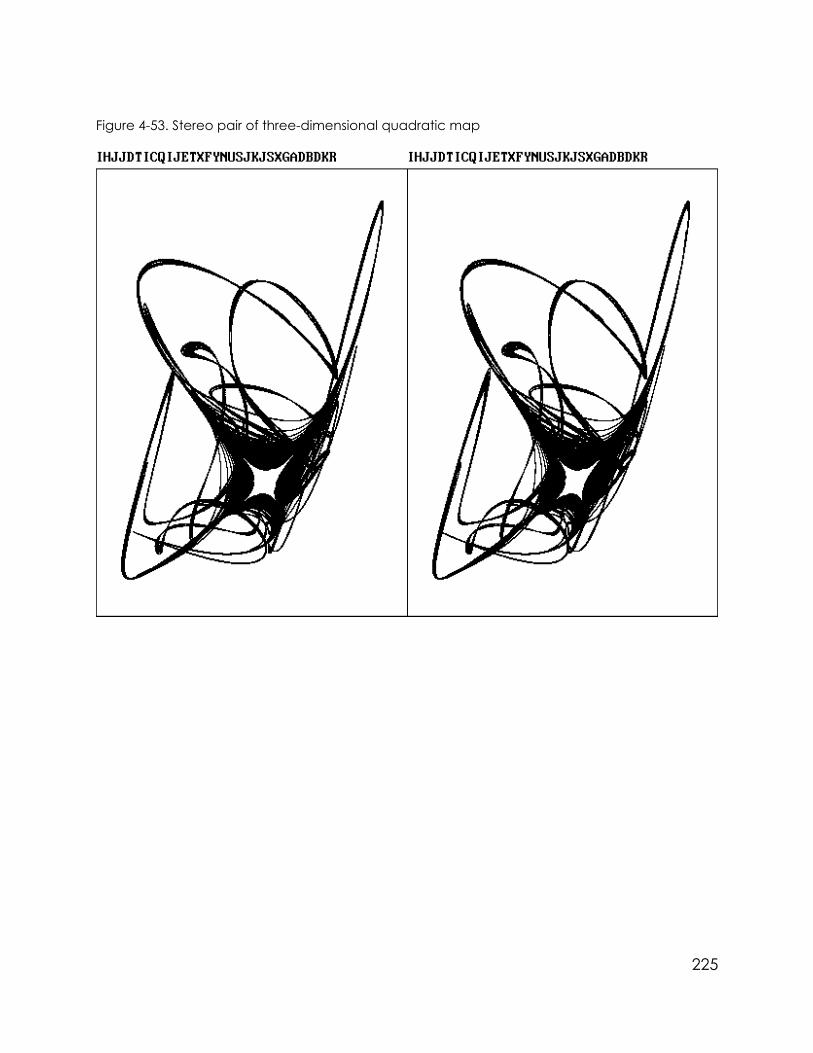
Figure 4-53. Stereo pair of three-dimensional quadratic map
225

Figure 4-54. Stereo pair of three-dimensional quadratic map
226

Figure 4-55. Stereo pair of three-dimensional quadratic map
227

Figure 4-56. Stereo pair of three-dimensional quadratic map
228

Figure 4-57. Stereo pair of three-dimensional quadratic map
229

Figure 4-58. Stereo pair of three-dimensional quadratic map
230
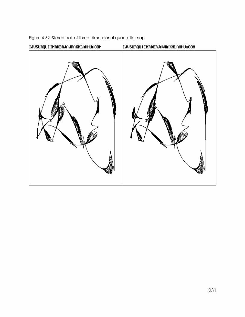
Figure 4-59. Stereo pair of three-dimensional quadratic map
231

Figure 4-60. Stereo pair of three-dimensional quadratic map
232

Figure 4-61. Stereo pair of three-dimensional quadratic map
233

Figure 4-62. Stereo pair of three-dimensional quadratic map
234

Figure 4-63. Stereo pair of three-dimensional cubic map
235

Figure 4-64. Stereo pair of three-dimensional cubic map
236
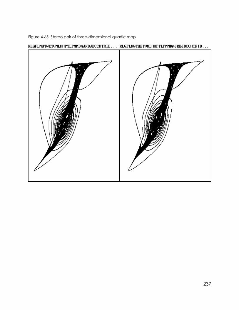
Figure 4-65. Stereo pair of three-dimensional quartic map
237

Figure 4-66. Stereo pair of three-dimensional quartic map
238

Figure 4-67. Stereo pair of three-dimensional quintic map
You may find it difficult to adjust to the images at first, but with practice youshould be able to see them almost instantly. Viewing them should be relaxing, witha sensation resembling a blank stare. Effort is required to return to normal viewing,much like returning to the words on this page after gazing into the distance.
It might help to close your eyes momentarily and then reopen them if you arehaving trouble adapting. You can also buy an inexpensive hand stereoscopecontaining prisms that separate and magnify the images so that you can view themfrom a closer distance. Such viewing forces the side images out of your field of viewand eases the adjustment to the middle image.
In the 1950s, the View-Master stereo viewer was very popular for home use,and many stereoscopic photographs were produced. Their popularity has waned,and the View-Master is no longer made, but similar inexpensive models can still be
239

found in toy stores, often with images of cartoon characters. Stereo images areusually photographed with a dual camera whose separation can be increasedbeyond the normal eye separation to enhance the depth sensation in what iscalled hyperstereo.
Stereoscopic images are used extensively by geologists and cartographersto determine terrain elevation from aerial photographs. As an airplane or satellitetravels across the Earth, photographs are taken at two positions separated by adistance much greater than the distance between the eyes. When viewed througha stereoscope, the Earth appears as a scaled model viewed from just a foot or soabove, and it is easy to discern the elevation changes.
The preceding technique is called free viewing. An alternate and moredifficult technique, called short-focus viewing, can also be used to view the stereopairs. Here the procedure is to place the figure at arm’s length but to look at a pointabout halfway to the figure. It may help to hold your finger at the halfway point andto cross your eyes until you see a single image of your finger. You should then seethe three images of the figure float up off the page in the plane of your finger. Themiddle image should be three-dimensional. It may be difficult to keep the imagefrom wavering and returning to the plane of the page. Squinting sometimes helps.
Some people find short-focus viewing easier than free viewing. If you areinstinctively short-foucus viewing, you will find that the right side of Figure 4-67 isfarther from you than the left side. With free viewing, it will be closer.
An advantage of short-focus viewing is that the images can be separated bya much larger distance, and so it works for projection on a large screen in aclassroom or auditorium. However, note that the image is in-out reversed from whatit is with free viewing. This reversal is called pseudostereo. With anaglyphs,pseudostereo can be obtained by reversing the glasses. Pseudostereo imagesusually would be very undesirable and would lead to all kinds of visual contradic-tions, but with our strange attractors, which have no other visual depth cues, itmakes little difference. It can even be an advantage to be able to view the objectsin either of these ways. Can you guess what you will see if you turn the figures upsidedown? Think about it, and then give it a try.
Note that with free viewing, the left image disappears when you close yourright eye and the right image disappears when you close your left eye. With short-focus viewing, the opposite occurs. However, it is incorrect to assume that each eyesees only one of the images. Both eyes see both images, and the images fuse intoone when your eyes are aimed in the proper direction.
240

4.8 Slices
We will discuss one final way to view attractors resulting from three-dimen-sional maps. Low-dimensional attractors are like loosely wound balls of string,whereas high-dimensional ones are more like loaves of bread filled with holes.Anaglyphs and stereo pairs are effective for cases of low dimension, but as thedimension increases, the attractor becomes too opaque, and the illusion of depthis lost.
Carrying the loaf-of-bread analogy a bit further, you could imagine slicingthe loaf into a large number of very thin slices. The result is to decrease the dimensionof the object by one. For example, an object with a fractal dimension of 2.5 wouldbecome an object of dimension of 1.5 in each slice. This is an example of what iscalled a Poincaré section (as in "cross section").
Perhaps it’s easier to consider a specific case. Suppose the attractor were aloosely wound ball of very thin string. The attractor would then be essentially one-dimensional. The string would cross the slices at a number of points. Thus the sliceswould contain dots wherever the string pierced them. A set of a finite number ofdots is an object of zero dimension.
If the attractor were a loosely crumpled piece of paper, its dimension wouldbe close to two. If you were to cut a thin slice through the crumpled paper, youwould be left with a handful of wormlike paper strings, which are one-dimensionalobjects. You should now set the book down, get a piece of paper and a pair ofscissors, and try it for yourself. Be sure to make the slice as thin as possible.
With our maps, which contain only a finite number of points, we cannot makethe slices too thin, lest they contain so few points as to be invisible. Furthermore, itis impractical to look at all the slices if they are very thin because there are too manyof them. As always, we have to compromise. We’ll use 16 slices and lay them outin a 4 by 4 array so that we can see them all at once. On the computer screen, thismethod entails a serious sacrifice in resolution, but it does illustrate the principle. Youmight want to experiment with using a larger number of slices but displaying only afraction of them. For example, try using 64 slices, and display every fourth one.
The modifications that are required to make the program produce a sliceddisplay are shown in PROG17.
241

PROG17. Changes required in PROG16 to produce slices
1000 REM THREE-D MAP SEARCH (With Sliced Display)
1120 TRD% = 6 'Display third dimension as slices
3260 IF TRD% <> 6 THEN GOTO 3310
3270 FOR I% = 1 TO 3
3280 XP = XL + I% * (XH - XL) / 4: LINE (XP, YL)-(XP, YH)
3290 YP = YL + I% * (YH - YL) / 4: LINE (XL, YP)-(XH, YP)
3300 NEXT I%
3760 IF Q$ = "R" THEN TRD% = (TRD% + 1) MOD 7: T% = 3: IF N > 999 THEN N = 999:GOSUB 5600
4530 IF TRD% = 6 THEN PRINT "slices "
5280 IF TRD% <> 6 THEN GOTO 5330
5290 DZ = (15 * (Z - ZMIN) / (ZMAX - ZMIN) + .5) / 16
5300 XP = (XP - XL + (INT(16 * DZ) MOD 4) * (XH - XL)) / 4 + XL
5310 YP = (YP - YL + (3 - INT(4 * DZ) MOD 4) * (YH - YL)) / 4 + YL
5320 PSET (XP, YP)
5330 RETURN
Figures 4-68 through 4-83 show some sample attractors displayed as asuccession of slices. The succession is from left to right and top to bottom in the same
242
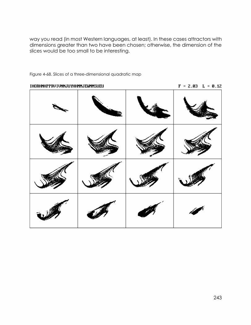
way you read (in most Western languages, at least). In these cases attractors withdimensions greater than two have been chosen; otherwise, the dimension of theslices would be too small to be interesting.
Figure 4-68. Slices of a three-dimensional quadratic map
243

Figure 4-69. Slices of a three-dimensional quadratic map
244
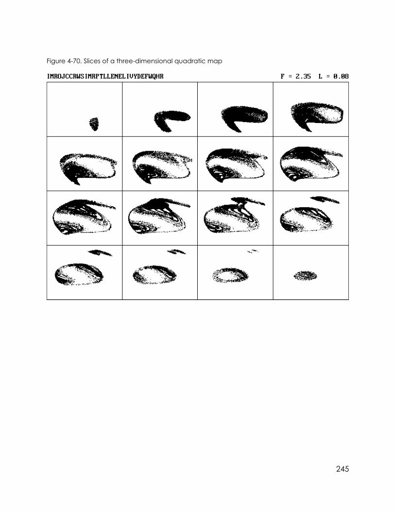
Figure 4-70. Slices of a three-dimensional quadratic map
245

Figure 4-71. Slices of a three-dimensional quadratic map
246
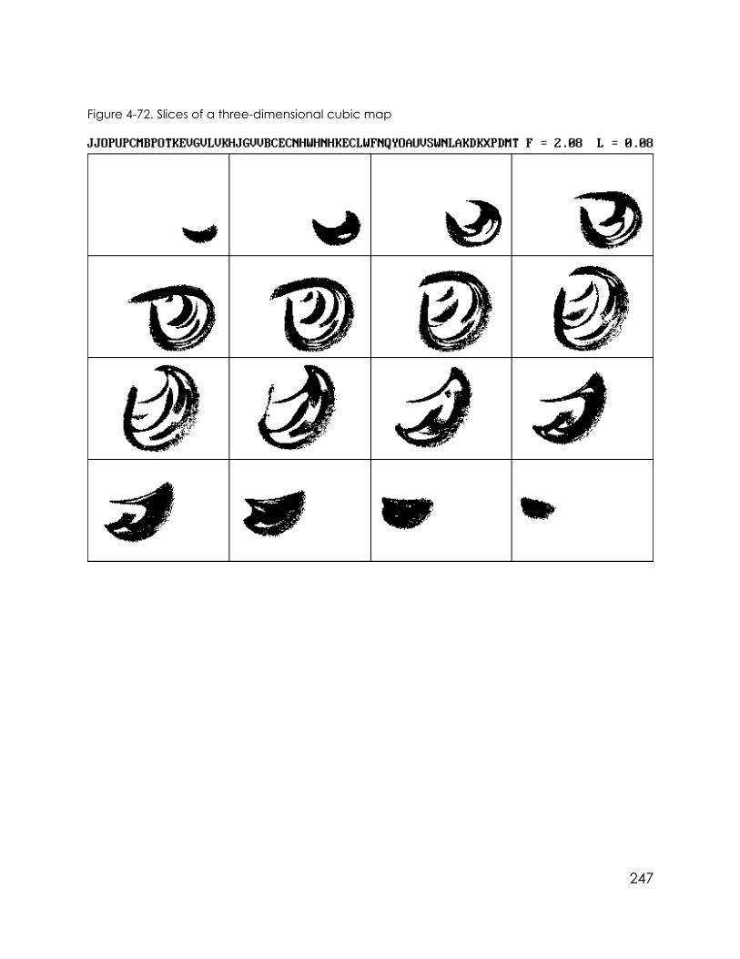
Figure 4-72. Slices of a three-dimensional cubic map
247

Figure 4-73. Slices of a three-dimensional cubic map
248

Figure 4-74. Slices of a three-dimensional cubic map
249

Figure 4-75. Slices of a three-dimensional cubic map
250

Figure 4-76. Slices of a three-dimensional quartic map
251

Figure 4-77. Slices of a three-dimensional quartic map
252

Figure 4-78. Slices of a three-dimensional quartic map
253

Figure 4-79. Slices of a three-dimensional quartic map
254

Figure 4-80. Slices of a three-dimensional quintic map
255

Figure 4-81. Slices of a three-dimensional quintic map
256
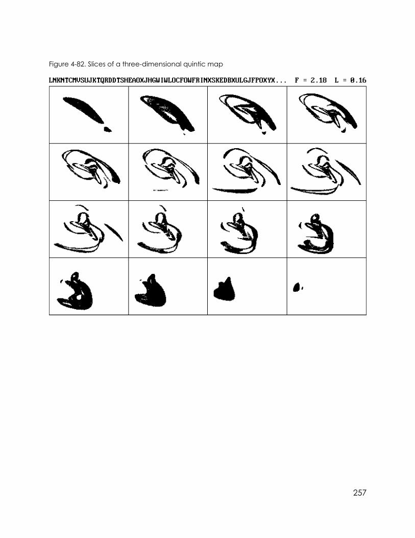
Figure 4-82. Slices of a three-dimensional quintic map
257
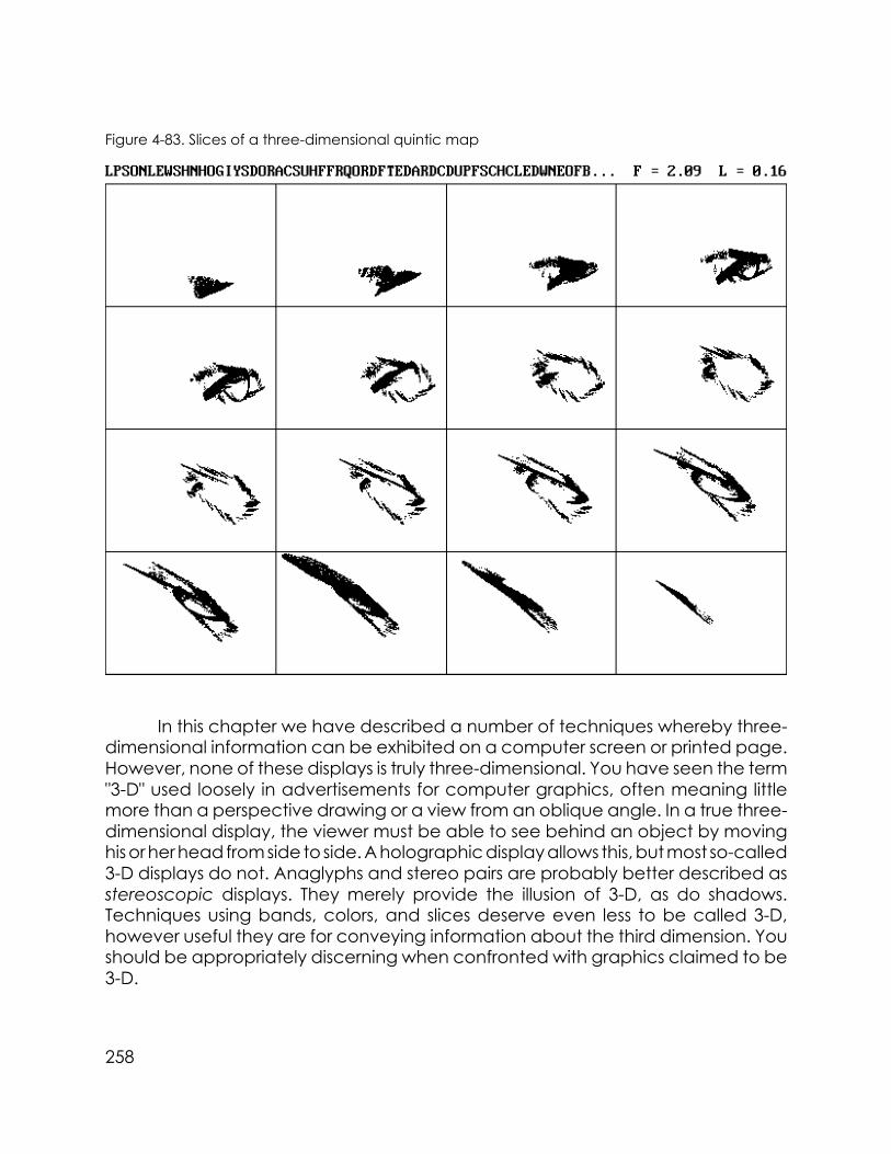
Figure 4-83. Slices of a three-dimensional quintic map
In this chapter we have described a number of techniques whereby three-dimensional information can be exhibited on a computer screen or printed page.However, none of these displays is truly three-dimensional. You have seen the term"3-D" used loosely in advertisements for computer graphics, often meaning littlemore than a perspective drawing or a view from an oblique angle. In a true three-dimensional display, the viewer must be able to see behind an object by movinghis or her head from side to side. A holographic display allows this, but most so-called3-D displays do not. Anaglyphs and stereo pairs are probably better described asstereoscopic displays. They merely provide the illusion of 3-D, as do shadows.Techniques using bands, colors, and slices deserve even less to be called 3-D,however useful they are for conveying information about the third dimension. Youshould be appropriately discerning when confronted with graphics claimed to be3-D.
258
Chapter 5The Fourth Dimension
Although we normally think of space as three-dimensional, mathematics isnot so constrained. Strange attractors can be embedded in space of four andeven higher dimensions. Their calculation is a straightforward extension of what wehave done before. The challenge is to find ways to visualize such high-dimensionalobjects. This chapter exploits a number of appropriate visualization techniquesafter a digression to explain why dimensions higher than three are useful fordescribing the world in which we live.
5.1 Hyperspace
Ordinary space is three-dimensional. The position of any point relative to anarbitrary origin can be characterized by a set of three numbers—the distanceforward or back, right or left, up or down. An object, such as a solid ball, in this spacemay itself be three-dimensional, or perhaps, like an eggshell of negligible thickness,it may be two-dimensional. You can also imagine an infinitely fine thread, which isone-dimensional, or the period at the end of this sentence, which is essentially zero-dimensional. Although we can easily visualize objects with dimensions less than orequal to three, it is hard to envision objects of higher dimension.
Before discussing the fourth dimension, it is useful to clarify and refine somefamiliar terms. Perhaps the best example of a one-dimensional object is a straightline. The line may stretch to infinity in both directions, or it may have ends. A lineremains one-dimensional even if it bends, in which case we call it a curve.
When we say that a curve is one-dimensional, we are referring to its topologi-cal dimension. By contrast the Euclidean dimension is the dimension of the spacein which the curve is embedded. If the line is straight, both dimensions are one, butif it curves, the Euclidean dimension must be higher than the topological dimensionin order for it to fit into the space. Both dimensions are integers. One definition of afractal is an object whose Hausdorff-Besicovitch (fractal) dimension exceeds itstopological dimension. For example a coastline on a flat map has a topologicaldimension of one, a Euclidean dimension of two, and a fractal dimension betweenone and two. It is an infinitely long line. On a globe, its Euclidean dimension wouldbe three.
259

A special and important example of a curve is a circle—a curve of finitelength but without ends, every segment of which lies at a constant distance froma point at the center. Every circle lies in a plane, which is a flat, two-dimensionalentity. Like a line, the plane may stretch to infinity in all directions, or it may haveedges. If a plane has an edge, we call it a disk. Note the distinction between a circle,which is a one-dimensional object that does not include its interior, and a circulardisk, which is a two-dimensional object that includes the interior.
Just as not all lines are straight, not all two-dimensional objects are flat. Asheet of paper of negligible thickness remains two-dimensional if it is curled or evencrumpled up, in which case it is no longer a plane but is still a surface. A curvedsurface has a Euclidean dimension of at least three. A surface can be finite butwithout edges. An example is a sphere, every segment of which is at a constantdistance from its center.
Note that just as a circle doesn’t include its interior, neither does a sphere.When we want to refer to the three-dimensional region bounded by a sphere, wecall it a ball. This terminology is universal among mathematicians, but not amongphysicists, who sometimes consider the dimension of circles and spheres to be theminimum Euclidean dimension of the space in which they can be embedded (twoand three, respectively).
Another example of a finite surface without edges is a torus, most familiar asthe surface of a doughnut or inner tube. Such curved spaces without edges areuseful whenever one of the variables is periodic. Spaces of arbitrary dimensions,whether flat or curved, are called manifolds. The branch of mathematics that dealswith these shapes is called topology.
If we could describe the world purely by specifying the position of objects,three dimensions would suffice. However, if you consider the motion of a baseball,you are interested not only in where it is, but in how fast it is moving and in whatdirection. Six numbers are needed to specify both its position and its velocity. Thissix-dimensional space is called phase space. Furthermore, if the ball is spinning, sixmore dimensions are needed, one to specify the angle and another to specify theangular velocity about each of three perpendicular axes through the ball.
If you have two spinning balls that move independently, you need a phasespace with twice as many (24) dimensions, and so forth. Contemplate the phase-space dimension required to specify the motion of more than 1025 molecules inevery cubic meter of air! Sometimes physicists even find it useful to performcalculations in an infinite-dimensional space, called Hilbert space.
260

You might also be interested in other properties of the balls, such as theirtemperature, color, or radius. Thus the state of the balls as time advances can bedescribed by a curve, or trajectory, in some high-dimensional space called statespace, in which the various perpendicular directions correspond to the quantitiesthat describe the balls. The trajectory is a curve connecting temporally successivepoints in state space.
You have probably heard of time referred to as the fourth dimension andassociate the idea with the theory of relativity. Long before Einstein, it was obviousthat to specify an event, as opposed to a location, it is necessary to specify not onlywhere the event occurred (X, Y, and Z) but also when (T). We can consider eventsto be points in this four-dimensional space.
Note that the spatial coordinates of a point are not unique. An object fourfeet in front of one observer might be six feet to the right of a second and two feetabove a third. The values of X, Y, and Z of the position depend on where thecoordinate system is located and how it is oriented. However, we would expect thevarious observers to agree on the separation between any two locations. Similarlywe expect all observers to agree on the time interval between two events.
The special theory of relativity asserts that observers usually do not agree oneither the separation or the time interval between two events. Events that aresimultaneous for one observer will not be simultaneous for a second moving relativeto the first. Similarly, two successive events at the same position as seen by oneobserver will be seen at different positions by the other.
You have probably heard that, according to the special theory of relativity,moving clocks run slow and moving meter sticks are shortened. (It is also true thatthe effective mass of an object increases when it moves, leading to the famousE = mc2, but that’s another story.) These discrepancies remain even after theobservers correct for their motion and for the time required for the informationabout the events to reach them traveling at the speed of light. It is important tounderstand that these facts have nothing to do with the properties of clocks andmeter sticks and that they are not illusions; they are properties of space and time,neither of which possess the absolute qualities we normally ascribe to them.
What is remarkable is that all observers agree on the separation between theevents in four-dimensional space-time. This separation is called the proper length,and it is calculated from the Pythagorean theorem by taking the square root of thesum of the squares of the four components after converting the time interval (∆T) toa distance by multiplying it by the speed of light (c). The only subtlety is that thesquare of the time enters as a negative quantity:
261

Proper length = [_X2 + _Y2 + _Z2 - c2_T2]1/2 (Equation 5A)
Because of the minus sign in Equation 5A, time is considered to be animaginary dimension; an imaginary number is one whose square is negative. Note,however, that the word "imaginary" does not mean it is any less real than the otherdimensions, only that its square combines with the others through subtraction ratherthan addition. If you are unfamiliar with imaginary numbers, don’t be put off by thename. They aren’t really imaginary; they are just the other part of certain quantitiesthat require a pair of numbers rather than a single number to specify them.
The minus sign also means that proper length, unlike ordinary length, may beimaginary. If the proper length is imaginary, we say the events are separated in atimelike, as opposed to a spacelike, manner. Timelike events can be causallyrelated (one event can influence the other), but spacelike events cannot, becauseinformation about one would have to travel faster than the speed of light to reachthe other, which is impossible. Events separated in a timelike manner are moreconveniently characterized by a proper time:
Proper time = [_T2 - _X2/c2 - _Y2/c2 - _Z2/c2]1/2 (Equation 5B)
In this case, time is real, but space is imaginary. Proper length is the length of anobject as measured by an observer moving with the same velocity as the object,and proper time is the time measured by a clock moving with the same velocity asthe observer.
Quantities such as proper length and proper time on which all observersagree, independent of their motion, are called invariants. The speed of light itselfis an invariant. There are many others, and they all involve four components thatcombine by the Pythagorean theorem.
Thus the theory of relativity ties space and time together in a very fundamen-tal way. One person’s space is another person’s time. Since space and time can betraded back and forth, there is no reason to call time the fourth dimension any morethan we call width the second dimension. It is better just to say that space-time is
262

four-dimensional, with each dimension on an equal footing. The apparent asym-metry between space and time comes from the large value of c (3 x 10⁸ meters persecond, or about a billion miles per hour) and the fact that time moves in only onedirection (past to future). It is also important to understand that, although specialrelativity is called a "theory," it has been extensively verified to high accuracy bymany experiments, most of which involve particle accelerators.
The foregoing discussion explains why it might be useful to consider four-dimensional space and four-dimensional objects, but it is probably fruitless to wastetoo much time trying to visualize them. However, we can describe them math-ematically as extensions of familiar objects in lower dimensions.
For example, a hypercube is the four-dimensional extension of the three-dimensional cube and the two-dimensional square. It has 16 corners, 32 edges, 24faces, and contains 8 cubes. Its hypervolume is the fourth power of the length ofeach edge, just as the volume of a cube is the cube of the length of an edge andthe area of a square is the square of the length of an edge.
A hypersphere consists of all points at a given distance from its center in four-dimensional space. Its hypersurface is three-dimensional and consists of an infinitefamily of spheres, just as the surface of an ordinary sphere is two-dimensional andconsists of an infinite family of circles. We have reason to believe that our Universemight be a hypersurface of a very large hypersphere, in which case we could seeourselves if we peered far enough into space, except for the fact that we are alsolooking backward to a time before Earth existed. We would also need an incrediblypowerful telescope to see Earth in this way. Thus our perception that space is three-dimensional could be analogous to the ancient view that Earth was flat, aconsequence of experience limited to a small portion of its surface.
5.2 Projections
The previous section was intended to motivate your consideration of strangeattractors embedded in four-dimensional space, but most of the discussion is notessential to what follows. We will now describe the computer program necessary toproduce attractors in four dimensions and then develop methods to visualize them.
The mathematical generalization from three to four dimensions is straightfor-ward. Whereas before we had three variables—X, Y, and Z—we now have a fourth.Having used up the three letters at the end of the alphabet, we must back up anduse W for the fourth dimension, but remember that all the dimensions are on an
263

equal footing. We use the first letters M, N, O, and P to code 4-D attractors of secondthrough fifth orders, respectively. The number of coefficients for these cases is 60,140, 280, and 504, respectively. The number of coefficients for order O is (O + 1)(O+ 2)(O + 3)(O + 4) / 6. The number of four-dimensional fifth-order codes is 25504, anumber too large to compare to anything meaningful; it might as well be infinite.
The program modifications required to add a fourth dimension are shown inPROG18.
PROG18. Changes required in PROG17 to add a fourth dimension
1000 REM FOUR-D MAP SEARCH
1020 DIM XS(499), YS(499), ZS(499), WS(499), A(504), V(99), XY(4), XN(4), COLR%(15)
1070 D% = 4 'Dimension of system
1120 TRD% = 0 'Display third dimension as projection
1540 W = .05
1550 XE = X + .000001: YE = Y: ZE = Z: WE = W
1610 WMIN = XMIN: WMAX = XMAX
1720 M% = 1: XY(1) = X: XY(2) = Y: XY(3) = Z: XY(4) = W
2010 M% = M% - 1: XNEW = XN(1): YNEW = XN(2): ZNEW = XN(3): WNEW = XN(4)
2180 IF W < WMIN THEN WMIN = W
2190 IF W > WMAX THEN WMAX = W
2210 XS(P%) = X: YS(P%) = Y: ZS(P%) = Z: WS(P%) = W
264

2410 IF ABS(XNEW) + ABS(YNEW) + ABS(ZNEW) + ABS(WNEW) > 1000000! THEN T% = 2
2470 IF ABS(XNEW - X) + ABS(YNEW - Y) + ABS(ZNEW - Z) + ABS(WNEW - W) < .000001THEN T% = 2
2540 W = WNEW
2910 XSAVE = XNEW: YSAVE = YNEW: ZSAVE = ZNEW: WSAVE = WNEW
2920 X = XE: Y = YE: Z = ZE: W = WE: N = N - 1
2950 DLZ = ZNEW - ZSAVE: DLW = WNEW - WSAVE
2960 DL2 = DLX * DLX + DLY * DLY + DLZ * DLZ + DLW * DLW
3010 ZE = ZSAVE + RS * (ZNEW - ZSAVE): WE = WSAVE + RS * (WNEW - WSAVE)
3020 XNEW = XSAVE: YNEW = YSAVE: ZNEW = ZSAVE: WNEW = WSAVE
3150 IF WMAX - WMIN < .000001 THEN WMIN = WMIN - .0000005: WMAX = WMAX + .0000005
3680 IF Q$ = "D" THEN D% = 1 + (D% MOD 4): T% = 1
3920 IF N = 1000 THEN D2MAX = (XMAX - XMIN) ̂ 2 + (YMAX - YMIN) ̂ 2 + (ZMAX - ZMIN)^ 2 + (WMAX - WMIN) ^ 2
3940 DX = XNEW - XS(J%): DY = YNEW - YS(J%): DZ = ZNEW - ZS(J%): DW = WNEW - WS(J%)
3950 D2 = DX * DX + DY * DY + DZ * DZ + DW * DW
4760 IF D% > 2 THEN FOR I% = 3 TO D%: M% = M% / (I% - 1): NEXT I%
If you run PROG18 under certain old versions of BASIC, such as BASICA andGW-BASIC, you are likely to get an error in line 2710 when the program attempts toconstruct a code for the fourth-order and fifth-order maps as a result of the string-length limit of 255 characters. In such a case, you may need to restrict the search
265
to second and third orders by setting OMAX% = 3 in line 1060. Alternatively, it’s notdifficult to modify the program to store the code in a pair of strings or to replace thestring with a one-dimensional array of integers containing the numeric equivalentsof each character in the string, perhaps with a terminating zero to signify the endof the string. For example, after dimensioning CODE%(504) in line 1020, line 2710would become
2710 CODE%(I%) = 65 + INT(25 * RAN)
and line 2740 would become
2740 A(I%) = (CODE%(I%) - 77) / 10
Also notice that the search for attractors is painfully slow unless you have avery fast computer and a good compiler. Refer back to Table 2-2, which lists someoptions for increasing the speed. The search can be made faster by limiting it tosecond order by setting OMAX% = 2 in line 1060.
We have another trick we can use to increase dramatically the rate at whichfour-dimensional strange attractors are found without sacrificing variety. It turns outthat most of these attractors have their constant terms near zero. The reasonpresumably has to do with the fact that the origin (X = Y = Z = W = 0) is then a fixedpoint, and the initial condition is chosen near the origin (X0 = Y0 = Z0 = W0 = 0.05).If the fixed point is unstable, then we have one of the conditions necessary forchaos. It is easy to accomplish this by adding after line 2730 a statement such as
2735 IF I% MOD M% / D% = 1 THEN MID$(CODE$, I% + 1, 1) = "M"
This increases the rate of finding attractors by about a factor of 50. Many of theattractors illustrated in this chapter were produced in this way. This change alsoincreases the rate for lower-dimensional maps, but by a much smaller factor. This
266

improvement suggests that there is yet room to optimize the search routine by amore intelligent choice of the values of the other coefficients.
Note that PROG18 does not attempt to display the fourth dimension butprojects it onto the other three, for which all the visualization techniques of the lastchapter are available. Don’t waste too much time trying to understand what itmeans to project a four-dimensional object onto a three-dimensional space. It is justa generalization of projecting a three-dimensional object onto a two-dimensionalsurface. In the program, it simply involves plotting X, Y, and Z and ignoring thevariable W.
Some examples of four-dimensional attractors projected onto the two-dimensional XY plane are shown in Figures 5-1 through 5-20. They don’t lookparticularly different from those obtained by projecting three-dimensional attractorsonto the plane or, indeed, by just plotting two-dimensional attractors directly. Notethat most of these attractors have fractal dimensions less than or about 2.0, soperhaps it is not too surprising that their projections resemble those produced byequations of lower dimension. It is rare to find attractors with fractal dimensionsgreater than 3.0 produced by four-dimensional polynomial maps, as will be shownin Section 8.1.
267

Figure 5-1. Projection of four-dimensional quadratic map
268
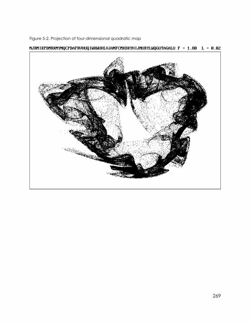
Figure 5-2. Projection of four-dimensional quadratic map
269

Figure 5-3. Projection of four-dimensional quadratic map
270

Figure 5-4. Projection of four-dimensional quadratic map
271

Figure 5-5. Projection of four-dimensional quadratic map
272

Figure 5-6. Projection of four-dimensional quadratic map
273

Figure 5-7. Projection of four-dimensional quadratic map
274

Figure 5-8. Projection of four-dimensional quadratic map
275

Figure 5-9. Projection of four-dimensional quadratic map
276

Figure 5-10. Projection of four-dimensional quadratic map
277

Figure 5-11. Projection of four-dimensional quadratic map
278

Figure 5-12. Projection of four-dimensional quadratic map
279

Figure 5-13. Projection of four-dimensional quadratic map
280

Figure 5-14. Projection of four-dimensional quadratic map
281
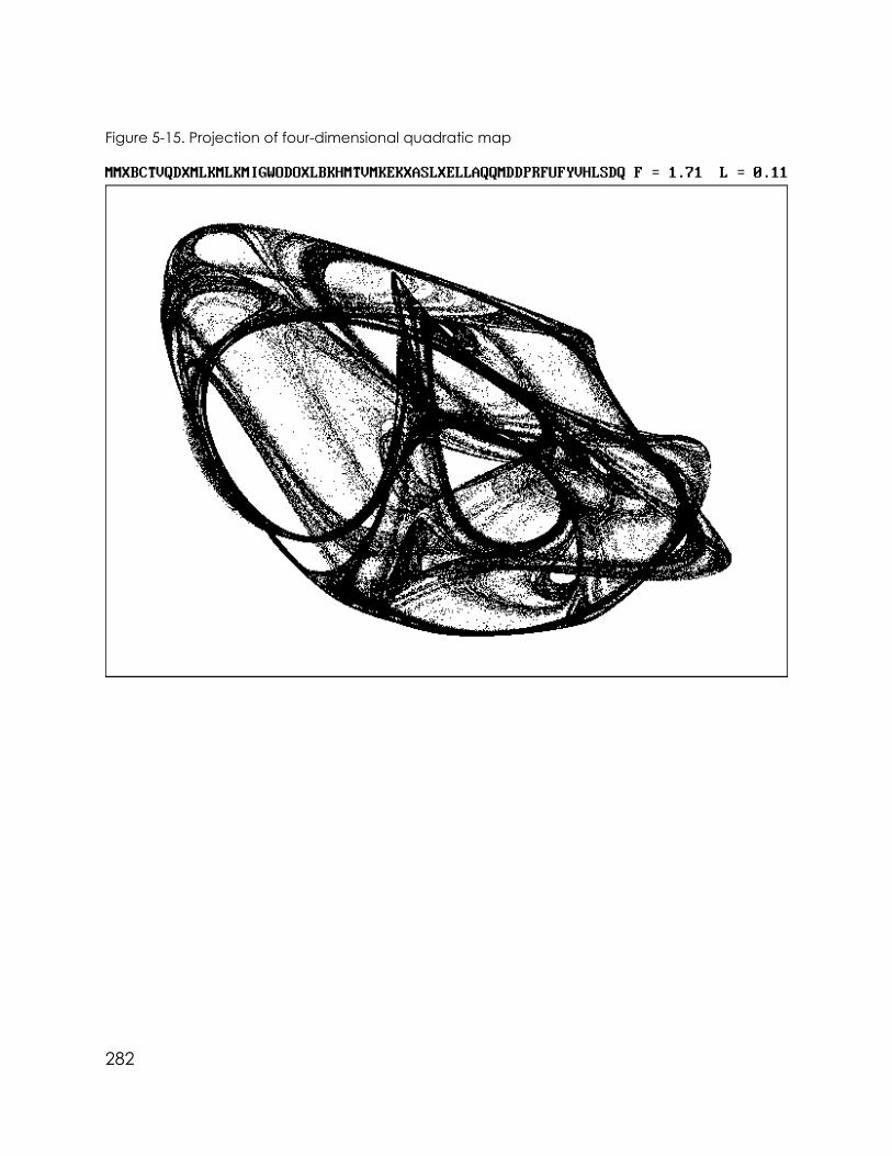
Figure 5-15. Projection of four-dimensional quadratic map
282

Figure 5-16. Projection of four-dimensional quadratic map
283

Figure 5-17. Projection of four-dimensional quadratic map
284

Figure 5-18. Projection of four-dimensional cubic map
285

Figure 5-19. Projection of four-dimensional cubic map
286
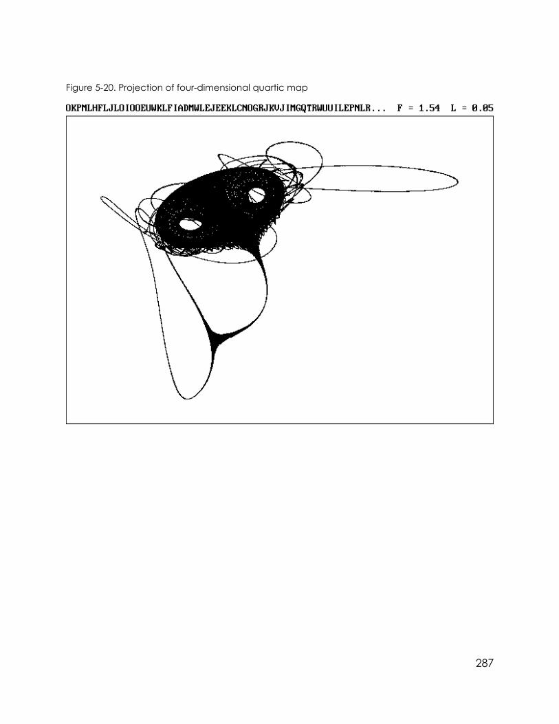
Figure 5-20. Projection of four-dimensional quartic map
287
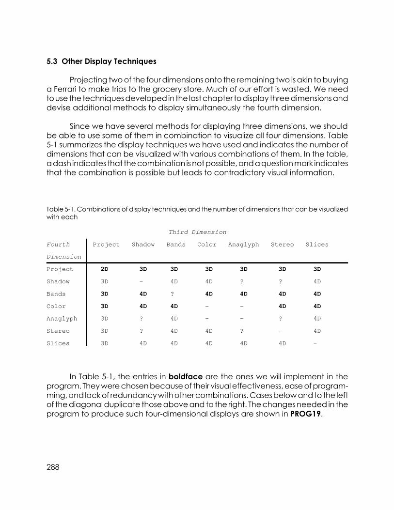
5.3 Other Display Techniques
Projecting two of the four dimensions onto the remaining two is akin to buyinga Ferrari to make trips to the grocery store. Much of our effort is wasted. We needto use the techniques developed in the last chapter to display three dimensions anddevise additional methods to display simultaneously the fourth dimension.
Since we have several methods for displaying three dimensions, we shouldbe able to use some of them in combination to visualize all four dimensions. Table5-1 summarizes the display techniques we have used and indicates the number ofdimensions that can be visualized with various combinations of them. In the table,a dash indicates that the combination is not possible, and a question mark indicatesthat the combination is possible but leads to contradictory visual information.
Table 5-1. Combinations of display techniques and the number of dimensions that can be visualizedwith each
Third Dimension
Fourth Project Shadow Bands Color Anaglyph Stereo Slices
Dimension
Project 2D 3D 3D 3D 3D 3D 3D
Shadow 3D - 4D 4D ? ? 4D
Bands 3D 4D ? 4D 4D 4D 4D
Color 3D 4D 4D - - 4D 4D
Anaglyph 3D ? 4D - - ? 4D
Stereo 3D ? 4D 4D ? - 4D
Slices 3D 4D 4D 4D 4D 4D -
In Table 5-1, the entries in boldface are the ones we will implement in theprogram. They were chosen because of their visual effectiveness, ease of program-ming, and lack of redundancy with other combinations. Cases below and to the leftof the diagonal duplicate those above and to the right. The changes needed in theprogram to produce such four-dimensional displays are shown in PROG19.
288

PROG19. Changes required in PROG18 to display the fourth dimension
1000 REM FOUR-D MAP SEARCH (With 4-D Display Modes)
1040 PREV% = 5 'Plot versus fifth previous iterate
1120 TRD% = 1 'Display third dimension as shadow
1130 FTH% = 2 'Display fourth dimension as colors
3630 IF Q$ = "" OR INSTR("ADHIPRSX", Q$) = 0 THEN GOSUB 4200
3720 IF Q$ = "H" THEN FTH% = (FTH% + 1) MOD 3: T% = 3: IF N > 999 THEN N = 999:GOSUB 5600
4330 PRINT TAB(27); "H: Fourth dimension is ";
4340 IF FTH% = 0 THEN PRINT "projection"
4350 IF FTH% = 1 THEN PRINT "bands "
4360 IF FTH% = 2 THEN PRINT "colors "
5010 C4% = WH%
5020 IF D% < 4 THEN GOTO 5050
5030 IF FTH% = 1 THEN IF INT(30 * (W - WMIN) / (WMAX - WMIN)) MOD 2 THEN GOTO5330
5040 IF FTH% = 2 THEN C4% = 1 + INT(NC% * (W - WMIN) / (WMAX - WMIN) + NC%)MOD NC%
5050 IF D% < 3 THEN PSET (XP, YP): GOTO 5330 'Skip 3-D stuff
5060 IF TRD% = 0 THEN PSET (XP, YP), C4%
5080 IF D% > 3 AND FTH% = 2 THEN PSET (XP, YP), C4%: GOTO 5110
5130 IF TRD% <> 2 THEN GOTO 5160
289

5140 IF D% > 3 AND FTH% = 2 AND (INT(15 * (Z - ZMIN) / (ZMAX - ZMIN) + 2) MOD2) = 1 THEN PSET (XP, YP), C4%
5150 IF D% < 4 OR FTH% <> 2 THEN C% = COLR%(INT(60 * (Z - ZMIN) / (ZMAX - ZMIN)+ 4) MOD 4): PSET (XP, YP), C%
5260 XRT = XA + (XP + XZ * (Z - ZA) - XL) / HSF: PSET (XRT, YP), C4%
5270 XLT = XA + (XP - XZ * (Z - ZA) - XH) / HSF: PSET (XLT, YP), C4%
5320 PSET (XP, YP), C4%
5630 IF TRD% = 3 OR (D% > 3 AND FTH% = 2 AND TRD% <> 1) THEN FOR I% = 0 TO NC%:COLR%(I%) = I% + 1: NEXT I%
In presenting sample displays from PROG19, we ignore those that conveyonly three-dimensional information and concentrate on the new combinationsthat permit full four-dimensional displays. They fall into two groups—those thatrequire the use of color and those that do not. Examples of the three 4-D mono-chrome combinations are shown in Figures 5-21 through 5-44, and examples of thesix color combinations are shown in Plates 17 through 22.
290

Figure 5-21. Four-dimensional quadratic map with shadow bands
291

Figure 5-22. Four-dimensional quadratic map with shadow bands
292

Figure 5-23. Four-dimensional quadratic map with shadow bands
293

Figure 5-24. Four-dimensional quadratic map with shadow bands
294

Figure 5-25. Four-dimensional quadratic map with shadow bands
295

Figure 5-26. Four-dimensional quadratic map with shadow bands
296

Figure 5-27. Four-dimensional quadratic map with shadow bands
297
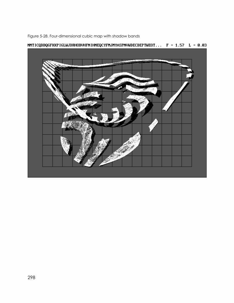
Figure 5-28. Four-dimensional cubic map with shadow bands
298

Figure 5-29. Four-dimensional quadratic map with stereo bands
299
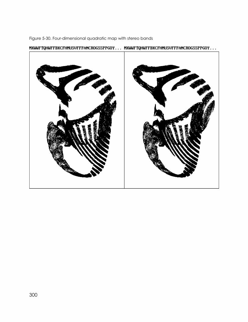
Figure 5-30. Four-dimensional quadratic map with stereo bands
300

Figure 5-31. Four-dimensional quadratic map with stereo bands
301

Figure 5-32. Four-dimensional cubic map with stereo bands
302

Figure 5-33. Four-dimensional cubic map with stereo bands
303

Figure 5-34. Four-dimensional cubic map with stereo bands
304

Figure 5-35. Four-dimensional quartic map with stereo bands
305

Figure 5-36. Four-dimensional quartic map with stereo bands
306

Figure 5-37. Four-dimensional quadratic map with sliced bands
307

Figure 5-38. Four-dimensional quadratic map with sliced bands
308

Figure 5-39. Four-dimensional quadratic map with sliced bands
309
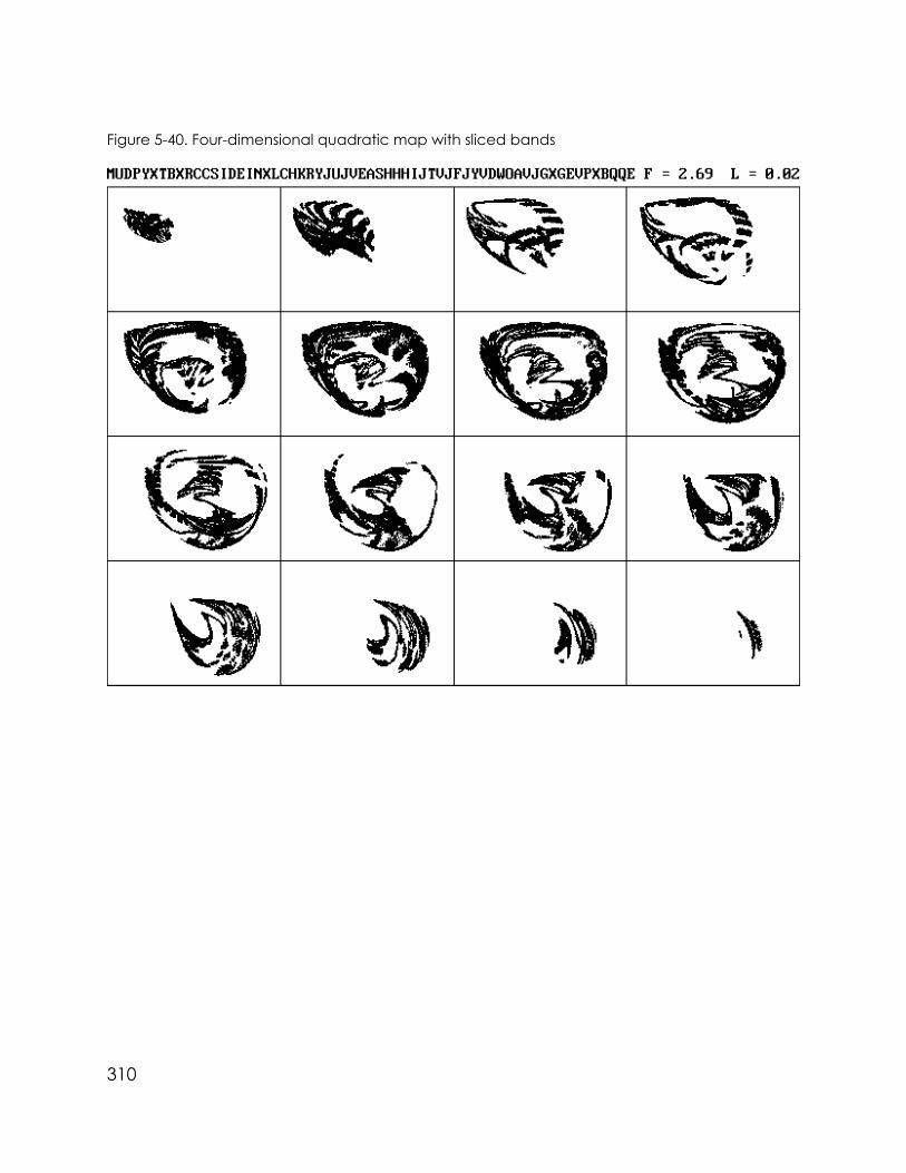
Figure 5-40. Four-dimensional quadratic map with sliced bands
310

Figure 5-41. Four-dimensional cubic map with sliced bands
311

Figure 5-42. Four-dimensional quartic map with sliced bands
312

Figure 5-43. Four-dimensional quartic map with sliced bands
313

Figure 5-44. Four-dimensional quintic map with sliced bands
You might be interested in the challenge of producing attractors embeddedin dimensions higher than four. In five dimensions, you need to define a newvariable, say V, and modify the program as was done for four dimensions in PROG18.The program has been written to make it relatively easy to extend it to five or evenhigher dimensions. Be forewarned that the calculation will be very slow. You willalmost certainly want to set the coefficients of the constant terms to zero andprobably restrict your search to quadratic maps. The number of fifth-dimensionpolynomial coefficients for order O is (O + 1)(O + 2)(O + 3)(O + 4)(O + 5) / 24. WithO = 5, the number is 1260.
The simplest display technique is to project the fifth dimension onto the otherfour. This is what the program does automatically if you don’t do anything special.Several combinations of techniques, which we have already developed, arecapable of displaying five dimensions. You might try combining shadows, bands,
314

and color, for example. Table 5-2 lists the seven possible combinations of five-dimensional display techniques that don’t lead to visual contradictions.
Table 5-2. Combinations of display techniques that can be used in five dimensions
Shadow Bands Color
Shadow Bands Slices
Shadow Color Slices
Bands Color Stereo
Bands Anaglyph Slices
Bands Stereo Slices
Color Stereo Slices
For a heroic exercise in programming, visualization, and patience, you cantry to extend the calculation to six dimensions. A six-dimensional, fifth-order systemof polynomials has 2772 coefficients. There are only two appropriate combinationsof display techniques suitable for six dimensions: shadow-bands-color-slices andbands-color-stereo-slices. If you decide to try seven dimensions, you must invent anew display technique.
5.4 Writing on the Wall
Since four-dimensional attractors have the greatest complexity and varietyof all the cases described in this book, they offer the greatest potential as displayart. For such purposes, you will probably want to print them on a large sheet ofpaper. With an appropriate printer or plotter, any of the visualization techniquespreviously described can be used to produce such large prints.
An alternate technique that has proved very successful is an extension of thecharacter-based method described in Section 4.5. In this technique, the thirddimension is coded as an ASCII character with a density related to the Z value, andthe fourth dimension is coded in color. Color pen and pencil plotters and ink-jetplotters, as well as more expensive but high-quality electrostatic and thermalplotters, normally used for engineering and architectural drawings, can print text onsheets up to 36 inches wide. Ink-jet plotters are growing in popularity over the more
315

traditional pen plotters because they are faster and quieter and don’t requirespecial paper. They can also print gray scales. With care, you can piece togethersmaller segments printed by more conventional means.
When the attractors are reduced to sequences of text, resolutions of 640 by480 (VGA) or 800 by 600 (Super VGA) produce large figures whose individualcharacters can be read when examined closely but that blend into continuouscontours when viewed from a distance. Artists often use this technique in which theviewer is provided with a different visual experience on different scales. You shoulduse the largest and boldest characters available to maximize the contrast, pro-vided they remain readable. There should be little or no space between rows andcolumns of characters. With a pen plotter, the pen size can be chosen for the bestcompromise of contrast and readability. A pen that makes a line width of 0.35 mm(fine) is a reasonable choice.
Inks are available in only a limited number of colors, and pen plotters areusually capable of accommodating only a small number of pens. The pens can besequenced to place compatible colors next to one another. With eight pens andcommonly available inks, a good sequence is magenta, red, orange (or yellow),brown, black, green, turquoise, and blue. The closest color sequence for viewing onthe computer screen from Table 4-1 is 13, 12, 4 (or 14), 6, 8, 2, 3, and 9, with a white(15) background. With upwards of 20 characters producing different color intensi-ties, the limitation of eight colors of ink is not a serious one. With eight colors and ASCIIcodes from 32 to 255, you can have 28 different intensities for each color. The inkscan be mixed to produce different shades of the colors. Pencils are less expensiveand don’t clog or dry out as pens often do, but pencil plots have a tendency tosmudge. Ink, of course, also smudges until it is thoroughly dry. Plotters are relativelyslow, and attractors produced by this method typically require a few hours to a fullday to produce.
Paper commonly used for engineering drawings comes in at least fivestandard sizes—A (8 1/2 by 11 inches), B (12 by 18 inches), C (18 by 24 inches), D (24by 36 inches), and E (36 by 48 inches). English sizes and architectural sizes are slightlydifferent, and thus a sheet may vary somewhat from these dimensions. Also, 36-inch-wide paper is available on long rolls.
Common paper types are tracing bond, which is the most economical,vellum, which is smooth and translucent, and polyester film, which is highly translu-cent, dimensionally stable, and relatively expensive. The translucent papers offerthe interesting possibility of backing the print with a monochrome or color copy ofitself to enhance the contrast or to produce a shadow effect if the two aredisplaced slightly. Other interesting effects can be achieved by backing one
316

translucent attractor with a print of another or by back-lighting the print. Somepapers stretch slightly and thus have a tendency to wrinkle. Paper with significantacid content should be avoided because it turns yellow and becomes brittle withage.
Some of the most artistic examples of strange attractors have been pro-duced by these techniques, but they cannot be adequately illustrated in this book.No computer program is offered, since it is so dependent on your hardware. You willwant to experiment to find the technique that works best for you and that makesthe most effective use of your printer or plotter.
5.5 Murals and Movies
The technique of making large-scale attractors for display can be carried toits logical extreme by making a mural. Special techniques using some type of stencilare required to transform the computer output to paint on the wall. Silk screen isuseful for transferring the image to fabrics. Fractal tee-shirts employing this tech-nique have recently become popular.
To produce a mural, you need to start with a large number of plots, eachshowing a small section of the attractor. A property of fractals is that they havedetail on all scales, and thus a large mural should look interesting when viewedeither from a distance or close up.
You might also photograph the computer screen or a high-quality print andproduce slides that can be projected onto a large surface or screen with a slideprojector. Equipment is available commercially for producing slides directly fromdigital computer output. A sequence of such slides makes a very compellingpresentation or visual accompaniment to a lecture or musical production.
The color slices shown in Plate 22 suggest the possibility of making colormovies by extending the technique to a very large number of slices and using eachone as a frame of a movie. The effect is to cause the attractor to emerge at a pointin an empty field and to grow slowly, bending and wiggling until fully developed,and then to disappear slowly into a different point. If the technology for doing thisis not available to you, try printing a large number of attractor slices on small cardsand fanning through them to produce a semblance of animation. This technique,using the attractors described in Section 7.6, was used to produce the animationin the upper-right corner of the odd pages of this book.
317

If the idea of making strange-attractor movies appeals to you, anothertechnique is to take one of your favorite attractors and slowly change one or moreof the coefficients in successive frames of the movie. A good way to start is tomultiply all the coefficients by a factor that varies from slightly less than 1.0 to slightlygreater than 1.0. You must determine the range over which the coefficients can bechanged without the solutions becoming unbounded or nonchaotic. The ends ofthis range then become the beginning and end of the movie.
Sometimes the attractor slowly and continuously alters its shape. The changescan involve bifurcations, such as the period-doubling sequence in the logisticequation described in Chapter 1. Such bifurcations are called subtle. At other times,the attractor and its basin abruptly disappear at a critical value of the controlparameter. Such discontinuous bifurcations are called catastrophes.
If the control parameter is changed in the opposite direction, the result maybe different from simply running the movie backward. This is an example ofhysteresis, which is a form of memory in a dynamical system. It serves to limit theoccurrence of catastrophes. The thermostat that controls your heat probably useshysteresis to keep the furnace from cycling on and off too frequently. Catastrophicbifurcations usually exhibit hysteresis, whereas subtle bifurcations do not.
These four-dimensional maps are also well suited for color holographicdisplay or for experimentation with virtual reality, in which the view is controlled bythe motion of your head and hands to give the sensation of moving through theobject. The technology is complicated, but the results are visually and mentallystimulating.
5.6 Search and Destroy
If you have worked carefully through the text, your program has created adisk file SA.DIC containing the codes of all the attractors generated since you ranthe PROG11 program. We now develop the capability to examine these attractorsand save the interesting ones in a file FAVORITE.DIC, while discarding the others. Thisfeature allows you to run the program overnight and collect attractors for rapidviewing the next day. This capability is especially useful if you have a slow computer.The required program changes are shown in PROG20.
PROG20. Changes required in PROG19 to evaluate the attractors in SA.DIC and save the best of
318

them in FAVORITE.DIC
1000 REM FOUR-D MAP SEARCH (With Search and Destroy)
1380 IF QM% <> 2 THEN GOTO 1420
1390 NE = 0: CLOSE
1400 OPEN "SA.DIC" FOR APPEND AS #1: CLOSE
1410 OPEN "SA.DIC" FOR INPUT AS #1
2420 IF QM% = 2 THEN GOTO 2490 'Speed up evaluation mode
2610 IF QM% <> 2 THEN GOTO 2640 'Not in evaluate mode
2620 IF EOF(1) THEN QM% = 0: GOSUB 6000: GOTO 2640
2630 IF EOF(1) = 0 THEN LINE INPUT #1, CODE$: GOSUB 4700: GOSUB 5600
3340 IF QM% <> 2 THEN GOTO 3400 'Not in evaluate mode
3350 LOCATE 1, 1: PRINT "<Space Bar>: Discard <Enter>: Save";
3370 LOCATE 1, 49: PRINT "<Esc>: Exit";
3380 LOCATE 1, 69: PRINT CINT((LOF(1) - 128 * LOC(1)) / 1024); "K left";
3390 GOTO 3430
3620 IF QM% = 2 THEN GOSUB 5800 'Process evaluation command
3630 IF INSTR("ADEHIPRSX", Q$) = 0 THEN GOSUB 4200
3710 IF Q$ = "E" THEN T% = 1: QM% = 2
319

4220 WHILE Q$ = "" OR INSTR("AEIX", Q$) = 0
4320 PRINT TAB(27); "E: Evaluate attractors"
5800 REM Process evaluation command
5810 IF Q$ = " " THEN T% = 2: NE = NE + 1: CLS
5820 IF Q$ = CHR$(13) THEN T% = 2: NE = NE + 1: CLS : GOSUB 5900
5830 IF Q$ = CHR$(27) THEN CLS : GOSUB 6000: Q$ = " ": QM% = 0: GOTO 5850
5840 IF Q$ <> CHR$(27) AND INSTR("HPRS", Q$) = 0 THEN Q$ = ""
5850 RETURN
5900 REM Save favorite attractors to disk file FAVORITE.DIC
5910 OPEN "FAVORITE.DIC" FOR APPEND AS #2
5920 PRINT #2, CODE$
5930 CLOSE #2
5940 RETURN
6000 REM Update SA.DIC file
6010 LOCATE 11, 9: PRINT "Evaluation complete"
6020 LOCATE 12, 8: PRINT NE; "cases evaluated"
6030 OPEN "SATEMP.DIC" FOR OUTPUT AS #2
6040 IF QM% = 2 THEN PRINT #2, CODE$
6050 WHILE NOT EOF(1): LINE INPUT #1, CODE$: PRINT #2, CODE$: WEND
320

6060 CLOSE
6070 KILL "SA.DIC"
6080 NAME "SATEMP.DIC" AS "SA.DIC"
6090 RETURN
The program uses the E key to enter the evaluation mode. When in this mode,the attractors in SA.DIC are displayed one by one. Each case remains on the screenand continues to iterate until you press the spacebar, which deletes it, the Enter key,which saves it in the file FAVORITE.DIC, the Esc key, which exits the evaluation mode,or, in rare cases, until the solution becomes unbounded, whereupon it is deleted.While an attractor is being displayed, you can press the H, R, P, and S keys to changethe way it is displayed without returning to the menu screen. The upper-right cornerof the screen shows the number of kilobytes left to be evaluated in the SA.DIC file.When in the evaluation mode, the program bypasses the calculation of the fractaldimension and Lyapunov exponent so that each case is displayed more quickly.
As you begin to accumulate a collection of favorite attractors, you willprobably want to go back and find your favorites of the favorites. You merely needto rename the FAVORITE.DIC file to SA.DIC and evaluate them a second time. Theattractors exhibited in this book were selected by this method after looking at about100,000 cases. Since the FAVORITE.DIC file is in ordinary ASCII text, you can shareyour favorites with a friend who may have a different computer or operating system.You can easily e-mail the file to someone or upload it to a computer bulletin boardor mainframe computer. Remember, however, that the programs in this book arecopyrighted and are for your personal use. It is a violation of the copyright to sharethe programs with anyone else. You can now begin your own private collection ofstrange attractors artwork!
321

Chapter 6Fields and Flows
In this chapter, we consider equations whose iterates move gradually ratherthan abruptly from one place to another. Such equations are called differentialequations, and they are the basis for most dynamical systems that describe naturalprocesses. The programming is a simple extension of what we have done before,but the calculation requires more computing time. The attractors produced bydifferential equations consist of continuous lines whose weavings and waveringsdescribe the trajectory and yield objects of considerable beauty.
6.1 Beam Me Up Scotty!
Successive iterates of the maps in the previous chapters are usually at widelydifferent positions on the attractors. The points dance around like fleas jumping onthe back of a dog, eventually, but gradually, visiting every allowed location. Mostprocesses in nature don’t occur that way but progress slowly and continuously fromsome initial condition through a succession of nearby intermediate states to thefinal condition.
If you take a trip across the country, your trajectory through three-dimen-sional space (or even in four-dimensional space-time) is a continuous one-dimen-sional curve. Only in science fiction is Captain Kirk able to dematerialize at oneposition and rematerialize somewhere else, without occupying a succession ofintermediate positions. Most substances in nature obey a continuity equation,which guarantees that if their quantity decreases at some position, the decreasemust be accompanied by a flow of the substance away from the position. Note thatthis is a stronger condition than a conservation law, which requires only that the totalquantity of the substance remains the same.
There is a relation between flows and maps. Imagine a fly trapped in a roomand moving in a complicated, random manner. Its trajectory is a one-dimensionalcurve that eventually fills the entire room. However, if you observe the fly with astrobe lamp that flashes periodically, the trajectory is a succession of dots, witheach dot separated from the previous dot by a significant distance. The dots alsoeventually fill the entire three-dimensional region, but it takes longer for this to occur.
However, if the fly’s motion is chaotic rather than random, neither the curve
322

nor the dots fill the room; rather, they lie on a strange attractor that occupies anegligible portion of the room. The attractor consisting of all the possible dots oftenhas a lower dimension than the attractor consisting of all the possible curves. Thusa map can be thought of as a crude description of a flow, in which the interveningdetails of the motion are ignored.
It’s easy to think of an object such as a fly or a human, imbued withintelligence, however limited, moving by free will along a complicated trajectory.However, inanimate objects, such as astronomical bodies or sub-microscopic,electrically charged particles, can also execute complicated motions. They do sobecause they move through a space filled with gravitational or electromagneticfields.
It is important to recognize that a field has no objective reality other than todescribe mathematically the force on an object moving through it. When some-thing is dropped, it falls toward Earth. It is a deeply philosophical question, notanswered very well by science, how the object knows to move toward Earth ratherthan in some other direction. We say that it is acted upon by the gravitational fieldof the Earth, but this description, however useful for calculating the motion, begs theissue. Ultimately, the laws of physics describe very accurately how things move, butnot very well why.
The equations that describe flows are of a different type than those thatdescribe maps. They are called differential equations, and they involve the rate ofchange of a quantity. We will consider only ordinary differential equations (ODEs),as distinguished from the partial differential equations (PDEs) used to describe thebehavior of complicated objects like fluids that have intrinsically infinite-dimen-sional state spaces. Dynamical systems described by ODEs involve only the timerate of change of the position of a point in state space, whereas with PDEs, thevariables are quantities like density, temperature, and electric field that change inspace as well as time. A wave is an example of a dynamical system described bya PDE.
Consider an object moving in the X direction. Its speed is the rate of changeof its position, and we will denote this quantity by X’ (pronounced "X prime"). It is thedistance the object moves in a brief interval of time divided by the time interval. Ifyou know some calculus, you recognize this as the time-derivative of X, usuallydenoted by dX/dt. The rate of change of position is what the speedometer on yourcar, or the police radar, reads. The rate of change of the speed is the acceleration.More properly, we should call these quantities the time rate of change, sincequantities can also change in space. For example, the spatial rate of change inaltitude of a road is called its grade.
323

An object moving in three-dimensional space has a constantly changingvalue not only of X but also of Y and Z. Furthermore, X’, Y’, and Z’ usually dependon position (X, Y, and Z). For example, a particle moving clockwise in a circle aboutthe origin in the XY plane is described by the following pair of differential equations:
X’ = Y
Y’ = -X (Equation 6A)
Such a set of equations describes, at least approximately, the motion of the eartharound the sun. This type of regular motion is not chaotic, and it does not lead tovisually interesting strange attractors.
Some differential equations can be solved easily using calculus. For example,Equation 6A has the solution
X = A sin(t + _)
Y = A cos(t + _) (Equation 6B)
which specifies the X and Y positions at any time t. The quantities A and φ areconstants that are determined from the initial conditions (the values of X and Y att = 0). If you are interested only in the shape of the trajectory, and not in where theobject is along it at any particular time, you can eliminate the t in Equations 6B toget a relation between X and Y,
X2 + Y2 = A2 (Equation 6C)
which is the equation for a circle of radius A centered on the origin (X = Y = 0).
Equation 6A also arises in a different context. Imagine an object moving backand forth in the X direction, perhaps attached to a spring that alternately stretchesand compresses. Since Y is equal to X’, we can associate Y with the velocity in theX direction. The XY plane then becomes the two-dimensional phase space for thisone-dimensional motion, and the trajectory in this plane is the phase-spacetrajectory. A circular phase-space trajectory is a characteristic of a one-dimen-sional, simple harmonic oscillator, such as a mass on a spring. Usually the phase-space trajectory is an ellipse, just as the orbit of the earth around the sun is an ellipse,but we can always measure Y in appropriate units, or adjust the scale of the graph,to change the ellipse into a circle.
With this interpretation, the first part of Equation 6A defines the velocity (Y) as
324

the rate of change of position (X’). If you remember your physics, the second partof Equation 6A is Newton’s second law (F = ma), in which the force F obeys Hooke’slaw for springs (F = - kX), and the acceleration a is the rate of change of velocity (Y’).It is interesting that the same set of differential equations with a change in themeaning of the variables can describe the motion of an object traveling in a circleor an object oscillating on the end of a spring. Equation 6A describes many otherphenomena in nature, such as the oscillations in an electrical circuit containing acapacitor and inductor.
A two-dimensional system of differential equations such as Equation 6Acannot exhibit chaos, according to the Poincaré-Bendixon theorem, because thetrajectory cannot cross itself. The most complicated bounded behavior is thus asimple closed loop, corresponding to periodic motion. The reason the trajectorycannot cross itself is that every point in the XY plane has associated with it a uniquedirection of flow, so the trajectory must approach and leave every point in a singleparticular direction. If the orbit were to return to a point previously visited, it wouldthereafter repeat what it did before. In two dimensions, the orbit can do only oneof three things: spiral into a fixed point, approach a stable limit cycle, or spiral off toinfinity.
Trajectories may appear to cross if they come very close to a fixed point thatis stable in one direction and unstable in another (called a saddle point or X pointbecause of its shape). Such a trajectory is called a separatrix because it separatesregions with different flows. Trajectories approaching the fixed point on one side ofthe separatrix veer off to the right, and those approaching from the other side veeroff to the left. Such a separatrix exists upstream (and downstream) of an island in ariver where two sticks placed side by side in the water end up going aroundopposite sides of the island. The island seems at first to attract the sticks and then torepel them at right angles as they approach it.
In three dimensions, we have the possibility of an orbit wrapping around in acomplicated manner, like a ball of string, never intersecting itself, but producing anever-ending tangle. By contrast, maps can be chaotic in one or two dimensionsbecause the points jump from place to place with little danger of intersectinganother point. Captain Kirk need not be concerned about a collision while beingtransported from one point to another. He only needs to worry about landing on topof a diabolical Romulan at his destination!
325

6.2 Professor Lorenz and Dr. Rössler
Although differential equations have been the mathematical basis for mostdescriptions of nature for hundreds of years, almost no one suspected that thetrajectories resulting from their solution could be a chaotic strange attractor. Thehistory of the discovery of such solutions is interesting and bears retelling.
In the early 1960s, Edward Lorenz, a meteorologist at the MassachusettsInstitute of Technology, was developing models of atmospheric convection to besolved by a primitive computer that required about one second per iteration. Hismodels involved a large number of differential equations and produced solutionsthat varied with time in a complicated manner, not unlike the variation of theweather over long intervals of time. On one occasion, he happened to restart oneof his computer runs using numbers rounded to three digits rather than the sixsignificant figures used by the computer.
For some time, the solutions followed one another, but after a while theybegan to depart, and eventually they bore no relation to one another. He haddiscovered the sensitivity to initial conditions that is perhaps the most salient featureof chaos. He began simplifying his equations in an attempt to determine theminimum conditions necessary for this bizarre behavior. The result is the now famousLorenz equations, which represent the first example of a strange attractor arisingfrom differential equations,
X’ = _(Y - X)
Y’ = -XZ + rX - Y
Z’ = XY - bZ (Equation 6D)
where σ, r, and b are constants that Lorenz took to be σ = 10, r = 28, and b = 8/3.Lorenz published his findings in 1963 in the Journal of the Atmospheric Sciences,where they went largely unnoticed for the next decade. The title of his paper,"Deterministic Nonperiodic Flow," is an apt description of what we now call chaos.
Although the Lorenz equations were distilled from a model of atmosphericconvection, the trajectory in XYZ space does not represent air currents in any literalway. Instead, X corresponds to the size of the convective motion, Y is proportionalto the temperature difference between the ascending and descending fluids, andZ is proportional to the deviation of the vertical temperature profile from a linearfunction. Nevertheless, the behavior is reminiscent of a fluid with turbulent convec-tion.
326

Since the Lorenz equations were proposed, several phenomena have beenfound that are at least approximately modeled by them. Perhaps the simplestexample is the thermosiphon. Imagine a continuous tube, like a bicycle tube, filledwith a liquid and mounted vertically. If the bottom of the tube is heated and the topcooled, a convection ensues, with the warm fluid rising and the cold fluid falling. Theconvection is equally likely to start in either direction. After it starts, the circulationcontinues in that direction a few times around the loop and then abruptly reverses.
In the 1970s other examples of chaotic differential equations began to bediscovered. An important contribution was made in 1976 by Otto Rössler, anonpracticing medical doctor in Germany. Rössler was interested in chaos inchemistry and theoretical biology, and he set about to find a system of equationseven simpler than those of Lorenz that exhibited chaotic behavior. What he cameup with are the now famous Rössler equations:
X’ = -(Y + Z)
Y’ = X + aY
Z’ = b + Z(X - c) (Equation 6E)
where a, b, and c are constants that Rössler took to be a = 0.2, b = 0.2, and c = 5.7.The Rössler equations are sometimes described as the simplest known example ofchaos arising from a system of ordinary differential equations. They contain a singlenonlinearity (ZX in the third equation). Rössler’s original paper is also interestingbecause it contains a stereoscopic view of his strange attractor as well as the Lorenzattractor.
Until very recently, the discovery of a new strange attractor was a cause torush to publication. With the program in this book, you can produce them by thethousands! Even today researchers tend to focus on a few well-known examplessuch as the Lorenz and Rössler attractors. An entire book has been written on theLorenz attractor alone. Think of the libraries that could be filled by books describingyour attractors in similar detail!
The Lorenz and Rössler attractors are shown in Figures 6-1 and 6-2, respec-tively, albeit with slightly different values of the parameters than they used. Thesecases are known to have fractal dimensions slightly greater than 2.0. Theseexamples are more important for their historical interest than for their visual appeal.If you have never seen these attractors in 3-D, be sure to return to these cases andview them with the various display techniques after the program has been appro-priately modified, as described in the next section. The Lorenz attractor resembles
327

the wings of a butterfly, making it an appropriate emblem of chaos, since thesensitivity to initial conditions is most dramatically illustrated by the butterfly effect.
Figure 6-1. The Lorenz attractor
328

Figure 6-2. The Rössler attractor
6.3 Finite Differences
Some differential equations, such as Equation 6A, can be solved exactly in astraightforward manner using calculus. However, if a system of equations exhibitschaos, no such solution is possible. The reason is that no mathematical functionanalogous to the sine and cosine can describe a strange attractor the way thosefunctions describe a circle. The equations must be solved by computer. We say thatsuch solutions are numerical as opposed to analytical.
Unfortunately, digital computers, which are ideal for iterating maps, areinherently incapable of exactly solving differential equations. The equations requirethat the solution advance slowly and smoothly. That is, the successive iterates mustdiffer by an infinitesimal amount, thus infinitely many iterations are required to makeany progress. Special analog computers have been designed for the task, but they
329

are not common or simple to program.
Books have been written on methods for the approximate numerical solutionof differential equations, and it is as much an art as a science. All the methodsinvolve, in one form or another, a finite-difference approximation to the differentialequation. Rather than taking infinitesimal steps, one advances in finite stepsaccording to a prescription that attempts to minimize the inevitable errors. Fortu-nately, for our purpose, our solutions need not be highly accurate, so we can usea simple procedure.
Perhaps the easiest and most transparent method for finding approximatesolutions to differential equations is the Euler method. When this procedure isapplied to the simple example of Equation 6A, X and Y are advanced accordingto
Xn+1 = Xn + _Yn
Yn+1 = Yn - _Xn (Equation 6F)
where ε is the time step that ideally should be negligibly small but in reality is madeas large as possible to reduce the number of iterations required to advance thesolution by a substantial distance along the trajectory. You see that the Eulermethod provides just another example of an iterated map in which successiveiterates are near one another. It is perhaps the least accurate method for solvingdifferential equations, and it is easily improved upon. However, for most of ourpurposes, the Euler method is adequate. Furthermore, it is simple to modify theprogram to solve differential equations by this method. The necessary changes areshown in PROG21.
PROG21. Changes required in PROG20 to solve differential equations by the Euler method
1000 REM ODE SEARCH
1070 D% = 3 'Dimension of system
1080 EPS = .1 'Step size for ODE
1090 ODE% = 1 'System is ODE
330

1990 IF ODE% = 1 THEN XN(I%) = XY(I%) + EPS * XN(I%)
2660 CODE$ = CHR$(59 + 4 * D% + O% + 8 * ODE%)
3050 IF ODE% = 1 THEN L = L / EPS
3660 IF ODE% = 1 THEN D% = D% + 2
3680 IF Q$ = "D" THEN D% = 1 + (D% MOD 6): T% = 1
3700 IF D% > 4 THEN ODE% = 1: D% = D% - 2 ELSE ODE% = 0
4300 PRINT TAB(27); "D: System is"; STR$(D%); "-D polynomial ";
4310 IF ODE% = 1 THEN PRINT "ODE" ELSE PRINT "map"
4730 IF D% > 4 THEN D% = D% - 2: ODE% = 1 ELSE ODE% = 0
In PROG21, the value of ε is 0.1, and the three-dimensional equations arepolynomials up to fifth order, with coefficients chosen by analogy to the three-dimensional polynomial maps previously described. We don’t consider differentialequations in less than three dimensions because they cannot have chaoticsolutions. The second-order through fifth-order equations are coded with the firstletters Q, R, S, and T, respectively.
If ε is sufficiently small, its value should not affect whether a system is chaoticor the general appearance of the attractor, but it certainly changes the trajectoryon the attractor. Just as a chaotic trajectory is sensitive to initial conditions, it alsois sensitive to the approximations used to calculate it. Unfortunately, a value of ε =0.1 is not sufficiently small, and many of the resulting attractors would disappear orchange their appearance if ε were reduced. Conversely, other attractors wouldemerge for smaller values of e. Fortunately, for our purposes, the solutions need notbe even qualitatively correct. Be forewarned that reducing e has unpredictableeffects on the attractors and increases the computation time.
331

The Lyapunov exponent is calculated as with the corresponding maps,except that it is divided by e; thus its units are bits per second rather than bits periteration, because each iteration advances the solution by e seconds. It is custom-ary to express the Lyapunov exponent in this way for differential equations becausethe step size depends on the numerical approximation that is being used, whereasthe divergence of the trajectories per unit time is an intrinsic property of thedifferential equations.
Sample attractors produced by three-dimensional ordinary differential equa-tions projected onto the XY plane are shown in Figures 6-3 through 6-6.
Figure 6-3. Projection of three-dimensional quadratic ODE
332

Figure 6-4. Projection of three-dimensional cubic ODE
333

Figure 6-5. Projection of three-dimensional quartic ODE
334

Figure 6-6. Projection of three-dimensional quintic ODE
These figures are like time-exposed photographs of the shadow on the wallof a fly moving chaotically in a room. However, because of the finite differenceapproximation used to solve the equation of motion, you must imagine that the flyis illuminated by a strobe lamp that flashes rapidly. The trajectory thus consists of alarge number of closely spaced dots. The separation of the dots provides a measureof the accuracy of the solution. Although some of the cases produce apparentlycontinuous trajectories, others more nearly resemble the maps of the previouschapters. You might prefer to alter the program so that the dots are connected bylines. This is most easily done by changing line 5060 to
5060 IFTRD% = Ø THEN IFODE% = 1 THEN
LINE-(XP, YP), C4% ELSEPSET(XP, YP), C4%
Another consequence of dealing with differential equations is that many
335

criterion for the number of iterations as we did for the maps, a significant number(perhaps 20%) of the attractors found in a random search are not chaotic, and afew are even unbounded. When you evaluate the attractors found by the search,you will recognize these cases by the way they eventually settle onto a simpleclosed loop that is visually indistinguishable from a limit cycle, spiral into a fixed point,or leave the screen. You will also notice a few cases that consist of isolated islandswith no bridge connecting them, such as the one in Figure 6-3. You can be surethese are not true flows, because such discontinuities are impossible in the trajec-tories that arise from the solution of our differential equations.
There is no reason to limit the display of attractors arising from differentialequations to projections onto a plane. All the display techniques developed inChapter 4 for three-dimensional maps are also available here. Figures 6-7 through6-22 and Plates 23 and 24 show a selection of such examples.
Figure 6-7. Three-dimensional quadratic ODE with shadows
336

Figure 6-8. Three-dimensional cubic ODE with shadows
337

Figure 6-9. Three-dimensional quartic ODE with shadows
338

Figure 6-10. Three-dimensional quintic ODE with shadows
339
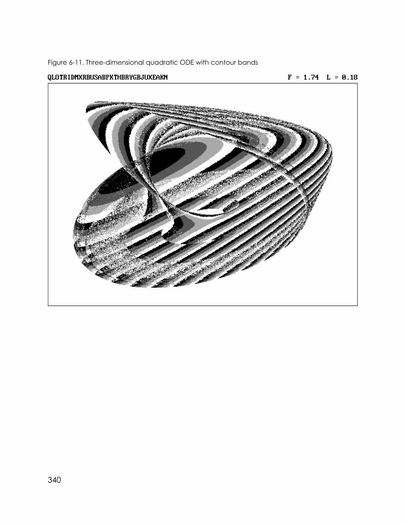
Figure 6-11. Three-dimensional quadratic ODE with contour bands
340

Figure 6-12. Three-dimensional cubic ODE with contour bands
341
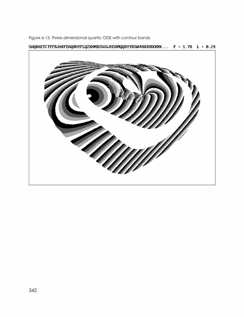
Figure 6-13. Three-dimensional quartic ODE with contour bands
342
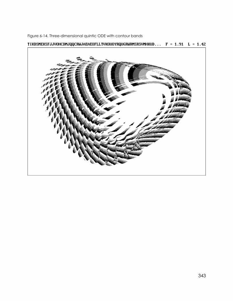
Figure 6-14. Three-dimensional quintic ODE with contour bands
343
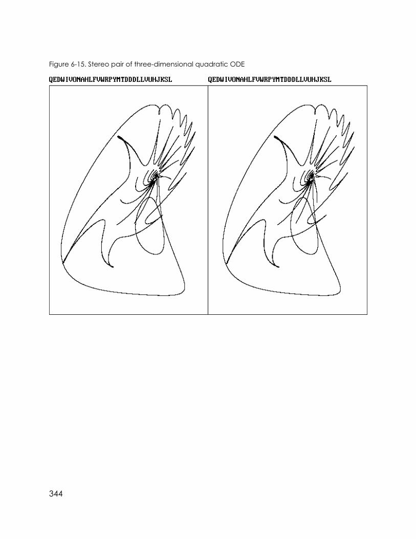
Figure 6-15. Stereo pair of three-dimensional quadratic ODE
344

Figure 6-16. Stereo pair of three-dimensional cubic ODE
345
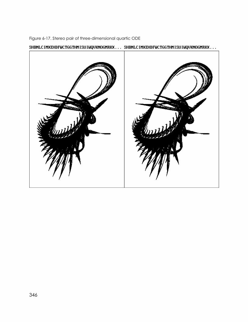
Figure 6-17. Stereo pair of three-dimensional quartic ODE
346
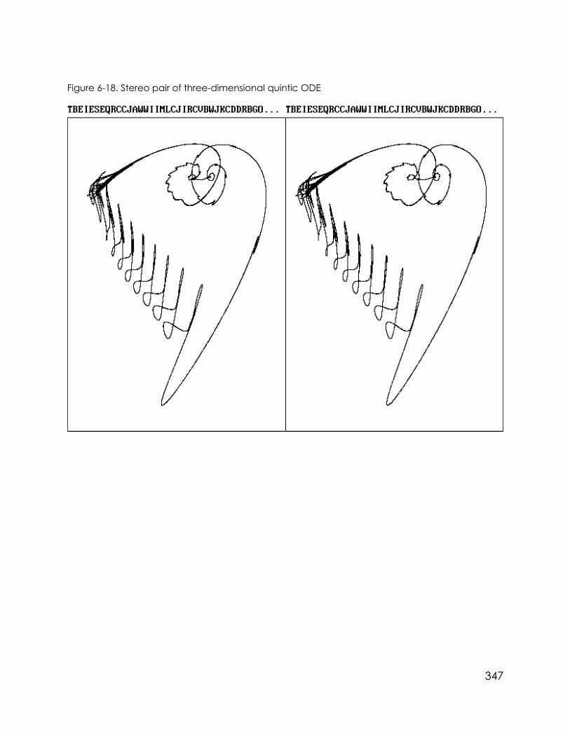
Figure 6-18. Stereo pair of three-dimensional quintic ODE
347

Figure 6-19. Slices of a three-dimensional quadratic ODE
348
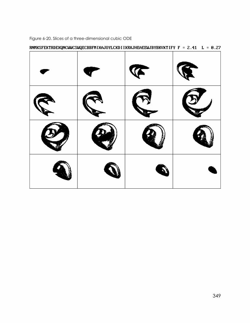
Figure 6-20. Slices of a three-dimensional cubic ODE
349

Figure 6-21. Slices of a three-dimensional quartic ODE
350

Figure 6-22. Slices of a three-dimensional quintic ODE
351

6.4 Flows in Four Dimensions
Flows, like maps, can be embedded in spaces of arbitrary dimension. Four-dimensional flows are hard to visualize but pose no difficulty for the computer tocalculate. Buried in PROG21 is the capability for calculating four-dimensional flows.You only need to press the D key to access the four-dimensional ODEs. All thetechniques previously developed for displaying four-dimensional maps are avail-able. The quadratic, cubic, quartic, and quintic equations are coded with the firstletters U, V, W, and X, respectively. Figures 6-23 through 6-38 and Plates 25 through30 show a selection of strange attractors arising from four-dimensional ordinarydifferential equations with polynomial terms.
Figure 6-23. Projection of a four-dimensional quadratic ODE
352

Figure 6-24. Projection of a four-dimensional cubic ODE
353
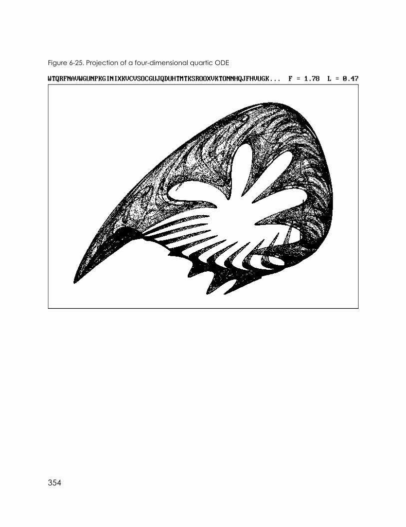
Figure 6-25. Projection of a four-dimensional quartic ODE
354

Figure 6-26. Projection of a four-dimensional quintic ODE
355

Figure 6-27. Four-dimensional quadratic ODE with shadow bands
356

Figure 6-28. Four-dimensional cubic ODE with shadow bands
357

Figure 6-29. Four-dimensional quartic ODE with shadow bands
358
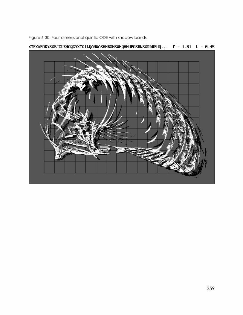
Figure 6-30. Four-dimensional quintic ODE with shadow bands
359

Figure 6-31. Four-dimensional quadratic ODE with stereo bands
360

Figure 6-32. Four-dimensional cubic ODE with stereo bands
361

Figure 6-33. Four-dimensional quartic ODE with stereo bands
362

Figure 6-34. Four-dimensional quintic ODE with stereo bands
363

Figure 6-35. Four-dimensional quadratic ODE with sliced bands
364

Figure 6-36. Four-dimensional cubic ODE with sliced bands
365

Figure 6-37. Four-dimensional quartic ODE with sliced bands
366

Figure 6-38. Four-dimensional quintic ODE with sliced bands
367

6.5 Strange Attractors that Aren’t
In Section 3.8, we discussed chaotic orbits that don’t approach an attractor("Strange Attractors that Don’t"). Here we consider nonchaotic orbits that ap-proach attractors that aren’t strange. These attractors are not fractals. They havedimensions that are integers such as 0, 1, 2, or 3. Some of them are beautiful, so theyare worth displaying even if they are technically outside the scope of this book.
Such attractors can arise from maps as well as from differential equations.They don’t require high embedding dimensions, although the dimension of theattractor always is at least one less than the dimension of the embedding space.Thus some of the examples are taken from equations described in earlier chapters.
The simplest nonchaotic attractor is a point attractor. Suppose we modifiedEquation 6A so the solution is not a circle but an inward spiral. One way to do thisis as follows:
X’ = Y - bX
Y’ = -X - bY (Equation 6G)
You can think of the coefficient b as a measure of the friction that eventually bringsthe trajectory to rest at the origin (X = Y = 0) in phase space. If b is zero (frictionless),the orbit is a circle. Negative values of b (antifriction) cause the solution to spiraloutward, approaching infinity. This case corresponds to a point repellor at theorigin. An attractive fixed point is called a sink and a repelling fixed point is calleda source. Some authors reserve the term fixed point for maps and prefer to call thestationary solutions of ODEs critical points or equilibrium points.
The two occurrences of b in Equation 6G need not have the same value oreven the same sign. In such a case, the orbit moves in or out but not in a symmetricalmanner. Many physical processes have b = 0 in one of the equations. If b is closeto zero, it doesn’t matter much in which equation it appears.
If b is zero in one of the equations above, small positive values of the other bcause the radius of the circle to decrease slowly, approaching what is called aspiral-point or focal-point attractor, or simply a focus. Larger positive values of bcause the radius to decrease more rapidly. With very large values of b, there is littlecirculation around the point, and the trajectory is more nearly radial toward whatis called a radial-point or nodal-point attractor, or simply a node. The boundarybetween the two cases occurs at b = 2 and corresponds to critical damping in anoscillator. In either case, the resulting attractor is a point at the origin with a
368

dimension of zero. A code that produces a point attractor (with b = 1) isQMLM3NM5LM3LM14. For this case, the largest Lyapunov exponent is negative (L= - 0.1/ln 2 = - 0.14), and it produces a single dot on the screen.
More interesting cases can occur because the program assumes the trajec-tory is on the attractor after 1000 iterations. For trajectories that approach theattractor very slowly, there can be interesting behavior after the thousandthiteration and before the fixed point is reached. Such slowly attracting fixed pointshave negative Lyapunov exponents, at least one of which is very close to zero. Thesearch can be expanded to include them as well as other nonchaotic attractorsby changing the .005 in line 2480 of the program to -.005, for example. Thenattractors that have Lyapunov exponents near zero but have not settled to a fixedpoint after NMAX iterations are included in the file SA.DIC. If you prefer, you cancollect them in a separate file TORUS.DIC by changing line 4910 of PROG21 to
4910 IF L > .005 THEN OPEN "SA.DIC" FOR APPEND AS #1 ELSE OPEN "TORUS.DIC" FOR
APPEND AS #1
Several such cases are shown in Figures 6-39 through 6-42. Figure 6-39 showsa spiral-point attractor. Figure 6-40 shows what appears to be a radial-pointattractor with several different initial conditions; it is really a spiral-point attractorwith successive iterates that move rapidly around the fixed point. This phenomenonis called aliasing, and it is most easily detected by connecting temporally succes-sive points with continuous lines. Figures 6-41 and 6-42 show cases where the rateof circulation around the fixed point changes significantly as the fixed point isapproached.
369

Figure 6-39. Trajectory approaching a spiral-point attractor
370

Figure 6-40. Trajectory emulating a radial-point attractor
371
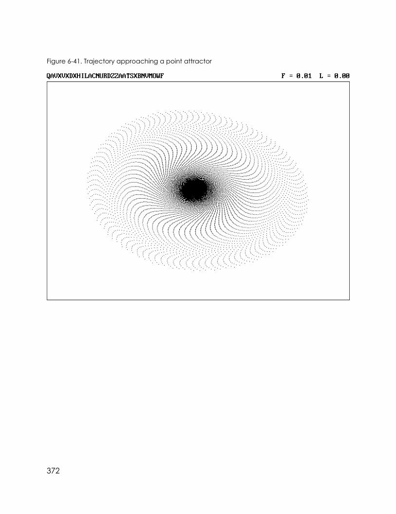
Figure 6-41. Trajectory approaching a point attractor
372

Figure 6-42. Trajectory approaching a point attractor
The point attractor is the simplest type of nonchaotic attractor. It has adimension of zero. An attractor can also have a dimension of one, which is a line.Such attractors are limit cycles. They correspond to systems that settle into aperiodic or cyclic behavior. Consequently, such attractors are also called cyclicattractors.
The simplest differential equations that produce a cyclic trajectory are theequations in Equation 6A. The resulting orbit is a circle in the XY plane. This case is notan attractor, however, because every initial condition produces a circular trajec-tory whose radius is the distance of the initial point from the origin. There is no uniquecircle to which nearby orbits are attracted, and there is no basin of attraction.Furthermore, if you attempt to display the trajectory using a code such asQM5NM5LM18, you will find that the orbit is unbounded and spirals outward as ifthere were a point repellor at the origin. The reason is that our iteration scheme for
373

approximating the solution of the differential equations is not exact. The errorscompound and eventually cause the orbit to be lost.
The simple undamped (frictionless) oscillator is said to be structurally unstablebecause an arbitrarily small perturbation to the equation (such as using the Eulerfinite difference approximation of Equation 6F) changes the structure of the solutionfrom a closed loop to a never-ending spiral. Note the distinction between anunstable equation, in which a small modification of the equation causes a largechange in the solution, and an unstable solution, in which a small variation of theinitial condition away from the equilibrium value causes the solution to move everfarther from equilibrium.
To produce a true limit cycle that is structurally stable, we need a system ofequations whose solutions spiral outward from initial conditions in the interior andspiral inward from initial conditions on the exterior of the attractor. A suitable set ofsuch equations is the following:
X’ = Y + (1 - X2 - Y2)X
Y’ = -X + (1 - X2 - Y2)Y (Equation 6H)
The quantity (1 - X2 - Y2) plays the role of -b in Equation 6G. Whenever the trajectorylies inside the circle of radius one, it spirals outward, and whenever it lies outside thecircle of radius one, it spirals inward. Thus the limit cycle is defined by the circle X2+ Y2 = 1. There is a point repellor at the origin, and the basin of attraction is the entireXY plane. A code that produces such a stable limit cycle, except with a smallerradius is RMNMAM3AM3NM9LM2AM6NMAM26.
A limit cycle may be either stable or unstable, just like a fixed point. With anunstable limit cycle, nearby orbits move progressively farther from the limit cycle. Anunstable limit cycle can be identified in an invertable map or system of ordinarydifferential equations by running time backwards, in which case the limit cyclebecomes stable and attracts rather than repels nearby orbits.
A slightly simpler version of Equation 6H that produces a stable limit cycle,although not a symmetrical one, is the following:
X’ = Y
Y’ = -X + (1 - X2)Y (Equation 6I)
This system is called the Van der Pol equation, and it was first used to model vacuum-
374
tube oscillator circuits, but it has been used in other applications such as themodeling of pulsating stars called Cephids. A code for the Van der Pol equation isRM11OM9KM2KM6OM28.
Such limit cycles are characterized by a dimension of one and a Lyapunovexponent of zero. The dimension as approximated by the program will usually notbe exactly 1.0 for the reasons discussed in Section 3.4. The Lyapunov exponent is amuch better criterion for identifying limit cycles. In a two-dimensional embeddingspace, as in the previous examples, there are two Lyapunov exponents. The smaller(more negative) of them is the rate at which trajectories with different initialconditions approach the attractor. The larger exponent (the one calculated by theprogram) is the rate at which two nearby points on the limit cycle separate. For alimit cycle produced by ODEs, this exponent must be zero because points along thetrajectory are governed by the same rates of flow, except delayed in time.
In two dimensions, the limit cycles cannot cross, so the most complicatedshapes are simple distorted loops. In three or more dimensions, they can wraparound in a complicated tangle like a ball of string, but without ends. Figures 6-43through 6-50 show a collection of visually interesting limit cycles. They are plottedas stereo pairs so that you can see how the trajectories pass beneath one another.
375

Figure 6-43. Limit cycle from a three-dimensional quadratic map
376

Figure 6-44. Limit cycle from a three-dimensional quadratic ODE
377

Figure 6-45. Limit cycle from three-dimensional quadratic ODE
378

Figure 6-46. Limit cycle from a three-dimensional quadratic ODE
379

Figure 6-47. Limit cycle from a three-dimensional cubic ODE
380

Figure 6-48. Limit cycle from a three-dimensional quintic ODE
381

Figure 6-49. Limit cycle from a four-dimensional quadratic ODE
382

Figure 6-50. Limit cycle from a four-dimensional quartic ODE
As you examine the figures, note that some of the limit cycles, such as the onein Figure 6-43, form knots. You cannot straighten them out into circular loops. Bycontrast, Figure 6-47 is unknotted. This knottedness or helicity is an importanttopological property of an attractor. Some processes in nature tend to conservehelicity, just as mechanical energy is conserved in frictionless motion. Thus whensome parameter of the system is changed, the limit cycle may change its size andshape but in such a way that it always links itself in the same way. An example is amagnetic field line in a turbulent conducting fluid such as a plasma of electricallycharged particles.
For many of the limit cycles exhibited here, it is very hard to tell whether theyare knotted. Even when they appear to be knotted, it is hard to tell whether twocases are knotted in the same way. Such patterns might provide a useful psycho-logical test for one’s spatial acuity because they require both depth perception
383

and a mental dexterity to visualize their shape when untangled as much as possible.See which of the limit cycles in the figures you think are knotted.
6.6 Doughnuts and Coffee Cups
Non-chaotic attractors can be points or lines. They can also be surfaces.Surfaces are two-dimensional manifolds. Perhaps the simplest set of equationswhose solution is a trajectory that fills a surface is the following:
X’ = Y
Y’ = -X
Z’ = aW
W’ = -Z (Equation 6J)
You will recognize the first two equations as the same as Equation 6A that producesa circle in the XY plane. The second two equations produce an ellipse in the ZWplane. The two motions are uncoupled (X and Y don’t depend on Z or W; Z and Wdon’t depend on X or Y). The parameter a is the square of the angular frequencyof the second motion. If the square root of a is a rational number (a ratio of twointegers) the trajectory is a closed one-dimensional loop in the four-dimensionalembedding space.
If the square root of a is irrational, the trajectory fills a two-dimensional toroidalsurface (called a 2-torus). The trajectory winds endlessly around the surface of adougnut, never intersecting itself. In such a case we say the frequencies (thenumber of transits per second the long way around and the short way around) areincommensurate and that the trajectory is quasi-periodic. The sequence neverrepeats, but it is not chaotic. It is sometimes difficult to distinguish between quasi-periodic and chaotic behavior.
A useful tool for distinguishing between a quasi-periodic and a chaoticattractor is the power spectrum of the time series, which has sharp peaks at discretefrequencies for quasi-periodic trajectories but a broad (continuous) spectrum forchaotic trajectories. The power spectrum contains about half of the informationrequired to reconstruct the trajectory; the frequency information is present, but thephase information is lost. Nevertheless, the power spectrum serves as a kind offingerprint that is very useful in categorizing attractors.
384
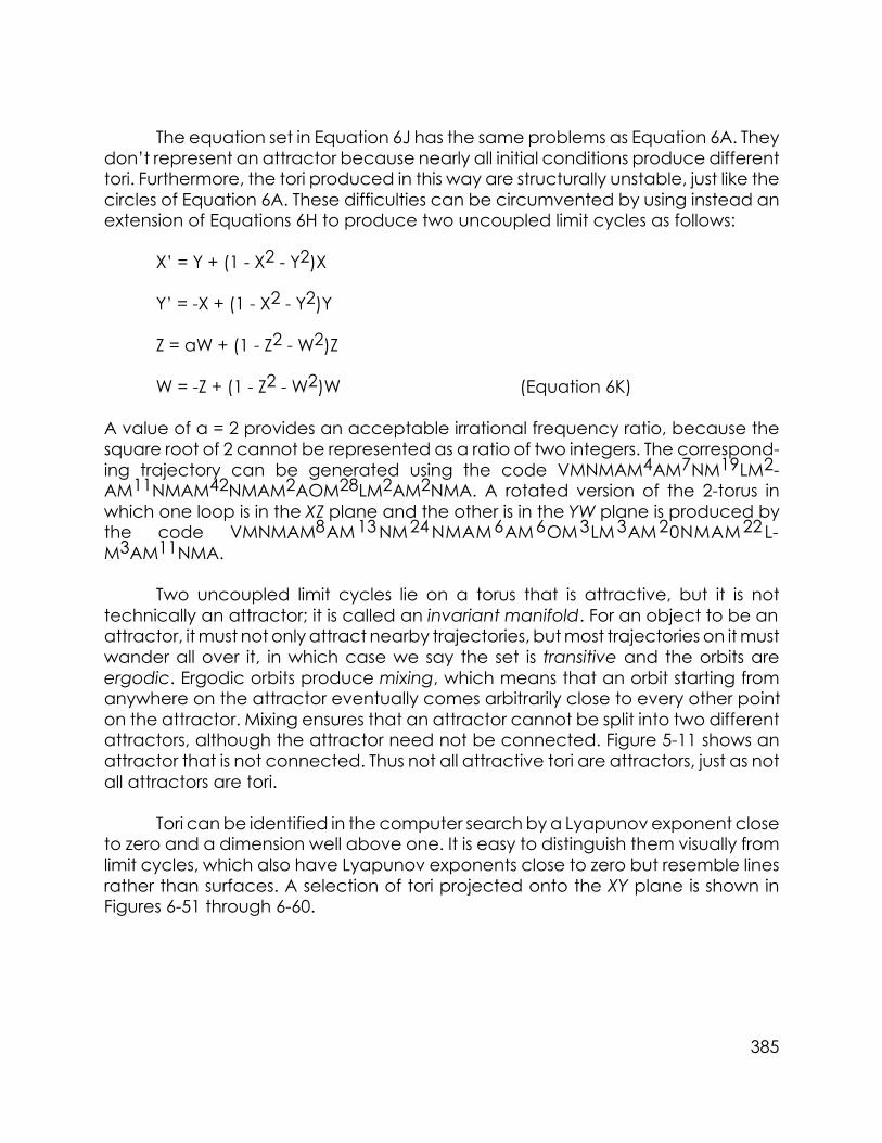
The equation set in Equation 6J has the same problems as Equation 6A. Theydon’t represent an attractor because nearly all initial conditions produce differenttori. Furthermore, the tori produced in this way are structurally unstable, just like thecircles of Equation 6A. These difficulties can be circumvented by using instead anextension of Equations 6H to produce two uncoupled limit cycles as follows:
X’ = Y + (1 - X2 - Y2)X
Y’ = -X + (1 - X2 - Y2)Y
Z = aW + (1 - Z2 - W2)Z
W = -Z + (1 - Z2 - W2)W (Equation 6K)
A value of a = 2 provides an acceptable irrational frequency ratio, because thesquare root of 2 cannot be represented as a ratio of two integers. The correspond-ing trajectory can be generated using the code VMNMAM4AM7NM19LM2-AM11NMAM42NMAM2AOM28LM2AM2NMA. A rotated version of the 2-torus inwhich one loop is in the XZ plane and the other is in the YW plane is produced bythe code VMNMAM8AM13 NM24 NMAM6AM6OM3LM 3AM20NMAM22 L-M3AM11NMA.
Two uncoupled limit cycles lie on a torus that is attractive, but it is nottechnically an attractor; it is called an invariant manifold. For an object to be anattractor, it must not only attract nearby trajectories, but most trajectories on it mustwander all over it, in which case we say the set is transitive and the orbits areergodic. Ergodic orbits produce mixing, which means that an orbit starting fromanywhere on the attractor eventually comes arbitrarily close to every other pointon the attractor. Mixing ensures that an attractor cannot be split into two differentattractors, although the attractor need not be connected. Figure 5-11 shows anattractor that is not connected. Thus not all attractive tori are attractors, just as notall attractors are tori.
Tori can be identified in the computer search by a Lyapunov exponent closeto zero and a dimension well above one. It is easy to distinguish them visually fromlimit cycles, which also have Lyapunov exponents close to zero but resemble linesrather than surfaces. A selection of tori projected onto the XY plane is shown inFigures 6-51 through 6-60.
385

Figure 6-51. Torus from a three-dimensional cubic ODE
386

Figure 6-52. Torus from Three-Dimensional Cubic ODE
387

Figure 6-53. Torus from a four-dimensional quadratic ODE
388

Figure 6-54. Torus from a four-dimensional quadratic ODE
389
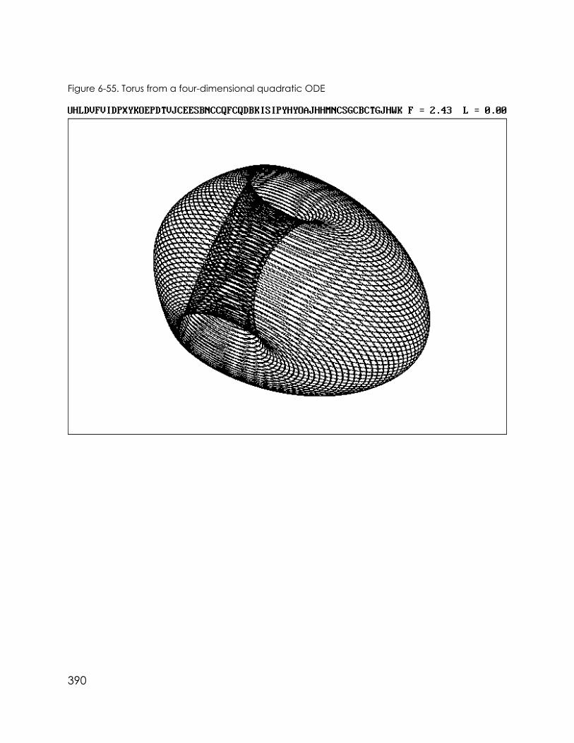
Figure 6-55. Torus from a four-dimensional quadratic ODE
390

Figure 6-56. Torus from a four-dimensional quadratic ODE
391

Figure 6-57. Torus from a four-dimensional quadratic ODE
392

Figure 6-58. Torus from a four-dimensional quadratic ODE
393
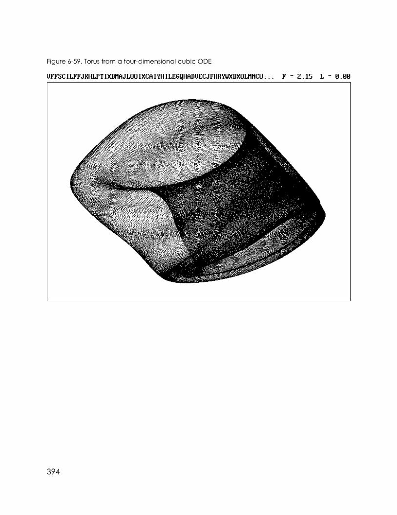
Figure 6-59. Torus from a four-dimensional cubic ODE
394

Figure 6-60. Torus from a four-dimensional quartic ODE
Most of the attractors shown in the figures look like tori in the sense that youcan see or imagine the hole in the doughnut. However, it is important to understandthat, just as not all limit cycles are circles, not all 2-tori look like doughnuts. They aretopologically equivalent in the sense that there is a "rubber-sheet" deformation(called a homeomorphism) that maps them into a doughnut. A coffee cup, forexample, is topologically equivalent to a doughnut as long as the handle isunbroken.
Those cases that are not obviously equivalent to a simple torus are distortedby the fact that they are viewed projected onto the XY plane or because they arerotated at an awkward angle. Also note that most of these tori are embedded ina four-dimensional space, so it is even more difficult to grasp their shape from a two-dimensional projection. You might want to display them using some of the ad-vanced visualization techniques provided by the program.
395
It is possible, though difficult, to produce a 3-torus in a four-dimensionalembedding space. A 3-torus is a generalization of a 2-torus. It is hard to visualize. Itinvolves three mutually incommensurate frequencies. It is characterized by adimension of three and a largest Lyapunov exponent of zero. Some of the attractorsin the figures seem to be 3-tori according to their calculated dimension. However,the calculation is not sufficiently precise to distinguish unambiguously between a 2-torus and a 3-torus. It is necessary to search embedding dimensions greater thanfour to have a good chance of finding 3-tori.
Dynamical systems whose trajectories lie on a 3-torus or other hypertori ofeven higher dimensions are difficult to observe in nature. The reason is that suchattractors can be perturbed by an arbitrarily small change to the system thatcauses them to become strange attractors. According to Peixoto’s theorem (whichstrictly applies only to compact, orientable manifolds), 2-tori tend to be structurallystable, while 3-tori and higher are structurally unstable. Thus it appears thatcomplicated deterministic systems that exhibit nontrivial behavior are well repre-sented by the strange attractors that constitute the subject of this book.
396

Chapter 7Further Fascinating Functions
For a system of equations to exhibit chaos, the equations must contain atleast one nonlinear term, that is, a term that is not simply proportional to one of thevariables. In all the preceding examples, the nonlinearity involved simple polynomi-als. Such polynomials are capable of modeling an enormous variety of physicalphenomena. Virtually all nonlinear functions can be approximated by polynomialswith sufficiently many terms. However, by limiting the polynomials to fifth order, wehave missed many interesting possibilities. In this chapter we examine a few of thesepossibilities and suggest others that you might want to explore on your own.
7.1 Steps and Tents
Perhaps the simplest nonlinear function is the absolute value, which isdenoted by |X| and programmed in BASIC with the command ABS(X). Theabsolute value of X is the magnitude of X without regard to its sign. For example, ifX is -6 then |X| is 6. It is a nonlinear function because a graph of |X| versus X is aV-shaped curve with its notch at the origin rather than a straight line as would resultif |X| were proportional to X. By adding linear terms, the V can be rotated toresemble an L or a staircase step. Computers can evaluate ABS(X) very quickly,since they only need to discard the sign.
An example of a one-dimensional chaotic map that involves |X| is the tentmap, so called because its graph is an inverted V. A tent map that maps the interval-1 to 1 back onto itself is
Xn+1 = 1 - 2|Xn| (Equation 7A)
The behavior of Equation 7A is very similar to the behavior of the logistic equation(Equation 1C) with R = 4, which maps the interval 0 to 1 back onto itself. A mappingthat returns a set onto itself is called an endomorphism.
Since one-dimensional maps tend not to be very interesting visually, we cangeneralize Equation 7A to two dimensions as follows:
Xn+1 = a1 + a2Xn + a3Yn + a4|Xn| + a5|Yn|
397

Yn+1 = a6 + a7Xn + a8Yn + a9|Xn| + a10|Yn| (Equation 7B)
This form is analogous to the general two-dimensional quadratic map in Equation3B.
To make things a little more interesting, we can add two more dimensions (Zand W) to take advantage of the visualization techniques that we have previouslydeveloped. However, to keep things simple, we will demand that X and Y notdepend on Z or W. They are just along for the ride, so to speak. The dynamicalbehavior is determined only by X and Y. We can choose any convenient equationfor Z and for W. One possibility is to evaluate Z from X and Y according to
Zn+1 = Xn2 + Yn
2 (Equation 7C)
Thus Z is the square of the distance of the previous iterate from the origin. You mightwant to experiment with other forms.
For the fourth dimension (W), we will do something completely different. Wewill arrange for W to increase linearly with the iteration number. Thus W becomes thetime coordinate in four-dimensional space-time.
The program modifications required to extend the computer search to suchcases are shown in PROG22. Codes for this case begin with the letter Y.
PROG22. Changes required in PROG21 to search for special functions of the Y type
1000 REM SPECIAL FUNCTION SEARCH (Steps and Tents)
1090 ODE% = 2 'System is special function Y
1710 IF ODE% > 1 THEN GOSUB 6200: GOTO 2020 'Special function
2670 IF ODE% > 1 THEN CODE$ = CHR$(87 + ODE%)
3650 IF ODE% > 1 THEN D% = ODE% + 5
398

3680 IF Q$ = "D" THEN D% = 1 + (D% MOD 7): T% = 1
3690 IF D% > 6 THEN ODE% = D% - 5: D% = 4: GOTO 3710
4290 IF ODE% > 1 THEN PRINT TAB(27); "D: System is 4-D special map "; CHR$(87+ ODE%); " ": GOTO 4320
4720 IF D% > 6 THEN ODE% = ASC(LEFT$(CODE$, 1)) - 87: D% = 4: GOSUB 6200: GOTO4770
6200 REM Special function definitions
6210 ZNEW = X * X + Y * Y 'Default 3rd and 4th dimension
6220 WNEW = (N - 100) / 900: IF N > 1000 THEN WNEW = (N - 1000) / (NMAX - 1000)
6230 IF ODE% <> 2 THEN GOTO 6270
6240 M% = 10
6250 XNEW = A(1) + A(2) * X + A(3) * Y + A(4) * ABS(X) + A(5) * ABS(Y)
6260 YNEW = A(6) + A(7) * X + A(8) * Y + A(9) * ABS(X) + A(10) * ABS(Y)
6270 RETURN
Examples of attractors produced by PROG22 are shown in Figures 7-1 through7-8. They are displayed as projections onto the XY plane to let you observe thehigher dimensional representations for the first time on your computer screen. Notethat these attractors differ from the cases produced by polynomials in that theytend to have sharp angular corners. The one in Figure 7-3 is not an attractor but isan example of an area-preserving system sometimes called the gingerbread manbecause of its shape.
399
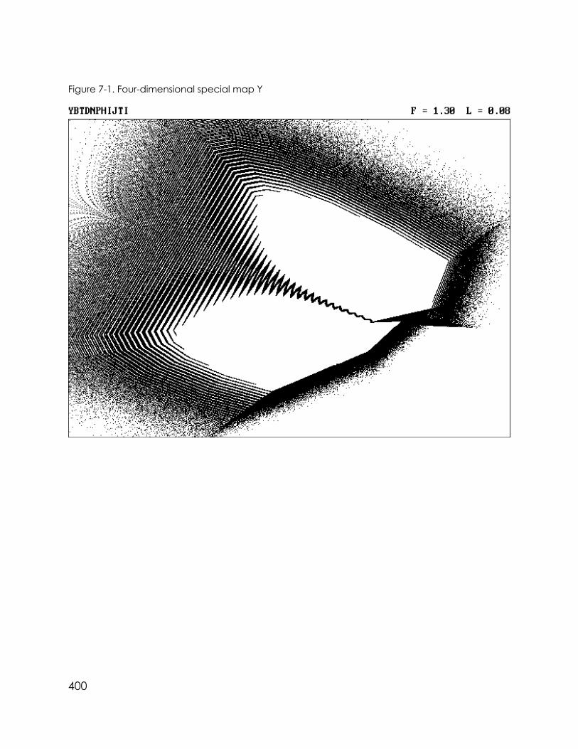
Figure 7-1. Four-dimensional special map Y
400

Figure 7-2. Four-dimensional special map Y
401

Figure 7-3. Four-dimensional special map Y (gingerbread man)
402

Figure 7-4. Four-dimensional special map Y
403
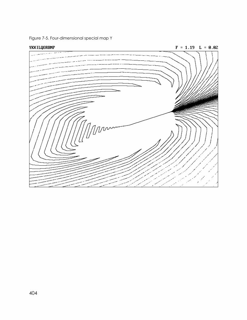
Figure 7-5. Four-dimensional special map Y
404

Figure 7-6. Four-dimensional special map Y
405

Figure 7-7. Four-dimensional special map Y
406

Figure 7-8. Four-dimensional special map Y
407

7.2 ANDs and ORs
A very different type of nonlinear map can be produced using logical(Boolean) operations to manipulate the individual bits of the binary numbers thatrepresent the variables. This is best done after rounding the variables to the nearestinteger using the BASIC CINT function. As a variation, you could use the FIX or INTfunction, both of which truncate rather than round. Most versions of BASIC auto-matically apply the CINT function before performing logical operations on numbersthat are not integers. The conversion of a noninteger to an integer is itself a nonlinearoperation, because the graph of CINT(X) versus X resembles a staircase.
The basic logical operators are AND and OR. If you are not sure what theseoperations mean, your BASIC manual is a good reference. The operation X AND Yproduces a new number whose bits are 1 if the corresponding bits of X and Y areboth 1, and 0 otherwise. The operation X OR Y produces a new number whose bitsare 1 if either (or both) of the corresponding bits of X or Y are 1, and 0 otherwise. Thisis also called the inclusive OR to distinguish it from the exclusive OR (XOR), whichproduces a number whose bits are 1 if either (but not both) of the correspondingbits of X or Y are 1, and 0 otherwise.
The following is a general two-dimensional system of equations that includesthe AND and OR operators:
Xn+1 = a1 + a2Xn + a3Yn + a4Xn AND a5Yn + a6Xn OR a7Yn
Yn+1 = a8 + a9Xn + a10Yn + a11Xn AND a12Yn + a13Xn OR a14 Yn
(Equation 7D)
The third and fourth dimensions are determined in the same way as in the previoussection.
The program modifications required to extend the computer search to suchcases are shown in PROG23. Codes for this case begin with the letter Z.
PROG23. Changes required in PROG22 to search for special functions of the Z type
1000 REM SPECIAL FUNCTION SEARCH (ANDs and ORs)
1090 ODE% = 3 'System is special function Z
408

3680 IF Q$ = "D" THEN D% = 1 + (D% MOD 8): T% = 1
6270 IF ODE% <> 3 THEN GOTO 6310
6280 M% = 14
6290 XNEW = A(1) + A(2) * X + A(3) * Y + (CINT(A(4) * X) AND CINT(A(5) * Y))+ (CINT(A(6) * X) OR CINT(A(7) * Y))
6300 YNEW = A(8) + A(9) * X + A(10) * Y + (CINT(A(11) * X) AND CINT(A(12) *Y)) + (CINT(A(13) * X) OR CINT(A(14) * Y))
6310 RETURN
Examples of attractors produced by PROG23 are shown in Figures 7-9 through7-16. Most of the attractors produced in this way have a streaked or checkeredappearance, arising presumably from rounding the variables to integers beforeperforming the logical operations. The ones shown in the figures tend to be theexceptions.
409

Figure 7-9. Four-dimensional special map Z
410

Figure 7-10. Four-dimensional special map Z
411

Figure 7-11. Four-dimensional special map Z
412

Figure 7-12. Four-dimensional special map Z
413

Figure 7-13. Four-dimensional special map Z
414

Figure 7-14. Four-dimensional special map Z
415

Figure 7-15. Four-dimensional special map Z
416

Figure 7-16. Four-dimensional special map Z
417

7.3 Roots and Powers
Polynomial maps involve powers of the variables that are small positiveintegers, such as the square (2) and the cube (3). Polynomials exclude suchnonlinearities as the square root or the reciprocal of the variables. Roots and powersare mathematically equivalent except for the value of the exponent. The squareroot of X can be written as X0.5, and the reciprocal of X can be written as 1/X or asX-1. It is interesting to examine strange attractors that involve fractional andnegative powers.
The following is a general two-dimensional system of equations that involvesarbitrary powers:
Xn+1 = a1 + a2Xn + a3Yn + a4|Xn|a5 + a6|Yn|a7
Yn+1 = a8 + a9Xn + a10Yn + a11|Xn|a12 + a13|Yn|a14
(Equation 7E)
The absolute values are needed because BASIC cannot take a root of a negativenumber. The result would have an imaginary component. Note that if all theexponents happen to be +1, Equation 7E is equivalent to Equation 7B. The third andfourth dimensions are determined in the same way as in Section 7.1.
The program modifications required to extend the computer search to suchcases are shown in PROG24. Since we have exhausted the capital letter codes, wemust invent some new ones. We will continue using the standard ASCII charactersbeyond Z, as shown in Table 2-1. Thus the codes for this case begin with the leftbracket ([), which is ASCII 91.
PROG24. Changes required in PROG23 to search for special functions of the [ type
1000 REM SPECIAL FUNCTION SEARCH (Roots and Powers)
1090 ODE% = 4 'System is special function [
3680 IF Q$ = "D" THEN D% = 1 + (D% MOD 9): T% = 1
6310 IF ODE% <> 4 THEN GOTO 6350
418
6320 M% = 14
6330 XNEW = A(1) + A(2) * X + A(3) * Y + A(4) * ABS(X) ^ A(5) + A(6) * ABS(Y)^ A(7)
6340 YNEW = A(8) + A(9) * X + A(10) * Y + A(11) * ABS(X) ̂ A(12) + A(13) * ABS(Y)^ A(14)
6350 RETURN
Examples of attractors produced by PROG24 are shown in Figures 7-17through 7-24. These attractors are localized mostly to a small region of the XY planewith tentacles that stretch out to large distances. If any of the exponents arenegative and the attractor intersects the line along which the respective variableis zero, a point on the line maps to infinity. However, large values are visitedinfrequently by the orbit, so many iterations are required to determine that the orbitis unbounded. For this reason most of the attractors in the figures have holes in theirinteriors where their orbits are precluded from coming too close to their origins (X =Y = 0).
419

Figure 7-17. Four-dimensional special map [
420

Figure 7-18. Four-dimensional special map [
421

Figure 7-19. Four-dimensional special map [
422

Figure 7-20. Four-dimensional special map [
423

Figure 7-21. Four-dimensional special map [
424
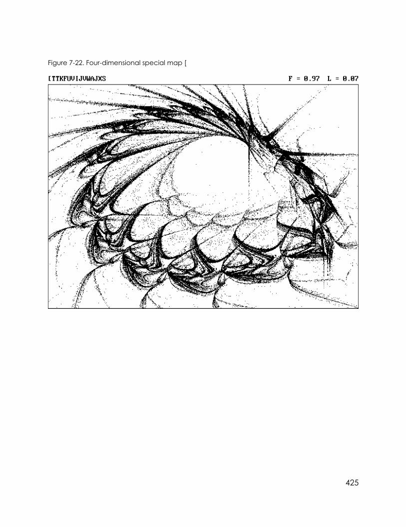
Figure 7-22. Four-dimensional special map [
425
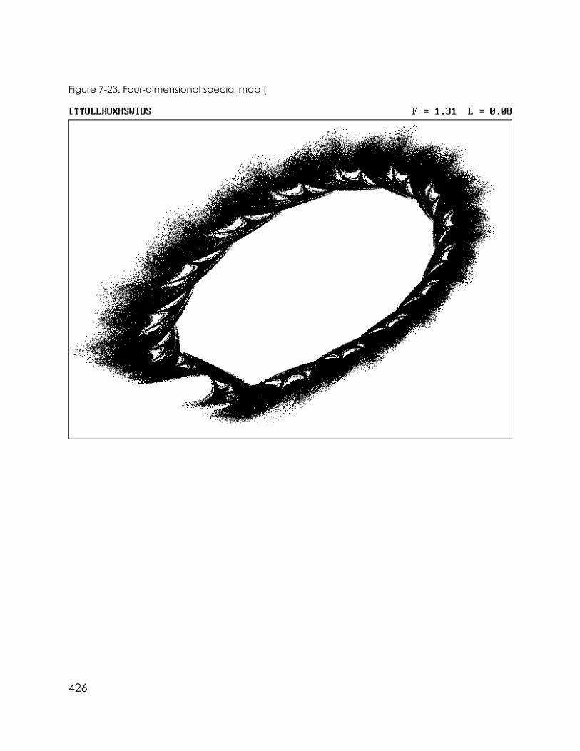
Figure 7-23. Four-dimensional special map [
426

Figure 7-24. Four-dimensional special map [
You may become frustrated seeing a beautiful attractor develop for thou-sands of iterations and then having the orbit escape. Such behavior is called a crisisor transient chaos, not to be confused with a catastrophe. For example, the logisticequation with R slightly greater than 4.0 is chaotic for many iterations until an iteratehappens to exceed 1.0, whereupon the orbit abruptly moves off toward infinity. Bycontrast, a catastrophe occurs when the solution undergoes a qualitative changeat some critical value of a control parameter.
Related to a crisis is another phenomenon called intermittency. At certainvalues of the control parameters, a system exhibits periodic behavior for manycycles and then suddenly becomes chaotic for a while before settling back intoperiodic behavior. Classic examples of intermittency occur in the logistic equationat about R = 3.82812 and in the Lorenz equations at about r = 166.2. Intermittencyhas been observed in many natural systems, and it is a bane to those who try to
427

make predictions. It is possible that the solar system is intermittently chaotic or eventhat a crisis can occur leading to a complete loss of its stability, perhaps precipi-tated by a rare conjunction of a planet with a large asteroid or comet.
Those solutions of Equation 7E that remain bounded tend to have a wispyappearance and to go beyond the frame of the figure because of the occasionallarge excursions. Artistically, this feature gives the attractors a sense of beingconnected to the surrounding world rather than being isolated objects suspendedin a void. If you frame these cases, a surrounding mat is desirable to provide theillusion that they are being viewed through a window.
7.4 Sines and Cosines
Two of the most common nonlinear functions are the sine and its comple-ment, the cosine. The sine and cosine can be approximated by polynomials asfollows:
sin X = X - X3/6 + X5 /120 - X7/5040 + ...
cos X = 1 - X2/2 + X4/24 - X6/720 + ... (Equation 7F)
When the argument X is small, the approximations are very accurate using only afew terms in the expansion. The denominator of each term is the factorial of theexponent of that term. For example, the factorial of five (written 5!) is equal to 5 x4 x 3 x 2 x 1 = 120. When X is large, many terms are required. In such a case, we wouldexpect to observe dynamics different from those produced by the fifth-orderpolynomials previously examined.
A general two-dimensional system of equations whose nonlinearity is re-stricted to the sine function is the following:
Xn+1 = a1 + a2Xn + a3Yn + a4sin(a5Xn + a6) + a7sin(a8Yn + a9)
Yn+1 = a10 + a11Xn + a12Yn + a13sin(a14Xn + a15) + a16sin(a17Yn + a18)
(Equation 7G)
It is not necessary to consider the cosine separately; the phase terms (a6, a9, a15,and a18) have the same effect because cos X is equal to sin(X + π/2). The third and
428

fourth dimensions are determined in the same way as in Section 7.1.
The program modifications required to extend the computer search to suchcases are shown in PROG25. These cases are coded with the backslash (\), whichis ASCII 92.
PROG25 Changes Required in PROG24 to Search for Special Functions of the \ Type
1000 REM SPECIAL FUNCTION SEARCH (Sines and Cosines)
1090 ODE% = 5 'System is special function \
3680 IF Q$ = "D" THEN D% = 1 + (D% MOD 10): T% = 1
6350 IF ODE% <> 5 THEN GOTO 6390
6360 M% = 18
6370 XNEW = A(1) + A(2) * X + A(3) * Y + A(4) * SIN(A(5) * X + A(6)) + A(7)* SIN(A(8) * Y + A(9))
6380 YNEW = A(10) + A(11) * X + A(12) * Y + A(13) * SIN(A(14) * X + A(15)) +A(16) * SIN(A(17) * Y + A(18))
6390 RETURN
Examples of attractors produced by PROG25 are shown in Figures 7-25through 7-32.
429

Figure 7-25. Four-dimensional special map \
430

Figure 7-26. Four-dimensional special map \
431

Figure 7-27. Four-dimensional special map \
432

Figure 7-28. Four-dimensional special map \
433
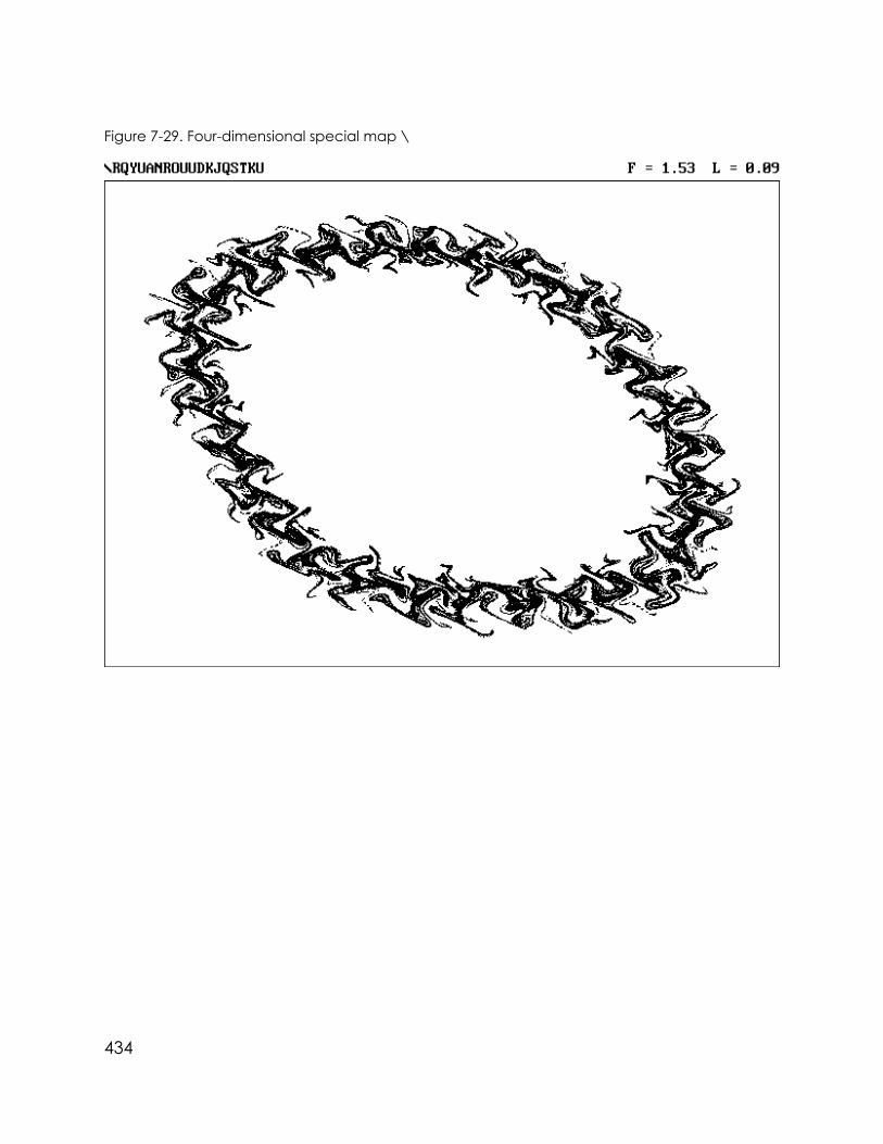
Figure 7-29. Four-dimensional special map \
434

Figure 7-30. Four-dimensional special map \
435
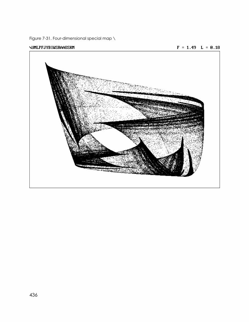
Figure 7-31. Four-dimensional special map \
436

Figure 7-32. Four-dimensional special map \
437

7.5 Webs and Wreaths
In this section, we consider a special type of map that involves sines andcosines. The solutions are chaotic, but they are not attractors. The systems theydescribe are Hamiltonian. Such Hamiltonian systems obey the Liouville theorem,which states that the phase-space volume occupied by a set of points is conservedas the system evolves in time. Thus the orbit eventually returns arbitrarily close to anyinitial condition. Contrast this to dissipative systems in which the phase-spacevolume decreases in time, eventually collapsing all initial conditions within the basinof attraction onto the attractor. In dissipative systems, the basin of attraction isusually much larger than the attractor. The equations are as follows:
Xn+1 = 10a1 + [Xn + a2sin(a3Yn + a4)]cos _ + Yn sin _
Yn+1 = 10a5 - [Xn + a2sin(a3Yn + a4)]sin _ + Yn cos _ (Equation 7H)
where α = 2π / (13 + 10a6). The third and fourth dimensions are determined in thesame way as in Section 7.1.
The special form of Equation 7H guarantees that the solution is not only area-preserving but also has circular symmetry. Furthermore, an inherent periodicityarises from the fact that α is 2π divided by an integer that ranges from 1 to 25. Theperiodicity is indicated by the last letter of the code (a6): A for period-1, B for period-2, and so forth. Because of the circular symmetry and infinite extent, it is interestingto project these cases onto a sphere using the P command.
The program modifications required to extend the computer search to suchcases are shown in PROG26. These cases are coded with the right bracket (]), whichis ASCII 93.
PROG26. Changes required in PROG25 to search for special functions of the ] type
1000 REM SPECIAL FUNCTION SEARCH (Webs and Wreaths)
1090 ODE% = 6 'System is special function ]
1150 TWOPI = 6.28318530717959# 'A useful constant (2 pi)
3680 IF Q$ = "D" THEN D% = 1 + (D% MOD 11): T% = 1
438

6390 IF ODE% <> 6 THEN GOTO 6450
6400 M% = 6
6410 IF N < 2 THEN AL = TWOPI / (13 + 10 * A(6)): SINAL = SIN(AL): COSAL = COS(AL)
6420 DUM = X + A(2) * SIN(A(3) * Y + A(4))
6430 XNEW = 10 * A(1) + DUM * COSAL + Y * SINAL
6440 YNEW = 10 * A(5) - DUM * SINAL + Y * COSAL
6450 RETURN
As you watch the patterns develop, you can see the orbit wander throughoutthe XY plane along a network of channels. The network is infinite in extent and iscalled a stochastic web. The global wandering is evidence of minimal chaos, andit causes the orbit eventually to leave the boundary of the computer screen. If youinterrupt the calculation at some point, the resulting structure resembles a wreathor a snowflake. The infinite structure is a tiling, but its symmetry is slightly spoiled bythe finite thickness of the web. This breaking of the symmetry eliminates themonotony and contributes to the aesthetic appeal of the patterns.
The slow wandering of the orbit throughout the web is an example of Arnol’ddiffusion, which is named after the Russian mathematician Vladimir Arnol’d. Nor-mally we associate diffusion with a random process in which, for example, themolecules of a gas move slowly from one region to another by countless collisionswith other molecules. The presence of diffusion in such simple deterministic systemshas many practical consequences such as providing a means for heating a gas ofelectrically charged particles (a plasma) in a magnetic field using electromagneticwaves.
These stochastic webs contain circular chains of islands, or beads on anecklace, if you prefer a different analogy, whose interiors contain periodic orbits.Surrounding the islands is a stochastic sea in which the orbits are chaotic andconnected to all other points in the sea. You will also note that the Lyapunovexponents are small. Since the orbits diffuse slowly in the sea, nearby orbits remainclose together for many iterations. For a similar reason, the calculated fractaldimension is lower than it should be. Recall that the dimension calculation is based
439

on the previous 500 iterates, whose values tend to be nearly equal in this case.
Examples of stochastic webs produced by PROG26 are shown in Figures 7-33through 7-40. Because of the slow diffusion of the orbit, these cases provide a goodopportunity to exhibit the time variation with colors as shown in Plates 31 and 32. Youmay want to try different values of NMAX% in line 1050 to control the rate at whichthe colors change. Web maps provide a perfect illustration of how chaos anddeterminism coexist. The underlying symmetry of the equations is evident in thefigures, but the orbit exhibits apparently random motion within the chaotic region.
Figure 7-33. Four-dimensional web map (period-4)
440

Figure 7-34. Four-dimensional web map (period-13)
441

Figure 7-35. Four-dimensional web map (period-5)
442

Figure 7-36. Four-dimensional web map (period-12)
443
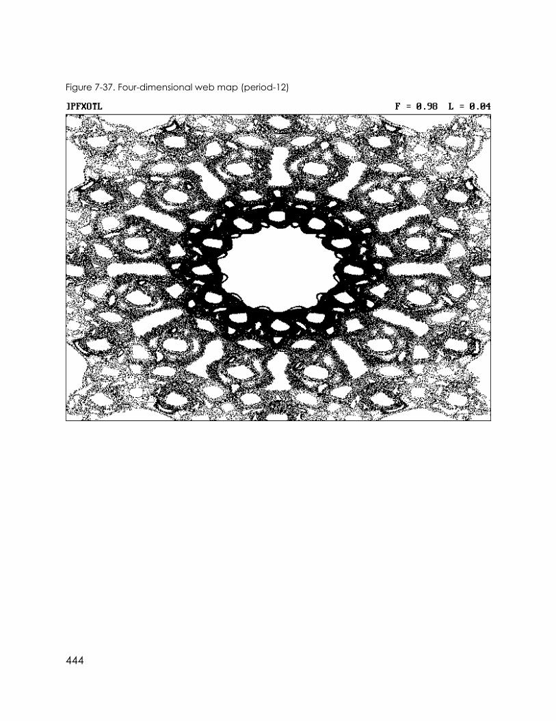
Figure 7-37. Four-dimensional web map (period-12)
444

Figure 7-38. Four-dimensional web map (period-7)
445

Figure 7-39. Four-dimensional web map (period-23)
446

Figure 7-40. Four-dimensional web map (period-9)
447

7.6 Swings and Springs
All the previous examples of maps and differential equations in this bookshare the property that the right-hand sides of the equations are independent ofthe iteration number (N) or time (t). Such equations are called autonomous. For agiven set of initial conditions, they produce the same solution for whatever time oriteration number they are started.
Some important physical processes are most conveniently expressed bynonautonomous equations. An example is a driven (forced), damped, linear,harmonic oscillator, which is described by the following equations:
X’ = Y
Y’ = -X - bY + A sin _t (Equation 7I)
In Equation 7I, b is the damping constant (friction), A is the amplitude of the drive(forcing) function, and ω is the angular frequency (radians per second) of the drive.The friction force is assumed to be proportional and opposite to the velocity (-Y),although other forms give qualitatively similar results. This type of friction is calledlinear damping.
The usual trick for dealing with nonautonomous equations is to introduce anadditional variable (say Z) and rewrite Equation 7I, for example, as
X’ = Y
Y’ = -X - bY + A sin Z
Z’ = _ (Equation 7J)
Equation 7J contains a nonlinearity (sin Z), but it does not have chaotic solutions. Thesolution (for positive b) is a limit cycle with frequency ω. The limit cycle is largest whenthe damping is small (b positive but much less than 1) and ω is 1, corresponding toresonance.
To obtain interesting chaotic solutions, we need additional nonlinear terms.We will restrict these nonlinearities to odd polynomials (X, X3, X2Y, and so forth) in theY’ equation to preserve the symmetry of the oscillation. A general form with oddpolynomials up to third order is as follows:
448

X’ = a1Y
Y’ = a2X + a3X3 + a4X2Y + a5XY2 + a6Y + a7Y3 + a8sin Z
Z’ = a9 + 1.3 (Equation 7K)
If the product a1a2 is negative, these equations represent the motion of a massoscillating on a nonlinear spring or a pendulum swinging through a large angle (butnot going over the top). If a3/a2 is positive, the spring gets stiffer when stretched orcompressed (hard spring). If a3/a2 is negative, the spring gets weaker whenstretched or compressed (soft spring). If a3/a2 is -1/6, the solution approximates avigorously swinging pendulum. If the product a1a2 is positive and a3/a2 is negative,the system models a buckled beam and is called the Duffing two-well oscillator. Thefinal combination (a1a2 and a3/a2 both positive) is unstable and has an un-bounded solution.
In Equation 7K, we can exploit the fact that Z enters only through the term sinZ; thus it is periodic with period 2π. Whenever Z exceeds 2π, we can subtract 2π fromit without changing the result. This trick keeps Z bounded in the range 0 to 2π ratherthan letting it march off to infinity as it would otherwise do. The Z-coordinate thenbecomes the phase angle of the drive function. Note that the MOD function in mostversions of BASIC works correctly only on integer variables, so it should not be usedfor the above purpose. The +1.3 term in the Z equation ensures that the phase anglealways increases in time for -1.2 ≤ a9 ≤ 1.2. The fourth variable (W) is proportional totime as in the previous examples.
The program modifications required to extend the computer search to suchcases are shown in PROG27. These cases are coded with the circumflex (^), whichis ASCII 94.
PROG27. Changes required in PROG26 to search for special functions of the ^ type
1000 REM SPECIAL FUNCTION SEARCH (Swings and Springs)
1090 ODE% = 7 'System is special function ^
3050 IF ODE% = 1 OR ODE% = 7 THEN L = L / EPS
449

3680 IF Q$ = "D" THEN D% = 1 + (D% MOD 12): T% = 1
6450 IF ODE% <> 7 THEN GOTO 6500
6460 M% = 9
6470 XNEW = X + EPS * A(1) * Y
6480 YNEW = Y + EPS * (A(2) * X + A(3) * X * X * X + A(4) * X * X * Y + A(5)* X * Y * Y + A(6) * Y + A(7) * Y * Y * Y + A(8) * SIN(Z))
6490 ZNEW = Z + EPS * (A(9) + 1.3): IF ZNEW > TWOPI THEN ZNEW = ZNEW - TWOPI
6500 RETURN
Examples of attractors produced by PROG27 are shown in Figures 7-41through 7-48. These cases are displayed as slices that show the orbit at 16 differentdrive phases. As you scan across them left to right and top to bottom, you can seethe stretching and folding that are characteristics of strange attractors and thataccount for their fractal microstructure and for the sensitivity to initial conditions.
450

Figure 7-41. Slices of a four-dimensional special map ^
451

Figure 7-42. Slices of a four-dimensional special map ^
452

Figure 7-43. Slices of a four-dimensional special map ^
453

Figure 7-44. Slices of a four-dimensional special map ^
454

Figure 7-45. Slices of a four-dimensional special map ^
455

Figure 7-46. Slices of a four-dimensional special map ^
456

Figure 7-47. Slices of a four-dimensional special map ^
457

Figure 7-48. Slices of a four-dimensional special map ^
These cases provide an ideal opportunity to animate the third dimension(drive phase). If you have not fanned through the figures in the upper-right-handcorner of the odd pages of the book, do so now. Be sure to fan in the forwarddirection (low to high page numbers). These figures were produced using 64 phaseslices of the attractor ^VYGJBPIJN with 10 million iterations.
You can see several cycles of stretching and folding. Note that there arethree diagonal bands that run from the lower left to the upper right of the attractor.The three bands are stretched and compressed into a single band, while twoadditional bands enter first from the upper left and then from the lower right. Thusone of the three bands consists of three smaller bands, one of which consists of threeeven smaller bands, and so forth. Such an infinitely layered band is called a thickline or a Cantor one-manifold. Viewed in three dimensions, the thick line wouldappear as a thick surface or a Cantor two-manifold. There is perhaps no clearer
458

illustration anywhere in this book of the way strange attractors are formed andacquire their fractal microstructure.
7.7 Roll Your Own
Perhaps this is a good place to leave you with this brief taste of the immensevariety of nonlinear functions and equations, nearly all of which admit strangeattractors that can be identified and examined using the technique described inthis book. The possibilities are limited only by your imagination, and you can beassured that nearly every strange attractor that you discover has never been seenbefore. There surely exist classes of objects yet to be discovered that are ofmathematical and artistic interest.
If you decide to pursue such an exploration, you might start with some of theother nonlinear functions and operators that are built into the BASIC language.Table 7-1 lists a number of interesting possibilities. They are divided into mathemati-cal functions, which should be independent of the machine or programminglanguage; machine functions, which are dependent on the machine or language;nonlinear operators, which are supported by nearly all versions of BASIC; andadvanced functions, which are supported by VisualBASIC for MS-DOS. You may usethem in combinations to invent complicated forms that belong to you alone!
Table 7-1. Nonlinear functions and operators supported by most versions of BASIC
Mathematical Machine Nonlinear AdvancedFunctions Functions Operators Functions
ABS FRE ^ DAYATN INP * HOURCINT PEEK / MINUTECOS PLAY \ MONTHEXP POINT MOD NOWFIX RND NOT QBCOLORINT TIMER AND RGBLOG OR SECONDSGN XOR WEEKDAYSIN EQV YEARSQR IMPTAN
459

Chapter 8Epilogue
It would be an injustice to leave you with the impression that the main use ofthe ideas in this book is to make pretty pictures. This final chapter describes some ofthe scientific applications of the method used to generate this large collection ofstrange attractors. It also suggests some additional explorations you might want toundertake as an extension of both the scientific and artistic aspects of the workdescribed in this book.
8.1 How Common is Chaos?
For hundreds of years, scientists have used equations like those in the previouschapters to describe nature. It is remarkable that almost no one recognized thechaotic solutions to those equations until the last few decades of the 20th century.Now researchers in many disciplines are beginning to see chaos under every rock.It is reasonable to wonder whether chaos is the rule or the exception.
Suppose we had a system of equations of sufficient complexity and withsufficiently many coefficients that it could be used to model most natural processes.We could then attempt to quantify the occurrence of chaos in these equations anddraw an inference about the occurrence of chaos in nature. The equations in theprevious chapters, especially those involving polynomials of high dimension andhigh order, might approximate such a system.
As a simple but very unrealistic example, suppose that all of nature could bemodeled by the logistic equation (Equation 1C). This equation has a single param-eter R that controls the character of the solution. If R is greater than 4 or less than -2, the solutions are unbounded, which means that this equation cannot model aphysical process under those conditions. Essentially all physical processes arebounded, except perhaps the trajectory of a spacecraft launched with sufficientvelocity to escape the galaxy. In the physically realistic range of R, there is a bandof chaos between about 3.5 and 4, as shown in Figure 1-2 and another identicalband between about -1.5 and -2. Careful analysis shows that chaos occurs overabout 13% of the range of R from -2 to 4.
Since the logistic equation is too simple a model for almost everything, weshould examine more complicated models. The Hénon map (Equation 3A) is a two-
460

dimensional generalization of the logistic map. It has two control parameters, whichnormally are a = -1.4 and b = 0.3. With b = 0, the Hénon map reduces to the logisticmap.
As with the logistic map, the Hénon map has unbounded solutions, chaoticsolutions, and bounded nonchaotic solutions, depending on the values of a and b.The bounded nonchaotic solutions may be either fixed points or periodic limitcycles. Figure 8-1 shows a region of the ab plane with the four classes of solutionsindicated by different shades of gray. The bounded solutions constitute an islandin the ab plane. On the northwest shore of this island is a chaotic beach, whichoccupies about 6% of the area of the island. The chaotic beach has many smallembedded periodic ponds. The boundary between the chaotic and the periodicregions is itself a fractal.
Figure 8-1. Regions of solutions for the Hénon map in the ab plane
461

The logistic map is chaotic over 13% of its bounded range, and the Hénonmap is chaotic over 6% of its bounded range. This result is counterintuitive becauseit suggests that more complicated (two-dimensional) systems are in some sense lesschaotic than simpler (one-dimensional) systems. Is this a general result, or is itpeculiar to these two maps? One way to decide is to examine a wider selection ofequations, such as the ones used to produce the attractors exhibited throughoutthis book.
In collecting attractors, we have been discarding interesting information—the number of bounded nonchaotic solutions for each chaotic case that theprogram finds. Discarding data is offensive to scientists, since experiments are oftenperformed with great effort and at considerable expense. The annals of scienceare ripe with examples of important discoveries that could have been made sooneror by others if only the right data had been recorded and analyzed.
Table 8-1 shows the results from 30,000 chaotic cases (1000 for each of the 30types) as identified by the program. This table includes over 400 million cases, ofwhich about 1 million are bounded. Of all the bounded solutions, 2.8% were chaoticaccording to the criterion described in Section 2.4. The polynomial maps all exhibita similar occurrence of chaotic solutions. The same is true of ordinary differentialequations (ODEs), but the percentage is smaller. The reason for this behavior is notunderstood.
Table 8-1. Summary of data from 30,000 chaotic cases
Code D O Type Chaotic Average F Average L
A 1 2 Map 3.34% 0.81±0.15 0.53±0.42
B 1 3 Map 5.09% 0.80±0.14 0.50±0.40
C 1 4 Map 8.09% 0.82±0.12 0.52±0.20
D 1 5 Map 7.94% 0.80±0.14 0.51±0.21
E 2 2 Map 7.58% 1.20±0.32 0.27±0.16
F 2 3 Map 7.08% 1.19±0.33 0.27±0.15
G 2 4 Map 6.40% 1.16±0.32 0.27±0.15
H 2 5 Map 5.79% 1.19±0.30 0.28±0.16
I 3 2 Map 6.68% 1.50±0.40 0.16±0.10
J 3 3 Map 5.89% 1.45±0.39 0.15±0.09
K 3 4 Map 5.08% 1.45±0.41 0.15±0.09
462

Code D O Type Chaotic Average F Average L
L 3 5 Map 4.68% 1.43±0.39 0.14±0.09
M 4 2 Map 4.99% 1.64±0.47 0.10±0.06
N 4 3 Map 4.78% 1.59±0.46 0.09±0.06
O 4 4 Map 5.32% 1.61±0.45 0.09±0.06
P 4 5 Map 5.04% 1.62±0.47 0.10±0.06
Q 3 2 ODE 0.55% 1.28±0.41 0.21±0.33
R 3 3 ODE 1.33% 1.31±0.40 0.73±0.76
S 3 4 ODE 1.23% 1.35±0.40 1.05±0.98
T 3 5 ODE 1.63% 1.38±0.41 1.23±1.16
U 4 2 ODE 1.34% 1.43±0.43 0.16±0.23
V 4 3 ODE 1.84% 1.43±0.43 0.40±0.48
W 4 4 ODE 1.84% 1.46±0.45 0.54±0.62
X 4 5 ODE 1.96% 1.44±0.44 0.66±0.76
Y 4 Special 16.28% 1.37±0.56 0.26±0.26
Z 4 Special 23.19% 1.03±0.44 0.28±0.44
[ 4 Special 16.00% 0.63±0.65 0.42±0.23
\ 4 Special 1.61% 1.10±0.28 0.16±0.10
] 4 Special 19.80% 1.02±0.16 0.06±0.04
^ 4 Special 1.91% 1.80±0.49 0.39±1.03
These results should not be taken too literally because the coefficients havebeen limited to the range -1.2 to 1.2, the ODEs have not been solved veryaccurately, and many cases are ambiguous. Chaotic solutions tend to occur atlarge values of the coefficients where most of the solutions are unbounded. A morecareful evaluation, which corrects these difficulties and includes about 35,000strange attractors but limited to fewer types, shows that the probability that abounded solution is chaotic for an iterated polynomial map of dimension D andorder O is given approximately by
P = 0.349 D-1.69 O-0.28 (Equation 8A)
Similarly, the probability that a bounded solution is chaotic for a polynomial ODE of
463
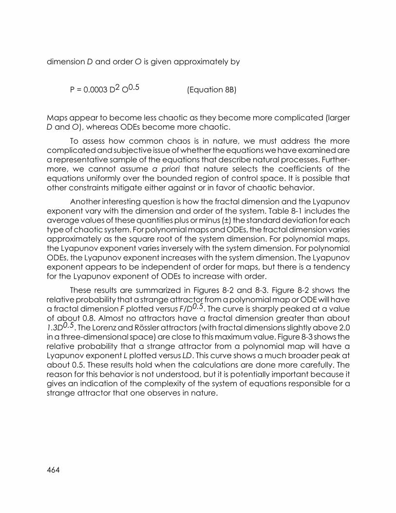
dimension D and order O is given approximately by
P = 0.0003 D2 O0.5 (Equation 8B)
Maps appear to become less chaotic as they become more complicated (largerD and O), whereas ODEs become more chaotic.
To assess how common chaos is in nature, we must address the morecomplicated and subjective issue of whether the equations we have examined area representative sample of the equations that describe natural processes. Further-more, we cannot assume a priori that nature selects the coefficients of theequations uniformly over the bounded region of control space. It is possible thatother constraints mitigate either against or in favor of chaotic behavior.
Another interesting question is how the fractal dimension and the Lyapunovexponent vary with the dimension and order of the system. Table 8-1 includes theaverage values of these quantities plus or minus (±) the standard deviation for eachtype of chaotic system. For polynomial maps and ODEs, the fractal dimension variesapproximately as the square root of the system dimension. For polynomial maps,the Lyapunov exponent varies inversely with the system dimension. For polynomialODEs, the Lyapunov exponent increases with the system dimension. The Lyapunovexponent appears to be independent of order for maps, but there is a tendencyfor the Lyapunov exponent of ODEs to increase with order.
These results are summarized in Figures 8-2 and 8-3. Figure 8-2 shows therelative probability that a strange attractor from a polynomial map or ODE will havea fractal dimension F plotted versus F/D0.5. The curve is sharply peaked at a valueof about 0.8. Almost no attractors have a fractal dimension greater than about1.3D0.5. The Lorenz and Rössler attractors (with fractal dimensions slightly above 2.0in a three-dimensional space) are close to this maximum value. Figure 8-3 shows therelative probability that a strange attractor from a polynomial map will have aLyapunov exponent L plotted versus LD. This curve shows a much broader peak atabout 0.5. These results hold when the calculations are done more carefully. Thereason for this behavior is not understood, but it is potentially important because itgives an indication of the complexity of the system of equations responsible for astrange attractor that one observes in nature.
464

Figure 8-2. Probability distribution of fractal dimension
465

Figure 8-3. Probability distribution of Lyapunov exponent
The similarity of the fractal dimension for attractors produced by polynomialsof the same dimensionality raises the concern that they might in some sense all bethe same attractor, viewed from different angles and distorted in various ways.There may be a simple mapping that converts one attractor into the others. In sucha case, a statistical analysis of the collection would be misleading and meaningless.However, since the Lyapunov exponents are spread over a broad range, it seemslikely that the attractors are distinct. In any case, they are visually very different, andthus the technique has artistic if not scientific value.
It is interesting to ask whether the above results are peculiar to polynomials.Table 8-1 includes data for the special functions that were described in Chapter 7.Some of these cases tend to be more chaotic than the polynomials, but thedifferences are not enormous. Thus is would appear, insofar as nature can berepresented by systems of equations of the type described in this book, that chaos
466

is not the most common behavior, but neither is it particularly rare.
8.2 But Is It Art?
A very different question is whether pictures generated by solving determin-istic equations with a computer can legitimately qualify as art. Some people wouldsay that if it was done by a computer without human intervention, it cannot be art.On the other hand, humans chose the equations, built and programmed thecomputer, decided how the solution would be displayed, and selected from thelarge number of cases that the computer generated. In this view, the computer isjust another tool in the hands of the artist.
At the core of the issue is what we mean by art. There are at least two, notnecessarily mutually incompatible, views. One is that art is the expression of ideasand emotions—a form of communication between the artist and the observer. Theother emphasizes formal design, in which the viewer admires the skill with which theartist manipulated the materials, without reading any particular meaning into it.
Strange attractors qualify by either definition. They are expressions of ideasembodied in the equations, whether it be the dynamics of population growth or aswinging pendulum. These ideas are often abstract and are most apparent to thetrained mathematician or scientist, but anyone can see in the patterns the surrealimages of plants, animals, clouds, and swirling fluids. The appearance of suchfamiliar images in the solutions of mathematical equations is probably more thancoincidental.
Strange attractors also necessarily embody concepts of design. The interplayof determinism and unpredictability ensures that they are neither formless norexcessively repetitious. Furthermore, the skills of an artisan (if not an artist) arerequired to translate the abstract equations into aesthetically desirable visual forms.These skills are different from (but not inferior to) those possessed by more conven-tional artists. Renaissance artists, such as Leonardo da Vinci, were often alsoscientists. We may now be entering a new Renaissance in which art and science areagain being drawn together through the visual images produced by computers.
Some artists view art as a creative process whose primary goal is to providethe artist with a sense of satisfaction. The resulting work is merely an inevitable by-product. This view seems especially appropriate for the production of strangeattractors, where the programmer’s satisfaction is derived from causing the com-puter to generate the patterns, even if they are never seen by anyone else. Indeed,the computer offers the ideal medium for such conceptual artists, since there needbe no material product whatsoever.
467

Note that visual art need not be beautiful to be good, just as a play need notbe humorous. It may be intellectually or emotionally satisfying, or even disturbing.It should capture and hold the interest of the viewer, however. The span of theviewer’s attention is one measure of its quality. Art may mix the familiar and theunfamiliar to produce both comfort and dissonance. Furthermore, beauty is at leastpartially in the eye of the beholder, although recent research indicates that thereare absolute universal measures of beauty that form very early in life and may evenbe genetic.
8.3 Can Computers Critique Art?
The idea that a computer can make aesthetic judgments seems absurd andeven offensive to many people. Yet the program developed in this book is alreadydoing this to some degree. For every object (strange attractor) that it identifies, ithas discarded many dozens as being uninteresting (nonchaotic). Perhaps thecomputer could be programmed to be even more discriminating and to selectthose strange attractors that are likely to appeal to humans. To the extent thataesthetic judgment involves objective as well as subjective criteria, such a propo-sition is not unreasonable.
A computer lacks emotion, but it can be taught in much the same way thatpeople can be taught. With the help of a human to point out which attractors arevisually interesting, the computer can correlate human opinion with various quan-titative measures of the attractor. It can then test each new case and assign aprobability that it would appeal to a human.
One of the reasons we have been calculating and saving the fractaldimension and Lyapunov exponent for each strange attractor is in anticipation ofdeveloping such criteria. You can think of the dimension as a measure of thestrangeness of an attractor and the Lyapunov exponent as a measure of itschaoticity. These are just two of infinitely many independent quantities we can useto describe each attractor. If we find encouragement from them, it suggests thatmore can be done.
The first step is to search for a relation between the aesthetic quality and thefractal dimension or Lyapunov exponent. For this purpose, 7500 strange attractorsfrom two-dimensional quadratic maps were evaluated by the author and sevenvolunteers, including two graduate art students, a former art history major, threephysics graduate students, and a former mathematics major. All evaluators wereborn and raised in the United States. The evaluations were done by choosingattractors randomly and displaying them sequentially on the computer screenwithout any indication of the quantities that characterize them. The volunteerswere asked to evaluate each case on a scale of one to five according to its
468

aesthetic appeal. It only took a few seconds for each evaluation.
Figure 8-4 displays a summary of all the evaluations as a function of fractaldimension (F) and Lyapunov exponent (L), using a gray scale in which the darkerregions are the most highly rated. The cases examined by particular individualsshow a similar trend. All evaluators tended to prefer attractors with dimensionsbetween about 1.1 and 1.5 and Lyapunov exponents between zero and about 0.3.Some of the most interesting cases have Lyapunov exponents below about 0.1. Yousaw many such examples earlier in this book.
Figure 8-4. Regions of highest aesthetic quality in the FL plane
469

The dimension preference is not surprising, since many natural objects havedimensions in this range. Nature is strange, but usually not totally bizarre. Some of theattractors that are most universally liked resemble well-known and easily recogniz-able objects. You can find many such examples in this book.
The Lyapunov exponent preference is harder to understand, but it suggeststhat strongly chaotic systems are too unpredictable to be appealing. For the 443cases that were rated 5 (best) by the evaluators, the average dimension was F =1.30 ± 0.20, and the average Lyapunov exponent was L = 0.21 ± 0.13 bits periterations, where the errors represent plus or minus one standard deviation. About28% of the cases evaluated fall within both error bars. Thus this simple criterion wouldallow the computer to discard nearly three-quarters of the cases that are least likelyto be visually appealing. This technique works in practice and was used in somecases to help select attractors to display in this book.
8.4 What’s Left to Do?
This book has described a new technique for generating strange attractorsin unlimited numbers. A large collection of such objects offers many interestingpossibilities to the artist and scientist alike. Some of these uses have already beenmentioned. Others may have occurred to you as you read this book. This sectionleaves you with a few additional suggestions of things you might want to explore onyour own.
If your main interest is art, you probably want to produce attractors withimproved spatial resolution and more colors. You can experiment with printing ondifferent types of paper or other media. The simple linear correspondence of X, Y,Z, and W to position or color is not essential. Other mappings between themathematical variables and the points displayed on the screen are possible. Youhave already seen how to project the attractors onto a sphere. You can projectthem onto other objects such as cylinders, tori, or even other strange attractors.
When you have generated an attractor that appeals to you, it is natural towant to make small changes to make it even better. The coefficients in theequations are controls that you can adjust. Like knobs on your television set, theyallow you to tune the attractor to get just what you want. You can change the colorswithout replotting the data using the PALETTE command in BASIC. You also canrotate the image to find the best angle from which to view it.
You can produce animated strange attractors with a video camera viewinga monitor connected to the camera, or even more simply, with a photodiodeconnected to an oscilloscope whose screen illuminates the photodiode. This video-
470

feedback technique has much in common with iterated maps. Each illuminateddot on the screen is mapped back to a different location after a delay determinedby the propagation of the electrical and optical signals. The main control param-eters are the distance, rotation, focusing, intensity, color, and hue. Some settingsproduce unbounded solutions—the screen goes solid black or solid white. Othersettings produce a fixed-point solution with a stationary pattern. Under otherconditions, periodic behavior occurs. The most interesting situation occurs whenthe pattern constantly changes but is not periodic, corresponding to a chaoticstrange attractor. Sometimes you can perturb the system with a flash of light or bymoving your hand across the field of view, causing the system to switch from oneattractor to another.
Some of the most interesting examples of computer fractals come fromplotting the basin boundaries of various attractors. The basin is the set of all initialconditions that are drawn to the attractor. Sometimes these boundaries aresmooth; other times they are fractals. By coloring the points just outside the basinaccording to the number of iterations required for them to leave some (usuallylarge) region surrounding the attractor, beautiful escape-time fractal patterns canbe produced.
All of our attractors have such basins, and it’s not hard to program thecomputer to display them, but the calculations are very slow. As an example, Figure8-5 shows in black the basin for the Hénon map. It is relatively smooth and notparticularly interesting. It resembles a thick version of the attractor, but rotated by90 degrees. Figure 8-6 shows the basin of another two-dimensional quadratic mapcalled the Tinkerbell map. Its boundary has obvious fractal structure. In each case,the basin boundary appears to touch the attractor, suggesting that this surprisingfeature may be common.
471

Figure 8-5. Basin of attraction for the Hénon map
472
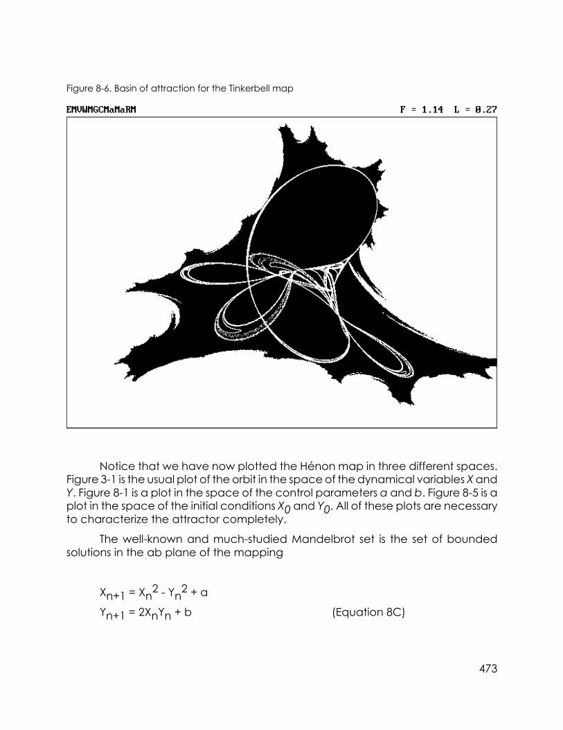
Figure 8-6. Basin of attraction for the Tinkerbell map
Notice that we have now plotted the Hénon map in three different spaces.Figure 3-1 is the usual plot of the orbit in the space of the dynamical variables X andY. Figure 8-1 is a plot in the space of the control parameters a and b. Figure 8-5 is aplot in the space of the initial conditions X0 and Y0. All of these plots are necessaryto characterize the attractor completely.
The well-known and much-studied Mandelbrot set is the set of boundedsolutions in the ab plane of the mapping
Xn+1 = Xn2 - Yn
2 + a
Yn+1 = 2XnYn + b (Equation 8C)
473

The variables X and Y usually are thought of as the real and imaginary parts of acomplex number Z. Each point in the ab plane has associated with it a Julia set,which is the set of all initial conditions X0 and Y0 whose solutions are bounded. TheMandelbrot set is the set of Julia sets every point of which is connected to everyother point. The Julia set is named after Gaston Julia, a French mathematician who,along with Pierre Fatou, studied iterated maps in the complex plane at about thetime of the first world war. Combinations of a and b at the boundary of theMandelbrot set produce chaotic solutions, but values inside the set lead to fixedpoints or limit cycles. For b = 0 and Y0 = 0 (the real axis), Equation 8C reduces to asimple one-dimensional quadratic map equivalent to the logistic map.
The Mandelbrot set has been described as the most complicated math-ematical object ever seen. It may also be the ultimate computer virus, in that it takesover not only the machine (because of the large computational requirements) butalso the mind of the programmer, who often becomes addicted to the beauty andvariety of the patterns that it produces.
Like the Mandelbrot set, most of the attractors produced by the programs inthis book have intricate structure near the basin boundaries. You can zoom in onthese regions to produce patterns that rival those produced by the Mandelbrot set.Calculation times increase markedly as you zoom in ever more closely, however.
Much more can be done to correlate the aesthetic appeal of the attractorswith the various numerical quantities that characterize them. Besides the fractaldimension and Lyapunov exponent, the system that produced them has dimensionand order. Other measures of an attractor’s dimension include the capacitydimension, the information dimension, and the Lyapunov dimension. Related to theLyapunov exponent is the entropy, which is a measure of the disorder of the system.As with the dimension, the entropy can be defined in many ways. These quantitiesand others are described in many of the books on fractals in the bibliography. Mapsand differential equations can also be compared.
You can test for differences between the aesthetic preferences of artists andscientists. Preliminary indications suggest that complexity might appeal more toartists than to scientists, who tend to see beauty in simplicity. There may also bediscernible cultural differences. You can see how the various display techniquesalter one’s preferences. For example, the use of color seems to increase thetolerance for attractors of high fractal dimension.
Many scientific studies can be performed on a sufficiently large collection ofstrange attractors. The results of Table 8-1, which are merely suggestive and limitedto particular types of equations, can be refined with more cases and moreexamples of each case. For low dimensions, maps are more chaotic than theequivalent ODEs. As the system dimension increases, however, maps become lesschaotic, while ODEs become more chaotic. Equation 8A and 8B suggest that for a
474
system dimension of about six, maps and ODEs will be equally chaotic. Will their rolesreverse at higher dimension, or will the chaotic fractions asymptotically approacha universal value of about 2%?
You can ask the same type of questions about bounded, nonchaoticsolutions (fixed points, limit cycles, and tori). It is especially interesting to see howcommon 3-tori are in light of Peixoto’s theorem (see Section 6.6), but their produc-tion probably requires system dimensions of about 10 according to Figure 8-2, whichmay or may not apply to tori. Almost nothing is known about such issues.
We have considered the fraction of the bounded, hyperdimensional controlspace over which chaos occurs. It is also interesting to examine the shape, location,and dimension of this chaotic region, as we did for the two-parameter Hénon mapin Figure 8-1. It is likely that this region is a fractal. How does its fractal dimensiondepend on the system dimension and other characteristics of the system ofequations? It appears that the dimension of the chaotic region is about half thedimension of the control space for the cases in this book.
The scaling of the average fractal dimension and the Lyapunov exponentwith the system dimension is intriguing and should be studied with more cases,better statistics, and more accurate calculations of the fractal dimension. You canexamine statistically how the various measures of dimension compare and howthese dimensions are related to the spectrum of Lyapunov exponents.
You can look for relations between the geometrical properties of attractorsand their respective power spectra. The technique can be used to explore and toquantify the various routes by which a stable solution becomes chaotic. Many suchroutes have been identified, such as the period-doubling exhibited by the logisticequation, but there are probably others yet to be discovered. Your role resemblesthat of a biologist confronted with a large variety of species, trying to classify,quantify, and study their similarities, differences, and patterns of behavior.
Another interesting study is to search for previously unknown simple examplesof chaos. Variations of the logistic equation are the simplest chaotic polynomialmaps. The Lorenz and Rössler attractors are often cited as the simplest examples ofchaotic polynomial ODEs. The Lorenz equations (Equation 6D) have seven termsand two quadratic nonlinearities, and the Rössler equations (Equation 6E) haveseven terms and one quadratic nonlinearity.
There are at least five different systems of chaotic, three-dimensional qua-dratic ODEs with five terms and two nonlinearities, and six systems with six terms andone nonlinearity. It will be left as a challenge for you to find them. There does notseem to be any chaotic system of quadratic ODEs with as few as four terms. To whetyour appetite, here’s a simple chaotic system resembling the Lorenz attractor thathas two fewer terms and all its coefficients equal to one:
475

X' = YZ
Y' = X -Y
Z' = 1 - XY (Equation 8D)
You can examine this case using the code QM7NM3NM3LM4NM2LM6.
Here’s another case with five terms and all unity coefficients that’s volume-preserving and thus does not have an attractor, but its solution is either a 2-torus orchaotic depending upon the initial conditions:
X' = Y
Y' = X + YZ
Z" = 1 - Y2 (Equation 8E)
It can be produced with the code QM5NM5LM5NM2NM5LM3.
8.5 What Good Is It?
It is rare that a mathematical concept captivates the interest not only ofscientists in diverse fields but of the general public. Chaos has done this, and it hasbeen heralded by some as the next great revolution in science. It has ushered in anew field of experimental mathematics, sometimes pejoratively called recre-ational mathematics by the more traditional and often cynical older breed ofmathematicians. The use of computers to produce exotic visual patterns has madedifficult mathematical ideas accessible to those without extensive formal training.
Yet it is fair to ask what it has done other than to make pretty pictures. Oneresponse is to claim that the same things were probably said about the discoveryof the atomic nucleus, or electricity, or fire. We must have faith that intellectualadvances will eventually yield useful applications.
At the deepest level, an understanding of chaos alters our view of the world.Having seen the complexity that can arise from simple equations, we have reasonto hope that simple equations may suffice to describe much of the complexity ofthe world. Difficult and long-standing problems such as fluid turbulence mayeventually be understood using the ideas of chaos. Turbulence is difficult becauseit involves both temporal and spatial chaos and because its dimension is high.
476

Chaos may also provide tools for making better predictions of complicated andapparently random systems, such as the weather, the stock market, earthquakes,epidemics, and population growth. It may also have applications in communica-tions and in cryptography for devising secure codes and breaking them.
Since chaotic systems exhibit extreme sensitivity to initial conditions, youmight conclude that prediction is hopeless, but this is not the case. Prediction ishopeless for a random system or for an extremely complicated deterministicsystem. As the physicist Neils Bohr remarked, "Prediction is difficult, especially of thefuture." However, if the system is simple and chaotic, then the determinism can beexploited to improve short-term predictions.
Furthermore, if the equations produce a strange attractor, as most chaoticsystems do, we know that the solution lies somewhere on the attractor. Rememberthat an attractor occupies a negligible volume of the space in which it is embed-ded. Although we can’t predict where on the attractor the system will be at anyparticular time in the distant future, we can exclude the vast number of possiblestates that lie off the attractor. In meteorological terms, this might lead to eliminat-ing the possibility of certain weather conditions with near absolute certainty.
When we see a system in nature that behaves erratically, we are now led towonder whether it is an example of chaos. Is simple determinism hidden inseemingly random data? This problem is opposite to the one addressed in this book.Here we have started with simple equations and produced complicated patterns.Nature presents us with complicated patterns that may or may not come fromsimple equations.
Often we are given only a single fluctuating quantity sampled at discretetimes—a so-called time series. The average daily temperature in New York and thedaily closing Dow Jones Industrial Average are two examples of a time series.Sometimes a complicated-looking time series is simply a sum of several sine wavesof different unrelated frequencies. In such a case, accurate predictions arepossible using linear methods. A good example is the tides, whose behavior is notsimply periodic but nevertheless can be predicted with considerable accuracybecause it is governed by periodic notions of the earth and moon. More often, thetime series has no such simple representation. In such a case, we would like todetermine whether the behavior is random or chaotic. Chaotic systems oftenproduce strange attractors.
We usually don’t have data for all the variables that describe the system, nordo we even know how many there are, so we don’t know the dimension of thespace in which an attractor might be embedded. Furthermore, the data record islikely to be corrupted by random noise and measurement errors. The number ofdata points may be small, and the system may not have reached a steady state.Finally, we usually don’t have control over the system, so we cannot directly test its
477

sensitivity to initial conditions.
Such a situation sounds hopeless, but progress has recently been made intesting for chaos in natural systems. For example, one can plot each data pointversus its predecessor, as we did with the one-dimensional maps in Chapter 2. Insome cases, this procedure is enough to reveal the determinism. More often, it isnecessary to plot each data point versus several of its predecessors in a high-dimensional space. If the system is described by a strange attractor, the result is aversion of the attractor called a diffeomorphism that is distorted but has the samefractal dimension. Similarly, the Lyapunov exponent can be estimated by selectingnearby points in this space and determining how rapidly they diverge from oneanother.
The fractal dimension is important because the number of variables andequations is at least as large as the next higher integer, since the attractor has to beembedded in a space with dimension higher than its fractal dimension. Theseequations are not unique, however. Extracting equations from the data is a difficultif not impossible task, but one whose rewards justify the effort. The equations provideinsight into the underlying dynamics and a means for making predictions.
Perhaps the ultimate test for chaos is the accuracy of short-term predictions.With truly random data, prediction is impossible. Conversely, with chaotic data,there is absolute determinism, and prediction is possible in principle, at least onshort-time scales dictated by the Lyapunov exponent and the precision of thedata. Predictability thus precludes complete randomness and signifies determin-ism, although randomness and determinism often coexist. For example, the busi-ness cycle is mostly random but includes deterministic seasonal changes. Thedeterministic part is not necessarily chaotic, however.
Dynamical systems are everywhere. Your body contains several. Your heartis a dynamical system whose solution normally approaches a limit cycle, but whichcan become chaotic when in fibrillation or a fixed point upon death. Recentresearch suggests that even a healthy heart beats chaotically, and a nearlyperiodic pattern sometimes precedes cardiac arrest.
Other oscillations occur in your lungs, brain, and muscles. Electrocardio-grams and electroencephalograms are time-series records used by doctors todeduce information about the dynamics of the corresponding organ. Some chaosin the brain may be necessary for creativity because it prevents us from repeatedlyapproaching the same problems in the same way. The fractal dimension ofelectroencephalograms has been observed to increase when a subject is en-gaged in mental activity. In psychology, manic depression resembles a limit cycle,and certain types of erratic behavior might be strange attractors.
Evidence for low-dimensional strange attractors has been found in systems
478

as diverse as the weather and climate, the business cycle, childhood epidemics,sunspots, plasma fluctuations, and even in computer models of the arms race.Some of these results should be viewed skeptically because there are many waysto be misled. The number of data points needed for an accurate determination ofthe dimension has been variously estimated from a pessimistic and probably overlyconservative 42F to a more optimistic but still large 102 + 0.4F. If the interval betweendata points is too small, a fictitiously low dimension can result. Certain types ofcolored noise (also called fractional Brownian motion) have a degree of determin-ism and produce time-series records with an apparently low dimension. Many testshave been devised, such as comparing the results with those from a surrogate dataset obtained by randomly shuffling the numbers in the time series.
Chaos has a deep philosophical significance. If determinism implied perfectpredictability, there would be no room for free will. We would be just small cogs ina large machine over which we have no control. It’s easy to feel insignificant in avast and complicated universe dominated by forces too powerful to resist.
However, chaos illustrates that determinism does not imply predictability.What is bad news for those who want to predict the weather or the stock market isgood news for those who want to control them. Recall the hypothetical butterflyflapping its wings in Brazil, which sets off tornadoes in Texas. If the world is reallygoverned by deterministic chaos, we are drastically changing the future witheverything we do. We need never feel unimportant or insignificant. Who wouldhave thought that a concept from mathematics could give meaning and purposeto our lives?
479

Appendix AAnnotated Bibliography
Books and articles on chaos and fractals have proliferated enormously in recentyears. A selection of the most useful and readable of these is listed here, along withcomments on the content and level of each.
Abbott, E. A. Flatland: A Romance of Many Dimensions (New York: Barnes & Noble,1983). An entertaining classic written in 1884 by a Victorian schoolmaster andminister, this book explains the fourth and higher dimensions by considering theimpact of a visit by a three-dimensional creature (A Sphere) to a world inhabitedby two-dimensional creatures (A Square and others).
Abraham, F. D. A Visual Introduction to Dynamical Systems Theory for Psychology(Santa Cruz, CA: Aerial Press, 1990). This book shows how attractors in dynamicalsystems have application to a field as unlikely as psychology. It contains numeroussketches of attractors and an explanation of the technical terms used to describethem.
Abraham, R. H. and C. D. Shaw. Dynamics—The Geometry of Behavior (Santa Cruz,CA: Aerial Press, 1982). A four-part series that attempts to explain the fundamentalsof dynamical behavior without equations using cartoonlike drawings with ex-tended captions.
Barnsley, M. F. Fractals Everywhere (San Diego, CA: Academic Press, 1988). Thisclassic text by an expert mathematician describes the mathematics underlyingfractals and provides a good source of new fractal types.
Barnsley, M. F., R. L. Devaney, B. B. Mandelbrot, H. O. Peitgen, D. Saupe, and R. F.Voss. The Science of Fractal Images (New York: Springer-Verlag, 1988). A readable
480

collection of articles describing the mathematics that underlies the computergeneration of fractals.
Briggs, J. Fractals: The Patterns of Chaos (New York: Touchstone, 1992). A non-mathematical but detailed explanation of fractals and chaos with many high-quality drawings and photographs.
Briggs, J. and F. Peat. The Turbulent Mirror: An Illustrated Guide to Chaos Theory andthe Science of Wholeness (New York: Harper and Row, 1989). This unusual bookcombines a simple mathematical description of chaos with loosely related philo-sophical and psychological ramblings.
Burger, D. Sphereland (New York: Barnes & Noble, 1983). An entertaining bookwritten in the style of the one by Abbott, it picks up where Flatland stops in describingthe properties of high-dimensional spaces.
Chernikov, A. A., R. Z. Sagdeev, and G. M. Zaslavsky. "Chaos: How Regular Can itBe?" Physics Today, page 27 (November 1988). Written by a group of active Russiannonlinear dynamicists, this review article provides a good background for under-standing stochastic webs.
Crutchfield, J. P., J. D. Farmer, N. H. Packard, and R. S. Shaw. "Chaos." ScientificAmerican Vol. 255, page 46 (December 1986). This easily readable article presentsthe fundamentals of chaos theory in a compact form.
Devaney, R. L. An Introduction to Chaotic Dynamical Systems (Reading, MA:Addison-Wesley, 1989). This advanced undergraduate text summarizes the math-ematics that underlies chaotic systems of equations.
481

Devaney, R. L. Chaos, Fractals, and Dynamics: Computer Experiments in Math-ematics (Reading, MA: Addison-Wesley, 1990). This book introduces chaos, fractals,and nonlinear dynamics with numerous beautiful images using computer exercisesin BASIC and simple mathematics.
Devaney, R. L. A First Course in Chaotic Dynamical Systems: Theory and Experiment(Reading, MA: Addison Wesley, 1992). Written at the undergraduate college level,this book provides an excellent introduction to chaos and fractals.
Dewdney, A. K. "Probing the Strange Attractors of Chaos." Scientific American, Vol.257, page 108 (July 1987). This typical Scientific American presentation provides areadable though abbreviated introduction to the mathematics underlying strangeattractors.
Falconer, K. Fractal Geometry: Mathematical Foundations and Applications (NewYork: Wiley, 1990). In somewhat technical terms this book explains the mathematicsunderlying fractals and describes the various methods of defining and calculatingtheir dimensions.
Feder, J. Fractals (New York: Plenum Press, 1988). This introductory technical bookdescribes fractals using geometrical ideas and explains time-series analysis andother related topics from a physical viewpoint.
Feigenbaum, M. J. "Qualitative Universality for a Class of Nonlinear Transformations."Journal of Statistical Physics Vol. 19, page 25 (1978). Highly technical but historicallyimportant, this paper lays the foundation for many of the principles of chaos byreference to the logistic equation and similar one-dimensional nonlinear maps.
Field, M. and M. Golubitsky. Symmetry in Chaos: A Search for Pattern in Mathemat-ics, Art, and Nature (Oxford: Oxford University Press, 1992). A spectacularly illus-
482

trated book that includes computer-generated images of flowers, graphic logos,motifs, and other artistic mathematical patterns.
Gleick, J. Chaos: Making a New Science (New York: Viking Penguin, 1987). This best-selling, historical, and nontechnical account is the starting point for anyone whowants to understand why chaos has excited the imagination of the scientist andnonscientist alike.
Grassberger, P. and I. Procaccia. "Characterization of Strange Attractors." PhysicalReview Letters, Vol. 50, page 346 (1983). A somewhat mathematical paper that wasthe first to propose the correlation dimension as a convenient method for quanti-fying strange attractors.
Gulick, D. Encounters with Chaos (New York: McGraw Hill, 1992). A rigorous upper-undergraduate-level introduction to the mathematics of chaos.
Hao, B. L. Chaos II (Singapore: World Scientific, 1990). This book reprints manyintroductory and influential papers on chaos and includes a bibliography of 117books and 2244 technical papers.
Hénon, M. "A Two-Dimensional Mapping with a Strange Attractor." Communica-tions in Mathematical Physics, Vol. 50, page 69 (1976). Although somewhat techni-cal, this article describes one of the first thoroughly studied examples of a chaotic,two-dimensional quadratic map.
Hofstadter, D. R. Godel, Escher, Bach: An Eternal Golden Braid (New York: Vintage,1980). Dealing with, among other things, self-similarity and recursion in music, art,and science, this largely nonmathematical but deeply philosophical book is highlyrecommended.
483

Hofstadter, D. R. "Strange Attractors: Mathematical Patterns Delicately PoisedBetween Order and Chaos." Scientific American, Vol. 245, page 22 (November1981). This article provides an introduction to the mathematics of strange attractorsand their significance.
Hofstadter, D. R. Metamagical Themas (New York: Basic Books, 1985). A recre-ational mathematics book that contains many interesting topics, including achapter on mathematical chaos and strange attractors.
Jackson, E.A. Perspectives of Nonlinear Dynamics (Cambridge: Cambridge Univer-sity Press, 1991). A two-volume graduate-level text that covers all the essentials ofchaos and nonlinear dynamics and includes many nice drawings.
Knuth, D. E. Seminumerical Algorithms, 2nd ed., Vol. 2 of The Art of ComputerProgramming (Reading, MA: Addison-Wesley, 1981), chap. 3. This serious math-ematical book is the classic reference for describing, among other things, themethods by which computers are used to generate pseudorandom numbers andthe pitfalls inherent in their misuse.
Krasner, S., ed. The Ubiquity of Chaos (Washington, D. C.: American Association forthe Advancement of Science, 1990). A collection of 19 scientific papers thatillustrates the wide range of fields in which chaotic processes have been discoveredand studied.
Levy, S. Artificial Life: The Quest for a New Creation (New York: Pantheon Books,1992). This book takes up where Gleick left off and covers much of the recent historyof chaos and its developers.
Li, T. Y. and J. A. Yorke. "Period Three Implies Chaos." American MathematicalMonthly, Vol. 82, page 985 (1975). This historical paper contains the first published
484

reference to the term chaos.
Lorenz, E. N. "Deterministic Nonperiodic Flow." Journal of the Atmospheric Sciences,Vol. 20, page 130 (1963). Although slow to be appreciated, this historically impor-tant paper is now regarded as the first modern example of a strange attractorresulting from the solution of a simple set of ordinary differential equations originallyproposed to model atmospheric convection.
Mandelbrot, B. B. The Fractal Geometry of Nature (San Francisco: W. H. Freeman,1982). An extended essay by the father of fractals, this was the seminal work thatbrought to the attention of the nonspecialist the ubiquity of fractals in nature.
May, R. M. "Simple Mathematical Models with Very Complicated Dynamics."Nature, Vol. 261, page 459 (1976). A thought-provoking and mathematicallystraightforward paper that initiated the widespread interest in the logistic equationand other one-dimensional maps as models for natural processes.
McGuire, M. An Eye for Fractals (Reading, MA: Addison-Wesley, 1991). This graphicand photographic essay by a physicist and amateur photographer containsbeautiful black and white photographs of natural fractals in the style of AnselAdams, with a simple mathematical description of fractals.
Moon, F. C. Chaotic Vibrations (New York: Wiley-Interscience, 1987). An advancedundergraduate text that emphasizes the applications of chaos theory to real-worldengineering problems.
Moon, F. C. Chaotic and Fractal Dynamics: An Introduction for Applied Scientistsand Engineers (New York: Wiley, 1992). An update of Moon’s previous book withmany practical engineering applications of chaos theory.
485
Peitgen, H. O. and P. H. Richter. The Beauty of Fractals: Images of ComplexDynamical Systems (New York: Springer-Verlag, 1986). This beautiful, colorful exhibitof computer art emphasizes the Mandelbrot and Julia sets.
Peitgen, H. O., H. Jurgens, and D. Saupe. Fractals for the Classroom (New York:Springer-Verlag, 1992). A two-book set that explains the mathematical basis offractals at a relatively elementary level and contains many BASIC program listingsfor the production of fractals.
Pickover, C. A. Computers, Pattern, Chaos and Beauty: Graphics from an UnseenWorld (New York: St. Martin’s Press, 1990). A how-to book by the master of computergraphic art and visualization filled with original ideas for the computer generationof fractals and other artistic patterns.
Pickover, C. A. Computers and the Imagination: Visual Adventures Beyond theEdge (New York: St. Martin’s Press, 1991). This extension of Pickover’s earlier book bythe same publisher takes up where the other stopped and provides additionalspectacular examples of computer art and philosophical insight.
Pickover, C. A. Mazes for the Mind: Computers and the Unexpected (New York: St.Martin’s Press, 1992). The third book in the series that includes puzzles, games, andmazes appealing to computer enthusiasts, artists, and puzzle-solvers, along withincisive commentary and additional dazzling computer images.
Porter, E. and J. Gleick. Nature’s Chaos (New York: Viking Penguin, 1990). This bookof art combines photographs of natural fractals by Porter with a simple, almostpoetic, explanation of chaos and fractals by Gleick.
Pritchard, J. The Chaos Cookbook: A Practical Programming Guide (Oxford:Butterworth-Heinemann, 1992). A practical and elementary tutorial that includes
486

programs in BASIC and Pascal to ease the reader into the mathematics of chaosand fractals.
Rössler, O. E. "An Equation for Continuous Chaos." Physics Letters, Vol. 57A, page 397(1976). This short, classic paper by a nonpracticing medical doctor includesstereoscopic views of the Lorenz and Rössler attractors.
Rucker, R. The Fourth Dimension (New York: Houghton-Mifflin, 1984). The book toread if you want to understand the philosophical, geometrical, and physicalmeaning of space-time.
Ruelle, D. "Strange Attractors." (Mathematical Intelligencer, Vol. 2, page 126 (1980).This mathematical article includes some of the history of the discovery andunderstanding of strange attractors and related chaotic phenomena.
Ruelle, D. Chance and Chaos (Princeton, NJ: Princeton Univ. Press, 1991). Acharming little book by a pioneer in chaos, describing with minimal mathematicsthe philosophical implications of chaos and randomness.
Schroeder, M. Fractals, Chaos, and Power Laws: Minutes from an Infinite Paradise(New York: W. H. Freeman, 1991). A slightly mathematical but highly readable bookpacked with examples of temporal and spatial chaos in enormously diversecontexts and a wealth of puns.
Schuster, H. G. Deterministic Chaos (New York: Springer-Verlag, 1984). This work isaimed at the more mathematically inclined reader who wants to understandchaos and related topics in greater detail, and it includes a good mathematicaldescription of the Lyapunov exponent.
487

Shaw, R. The Dripping Faucet as a Model Chaotic System (Santa Cruz, CA: AerialPress, 1984). A short but detailed book that describes in nontechnical languagehow the ideas of chaos and strange attractors can be used to understand aphenomenon as simple as a dripping faucet.
Sparrow, C. T. The Lorenz Equations, Bifurcations, Chaos, and Strange Attractors(New York: Springer-Verlag, 1982). This somewhat technical book demonstrates thedepth to which a single example of a strange attractor can be studied.
Sprott, J. C. "Simple Programs Create 3-D Images." Computers in Physics, Vol. 6,page 132 (1992). This article by the author describes in detail how computers canbe programmed to produce anaglyphic images of 3-D objects.
Sprott, J. C. "How Common is Chaos?" Physics Letters, Vol. 173A, page 21 (1993). Anabbreviated technical paper quantifying the occurrence of chaos in polynomialmaps and ODEs that was the inspiration for this book.
Sprott, J.C. "Automatic Generation of Strange Attractors." Computers &Graphics,Vol. 17, page 325 (1993). An abbreviated description of the technique that formsthe basis of the present book.
Sprott, J. C. and G. Rowlands. Chaos Demonstrations (North Carolina State Univer-sity, Raleigh, NC: Physics Academic Software, 27695-8202). An IBM PC program bythe author and a colleague that provides a simple way to learn about chaos,fractals, and related phenomena. It comes with an 84-page user’s manual and 3-D glasses.
Stevens, R. T. Fractal Programming in C (New York: M&T Books, 1989). Also availablein a TurboPascal version, this book provides programs and detailed descriptions forproducing most of the standard fractal forms.
488

Stevens, R. T. Advanced Fractal Programming in C (New York: M&T Books, 1990).Picking up where Stevens’ previous one left off, this book emphasizes Mandelbrotand Julia sets but also discusses other fractal types, such as L-systems and iteratedfunction systems.
Stewart, I. Does God Play Dice?: The Mathematics of Chaos (Oxford: Blackwell,1989). A charming, light-hearted, but serious book that provides a good introduc-tion to chaos using simple mathematics.
Stewart, I. and M. Golubitsky. Fearful Symmetry: Is God a Geometer? (Oxford:Blackwell, 1992). This sequel to the earlier book by Stewart deals with symmetry innature, art, and science and provides computer programs for producing symmetri-cal patterns of considerable beauty.
Theiler, J. "Estimating Fractal Dimension." Journal of the Optical Society of America,Vol. 7A, page 1055 (1990). A slightly technical paper containing an excellent reviewof the various ways of calculating fractal dimensions.
Thompson, J. M. T. and H. B. Stewart. Nonlinear Dynamics and Chaos (New York:Wiley, 1986). This advanced undergraduate text aimed at physical science stu-dents explains the mathematical basis for chaos.
Tsonis, A. A. Chaos: From Theory to Applications (New York: Plenum Press, 1992). Anadvanced undergraduate text that includes recent developments in the applica-tions of chaos theory to real-world problems, such as improved methods offorecasting and distinguishing chaos from noise.
Weeks, J. R. The Shape of Space: How to Visualize Surfaces and Three-DimensionalManifolds (New York: Marcel Dekker, Incorporated, 1985). This book explains insimple language and with clear illustrations the elements of topology that are
489

fundamental to a deep understanding of strange attractors and other geometricalobjects.
Wegner, T. and M. Peterson. Fractal Creations (Mill Valley, CA: Waite Group Press,1991). This book is really a user’s manual for the incredible freeware programFRACTINT, which is constantly updated by a dedicated group of volunteer fractalprogramming enthusiasts.
Wolf, A., J. B. Swift, H. L. Swinney, and J. A. Vastano. "Determining LyapunovExponents from a Time Series." Physica, Vol. 16D, page 285 (1985). A technical butsurprisingly readable article that contains an excellent description of the practicalconsiderations that go into the calculation of Lyapunov exponents.
Zhang, S. Y. Bibliography on Chaos (Singapore: World Scientific, 1991). With over7000 references, this is the most extensive compilation available, and it serves tounderscore the popularity of the subject.
490

Appendix BBASIC Program Listing
This appendix contains the complete BASIC program that you should have devel-oped if you followed the exercises in this book, along with a few additions. It shouldrun without modification on DOS-based IBM personal computers or compatiblesunder Microsoft BASICA, GW-BASIC, QBASIC, QuickBASIC, or VisualBASIC for MS-DOS; Borland International Turbo BASIC; and Spectra Publishing PowerBASIC. A diskcontaining the source program and a version of the program complied withPowerBASIC (SA.EXE) and ready to run is included with the book. This is a relativelyno-frills program in that it lacks extensive error trapping, fancy menus, and mousesupport, but it is fully functional and relatively robust.
The additions to the program are as follows:
1. The program contains a version number (2.0) and a copyright notice. Yourpurchase of this book and the accompanying disk entitles you to personal use ofthe program. It is not legal for you to make a copy of the program for someone else,to place it in the public domain, or to incorporate it in whole or in part into programsthat are distributed to others. The idea of programming a computer to searchautomatically for strange attractors based on calculation of the Lyapunov expo-nent is believed to be original, and proper scientific etiquette requires that youacknowledge the author in any further dissemination of work based on thistechnique.
2. The program includes a somewhat inelegant but effective test for the graphicscapability of the computer on which it is used. It causes the program to runautomatically in the highest graphics mode supported by the hardware and by theBASIC version under which it is compiled
or run. The program prints a message and stops if the computer does not havea graphics monitor. Colors are adjusted for CGA MODE 1, and text is properlyformatted for screens with 40 columns of text.
3. The program allows you to change the number of iterations that are plotted whilein the search mode using the N key. Values of a thousand (10^3) to a billion (10^9)are allowed. Note that this value excludes the thousand iterations that are alwaysperformed to allow the initial transient to decay.
491
4. In addition to the planar and spherical projections, the P command allows youto project the attractors onto a cylinder with a horizontal or vertical axis or a torus.The toroidal projection is shown looking along the major axis with the doughnut holeat the center of the screen and of negligible size.
5. A C command has been added to allow you to clear the screen and restart thecalculation with the current values of the variables. This feature allows you toremove the transient in cases when the orbit requires more than a thousanditerations to reach the attractor or to reduce the density of points on the screen,which is sometimes useful, for example, with the 3-D anaglyphic displays.
6. The program allows you to press V to save a record of up to 16,000 consecutiveiterates of X, Y, Z, or W in a disk file that can be analyzed in more detail by otherprograms. To conserve disk space, each new attractor overwrites the data from theprevious case. The data files can be read by the companion program Chaos DataAnalyzer, which allows the data to be displayed in many ways, including phase-space plots, return maps, and Poincaré movies; calculates probability distributions,power spectra, Lyapunov exponents, correlation functions, and capacity andcorrelation dimensions; and makes predictions based on a novel techniqueinvolving singular value decomposition. Chaos Data Analyzer is available from TheAcademic Software Library, Box 8202, North Carolina State University, Raleigh, NC27695-8202, telephone (800) 955-TASL or (919) 515-7447.
If you have been working systematically through the programs in this book,you will find useful the following list of program lines that require changes to producethe final program PROG28.BAS:
1000, 1070, 1090, 1140, 1310, 1330, 1340, 1360, 2270-2290, 2500, 3060, 3360, 3400-3420, 3630, 3670, 3740, 3750, 3780, 4000, 4240, 4250, 4280, 4380, 4390, 4430-4450,
4570-4590, 5650-5710, 5840, 6600-7070
PROG28.BAS. Complete BASIC program for producing all the examples in this book and endlessvariations
1000 REM STRANGE ATTRACTOR PROGRAM BASIC Ver 2.0 (c) 1993 by J. C. Sprott
1010 DEFDBL A-Z 'Use double precision
1020 DIM XS(499), YS(499), ZS(499), WS(499), A(504), V(99), XY(4), XN(4), COLR%(15)
492

1030 SM% = 12 'Assume VGA graphics
1040 PREV% = 5 'Plot versus fifth previous iterate
1050 NMAX = 11000 'Maximum number of iterations
1060 OMAX% = 5 'Maximum order of polynomial
1070 D% = 2 'Dimension of system
1080 EPS = .1 'Step size for ODE
1090 ODE% = 0 'System is map
1100 SND% = 0 'Turn sound off
1110 PJT% = 0 'Projection is planar
1120 TRD% = 1 'Display third dimension as shadow
1130 FTH% = 2 'Display fourth dimension as colors
1140 SAV% = 0 'Don't save any data
1150 TWOPI = 6.28318530717959# 'A useful constant (2 pi)
1160 RANDOMIZE TIMER 'Reseed random-number generator
1170 GOSUB 4200 'Display menu screen
1180 IF Q$ = "X" THEN GOTO 1250 'Exit immediately on command
1190 GOSUB 1300 'Initialize
1200 GOSUB 1500 'Set parameters
1210 GOSUB 1700 'Iterate equations
1220 GOSUB 2100 'Display results
1230 GOSUB 2400 'Test results
1240 ON T% GOTO 1190, 1200, 1210
1250 CLS
493

1260 END
1300 REM Initialize
1310 ON ERROR GOTO 6600 'Find legal graphics mode
1320 SCREEN SM% 'Set graphics mode
1330 ON ERROR GOTO 0 'Resume default error trapping
1340 DEF SEG = 64: WID% = PEEK(74) 'Number of text columns
1350 WINDOW (-.1, -.1)-(1.1, 1.1)
1360 CLS : LOCATE 13, WID% / 2 - 6: PRINT "Searching..."
1370 GOSUB 5600 'Set colors
1380 IF QM% <> 2 THEN GOTO 1420
1390 NE = 0: CLOSE
1400 OPEN "SA.DIC" FOR APPEND AS #1: CLOSE
1410 OPEN "SA.DIC" FOR INPUT AS #1
1420 RETURN
1500 REM Set parameters
1510 X = .05 'Initial condition
1520 Y = .05
1530 Z = .05
1540 W = .05
1550 XE = X + .000001: YE = Y: ZE = Z: WE = W
1560 GOSUB 2600 'Get coefficients
494

1570 T% = 3
1580 P% = 0: LSUM = 0: N = 0: NL = 0: N1 = 0: N2 = 0
1590 XMIN = 1000000!: XMAX = -XMIN: YMIN = XMIN: YMAX = XMAX
1600 ZMIN = XMIN: ZMAX = XMAX
1610 WMIN = XMIN: WMAX = XMAX
1620 TWOD% = 2 ^ D%
1630 RETURN
1700 REM Iterate equations
1710 IF ODE% > 1 THEN GOSUB 6200: GOTO 2020 'Special function
1720 M% = 1: XY(1) = X: XY(2) = Y: XY(3) = Z: XY(4) = W
1730 FOR I% = 1 TO D%
1740 XN(I%) = A(M%)
1750 M% = M% + 1
1760 FOR I1% = 1 TO D%
1770 XN(I%) = XN(I%) + A(M%) * XY(I1%)
1780 M% = M% + 1
1790 FOR I2% = I1% TO D%
1800 XN(I%) = XN(I%) + A(M%) * XY(I1%) * XY(I2%)
1810 M% = M% + 1
1820 IF O% = 2 THEN GOTO 1970
1830 FOR I3% = I2% TO D%
1840 XN(I%) = XN(I%) + A(M%) * XY(I1%) * XY(I2%) * XY(I3%)
495
1850 M% = M% + 1
1860 IF O% = 3 THEN GOTO 1960
1870 FOR I4% = I3% TO D%
1880 XN(I%) = XN(I%) + A(M%) * XY(I1%) * XY(I2%) * XY(I3%) * XY(I4%)
1890 M% = M% + 1
1900 IF O% = 4 THEN GOTO 1950
1910 FOR I5% = I4% TO D%
1920 XN(I%) = XN(I%) + A(M%) * XY(I1%) * XY(I2%) * XY(I3%) * XY(I4%) * XY(I5%)
1930 M% = M% + 1
1940 NEXT I5%
1950 NEXT I4%
1960 NEXT I3%
1970 NEXT I2%
1980 NEXT I1%
1990 IF ODE% = 1 THEN XN(I%) = XY(I%) + EPS * XN(I%)
2000 NEXT I%
2010 M% = M% - 1: XNEW = XN(1): YNEW = XN(2): ZNEW = XN(3): WNEW = XN(4)
2020 N = N + 1
2030 RETURN
2100 REM Display results
2110 IF N < 100 OR N > 1000 THEN GOTO 2200
2120 IF X < XMIN THEN XMIN = X
496

2130 IF X > XMAX THEN XMAX = X
2140 IF Y < YMIN THEN YMIN = Y
2150 IF Y > YMAX THEN YMAX = Y
2160 IF Z < ZMIN THEN ZMIN = Z
2170 IF Z > ZMAX THEN ZMAX = Z
2180 IF W < WMIN THEN WMIN = W
2190 IF W > WMAX THEN WMAX = W
2200 IF N = 1000 THEN GOSUB 3100 'Resize the screen
2210 XS(P%) = X: YS(P%) = Y: ZS(P%) = Z: WS(P%) = W
2220 P% = (P% + 1) MOD 500
2230 I% = (P% + 500 - PREV%) MOD 500
2240 IF D% = 1 THEN XP = XS(I%): YP = XNEW ELSE XP = X: YP = Y
2250 IF N < 1000 OR XP <= XL OR XP >= XH OR YP <= YL OR YP >= YH THEN GOTO 2320
2260 IF PJT% = 1 THEN GOSUB 4100 'Project onto a sphere
2270 IF PJT% = 2 THEN GOSUB 6700 'Project onto a horizontal cylinder
2280 IF PJT% = 3 THEN GOSUB 6800 'Project onto a vertical cylinder
2290 IF PJT% = 4 THEN GOSUB 6900 'Project onto a torus
2300 GOSUB 5000 'Plot point on screen
2310 IF SND% = 1 THEN GOSUB 3500 'Produce sound
2320 RETURN
2400 REM Test results
2410 IF ABS(XNEW) + ABS(YNEW) + ABS(ZNEW) + ABS(WNEW) > 1000000! THEN T% = 2
497

2420 IF QM% = 2 THEN GOTO 2490 'Speed up evaluation mode
2430 GOSUB 2900 'Calculate Lyapunov exponent
2440 GOSUB 3900 'Calculate fractal dimension
2450 IF QM% > 0 THEN GOTO 2490 'Skip tests when not in search mode
2460 IF N >= NMAX THEN T% = 2: GOSUB 4900 'Strange attractor found
2470 IF ABS(XNEW - X) + ABS(YNEW - Y) + ABS(ZNEW - Z) + ABS(WNEW - W) < .000001THEN T% = 2
2480 IF N > 100 AND L < .005 THEN T% = 2 'Limit cycle
2490 Q$ = INKEY$: IF LEN(Q$) THEN GOSUB 3600 'Respond to user command
2500 IF SAV% > 0 THEN IF N > 1000 AND N < 17001 THEN GOSUB 7000 'Save data
2510 X = XNEW 'Update value of X
2520 Y = YNEW
2530 Z = ZNEW
2540 W = WNEW
2550 RETURN
2600 REM Get coefficients
2610 IF QM% <> 2 THEN GOTO 2640 'Not in evaluate mode
2620 IF EOF(1) THEN QM% = 0: GOSUB 6000: GOTO 2640
2630 IF EOF(1) = 0 THEN LINE INPUT #1, CODE$: GOSUB 4700: GOSUB 5600
2640 IF QM% > 0 THEN GOTO 2730 'Not in search mode
2650 O% = 2 + INT((OMAX% - 1) * RND)
2660 CODE$ = CHR$(59 + 4 * D% + O% + 8 * ODE%)
2670 IF ODE% > 1 THEN CODE$ = CHR$(87 + ODE%)
498

2680 GOSUB 4700 'Get value of M%
2690 FOR I% = 1 TO M% 'Construct CODE$
2700 GOSUB 2800 'Shuffle random numbers
2710 CODE$ = CODE$ + CHR$(65 + INT(25 * RAN))
2720 NEXT I%
2730 FOR I% = 1 TO M% 'Convert CODE$ to coefficient values
2740 A(I%) = (ASC(MID$(CODE$, I% + 1, 1)) - 77) / 10
2750 NEXT I%
2760 RETURN
2800 REM Shuffle random numbers
2810 IF V(0) = 0 THEN FOR J% = 0 TO 99: V(J%) = RND: NEXT J%
2820 J% = INT(100 * RAN)
2830 RAN = V(J%)
2840 V(J%) = RND
2850 RETURN
2900 REM Calculate Lyapunov exponent
2910 XSAVE = XNEW: YSAVE = YNEW: ZSAVE = ZNEW: WSAVE = WNEW
2920 X = XE: Y = YE: Z = ZE: W = WE: N = N - 1
2930 GOSUB 1700 'Reiterate equations
2940 DLX = XNEW - XSAVE: DLY = YNEW - YSAVE
2950 DLZ = ZNEW - ZSAVE: DLW = WNEW - WSAVE
499

2960 DL2 = DLX * DLX + DLY * DLY + DLZ * DLZ + DLW * DLW
2970 IF CSNG(DL2) <= 0 THEN GOTO 3070 'Don't divide by zero
2980 DF = 1000000000000# * DL2
2990 RS = 1 / SQR(DF)
3000 XE = XSAVE + RS * (XNEW - XSAVE): YE = YSAVE + RS * (YNEW - YSAVE)
3010 ZE = ZSAVE + RS * (ZNEW - ZSAVE): WE = WSAVE + RS * (WNEW - WSAVE)
3020 XNEW = XSAVE: YNEW = YSAVE: ZNEW = ZSAVE: WNEW = WSAVE
3030 LSUM = LSUM + LOG(DF): NL = NL + 1
3040 L = .721347 * LSUM / NL
3050 IF ODE% = 1 OR ODE% = 7 THEN L = L / EPS
3060 IF N > 1000 AND N MOD 10 = 0 THEN LOCATE 1, WID% - 4: PRINT USING "##.##";L;
3070 RETURN
3100 REM Resize the screen
3110 IF D% = 1 THEN YMIN = XMIN: YMAX = XMAX
3120 IF XMAX - XMIN < .000001 THEN XMIN = XMIN - .0000005: XMAX = XMAX + .0000005
3130 IF YMAX - YMIN < .000001 THEN YMIN = YMIN - .0000005: YMAX = YMAX + .0000005
3140 IF ZMAX - ZMIN < .000001 THEN ZMIN = ZMIN - .0000005: ZMAX = ZMAX + .0000005
3150 IF WMAX - WMIN < .000001 THEN WMIN = WMIN - .0000005: WMAX = WMAX + .0000005
3160 MX = .1 * (XMAX - XMIN): MY = .1 * (YMAX - YMIN)
3170 XL = XMIN - MX: XH = XMAX + MX: YL = YMIN - MY: YH = YMAX + 1.5 * MY
3180 WINDOW (XL, YL)-(XH, YH): CLS
3190 YH = YH - .5 * MY
500

3200 XA = (XL + XH) / 2: YA = (YL + YH) / 2
3210 IF D% < 3 THEN GOTO 3310
3220 ZA = (ZMAX + ZMIN) / 2
3230 IF TRD% = 1 THEN LINE (XL, YL)-(XH, YH), COLR%(1), BF: GOSUB 5400
3240 IF TRD% = 4 THEN LINE (XL, YL)-(XH, YH), WH%, BF
3250 IF TRD% = 5 THEN LINE (XA, YL)-(XA, YH)
3260 IF TRD% <> 6 THEN GOTO 3310
3270 FOR I% = 1 TO 3
3280 XP = XL + I% * (XH - XL) / 4: LINE (XP, YL)-(XP, YH)
3290 YP = YL + I% * (YH - YL) / 4: LINE (XL, YP)-(XH, YP)
3300 NEXT I%
3310 IF PJT% <> 1 THEN LINE (XL, YL)-(XH, YH), , B
3320 IF PJT% = 1 AND TRD% < 5 THEN CIRCLE (XA, YA), .36 * (XH - XL)
3330 TT = 3.1416 / (XMAX - XMIN): PT = 3.1416 / (YMAX - YMIN)
3340 IF QM% <> 2 THEN GOTO 3400 'Not in evaluate mode
3350 LOCATE 1, 1: PRINT "<Space Bar>: Discard <Enter>: Save";
3360 IF WID% < 80 THEN GOTO 3390
3370 LOCATE 1, 49: PRINT "<Esc>: Exit";
3380 LOCATE 1, 69: PRINT CINT((LOF(1) - 128 * LOC(1)) / 1024); "K left";
3390 GOTO 3430
3400 LOCATE 1, 1: IF LEN(CODE$) < WID% - 18 THEN PRINT CODE$
3410 IF LEN(CODE$) >= WID% - 18 THEN PRINT LEFT$(CODE$, WID% - 23) + "..."
3420 LOCATE 1, WID% - 17: PRINT "F =": LOCATE 1, WID% - 7: PRINT "L ="
501

3430 TIA = .05 'Tangent of illumination angle
3440 XZ = -TIA * (XMAX - XMIN) / (ZMAX - ZMIN)
3450 YZ = TIA * (YMAX - YMIN) / (ZMAX - ZMIN)
3460 RETURN
3500 REM Produce sound
3510 FREQ% = 220 * 2 ^ (CINT(36 * (XNEW - XL) / (XH - XL)) / 12)
3520 DUR = 1
3530 IF D% > 1 THEN DUR = 2 ^ INT(.5 * (YH - YL) / (YNEW - 9 * YL / 8 + YH / 8))
3540 SOUND FREQ%, DUR: IF PLAY(0) THEN PLAY "MF"
3550 RETURN
3600 REM Respond to user command
3610 IF ASC(Q$) > 96 THEN Q$ = CHR$(ASC(Q$) - 32) 'Convert to upper case
3620 IF QM% = 2 THEN GOSUB 5800 'Process evaluation command
3630 IF INSTR("ACDEHINPRSVX", Q$) = 0 THEN GOSUB 4200 'Display menu screen
3640 IF Q$ = "A" THEN T% = 1: QM% = 0
3650 IF ODE% > 1 THEN D% = ODE% + 5
3660 IF ODE% = 1 THEN D% = D% + 2
3670 IF Q$ = "C" THEN IF N > 999 THEN N = 999
3680 IF Q$ = "D" THEN D% = 1 + (D% MOD 12): T% = 1
3690 IF D% > 6 THEN ODE% = D% - 5: D% = 4: GOTO 3710
3700 IF D% > 4 THEN ODE% = 1: D% = D% - 2 ELSE ODE% = 0
502

3710 IF Q$ = "E" THEN T% = 1: QM% = 2
3720 IF Q$ = "H" THEN FTH% = (FTH% + 1) MOD 3: T% = 3: IF N > 999 THEN N = 999:GOSUB 5600
3730 IF Q$ = "I" THEN IF T% <> 1 THEN SCREEN 0: WIDTH 80: COLOR 15, 1: CLS : LINEINPUT "Code? "; CODE$: IF CODE$ = "" THEN Q$ = " ": CLS : ELSE T% = 1: QM% = 1:GOSUB 4700
3740 IF Q$ = "N" THEN NMAX = 10 * (NMAX - 1000) + 1000: IF NMAX > 10 ^ 10 THENNMAX = 2000
3750 IF Q$ = "P" THEN PJT% = (PJT% + 1) MOD 5: T% = 3: IF N > 999 THEN N = 999
3760 IF Q$ = "R" THEN TRD% = (TRD% + 1) MOD 7: T% = 3: IF N > 999 THEN N = 999:GOSUB 5600
3770 IF Q$ = "S" THEN SND% = (SND% + 1) MOD 2: T% = 3
3780 IF Q$ = "V" THEN SAV% = (SAV% + 1) MOD 5: FAV$ = CHR$(87 + SAV% MOD 4): T%= 3: IF N > 999 THEN N = 999
3790 IF Q$ = "X" THEN T% = 0
3800 RETURN
3900 REM Calculate fractal dimension
3910 IF N < 1000 THEN GOTO 4010 'Wait for transient to settle
3920 IF N = 1000 THEN D2MAX = (XMAX - XMIN) ̂ 2 + (YMAX - YMIN) ̂ 2 + (ZMAX - ZMIN)^ 2 + (WMAX - WMIN) ^ 2
3930 J% = (P% + 1 + INT(480 * RND)) MOD 500
3940 DX = XNEW - XS(J%): DY = YNEW - YS(J%): DZ = ZNEW - ZS(J%): DW = WNEW - WS(J%)
3950 D2 = DX * DX + DY * DY + DZ * DZ + DW * DW
3960 IF D2 < .001 * TWOD% * D2MAX THEN N2 = N2 + 1
3970 IF D2 > .00001 * TWOD% * D2MAX THEN GOTO 4010
3980 N1 = N1 + 1
503

3990 F = .434294 * LOG(N2 / (N1 - .5))
4000 LOCATE 1, WID% - 14: PRINT USING "##.##"; F;
4010 RETURN
4100 REM Project onto a sphere
4110 TH = TT * (XMAX - XP)
4120 PH = PT * (YMAX - YP)
4130 XP = XA + .36 * (XH - XL) * COS(TH) * SIN(PH)
4140 YP = YA + .5 * (YH - YL) * COS(PH)
4150 RETURN
4200 REM Display menu screen
4210 SCREEN 0: WIDTH 80: COLOR 15, 1: CLS
4220 WHILE Q$ = "" OR INSTR("AEIX", Q$) = 0
4230 LOCATE 1, 27: PRINT "STRANGE ATTRACTOR PROGRAM"
4240 PRINT TAB(27); "IBM PC BASIC Version 2.0"
4250 PRINT TAB(27); "(c) 1993 by J. C. Sprott"
4260 PRINT : PRINT
4270 PRINT TAB(27); "A: Search for attractors"
4280 PRINT TAB(27); "C: Clear screen and restart"
4290 IF ODE% > 1 THEN PRINT TAB(27); "D: System is 4-D special map "; CHR$(87+ ODE%); " ": GOTO 4320
4300 PRINT TAB(27); "D: System is"; STR$(D%); "-D polynomial ";
4310 IF ODE% = 1 THEN PRINT "ODE" ELSE PRINT "map"
504

4320 PRINT TAB(27); "E: Evaluate attractors"
4330 PRINT TAB(27); "H: Fourth dimension is ";
4340 IF FTH% = 0 THEN PRINT "projection"
4350 IF FTH% = 1 THEN PRINT "bands "
4360 IF FTH% = 2 THEN PRINT "colors "
4370 PRINT TAB(27); "I: Input code from keyboard"
4380 PRINT TAB(27); "N: Number of iterations is 10^";
4390 PRINT USING "#"; CINT(LOG(NMAX - 1000) / LOG(10))
4400 PRINT TAB(27); "P: Projection is ";
4410 IF PJT% = 0 THEN PRINT "planar "
4420 IF PJT% = 1 THEN PRINT "spherical"
4430 IF PJT% = 2 THEN PRINT "horiz cyl"
4440 IF PJT% = 3 THEN PRINT "vert cyl "
4450 IF PJT% = 4 THEN PRINT "toroidal "
4460 PRINT TAB(27); "R: Third dimension is ";
4470 IF TRD% = 0 THEN PRINT "projection"
4480 IF TRD% = 1 THEN PRINT "shadow "
4490 IF TRD% = 2 THEN PRINT "bands "
4500 IF TRD% = 3 THEN PRINT "colors "
4510 IF TRD% = 4 THEN PRINT "anaglyph "
4520 IF TRD% = 5 THEN PRINT "stereogram"
4530 IF TRD% = 6 THEN PRINT "slices "
4540 PRINT TAB(27); "S: Sound is ";
505
4550 IF SND% = 0 THEN PRINT "off"
4560 IF SND% = 1 THEN PRINT "on "
4570 PRINT TAB(27); "V: ";
4580 IF SAV% = 0 THEN PRINT "No data will be saved "
4590 IF SAV% > 0 THEN PRINT FAV$; " will be saved in "; FAV$; "DATA.DAT"
4600 PRINT TAB(27); "X: Exit program"
4610 Q$ = INKEY$
4620 IF Q$ <> "" THEN GOSUB 3600 'Respond to user command
4630 WEND
4640 RETURN
4700 REM Get dimension and order
4710 D% = 1 + INT((ASC(LEFT$(CODE$, 1)) - 65) / 4)
4720 IF D% > 6 THEN ODE% = ASC(LEFT$(CODE$, 1)) - 87: D% = 4: GOSUB 6200: GOTO4770
4730 IF D% > 4 THEN D% = D% - 2: ODE% = 1 ELSE ODE% = 0
4740 O% = 2 + (ASC(LEFT$(CODE$, 1)) - 65) MOD 4
4750 M% = 1: FOR I% = 1 TO D%: M% = M% * (O% + I%): NEXT I%
4760 IF D% > 2 THEN FOR I% = 3 TO D%: M% = M% / (I% - 1): NEXT I%
4770 IF LEN(CODE$) = M% + 1 OR QM% <> 1 THEN GOTO 4810
4780 BEEP 'Illegal code warning
4790 WHILE LEN(CODE$) < M% + 1: CODE$ = CODE$ + "M": WEND
4800 IF LEN(CODE$) > M% + 1 THEN CODE$ = LEFT$(CODE$, M% + 1)
4810 RETURN
506

4900 REM Save attractor to disk file SA.DIC
4910 OPEN "SA.DIC" FOR APPEND AS #1
4920 PRINT #1, CODE$; : PRINT #1, USING "##.##"; F; L
4930 CLOSE #1
4940 RETURN
5000 REM Plot point on screen
5010 C4% = WH%
5020 IF D% < 4 THEN GOTO 5050
5030 IF FTH% = 1 THEN IF INT(30 * (W - WMIN) / (WMAX - WMIN)) MOD 2 THEN GOTO5330
5040 IF FTH% = 2 THEN C4% = 1 + INT(NC% * (W - WMIN) / (WMAX - WMIN) + NC%)MOD NC%
5050 IF D% < 3 THEN PSET (XP, YP): GOTO 5330 'Skip 3-D stuff
5060 IF TRD% = 0 THEN PSET (XP, YP), C4%
5070 IF TRD% <> 1 THEN GOTO 5130
5080 IF D% > 3 AND FTH% = 2 THEN PSET (XP, YP), C4%: GOTO 5110
5090 C% = POINT(XP, YP)
5100 IF C% = COLR%(2) THEN PSET (XP, YP), COLR%(3) ELSE IF C% <> COLR%(3) THENPSET (XP, YP), COLR%(2)
5110 XP = XP - XZ * (Z - ZMIN): YP = YP - YZ * (Z - ZMIN)
5120 IF POINT(XP, YP) = COLR%(1) THEN PSET (XP, YP), 0
5130 IF TRD% <> 2 THEN GOTO 5160
5140 IF D% > 3 AND FTH% = 2 AND (INT(15 * (Z - ZMIN) / (ZMAX - ZMIN) + 2) MOD
507

2) = 1 THEN PSET (XP, YP), C4%
5150 IF D% < 4 OR FTH% <> 2 THEN C% = COLR%(INT(60 * (Z - ZMIN) / (ZMAX - ZMIN)+ 4) MOD 4): PSET (XP, YP), C%
5160 IF TRD% = 3 THEN PSET (XP, YP), COLR%(INT(NC% * (Z - ZMIN) / (ZMAX - ZMIN)+ NC%) MOD NC%)
5170 IF TRD% <> 4 THEN GOTO 5240
5180 XRT = XP + XZ * (Z - ZA): C% = POINT(XRT, YP)
5190 IF C% = WH% THEN PSET (XRT, YP), RD%
5200 IF C% = CY% THEN PSET (XRT, YP), BK%
5210 XLT = XP - XZ * (Z - ZA): C% = POINT(XLT, YP)
5220 IF C% = WH% THEN PSET (XLT, YP), CY%
5230 IF C% = RD% THEN PSET (XLT, YP), BK%
5240 IF TRD% <> 5 THEN GOTO 5280
5250 HSF = 2 'Horizontal scale factor
5260 XRT = XA + (XP + XZ * (Z - ZA) - XL) / HSF: PSET (XRT, YP), C4%
5270 XLT = XA + (XP - XZ * (Z - ZA) - XH) / HSF: PSET (XLT, YP), C4%
5280 IF TRD% <> 6 THEN GOTO 5330
5290 DZ = (15 * (Z - ZMIN) / (ZMAX - ZMIN) + .5) / 16
5300 XP = (XP - XL + (INT(16 * DZ) MOD 4) * (XH - XL)) / 4 + XL
5310 YP = (YP - YL + (3 - INT(4 * DZ) MOD 4) * (YH - YL)) / 4 + YL
5320 PSET (XP, YP), C4%
5330 RETURN
5400 REM Plot background grid
508
5410 FOR I% = 0 TO 15 'Draw 15 vertical grid lines
5420 XP = XMIN + I% * (XMAX - XMIN) / 15
5430 LINE (XP, YMIN)-(XP, YMAX), 0
5440 NEXT I%
5450 FOR I% = 0 TO 10 'Draw 10 horizontal grid lines
5460 YP = YMIN + I% * (YMAX - YMIN) / 10
5470 LINE (XMIN, YP)-(XMAX, YP), 0
5480 NEXT I%
5490 RETURN
5600 REM Set colors
5610 NC% = 15 'Number of colors
5620 COLR%(0) = 0: COLR%(1) = 8: COLR%(2) = 7: COLR%(3) = 15
5630 IF TRD% = 3 OR (D% > 3 AND FTH% = 2 AND TRD% <> 1) THEN FOR I% = 0 TO NC%:COLR%(I%) = I% + 1: NEXT I%
5640 WH% = 15: BK% = 8: RD% = 12: CY% = 11
5650 IF SM% > 2 THEN GOTO 5720 'Not in CGA mode
5660 WID% = 80: IF D% < 3 THEN SCREEN 2: GOTO 5720
5670 IF (TRD% = 0 OR TRD% > 4) AND (D% = 3 OR FTH% <> 2) THEN SCREEN 2: GOTO5720
5680 WID% = 40: SCREEN 1
5690 COLR%(0) = 0: COLR%(1) = 2: COLR%(2) = 1: COLR%(3) = 3
5700 WH% = 3: BK% = 0: RD% = 2: CY% = 1
5710 FOR I% = 4 TO NC%: COLR%(I%) = COLR%(I% MOD 4 + 1): NEXT I%
509

5720 RETURN
5800 REM Process evaluation command
5810 IF Q$ = " " THEN T% = 2: NE = NE + 1: CLS
5820 IF Q$ = CHR$(13) THEN T% = 2: NE = NE + 1: CLS : GOSUB 5900
5830 IF Q$ = CHR$(27) THEN CLS : GOSUB 6000: Q$ = " ": QM% = 0: GOTO 5850
5840 IF Q$ <> CHR$(27) AND INSTR("CHNPRVS", Q$) = 0 THEN Q$ = ""
5850 RETURN
5900 REM Save favorite attractors to disk file FAVORITE.DIC
5910 OPEN "FAVORITE.DIC" FOR APPEND AS #2
5920 PRINT #2, CODE$
5930 CLOSE #2
5940 RETURN
6000 REM Update SA.DIC file
6010 LOCATE 11, 9: PRINT "Evaluation complete"
6020 LOCATE 12, 8: PRINT NE; "cases evaluated"
6030 OPEN "SATEMP.DIC" FOR OUTPUT AS #2
6040 IF QM% = 2 THEN PRINT #2, CODE$
6050 WHILE NOT EOF(1): LINE INPUT #1, CODE$: PRINT #2, CODE$: WEND
6060 CLOSE
6070 KILL "SA.DIC"
510

6080 NAME "SATEMP.DIC" AS "SA.DIC"
6090 RETURN
6200 REM Special function definitions
6210 ZNEW = X * X + Y * Y 'Default 3rd and 4th dimension
6220 WNEW = (N - 100) / 900: IF N > 1000 THEN WNEW = (N - 1000) / (NMAX - 1000)
6230 IF ODE% <> 2 THEN GOTO 6270
6240 M% = 10
6250 XNEW = A(1) + A(2) * X + A(3) * Y + A(4) * ABS(X) + A(5) * ABS(Y)
6260 YNEW = A(6) + A(7) * X + A(8) * Y + A(9) * ABS(X) + A(10) * ABS(Y)
6270 IF ODE% <> 3 THEN GOTO 6310
6280 M% = 14
6290 XNEW = A(1) + A(2) * X + A(3) * Y + (CINT(A(4) * X) AND CINT(A(5) * Y))+ (CINT(A(6) * X) OR CINT(A(7) * Y))
6300 YNEW = A(8) + A(9) * X + A(10) * Y + (CINT(A(11) * X) AND CINT(A(12) *Y)) + (CINT(A(13) * X) OR CINT(A(14) * Y))
6310 IF ODE% <> 4 THEN GOTO 6350
6320 M% = 14
6330 XNEW = A(1) + A(2) * X + A(3) * Y + A(4) * ABS(X) ^ A(5) + A(6) * ABS(Y)^ A(7)
6340 YNEW = A(8) + A(9) * X + A(10) * Y + A(11) * ABS(X) ̂ A(12) + A(13) * ABS(Y)^ A(14)
6350 IF ODE% <> 5 THEN GOTO 6390
6360 M% = 18
6370 XNEW = A(1) + A(2) * X + A(3) * Y + A(4) * SIN(A(5) * X + A(6)) + A(7)* SIN(A(8) * Y + A(9))
511

6380 YNEW = A(10) + A(11) * X + A(12) * Y + A(13) * SIN(A(14) * X + A(15)) +A(16) * SIN(A(17) * Y + A(18))
6390 IF ODE% <> 6 THEN GOTO 6450
6400 M% = 6
6410 IF N < 2 THEN AL = TWOPI / (13 + 10 * A(6)): SINAL = SIN(AL): COSAL = COS(AL)
6420 DUM = X + A(2) * SIN(A(3) * Y + A(4))
6430 XNEW = 10 * A(1) + DUM * COSAL + Y * SINAL
6440 YNEW = 10 * A(5) - DUM * SINAL + Y * COSAL
6450 IF ODE% <> 7 THEN GOTO 6500
6460 M% = 9
6470 XNEW = X + EPS * A(1) * Y
6480 YNEW = Y + EPS * (A(2) * X + A(3) * X * X * X + A(4) * X * X * Y + A(5)* X * Y * Y + A(6) * Y + A(7) * Y * Y * Y + A(8) * SIN(Z))
6490 ZNEW = Z + EPS * (A(9) + 1.3): IF ZNEW > TWOPI THEN ZNEW = ZNEW - TWOPI
6500 RETURN
6600 REM Find legal graphics mode
6610 SM% = SM% - 1
6620 IF SM% = 0 THEN PRINT "This program requires a graphics monitor": STOP
6630 RESUME
6700 REM Project onto a horizontal cylinder
6710 PH = PT * (YMAX - YP)
6720 YP = YA + .5 * (YH - YL) * COS(PH)
512
6730 RETURN
6800 REM Project onto a vertical cylinder
6810 TH = TT * (XMAX - XP)
6820 XP = XA + .5 * (XH - XL) * COS(TH)
6830 RETURN
6900 REM Project onto a torus (unity aspect ratio)
6910 TH = TT * (XMAX - XP)
6920 PH = 2 * PT * (YMAX - YP)
6930 XP = XA + .18 * (XH - XL) * (1 + COS(TH)) * SIN(PH)
6940 YP = YA + .25 * (YH - YL) * (1 + COS(TH)) * COS(PH)
6950 RETURN
7000 REM Save data
7010 IF N = 1001 THEN CLOSE #3: OPEN FAV$ + "DATA.DAT" FOR OUTPUT AS #3
7020 IF SAV% = 1 THEN DUM = XNEW
7030 IF SAV% = 2 THEN DUM = YNEW
7040 IF SAV% = 3 THEN DUM = ZNEW
7050 IF SAV% = 4 THEN DUM = WNEW
7060 PRINT #3, CSNG(DUM)
7070 RETURN
513

Appendix COther Computers and BASIC Versions
Here are some considerations for using the programs with non-IBM-compatiblecomputers and with different dialects of BASIC.
BASICA and GW-BASIC
These old versions of BASIC are mostly compatible with the program listingsin this book. They do not support VGA graphics, and the older versions don’t evensupport EGA. Thus you may have to change SM% = 12 in line 1030 to a lower number.PROG28.BAS automatically selects an appropriate graphics mode.
These versions of BASIC do not support strings longer than 255 characters. Theeasiest way to circumvent this problem is to limit the four-dimensional searches tocubic polynomials. Adding the following line to the program after line 2680accomplishes this:
2685 IF M% > 253 THEN GOTO 2650
Turbo BASIC and PowerBASIC
The program listings in this book are compatible with Turbo BASIC andPowerBASIC, except for a quirk with the CIRCLE command with VGA graphics thatrequires the following change in line 3320:
3320 IF PJT% = 1 AND TRD% < 5 THEN IF SM% < 11 THEN CIRCLE (XA, YA), .36 * (XH- XL) ELSE CIRCLE (XA, YA), .5 * (YH - YL)
514

VisualBASIC for MS-DOS
The programs as listed compile and run directly under VisualBASIC for MS-DOS. This version of BASIC makes it easy for you to add pull-down menus, dialogboxes, and mouse support to give the user interface a more modern look and feel.
VisualBASIC for Windows
One way to convert the programs to run as Microsoft Windows applicationsis to use the utility TRNSLATE.EXE supplied with VisualBASIC for MS-DOS to translatethe programs into VisualBASIC for Windows. Many program differences must beresolved, however.
A VisualBASIC for Windows version of the listing PROG06 but without thekeyboard strobe and sound capabilities is given in PROG06VB.BAS. VisualBASIC forWindows 2.0 does not support the SOUND statement or INKEY$ function, althoughthese capabilities and many others are available through internal Windows drivers.You can use this listing as a starting point for converting the other programs in thisbook for use with Microsoft Windows. The accompanying disk contains a compiledversion of this program in the file SAWIN.EXE. To run this program under Windows 3.0or later, the VBRUN200.DLL run-time dynamic link library that comes with VisualBASICversion 2.00, which is included on the accompanying disk, must be in a directory inyour search path.
PROG06VB.BAS. VisualBASIC for Windows version of PROG06
VERSION 2.00
Begin Form PROG06VB
Caption = "Strange Attractors"
Height = 4620
Left = 828
LinkTopic = "Form1"
ScaleHeight = 4200
515

ScaleWidth = 6420
Top = 1128
Width = 6516
End
DefDbl A-Z
Sub Form_Activate ()
1000 Rem TWO-D MAP SEARCH VisualBASIC Ver 1.0 (c) 1993 by J. C. Sprott
1020 ReDim XS(499), A(504), V(99)
1040 PREV% = 5 ‘Plot versus fifth previous iterate
1050 NMAX = 11000 ‘Maximum number of iterations
1060 OMAX% = 2 ‘Maximum order of polynomial
1070 D% = 2 ‘Dimension of system
1160 Randomize Timer ‘Reseed random-number generator
1190 GoSub 1300 ‘Initialize
1200 GoSub 1500 ‘Set parameters
1210 GoSub 1700 ‘Iterate equations
1220 GoSub 2100 ‘Display results
1230 GoSub 2400 ‘Test results
1240 On T% GoTo 1190, 1200, 1210
1250 Cls
1260 End
516

1300 Rem Initialize
1320 Cls: Msg$ = "Searching..."
1350 CurrentX = (ScaleWidth - TextWidth(Msg$)) / 2
1360 CurrentY = (ScaleHeight - TextHeight(Msg$)) / 2
1370 Print Msg$
1420 Return
1500 Rem Set parameters
1510 X = .05 ‘Initial condition
1520 Y = .05
1550 XE = X + .000001: YE = Y
1560 GoSub 2600 ‘Get coefficients
1570 T% = 3
1580 P% = 0: LSUM = 0: N = 0: NL = 0
1590 XMIN = 1000000!: XMAX = -XMIN: YMIN = XMIN: YMAX = XMAX
1630 Return
1700 Rem Iterate equations
1720 XNEW = A(1) + X * (A(2) + A(3) * X + A(4) * Y)
1730 XNEW = XNEW + Y * (A(5) + A(6) * Y)
1830 YNEW = A(7) + X * (A(8) + A(9) * X + A(10) * Y)
1930 YNEW = YNEW + Y * (A(11) + A(12) * Y)
517

2020 N = N + 1
2030 Return
2100 Rem Display results
2110 If N < 100 Or N > 1000 Then GoTo 2200
2120 If X < XMIN Then XMIN = X
2130 If X > XMAX Then XMAX = X
2140 If Y < YMIN Then YMIN = Y
2150 If Y > YMAX Then YMAX = Y
2200 If N = 1000 Then GoSub 3100 ‘Resize the screen
2210 XS(P%) = X
2220 P% = (P% + 1) Mod 500
2230 I% = (P% + 500 - PREV%) Mod 500
2240 If D% = 1 Then XP = XS(I%): YP = XNEW Else XP = X: YP = Y
2250 If N < 1000 Or XP <= XL Or XP >= XH Or YP <= YL Or YP >= YH Then GoTo 2320
2300 PSet (XP, YP) ‘Plot point on screen
2320 Return
2400 Rem Test results
2410 If Abs(XNEW) + Abs(YNEW) > 1000000! Then T% = 2 ‘Unbounded
2430 GoSub 2900 ‘Calculate Lyapunov exponent
2460 If N >= NMAX Then T% = 2 ‘Strange attractor found
2470 If Abs(XNEW - X) + Abs(YNEW - Y) < .000001 Then T% = 2
518

2480 If N > 100 And L < .005 Then T% = 2 ‘Limit cycle
2490 DoEvents ‘Respond to user command
2510 X = XNEW ‘Update value of X
2520 Y = YNEW
2550 Return
2600 Rem Get coefficients
2650 O% = 2 + Int((OMAX% - 1) * Rnd)
2660 CODE$ = Chr$(59 + 4 * D% + O%)
2680 M% = 1: For I% = 1 To D%: M% = M% * (O% + I%): Next I%
2690 For I% = 1 To M% ‘Construct CODE$
2700 GoSub 2800 ‘Shuffle random numbers
2710 CODE$ = CODE$ + Chr$(65 + Int(25 * RAN))
2720 Next I%
2730 For I% = 1 To M% ‘Convert CODE$ to coefficient values
2740 A(I%) = (Asc(Mid$(CODE$, I% + 1, 1)) - 77) / 10
2750 Next I%
2760 Return
2800 Rem Shuffle random numbers
2810 If V(0) = 0 Then For J% = 0 To 99: V(J%) = Rnd: Next J%
2820 J% = Int(100 * RAN)
2830 RAN = V(J%)
519

2840 V(J%) = Rnd
2850 Return
2900 Rem Calculate Lyapunov exponent
2910 XSAVE = XNEW: YSAVE = YNEW: X = XE: Y = YE: N = N - 1
2930 GoSub 1700 ‘Reiterate equations
2940 DLX = XNEW - XSAVE: DLY = YNEW - YSAVE
2960 DL2 = DLX * DLX + DLY * DLY
2970 If CSng(DL2) <= 0 Then GoTo 3070 ‘Don’t divide by zero
2980 DF = 1000000000000# * DL2
2990 RS = 1 / Sqr(DF)
3000 XE = XSAVE + RS * (XNEW - XSAVE): YE = YSAVE + RS * (YNEW - YSAVE)
3020 XNEW = XSAVE: YNEW = YSAVE
3030 If DF > 0 Then LSUM = LSUM + Log(DF): NL = NL + 1
3040 L = .721347 * LSUM / NL
3070 Return
3100 Rem Resize the screen
3110 If D% = 1 Then YMIN = XMIN: YMAX = XMAX
3120 If XMAX - XMIN < .000001 Then XMIN = XMIN - .0000005: XMAX = XMAX + .0000005
3130 If YMAX - YMIN < .000001 Then YMIN = YMIN - .0000005: YMAX = YMAX + .0000005
3160 MX = .1 * (XMAX - XMIN): MY = .1 * (YMAX - YMIN)
3170 XL = XMIN - MX: XH = XMAX + MX: YL = YMIN - MY: YH = YMAX + MY
520

3180 Scale (XL, YL)-(XH, YH): Cls
3460 Return
End Sub
QuickBASIC for Apple Macintosh Systems
If you want to run the programs on an Apple Macintosh, the easiest way is touse the Macintosh version of QuickBASIC. Unfortunately, this BASIC (at least inversion 1.0) is not very compatible with any of the IBM BASICs. Also, it lacks manyimportant and useful commands, although most of the missing features (such ascolor) are available through BASIC calls to the Macintosh Toolbox. An alternatethough probably equally difficult approach is to convert the C source listing inAppendix D for use with one of the C compilers available for the Macintosh.
The QuickBASIC for Macintosh version of the programs typically executesmore slowly than those compiled with the IBM version of QuickBASIC. For example,the program used to produce the data in Table 2-2 finds about 106 attractors perhour when compiled with the Macintosh version of QuickBASIC and run on a 25 MHzMacintosh IIci with a floating-point coprocessor and only 14 per hour when using theQuickBASIC interpreter on the same computer.
To get you started, the listing PROG06QB.MAC is a QuickBASIC for Macintoshversion of PROG06. You can use it as a starting point for converting the otherprograms in this book for use on the Macintosh. You can use the Apple FileExchange utility to transfer PROG06QB.MAC on the accompanying disk to aMacintosh with a high density (1.4-MB) disk drive.
PROG06QB.MAC. Macintosh QuickBASIC version of PROG06
1000 REM TWO-D MAP SEARCH Macintosh QuickBASIC Ver 1.0 (c) 1993 by J. C. Sprott
1010 DEFDBL A-Z ‘Use double precision
1020 DIM XS(499), A(504), V(99)
521

1040 PREV% = 5 ‘Plot versus fifth previous iterate
1050 NMAX = 11000 ‘Maximum number of iterations
1060 OMAX% = 2 ‘Maximum order of polynomial
1070 D% = 2 ‘Dimension of system
1100 SND% = 0 ‘Turn sound off
1160 RANDOMIZE TIMER ‘Reseed random-number generator
1190 GOSUB 1300 ‘Initialize
1200 GOSUB 1500 ‘Set parameters
1210 GOSUB 1700 ‘Iterate equations
1220 GOSUB 2100 ‘Display results
1230 GOSUB 2400 ‘Test results
1240 ON T% GOTO 1190, 1200, 1210
1250 CLS
1260 END
1300 REM Initialize
1320 WINDOW 1, "Strange Attractors", (0, 36)-(SYSTEM(5), SYSTEM(6)), 1
1350 MENU 2, 0, 1, "Options": MENU 2, 1, SND% + 1, "Sound"
1360 WW = WINDOW(2) / 2: WH = WINDOW(3) / 2: CLS
1370 BUTTON 1, 1, "Searching...", (WW - 45, WH - 10) - (WW + 45, WH + 10)
1420 RETURN
1500 REM Set parameters
522

1510 X = .05 ‘Initial condition
1520 Y = .05
1550 XE = X + .000001: YE = Y
1560 GOSUB 2600 ‘Get coefficients
1570 T% = 3
1580 P% = 0: LSUM = 0: N = 0: NL = 0
1590 XMIN = 1000000!: XMAX = -XMIN: YMIN = XMIN: YMAX = XMAX
1630 RETURN
1700 REM Iterate equations
1720 XNEW = A(1) + X * (A(2) + A(3) * X + A(4) * Y)
1730 XNEW = XNEW + Y * (A(5) + A(6) * Y)
1830 YNEW = A(7) + X * (A(8) + A(9) * X + A(10) * Y)
1930 YNEW = YNEW + Y * (A(11) + A(12) * Y)
2020 N = N + 1
2030 RETURN
2100 REM Display results
2110 IF N < 100 OR N > 1000 THEN GOTO 2200
2120 IF X < XMIN THEN XMIN = X
2130 IF X > XMAX THEN XMAX = X
2140 IF Y < YMIN THEN YMIN = Y
2150 IF Y > YMAX THEN YMAX = Y
523

2200 IF N = 1000 THEN GOSUB 3100 ‘Resize the screen
2210 XS(P%) = X
2220 P% = (P% + 1) MOD 500
2230 I% = (P% + 500 - PREV%) MOD 500
2240 IF D% = 1 THEN XP = XS(I%): YP = XNEW ELSE XP = X: YP = Y
2250 IF N < 1000 OR XP <= XL OR XP >= XH OR YP <= YL OR YP >= YH THEN GOTO 2320
2300 PSET (WW * (XP - XL) / (XH - XL), WH * (YH - YP) / (YH - YL))
2310 IF SND% = 1 THEN GOSUB 3500 ‘Produce sound
2320 RETURN
2400 REM Test results
2410 IF ABS(XNEW) + ABS(YNEW) > 1000000! THEN T% = 2 ‘Unbounded
2430 GOSUB 2900 ‘Calculate Lyapunov exponent
2460 IF N >= NMAX THEN T% = 2 ‘Strange attractor found
2470 IF ABS(XNEW - X) + ABS(YNEW - Y) < .000001 THEN T% = 2
2480 IF N > 100 AND L < .005 THEN T% = 2 ‘Limit cycle
2490 Q$ = INKEY$: IF LEN(Q$) THEN GOSUB 3600 ‘Respond to user command
2500 IF MENU(0) = 2 AND MENU(1) = 1 THEN Q$ = "S": GOSUB 3600
2510 X = XNEW ‘Update value of X
2520 Y = YNEW
2550 RETURN
2600 REM Get coefficients
524

2650 O% = 2 + INT((OMAX% - 1) * RND)
2660 CODE$ = CHR$(59 + 4 * D% + O%)
2680 M% = 1: FOR I% = 1 TO D%: M% = M% * (O% + I%): NEXT I%
2690 FOR I% = 1 TO M% ‘Construct CODE$
2700 GOSUB 2800 ‘Shuffle random numbers
2710 CODE$ = CODE$ + CHR$(65 + INT(25 * RAN))
2720 NEXT I%
2730 FOR I% = 1 TO M% ‘Convert CODE$ to coefficient values
2740 A(I%) = (ASC(MID$(CODE$, I% + 1, 1)) - 77) / 10
2750 NEXT I%
2760 RETURN
2800 REM Shuffle random numbers
2810 IF V(0) = 0 THEN FOR J% = 0 TO 99: V(J%) = RND: NEXT J%
2820 J% = INT(100 * RAN)
2830 RAN = V(J%)
2840 V(J%) = RND
2850 RETURN
2900 REM Calculate Lyapunov exponent
2910 XSAVE = XNEW: YSAVE = YNEW: X = XE: Y = YE: N = N - 1
2930 GOSUB 1700 ‘Reiterate equations
2940 DLX = XNEW - XSAVE: DLY = YNEW - YSAVE
525

2960 DL2 = DLX * DLX + DLY * DLY
2970 IF CSNG(DL2) <= 0 THEN GOTO 3070 ‘Don’t divide by zero
2980 DF = 1000000000000# * DL2
2990 RS = 1 / SQR(DF)
3000 XE = XSAVE + RS * (XNEW - XSAVE): YE = YSAVE + RS * (YNEW - YSAVE)
3020 XNEW = XSAVE: YNEW = YSAVE
3030 IF DF > 0 THEN LSUM = LSUM + LOG(DF): NL = NL + 1
3040 L = .721347 * LSUM / NL
3070 RETURN
3100 REM Resize the screen
3110 IF D% = 1 THEN YMIN = XMIN: YMAX = XMAX
3120 IF XMAX - XMIN < .000001 THEN XMIN = XMIN - .0000005: XMAX = XMAX + .0000005
3130 IF YMAX - YMIN < .000001 THEN YMIN = YMIN - .0000005: YMAX = YMAX + .0000005
3160 MX = .1 * (XMAX - XMIN): MY = .1 * (YMAX - YMIN)
3170 XL = XMIN - MX: XH = XMAX + MX: YL = YMIN - MY: YH = YMAX + MY
3180 WW = WINDOW(2): WH = WINDOW(3): BUTTON CLOSE 0: CLS
3460 RETURN
3500 REM Produce sound
3510 FREQ% = 220 * 2 ^ (CINT(36 * (XNEW - XL) / (XH - XL)) / 12)
3520 DUR = 1
3540 SOUND FREQ%, DUR: IF PLAY(0) THEN PLAY "MF"
526

3550 RETURN
3600 REM Respond to user command
3610 T% = 0
3630 IF ASC(Q$) > 96 THEN Q$ = CHR$(ASC(Q$) - 32)
3770 IF Q$ = "S" THEN SND% = (SND% + 1) MOD 2: T% = 3: MENU 2, 1, SND% + 1, "Sound"
3800 RETURN
527

Appenix DC Program Listing
This appendix contains a translation of the BASIC program PROG28.BAS (AppendixB) into the C language. The C language is preferred by many programmersbecause of its efficiency, economy, and portability. However, the language isrelatively sparse and relies on machine-specific, run-time libraries for most input andoutput. Although there is a C standard (ANSI C), many necessary extensions areincorporated into various C compilers. These extensions also differ from oneplatform to another.
The listing here should compile and run without modification under MicrosoftQuickC version 2.5 on the IBM PC-compatible platform. Some changes are re-quired to run under other versions of C. The disk included with this book contains theMicrosoft QuickC source listing in a file named PROG28QC.C and a versionPROG28TC.CPP that should compile and run with Borland Turbo C++ version 3.0. Theprograms compile using the small memory model with either compiler. However,you will probably find that the C versions run at about the same speed as theMicrosoft QuickBASIC or VisualBASIC for MS-DOS version, and somewhat slowerthan the PowerBASIC version.
The C versions of the program are fairly literal translations of the BASIC version.All variables are global and retain the same names as in the BASIC version. TheBASIC subroutines have been converted into C functions whose names correspondto the BASIC line numbers. No variables are passed to or from any of the functions.The level of indentation is minimal. The program assumes the computer has VGAcolor graphics. PROG28QC.C should compile to a fully functional program, exceptfor the fact that QuickC lacks a sound function.
PROG28QC.C. Microsoft QuickC version of PROG28.BAS
/* STRANGE ATTRACTOR PROGRAM QuickC Ver 2.0 (c) 1993 by J. C. Sprott */
#include <dos.h>
#include <stdio.h>
528

#include <graph.h>
#include <math.h>
int PREV, OMAX, D, ODE, SND, PJT, TRD, FTH, SAV, T, WID, QM, P, TWOD;
int M, I, I1, I2, O, I3, I4, I5, J, WH, FREQ, C4, NC, C, RD, CY, BK;
int COLR[16];
char CODE[515], Q;
char FAV[9] = "XDATA.DAT";
double NMAX, EPS, TWOPI, SEG, NE, X, Y, Z, W, XE, YE, ZE, WE, LSUM, N, NL;
double N1, N2, XMIN, XMAX, YMIN, YMAX, ZMIN, ZMAX, WMIN, WMAX, XNEW, YNEW;
double ZNEW, WNEW, XP, YP, RAN, XSAVE, YSAVE, ZSAVE, WSAVE, DLX, DLY, DLZ;
double DLW, DL2, DF, RS, L, MX, MY, XL, XH, YL, YH, XA, YA, ZA, TT, PT, TIA;
double XZ, YZ, DUR, D2MAX, DX, DY, DZ, DW, D2, F, TH, PH, XRT, XLT, HSF, AL;
double SINAL, COSAL, DUM, SW, SH;
double XS[500], YS[500], ZS[500], WS[500], A[505], V[100], XY[5], XN[5];
union REGS regs;
FILE *F1, *F2, *F3;
main()
529

{
PREV = 5; /* Plot versus fifth previous iterate */
NMAX = 11000; /* Maximum number of iterations */
OMAX = 5; /* Maximum order of polynomial */
D = 2; /* Dimension of system */
EPS = .1; /* Step size for ODE */
ODE = 0; /* System is map */
SND = 0; /* Turn sound off */
PJT = 0; /* Projection is planar */
TRD = 1; /* Display third dimension as shadow */
FTH = 2; /* Display fourth dimension as colors */
SAV = 0; /* Don’t save any data */
TWOPI = 6.28318530717959; /* A useful constant (2 pi) */
srand(time()); /* Reseed random-number generator */
fun4200(); /* Display menu screen */
T = 1;
if (Q == ‘X’) T = 0; /* Exit immediately on command */
while (T) {
switch (T) {
case 1: fun1300(); /* Initialize */
case 2: fun1500(); /* Set parameters */
case 3: fun1700(); /* Iterate equations */
case 4: fun2100(); /* Display results */
530
case 5: fun2400(); /* Test results */
}
}
_clearscreen(_GCLEARSCREEN); /* Erase screen */
_setvideomode(_DEFAULTMODE); /* and restore video mode */
}
fun1300() /* Initialize */
{
_setvideomode(_VRES16COLOR); /* Assume VGA graphics */
WID = 80; /* Number of text columns */
_clearscreen(_GCLEARSCREEN);
_settextposition(13, WID / 2 - 6);
printf("Searching...");
fun5600(); /* Set colors */
if (QM == 2) {
NE = 0;
fclose(F1);
F1 = fopen("SA.DIC", "a");
fclose(F1);
F1 = fopen("SA.DIC", "r");
}
}
531

fun1500() /* Set parameters */
{
X = .05; /* Initial condition */
Y = .05;
Z = .05;
W = .05;
XE = X + .000001;
YE = Y;
ZE = Z;
WE = W;
fun2600(); /* Get coefficients */
T = 3;
P = 0;
LSUM = 0;
N = 0;
NL = 0;
N1 = 0;
N2 = 0;
XMIN = 1000000;
XMAX = -XMIN;
YMIN = XMIN;
YMAX = XMAX;
532

ZMIN = XMIN;
ZMAX = XMAX;
WMIN = XMIN;
WMAX = XMAX;
TWOD = _rotl(1, D);
}
fun1700() /* Iterate equations */
{
if (ODE > 1)
fun6200(); /* Special function */
else {
M = 1;
XY[1] = X;
XY[2] = Y;
XY[3] = Z;
XY[4] = W;
for (I = 1; I <= D; I++) {
XN[I] = A[M];
M = M + 1;
for (I1 = 1; I1 <= D; I1++) {
XN[I] = XN[I] + A[M] * XY[I1];
M = M + 1;
533

for (I2 = I1; I2 <= D; I2++) {
XN[I] = XN[I] + A[M] * XY[I1] * XY[I2];
M = M + 1;
for (I3 = I2; O > 2 && I3 <= D; I3++) {
XN[I] = XN[I] + A[M] * XY[I1] * XY[I2] * XY[I3];
M = M + 1;
for (I4 = I3; O > 3 && I4 <= D; I4++) {
XN[I] = XN[I] + A[M] * XY[I1] * XY[I2] * XY[I3] * XY[I4];
M = M + 1;
for (I5 = I4; O > 4 && I5 <= D; I5++) {
XN[I] = XN[I] + A[M] * XY[I1] * XY[I2] * XY[I3] * XY[I4] * XY[I5];
M = M + 1;
}}}}}
if (ODE == 1) XN[I] = XY[I] + EPS * XN[I];
}
XNEW = XN[1];
YNEW = XN[2];
ZNEW = XN[3];
WNEW = XN[4];
}
N = N + 1;
M = M - 1;
}
534

fun2100() /* Display results */
{
if (N >= 100 && N <= 1000) {
if (X < XMIN) XMIN = X;
if (X > XMAX) XMAX = X;
if (Y < YMIN) YMIN = Y;
if (Y > YMAX) YMAX = Y;
if (Z < ZMIN) ZMIN = Z;
if (Z > ZMAX) ZMAX = Z;
if (W < WMIN) WMIN = W;
if (W > WMAX) WMAX = W;
}
if ((int)N == 1000) fun3100(); /* Resize the screen */
XS[P] = X;
YS[P] = Y;
ZS[P] = Z;
WS[P] = W;
P = (P + 1) % 500;
I = (P + 500 - PREV) % 500;
if (D == 1) {
XP = XS[I];
YP = XNEW;
535

}
else {
XP = X;
YP = Y;
}
if (N >= 1000 && XP > XL && XP < XH && YP > YL && YP < YH) {
if (PJT == 1) fun4100(); /* Project onto a sphere */
if (PJT == 2) fun6700(); /* Project onto a horizontal cylinder */
if (PJT == 3) fun6800(); /* Project onto a vertical cylinder */
if (PJT == 4) fun6900(); /* Project onto a torus */
fun5000(); /* Plot point on screen */
if (SND == 1) fun3500(); /* Produce sound */
}
}
fun2400() /* Test results */
{
if (fabs(XNEW) + fabs(YNEW) + fabs(ZNEW) + fabs(WNEW) > 1000000) T = 2;
if (QM != 2) { /* Speed up evaluation mode */
fun2900(); /* Calculate Lyapunov exponent */
fun3900(); /* Calculate fractal dimension */
if (QM == 0) { /* Skip tests unless in search mode */
if (N >= NMAX) { /* Strange attractor found */
536

T = 2;
fun4900(); /* Save attractor to disk file SA.DIC */
}
if (fabs(XNEW - X) + fabs(YNEW - Y) + fabs(ZNEW - Z) + fabs(WNEW - W) <.000001) T = 2;
if (N > 100 && L < .005) T = 2; /* Limit cycle */
}
}
if (kbhit()) Q = getch(); else Q = 0;
if (Q) fun3600(); /* Respond to user command */
if (SAV > 0) if (N > 1000 && N < 17001) fun7000(); /* Save data */
X = XNEW; /* Update value of X */
Y = YNEW;
Z = ZNEW;
W = WNEW;
}
fun2600() /* Get coefficients */
{
if (QM == 2) { /* In evaluate mode */
fgets(CODE, 515, F1);
if (feof(F1)) {
QM = 0;
fun6000(); /* Update SA.DIC file */
537

}
else {
fun4700(); /* Get dimension and order */
fun5600(); /* Set colors */
}
}
if (QM == 0) { /* In search mode */
O = 2 + (int)floor((OMAX - 1) * (float)rand() / 32768.0);
CODE[0] = 59 + 4 * D + O + 8 * ODE;
if (ODE > 1) CODE[0] = 87 + ODE;
fun4700(); /* Get value of M */
for (I = 1; I <= M; I++) { /* Construct CODE */
fun2800(); /* Shuffle random numbers */
CODE[I] = 65 + (int)floor(25 * RAN);
}
CODE[M + 1] = 0;
}
for (I = 1; I <= M; I++) { /* Convert CODE to coefficient values */
A[I] = (CODE[I] - 77) / 10.0;
}
}
fun2800() /* Shuffle random numbers */
538

{
if (V[0] == 0) for (J = 0; J <= 99; J++) {V[J] = (float)rand() / 32768.0;}
J = (int)floor(100 * RAN);
RAN = V[J];
V[J] = (float)rand() / 32768.0;
}
fun2900() /* Calculate Lyapunov exponent */
{
XSAVE = XNEW;
YSAVE = YNEW;
ZSAVE = ZNEW;
WSAVE = WNEW;
X = XE;
Y = YE;
Z = ZE;
W = WE;
N = N - 1;
fun1700(); /* Reiterate equations */
DLX = XNEW - XSAVE;
DLY = YNEW - YSAVE;
DLZ = ZNEW - ZSAVE;
DLW = WNEW - WSAVE;
539

DL2 = DLX * DLX + DLY * DLY + DLZ * DLZ + DLW * DLW;
if (DL2 > 0) { /* Check for division by zero */
DF = 1E12 * DL2;
RS = 1 / sqrt(DF);
XE = XSAVE + RS * (XNEW - XSAVE);
YE = YSAVE + RS * (YNEW - YSAVE);
ZE = ZSAVE + RS * (ZNEW - ZSAVE);
WE = WSAVE + RS * (WNEW - WSAVE);
XNEW = XSAVE;
YNEW = YSAVE;
ZNEW = ZSAVE;
WNEW = WSAVE;
LSUM = LSUM + log(DF);
NL = NL + 1;
L = .721347 * LSUM / NL;
if (ODE == 1 || ODE == 7) L = L / EPS;
if (N > 1000 && (int)N % 10 == 0) {
_settextposition(1, WID - 4);
printf("%5.2f", L);
}
}
}
540

fun3100() /* Resize the screen */
{
_setcolor(WH);
if (D == 1) {
YMIN = XMIN;
YMAX = XMAX;
}
if (XMAX - XMIN < .000001) {
XMIN = XMIN - .0000005;
XMAX = XMAX + .0000005;
}
if (YMAX - YMIN < .000001) {
YMIN = YMIN - .0000005;
YMAX = YMAX + .0000005;
}
if (ZMAX - ZMIN < .000001) {
ZMIN = ZMIN - .0000005;
ZMAX = ZMAX + .0000005;
}
if (WMAX - WMIN < .000001) {
WMIN = WMIN - .0000005;
WMAX = WMAX + .0000005;
}
541

MX = .1 * (XMAX - XMIN);
MY = .1 * (YMAX - YMIN);
XL = XMIN - MX;
XH = XMAX + MX;
YL = YMIN - MY;
YH = YMAX + 1.5 * MY;
SW = 640 / (XH - XL);
SH = 480 / (YL - YH);
_setvieworg((short)(-SW * XL), (short)(-SH * YH));
_clearscreen(_GCLEARSCREEN);
YH = YH - .5 * MY;
XA = (XL + XH) / 2;
YA = (YL + YH) / 2;
if (D > 2) {
ZA = (ZMAX + ZMIN) / 2;
if (TRD == 1) {
_setcolor(COLR[1]);
_rectangle_w(_GFILLINTERIOR, SW * XL, SH * YL, SW * XH, SH * YH);
fun5400(); /* Plot background grid */
}
if (TRD == 4) {
_setcolor(WH);
_rectangle_w(_GFILLINTERIOR, SW * XL, SH * YL, SW * XH, SH * YH);
542

}
if (TRD == 5) {
_moveto_w(SW * XA, SH * YL);
_lineto_w(SW * XA, SH * YH);
}
if (TRD == 6) {
for (I = 1; I <= 3; I++) {
XP = XL + I * (XH - XL) / 4;
_moveto_w(SW * XP, SH * YL);
_lineto_w(SW * XP, SH * YH);
YP = YL + I * (YH - YL) / 4;
_moveto_w(SW * XL, SH * YP);
_lineto_w(SW * XH, SH * YP);
}
}
}
if (PJT != 1) _rectangle_w(_GBORDER, SW * XL + 1, SH * YL - 1, SW * XH - 1, SH* YH + 1);
if (PJT == 1 && TRD < 5) _ellipse_w(_GBORDER, SW * XL - SH * (YH - YL) / 6, SH* YH, SW * XH + SH * (YH - YL) / 6, SH * YL);
TT = 3.1416 / (XMAX - XMIN);
PT = 3.1416 / (YMAX - YMIN);
if (QM == 2) { /* In evaluate mode */
_settextposition(1, 1);
543

printf("<Space Bar>: Discard <Enter>: Save");
if (WID >= 80) {
_settextposition(1, 49);
printf("<Esc>: Exit");
_settextposition(1, 69);
printf("%d K left", (int)((filelength(fileno(F1)) - ftell(F1)) /1024.0));
}}
else {
_settextposition(1, 1);
if (strlen(CODE) < WID - 18)
_outtext(CODE);
else {
printf("%*.*s...", WID - 23, WID - 23, CODE);
}
_settextposition(1, WID - 17);
printf("F =");
_settextposition(1, WID - 7);
printf("L = ");
}
TIA = .05; /* Tangent of illumination angle */
XZ = -TIA * (XMAX - XMIN) / (ZMAX - ZMIN);
YZ = TIA * (YMAX - YMIN) / (ZMAX - ZMIN);
}
544
fun3500() /* Produce sound */
{
FREQ = 220 * pow(2, (int)(36 * (XNEW - XL) / (XH - XL)) / 12.0);
DUR = 1;
if (D > 1) DUR = pow(2, (int)floor(.5 * (YH - YL) / (YNEW - 9 * YL / 8 + YH / 8)));
/* A sound statement should be placed here */
}
fun3600() /* Respond to user command */
{
if (Q > 96) Q = Q - 32; /* Convert to uppercase */
if (QM == 2) fun5800(); /* Process evaluation command */
if (strchr("ACDEHINPRSVX", Q) == 0) fun4200(); /* Display menu screen */
if (Q == ‘A’) {
T = 1;
QM = 0;
}
if (ODE > 1) D = ODE + 5;
if (ODE == 1) D = D + 2;
if (Q == ‘C’) if (N > 999) N = 999;
if (Q == ‘D’) {
D = 1 + D % 12;
545

T = 1;
}
if (D > 6) {
ODE = D - 5;
D = 4;
}
else {
if (D > 4) {
ODE = 1;
D = D - 2;
}
else ODE = 0;
}
if (Q == ‘E’) {
T = 1;
QM = 2;
}
if (Q == ‘H’) {
FTH = (FTH + 1) % 3;
T = 3;
if (N > 999) {
N = 999;
fun5600(); /* Set colors */
546

}
}
if (Q == ‘I’) {
if (T != 1) {
_setvideomode(_TEXTC80);
_settextcolor(15);
_setbkcolor(1L);
_clearscreen(_GCLEARSCREEN);
printf("Code? ");
I = 0;
CODE[0] = 0;
do {
CODE[I] = getche();
if (CODE[I] == 8 && I >= 0) I = I - 2;
if (CODE[I] == 27) {
I = 0;
CODE[I] = 13;
}
}
while (CODE[I++] != 13 && I < 506);
CODE[I - 1] = 0;
if (CODE[0] == 0) {
Q = ‘ ‘;
547

_clearscreen(_GCLEARSCREEN);}
else {
T = 1;
QM = 1;
fun4700();
}
}
}
if (Q == ‘N’) {
NMAX = 10 * (NMAX - 1000) + 1000;
if (NMAX > 1E10) NMAX = 2000;
}
if (Q == ‘P’) {
PJT = (PJT + 1) % 5;
T = 3;
if (N > 999) N = 999;
}
if (Q == ‘R’) {
TRD = (TRD + 1) % 7;
T = 3;
if (N > 999) {
N = 999;
fun5600(); /* Get dimension and order */
548

}
}
if (Q == ‘S’) {
SND = (SND + 1) % 2;
T = 3;
}
if (Q == ‘V’) {
SAV = (SAV + 1) % 5;
FAV[0] = 87 + SAV % 4;
T = 3;
if (N > 999) N = 999;
}
if (Q == ‘X’) T = 0;
}
fun3900() /* Calculate fractal dimension */
{
if (N >= 1000) { /* Wait for transient to settle */
if ((int)N == 1000) {
D2MAX = pow(XMAX - XMIN, 2);
D2MAX = D2MAX + pow(YMAX - YMIN, 2);
D2MAX = D2MAX + pow(ZMAX - ZMIN, 2);
D2MAX = D2MAX + pow(WMAX - WMIN, 2);
549

}
J = (P + 1 + (int)floor(480 * (float)rand() / 32768.0)) % 500;
DX = XNEW - XS[J];
DY = YNEW - YS[J];
DZ = ZNEW - ZS[J];
DW = WNEW - WS[J];
D2 = DX * DX + DY * DY + DZ * DZ + DW * DW;
if (D2 < .001 * TWOD * D2MAX) N2 = N2 + 1;
if (D2 <= .00001 * TWOD * D2MAX) {
N1 = N1 + 1;
F = .434294 * log(N2 / (N1 - .5));
_settextposition(1, WID - 14);
printf("%5.2f", F);
}
}
}
fun4100() /* Project onto a sphere */
{
TH = TT * (XMAX - XP);
PH = PT * (YMAX - YP);
XP = XA + .36 * (XH - XL) * cos(TH) * sin(PH);
YP = YA + .5 * (YH - YL) * cos(PH);
550

}
fun4200() /* Display menu screen */
{
_setvideomode(_TEXTC80);
_settextcolor(15);
_setbkcolor(1L);
regs.h.ah = 1;
regs.h.ch = 1;
regs.h.cl = 0;
int86(16, ®s, ®s); /* Turn cursor off */
_clearscreen(_GCLEARSCREEN);
while (Q == 0 || strchr("AEIX", Q) == 0) {
_settextposition(1, 27);
printf("STRANGE ATTRACTOR PROGRAM\n");
printf("%26cIBM PC QuickC Version 2.0\n", ‘ ‘);
printf("%26c(c) 1993 by J. C. Sprott\n", ‘ ‘);
printf("\n");
printf("\n");
printf("%26cA: Search for attractors\n", ‘ ‘);
printf("%26cC: Clear screen and restart\n", ‘ ‘);
if (ODE > 1) {
printf("%26cD: System is 4-D special map %c \n", ‘ ‘, 87 + ODE);}
551

else {
printf("%26cD: System is %d-D polynomial ", ‘ ‘, D);
if (ODE == 1) printf("ODE\n"); else printf("map\n");
}
printf("%26cE: Evaluate attractors\n", ‘ ‘);
printf("%26cH: Fourth dimension is ", ‘ ‘);
if (FTH == 0) printf("projection\n");
if (FTH == 1) printf("bands \n");
if (FTH == 2) printf("colors \n");
printf("%26cI: Input code from keyboard\n", ‘ ‘);
printf("%26cN: Number of iterations is 10^%1.0f\n", ‘ ‘, log10(NMAX - 1000));
printf("%26cP: Projection is ", ‘ ‘);
if (PJT == 0) printf("planar \n");
if (PJT == 1) printf("spherical\n");
if (PJT == 2) printf("horiz cyl\n");
if (PJT == 3) printf("vert cyl \n");
if (PJT == 4) printf("toroidal \n");
printf("%26cR: Third dimension is ", ‘ ‘);
if (TRD == 0) printf("projection\n");
if (TRD == 1) printf("shadow \n");
if (TRD == 2) printf("bands \n");
if (TRD == 3) printf("colors \n");
if (TRD == 4) printf("anaglyph \n");
552

if (TRD == 5) printf("stereogram\n");
if (TRD == 6) printf("slices \n");
printf("%26cS: Sound is ", ‘ ‘);
if (SND == 0) printf("off\n");
if (SND == 1) printf("on \n");
printf("%26cV: ", ‘ ‘);
if (SAV == 0) printf("No data will be saved \n");
if (SAV > 0) printf("%c will be saved in %cDATA.DAT\n", FAV[0], FAV[0]);
printf("%26cX: Exit program", ‘ ‘);
if (kbhit()) Q = getch(); else Q = 0;
if (Q) fun3600(); /* Respond to user command */
}
}
fun4700() /* Get dimension and order */
{
D = 1 + (int)floor((CODE[0] - 65) / 4);
if (D > 6) {
ODE = CODE[0] - 87;
D = 4;
fun6200(); /* Special function */
}
else {
553

if (D > 4) {
D = D - 2;
ODE = 1;
}
else ODE = 0;
O = 2 + (CODE[0] - 65) % 4;
M = 1;
for (I = 1; I <= D; I++) {M = M * (O + I);}
if (D > 2) for (I = 3; I <= D; I++) {M = M / (I - 1);}
}
if (strlen(CODE) != M + 1 && QM == 1) {
printf("\a"); /* Illegal code warning */
while (strlen(CODE) < M + 1) strcat(CODE, "M");
if (strlen(CODE) > M + 1) CODE[M + 1] = 0;
}
}
fun4900() /* Save attractor to disk file SA.DIC */
{
F1 = fopen("SA.DIC", "a");
fprintf(F1, "%s%5.2f%5.2f\n", CODE, F, L);
fclose(F1);
}
554
fun5000() /* Plot point on screen */
{
C4 = WH;
if (D > 3) {
if (FTH == 1) if ((int)floor(30 * (W - WMIN) / (WMAX - WMIN)) % 2) return(0);
if (FTH == 2) C4 = 1 + (int)floor(NC * (W - WMIN) / (WMAX - WMIN) + NC) % NC;
}
if (D < 3) { /* Skip 3-D stuff */
_setpixel_w(SW * XP, SH * YP);
return(0);
}
if (TRD == 0) {
_setcolor(C4);
_setpixel_w(SW * XP, SH * YP);
}
if (TRD == 1) {
if (D > 3 && FTH == 2) {
_setcolor(C4);
_setpixel_w(SW * XP, SH * YP);
}
else {
C = _getpixel_w(SW * XP, SH * YP);
555

if (C == COLR[2]) {
_setcolor(COLR[3]);
_setpixel_w(SW * XP, SH * YP);}
else {
if (C != COLR[3]) {
_setcolor(COLR[2]);
_setpixel_w(SW * XP, SH * YP);
}
}
}
XP = XP - XZ * (Z - ZMIN);
YP = YP - YZ * (Z - ZMIN);
if (_getpixel_w(SW * XP, SH * YP) == COLR[1]) {
_setcolor(0);
_setpixel_w(SW * XP, SH * YP);
}
}
if (TRD == 2) {
if (D > 3 && FTH == 2 && ((int)floor(15 * (Z - ZMIN) / (ZMAX - ZMIN) + 2) %2) == 1) {
_setcolor(C4);}
else {
C = COLR[(int)floor(60 * (Z - ZMIN) / (ZMAX - ZMIN) + 4) % 4];
_setcolor(C);
556

}
_setpixel_w(SW * XP, SH * YP);
}
if (TRD == 3) {
_setcolor(COLR[(int)floor(NC * (Z - ZMIN) / (ZMAX - ZMIN) + NC) % NC]);
_setpixel_w(SW * XP, SH * YP);
}
if (TRD == 4) {
XRT = XP + XZ * (Z - ZA);
C = _getpixel_w(SW * XRT, SH * YP);
if (C == WH) {
_setcolor(RD);
_setpixel_w(SW * XRT, SH * YP);
}
if (C == CY) {
_setcolor(BK);
_setpixel_w(SW * XRT, SH * YP);
}
XLT = XP - XZ * (Z - ZA);
C = _getpixel_w(SW * XLT, SH * YP);
if (C == WH) {
_setcolor(CY);
_setpixel_w(SW * XLT, SH * YP);
557

}
if (C == RD) {
_setcolor(BK);
_setpixel_w(SW * XLT, SH * YP);
}
}
if (TRD == 5) {
HSF = 2; /* Horizontal scale factor */
XRT = XA + (XP + XZ * (Z - ZA) - XL) / HSF;
_setcolor(C4);
_setpixel_w(SW * XRT, SH * YP);
XLT = XA + (XP - XZ * (Z - ZA) - XH) / HSF;
_setcolor(C4);
_setpixel_w(SW * XLT, SH * YP);
}
if (TRD == 6) {
DZ = (15 * (Z - ZMIN) / (ZMAX - ZMIN) + .5) / 16;
XP = (XP - XL + ((int)floor(16 * DZ) % 4) * (XH - XL)) / 4 + XL;
YP = (YP - YL + (3 - (int)floor(4 * DZ) % 4) * (YH - YL)) / 4 + YL;
_setcolor(C4);
_setpixel_w(SW * XP, SH * YP);
}
}
558

fun5400() /* Plot background grid */
{
_setcolor(0);
for (I = 0; I <= 15; I++) { /* Draw 15 vertical grid lines */
XP = XMIN + I * (XMAX - XMIN) / 15;
_moveto_w(SW * XP, SH * YMIN);
_lineto_w(SW * XP, SH * YMAX);
}
for (I = 0; I <= 10; I++) { /* Draw 10 horizontal grid lines */
YP = YMIN + I * (YMAX - YMIN) / 10;
_moveto_w(SW * XMIN, SH * YP);
_lineto_w(SW * XMAX, SH * YP);
}
}
fun5600() /* Set colors */
{
NC = 15; /* Number of colors */
COLR[0] = 0;
COLR[1] = 8;
COLR[2] = 7;
COLR[3] = 15;
559
if (TRD == 3 || (D > 3 && FTH == 2 && TRD != 1)) {
for (I = 0; I <= NC; I++) COLR[I] = I + 1;
}
WH = 15;
BK = 8;
RD = 12;
CY = 11;
}
fun5800() /* Process evaluation command */
{
if (Q == ‘ ‘) {
T = 2;
NE = NE + 1;
_clearscreen(_GCLEARSCREEN);
}
if (Q == 13) {
T = 2;
NE = NE + 1;
_clearscreen(_GCLEARSCREEN);
fun5900(); /* Save favorite attractors to disk */
}
if (Q == 27) {
560

_clearscreen(_GCLEARSCREEN);
fun6000(); /* Update SA.DIC file */
Q = ‘ ‘;
QM = 0;
}
else {
if (strchr("CHNPRVS", Q) == 0) Q = 0;
}
}
fun5900() /* Save favorite attractors to disk file FAVORITE.DIC */
{
F2 = fopen("FAVORITE.DIC", "a");
fprintf(F2, CODE);
fclose(F2);
}
fun6000() /* Update SA.DIC file */
{
_settextposition(11, 9);
printf("Evaluation complete\n");
_settextposition(12, 8);
printf(" %d cases evaluated", (int)NE);
561

F2 = fopen("SATEMP.DIC", "w");
if (QM == 2) fprintf(F2, CODE);
while (feof(F1) == 0) {
fgets(CODE, 515, F1);
if (feof(F1) == 0) fprintf(F2, CODE);
}
fcloseall();
remove("SA.DIC");
rename("SATEMP.DIC", "SA.DIC");
}
fun6200() /* Special function definitions */
{
ZNEW = X * X + Y * Y; /* Default 3rd and 4th dimension */
WNEW = (N - 100) / 900;
if (N > 1000) WNEW = (N - 1000) / (NMAX - 1000);
if (ODE == 2) {
M = 10;
XNEW = A[1] + A[2] * X + A[3] * Y + A[4] * fabs(X) + A[5] * fabs(Y);
YNEW = A[6] + A[7] * X + A[8] * Y + A[9] * fabs(X) + A[10] * fabs(Y);
}
if (ODE == 3) {
M = 14;
562
XNEW = A[1] + A[2] * X + A[3] * Y + ((int)(A[4] * X + .5) & (int)(A[5] * Y+ .5)) + ((int)(A[6] * X + .5) | (int)(A[7] * Y + .5));
YNEW = A[8] + A[9] * X + A[10] * Y + ((int)(A[11] * X + .5) & (int)(A[12] *Y + .5)) + ((int)(A[13] * X + .5) | (int)(A[14] * Y + .5));
}
if (ODE == 4) {
M = 14;
XNEW = A[1] + A[2] * X + A[3] * Y + A[4] * pow(fabs(X), A[5]) + A[6] * pow(fabs(Y),A[7]);
YNEW = A[8] + A[9] * X + A[10] * Y + A[11] * pow(fabs(X), A[12]) + A[13] *pow(fabs(Y), A[14]);
}
if (ODE == 5) {
M = 18;
XNEW = A[1] + A[2] * X + A[3] * Y + A[4] * sin(A[5] * X + A[6]) + A[7] * sin(A[8]* Y + A[9]);
YNEW = A[10] + A[11] * X + A[12] * Y + A[13] * sin(A[14] * X + A[15]) + A[16]* sin(A[17] * Y + A[18]);
}
if (ODE == 6) {
M = 6;
if (N < 2) {
AL = TWOPI / (13 + 10 * A[6]);
SINAL = sin(AL);
COSAL = cos(AL);
}
DUM = X + A[2] * sin(A[3] * Y + A[4]);
563

XNEW = 10 * A[1] + DUM * COSAL + Y * SINAL;
YNEW = 10 * A[5] - DUM * SINAL + Y * COSAL;
}
if (ODE == 7) {
M = 9;
XNEW = X + EPS * A[1] * Y;
YNEW = Y + EPS * (A[2] * X + A[3] * X * X * X + A[4] * X * X * Y + A[5] * X* Y * Y + A[6] * Y + A[7] * Y * Y * Y + A[8] * sin(Z));
ZNEW = Z + EPS * (A[9] + 1.3);
if (ZNEW > TWOPI) ZNEW = ZNEW - TWOPI;
}
}
fun6700() /* Project onto a horizontal cylinder */
{
PH = PT * (YMAX - YP);
YP = YA + .5 * (YH - YL) * cos(PH);
}
fun6800() /* Project onto a vertical cylinder */
{
TH = TT * (XMAX - XP);
XP = XA + .5 * (XH - XL) * cos(TH);
}
564

fun6900() /* Project onto a torus (unity aspect ratio) */
{
TH = TT * (XMAX - XP);
PH = 2 * PT * (YMAX - YP);
XP = XA + .18 * (XH - XL) * (1 + cos(TH)) * sin(PH);
YP = YA + .25 * (YH - YL) * (1 + cos(TH)) * cos(PH);
}
fun7000() /* Save data */
{
if ((int)N == 1000) {
fclose(F3);
F3 = fopen(FAV, "w");
}
if (SAV == 1) DUM = XNEW;
if (SAV == 2) DUM = YNEW;
if (SAV == 3) DUM = ZNEW;
if (SAV == 4) DUM = WNEW;
fprintf(F3, "%f\n", DUM);
}
565

Appendix ESummary of Equations
This appendix contains a complete list, in all its gory detail, of the equations solvedby the program to produce the attractors in this book. For simplicity, the subscriptsn+1 and n have been omitted on the variables X, Y, Z, and W. If it serves no otherpurpose, this appendix vividly illustrates the power of programming languages inexpressing and evaluating lengthy formulas! It is worth emphasizing that theattractors that come from simple equations are every bit as interesting andbeautiful as those that come from complicated equations.
Case A: D = 1, O = 2, M = 3
X = a1 + a2X + a3X2
Case B: D = 1, O = 3, M = 4
X = a1 + a2X + a3X2 + a4X
3
Case C: D = 1, O = 4, M = 5
X = a1 + a2X + a3X2 + a4X
3 + a5X4
Case D: D = 1, O = 5, M = 6
X = a1 + a2X + a3X2 + a4X
3 + a5X4 + a6X
5
Case E: D = 2, O = 2, M = 12
X = a1 + a2X + a3X2 + a4XY + a5Y + a6Y
2
Y = a7 + a8X + a9X2 + a10XY + a11Y + a12Y
2
Case F: D = 2, O = 3, M = 20
X = a1 + a2X + a3X2 + a4X
3 + a5X2Y + a6XY + a7XY
2 + a8Y + a9Y2 + a10Y
3
Y = a11 + a12X + a13X2 + a14X
3 + a15X2Y + a16XY + a17XY
2 + a18Y + a19Y2 + a20Y
3
566

Case G: D = 2, O = 4, M = 30
X = a1 + a2X + a3X2 + a4X
3 + a5X4 + a6X
3Y + a7X2Y + a8X
2Y2 + a9XY + a10XY2 + a11XY
3 +a12Y + a13Y
2 + a14Y3 + a15Y
4
Y = a16 + a17X + a18X2 + a19X
3 + a20X4 + a21X
3Y + a22X2Y + a23X
2Y2 + a24XY + a25XY2 + a26XY
3
+ a27Y + a28Y2 + a29Y
3 + a30Y4
Case H: D = 2, O = 5, M = 42
X = a1 + a2X + a3X2 + a4X
3 + a5X4 + a6X
5 + a7X4Y + a8X
3Y + a9X3Y2 + a10X
2Y + a11X2Y2 +
a12X2Y3 + a13XY + a14XY
2 + a15XY3 + a16XY
4 + a17Y + a18Y2 + a19Y
3 + a20Y4 + a21Y
5
Y = a22 + a23X + a24X2 + a25X
3 + a26X4 + a27X
5 + a28X4Y + a29X
3Y + a30X3Y2 + a31X
2Y + a32X2Y2
+ a33X2Y3 + a34XY + a35XY
2 + a36XY3 + a37XY
4 + a38Y + a39Y2 + a40Y
3 + a41Y4 + a42Y
5
Case I: D = 3, O = 2, M = 30
X = a1 + a2X + a3X2 + a4XY + a5XZ + a6Y + a7Y
2 + a8YZ + a9Z + a10Z2
Y = a11 + a12X + a13X2 + a14XY + a15XZ + a16Y + a17Y
2 + a18YZ + a19Z + a20Z2
Z = a21 + a22X + a23X2 + a24XY + a25XZ + a26Y + a27Y
2 + a28YZ + a29Z + a30Z2
Case J: D = 3, O = 3, M = 60
X = a1 + a2X + a3X2 + a4X
3 + a5X2Y + a6X
2Z + a7XY + a8XY2 + a9XYZ + a10XZ + a11XZ
2 +a12Y + a13Y
2 + a14Y3 + a15Y
2Z + a16YZ + a17YZ2 + a18Z + a19Z
2 + a20Z3
Y = a21 + a22X + a23X2 + a24X
3 + a25X2Y + a26X
2Z + a27XY + a28XY2 + a29XYZ + a30XZ + a31XZ
2
+ a32Y + a33Y2 + a34Y
3 + a35Y2Z + a36YZ + a37YZ
2 + a38Z + a39Z2 + a40Z
3
Z = a41 + a42X + a43X2 + a44X
3 + a45X2Y + a46X
2Z + a47XY + a48XY2 + a49XYZ + a50XZ + a51XZ
2
+ a52Y + a53Y2 + a54Y
3 + a55Y2Z + a56YZ + a57YZ
2 + a58Z + a59Z2 + a60Z
3
Case K: D = 3, O = 4, M = 105
X = a1 + a2X + a3X2 + a4X
3 + a5X4 + a6X
3Y + a7X3Z + a8X
2Y + a9X2Y2 + a10X
2YZ + a11X2Z
+ a12X2Z2 + a13XY + a14XY
2 + a15XY3 + a16XY
2Z + a17XYZ + a18XYZ2 + a19XZ + a20XZ
2 + a21XZ3
+ a22Y + a23Y2 + a24Y
3 + a25Y4 + a26Y
3Z + a27Y2Z + a28Y
2Z2 + a29YZ + a30YZ2 + a31YZ
3 + a32Z+ a33Z
2 + a34Z3 + a35Z
4
567

Y = a36 + a37X + a38X2 + a39X
3 + a40X4 + a41X
3Y + a42X3Z + a43X
2Y + a44X2Y2 + a45X
2YZ +a46X
2Z + a47X2Z2 + a48XY + a49XY
2 + a50XY3 + a51XY
2Z + a52XYZ + a53XYZ2 + a54XZ + a55XZ
2
+ a56XZ3 + a57Y + a58Y
2 + a59Y3 + a60Y
4 + a61Y3Z + a62Y
2Z + a63Y2Z2 + a64YZ + a65YZ
2 + a66YZ3
+ a67Z + a68Z2 + a69Z
3 + a70Z4
Z = a71 + a72X + a73X2 + a74X
3 + a75X4 + a76X
3Y + a77X3Z + a78X
2Y + a79X2Y2 + a80X
2YZ +a81X
2Z + a82X2Z2 + a83XY + a84XY
2 + a85XY3 + a86XY2Z + a87XYZ + a88XYZ
2 + a89XZ + a90XZ2
+ a91XZ3 + a92Y + a93Y
2 + a94Y3 + a95Y
4 + a96Y3Z + a97Y
2Z + a98Y2Z2 + a99YZ + a100YZ
2 +a101YZ
3 + a102Z + a103Z2 + a104Z
3 + a105Z4
Case L: D = 3, O = 5, M = 168
X = a1 + a2X + a3X2 + a4X
3 + a5X4 + a6X
5 + a7X4Y + a8X
4Z + a9X3Y + a10X
3Y2 + a11X3YZ +
a12X3Z + a13X
3Z2 + a14X2Y + a15X
2Y2 + a16X2Y3 + a17X
2Y2Z + a18X2YZ + a19X
2YZ2 + a20X2Z +
a21X2Z2 + a22X
2Z3 + a23XY + a24XY2 + a25XY
3 + a26XY4 + a27XY
3Z + a28XY2Z + a29XY
2Z2 + a30XYZ+ a31XYZ
2 + a32XYZ3 + a33XZ + a34XZ
2 + a35XZ3 + a36XZ
4 + a37Y + a38Y2 + a39Y
3 + a40Y4 +
a41Y5 + a42Y
4Z + a43Y3Z + a44Y
3Z2 + a45Y2Z + a46Y
2Z2 + a47Y2Z3 + a48YZ + a49YZ
2 + a50YZ3
+ a51YZ4 + a52Z + a53Z
2 + a54Z3 + a55Z
4 + a56Z5
Y = a57 + a58X + a59X2 + a60X
3 + a61X4 + a62X
5 + a63X4Y + a64X
4Z + a65X3Y + a66X
3Y2 + a67X3YZ
+ a68X3Z + a69X
3Z2 + a70X2Y + a71X
2Y2 + a72X2Y3 + a73X
2Y2Z + a74X2YZ + a75X
2YZ2 + a76X2Z
+ a77X2Z2 + a78X
2Z3 + a79XY + a80XY2 + a81XY
3 + a82XY4 + a83XY
3Z + a84XY2Z + a85XY
2Z2 +a86XYZ + a87XYZ
2 + a88XYZ3 + a89XZ + a90XZ
2 + a91XZ3 + a92XZ
4 + a93Y + a94Y2 + a95Y
3 + a96Y4
+ a97Y5 + a98Y
4Z + a99Y3Z + a100Y
3Z2 + a101Y2Z + a102Y
2Z2 + a103Y2Z3 + a104YZ + a105YZ
2 +a106YZ
3 + a107YZ4 + a108Z + a109Z
2 + a110Z3 + a111Z
4 + a112Z5
Z = a113 + a114X + a115X2 + a116X
3 + a117X4 + a118X
5 + a119X4Y + a120X
4Z + a121X3Y + a122X
3Y2
+ a123X3YZ + a124X
3Z + a125X3Z2 + a126X
2Y + a127X2Y2 + a128X
2Y3 + a129X2Y2Z + a130X
2YZ + a131X2YZ2
+ a132X2Z + a133X
2Z2 + a134X2Z3 + a135XY + a136XY
2 + a137XY3 + a138XY
4 + a139XY3Z + a140XY
2Z+ a141XY
2Z2 + a142XYZ + a143XYZ2 + a144XYZ
3 + a145XZ + a146XZ2 + a147XZ
3 + a148XZ4 + a149Y
+ a150Y2 + a151Y
3 + a152Y4 + a153Y
5 + a154Y4Z + a155Y
3Z + a156Y3Z2 + a157Y
2Z + a158Y2Z2 + a159Y
2Z3
+ a160YZ + a161YZ2 + a162YZ
3 + a163YZ4 + a164Z + a165Z
2 + a166Z3 + a167Z
4 + a168Z5
Case M: D = 4, O = 2, M = 60
X = a1 + a2X + a3X2 + a4XY + a5XZ + a6XW + a7Y + a8Y
2 + a9YZ + a10YW + a11Z + a12Z2 +
a13ZW + a14W + a15W2
Y = a16 + a17X + a18X2 + a19XY + a20XZ + a21XW + a22Y + a23Y
2 + a24YZ + a25YW + a26Z +a27Z
2 + a28ZW + a29W + a30W2
568

Z = a31 + a32X + a33X2 + a34XY + a35XZ + a36XW + a37Y + a38Y
2 + a39YZ + a40YW + a41Z +a42Z
2 + a43ZW + a44W + a45W2
W = a46 + a47X + a48X2 + a49XY + a50XZ + a51XW + a52Y + a53Y
2 + a54YZ + a55YW + a56Z +a57Z
2 + a58ZW + a59W + a60W2
Case N: D = 4, O = 3, M = 140
X = a1 + a2X + a3X2 + a4X
3 + a5X2Y + a6X
2Z + a7X2W + a8XY + a9XY
2 + a10XYZ + a11XYW +a12XZ + a13XZ
2 + a14XZW + a15XW + a16XW2 + a17Y + a18Y
2 + a19Y3 + a20Y
2Z + a21Y2W + a22YZ
+ a23YZ2 + a24YZW + a25YW + a26YW
2 + a27Z + a28Z2 + a29Z
3 + a30Z2W + a31ZW + a32ZW
2 + a33W+ a34W
2 + a35W3
Y = a36 + a37X + a38X2 + a39X
3 + a40X2Y + a41X
2Z + a42X2W + a43XY + a44XY
2 + a45XYZ + a46XYW+ a47XZ + a48XZ
2 + a49XZW + a50XW + a51XW2 + a52Y + a53Y
2 + a54Y3 + a55Y
2Z + a56Y2W + a57YZ
+ a58YZ2 + a59YZW + a60YW + a61YW
2 + a62Z + a63Z2 + a64Z
3 + a65Z2W + a66ZW + a67ZW
2 + a68W+ a69W
2 + a70W3
Z = a71 + a72X + a73X2 + a74X
3 + a75X2Y + a76X
2Z + a77X2W + a78XY + a79XY
2 + a80XYZ + a81XYW+ a82XZ + a83XZ
2 + a84XZW + a85XW + a86XW2 + a87Y + a88Y
2 + a89Y3 + a90Y
2Z + a91Y2W + a92YZ
+ a93YZ2 + a94YZW + a95YW + a96YW
2 + a97Z + a98Z2 + a99Z
3 + a100Z2W + a101ZW + a102ZW
2 +a103W + a104W
2 + a105W3
W = a106 + a107X + a108X2 + a109X
3 + a110X2Y + a111X
2Z + a112X2W + a113XY + a114XY
2 + a115XYZ+ a116XYW + a117XZ + a118XZ
2 + a119XZW + a120XW + a121XW2 + a122Y + a123Y
2 + a124Y3 + a125Y
2Z+ a126Y
2W + a127YZ + a128YZ2 + a129YZW + a130YW + a131YW
2 + a132Z + a133Z2 + a134Z
3 + a135Z2W
+ a136ZW + a137ZW2 + a138W + a139W
2 + a140W3
Case O: D = 4, O = 4, M = 280
X = a1 + a2X + a3X2 + a4X
3 + a5X4 + a6X
3Y + a7X3Z + a8X
3W + a9X2Y + a10X
2Y2 + a11X2YZ
+ a12X2YW + a13X
2Z + a14X2Z2 + a15X
2ZW + a16X2W + a17X
2W2 + a18XY + a19XY2 + a20XY
3 + a21XY2Z
+ a22XY2W + a23XYZ + a24XYZ
2 + a25XYZW + a26XYW + a27XYW2 + a28XZ + a29XZ
2 + a30XZ3 + a31XZ
2W+ a32XZW + a33XZW
2 + a34XW + a35XW2 + a36XW
3 + a37Y + a38Y2 + a39Y
3 + a40Y4 + a41Y
3Z + a42Y3W
+ a43Y2Z + a44Y
2Z2 + a45Y2ZW + a46Y
2W + a47Y2W2 + a48YZ + a49YZ
2 + a50YZ3 + a51YZ
2W + a52YZW+ a53YZW
2 + a54YW + a55YW2 + a56YW
3 + a57Z + a58Z2 + a59Z
3 + a60Z4 + a61Z
3W + a62Z2W + a63Z
2W2
+ a64ZW + a65ZW2 + a66ZW
3 + a67W + a68W2 + a69W
3 + a70W4
Y = a71 + a72X + a73X2 + a74X
3 + a75X4 + a76X
3Y + a77X3Z + a78X
3W + a79X2Y + a80X
2Y2 + a81X2YZ
+ a82X2YW + a83X
2Z + a84X2Z2 + a85X
2ZW + a86X2W + a87X
2W2 + a88XY + a89XY2 + a90XY
3 + a91XY2Z
+ a92XY2W + a93XYZ + a94XYZ
2 + a95XYZW + a96XYW + a97XYW2 + a98XZ + a99XZ
2 + a100XZ3 +
a101XZ2W + a102XZW + a103XZW
2 + a104XW + a105XW2 + a106XW
3 + a107Y + a108Y2 + a109Y
3 + a110Y4
+ a111Y3Z + a112Y3W + a113Y
2Z + a114Y2Z2 + a115Y
2ZW + a116Y2W + a117Y
2W2 + a118YZ + a119YZ2
569

+ a120YZ3 + a121YZ
2W + a122YZW + a123YZW2 + a124YW + a125YW
2 + a126YW3 + a127Z + a128Z
2 +a129Z
3 + a130Z4 + a131Z
3W + a132Z2W + a133Z
2W2 + a134ZW + a135ZW2 + a136ZW
3 + a137W + a138W2
+ a139W3 + a140W
4
Z = a141 + a142X + a143X2 + a144X
3 + a145X4 + a146X
3Y + a147X3Z + a148X
3W + a149X2Y + a150X
2Y2
+ a151X2YZ + a152X
2YW + a153X2Z + a154X
2Z2 + a155X2ZW + a156X
2W + a157X2W2 + a158XY + a159XY
2
+ a160XY3 + a161XY
2Z + a162XY2W + a163XYZ + a164XYZ
2 + a165XYZW + a166XYW + a167XYW2 + a168XZ
+ a169XZ2 + a170XZ
3 + a171XZ2W + a172XZW + a173XZW
2 + a174XW + a175XW2 + a176XW
3 + a177Y+ a178Y
2 + a179Y3 + a180Y
4 + a181Y3Z + a182Y
3W + a183Y2Z + a184Y
2Z2 + a185Y2ZW + a186Y
2W +a187Y
2W2 + a188YZ + a189YZ2 + a190YZ
3 + a191YZ2W + a192YZW + a193YZW
2 + a194YW + a195YW2 +
a196YW3 + a197Z + a198Z
2 + a199Z3 + a200Z
4 + a201Z3W + a202Z
2W + a203Z2W2 + a204ZW + a205ZW
2
+ a206ZW3 + a207W + a208W
2 + a209W3 + a210W
4
W = a211 + a212X + a213X2 + a214X
3 + a215X4 + a216X
3Y + a217X3Z + a218X
3W + a219X2Y + a220X
2Y2
+ a221X2YZ + a222X
2YW + a223X2Z + a224X
2Z2 + a225X2ZW + a226X
2W + a227X2W2 + a228XY + a229XY
2
+ a230XY3 + a231XY
2Z + a232XY2W + a233XYZ + a234XYZ
2 + a235XYZW + a236XYW + a237XYW2 + a238XZ
+ a239XZ2 + a240XZ
3 + a241XZ2W + a242XZW + a243XZW
2 + a244XW + a245XW2 + a246XW
3 + a247Y+ a248Y
2 + a249Y3 + a250Y
4 + a251Y3Z + a252Y
3W + a253Y2Z + a254Y
2Z2 + a255Y2ZW + a256Y
2W +a257Y
2W2 + a258YZ + a259YZ2 + a260YZ
3 + a261YZ2W + a262YZW + a263YZW
2 + a264YW + a265YW2 +
a266YW3 + a267Z + a268Z
2 + a269Z3 + a270Z
4 + a271Z3W + a272Z
2W + a273Z2W2 + a274ZW + a275ZW
2
+ a276ZW3 + a277W + a278W
2 + a279W3 + a280W
4
Case P: D = 4, O = 5, M = 504
X = a1 + a2X + a3X2 + a4X
3 + a5X4 + a6X
5 + a7X4Y + a8X
4Z + a9X4W + a10X
3Y + a11X3Y2 +
a12X3YZ + a13X
3YW + a14X3Z + a15X
3Z2 + a16X3ZW + a17X
3W + a18X3W2 + a19X
2Y + a20X2Y2 + a21X
2Y3
+ a22X2Y2Z + a23X
2Y2W + a24X2YZ + a25X
2YZ2 + a26X2YZW + a27X
2YW + a28X2YW2 + a29X
2Z + a30X2Z2
+ a31X2Z3 + a32X
2Z2W + a33X2ZW + a34X
2ZW2 + a35X2W + a36X
2W2 + a37X2W3 + a38XY + a39XY
2 +a40XY
3 + a41XY4 + a42XY
3Z + a43XY3W + a44XY
2Z + a45XY2Z2 + a46XY
2ZW + a47XY2W + a48XY
2W2
+ a49XYZ + a50XYZ2 + a51XYZ
3 + a52XYZ2W + a53XYZW + a54XYZW
2 + a55XYW + a56XYW2 + a57XYW
3
+ a58XZ + a59XZ2 + a60XZ
3 + a61XZ4 + a62XZ
3W + a63XZ2W + a64XZ
2W2 + a65XZW + a66XZW2 +
a67XZW3 + a68XW + a69XW
2 + a70XW3 + a71XW
4 + a72Y + a73Y2 + a74Y
3 + a75Y4 + a76Y
5 + a77Y4Z
+ a78Y4W + a79Y
3Z + a80Y3Z2 + a81Y
3ZW + a82Y3W + a83Y
3W2 + a84Y2Z + a85Y
2Z2 + a86Y2Z3 + a87Y
2Z2W+ a88Y
2ZW + a89Y2ZW2 + a90Y
2W + a91Y2W2 + a92Y
2W3 + a93YZ + a94YZ2 + a95YZ
3 + a96YZ4 + a97YZ
3W+ a98YZ
2W + a99YZ2W2 + a100YZW + a101YZW
2 + a102YZW3 + a103YW + a104YW
2 + a105YW3 + a106YW
4
+ a107Z + a108Z2 + a109Z
3 + a110Z4 + a111Z
5 + a112Z4W + a113Z
3W + a114Z3W2 + a115Z
2W + a116Z2W2
+ a117Z2W3 + a118ZW + a119ZW
2 + a120ZW3 + a121ZW
4 + a122W + a123W2 + a124W
3 + a125W4 + a126W
5
Y = a127 + a128X + a129X2 + a130X
3 + a131X4 + a132X
5 + a133X4Y + a134X
4Z + a135X4W + a136X
3Y+ a137X
3Y2 + a138X3YZ + a139X
3YW + a140X3Z + a141X
3Z2 + a142X3ZW + a143X
3W + a144X3W2 + a145X
2Y+ a146X
2Y2 + a147X2Y3 + a148X
2Y2Z + a149X2Y2W + a150X
2YZ + a151X2YZ2 + a152X
2YZW + a153X2YW
+ a154X2YW2 + a155X
2Z + a156X2Z2 + a157X
2Z3 + a158X2Z2W + a159X
2ZW + a160X2ZW2 + a161X
2W +a162X
2W2 + a163X2W3 + a164XY + a165XY
2 + a166XY3 + a167XY
4 + a168XY3Z + a169XY
3W + a170XY2Z
+ a171XY2Z2 + a172XY
2ZW + a173XY2W + a174XY
2W2 + a175XYZ + a176XYZ2 + a177XYZ
3 + a178XYZ2W
+ a179XYZW + a180XYZW2 + a181XYW + a182XYW
2 + a183XYW3 + a184XZ + a185XZ
2 + a186XZ3 + a187XZ
4
+ a188XZ3W + a189XZ
2W + a190XZ2W2 + a191XZW + a192XZW
2 + a193XZW3 + a194XW + a195XW
2 + a196XW3
570

+ a197XW4 + a198Y + a199Y
2 + a200Y3 + a201Y
4 + a202Y5 + a203Y
4Z + a204Y4W + a205Y
3Z + a206Y3Z2
+ a207Y3ZW + a208Y
3W + a209Y3W2 + a210Y
2Z + a211Y2Z2 + a212Y
2Z3 + a213Y2Z2W + a214Y
2ZW + a215Y2ZW2
+ a216Y2W + a217Y
2W2 + a218Y2W3 + a219YZ + a220YZ
2 + a221YZ3 + a222YZ
4 + a223YZ3W + a224YZ
2W+ a225YZ
2W2 + a226YZW + a227YZW2 + a228YZW
3 + a229YW + a230YW2 + a231YW
3 + a232YW4 + a233Z
+ a234Z2 + a235Z
3 + a236Z4 + a237Z
5 + a238Z4W + a239Z
3W + a240Z3W2 + a241Z
2W + a242Z2W2 + a243Z
2W3
+ a244ZW + a245ZW2 + a246ZW
3 + a247ZW4 + a248W + a249W
2 + a250W3 + a251W
4 + a252W5
Z = a253 + a254X + a255X2 + a256X
3 + a257X4 + a258X
5 + a259X4Y + a260X
4Z + a261X4W + a262X
3Y+ a263X
3Y2 + a264X3YZ + a265X
3YW + a266X3Z + a267X
3Z2 + a268X3ZW + a269X
3W + a270X3W2 + a271X
2Y+ a272X
2Y2 + a273X2Y3 + a274X
2Y2Z + a275X2Y2W + a276X
2YZ + a277X2YZ2 + a278X
2YZW + a279X2YW
+ a280X2YW2 + a281X
2Z + a282X2Z2 + a283X
2Z3 + a284X2Z2W + a285X
2ZW + a286X2ZW2 + a287X
2W +a288X
2W2 + a289X2W3 + a290XY + a291XY
2 + a292XY3 + a293XY
4 + a294XY3Z + a295XY
3W + a296XY2Z
+ a297XY2Z2 + a298XY
2ZW + a299XY2W + a300XY
2W2 + a301XYZ + a302XYZ2 + a303XYZ
3 + a304XYZ2W
+ a305XYZW + a305XYZW2 + a307XYW + a308XYW
2 + a309XYW3 + a310XZ + a311XZ
2 + a312XZ3 + a313XZ
4
+ a314XZ3W + a315XZ
2W + a316XZ2W2 + a317XZW + a318XZW
2 + a319XZW3 + a320XW + a321XW
2 + a322XW3
+ a323XW4 + a324Y + a325Y
2 + a326Y3 + a327Y
4 + a328Y5 + a329Y
4Z + a330Y4W + a331Y
3Z + a332Y3Z2
+ a333Y3ZW + a334Y
3W + a335Y3W2 + a336Y
2Z + a337Y2Z2 + a338Y
2Z3 + a339Y2Z2W + a340Y
2ZW + a341Y2ZW2
+ a342Y2W + a343Y
2W2 + a344Y2W3 + a345YZ + a346YZ
2 + a347YZ3 + a348YZ
4 + a349YZ3W + a350YZ
2W+ a351YZ
2W2 + a352YZW + a353YZW2 + a354YZW
3 + a355YW + a356YW2 + a357YW
3 + a358YW4 + a359Z
+ a360Z2 + a361Z
3 + a362Z4 + a363Z
5 + a364Z4W + a365Z
3W + a366Z3W2 + a367Z
2W + a368Z2W2 + a369Z
2W3
+ a370ZW + a371ZW2 + a372ZW
3 + a373ZW4 + a374W + a375W
2 + a376W3 + a377W
4 + a378W5
W = a379 + a380X + a381X2 + a382X
3 + a383X4 + a384X
5 + a385X4Y + a386X
4Z + a387X4W + a388X
3Y+ a389X
3Y2 + a390X3YZ + a391X
3YW + a392X3Z + a393X
3Z2 + a394X3ZW + a395X
3W + a396X3W2 + a397X
2Y+ a398X
2Y2 + a399X2Y3 + a400X
2Y2Z + a401X2Y2W + a402X
2YZ + a403X2YZ2 + a404X
2YZW + a405X2YW
+ a406X2YW2 + a407X
2Z + a408X2Z2 + a409X
2Z3 + a410X2Z2W + a411X
2ZW + a412X2ZW2 + a413X
2W +a414X
2W2 + a415X2W3 + a416XY + a417XY
2 + a418XY3 + a419XY
4 + a420XY3Z + a421XY
3W + a422XY2Z
+ a423XY2Z2 + a424XY
2ZW + a425XY2W + a426XY
2W2 + a427XYZ + a428XYZ2 + a429XYZ
3 + a430XYZ2W
+ a431XYZW + a432XYZW2 + a433XYW + a434XYW
2 + a435XYW3 + a436XZ + a437XZ
2 + a438XZ3 + a439XZ
4
+ a440XZ3W + a441XZ
2W + a442XZ2W2 + a443XZW + a444XZW
2 + a445XZW3 + a446XW + a447XW
2 + a448XW3
+ a449XW4 + a450Y + a451Y
2 + a452Y3 + a453Y
4 + a454Y5 + a455Y
4Z + a456Y4W + a457Y
3Z + a458Y3Z2
+ a459Y3ZW + a460Y
3W + a461Y3W2 + a462Y
2Z + a463Y2Z2 + a464Y
2Z3 + a465Y2Z2W + a466Y
2ZW + a467Y2ZW2
+ a468Y2W + a469Y
2W2 + a470Y2W3 + a471YZ + a472YZ
2 + a473YZ3 + a474YZ
4 + a475YZ3W + a476YZ
2W+ a477YZ
2W2 + a478YZW + a479YZW2 + a480YZW
3 + a481YW + a482YW2 + a483YW
3 + a484YW4 + a485Z
+ a486Z2 + a487Z
3 + a488Z4 + a489Z
5 + a490Z4W + a491Z
3W + a492Z3W2 + a493Z
2W + a494Z2W2 + a495Z
2W3
+ a496ZW + a497ZW2 + a498ZW
3 + a499ZW4 + a500W + a501W
2 + a502W3 + a503W
4 + a504W5
Case Q: D = 3, O = 2, M = 30
X = X + 0.1(same as for case I)
Y = Y + 0.1(same as for case I)
Z = Z + 0.1(same as for case I)
571
Case R: D = 3, O = 3, M = 60
X = X + 0.1(same as for case J)
Y = Y + 0.1(same as for case J)
Z = Z + 0.1(same as for case J)
Case S: D = 3, O = 4, M = 105
X = X + 0.1(same as for case K)
Y = Y + 0.1(same as for case K)
Z = Z + 0.1(same as for case K)
Case T: D = 3, O = 5, M = 168
X = X + 0.1(same as for case L)
Y = Y + 0.1(same as for case L)
Z = Z + 0.1(same as for case L)
Case U: D = 4, O = 2, M = 60
X = X + 0.1(same as for case M)
Y = Y + 0.1(same as for case M)
Z = Z + 0.1(same as for case M)
W = W + 0.1(same as for case M)
Case V: D = 4, O = 3, M = 140
572

X = X + 0.1(same as for case N)
Y = Y + 0.1(same as for case N)
Z = Z + 0.1(same as for case N)
W = W + 0.1(same as for case N)
Case W: D = 4, O = 4, M = 280
X = X + 0.1(same as for case O)
Y = Y + 0.1(same as for case O)
Z = Z + 0.1(same as for case O)
W = W + 0.1(same as for case O)
Case X: D = 4, O = 5, M = 504
X = X + 0.1(same as for case P)
Y = Y + 0.1(same as for case P)
Z = Z + 0.1(same as for case P)
W = W + 0.1(same as for case P)
Case Y: D = 4, M = 10
X = a1 + a2X + a3Y + a4|X| + a5|Y|
Y = a6 + a7X + a8Y + a9|X| + a10|Y|
Z = X2 + Y2
573

W = (N - 1000) / (NMAX - 1000)
Case Z: D = 4, M = 14
X = a1 + a2X + a3Y + a4X AND a5Y + a6X OR a7Y
Y = a8 + a9X + a10Y + a11X AND a12Y + a13X OR a14Y
Z = X2 + Y2
W = (N - 1000) / (NMAX - 1000)
Case [: D = 4, M = 14
X = a1 + a2X + a3Y + a4|X|a5 + a6|Y|
a7
Y = a8 + a9X + a10Y + a11|X|a12 + a13|Y|
a14
Z = X2 + Y2
W = (N - 1000) / (NMAX - 1000)
Case \: D = 4, M = 18
X = a1 + a2X + a3Y + a4sin(a5X + a6) + a7sin(a8Y + a9)
Y = a10 + a11X + a12Y + a13sin(a14X + a15) + a16sin(a17Y + a18)
Z = X2 + Y2
W = (N - 1000) / (NMAX - 1000)
Case ]: D = 4, M = 6
X = 10a1 + [X + a2sin(a3Y+a4)]cos[2π/(13+10a6)] + Y sin[2π/(13+10a6)]
574

575
Y = 10a5 - [X + a2sin(a3Y + a4)]sin[2π/(13+10a6)] + Y cos[2π/(13+10a6)]
Z = X2 + Y2
W = (N - 1000) / (NMAX - 1000)
Case ^: D = 4, M = 9
X = X + 0.1a1Y
Y = Y + 0.1(a2X + a3X3 + a4X
2Y + a5XY2 + a6Y + a7Y
3 + a8sin Z
Z = [Z + 0.1(a9 + 1.3)] mod 2π
W = (N - 1000) / (NMAX - 1000)

Appendix FDictionaries of Strange Attractors
Included in this appendix are alphabetical listings of codes for those attractorsshown in this book whose figures lack the full codes, a selection of additionalinteresting cases, and a list of special cases of historical or mathematical signifi-cance. The numbers at the end of each code are the fractal dimension (F) and theLyapunov exponent (L), respectively.
The cases below represent the ones shown in the book. You should be ableto identify them by the first few characters of the code. The disk included with thebook contains the file BOOKFIGS.DIC, which includes the codes for all the casesshown in the book. You can enter these cases into the program manually using theI command, or copy the file BOOKFIGS.DIC on the accompanying disk to SA.DICand view them automatically using the E command. Note that the contents of anyexisting SA.DIC file will be lost when you do this unless you use the DOS commandCOPY SA.DIC + BOOKFIGS.DIC SA.DIC to append the new cases to the end of theSA.DIC file.
BOOKFIGS.DIC. Codes for attractors in this book whose full codes were not given
JJICKAFXIOXFVGOCIDNIVRPSFYPFGABXKKONQWPAMJGKAGXDBBWFHGXBTPNVD 1.80 0.01
JNRVAPNYFVEDGIVLUUFLVKNVCGQFEHWUISYBJDFJCKLMKRSYVPPKTBFUUAFQQ 1.56 0.13
KIRCGTGYRFOSXCKFOIRNXFLPDLXPISDSOUTOITXGKWSQJGIMOLTWJUPPCELGSLTRERRKTKJTRUCJQVMNREJTAYYAWJEJISIXDAEUOOIKMV 1.79 0.01
KJJUPXHPMACQRSPYGHTFLGCYTHUSKVNUTTYMMGIQFSKUJYJJHGCQYFHLVSCCXAEVHDUNJVNNBUWQRXJEPVLJLDAOBLIRTKJDDDIKQUCSVE 2.33 0.07
KKGKUQRWVRSUTWDGTQHMAYUXCJRDWBPHICJHHSTLBDXQOFFPMNUATXRCYBMBSWHGBQPGRSOMRTLCYGRLQLTVQJIIVDLTXJEJOHAWUBVRNY 1.97 0.03
KKLXFIMKRYNPNSNVITIBHRMPYHHCNHWLUPKCQQTYNJAKGWVWLMBYFEPMRUHRARLGHHTLGGYQHEQDHOQTFYRGVUHDCQGQHXYMNFGVGENSJI 1.79 0.02
KKSLVGUQTYKUFHNSDSWCSITGEFKVCTWKSIENMBOLBQQTGOYPHKGPFCYUUHIOHXVMEFAMMCPRNDJRBQRQILCLELNWEMCYLUHIKCIFERQDBM 1.49 0.01
576

KLGFLNWTWETVNLHHPTLPMMDAJKBJBCCHTRIBKGUEDDDDITBJVIHBUXIYGTSMGYXTQFASOOTOCDDSYAXGULLLOQCPOXSYVPXBOVOUHRNPQU 1.99 0.03
KLLRVFAKXNTCPWXWENDJVNGQAQEXTSKIDVOYMFMKNFWOFILMGRXDMKJATLBGFUBOSWJHUDOPYLYWXQSORNXGNLNSWBEESQRTHUKAHBGKSO 1.24 0.04
KLRLPKPHLPXFQRGNCJHUTVSFPFTSIQMIFUSUTCOGFSMQIDJECRTATYGZQKDCRBBRTDXFWKHOBMHHIRHNLETJBWAPEUCNSERHFYDLLWNFUD 1.17 0.10
KNRRVWREMTOABPSKHMLDSDCISNDJQQUYKULFQILAWGNTHFSSYTUWHYFRWHLUUSMCBARBCWHMGALNONSDKSXXBAPKVLXITVKFAFLIYXWBPS 1.25 0.06
KOCWVUCRHIBOOAKVSXHJOPGUQRBHRHNNOJPEMIJNYHVIGIOGPVBDQQNEASMCPJVHWGWFWTAKHYNTRBRJLCQTLMLIPJBTGHOWNGNOVOHOWQ 1.69 0.05
KPBMLWTCBCWATDWMVHDHWFKMDLJUERTMLBNNLKKRJAVHUTANQLULIAYKQNXVBMHVGUEMWKAKECQJMETKFEQNVAVUXKQJRWBRRCSARKVMCT 2.40 0.06
KPGQHOXCGSSBMVWFQEKRLXEATUYYGEGIEIRKLJUYDJTNBRHWPCXGGUVGFOWMSDXEDKXEJSHIHPPKQDZKMNJGMAFJLVLKWNKKLXPPVNKZEG 1.78 0.01
KQEDOFHXFPJEPRTQBLOOAVOOACBDTUTUPFDGMBVLGYDOFHYTORPWLEYLNFTUEBOKBDXOPNWNNPKPCFAXEWRTDDLJXMVYHUPMMPPMWDEJDI 2.07 0.09
KQMPLCKLEWODOGMAWCIYBECAQLWEHASTRBPPOMOGEQKIVIEPRCWVEFSRHKLQBVKCPPHWFVCVGJENSODIYBPYCLHVXOIQIODNHAWUUOFPCT 1.53 0.07
KVFLHQBHLNEGRWRHQKSDSHEIHKOGGUVTRHPIGUPLRHCWBSMKROEFXQMIRIUYOLMRGUJLHMBNGUCTMOHQUEPPXETTQMNIOIJTTIAISQTBFC 2.08 0.13
KYECWCLFXSOYVGXRWWHJIAAJLNGWPELSLMMRUMTSGJISGDSKSNKTHNBCOGHCYWLKXGLKBPOPNALOTJQNIMFOSOVGJEGQLILMTFUDYPWNSM 1.57 0.04
LLLRGRWWWLEAGRMETGIDGUKIFLPOPTJPEVSKTMAAWFPFLFTHGJBBFDAXTKKDTNFGALOAHSBYCBSGHKYYTKWPMCGWDVYEVGBNVWYDJBRSADTVITQSMNIBADRXGKTSDKTAKFWGYOFHMSYYLKNXDMBKCLEWDHDWQVCVTFESSJUXY1.74 0.06
LLOBPCENCHDFPDMGXGGHXYSNDRNQASITFDLIUXNOFJOMLHRBXQNSQYRPCRINOEBDSVFJAFNWQXMEURSBQKNXCTOUCFRTVCQHUTYGJBHVKBFMDINQEMLFKHJNGBSRQBWLSLBWSIXOVFVPPYYHIWXDTWAMQDQGONQRNVWMTJGBI1.31 0.11
LLQEHSEAVYRIDKPRPVPPGFHEQMBKCDXTAJQMWDKCAHPLBRJOFVRSLQPBPLSTXUVHUTXHVMBIKCYXFPXSOMPOEULORCIHLXYHEFJOBDUTCPYPUCJWOUNDOWAMAMYVEMTHFDSDOFGKKDNNEFEFYUPEUFLRFWBCORHDRDOOGAUXK1.49 0.05
LLVXALUXCGKASBOJHLPXGYTHEMVEPBGBFUGCPTAIEENWYURWOWJEGRYJFQETREOPQPXQEJDCBLTNTRORXWRCFGHYQKUBRUAOOJAKHYAYNCCBBQUVJRBIFNWECRAJKXLREYDQUKFUITIMTEBRAUBTIQKABQSJNURTMJQCXADBS2.01 0.18
LMLGOLTVJPFKQEMLHWIAQGEQNIQXFAQCVHEVKBCNVWNPYMNXKYIHOIDBMJGLOACXSKILBJAHYRPOJJLUYVSOVFUSPFNMWOTPPXSTSKTOVNNGANGQHKVRBYVDGFCYWDYGJVYHBKLIBSMKBLENIPIPBNINHNOKPUIYQQGIHMXKY
577

2.07 0.04
LMLMBFUTNIMWITCVCNEFQTGGWNIPARFMGTDKXFMDYYFWVUKBQAFUMKGWXMASSQVIPQOELOBOUFRTPQYAYQNCLYKCJQTSKLASOQTYTELDLKWQLQJPXLRNTVCVDYOTIFYUCEYAEROJSHYRTAVMLOXVJAHOYPUYJCQMIAKKMJNCQ1.64 0.04
LNKNTCMVSUJKTQRDDTSHEAOXJHGWIWLOCFOWFRINXSKEDBXULGJFPOXYXLBCPEMRHIUADATTJBLEYCKFVMPPLVNYVTWWKBNUOYGJPSPAHNTMFFWXFIMYORSYIKEKXYPKAWQAXROWMLDUSRMYQCAMPLLRTUQANETLKIQHBTVTU2.13 0.16
LNMIWCGDRYTSUWCVPQSEWDLMLPPCCBUBOUWQFOOVRFYPJPEPIUCKHKMXINQPLAKRHBDPYDXCMGDGFXSVPQNEFQXXJQKTCOQUBSDLVFIVWHCCKHYUDRVYHXATKBQBOMOYNPOUHDBIMCVJRXMEFLWHQCQHGRTHWSBCNWJUTHBDI1.52 0.11
LOKEHGAFFWVBWLYJBUSENVJSYFTEIVNIQURQXLUTNGNKCPTHIMLDFEAULSHOKOSELHUMAQVBDTLLRINVHCSQRWXJVPBTUCOWYIHIRUBFCRGOXFFMGKOPILDDMSBYSFJYFDUCXWFVSFFEKUMTKTEEMJGURWERXPJXIUOVFIDXL1.58 0.04
LPJDQLOHBBPUULIYJLQKECLSLTRDDKLYDGSBCCBEEORIMIEBNVADGTCOEMHEMGDAMLTJVCBQUAFBGPVIKOVHTIBUHVHQLKBMGVPKXRXNHMQRJWIKFMUDTHFTBGSPOIENGAPPKLMRNVTVTNFXQTFLLCPAANVBRFSIQQJONGSRY1.59 0.10
LPSONLEWSHNHOGIYSDORACSUHFFRQORDFTEDARDCDUPFSCHCLEDWNEOFBNGVDAKIYNEBQQDHXHMMICDXTPHLBFBCYOHGCLYOHQTEHXOTOBTJCFKMUNIJYRHTDLTRRWLNWJCPMGTDPWRRGUTUREPUNSSRPYRVINGECTLTCVTQR2.02 0.16
LQGUEQNPDOHTJIIBLBAHSGBKUBOIOLLBKGLBXTECWGJKBMLXFDGNDVKFKLBRABDOATTFJNRNOLXSEOKFDUXYHNQELGNGCGICJTNJIKGOLBNJORKRWNLKSWJTETVQFIRBCSYFRFWIPWCALLUQXKQRAQTTBJSQBHQWNIDVBFCXP2.14 0.11
LTASNEPHQORGLRLCDNJMWHGYYSGHKLMAPHNPOMECDNTENEXDKCRPPWXTPMTBBXPSYSDKEFLBQEVDRNGJLYFTOAUHVVUGUGONARNWMPCSNKDTYDVMGNUFGPJVOSXMCTFAYYGHXQAPUYIRVBDFRAOHWNALCSKAKPKOANEXNIOGP1.46 0.06
MKAIUOAYHHCLXYSITCWUNWOLMMDCEQLNQCCMPPHAONXEFCHLXVGVPLRKOFNPS 1.41 0.01
MKWWFTQHWFFBKCFHMUSVFFFANCROGSSPPGOYTTCAONIULPGRITEAQVVQICBKK 1.59 0.05
MMDBTQODXOJLNOSVMTKEICYSWNSLPFNMVLKNSNYNLPFBPKMMYRUYSPDVSJDUH 1.45 0.03
MNGFOFMKCYIFGJSSOVQKUYKUHTITJWEMUHNPXMFABUWXGAMQNQOXMGQTVJQOA 2.05 0.02
NMCSOXFIDMFWROAJLWHYGGVMSKDJHUDLVTYJMPAXVIOQPLTQNLFLPEERFQTWQHSOYPJBIVEMNBUEURXYUGHMQAIMVRLPNBBQENHGQUDJULMNNFXCKXRXFSGUCSIGLPUHLVXAXHIRTONKH 1.540.02
NMCYETOQNYDWARWHDVVLWOFIDJMTXNDKLKYHMKWOBIJFUFRJHVSSWNBMYELRRUIFJKLIEIFMMHJGNUMKUPKFVTGBYQLRBNHIOJUQWQQWGIMATWYVFQQGPLVJLPOVSHQDRFNTCMFRKALNJ 1.460.02
NMGQIXCGPIRHOBACEPHYADFLIFPRLWKUAAOPMQHHBPGAJIXKNHOPRCCRGFXHBOWBEN
578

XLJLIMQBGEQLYPJREMTOGGSXVXPMADNFRJOVQIPXMRRVWLAIJVLPRQGHFOYEVOWELJOEGNVTSGW 1.700.02
NMHHSPLAXQSKPASBUMAEJFHNQGGFXFJASUJLMPGIPIHAUTXOHXCHOVDDKEKTHDKLRIISWVEMLQWHVYSTIUWBVDGAAFRWKJHYRAEQTIWEDYMJHEWFHIOTUAKVDPLEUMBRODUBBFCDVNLUI1.72 0.02
NMHYYGLNLOGHOXYIVNWQDVIMRNHORRRWWNKGMNYFMVVQRNRTMMTLOPCIQRNVNDUNWMGFIBOMEFWGIKFSNPRRMCTCGRQCQJQECWDQVTOJEOMLIQJMHGJCJCTUSIVRCDNNSLRCEBUFRECXS 2.170.13
NMMQXNNYLNKRNTYJATXWDUVGPEQRRMQFOICLMDUEGKVRQKWMDXRNKWSIHDVBNGOXCPFPDNPMFVBFKLOSDGWVJVXASWWRQDVCUCPEBAFXMFMGJALVQEKJXSGFIANFGBWSTLQKKFQTLQHIU 1.690.04
NMTICQDDQGFKKPIGLWJDRHOBVHFNIHNEQCYFMJMYASPNVWDECDEPTWEOTRWVQSOOWIPHHFRMQCVGVEJDCSVFPVMEWMMGEOJQBWLJTWMLTLMNTMRILAQOQBAUYVHHJOVLDLVNYYJDFTENB 1.580.03
OKPMLHFLJLOIOOEUWKLFIADMWLEJEEKLCNOGRJKVJIMGQTRWUUILEPNLRJWOEQSMSKWNLFKKSLLNALSTGWDDIIHMJIYJHIAVSNYUTDSOSJEPYDIWSMQXKBPNHOFPJRLPIISVADUTAHTPSJSSMMNKTEXHEJWRGGLIVOIHXIRKDJPMDKGGELUUSABCJJJDHBJOMSWXSFJLPNPMXFOWYKUKOHLUCYWYTNGJODDJKGGYAKFNEGKNDQKEYQRAQWINBBMBQKTRNDBJBVJQEPXFMXTFOMDCO 1.55 0.05
OMMOXNKSAWSVADFBDLAERLYNSOBBXKHLXKHHVAUUERRTVOYMCUIBQFGJCNSOPJDCWSJBVUNMWSYJHFAEMDENRIUJMAHYQTTPFIEBBAFEJGTNXLNLPYTBWGEFMPYXLDTPIQTJLOGSAWGTTMMFKDXHESYMDKGCTDLNXDCVGXYJPBBFHAJGTKYHIWVHFCDHQIKQFQKPXIXRCLQTDMCRTBJMMGXQYRQWEKDWWCYSLFCUQUSFBCBSMSXMXMQTFGVCNUVJAHCVJQDGMHYSOUUHTGGVPNIWT 1.95 0.02
OMOQRUJSLQIHLLAVGPORHXCLMMXSOOMGQWBEJLBCRJFIWLDFDNABPOUSJVXEIEXBYAHROFAMSPIJPMVPNJKDOSBUJKKQRGMMBNYVWQFEMEGSLQVFMUYUHLOQSPAPMIPOBHASJBTSTWEFKMKIJQTQFRVMTFAACQQFDBFWFGXSYMHPSVYYCJWEWVDOHXTPSNDJNFPGJUKRSEPQMRGNLPNMODUPOITTMGQNDXVYYBDFEPHQAGCRJHJISYGPGYIIMASXURGSBLFAMVYUWTOSHOTCEGBKT 1.44 0.05
OMPRETYLSMVWNANPNRJDKCYFJXMPIUFGWTCYXELNGNRHDDPLWLJUMALFPIHTVLKMFGJNPOCMSWWNMCJUVHBECHDOACRFNMSWNHCOQAVCIWCDPDDJCTJHUIOVRAMIPAOPDRQBVWSCLXRTXMEHALMLKEEBVDAVLJIWOHEWBTMWEQNJVLUYVOUTPPXKDOTODRFQWKTNOPVCOJNVWRKLJSCMGRKIAGRVHJYISDDECLROVLBWFWCLPYEMMEDJRHMHPNRQWFJUOSSAYFUCYIPPYVSCTSMDP 2.160.04
OMXLIBUDPLKNSYDVPOOVLCAIPMVSKGCOECHSOQEPSYBFTAWJHICAVYOHYQLKRJHTTHOPXPMMAHCRGCWLGFJERQYINJNMKTIYOHIMUQVUNLLCAHHCLJEAGULJBKPJXTGRTSBWGOJRTQOIEMFTTJLRIUFITMQFCWWONTSTLDDPVSBJQRPTEYMYXDQUONMKWALSJSLVCMCNQVNJYIAUOACMYVPCHKPAYFWYRJLKBMYRLGQYUKCDUDENHRUBIGNFKSJPBABQSDYOXHLMSHKUIIXBUDYJH 1.39 0.02
PMRPHCDNPOKKTATVAYEPWXDJJSCWQNPYQYNJQABCSPUMFBPDWDSINIEXPVHDSMMRKOOPLGKBEHXIYONCTHMTUJSUCCROEQKNEFDWWQSKUHXOHMKUGXMUJDXRIDDATAOMTEKQETBPYBWAWVCXSRVCALBQCVBQJAIVALCCMEWBQKUQVGPLAJLWERAKSUACWGRIEMYMJTKDHCKQRBFLDHIUCBFHRBEUPWOCWNPCKIHNQORWYMADXLMUPVFMTXFIEMELXHAVEEOEHDOOGMICLEWBPQBGKMQHJOLBEMAXONWJYXETOBPOQCLTFFVRYVOVTAPJCXDVEHTQTOIOALNHVTFKVLRNK
579

MIYMCRCWKFTWLEIAVDPLLOHHIXHFJPMQSKMLXXPDGGMFKAHLCITVIMOUPHSUSEQQQJEKNYMFPVNKUDITCUELEWPWWPLPISPMQBYFSUEKQKXNTEVUMROVRAMMIVYAWMYKMDGILFWUCEOLTMBGERMWANBPXFWKREQF 1.930.14
RFEJMURNKYSKVHFJXVFDMBKSBJFFUUIBTEFUDKLRKSDLTGJBHHGPHUHLQYSPG 1.61 1.22
RSCVKBOZJYRMFXUTRKLPCNUEACOFHWFSTPFXNDRKGHVWCTXMLRGXVNCBPEUMH 1.69 0.00
SAQKAETCTPFRJAKFEAQRHYFLQZXHNBZGGGJHSDMQQRYYRSWVHKUORXKNXPGISSZETJOBELEUEALMZYSDXOOLNPQSAUEBUYAACEBFPMCWJP 1.75 0.24
SFDUKQTRGSVQGTNHJCKNNNCONFTCEJKXEIPRMJMWOZKXHIERPGSLKDHYAKJKAOLDWSRUIKJMCXAOXTXJFKBORSIAVJLCFOKYOTDUTUEWOA 1.66 1.06
SHBNLCIMXEHDFWCTGGTHMISUIWQVKNOGMRKXUHGAWBSURGPMQGNWIYHIXDWOEMNSMHNGSNRQUXBSMODGHPAHQXBRNPLGYPFBVPMONHPRDN 1.79 1.13
SQFECQRRYIURKSQUPQJFXYIGXSIBLHXMGPPQIAZNMOYVDLCAWDKMXOCMDFHPVRROTLEISGDMYLOIIPMIJXMNSZYMOQSTDIRJRHEUTJVULN 1.53 0.11
SSKBHUTGPQHPOEPHRDGFXBALTEPFKACLGRQNWPIIBOGXWOJDLSKQNFXYITSIRDNIBBFLCDOURLWRFWFEFIOYBHMMTBVRVNJWWFTBULDJEB 1.55 0.15
SUISTHIXFBRILKWHLDWTNCQZSDCNERFJGXAJMEXFVZGTQDDOVECKJQRSZDYLDBGOEVMGTKYBPSZKXUYKTNPFRMCINCDGDVNMIEXLBDRMKP 1.65 0.45
TBEIESEQRCCJAWWIIMLCJIRCVBWJKCDDRBGOCSLIWUNQNRAGFDOBFOBCRXTVVABBAFGXLWFFADIGBVOGUROQITIGGDKEUFLVUAJOWBXNIVRAPRTWCXEMMQMDIRWJAICFNNJKGHBDFFSWPEMBKYKXGRLCSTIAGASCOSPJTFYEU 1.02 0.32
TFRKCBHSZKGAIBHFDVHBWGRWWGWXOPMNPBBEBICJJEVAZDIIVICHNQQPQIRUMMAPIWNQXEBBOUWGQXJLQFHJPGRDNJFTSCHDLSDTLIHSHEENPJDGFQJJAMEDDILOPUECKNFIFHWGPSJCOQAPGAEILMOXOQHMRECTRKNCLNHYE 1.90 0.00
THBDSQARKUURSXNOXNTVUHHCALECVHBGQXXACJJJVNCWCXPTXBFCKGXQSPKXZXCCKWMHVNDAJDJISIOEMRZONFYLVXNLQJNUQCNRZJJSLKDWBAXMOTQAGNMMGGIIVLOPMTSOCBTXWRDMJJBCBUJVDPEADZWDULHNXDJVFPJFT 2.28 2.36
TIKDSMEKSFJJVOHCDMJQQCRWJAEAEOFLLTVKOUOYRQUGRWRMSRSVMHKUDOBLKEOARQFQCICONTEARQPCTCVTMLQMUDUUOLVBQUAYOYKWQILMHOJVGLADWYQJAXXLJYNXWIGHCTSAETKIEOLGBUQQFJASMQGWNWGCQRLVFADJR 1.89 1.42
TLFBEBGPQAJQLXYMFGYJCXTKGFDZKCSTBCXBFJESQKNOGFGBPWLLDTVLLPPFBHSKMMFKJTDQQHHSHJJFXYFLNDCXZJXOCQTPAHFLISHTDHFCKIYWSGNWYKEFRWMAESTCGPRKDYEBSGWBMWQEDVEEKEZJOSQYWVJSLFBKIMPAI 2.08 0.58
TNGLFVWPULUKVAAVNVVQFDYANMFMYAJIJYZVYMGLDVXHCPKAVXFRMJBCQMKRDETSSUZGVMQNEIYHFTEKLPTKJXUFYGQQRKKPEGHIWZPURYSXOTTTBMNYWEAUMXLEODVWIUGKNDRRILVUHLFTRLUGFNORBJEFMEEMGGQIHBPWS 0.01-0.00
580

TQHTPBVXADIMPQSVRDTOTEUGRXODMBJNGAAYTXWWDDDXDQUONAIGEDVYFXPBGHIDXJOXHBACYQNMHFONNBQXQCGUCRDYDBRYTLBMNXDKNMCQFNDDYKJTBQRFBTWCKHVMPGJUWOHPYTDNJUMKYLYRNUEBFDBOYSHODYYYAYEXC 1.73 0.31
UGLICIRJDBAEOQBFPHVDSPDIUVHNRQHCVYAEBCNPSFNBQGAQWQNKJDHQTPQPR 1.46 0.09
UUHXPWNCEPURTFNMIOMYQOVRENSHECMCBGEDFHOKXESOIQNUGLDRHTFVNICEE 1.61 0.02
UUJBACFHDEGOKAPREYHRDQAGWPWEWGNTXXWHPPBRCGFOLHOKQLXBIYJPQYYXL 1.55 0.00
VFFSCILFFJKHLPTIXBMAJLOOIXCAIYHILEGQHADVECJFHRYWXBXOLMNCUDHJILAGGFMCPSDPKEMOHJAYDWXAGQVHVVHJIIEBONJCHSTCCXVHCEVXQGYQPCSJNPUUNHRYPQXBLLUURIXEB 2.15 0.00
VFQGCVARGFCJIGFCJIYQWNAQARFLGRJHCABEJYGPTBQGWOWEKJTCFUJHJBJSODRBOYEAUFUCNWAJGVRNJNCGKVKBPBLVTPDELMLMBDAVFUSLIRRNBPWUNGNHUGLCFSXJGKYOSMEBKEHKY 1.55 0.53
VGKEMAGQAQNXJEXJBSMEAXYCMKHYFGCIULBNEMFXSQCCOTXAUIWSFYKOEQGGJNJQYTTFWAQFIKTYKDBYTNGYKVEBRIABYHWJJLGUSPFUFOHINREPFALYEULXLMCQFBEVYWNXAJCPWVIJC 1.72 0.26
VHTQNWHDQRFGFJXRDQYRWNCRCQFPSBSNVPESANICCHCSKCQQQMNCYLEEEHJGMKYLRJIWFEORUNBDYQWFHWGNIRSRKEFYOAFMGCRBBQXDPSCQGQYARKRIMHOPVKFINAHUXOTTLWMMKIBUQ 1.51 0.03
VIPHNKSOEEWSDGCOABBNEJXOBCTAKHTDEHXIFJVHIRTQGXBOSRNRFRFRSJOJUOERMJTGMJBMMWJIKTMMIHBREBUXDQNEUYYYVLNIWJLMFQOQUEYEPDJGPJGLDMIHSFCJJLWCXEDDETIHB 2.32 0.27
VJEVASEYAEKHGRQRDLPHAXOGBVIOCSXVLVWXGOBTFUMQTQXWSMHBQGBOUXRKYEPQKBRMRSPIFPGTBYVWFQRYGXBLBVVVELYDGKQFBVGFLJMXMBFJDTSUFPPYAVDCVDQGBMJRUBVLDOSXI 1.80 1.28
VKCLEUHORCIEPAEPGXOXQICXPOMNDFWFOFEOSAQCERPLNFIQTPROJUBIITHOGKLCIIGENHRPIORNRXDRRISYFBBUFKBDKWSYBNORDVTFHPHDAURTMHPRVXVFWSGVHOGSCRDIKMXNCMRPI 1.90 0.04
WJCUJYONOYWSFMVSWQXTDCQTPWHWTFDISTVUNKMJGMUWRSGQIBVGUFVKPURLEQKTDUGOLJFQVVMPVBLMEHQBWHLHAXMQYTLNVMYDRQOCCKXREWDLUYMHONCRWVSEIUOJJCKIGQVOFQAXIAXCQVNNMJONXITKIDNVQSRSGWRYYBIYDHASUMAYMCHOUOPKKBKBJSTWSCVDVXDUSWXWOTQMKAYWQNPBGSHNWSGWRBUSGELGAASIBFBJUPQBIDABHCIRJEKRVSMYDRWQADIAGRNAKYYAD 1.62 0.36
WJUKEUQUEHVWQKIVEHANFQCPGOYIGJCQUKIDROQLRFRHPMYDLFSQIOXUSODQQOPBAPNMWDLDNLITGAIXAFKFBKYUHGNPIGWXKFEEADWMAGYGGBWSSFVIBAJWJVFQGBGBNKYAJOQJADSVEMTHDRINKSTALPSNXORTFLGYYRRBLBMNKDCMWRPGVRTHHKKSDDTOBLVSGDGORQIMSAUKBIYRGLPJLPCPHFAXKFAHCGSFRSMYJPTDNGYEWSNESCHRCPLQHNOWVADJXCXFDVMSQRSYOQHEY 2.62 0.00
WKDEDPGPQXLGMOYNFBMPSIYDQNGTDIYKHFLSCRYLVKRESBDQHBRSEHGXGELVCXDVBMQVSAOPDSITCQ
581

NBNNHUXYFAEIBOGSJMHWHTNKOHBLOHBLQBRDPNKCXEOOHMUSHPGFYNYOTLVUIIEMUNBIFHSGXOLKGBINCAPFRQVURUHEUIVARQWIWUYNECWWCVCGHINKEKFEATHVRCCHXHIROARIAFBWHHQMUTNVSEKQJJQWCGSCULQURQSNHGQAREIPCAJYXOFWJKKSNJDVYEUEPJBHELO 1.76 0.18
WKLAAVLORDCHCPKWGNJLIXUHKAUWAREVFQSGSIKIWRQJLTRHNFUOYOEVAXJXYSTWXRYGEMQYQKEARQULSQWQIYOXEBXMFPBEOEUFTQDGSBJELDIJTEGAOHRRXDNOQFTCARAUWJLICIUKHCCAKPMTTRQAWFFWLUTLRNUJTXMALIIKBUBEVNIVMLUJTYWLPOIORFVADRHKVFCAEWRXOKSIBGUOKKBEREBMJHBEXYMJHXXMTELYSKXYSKVJCSLFSHLHPTWEGKPPGYYSPFWGNEHAVERBY 1.46 0.41
WNFIDCJHJODNDTYMYSQPICGMDDCQYEODQHCIPAYOIERSSDVFVHQOACKDEJIKPOKVVSYAQOJPHJJXUHKYJSTGNSLFFITGPJEAUHJYLEYASIXWXFPGGBGPPMDERGKEMYNIHXRXHFPMJXEEKRFVJNVDIHGJUMWYTIEQWSAROHRUNDCYSGNQEANEWJQXHRPUDCBHXGAOHTWRKKSDAEDJYNSNARSXVUQIVWPGVVGYQQRBGODPJFYDWQQXTWPJDOKQEQHESDNCOEBMLKELJBMGHAMWETWDU 1.66 0.00
WNHRNECEKBNTNSVBIBKNTHKYDMTDJOPAMRHQVLMOOKKCSSJETXHQFAPEEMBCJKVKBSFRDOLQJDUYVFBNGWCFNBDHTPCNODDRQUYRGXQEILCNBKRXWIGVLQMISJJXRWEUOLOTXQKAIGLOASPRAXQTEVJXGTABDDKTRGYQMBCIOKCXUHGNPXFCIMGFQMVIGYRHTQGSXOANGWBSKQVIKNCTSEEWDHOWFNWBDRKYTSLGGTKUMAWNUNTONPWMAVOTUKSYGRQGIIRGELFRKPMVPYKKKGCLL 2.21 0.17
WTQRFNAVWGUNPKGINIXKVCVSOCGUJQDUHTMTKSROOXVKTONNHQJFHVUGKGDDJCEHHXLSVOMVDDQYMTKRVYTWRWJNGSXHDHGNRVFXNNSWINEDCAAFQBQJMRSULFUIBEKGHMEQDDRKAGWNGDCWQLXVTQABHNMOBBGHHERNQVNVWQLMAQQBPFRLAUCOQYBBSUEISAEKRJOHWMHNWTKFPKGJBLHVBGVNWSEQYXBRAFBXVJWRXRJOECFSLIQBVGXRJVVDAKIEYCCJHEERAYSCRLEVNHGER 1.78 0.47
XJUSDQKDEJYCDRBCBQFKKINFBFCIHLYWDDGHDSYQPKWIAGKVETECIWFODMNAIJKATEBDCFMIYBYSGPFNLFPNCCDVATVLWBJCPBEXWVUPBWTJSTUUYEXOBEDDUXJNIFUUWAXIJEMTPCXKILNVLYOSNTLFTBTFMFWLBJYUHLJMEPKJXWTYIWJDPCLJIRQSROTUBHQWBMBDIYIEBCPMLBSOVXKDDKTOHRLFGJKKLGJAONUQXJYXHEPXMGROTIMOPSWHQJDELFHMAGFRPLBJIQQUKNNEWQGHRGSWNNUNIMNALFLPBGNHFYDKPDOWPKUGIMYHYTPAOHXUOTCPAVAQLOADUHOVFDSJRMIDHBPXYJDLRIPCVJBFXEQYIDDYFEICPTPLGUNRSWXJYHGQKNETCYEFRNYUSSDGXSWRBAPNFKNMAUHMHXYTUQMPXQMGSJSVFKTMJKNINYUFOBEFYGKCWIJWAEMOMTTRWBJTYOITXIJWGVGAPHMENULICMSSQ 1.65 0.33
XNOYBECRSMOTWDWDPQGPJPPEOSJLUBTKKGOPWQGQTSPBMISYTUVHNWWXUIGGJRFKSMRAEHMLYHQCILLLKBKJJDWSUFQYAUETYMVJLCAPSUSCBUHYFTTTAGOYFVEEJXIDKCPOGBUSRXIOOAUAAKTEUXIGICEGWVULNLHBHJOLDETAXFICCSLITVXTJREJGDTSHIEJGNVHLRYTEQVNKHJBVAFGJMVQFSFPGDEFCQAEFQXFGPEROFUTWBPRFUEBNYBYMYMINMOLACTXNBWFVCHETYYKNCISHRRSUUTFWKXMUALWPESAGWQHTRBWFATKQKEAEBRGTQHDUEYMJYGIGMNPULLCFVYLMXINBUASIBHYRMKDXHMSAGSCHLVRUDLJOVIHQVTKOCCUCQSWWJKMPDROPWXFPSJLKDEIDMFXUHWFQSBLBNAISWNSWXEPCUXUAHCSVUWYGLLXNPCRXJFQYSYJJXMIWTWVPINIRPUMSDWPCTMQGWVELQMOFEBUB 1.50 0.58
XPOOCSENDLUDHWQRTQDCQDHPWSTUYDLBKQKWIAKNPVLAFNNANJXBYNSYPASAGDEDHTDMWKRVUMRRNQIOFDKBJYQTHFYALOAPCYUORXLYQKKBDFKFYSXDIHSPKGUDUVVMGDAIQHEDMURPYAQRONAFMJIXKGLQVNXDYBKYMMHHHYVVGYDAKBLMDJMYOYFCIPCVYCCTDREHEPFEYUHUHUVRQCMBYPXUIDLUIVDLJJBNDNGERYWLFDNLGKDRYUDPVWCWNACGGKYBIEIKVKNRNFVFEVMXMHIMJGKSMQEOQFVVCBPJTYTXYVSPOQYOAPEOMXOQBHDLIBWPNHOUPUUXJXJPYOSUGQHJCEQDNAFAXDEGRJ
582

PMBKSUNCHBELOANHOQUYSWITSYNKYUMUKFPNMKGXPMTRHYIADGKKFPHAKGMONALAXAICFVKURUQGSEPDAIUPMQSEOFIDUQUEKBKGTPBYRMWUEFGEHSUDJJKBDVKCDXNIXEARYBSNEAXGCAK 1.38 0.14
XRDYAOEYFENFXMQMXXPSSCWORVLAKLAFXSADHCQGWDRGUXUKURRLOAQTDYUAVCPJPUPCTPLWVIOXMCCHRUYNNPGYYYBTSOHALFLBLBGQVIXKUJDSCTPFDLXJOBXLKDBTDANERYUDESXIIRMJFBOSGBMIAJKCRXXNLYQAFVBACVXQVMRTJFUUGIGOBPCKAKOKPBWMRQQYVYGJWPOKTEHEBWCYYIBXVOLKVFGHDPQAOQKQUSCLDCLRBDPIIFRCMLULATVPCDSXRDIOYILULOUUCFRUGWWXAJRHNOIEHIUPMMCLPJSOLVOTTKGQNRNALLDKIIOVAQNAKEQLETILABCROPKFXXTPHGVPGUQLQIHJGODMSVDWCGPKYKJAJNMMJBIUJKYPHFYBHPEAOBETXFGKPJKTDOVEPQMHCWNARVTVIIMKUPCMUNTFLQAVWPYABQLNYEAHFIMQRLGHJYDLIGQFAGAYKNQVOSXWSLHUFTQRWIHWFDJCELYGHXFMQ 2.31 0.24
XTPXAPOKYSXEJCLEHGQGYXTGILQANWASHNBSHSWNQHHUPOSBWSXDDRPUQPTJVPGANCRXHBFOMHXHEJKHRTIHHPBRPVEXOCFFNUUUUHUHKSHYCTJGAJMJAMUKIMQJOBQDGPDBLBNLMVAFNYGWCJUPWHNMWOLTINFJUEMSNMKUMABSHYBRTAHJRDTFGIYXOMFAYVXXSSXIUQFBGOETJKKTNVQPBFPQOCXNQJVROLJOSXIQFUAGANAJYQIXHCTJLLQAHEJODVVDGJMPBNRGFFJOYGADQESGDHSCORYQCGPYNTBMUDDOGLEKUOMQTNEXSXOQKMEHFFAGTQYIFVDRCGDTSUKEBNPPXDHHNKNOTEKMWDHDLGNEJUITQNGXDLBNGWSYJARIIIGCQGGGQUTTCJYUQNFWWTWBDIHXARWNFIFSMUNWLAPIYTBDVGVCWCPUIMFWWKYQOKKOPGXCRFSEUPOKHYTPOTECMIOHCSFGSWYCUBPAAQEDAMITQSHTG 1.81 0.45
The cases below represent a collection of additional strange attractorschosen for their beauty and diversity. They would have been appropriate forinclusion in this book if space had permitted. You can enter these cases into theprogram manually using the I command, or copy the file SELECTED.DIC on theaccompanying disk to SA.DIC and view them automatically using the E command.Note that the contents of any existing SA.DIC file will be lost when you do this unlessyou use the DOS command COPY SA.DIC + SELECTED.DIC SA.DIC to append thenew cases to the end of the SA.DIC file.
SELECTED.DIC. A selection of additional visually interesting attractors
EAEUBNVIAHERQ 1.36 0.16EAHSVIGTJKOTB 1.22 0.12EAMTMNQQXUYGA 1.27 0.10EBDNOAXZJNRSG 1.41 0.20ECDJXIYLSYQUM 1.43 0.11EDSZHYZHEKUNJ 1.45 0.13EENWUQSLHYSAT 1.46 0.15EEURCEQVLRNSF 1.04 0.09EFFRXAXMGLFNI 1.31 0.19EFHUPPBRKIWHO 1.43 0.05EFIRCDERRPVLD 1.37 0.05EFMMMYWCFUMMM 1.59 0.18EFOKRIROFDMPQ 1.01 0.09
583

EGLXOESFTTPSV 1.77 0.12EGOSXRBRCBSPM 1.26 0.19EHGUHDPHNSGOH 1.46 0.03EHNHBMWMSVEPL 1.18 0.10EIFLJUWMAICIB 1.17 0.02EIFVQJFOOLVDV 1.58 0.11EIJYRRWOBTMEN 1.44 0.09EIXOFHUZSBQHK 1.35 0.10EJOYHUWIVDACF 1.31 0.12EJXAICXIXFRHI 1.37 0.12EKCBIUIPLETRR 1.20 0.03EKJXKXKKDYTLK 1.36 0.07EKMMMYSUKEMMM 1.50 0.12ELIRZLTCPNHOX 1.44 0.11ELRWEFKFHUBHS 1.33 0.06ELUFBBFISGJYS 1.59 0.18EMCRBIPOPHTBN 1.39 0.05EMFPGVXTIIDKB 1.48 0.35EMJDSFTVHGEEV 1.31 0.02EMLDRMQYIQWQD 1.34 0.21EMQPUKNVAGCBE 1.64 0.43EMTGETXEJWCUR 1.44 0.07EMTQIBOXSCMRC 1.24 0.16ENDVDPLVKBXEF 1.15 0.15EODGQCNXODNYA 1.31 0.07EODSTPMSDFIAO 1.46 0.08EOOHVSVPDBGXW 1.26 0.01EPKBNVOONOTTC 1.36 0.30EQEGJUASEDNUJ 1.41 0.25EQFFVSLMJJGCR 1.37 0.11EQHVHQHYTEYQA 1.60 0.22EQVEUTIPLADHO 1.26 0.09ERLKHGBBDLIKJ 1.48 0.20ESOKMLEVUMKDW 1.26 0.07ETAPDHJKMTUBD 1.33 0.03EUATWVBSHJIWR 1.35 0.11EVAVMXOETHDMQ 1.23 0.11EVBUQHNYPGJDF 1.34 0.37EVBWNBDELYHUL 1.47 0.13EWNCSLFLGIHGL 1.24 0.05EWQKCSBRBQDJX 1.28 0.17EWQLIJJHEXMPP 1.05 0.05EWRAHGMIKMCHF 1.07 0.07EWXHJEGNRHQFP 1.26 0.26EXXFGRHFTPDWD 1.32 0.22EZMCQGIXPJMJB 1.21 0.28FBOJESOSHMVVWMHJMQIIQ 1.40 0.09FEROJRKQNOWMUXJOIYLIM 1.21 0.07FFEWXYQONQQJNVELRTBPS 1.43 0.21FHGVGMHYSSJSHFWIBTSUA 1.16 0.06FHHOLCTHYWJITRPCYLEHO 1.08 0.16
584
FHWHHMFMKFBEKIKSXLMYS 1.25 0.02FIWOJAIIXSPLVYKSUHUEW 1.21 0.12FJMANGGKMZMNRBNKCJGCK 1.34 0.07FKDPVHZGDBDFPTCQHFLXL 1.06 0.03FKMIABSKYNEQUXZZHSMPC 1.53 0.16FLAJYVHGVIHGBPQWXYSRJ 1.19 0.29FLUUCTCPDSRYFJWBQOCYJ 1.21 0.03FLWAQNQVNQOOHIQQMBWSC 1.25 0.05FLWIAFTKMWQJDIUCXKEKU 1.23 0.14FMDEEAVWKUXTHEYOHOICN 1.19 0.03FMKWIQQVZNEBRWNCJTLON 1.20 0.01FNFIVJTOSUSTJWCJAYCLM 1.49 0.08FNHWLFXVXQGPFILBICUJB 1.14 0.04FNOYESLFRWEWERNDUKOCI 1.19 0.19FODKJNNRHWCSUAJTUGHBP 1.29 0.17FOGUKSYQYMBLEUWIHRKTQ 1.34 0.14FOMMMMMMMKCXIDMMMMMMM 1.16 0.09FQFEOIKPUKEIBJOTDQAMY 1.35 0.02FRDLDHYKHKPWENJTOWOXD 1.63 0.31FRHBYPULLAQSYMQYGREQP 1.27 0.13FRMMMMMMMSYPVKMMMMMMM 1.22 0.19FSCEYJHFADPMQDMCUWKVW 1.12 0.19FVFOTKULQICUAFLQHUKPX 1.05 0.18FXHDPILBCVMHPOJFVXIWK 1.10 0.17FYAFYNGBDDHNVBPSPAIDF 1.39 0.14GGTLDSNGVTBTEINQKQDPQEGNVFMOKES 1.44 0.05GIGXPNBBVEMODKOCLXERMUNVVPWECYS 1.38 0.07GISPJWDOAOFTCUBLOMEWXFCXDJQDRDU 1.30 0.17GJNQRXOIMQLYVLQUNWKDCMXQAOYNZOT 1.52 0.15GKDSEBTOQIOKPQYHKJUGSWYHMKICRYS 1.30 0.09GKJWTVIJQTOGJDROEPYKTNWTGABNVBN 1.13 0.18GKPQYRIDMPDGDKTTRRQPHOCFAOWRABQ 1.23 0.06GMEHSXHFEMMYNXCJPRTKWADSAPIBBWR 1.44 0.19GMTBIQYTGHEOJFMLDRXEIFJHLUPBBUY 1.56 0.24GMVMMPSBXJMZCOFROXCKAFGVDQOKGIK 1.06 0.01GNCDXEXXMVEOQBKWKEIMXJMLTDEDVSR 1.23 0.11GNVIKAVSGBOYGFMTIXSOQNOTCVDOZCR 1.36 0.04GOSLDJIOXHGVDTGGNCNOQYNWJBFHYLX 1.35 0.15GQHRLGBFRLNFSNXGUKGWEJKFMQTGRDC 1.41 0.07GQIWKNIRBQKIYSLXLCCKGEUQVUELLLJ 1.14 0.03GQXEHVCCLDWBHSHHMUUABJRSPJLTTFC 1.51 0.16GRLKHETMSIVYWMBBQODMFNGRISGHBSI 1.41 0.10GSELTBLWMEENVFBSFAXMVDXKKEDGYXL 1.40 0.04GTUFSHTHCLKCTBYWNMCISKERQISFVAV 1.32 0.20GUMMMMMMMMMMMMWEODFMMMMMMMMMMMM 1.02 0.08GUOBMPCJRXSHHSCPMQFZVNESALEKOHY 1.49 0.24GXEMONYFKDJMDTPNSLGHQLHOOTOQBUN 1.20 0.18HCJBKUPMMMMMMMMMMWMMMMICMMMMMMMMMMMMMMMMMMM 1.39 0.07HHANQRENHONYATQYPTNXKNMNQEGDWKYPNSMMMODAOBC 1.13 0.01HIFZLMPJUBERQBKLRRDOWMOLICDPVRJOTHOBSFUKGVL 1.39 0.24HJVVHSHPOLDTXUCNMYRAYOFBMAAJFMLNAHJQOBBNXQX 1.48 0.06
585
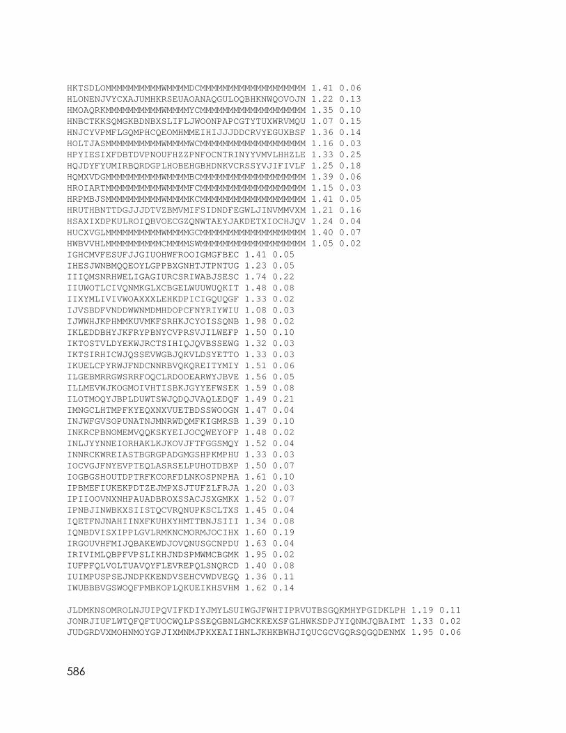
HKTSDLOMMMMMMMMMMWMMMMDCMMMMMMMMMMMMMMMMMMM 1.41 0.06HLONENJVYCXAJUMHKRSEUAOANAQGULOQBHKNWQOVOJN 1.22 0.13HMOAQRKMMMMMMMMMMWMMMMYCMMMMMMMMMMMMMMMMMMM 1.35 0.10HNBCTKKSQMGKBDNBXSLIFLJWOONPAPCGTYTUXWRVMQU 1.07 0.15HNJCYVPMFLGQMPHCQEOMHMMEIHIJJJDDCRVYEGUXBSF 1.36 0.14HOLTJASMMMMMMMMMMWMMMMWCMMMMMMMMMMMMMMMMMMM 1.16 0.03HPYIESIXFDBTDVPNOUFHZZPNFOCNTRINYYVMVLHHZLE 1.33 0.25HQJDYFYUMIRBQRDGPLHOBEHGBHDNKVCRSSYVJIFIVLF 1.25 0.18HQMXVDGMMMMMMMMMMWMMMMBCMMMMMMMMMMMMMMMMMMM 1.39 0.06HROIARTMMMMMMMMMMWMMMMFCMMMMMMMMMMMMMMMMMMM 1.15 0.03HRPMBJSMMMMMMMMMMWMMMMKCMMMMMMMMMMMMMMMMMMM 1.41 0.05HRUTHBNTTDGJJJDTVZBMVMIFSIDNDFEGWLJINVMMVXM 1.21 0.16HSAXIXDPKULROIQBVOECGZQNWTAEYJAKDETXIOCHJQV 1.24 0.04HUCXVGLMMMMMMMMMMWMMMMGCMMMMMMMMMMMMMMMMMMM 1.40 0.07HWBVVHLMMMMMMMMMMCMMMMSWMMMMMMMMMMMMMMMMMMM 1.05 0.02IGHCMVFESUFJJGIUOHWFROOIGMGFBEC 1.41 0.05IHESJWNBMQQEOYLGPPBXGNHTJTPNTUG 1.23 0.05IIIQMSNRHWELIGAGIURCSRIWABJSESC 1.74 0.22IIUWOTLCIVQNMKGLXCBGELWUUWUQKIT 1.48 0.08IIXYMLIVIVWOAXXXLEHKDPICIGQUQGF 1.33 0.02IJVSBDFVNDDWWNMDMHDOPCFNYRIYWIU 1.08 0.03IJWWHJKPHMMKUVMKFSRHKJCYOISSQNB 1.98 0.02IKLEDDBHYJKFRYPBNYCVPRSVJILWEFP 1.50 0.10IKTOSTVLDYEKWJRCTSIHIQJQVBSSEWG 1.32 0.03IKTSIRHICWJQSSEVWGBJQKVLDSYETTO 1.33 0.03IKUELCPYRWJFNDCNNRBVQKQREITYMIY 1.51 0.06ILGEBMRRGWSRRFOQCLRDOOEARWYJBVE 1.56 0.05ILLMEVWJKOGMOIVHTISBKJGYYEFWSEK 1.59 0.08ILOTMOQYJBPLDUWTSWJQDQJVAQLEDQF 1.49 0.21IMNGCLHTMPFKYEQXNXVUETBDSSWOOGN 1.47 0.04INJWFGVSOPUNATNJMNRWDQMFKIGMRSB 1.39 0.10INKRCPBNOMEMVQQKSKYEIJOCQWEYOFP 1.48 0.02INLJYYNNEIORHAKLKJKOVJFTFGGSMQY 1.52 0.04INNRCKWREIASTBGRGPADGMGSHPKMPHU 1.33 0.03IOCVGJFNYEVPTEQLASRSELPUHOTDBXP 1.50 0.07IOGBGSHOUTDPTRFKCORFDLNKOSPNPHA 1.61 0.10IPBMEFIUKEKPDTZEJMPXSJTUFZLFRJA 1.20 0.03IPIIOOVNXNHPAUADBROXSSACJSXGMKX 1.52 0.07IPNBJINWBKXSIISTQCVRQNUPKSCLTXS 1.45 0.04IQETFNJNAHIINXFKUHXYHMTTBNJSIII 1.34 0.08IQNBDVISXIPPLGVLRMKNCMORMJOCIHX 1.60 0.19IRGOUVHFMIJQBAKEWDJOVQNUSGCNPDU 1.63 0.04IRIVIMLQBPFVPSLIKHJNDSPMWMCBGMK 1.95 0.02IUFPFQLVOLTUAVQYFLEVREPQLSNQRCD 1.40 0.08IUIMPUSPSEJNDPKKENDVSEHCVWDVEGQ 1.36 0.11IWUBBBVGSWOQFPMBKOPLQKUEIKHSVHM 1.62 0.14
JLDMKNSOMROLNJUIPQVIFKDIYJMYLSUIWGJFWHTIPRVUTBSGQKMHYPGIDKLPH 1.19 0.11JONRJIUFLWTQFQFTUOCWQLPSSEQGBNLGMCKKEXSFGLHWKSDPJYIQNMJQBAIMT 1.33 0.02JUDGRDVXMOHNMOYGPJIXMNMJPKXEAIIHNLJKHKBWHJIQUCGCVGQRSQGQDENMX 1.95 0.06
586

KFQXCEQYBQSYWDRSDPXYWOOSLJLQQURWRIRMOONBFJJDUQVRJBFRIRCDOODRYIBWPNXSGREJIRQJWDKAOFNLUIPMCAIILSONYUNZDDNRFZ 1.72 0.16
KKWOOHREEEJUQAVCEEBRTVVBVPUJHIUDNQUUNHZDTHDMYPUGJEGUPAJGXNMESDDGCDEMYNCDYINJQQDGYHMRMCPHSVJZPQLTVFFFSWODAS 1.35 0.01
KLPQQUQYSIXVMQDFDAEIDXBLHEQNKPWWSFUIKWRECWGRWNTRKQSNZTQRAQODNEYETSLOBYLSFGGTDWBAYPUOSAYDSPUHJAYTEPVPSYMITP 1.24 0.04
KNVXSIBPKCSPMTCYGJGBKBACKTUEARUPKKHGNUCXUWEMOCLDKTNJYVIHPDQRSDVGHXDRGCTPXUJIHNFFPPNDHFWFIYBINJBTDCIUATHBXG 2.00 0.02
KPUMNHSVGHFQTTXWQLRACVNNRSOROTNEXGQIJMFGPDIJOUYATCHVNHOUBMQCGYJLGPHMBBULJUSPSVRNBKODHHLGXFYUYSANFVFVRTITDE 1.72 0.05
LJSWOSYKITFNRTXIFBSANRCXSEGVINFAFXVHHJJTUHOUIWJTDYOGTXANVIDRAAXUMHHJTJXVLJOFHDIJMJMAIJABSJFIFKAGSEYHSJWSIEARJBSKNKGKVOJHIGFVRFTGOLXANNQVSIIEPXDKBKKCJJLPIRHLJFTKISATMTSJP 1.55 0.13
LJUUKNADVUXNGAFRQDMKIHUDSFRPARHYAGGMEOJWSXOGTRYQTJRFRGDWPQHKQWVVDXMSDHXKAAYFUPVTODYHVTUIRSAOBMLPYQUCWOPFTEGSRAQNWJDHVVRWHDRQRFWXTYLKIULWCBAXKGRDCFREDNPJMNDNMAOJMEOLLNDJM 1.43 0.04
MFFJSKNPJKXDRXXJIJJGLJAAMGNLVJTMPLNHEBDFIEMMHRNVSGIRVTVOIPFMI 1.48 0.14MGRWGVPWQGWJCPIRJWMNTPPPGTQFHNLMLUPPLJVWESGISIHPHRYLXPAWOAPHN 1.54 0.06
MINXSAGQQMMODEJKPNPITOHHGAQNNPJSUMWCQYQHHFPXIJMSFWPWLNWNQVLRH 1.73 0.18MKSOKQDGVGUFHWQYLSFUYFQBDHTBSXEMHOUSNDCJPGIDNKNGPKQLSLDQWPJNQ 1.72 0.05MLQALFYIJMJKKCOBFIVNXFELUGSGBNWHAYWDIQYDRJOUWNLMLOPAKJFBFQHHD 1.69 0.06MLRLDVIRFJRJGILUQYYYSFKHMQQOWRMIIPRGNQJHRKKHYDMXSIYMFPLQRWSSD 1.51 0.04MMACCBHNSGDQNRKVMRDNJWQBFSLRBGBMLPBRKMNMIORGMDMNTHAVXNEHCLPJA 1.76 0.07MMDDKCBROKYJMXXQKPBMJSSMSURNIKSONBTWUCCOPRAGMFPNNTVGRNEQDQYNL 1.57 0.05MMHOQKISLPQJCPKHMRKWOCRJYWDDHCCMOGJRFCIXILWTJQMUXFLCRKNBGQNFX 1.79 0.01MMLIYSWAWFBMXHXQMMWBHKOECJXSHCGMFJSGCGVQFFNBQXMNFMLIRCGTNHSPJ 1.42 0.03MMLOLQBGOTTARNTOMGDQKMUPTBDFTBNMEAWCOWUXLXSIACMNBDWPTMARNKEFN 1.06 0.01MMMNLPBOWPGCVVDNMPQURKHKNXKSVKNMTVMUQLJYKOJFNWMUVCIVGROFBTKNK 1.36 0.02MMMTHIGVYGFFABIQMTDXTWMBDVACEUXMHHBJLSXROGSPJUMCNYFRYMTEWRXOX 1.30 0.02MMOUOUYJTCQPFCPFMXWQCKIWBKFXTMKMCUNEFQEQOGAKEHMODHRGLONHWMCRN 1.36 0.16MMQSQNAJVTXENLDPMEUWPPGVLAIGBWOMWTSAFWOBIKWMYQMGBTOVXDILQKJOE 1.64 0.05MMWYKARXJGXRDLMKKESHNSJEQHJRVEERSWWFXEELSGGMUAOEHWYXLMHNLMLON 1.73 0.01MPGBTHKTSSWCKASIJIUFPXNLESSLJNUNICHOHEETONYWOGJSWMNXHOXEBLFLG 1.71 0.03MQCQGOBGVFLHSXPTPDOOVIREBODHGUMPIYTYPHFWBENBNKOFFBLOLOAPMEHUI 1.85 0.02MQVEIINRFUOYTBNCLVDSANJJXUTTSAWFRMGWDETGAKRMRDVAVSIKBLBUWLCHQ 1.14 0.01MSOJMJRQYAJSCATEFVCPNKHPIKKNKQOIWADJDWGJBJFISJNSBVNPHWYMOGINL 1.47 0.07
NMKAIYSQDHFABDWNQMFPVRJYYVNXPNDGTIOYMTGDIRTAUEXPXITIQPIKUJHOONVEEPICMHUMIDQLBCXFOFCPIACOFYJMICGPJTBAQTRFPAMQMSUNUXTSFHOOMGUNCTEHPTHPCJIAKSKBD 1.85 0.08
NMQJNUVMGQFSHIJOYQCMLIOGXAXUCDXMCPKNMDGFQUKRFBVPKWPBLKTUFEREGFHOYOXRKMAMAYUNAGEECHJDELBJWAGLDINGXIJXEPSGHPMPLFMCGQWAAOLMHYPATAKUYYTPQFIEEITNH 1.580.14
587

QCGPVUQQJPHUYULGKOJNBJEAZPENSZH 1.91 0.02QDPHNYGLPMVYYQOCUIYOLVKFVFIDMIN 1.52 0.01QJFPNELMYBGVUOLEEMJJRICCDKLQMUK 1.80 0.33QJRFPORWBILHPHKQMRUDPUDXIJYGBGF 1.29 0.25
REVUKOGCERMHXEKBCQTJRHCJVXRRIBQAQYHVCXEXIOTVIVKAKKECPWFGPTHXF 1.45 1.99RFTGHODREUPELRRMEVVELSQBHTDDHYYHFQNAFLQRSEAMVAJGPYWYQBUEHFHRF 1.39 0.25RIAFAHLTKWQMGNCDYLEJNEDYULQPHJXKUAMSMDQWKZYDFMVBREESSEGMGOJHK 1.96 1.37RJYQGRWLLATYZGCMHPEZNQNBEDGRLXBSVCZBXHRKLJMERQMCFKTKGKKBLOECH 1.56 1.18RLBVMDKPEEHKIDLRFCJPLXOYTVEUPSTSLNJZLANDNYPWYRGCPGRWNUXTWYRVJ 1.16 0.17RNDZJLUGWZKQUSBPXESCPJZDIJCEDQEBYGCFPNQIKBYDFYHTOPXMKTZLFHNNN 1.24 0.07
RQPXHNHUENPJJOICSJJMEHIEJEDRVVMSTQASROWWMADDPNGXMCMYFCTRXODNA 1.30 0.47RVKNTJDLHNLHODWEIGXXHCCOGAZQIFOFXWJPUUFUQOVYSFENYXJSUNDQESHDL 1.17 0.11RYQAALUJBCNPFEHQWYTQIUSPFGLLCGHDXGAJWWOKENEFCYOVHGXGHQXURHTUC 1.36 0.99
SABKETAXTDIXENYTOTGIFVLULGFOQQJEIYGPAMRRRYBSCXNNXTYDWUIDRBFOGPFMRUUFDRLUFJILAIGYNNSMVHRGEOATODWVLDISWXMMND 1.65 0.22
SDHVJMXJNYTYHPMPGZXFRUCGPONXGAGCVKNORVWCWDFHRJWJWDCBHIEYXJJGAKNRCTJMKMTQEHIJUUPEFAGQHINMBRWDUTYIDWHLJGFFFV 1.41 0.91
SDKUSYQVHCLINLBFHWYDYBYIAAKVIBEUTKGIIHQCENPICOYNWAKJJXOYTYLKVEQMWRAJITCEINHLIYLOWDMHNUHWPWQQJLNMWTLOQLMFUI 1.37 0.43
SFJBUTEWDSLJBIGEASAPGLXTCPQPBNBFMMQJFYECVALMNYGKEVZUMQRKUNUFMBPHUKDKHGJAJKLTTORHEBIFDTQLCMNGGNNJISOBIOJVTL 1.30 0.06
SSAHQOJHWOCLGRCGOGUBHOJRGAVXWQJCSFKLBYWGBBKOKONDNQFQUEASCISKXJWBGINOUMYHRULGSPEATARYGOMQVRUQYKPSNVFTLFADPW 1.19 0.03
SUTYTGVRGAPBEYAVPTRWRNFJSDDMUAVSCIOOXVLDHLOMNCLYGELIMXACINABQQAIKELSKDBHOGWAUPTCTMSBFEWYOPHTOPIXHTUESYNLDU 1.39 0.37
TSTDKLCSQYLOIQFVLHHXTBDGYMGKRJJBZAFDDDUGEKKWUWWVJVPJFTDBSBSNNIIXWMXLMPJELCNGTQHOCWFOYHLHIKZGSGQXSAQJGJJNPUQLKPCEQQWFKVQQOPSLYGPRWUQICYUFQIQWKBVGKRZCDTRSDMOQMENFDIXATYCBH 1.88 3.85
UBLFBKKFNATJVTJUKJFGALBIPQHVRUMAROTNVHBLAQVSHVHRGLFJAAABFRJFW 1.81 0.07UKDGJLEXISFBNTDVQVMXQFXCGMQKOSUHDOFPYOOECJEEOPMNLSQCPEYJEYIGO 1.10 0.16ULYMXJCIVBIBCHWVWSEEKQVKQIOJBQHQSHJOFBPPDWSMBTVSERGGYPPPATWSB 1.52 0.13UMALDKMYNVYSDIAQVVHAWOJGDLFHKPSQEDJWPSOQCBFHGYMIVIXGXYCITMAXH 1.33 0.10
VBDIYXAGPEUVXXPCKVYCLPPRBAYDQTEIRDGMWBDIHIJAPGSLDYDLMTANMNMHNCLTYBJGXAYBJBLFJXDJRKOHCNPBIRTSLGSYSDOLUNAQTIJMNVOEIUOKAHLIXWPEMPQQFTMVPUFECMACT 1.69 0.60
VHETJPMKNMHQNUVBIOTFADJUXXIQRSGDSNXAGNEKPMCJRIDEHOFTVTPLWUFLNDCWLKHXKKELUMBDOHSIBSDEWWSPLQVMWLQERMCANDUBCXULQWYGOTLGLLQFSJGVQEUIEQQXXWGEKVTPA 1.03 0.14
VMMKMRMREPCPYAFRGJBOTPHNQRFXVNSNYQVJNBXXPKRPVHFQAF
588

GFSTHYFKCIDWXOQJAKRFKHPYHNENTDQLJMQGMXTFPBDFUIPAIODWYAMTXJDIWGERTHDOKWFXPLSWFYPXNQMNOBKILSG 1.84 0.44
YAMHDWIODTE 1.49 0.09YAQCXBTDRHF 1.43 0.36YBJSRTYCQLD 1.50 0.22YDNBSGGTQDW 1.39 0.15YEBYSXDGLVB 1.54 0.42YELRVNTLOBU 1.34 0.21YHKTEILDYRK 1.20 0.01YLNVRNDFOTX 1.30 0.12YOJMOEAKWYV 1.00 0.02YSMLSCXTGBR 1.20 0.03YVBTGBLJNUB 1.42 0.41YWOABOXTDFD 1.48 0.32ZAMWBPMDUAXGGLB 1.47 0.13ZBBCMQDQKTJPSUR 1.15 0.02ZCBINUXAKUFLEAK 1.59 0.06ZCTFTHMKITVNFFG 1.69 0.08ZEIVGPLCKGALTXT 1.41 0.01ZFPEIBFLSVWGFPA 1.09 0.01ZKRFMRHHAVUOIKM 1.16 0.02ZLFBPYYLFUKMSED 1.18 0.01ZMEROSWMYGDQTKO 1.87 0.01ZMIVEQTDVEEOWVN 1.70 0.03ZNFEMVRCISEHSIN 1.28 0.03ZNVIDLJDFUUQUBK 1.04 0.03ZOCGMCVDMPDFMHJ 1.64 0.06ZRLDWMOJKXHBLAN 1.73 0.03ZSVGLBHQEXQQMEE 1.21 0.01[IAWNTNHKJOCOSY 1.32 0.33[JJMLWFVTUKDTTQ 1.97 0.20\ASEFAHYBJUVPHIMWYT 1.54 0.27\BBTXCFCJUGDJXKONUH 1.56 0.12\IUPGKKXXOTAUMPEPDN 1.30 0.29\JISPFOVANDEBNXUWBY 1.48 0.21\JJIASHWXGPXCGROCWG 1.36 0.17\KBDABMSIBRWMQNMUKW 1.69 0.21\LLXGLCOXAJDQJOICVC 1.70 0.10\MEOANCSXDVGCVLGHQT 1.65 0.10\NBIAYCYGUSVJFXEJGA 1.32 0.29\NGPKOPDSBDCBGVBBPP 1.58 0.12\SCNPBHGXICIDBPKQSI 1.48 0.20\TOFXBCFVQIXXQUWDXB 1.41 0.19\TTKFATYUYRXVWLWHQB 1.06 0.19]CDUHTE 1.10 0.04]FDDLCE 1.06 0.03]HDFNTE 1.20 0.03]HGEWRK 1.17 0.02]KFUDSM 1.21 0.02]KSFJWS 1.02 0.01
589
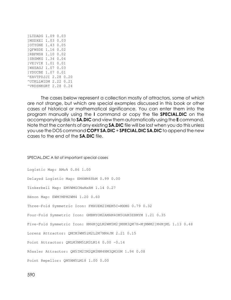
]LTDADG 1.09 0.03]MSDXEI 1.03 0.03]OTYGNE 1.43 0.05]QFWSDE 1.16 0.02]RBFMSH 1.10 0.02]SBSMKG 1.34 0.04]VEIVIK 1.01 0.01]WXSAGJ 1.07 0.03]YDUCBE 1.07 0.01^EAVTPDJJI 2.28 0.20^UTKLLWIDM 2.22 0.21^VRDSNKGRT 2.28 0.24
The cases below represent a collection mostly of attractors, some of whichare not strange, but which are special examples discussed in this book or othercases of historical or mathematical significance. You can enter them into theprogram manually using the I command or copy the file SPECIAL.DIC on theaccompanying disk to SA.DIC and view them automatically using the E command.Note that the contents of any existing SA.DIC file will be lost when you do this unlessyou use the DOS command COPY SA.DIC + SPECIAL.DIC SA.DIC to append the newcases to the end of the SA.DIC file.
SPECIAL.DIC A list of important special cases
Logistic Map: AMu% 0.86 1.00
Delayed Logistic Map: EM4WM48bM 0.99 0.00
Tinkerbell Map: EMVWMGCMaMaRM 1.14 0.27
Hénon Map: EWM?MPM2WM4 1.20 0.60
Three-Fold Symmetric Icon: FMXUEM2IMEM5C=MXMG 0.79 0.32
Four-Fold Symmetric Icon: GMBMYOM2AMAM4OM5UAM3EBMYM 1.21 0.35
Five-Fold Symmetric Icon: HM4MjQLM2WM5M2jMHM3QM7H=MjMWM2]M4MjML 1.13 0.48
Lorenz Attractor: QMCM3WM5iM2L2M7NM4JM 2.21 0.15
Point Attractor: QMLM3NM5LM3LM14 0.00 -0.14
Rössler Attractor: QM5IM2IM2QM3NM4NM3QM30M 1.94 0.08
Point Repellor: QM5NM5LM18 1.00 0.00
590

Van der Pol Equation: RM11OM9KM2KM6OM28 1.04 0.00
Symmetric Limit Cycle: RMNMAM3AM3NM9LM2AM6NMAM26 1.04 0.00
2-Torus: VMNMAM4AM7NM19LM2AM11NMAM42NMAM2AOM28LM2AM2NMA 1.04 0.00
2-Torus (rotated): VMNMAM8AM13NM24NMAM6AM6OM3LM3AM20NMAM22LM3AM11NMA 1.04 0.00
Gingerbread Man: YCMC2M2WM3 1.42 0.11
Tent Map: YM2WM2VM39 1.23 1.00
Lozi Attractor: YWMW<M2RM3 1.67 0.68
Chirikov (Standard) Map: \MWM4dWqMW2M3dWq 1.13 0.04
Circle Map: \NWMyWM4NM2yWM4 1.16 1.28
Birkhoff's Bagel: ^BVKBDVHIK 1.90 0.22
Forced Damped Hard Spring: ^WCLM2KMWJ 1.01 -0.01
Forced Van der Pol Oscillator: ^WCMCMWMSD 1.68 0.00
Forced Damped Linear Spring: ^WCM3KMWJ 0.92 -0.07
Forced Damped Soft Spring: ^WCNM2JMWJ 1.01 -0.20
Duffing Two-Well Oscillator: ^W2CM2KMRD 2.84 0.15
591


![Detecting strange attractors in turbulenceDetecting strange attractors in turbulence. Floris Takens. 1. Introduction. Since [19] was written, much more accurate experiments on the](https://static.fdocuments.us/doc/165x107/610aaef3c2c6872ad446fca5/detecting-strange-attractors-in-detecting-strange-attractors-in-turbulence-floris.jpg)