Story of IBM Research’s success at KDD/Netflix Cup 2007
26
© Copyright IBM Corporation 2007 Story of IBM Research’s success at KDD/Netflix Cup 2007 Saharon Rosset TAU Statistics (Formerly IBM) IBM Research’s teams: Task 1: Yan Liu, Zhenzhen Kou (CMU intern) Task 2: Saharon Rosset, Claudia Perlich, Yan Liu
-
Upload
carmelita-aguilar -
Category
Documents
-
view
29 -
download
0
description
Story of IBM Research’s success at KDD/Netflix Cup 2007. Saharon Rosset TAU Statistics (Formerly IBM) IBM Research’s teams: Task 1: Yan Liu, Zhenzhen Kou (CMU intern) Task 2: Saharon Rosset, Claudia Perlich, Yan Liu. October 2006 Announcement of the NETFLIX Competition. USAToday headline: - PowerPoint PPT Presentation
Transcript of Story of IBM Research’s success at KDD/Netflix Cup 2007

© Copyright IBM Corporation 2007
Story of IBM Research’s success atKDD/Netflix Cup 2007
Saharon RossetTAU Statistics (Formerly IBM)
IBM Research’s teams:Task 1: Yan Liu, Zhenzhen Kou (CMU intern) Task 2: Saharon Rosset, Claudia Perlich, Yan Liu
IBM Research – Mathematical Sciences Department
© Copyright IBM Corporation 2007Slide 2
IBM Research – Mathematical Sciences Department
© Copyright IBM Corporation 2007Slide 3
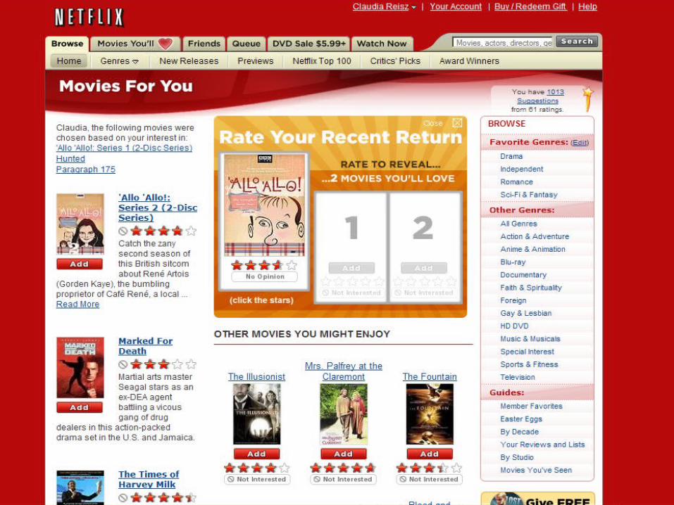
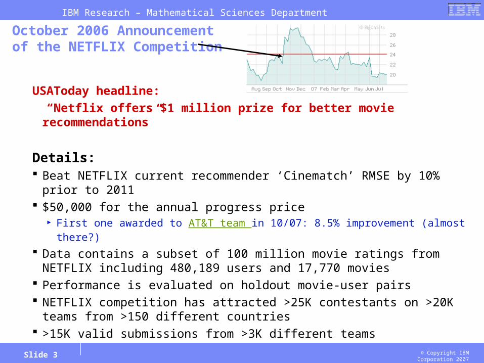
October 2006 Announcement of the NETFLIX Competition
USAToday headline:
“Netflix offers $1 million prize for better movie recommendations”
Details: Beat NETFLIX current recommender ‘Cinematch’ RMSE by 10% prior to 2011 $50,000 for the annual progress price
First one awarded to AT&T team in 10/07: 8.5% improvement (almost there?)
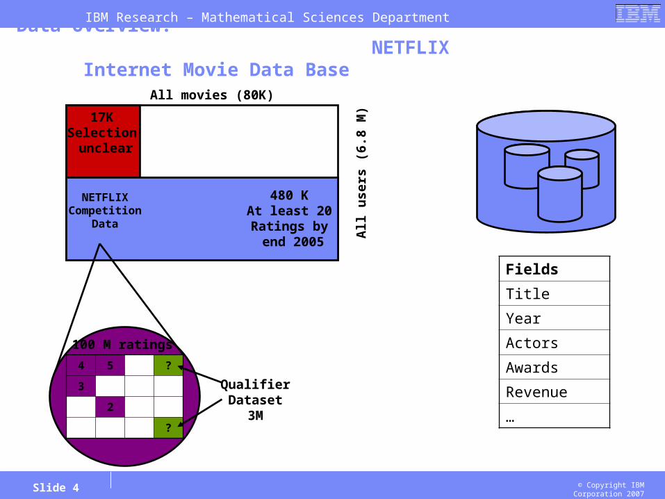
Data contains a subset of 100 million movie ratings from NETFLIX including 480,189 users and 17,770 movies
Performance is evaluated on holdout movie-user pairs NETFLIX competition has attracted >25K contestants on >20K teams from >150
different countries >15K valid submissions from >3K different teams
IBM Research – Mathematical Sciences Department
© Copyright IBM Corporation 2007Slide 4
All movies (80K)
All
use
rs (
6.8
M)
NETFLIXCompetition
Data
17KSelection unclear
480 KAt least 20Ratings by end 2005
100 M ratings
Data Overview: NETFLIX Internet Movie Data Base
Fields
Title
Year
Actors
Awards
Revenue
…
4 5 ?
3
2
?
QualifierDataset
3M

IBM Research – Mathematical Sciences Department
© Copyright IBM Corporation 2007Slide 5
17K
mo
vie
s
Training Data Task 2
Task 1 Movie Arrival
1998 Time 2005 2006
User Arrival
4 5 ?
3
2
?
QualifierDataset
3M
KDD CUP
NO Useror MovieArrival
NETFLIX data generation process
IBM Research – Mathematical Sciences Department
© Copyright IBM Corporation 2007Slide 6
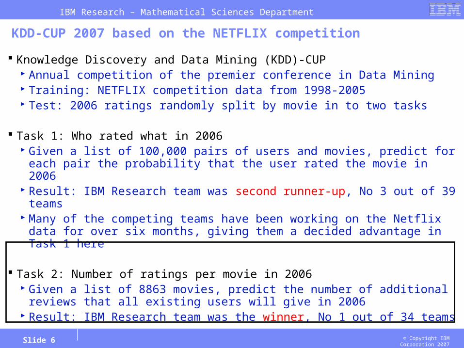
KDD-CUP 2007 based on the NETFLIX competition
Knowledge Discovery and Data Mining (KDD)-CUP Annual competition of the premier conference in Data Mining Training: NETFLIX competition data from 1998-2005 Test: 2006 ratings randomly split by movie in to two tasks
Task 1: Who rated what in 2006 Given a list of 100,000 pairs of users and movies, predict for each pair the
probability that the user rated the movie in 2006 Result: IBM Research team was second runner-up, No 3 out of 39 teams Many of the competing teams have been working on the Netflix data for
over six months, giving them a decided advantage in Task 1 here
Task 2: Number of ratings per movie in 2006 Given a list of 8863 movies, predict the number of additional reviews that
all existing users will give in 2006 Result: IBM Research team was the winner, No 1 out of 34 teams

IBM Research – Mathematical Sciences Department
© Copyright IBM Corporation 2007Slide 7
Generation of Test sets from 2006 for Task 1 and Task 2
Task 1
Task 2
Users
Mo
vies
183
8
24
316
19324
89
25
375
0
RatingTotals
2.2
0.9
1.4
2.5
4.2
1.9
1.4
2.6
0log(n+1)
Marginal 2006Distribution of
rating
Movie User Rating
M1 U31 4
M832 U83
M63 U2 3
M83 U97
M527 U63 1
M36 U81
… … …
Task 2Test Set (8.8K)
Remove Pairs that were
rated prior to 2006
Movie User Rating
M1 U31 1
M832 U83 0
M63 U2 1
M83 U97 0
M527 U63 0
… … …
Task 1Test Set (100K)
Sample (movie, user)
pairs according to product of
marginals
Back

IBM Research – Mathematical Sciences Department
© Copyright IBM Corporation 2007Slide 8
Insights from the battlefields: What makes a model successful?
Components of successful modeling:
1. Data and domain understanding• Generation of data and task• Cleaning and representation/transformation
2. Statistical insights• Statistical properties• Test validity of assumptions• Performance measure
3. Modeling and learning approach• Most “publishable” part• Choice or development of most suitable algorithm
Imp
ort
an
ce?

IBM Research – Mathematical Sciences Department
© Copyright IBM Corporation 2007Slide 9
Task 1: Did User A review Movie B in 2006?
Task formulation A classification task to answer question whether “existing” users will
review “existing” movies
Challenges Huge amount of data
• how to sample the data so that any learning algorithms can be applied is critical
Complex affecting factors• decrease of interest in old movies, growing tendency of watching (reviewing) more
movies by Netflix users
Key solutions Effective sampling strategies to keep as much information as possible Careful feature extraction from multiple sources

IBM Research – Mathematical Sciences Department
© Copyright IBM Corporation 2007Slide 10
Task 1: Effective Sampling Strategies
Sampling the movie-user pairs for “existing” users and “existing” movies from 2004, 2005 as training set and 4Q 2005 as developing set The probability of picking a movie was proportional to the number of ratings that movie
received; the same strategy for users
……
Movie5 .0011 ……
Movie3 .001……
Movie4 .0007
……
User7 .0007 ……
User6 .00012……
User8 .00003……
Movies
Users
……
Movie5 User 7 ……
Movie3 User 7……
Movie4 .User 8
….1488844,3,2005-09-06822109,5,2005-05-13885013,4,2005-10-1930878,4,2005-12-26823519,3,2004-05-03
…
HistorySamples

IBM Research – Mathematical Sciences Department
© Copyright IBM Corporation 2007Slide 11
Task 1: Effective Sampling Strategies
Sampling the movie-user pairs for “existing” users and “existing” movies from 2004, 2005 as training set and 4Q 2005 as developing set The probability of picking a movie was proportional to the number of ratings that movie
received; the same strategy for users
……
Movie5 .0011 ……
Movie3 .001……
Movie4 .0007
……
User7 .0007 ……
User6 .00012……
User8 .00003……
Movies
Users
……
Movie5 User 7 ……
Movie3 User 7……
Movie4 .User 8
The Ratio of Positive Examples
IBM Research – Mathematical Sciences Department
© Copyright IBM Corporation 2007Slide 12
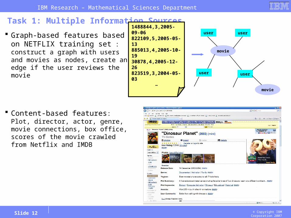
Task 1: Multiple Information Sources
Graph-based features based on NETFLIX training set : construct a graph with users and movies as nodes, create an edge if the user reviews the movie
Content-based features: Plot, director, actor, genre, movie connections, box office, scores of the movie crawled from Netflix and IMDB
1488844,3,2005-09-06822109,5,2005-05-13885013,4,2005-10-1930878,4,2005-12-26823519,3,2004-05-03
…
movie
useruser
movie
user user

IBM Research – Mathematical Sciences Department
© Copyright IBM Corporation 2007Slide 13
Task 1: Feature Extraction
Movie-based features• Graph topology: # of ratings per movie (across different years), adjacent scores between movies
calculated using SVD on the graph matrix
• Movie content: similarity of two movies calculated using Latent Semantic Indexing based on bag of words from (1) plots of the movie and (2) other information, such as director, actors, and genre
User profile• Graph topology: # of ratings per user (across different years)
• User preferences based on the movies being rated: key word match count, average/min/max of similarity scores between the movie being predicted and movies having been rated by the user
movie (rated)
user
movie (rated)
movie (rated)
…
movie (to predict)
key word match count, average/min/max of similarity scores

IBM Research – Mathematical Sciences Department
© Copyright IBM Corporation 2007Slide 14
Task 1: Learning strategy
Learning Algorithm: Single classifiers: logistic regression, Ridge regression, decision tree, support vector
machines Naïve Ensemble: combining sub-classifiers built on different types of features with pre-set
weights Ensemble classifiers: combining sub-classifiers with weights learned from the development
set

IBM Research – Mathematical Sciences Department
© Copyright IBM Corporation 2007Slide 15
Task 2 description: How many reviews did a Movie receive in 2006?
Task formulation Regression task to predict the total count of reviewers from “existing”
users for 8863 “existing” movies
Challenges Movie dynamics and life-cycle
• Interest in movies changes over time
User dynamics and life-cycle• No new users are added to the database
Key solutions Use counts from test set of Task 1 to learn a model for 2006 adjusting for pair
removal Build set of quarterly lagged models to determine the overall scalar Use Poisson regression
IBM Research – Mathematical Sciences Department
© Copyright IBM Corporation 2007Slide 16
Some data observations
1. Task 1 test set is a potential response for training a model for Task 2 Was sampled according to marginal
(= # reviews for movie in 06 / total # reviews in 06)which is proportional to the Task 2 response (= # reviews for movie in 06)
BIG advantage: we get a view of 2006 behavior for half the movies Build model on this half, apply to the other half (Task 2 test set)
Caveats:• Proportional sampling implies there is a scaling parameter left, which we don’t
know• Recall that after sampling, (movie, person) pairs that appeared before 2006 were
dropped from Task 1 test set Correcting it is an inverse rejection sampling problem
2. No new movies and reviewers in 2006 Need to emphasize modeling the life-cycle of movies (and reviewers)
• How are older movies reviewed relative to newer movies?• Does this depend on other features (like movie’s genre)?
This is especially critical when we consider the scaling caveat above

IBM Research – Mathematical Sciences Department
© Copyright IBM Corporation 2007Slide 17
Some statistical perspectives
1. Poisson distribution is very appropriate for counts Clearly true of overall counts for 2006
• Assuming any kind of reasonable reviewers arrival process• Implies appropriate modeling approach for true counts is Poisson regression:
ni ~ Pois (it)log(i) = j j xij
* = arg max l(n ; X,) (maximum likelihood solution)
What happens when we sub-sample for Task 1 test set?• Sum is fixed multinomial• This makes no difference in terms of modeling, since Poisson regression always
preserves the sum What does this imply for model evaluation approach?
• Variance stabilizing transformation for Poisson is square root ni has roughly constant variance RMSE of log (prediction +1) against log(# ratings +1) emphasizes performance on unpopular movies (small Poisson parameter larger log scale variance)
• We still assumed that if we do well in a likelihood formulation, we will do well with any evaluation approach

IBM Research – Mathematical Sciences Department
© Copyright IBM Corporation 2007Slide 18
2. Can we invert the rejection sampling mechanism? This can be viewed as a missing data problem
• Where:- ni, mj are the counts for movie i and reviewer j respectively
- pi, qj are the true marginals for movie i and reviewer j respectively
- N is the total number of pairs rejected due to review prior to 2006
- Ui, Pj are the users who reviewed movie i prior to 2006 and movies reviewed by user j prior to 2006, respectively
• Can we design a practical EM algorithm with our huge data size? Interesting research problem…
We implemented ad-hoc inversion algorithm• Iterate until convergence between:
- assuming movie marginals are correct and adjusting reviewer marginals- assuming reviewer marginals are correct and adjusting movie marginals
We verified that it indeed improved our data since it increased correlation with 4Q2005 counts
Some statistical perspectives (ctd.)
j
i
Piijj
Ujjii
pNqqpNmE
qNpqpNnE
)1)(100000(),,|(
)1)(100000(),,|(
IBM Research – Mathematical Sciences Department
© Copyright IBM Corporation 2007Slide 19
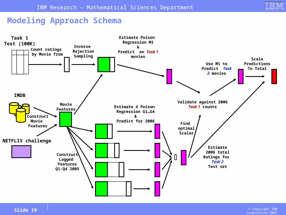
Modeling Approach Schema
Inverse RejectionSampling
Count ratings by Movie from
Estimate Poison Regression M1
&Predict on Task 1
movies
Task 1Test (100K)
MovieFeatures
IMDB
ConstructMovie
Features
ConstructLagged Features
Q1-Q4 2005
Validate against 2006Task 1 counts
NETFLIX challenge
Estimate 4 Poison Regression G1…G4
&Predict for 2006
Find optimalScalar
Estimate2006 total
Ratings for Task 2
Test set
Use M1 toPredict Task 2
movies
ScalePredictions
To Total

IBM Research – Mathematical Sciences Department
© Copyright IBM Corporation 2007Slide 20
Some observations on modeling approach
1. Lagged datasets are meant to simulate forward prediction to 2006 Select quarter (e.g., Q105), remove all movies & reviewers that “started” later Build model on this data with e.g., Q305 as response Apply model to our full dataset, which is naturally cropped at Q405
Gives a prediction for Q206 With several models like this, predict all of 2006 Two potential uses:
• Use as our prediction for 2006 – but only if better than the model built on Task 1 movies!
• Consider only sum of their predictions to use for scaling the Task 1 model
2. We evaluated models on Task 1 test set Used holdout when also building them on this set How can we evaluate the models built on lagged datasets?
• Missing a scaling parameter between the 2006 prediction and sampled set• Solution: select optimal scaling based on Task 1 test set performance
Since other model was still better, we knew we should use it!

IBM Research – Mathematical Sciences Department
© Copyright IBM Corporation 2007Slide 21
Some details on our models and submission
All models at movie level. Features we used: Historical reviews in previous months/quarters/years (on log scale) Movie’s age since premier, movie’s age in Netflix (since first review)
• Also consider log, square etc have flexibility in form of functional dependence Movie’s genre
• Include interactions between genre and age “life cycle” seems to differ by genre!
Models we considered (MSE on log-scale on Task 1 holdout): Poisson regression on Task 1 test set (0.24) Log-scale linear regression model on Task 1 test set (0.25) Sum of lagged models on built on 2005 quarters + best scaling (0.31)
Scaling based on lagged models Our estimated of number of reviews for all models in Task 1 test set: about
9.5M• Implied scaling parameter for predictions about 90• Total of our submitted predictions for Task 2 test set was 9.3M
IBM Research – Mathematical Sciences Department
© Copyright IBM Corporation 2007Slide 22
Competition evaluation
First we were informed that we won with RMSE of ~770 They mistakenly evaluated on non-log scale Strong emphasis on most popular movies We won by large margin
Our model did well on most popular movies!
Then they re-evaluated on log scale, we still won On log scale the least popular movies are emphasized
• Recall that variance stabilizing transformation is in-between (square root) So our predictions did well on unpopular movies too!
Interesting question: would we win on square root scale (or similarly, Poisson likelihood-based evaluation)? Sure hope so!

IBM Research – Mathematical Sciences Department
© Copyright IBM Corporation 2007Slide 23
Competition evaluation (ctd.)
Results of competition (log-scale evaluation):
Components of our model’s MSE: The error of the model for the scaled-down Task 1 test set (which we
estimated at about 0.24) Additional error from incorrect scaling factor
Scaling numbers: True total reviews: 8.7M Sum of our predictions: 9.3M
Interesting question: what would be best scaling For log-scale evaluation? Conjecture: need to under-estimate true total For square-root evaluation? Conjecture: need to estimate about right

IBM Research – Mathematical Sciences Department
© Copyright IBM Corporation 2007Slide 24
Effect of scaling on the two evaluation approaches
ScalingTotal reviews
(M)Log-scale
MSESquare-root scale
MSE Comment
0.7 6.55 0.222 40.28
0.8 7.48 0.208 29.80 Best log performance
0.9 8.42 0.225 26.38Best sqrt performance
0.93 8.70 0.234 26.55 Correct scaling
1 9.35 0.263 28.86 Our solution
1.1 10.29 0.316 36.37

IBM Research – Mathematical Sciences Department
© Copyright IBM Corporation 2007Slide 25
7 8 9 10
0.2
00
.22
0.2
40
.26
0.2
80
.30
25
28
31
34
37
40
0.2
00
.22
0.2
40
.26
0.2
80
.30
Legend
Log-scale MSE
SQRT MSE
True sum
Submitted sum
Sum predictions (M)
Effect of scaling on the two evaluation approaches

IBM Research – Mathematical Sciences Department
© Copyright IBM Corporation 2007Slide 26
Acknowledgements
Claudia Perlich Yan Liu Rick Lawrence And many more ..