Storm Track Variations As Seen in Radiosonde Observations ...

480 VOLUME 16J O U R N A L O F C L I M A T E

q 2003 American Meteorological Society

Storm Track Variations As Seen in Radiosonde Observations and Reanalysis Data

NILI HARNIK

Lamont-Doherty Earth Observatory, Palisades, New York

EDMUND K. M. CHANG

ITPA/MSRC, State University of New York at Stony Brook, Stony Brook, New York

(Manuscript received 14 December 2001, in final form 18 July 2002)

ABSTRACT

The interannual variations in the Northern Hemisphere storm tracks during 1949–99 based on unassimilated ra-diosonde data are examined and compared to similarly derived quantities using the NCEP–NCAR reanalysis at sondetimes and locations. This is done with the motivation of determining the extent to which the storm track variationsin reanalysis data are real. Emphasis is placed on assessing previous findings, based on NCEP–NCAR reanalysis data,that both storm tracks intensified from the 1960s to the 1990s with much of the intensification occurring during theearly 1970s, and that the Atlantic and Pacific storm tracks are significantly correlated.

Sonde data suggest that the Atlantic storm track intensified during the 1960s to 1990s, but the intensificationwas weaker than the reanalysis suggests. The larger trend in reanalysis is due to an overall decrease in biaseswith time. In the Pacific storm track entrance and exit regions, sonde data show notable decadal timescaleoscillations, similar to the reanalysis, but no significant overall positive trend. Sonde data does show a positivetrend over Canada, consistent with a Pacific storm track intensification and northeastward shift, but lack of dataover the storm track peak prevents drawing any strong conclusions. The biases in the reanalysis are found tohave a strong spatial pattern, with the largest biases being over the Pacific entrance region (Japan).

The correlation between the Atlantic and Pacific storm tracks in sonde data (which exists mainly over thestorm track entrance and exit regions) is not as significant as in the reanalysis, with differences being mostlydue to the decadal timescale variations of the storm tracks rather than their year-to-year variations.

1. Introduction and motivation

The midlatitude storm tracks are the locations wherebaroclinic cyclones prevail. There are two popular waysto define the storm tracks. The first methodology takesa synoptic view and defines storm tracks based on cy-clone count statistics (e.g., Petterssen 1956; Whitakerand Horn 1984). This certainly makes sense since thesecyclones are the systems that significantly impact theweather of the regions over which they pass through,especially during the cool seasons. An alternative def-inition takes the storm tracks to be regions where tran-sient eddy variance/covariance statistics are maximal(e.g., Blackmon 1976; Lau 1978). Such a definition isbased on the fact that these cyclones are associated withdeep baroclinic waves that transport heat, moisture, andmomentum which significantly impact the planetaryscale flow field (for a review, see Chang et al. 2002).While these two definitions are not necessarily congru-ent (Wallace et al. 1988; Paciorek et al. 2002), in theNorthern Hemisphere they both pick out the midlatitude

Corresponding author address: Nili Harnik, Lamont-Doherty EarthObservatory, 61 Route 9W, Palisades, NY 10964.E-mail: [email protected]

regions over the oceanic basins to be the most prominentregions. Here, storm tracks will be defined based oneddy variance statistics.

In this paper we compare the storm track variationscomputed based on the National Centers for Environ-mental Prediction–National Center of Atmospheric Re-search (NCEP–NCAR) reanalysis dataset (Kalnay et al.1996; Kistler et al. 2001) to those computed using ob-servations based on the unassimilated radiosonde data,in order to determine whether the decadal timescale var-iations of the intensity of the storm tracks, observed inreanalysis data, are real.

In particular, we want to verify recent results of Changand Fu (2002, hereafter CF), who showed that both thePacific and Atlantic storm tracks intensified by nearly40% from the 1960s to the late 1980s and early 1990s.Based on the reanalysis data, the leading empirical or-thogonal function (EOF) of the storm tracks (defined asthe variance of high-pass-filtered meridional velocityperturbation at 300-hPa level) is found to be a mutualintensification of the Pacific and Atlantic storm tracks,and the corresponding principal component (PC) timeseries shows a transition from weak storm tracks before1971 to stronger storm tracks after 1975. Chang and Fu

1 FEBRUARY 2003 481H A R N I K A N D C H A N G

(2002) also showed a significant correlation between theindividual Atlantic and Pacific storm-track PCs, evenon a month-to-month basis, suggesting the mutual in-tensification is not an artifact of the EOF analysis butrather that the two storm tracks vary to some extenttogether.

The need for a verification of CF’s results using sondedata arises because there may be biases in the reanalysisthat affect the observed variations in the storm tracks.These biases can arise for the following reasons: ob-servations are sparse or nonexistent near the peaks ofthe storm tracks, hence they do not constrain the re-analysis very strongly (e.g., Chang 2000, showed thatthe storm track intensity over the Southern Hemisphere,where observations are sparse, differs significantly be-tween the NCEP–NCAR and European Centre for Me-dium-Range Weather Forecasts (ECMWF) reanalyses);while the reanalysis minimizes the rms difference fromsonde observations, the intensity of the storm tracks ismeasured by eddy variance, which is not necessarilyoptimally analyzed (see appendix A); large changes insonde and aircraft measurement coverage over the yearsmight introduce large biases in the analysis (Ebisuzakiand Kistler 1999; Kistler et al. 2001).

Several other studies also suggested that there has beena secular trend in the Northern Hemisphere storm trackactivity. Based largely on cyclone counts statistics com-puted from the NCEP–NCAR reanalysis data, Geng andSugi (2001) suggested that the cyclone activity over thenorthern North Atlantic, in terms of cyclone density, cy-clone deepening rate, as well as cyclone central pressuregradient, all exhibit a significant intensifying trend alongwith a decadal timescale oscillation in winter during thepast 40 yr. Meanwhile, Graham and Diaz (2001) suggestedthat the frequency and intensity of extreme cyclones overthe North Pacific Ocean over the past 50 years has in-creased markedly. In addition, Paciorek et al. (2002) alsofound an increase in the number of intense cyclones overboth oceanic regions. On the other hand, Gulev et al.(2001), using a somewhat different cyclone tracking tech-nique, found a significant decrease in the number of cy-clones over the Pacific, with no significant trend in thenumber of intense cyclones over the sector, and significantdecrease in both the number of cyclones and intense cy-clones over the Atlantic sector, though the number of in-tense cyclones are found to have increased in the Arctic.However, their results did suggest an increase in the av-erage intensity and deepening rates of cyclones. Whatleads to the discrepancies between the results of Gulev etal. and those of the other groups is not entirely clear, butit could be due to differences in the tracking routines [seethe appendix in Gulev et al. (2001)], differences in thedefinition of cyclone frequencies and intense cyclones,and/or differences in the geographical extent of the av-eraging areas.

While it is not clear how the eddy variance and co-variance statistics relate to cyclone counts, we expectthat any biases in eddy variances could also show up

as biases in cyclone intensity and thus could also affectcyclone statistics based on counts of intense cyclones.The results of Graham and Diaz (2001), Geng and Sugi(2001), and Gulev et al. (2001) are based largely onNCEP–NCAR reanalysis data, though Graham and Diaz(2001) did provide supplementary support by compar-ison with some in situ observations. Clearly, more com-parisons need to be made between NCEP–NCAR re-analysis data and unassimilated observations to verifythe trend displayed in the reanalysis dataset.

Chang and Fu (2002) analyzed data from 21 sondestations along the storm tracks. They found evidencefor the intensification of the storm tracks, but weaker,suggesting there could be some biases in the reanalysisdata that changed with time. In this paper we comparethe interannual variations of the storm tracks in sondeand reanalysis data, using all sonde observations thatwent into the reanalysis between 1949 and 1999. UsingEOF analysis we also examine whether the mutual var-iation of the two storm tracks, and the transition froma weak to strong storm track in the early 1970s, arefound in sonde data.

2. Data and diagnostics

We use archived NCEP–NCAR radiosonde data fromall stations that reported during 1949–99, in the latituderange of 208–808N. The dataset includes ship reports andland stations. The observational data archive was producedas part of the reanalysis project (Kistler et al. 2001).

To diagnose storm track strength, we use the 300-hPameridional winds variance, computed using a 24-h dif-ference filter (Wallace et al. 1988), denoted by V1df, andcalculated as follows:

2V 5 [V 2 V ] , (1)1df (t124 h) (t)

where the overbar denotes an average over all availableobservation times. Chang and Fu (2002) showed that thismeasure of storm track strength is comparable to morecommon diagnostics. We use it because it can easily beapplied to time series with observation gaps. We presentresults for winter mean [December–February (DJF)] sta-tistics, and note that calculations using January data givesimilar results. We denote each winter by the correspond-ing January year (meaning our dataset starts December1948).

Most stations report every 12 h, some report every6 h, and occasionally a station report contains missingor bad data, which is flagged in the raw dataset. Wefilter out obviously bad sonde reports, that exceed 80m s21 and differ from the corresponding reanlysis grid-point value by more than 30 m s21. Only a tiny percentof the observations are filtered, and most of these areclearly bogus reports of winds much stronger than 100m s21. Similar calculations with different filtering limits,give similar results.

The NCEP–NCAR reanalysis pressure level datasetcomprises 6-hourly data on a 2.58 3 2.58 grid. For com-


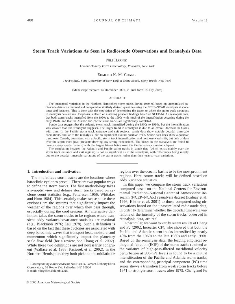
FIG. 1. (top) The number of years with observations (colored rectangles) plotted at the observation location,and the reanalysis 1949–99 mean V1df (contours). (bottom) The averaging areas used in this study (see textfor details) and grids with more than 25 yr of SONDE observations (maroon dots).

parison, we compile a gridded sonde dataset (SONDE)as follows. For each reanalysis grid box we search thesonde dataset for all stations that are located within it.Most of the grid boxes that contain an observing stationhave only one. When there are more than one stationin a grid box, we use data from the station with thelargest number of valid reports during the month, andfill in data gaps using other stations. We also repeated

some of the calculations using an average of all reportsin a grid box and found only tiny differences.

We only use winter statistics for stations that reportedvalid meridional winds more than half the time (90 re-ports in DJF, assuming 12-h reports) and more than aquarter of the time during individual months (more than15 reports during December and January, and more than14 reports during February). This threshold is reason-


FIG. 2. The decadal means of V1df for (top) the high (1990–99) and (bottom) low (1962–71) decades forSONDE (colored rectangles) and the full reanalysis data (contours). SONDE data are shown only for gridsthat have at least 25 yr of observations. To facilitate comparison, the same color scheme is used for thereanalysis contours and SONDE rectangles.

able in comparison with other studies using sonde data(Kidson and Trenberth 1988). Figure 1 (top) shows thenumber of years of sufficient sonde observations foreach grid box, superposed over the mean storm trackstrength (1949–99 mean of V1df). We see that there isvery little coverage (temporal and spatial) over the peaksof the storm tracks, in particular, the Pacific one. Ourresults, therefore, are based on the storm track entranceand exit regions, which do have a decent coverage.

For direct comparison with the reanalysis, we repeatour calculations using the reanalysis data only at gridpoints and synoptic times that have SONDE data. Werefer to this sampled reanalysis dataset as RSAMP.

3. Results

In the following section we examine the variabilityof the storm tracks as seen in two kinds of analyses,one based on the full datasets (section 3a), and the otherbased on their first EOFs and corresponding PC timeseries (section 3b).

a. The decadal and interannual changes in theintensity of the storm tracks

Chang and Fu (2002) showed that the first PC of thestorm tracks computed based on reanalysis data, in-creased significantly from the 1960s to the 1990s. Theyalso showed that this intensification is representative ofthe evolution of the storm tracks, by looking at thedifference in storm track intensity, between the decadeswith strongest and weakest mean PC values (1990–99and 1962–71, correspondingly). We start by verifyingthat these results hold for sonde data. Figure 2 showsthe decadal mean V1df for each of these decades, forSONDE (colored rectangles) and the reanalysis (REAN,contours), using grids that have at least 7 yr of sondedata during the decade. Based on the reanalysis data,we see that the storm tracks intensified, with the Atlanticstorm track shifting north by about 58 and the Pacificstorm track exit shifting south by 58. During the highdecade there are no observations over the peaks of theoceanic storm tracks, and during the weak decade thereis only one weather ship near the peak of the Pacificstorm track, and relatively good coverage of the Atlantic


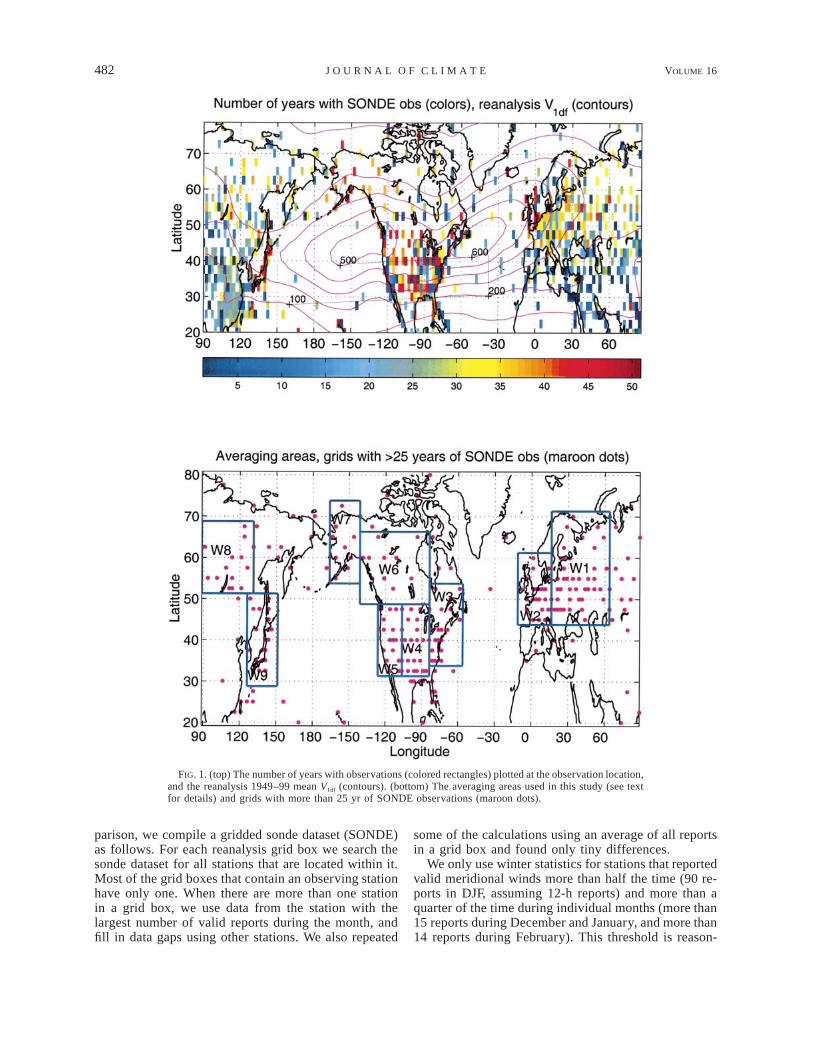
FIG. 3. The difference between V1df of the high and low decades of Fig. 2 for (top) SONDE and (bottom)RSAMP. Data are shown only for grids with at least 7 yr of observations in each of the decades.

TABLE 1. Geographic characteristics of the averaging areas used in this study (shown in Fig. 1).

Region Storm track part Longitude range Latitude range

W1W2W3W4W5W6W7W8W9

Eastern EuropeWestern EuropeEastern United StatesCentral United StatesWestern United StatesCanadaAlaskaSiberiaJapan

Atlantic exit—downstreamAtlantic exitAtlantic entrancePacific exit—downstreamPacific exitPacific exit, North branchPacific North edge

—Pacific entrance

16.258–63.758E11.258W–16.258E83.758–56.258W

106.258–83.758W1268–106.258W

141.258–83.758W166.258–141.258W

88.758–131.258E126.258–151.258E

43.758–71.258N43.758–61.258N33.758–53.758N31.258–48.758N31.258–48.758N48.758–68.758N53.758–73.758N51.258–68.758N28.758–51.258N

storm track, but no station at the peak itself. From Fig.2, it is apparent that the SONDE variance agrees wellwith reanalysis data during the 1990s, but the agreementis not as good during the earlier decade, when the re-analysis appears to be biased low.

Figure 3 shows the difference between the 1990–99and 1962–71 decadal means (denoted by D10V1df), forSONDE and the sampled reanalysis, RSAMP, for gridboxes that have V1df observations for 7 or more yearsof each decade. We see that the reanalyses shows stron-ger storm tracks in the 1990s compared to the 1960s,while SONDE shows an intensification in Northern Eu-rope, western United States, western Canada, and the

northern part of Japan, but the intensification is weakerthan in the reanalysis. Over the central and eastern Unit-ed States, southern Europe along the Mediterraneancoast, and the southern part of Japan, SONDE showsno significant difference in storm track strength betweenthe two decades, while RSAMP shows some intensifi-cation. Since the two datasets, SONDE and RSAMP,have the same spatial and temporal sampling, our resultssuggest that there are biases in the reanalysis.

The differences between sonde and reanalysis dataappear to have a spatial pattern. To get a more detailedpicture, we look at area averages of V1df. This also allowsus to study the time evolution of the storm tracks, and


FIG. 4. The yearly time series of the total number of stations with sufficient observations, in multiplesof 10 (dashed), and the area coverage index for the areas shown in Fig. 1 (solid dots). See text for definitionof the index.

FIG. 5. Yearly time series of the area averages of 300-hPa V1df forareas W1, W2, W3, W5, W6, and W9 of Fig. 1. Shown are SONDE(thick dotted line) and RSAMP (thin line).

determine how representative the decadal mean differ-ences are of the full time evolution.

The averaging areas we use are shown in the bottomplot of Fig. 1, and their geographical characteristics arelisted in Table 1. The areas were defined to represent dif-

ferent regions of the storm tracks, taking into account thedistribution of observations. For reference, we also markall grid points that have more than 25 yr of SONDE ob-servations on the figure showing the averaging areas. Wealso tried other area divisions, and the overall results arethe same. Figure 4 shows the mean number of sonde sta-tions that had a sufficient amount of observations in eacharea (dashed line, in multiples of 10). We see that thenumber of stations changed quite a lot over the years, witha strong increase in early years and a roughly constantnumber afterwards, with a decrease in the 1990s for someareas. We also define an area-coverage index by dividingeach area into nine (3 3 3) roughly equal subareas andcounting how many subareas have at least one station witha sufficient number of reports, for each year. Figure 4shows the coverage index for each of the averaging areas(dots). We see that the index changes drastically duringthe early 1950s in most areas, before 1965 in W6, and fora few single years in W1 and W8. Since large changes ofthis index indicate possible trends due to changes in areacoverage, we only look at area averages from 1958 on-ward, and regard area 6 data with caution before 1965.Note that a substantial increase in the number of rawind-sonde stations in early years occurred after the Interna-tional Geophysical Year in 1957 (Kistler et al. 2001).

Area averages are calculated as a simple average of all


TABLE 2. The linear trend (m2 s22 yr21) of the area mean time seriesof V1df from 1958–99 for SONDE and RSAMP data. Trends with asignificance level .0.95 and ,0.80 are bold and italic, respectively.

Area SONDE RSAMP

W1W2W3W5W6W9

3.041.731.311.273.030.66

4.103.572.172.523.822.58

FIG. 7. SONDE minus RSAMP yearly time series (the differencebetween the curves in Fig. 5, thick dotted line) and REAN minusRSAMP (thin line).

FIG. 6. The 10-yr running means of the time series in Fig. 5 (usingthe same line types).

FIG. 8. The average of all area mean V1df time series except forW8, for SONDE and RSAMP as well as for the corresponding fullreanalysis curve (REAN). SONDE (thick dotted line), RSAMP (thinline), and REAN (dashed).

observations in a given area. Figure 5 shows the yearlytime series of the area averages of SONDE and RSAMP,for six of the areas representing the main storm trackentrance and exit regions, while their difference is shownlater in Fig. 7, as the thick dotted line. We do not showresults from areas W4, W7, and W8. Unless otherwisenoted, the results from area W4 are similar to W5. AreaW7 shows no trend in storm track strength, even in thereanalysis, and area W8 is outside the main storm trackregion. The linear trends for the period 1958–99, alongwith the significance levels are shown in Table 2.1

We see large decadal timescale variations in the stormtrack strength in SONDE, as well as reanalysis data.The variance in the reanalysis is generally less than thatin radiosonde data, and the difference is too large to beaccounted for by the presumed observational error ofrawindsonde wind observations. Overall, the biases inthe reanalysis (best shown in Fig. 7) are larger in the60s and early 70s than in the 80s and 90s. As a result,the positive trend in storm track strength is weaker inSONDE data than in the reanalysis. Figure 6 shows the10-yr running means of these time series. Comparingthe decadal means around 1965 and 1995 (Fig. 6), we

1 The significance levels are computed using a two-tailed t testassuming all data are independent.

see that the decadal mean in the 90s is significantlystronger than that in the 60s for all areas shown, inagreement with CF, but the differences in SONDE datain areas W2, W5, and W9 are substantially smaller thanthose in RSAMP. Examining the full time evolution inmore detail, we find that over the Atlantic entrance andEurope (regions W3, W1, W2) the storm tracks showa positive trend in reanalysis and SONDE data, but theSONDE trend is weaker and less significant thanRSAMP in areas W2 and W3 and slightly weaker inarea W1. In the Pacific areas (W5, W6, W9) the re-analysis shows a decadal timescale oscillation with anoverall positive trend while SONDE shows the oscil-lation but almost no trend in area W9, a somewhat weak-er and less significant trend in W5, and a large positivetrend in area W6.

It is also illuminating to look at the temporal evolution


FIG. 9. The relative change in V1df during the early 1970s [(1974 2 1971)/1971], for (top) SONDE,and (bottom) RSAMP.

of the mean of V1df over all averaging areas, which issome measure of the strength of the hemispheric stormtrack, at least over land areas. Figure 8 shows the yearlytime series using a simple mean (weighting by the geo-graphic area of the averaging regions makes no differ-ence), for SONDE and RSAMP.2 To examine the effectsof spatial sampling on the area averages, we also cal-culate them from the full reanalysis dataset, weightedby cosine latitude (referred to as REAN), and plot it inFig. 8 using a dashed line. The first thing to note is thesimilarity in the year-to-year variation of the differentdatasets, which is also remarkably similar to the yearlyvariability of the first PC of the reanalysis [the corre-lation between REAN and the dashed line of Fig. 11(to be shown later) is 0.93]. On longer timescales,SONDE and the reanalysis datasets differ more. Thereanalysis shows a transition in the early 1970s from aweaker to a stronger storm track regime. The SONDEstorm track, on the other hand, only shows a hint ofthis transition. There is a strong intensification in the

2 The averages shown in Fig. 8 are for an average using all areasexcept W8. This is done because W8 has a few years of missing datain the 1990s. We get similar results, however, when we do includeit in the average.

early 1970s, leading to a peak in 1975. SONDE valuesare stronger than the reanalysis, as expected, but theSONDE–reanalysis biases are largest in the 1960s andearly 1970s, resulting in an overall trend that is muchweaker in sonde data (1.34 m2 s22 yr21 in SONDE com-pared to 2.52 m2 s22 yr21 in RSAMP, both with .0.999significance level).

Another feature we examine using sonde data is thetransition, during the early 1970s, from a weak to strongstorm track regime, found in the reanalysis PC timeseries by CF. Since such a transition can result fromchanges in the reanalysis, it is important to verify it insonde data. Chang and Fu (2002) found evidence of anintensification in the early 1970s in a small subset ofthe sonde stations, suggesting it is a real feature. Thehemispheric storm track time series (Fig. 8) also showsan intensification during 1969–75 in SONDE data, butunlike the reanalysis time series, in SONDE data it looksmore like a temporary peak than a transition from weakto strong storm track regimes. We also look at thechange in the storm tracks for 1971–74 (Fig. 9). Boththe sonde and reanalysis data show the storm tracksintensified significantly in 1971–74 over Europe, theeastern Atlantic, the United States, and central Siberia,and weakened around the western and northern edges


FIG. 10. The first EOF of (top) SONDE and (bottom) RSAMP data, only using grid points with morethan 25 yr of observations (colored rectangles). Also shown in the bottom plot is the first EOF of the fullreanalysis data (contours). The EOFs are normalized to represent one std dev. To facilitate comparison, thesame color scheme is used for SONDE and RSAMP and the reanalysis.

of the Pacific storm track. Over the Atlantic storm trackexit (eastern Atlantic and Europe) the intensification isweaker in SONDE data.

Its hard to conclude from the existing SONDE datawhether the Pacific storm track changed much during1971–74, since there is very little data from the Pacificstorm track maximum region. Over the locations of theweather ships in the eastern Pacific (508N–1458W,308N–1408W), the reanalysis data show a weak inten-sification, but the SONDE data show no significant in-tensification. In the SONDE data, the intensification isweaker along the western U.S. coast, but is quite strongover the rest of the United States.

b. An EOF analysis of the variability of the stormtracks

In this section, EOF analysis is used to determinewhether the significant correlation between the Atlanticand Pacific storm tracks, and the transition in the early1970s from a weak to a strong storm track regime, bothfound in reanalysis data (CF), also exists in sonde data.We calculate the EOFs from the eigenvalues of the co-variance matrix of the data, and the PC time series are

then calculated from the projection of the data onto theEOFs. Each element of the covariance matrix is cal-culated only from years for which data exists for bothof the corresponding grid points. This method does notrequire any time interpolation of the data. For the resultsto be meaningful, we only use grid points that have atleast 25 yr of observations. For the EOF calculations,we weigh each grid point by the square root of cosinelatitude, to account for the difference in grid area, andby the square root of the number of years of existingobservations (the variances are weighted by the cosineof latitude and the number of observations). Figures 10and 11a show the resulting EOF and PC time series, forSONDE and RSAMP. For comparison, we also plot theEOF and PC time series calculated by CF from the fullreanalysis dataset. Table 3 shows the percent of varianceaccounted for by the first EOFs, and their linear trends.

Comparing RSAMP and the full reanalysis, we seethat our analysis does produce meaningful results. Theoverall EOF pattern that emerges from the scattered gridpoints of RSAMP is similar to the full reanalysis, withthe main differences being somewhat smaller loadingsfor RSAMP over eastern Europe, China, and Japan.Over the location of the two weather ships near the peak


FIG. 11. The first PC time series corresponding to the EOFs shownin (top) Fig. 10, (middle) Fig. 12 (Atlantic), and (bottom) Fig. 12(Pacific): SONDE (thick dotted line), RSAMP (thin line), and the fullreanalysis (dashed). PCs are in units of std dev.

TABLE 3. The percent of variance explained by the first EOF cal-culated using SONDE, RSAMP, and the full reanalysis datasets, forNH, ATL, and PAC, as well as the linear trend of the correspondingPC time series (in parentheses, in units of std dev per year). Thesignificance levels of the trends are very high (all are .0.97, withmost exceeding 0.99) except for SONDE PAC, for which the sig-nificance level is 0.53.

Areasused SONDE RSAMP

Fullreanalysis

NHATLPAC

16 (0.022)25 (0.024)27 (0.007)

25 (0.034)36 (0.032)36 (0.022)

29 (0.051)35 (0.041)43 (0.043)

of the Atlantic storm track, the EOF loadings have asmaller value than the full reanalysis, probably becausethey only existed in earlier years, when the storm trackwas weaker. The year-to-year variability of the PC ofRSAMP is very similar to the full reanalysis, with theircorrelation being 0.80. The reanalysis time series issmoother, and correspondingly, RSAMP has more ex-treme values, most notably the much stronger peak in1974. In addition, the trend in the reanalysis PC is sig-nificantly stronger than the RSAMP one, suggesting thestorm track increased more over the ocean than overland.3 Nevertheless, the similarity between RSAMP andthe reanalysis also suggests that an EOF analysis basedonly on land data is indicative of the variability of thefull storm tracks. We also performed a series of sensi-tivity tests that show the robustness of our results. Wedescribe these in appendix B.

Comparing SONDE and RSAMP (in Figs. 10 and11a) we see that the EOF patterns are remarkably sim-

3 We verify that the differences are not due to temporal samplingby repeating our calculations using the reanalysis at all synoptic time-scales, which gives results very similar to the RSAMP PCs.

ilar, with the largest difference over eastern Europe,China, and Japan, where the SONDE EOF loading isclose to zero, while the reanalysis is small but mostlypositive. The SONDE EOF accounts for less of the totalvariance, compared to the reanalysis (Table 3), but thelargest differences are in the PC time series. Consistentwith our previous findings of an overall smaller positivetrend (see Table 2), SONDE values are larger than thereanalysis before the mid 1970s and smaller after that,with the trend clearly apparent only when looking at the10-yr running means [see Fig. 13 (shown later)]. Oneof the striking features in all the PCs is the strong in-tensification of the storm tracks during the early 1970s,but while in the reanalysis (especially using the fulldataset) this coincides with a transition from weak tostrong storm track regimes, in SONDE data most of theintensification is temporary, with a small overall inten-sification that is clearly noticeable only when lookingat longer timescales (e.g., as shown later in Fig. 13).

A more detailed picture is obtained from looking atthe individual oceanic storm track EOFs. Figure 12shows the first EOFs for the Atlantic (ATL) and Pacific(PAC) regions. These are calculated separately, usingall grid points between 1208E to 1008W and 908W to508E for PAC and ATL, respectively. Table 3 shows thepercent variance accounted for by the correspondingPCs, as well as the linear trends. Compared to the fullEOF (denoted by NH), the EOF loadings over Japan arestronger in PAC than in NH, for all datasets. The At-lantic entrance, on the other hand, is weaker in ATLcompared to NH. These differences are largest forSONDE and are quite small for RSAMP. The PC timeseries, including the full reanalysis, are shown in Fig.11b,c, and the corresponding linear trends are shown inTable 3 (in parentheses). We see again that SONDEvalues are generally larger than the reanalysis before1976, and smaller afterward, resulting in an overallweaker positive trend. We see an intensification of theAtlantic storm track after the early 1970s, resulting inan overall trend that is clear even in SONDE data. Inthe Pacific, however, there does not seem to be muchof a trend in SONDE data (a linear fit gives 0.007 stan-dard deviations per year, with a significance level of0.53, compared to 0.022 standard deviations per yearand a significance level of 0.99 for RSAMP). The


FIG. 12. The same as Fig. 10 but for the first EOFs calculated separately for the Atlantic and Pacificstorm track regions.

TABLE 4. The correlations between various PC time series for thefull dataset (NH), the Atlantic (AT), and the Pacific (PA) storm trackregions, and for SONDE (S), and RSAMP (RS) for each region. Pa-rentheses denote values that are not statistically significant, based ona 95% confidence level, but all other values are above the 99% percentconfidence level.

NH-S NH-RS AT-S AT-RS PA-S PA-RS

NH-SNH-RS

AT-SAT-RS

PA-SPA-RS

10.940.90—

0.65—

—1—

0.95—

0.65

——

10.96

(0.27)0.36

———

1(0.25)0.39

————

10.95

—————

1

SONDE time series looks more like a very strong peakin 1974 superposed on an overall very weak positivetrend. On the other hand, the trend in RSAMP is onlyabout half that in the full reanalysis, suggesting a largepart of it comes from ocean regions, which are not cov-ered by the SONDE network. An examination of aircraftdata, which exists over the oceans, should be useful forresolving this issue. This is currently being done.

This leads us to examine the relation between theAtlantic and Pacific storm tracks. Table 4 shows thecorrelation between various PC time series. We find that

while the Pacific and Atlantic storm tracks are signifi-cantly correlated in reanalysis data, with a correlationof 0.39 for RSAMP (0.36 is the 99% confidence level),they are only marginally significantly correlated inSONDE data (0.27, with 0.28 being the 95% signifi-cance level). This difference in correlation is a bit sur-prising, given that the year-to-year variability ofSONDE and RSAMP are quite similar (with SONDE–RSAMP correlations higher than 0.91 for NH, ATL, andPAC). The differences become clear when we look atlonger timescales. Figure 13 shows the 10-yr runningmeans of the NH, ATL, and PAC PC’s, for the two da-tasets. We see that on long timescales, ATL and PACdiffer much more in SONDE than in the reanalysis da-tasets, with an ATL–PAC correlation of the 10-yr runningmeans of 0.06 for SONDE, compared to 0.55 forRSAMP.4 This suggests that the reanalysis introduces aspurious correlation between the storm tracks on longtimescales. Indeed, when we detrend the PC time series

4 Note that while ATL RSAMP and PAC SONDE are marginallysignificantly correlated (0.25, see Table 4), PAC RSAMP and ATLSONDE are significantly correlated (0.36 and 0.40), suggesting thatthe correlation in the reanalysis is introduced through the Pacificstorm track.


FIG. 13. The 10-yr running means of the PC time series of Fig.11, for (top) SONDE and (bottom) RSAMP. Curves are for NH (1),ATL (V), and PAC (*).

TABLE 5. Statistics of the SVD analysis of the cross covariance matrix of the Pacific and Atlantic storm track regions. The significancelevels of the trends exceed 0.989 for RSAMP and are 0.97/0.62 for SONDE ATL/PAC.

DatasetATL–PACcorrelation

Squaredcovariance (%)

Variance (%)ATL/PAC

Linear trend (s/yr21)ATL/PAC

Correlation with first PCATL/PAC

SONDERSAMP

0.610.58

44.666.5

17.2/23.029.2/32.4

0.029/0.0100.051/0.028

0.95/0.730.98/0.70

before correlating them, the ATL–PAC correlations dropto 0.28 and 0.25 for RSAMP and SONDE, respectively.

One possible source of a spurious correlation on longtimescales is the low bias in the early years in the re-analysis, which introduces a ‘‘spurious jump’’ in thetime series. We test this by removing a step functionfrom the ATL and PAC RSAMP PC time series, to makethe difference between the means of 1949–72 and 1976–99 be the same as in the corresponding SONDE PC timeseries. The resulting correlations are in the ranges of0.26–0.28 for RSAMP, with the actual values dependingon how we vary the time series between 1972 and 1976,suggesting the time evolution of the reanalysis biasesintroduces much of the spurious correlation in RSAMP.5

We note, however, that EOF analysis does not max-imize correlations. A better approach is to perform asingular value decomposition (SVD) analysis of thecross covariance matrix of the two storm track regions,

5 These results appear to suggest that the two storm tracks are notsignificantly correlated—even in the reanalysis data—after the ‘‘spu-rious jump’’ in the reanalysis bias is removed. However, note thatCF computed the correlation between the leading ATL and PACmonthly mean PCs based only on DJF months after 1976 and foundsignificant correlation between the two storm tracks in both NCEP–NCAR and ECMWF reanalysis data—due to significant correlationbetween the two storm tracks over the oceanic regions, over whichwe do not have sufficient data to verify.

since this maximizes the covariance between the two(Bretherton et al. 1992, see appendix of CF). The re-sulting SVD patterns (not shown) look similar to thecorresponding EOF of each storm track region, with theexit regions being stronger than the entrance regions,especially in the Pacific. The SVD time series are highlycorrelated with the corresponding NH first PC time se-ries. These correlations, along with the main results ofthis analysis, are summarized in Table 5. We see a sig-nificant correlation between the storm tracks for all da-tasets of around 0.6, with SONDE being slightly largerthan RSAMP. The leading SVD mode, however, ex-plains a smaller percentage of the squared covariancein SONDE data (44.6% for SONDE vs 66.5% forRSAMP, respectively). Correspondingly the individualSVD patterns in SONDE data explain a smaller percentof the variance in each individual basin (17.2%/23.0%ATL/PAC for SONDE, compared with 29.2%/32.4% forRSAMP). This supports our earlier conclusion, that thereanalysis data introduce some spurious correlation be-tween the storm tracks. Finally, in accordance with ourprevious findings, the SVD analysis shows a positivelong-term linear trend for both storm tracks but strongerin the Atlantic, and a significantly weaker trend inSONDE data compared with the reanalysis.

c. The effects of spatial and temporal sampling

The comparison of SONDE and RSAMP data givesus an idea of the biases in the reanalysis, but it doesnot account for all of the differences between obser-vations, based on the full reanalysis and raw SONDEdata, that may also arise due to the effects of spatialand temporal sampling. We discuss these in the follow-ing section. We examine the effects of temporal sam-pling by repeating our calculations using the reanalysisdata at SONDE stations, and all synoptic timescales,and comparing to RSAMP. We also examine the effectsof spatial sampling on the area averages, by comparingRSAMP to area averages using the full reanalysis data,weighted by cosine latitude. Their difference, which isplotted as the thin line in Fig. 7, includes the effects oftemporal and spatial sampling. We see from Fig. 7 thatthe effects of spatial and temporal sampling are on thewhole smaller than the biases between SONDE andRSAMP, with a few exceptions.

Temporal and spatial sampling result in an overesti-mation of the linear trends in area W1 (suggesting thetrend may be even smaller than indicated by SONDE),and an underestimation of the trend in area W3. In area


W4 (central United States, not shown) the reanalysisshows an overall positive trend, while SONDE does not.Some of this difference is due to spatial and temporalsampling. Temporal sampling, in particular, results in alarge underestimation of the storm tracks in the 1980sand 1990s, suggesting actual SONDE values may belarger than shown during these years, and the lineartrend might be larger. One source of bias may be thefact that the reanalysis data is calculated using four dailyreports, while sonde observations were usually takenonly twice a day. A comparison of reanalysis variancesbased on 0000 and 1200 GMT, vs 0600 and 1800 GMTsuggests this does indeed introduce a bias of the ob-served sign, but it can only account for about a thirdof the difference. The distribution of the observationsbetween the three winter months is quite constant overthe United States during most of the observation period,suggesting the source of this bias is not straightforward,and requires further investigation. In area W6, before1965, both the spatial and temporal sampling were poor(see Fig. 4), resulting in a large underestimation of thestorm tracks during the early years, which suggests theSONDE trend might be an overestimate.

We also find that temporal sampling results in anunderestimation of the intensification in the early 70s(the difference 1974–71).

The effects of temporal sampling on the EOF andSVD analyses is mostly to decrease the percentage ofvariance that the various EOFs and SVD patterns ex-plain, by about 3%–4% variance (e.g., from 29% forthe first NH EOF using the dataset with all synoptictimes, to 25% for RSAMP). In addition, sampling de-creases the correlation between the Atlantic and PacificPC time series. For example, we get correlations of 0.39and 0.46 (0.36 is the 99% confidence level) for theyearly PC time series using RSAMP and the corre-sponding reanalysis dataset using all synoptic times, andcorrelations of 0.55 and 0.76 for the 10-yr running meantime series (as in Fig. 13).

4. Discussion and conclusions

To summarize, we find that the intensification of theAtlantic storm track found in the reanalysis data is alsofound in sonde data from the Atlantic exit and entranceregions, but weaker. The weaker trend is due to the factthat the biases between the reanalysis and sonde datahave, on the whole, decreased with time. In the Pacificregions, the reanalysis shows an interdecadal oscillationsuperposed on a positive trend. There is strong evidenceof the decadal timescale oscillations, but not of the pos-itive trend, in sonde data from the Pacific storm trackentrance and exit regions. It is possible that an inten-sification of the Pacific storm track did occur, but thesonde data is too sparse to say anything about it. Anortheastward shift along with the intensification could,in that case, explain the fact that a positive trend is notobserved over Japan and the central United States (W4),

is observed to be weak over the west coast of the UnitedStates (W5), and is quite strong over Canada (W6).

In this paper, we find a major change in the differencein variances between the sonde data and reanalysis dataoccurring during the early 1970s. During that time, therewas no major change in the observational network itself(apart from an increasing number of satellite observa-tions, which does not have a significant impact on theanalysis over the Northern Hemisphere. See, e.g., Moet al. 1995), but in 1973, a new scheme of encodingrawindsonde data (the ‘‘NMC Office Note 29’’ scheme,see Kistler et al. 2001) was introduced, enabling betterquality control as well as more efficient error detectionand correction (of temperature and height data) basedon hydrostatic consistency. Note that this change doesnot directly affect the SONDE dataset, but it affects thereanalysis in the way the SONDE data are assimilated.Thus any changes in the biases between the two datasetsover this time period basically reflects changes in thequality of the reanalysis data. The fact that the forecastsusing the reanalysis dataset as initial conditions show ajump in skill around that time (Kistler et al. 2001, theirFig. 7) suggests that the quality of the reanalysis isimproved after that time, which is consistent with ourresult that the difference between radiosonde and re-analysis variances is much smaller after the early 1970s(Fig. 7). Thus, our results indicate that the storm trackintensity in the reanalysis dataset is biased low beforethe early 1970s, and part of the jump in storm trackintensity seen in the PC time series based on the re-analysis data at that time is probably due to this bias.

Nevertheless, the sonde data still display a markedincrease in storm track intensity during the early 1970s,especially over the Atlantic sector. This increase is sug-gestive of a transition between weak and strong stormtrack regimes (especially in the reanalysis data and lessso in the sonde observations), which could be an in-dication of a larger-scale climate regime change. In fact,the North Atlantic Oscillation (NAO) index (the nor-malized pressure difference between Portugal and Ice-land) has been anomalously high since the early 1970s,compared to the 1864–1994 time series (Hurrell 1995).Seager et al. (2000) performed an SVD analysis on SSTand surface winds for the Atlantic basin, and the SSTtime series showed a transition from low to high valuesin the early 1970s (their Fig. 6c). Chang and Fu (2002)also found that the Atlantic storm track intensity is wellcorrelated with the NAO index (see also Geng and Sugi2001) as well as the Arctic Oscillation index (Thompsonet al. 2000). There is also much evidence of a climateregime change in 1977, seen most strongly over thePacific basin, in various indices based on pressure, SST,and ocean subsurface temperature (e.g., Trenberth 1990;Mantua et al. 1997; Deser et al. 1999, and referencestherein), but the few year time lead of the storm tracksneeds to be explained if these transitions are to be re-lated. Graham and Diaz (2001) suggested that the Pacificstorm track intensification could be related to a decadal


trend observed in ENSO (e.g., Zhang et al. 1997); butCF found that the Pacific storm track intensity is onlyweakly correlated with the Southern Oscillation index(SOI), with much of the decadal variability and trendremaining even when storm track variations that arelinearly congruent with the high and low frequencycomponents of the SOI have been taken out. Anotherpossibility is that the intensification in the early 1970sled to a temporary peak in storm track strength, whichis not associated with any regime transition, and anobserved intensification over the past 30 yr could be anunrelated trend. Based on the SONDE data, the latterpossibility appears to be the more likely.

With regard to the correlation between the Pacific andAtlantic storm track anomalies, our analysis of the sondedata does show some correlation between the two stormtracks, especially over the storm track exits (where theSVD patterns of the two storm tracks are largest) butthe correlation appears to be somewhat weaker than thatshown in the reanalysis data. No definitive conclusioncan be drawn for this case, since much of the covariancebetween the two storm tracks found by CF occurs overthe oceans, where we do not have enough data to ad-dress.

Our results once again demonstrate how the analysisof long-term climate variability can be hampered by thelack of consistent, uninterrupted data records, especiallyover the oceanic regions. The decommissioning of theweather ships over the past few decades made it im-possible to verify the trend in storm track intensity overthe oceanic storm track peaks based on radiosonde dataalone. The large change in biases between the radio-sonde and reanalysis variance around the early 1970s,which has a magnitude dependent on geographical lo-cation, casts serious doubts on the magnitude of climatetrends determined on reanalysis data alone. In view ofthese uncertainties, more efforts have to be made tobetter determine the variability of the storm tracks overthe oceanic regions. Graham and Diaz (2001) made useof some in situ observations, as well as wave heightmeasurements and hind casts, to infer changes in stormtrack intensity. While those measurements do suggestan overall increasing trend in Pacific storm track activ-ity, it is difficult to quantify the actual amount that stormtrack activity has changed based on those observationssince they do not directly measure either cyclone activ-ity or eddy variance statistics near the storm track peak.We are in the process of analyzing aircraft observationsover the Pacific and Atlantic storm track regions to seewhether the trend in variances can be observed in air-craft observations.

Acknowledgments. Much of the work this paper isbased on was conducted when the authors were at TheFlorida State University, where they were supported byNSF Grant ATM-0003136, and NOAA GrantNA06GP0023. EC was also supported by a CRC awardat FSU, and NSF Grant ATM-0296076 at SUNYSB.

NH would also like to acknowledge the hospitality pro-vided by Professor R. Lindzen at MIT.

APPENDIX A

Possible Biases in Objectively Analyzed Variances

The spectral statistical interpolation (see Parish andDerber 1992) method used in the NCEP–NCAR re-analysis procedure is based on the principle of leastsquares estimation (see, e.g., Daley 1993). In this ap-pendix, we will consider least squares estimation of asingle variable at a single point based on combining asingle observation with a background first guess, in thiscase assumed to be a forecast from a model with knownbiases in the mean value that have been removed. Partsof the following discussions may seem trivial, but theyare presented here for the sake of completeness. Let tbe the unknown truth, a denote the analysis, b the back-ground guess, and o the observation value to be assim-ilated with b to produce the analysis, such that

a 5 b 1 w(o 2 b), (A1)

where w is the weight to be determined. In least squaresestimation, w is chosen a priori such that the expectedrms error in a,

2 1/2rmse 5 ^(a 2 t) & , (A2)

is minimized. Here ^ & represents the expectation op-erator. Under the assumptions that observational andforecast errors are uncorrelated, and that observationaland forecast mean biases have been removed, simplemanipulations (see, e.g., Daley 1993) give the well-known result

2^(b 2 t) &w 5 . (A3)

2 2^(b 2 t) & 1 ^(o 2 t) &

Assuming that we know the magnitude of the ex-pected observational and forecast error variances, theanalysis for a using Eq. (A1), making use of the weightw from Eq. (A3), is optimized in the sense that theexpected analysis error variance, ^(a 2 t)2&, is mini-mized by this procedure, and is guaranteed to be lessthan or equal to both the observational and forecast errorvariances.

However, this procedure does not guarantee that theanalyzed variance is necessarily a better estimate of thetrue variance than is the observed variance. Assumingthat biases (in the mean) have been removed, we cansubtract the mean value of each quantity from both sidesof Eq. (A1), squaring the equation, and taking the ex-pectation values on both sides; thus we get

2 2 2 2 2â9 & 5 (1 2 w) ^b9 & 1 w ô9 &

1 2w(1 2 w)ô9b9&. (A4)

Here, primed quantities denote deviation from the meanvalue. Let us assume that the observational errors arerandom; that is,


o9 1 t9 1 r, (A5)

where r is uncorrelated with t9 or b9. Further assumethat the first guess error is partly correlated with thetruth, and partly random—in other words, the forecasthas an amplitude error on top of random errors, that is,

b9 5 at9 1 s, (A6)

where s is uncorrelated with t9 (or o9). If a equals 1,the forecast errors and the truth are uncorrelated, butwhen a differs from 1, forecast errors are correlatedwith the truth. While one can argue that such a bias canbe easily corrected for in this example, in reality, if sucha bias occurs only over some limited regions in a globalmodel forecast, or only for some modes of variabilityout of many modes, this kind of bias is not correctedfor (or even easily recognizable) in the current objectiveanalysis procedures.

Using Eqs. (A5) and (A6), we get2 2 2 2 2 2 2ô9 & 5 ^t9 & 1 ^r &, ^b9 & 5 a ^t9 & 1 ^s &

2ô9b9& 5 a^t9 &. (A7)

Substituting Eq. (A7) into (A4) we get, for this example,2 2 2 2 2â9 & 5 [w 1 a(1 2 w)] ^t9 & 1 w ^r &

2 21 (1 2 w) ^s &. (A8)

If a equals 1, Eq. (A8) becomes2 2 2 2 2 2â9 & 5 ^t9 & 1 w ^r & 1 (1 2 w) ^s & (A9)

and, in this case, using Eqs. (A3), (A5), and (A6), theweight w is simply given by

2^s &w 5 (A10)

2 2^s & 1 ^r &

and it is clear from Eqs. (A9) and (A10) that the ex-pected error in the analyzed variance, â92& 2 ^t92&, issmaller than either ^r2& or ^s2&.

However, if a is not 1, the expected error in the an-alyzed variance is no longer guaranteed to be smallerthan ^r2&, the expected error in the observed variance.As a counter example, assume that a equals 1.1, suchthat b9 5 1.1t9 1 s. Hence ^(b9 2 t9)2& 5 0.01 ^t92& 1^s2&. Also, assume that ^s2& 5 0.01 ^t92&, hence the totalforecast error variance, ^(b9 2 t9)2& 5 0.02 ^t92&. Further,assume that the observational error variance equals 8%of the true variance, that is, ^(o9 2 t9)2& 5 ^r2& 5 0.08^t92&. From Eq. (A3), for this example, w 5 0.2, and wecan calculate that the expected analysis error variance,^(a9 2 t9)2& 5 0.016 ^t92&, indeed smaller than both theobservational or forecast error variances, as expected.However, from Eq. (A8), we find that for this example,â92& 5 1.176 ^t92&, whereas ô92& 5 1.08 ^t92&, hence theerror in the analyzed variance is larger than the error inthe observed variance. This is due to the fact that while^(b9 2 t9)2& 5 0.02 ^t92&, ^b92& 5 1.22 ^t92&, because ofnonzero correlation between the forecast error and thetruth value.

The simple example above shows that the varianceestimated from least squares estimation is certainly notguaranteed to be better than the variance estimated basedon observations alone, even though the observations areused in the production of the analyses. This is true evenin the absence of any changes in the analysis system.In the presence of changes in the analysis system (e.g.,changes in observational network), the errors and biasesin variances (and covariances) introduced by the anal-ysis system will change with time, thus possibly dis-torting the temporal evolution of, or even completelymasking, climate change signals if changes in variancesor covariances are sought.

APPENDIX B

Sensitivity Tests of the EOF CalculationsWe repeated the EOF calculations described in sec-

tion 3b with different thresholds for the minimum num-ber of years of observations, ranging from 1 (using allthe available data) to 45 yr (out of 51 yr total). Theresulting PC time series are almost identical to eachother for thresholds up to 35 yr. Higher thresholds resultin too many stations being dropped out of the analysis.The corresponding EOFs are also very similar, with theadditional grid points for lower thresholds having smallvalues. The largest difference is for SONDE data overJapan, where the EOF loading is small, with a mix ofnegative (blue) and positive (green) values. As thethreshold is increased, the EOF loading over Japan shiftsfrom zero (a roughly even mix of negative and positivepoints) to a small but positive value. We also calculatedthe EOFs and PC time series without weighting by thenumber of years of observations, and with weightingeach covariance matrix element by the number of ob-servation pairs that contribute to its calculation, and gotvery similar results. Finally, we repeated the EOF anal-ysis with a coarse grid version of the dataset. The coarsegrids used were 58 3 58, 58 3 158, and 108 3 308(latitude by longitude) with the corresponding V1df gridvalues calculated as a simple average over all the ex-isting 2.58 3 2.58 V1df values in each coarse grid box.The resulting PCs are surprisingly insensitive to coarsegraining of the data. The corresponding EOFs have sim-ilar overall features, with positive values along the stormtrack latitude band, with peak values in the oceanicstorm track exit regions. The largest sensitivity is overJapan in SONDE data, where the EOF loadings aresmall, and the relative distribution of negative and pos-itive values changes slightly with the choice of coarsegrid. We conclude that our EOF estimates are suffi-ciently meaningful and robust to use for comparingsonde and reanalysis data.

REFERENCES

Blackmon, M. L., 1976: A climatological spectral study of the 500mb geopotential height of the Northern Hemisphere. J. Atmos.Sci., 33, 1607–1623.


Bretherton, C. S., C. Smith, and J. M. Wallace, 1992: An intercom-parison of methods for finding coupled patterns in climate data.J. Climate, 5, 541–560.

Chang, E. K. M., 2000: Wave packets and life cycles of troughs inthe upper troposphere: Examples from the Southern Hemispheresummer season of 1984/85. Mon. Wea. Rev., 128, 25–50.

——, and Y. Fu, 2002: Interdecadal variations in Northern Hemi-sphere winter storm track intensity. J. Climate, 15, 642–658.

——, S. Lee, and K. L. Swanson, 2002: Storm track dynamics. J.Climate, 15, 2163–2183.

Daley, R., 1993: Atmospheric Data Analysis. Cambridge UniversityPress, 457 pp.

Deser, C., M. A. Alexander, and M. S. Timlin, 1999: Evidence for awind-driven intensification of the Kuroshio Current extensionfrom the 1970s to the 1980s. J. Climate, 12, 1697–1706.

Ebisuzaki, W., and R. Kistler, 1999: An examination of data-con-strained assimilation. Proc. Second WCRP Int. Conf. on Re-analyses, Wokefield Park, United Kingdom, WCRP, WMO Tech.Doc. 985, 14–17.

Geng, Q., and M. Sugi, 2001: Variability of the North Atlantic cycloneactivity in winter analyzed from NCEP–NCAR reanalysis data.J. Climate, 14, 3863–3873.

Graham, N. E., and H. F. Diaz, 2001: Evidence for intensification ofNorth Pacific winter cyclones since 1948. Bull. Amer. Meteor.Soc., 82, 1869–1893.

Gulev, S. K., O. Zolina, and S. Grigoriev, 2001: Extratropical cyclonevariability in the Northern Hemisphere winter from the NCEP/NCAR reanalysis data. Climate Dyn., 17, 795–809.

Hurrell, J. W., 1995: Decadal trends in the North Atlantic oscillation:Regional temperatures and precipitation. Science, 269, 676–679.

Kalnay, E., and Coauthors, 1996: The NCEP/NCAR 40-Year Re-analysis Project. Bull. Amer. Meteor. Soc., 77, 437–471.

Kidson, J. W., and K. E. Trenberth, 1988: Effects of missing data onestimates of monthly mean general calculation statistics. J. Cli-mate, 1, 1261–1275.

Kistler, R., and Coauthors, 2001: The NCEP–NCAR 50-year reanal-

ysis: Monthly means CD-ROM and documentation. Bull. Amer.Meteor. Soc., 82, 247–267.

Lau, N.-C., 1978: On the three-dimensional structure of the observedtransient eddy statistics of the Northern Hemisphere wintertimecirculation. J. Atmos. Sci., 35, 1900–1923.

Mantua, N. J., S. R. Hare, Y. Zhang, J. M. Wallace, and R. C. Francis,1997: A Pacific interdecadal climate oscillation with impacts onsalmon production. Bull. Amer. Meteor. Soc., 78, 1069–1079.

Mo, K. C., X. L. Wang, R. Kistler, M. Kanamitsu, and E. Kalnay,1995: Impact of satellite data on the CDAS-reanalysis system.Mon. Wea. Rev., 123, 124–139.

Paciorek, C. J., J. S. Risbey, V. Ventura, and R. D. Rosen, 2002:Multiple indices of Northern Hemisphere cyclone activity, win-ters 1949–99. J. Climate, 15, 1573–1590.

Parrish, D. F., and J. C. Derber, 1992: The National MeteorologicalCenter’s statistical–interpolation analysis system. Mon. Wea.Rev., 120, 1747–1763.

Petterssen, S., 1956: Motion and Motion Systems. Vol. 1, WeatherAnalysis and Forecasting, McGraw-Hill, 428 pp.

Seager, R., Y. Kushnir, M. Visbeck, N. Naik, J. Miller, G. Krahmann,and H. Cullen, 2000: Causes of Atlantic Ocean climate vari-ability between 1958 and 1998. J. Climate, 13, 2845–2862.

Thompson, D. W., J. M. Wallace, and G. C. Hegrel, 2000: Annularmodes in the extratropical circulation. Part II: Trends. J. Climate,13, 1000–1016.

Trenberth, K. E., 1990: Recent observed interdecadal climate changesin the Northern Hemisphere. Bull. Amer. Meteor. Soc., 71, 988–993.

Wallace, J. M., G. H. Lim, and M. L. Blackmon, 1988: Relationshipbetween cyclone tracks, anticyclone tracks, and baroclinic waveguides. J. Atmos. Sci., 45, 439–462.

Whitaker, L. M., and L. H. Horn, 1984: Northern Hemisphere extra-tropical cyclone activity for the midseason months. J. Climatol.,4, 297–310.

Zhang, Y. M., J. M. Wallace, and D. S. Battisti, 1997: ENSO-likeinterdecadal variability: 1900–93. J. Climate, 10, 1004–1020.

Storm Track Variations As Seen in Radiosonde Observations ...

Documents

Transcript of Storm Track Variations As Seen in Radiosonde Observations ...