STORM SURGE ANALYSIS USING NUMERICAL AND STATISTICAL

TECHNIQUES AND COMPARISON WITH NWS MODEL SLOSH

A Thesis

by

MANISH AGGARWAL

Submitted to the Office of Graduate Studies of Texas A&M University

in partial fulfillment of the requirements for the degree of

MASTER OF SCIENCE

August 2004

Major Subject: Ocean Engineering

STORM SURGE ANALYSIS USING NUMERICAL AND STATISTICAL

TECHNIQUES AND COMPARISON WITH NWS MODEL SLOSH

A Thesis

by

MANISH AGGARWAL

Submitted to Texas A&M University in partial fulfillment of the requirements

for the degree of

MASTER OF SCIENCE

Approved as to style and content by:

Billy L. Edge Cheung. H. Kim

(Chair of Committee) (Member) Douglas Sherman Paul N. Roschke

(Member) (Head of Department)

August 2004

Major Subject: Ocean Engineering

iii

ABSTRACT

Storm Surge Analysis Using Numerical and Statistical Techniques and Comparison with

NWS Model SLOSH. (August 2004)

Manish Aggarwal, B.E., Delhi College of Engineering,

Delhi, India

Chair of Advisory Committee: Dr. Billy Edge

This thesis presents a technique for storm surge forecasting. Storm surge is the

water that is pushed toward the shore by the force of the winds swirling around the storm.

This advancing surge combines with the normal tides to create the hurricane storm tide,

which can increase the mean water level by almost 20 feet. Numerical modeling is an

important tool used for storm surge forecast. Numerical model ADCIRC (Advanced

Circulation model; Luettich et al, 1992) is used in this thesis for simulating hurricanes. A

statistical technique, EST (Empirical Statistical Technique) is used to generate life cycle

storm surge values from the simulated hurricanes. These two models have been applied to

Freeport, TX. The thesis also compares the results with the model SLOSH (Sea, Lake,

and Overland Surges from Hurricanes), which is currently used for evacuation and

planning. The present approach of classifying hurricanes according to their maximum

sustained winds is analyzed. This approach is not found to applicable in all the cases and

more research needs to be done. An alternate approach is suggested for hurricane storm

surge estimation.

iv

DEDICATION

To God and my family for guiding me throughout my life

v

ACKNOWLEDGMENTS

This research was conducted at Texas A&M University and was supported by the

Department of Civil Engineering, Texas A&M University through the Texas Engineering

Experiment Station (TEEX).

I would like to thank my Chair Dr. Billy Edge for his guidance and contribution in

my understanding of this research and coastal engineering as a whole. I would also like to

thank my advisory committee members: Dr. C. H. Kim and Dr. Douglas Sherman for

their trust and guidance throughout this research project.

I also wish to thank my fellow classmates and friends for their active help and

contribution: Dr. Wahyu Pandoe, Mr. Young-Hyun Park, and Mr. Oscar Cruz Castro.

The thesis would not have been possible without the interest shown by Mr. George

Kidwell and Mr. Mel McKey of the Velasco Drainage District who made substantial

contributions to the completion of this modeling study.

Special thanks to my family for their constant support and motivation without

which, I would have never come this far.

vi

TABLE OF CONTENTS Page

ABSTRACT....................................................................................................................... iii

DEDICATION................................................................................................................... iv

ACKNOWLEDGMENTS……..……………………………………..………………… v

LIST OF FIGURES……………………..………………………………..…………… viii

LIST OF TABLES……………………….……………………………………………….x

1 INTRODUCTION ...................................................................................................... 1

1.1 Motivation........................................................................................................... 1 1.2 Approach............................................................................................................. 3 1.3 Study Area .......................................................................................................... 4 1.4 Procedure ............................................................................................................ 5 1.5 Outline .............................................................................................................. 10

2 ADCIRC: MODEL DESCRIPTION ........................................................................ 11

2.1 ADCIRC Model ................................................................................................ 11 2.2 Tidal Propagation.............................................................................................. 17 2.3 Bottom Stress.................................................................................................... 19 2.4 Wind Forcing .................................................................................................... 20

3 SLOSH...................................................................................................................... 29

3.1 Development of SLOSH................................................................................... 29 3.2 SLOSH Methodology ....................................................................................... 33 3.3 SLOSH Output.................................................................................................. 34

4 THE EMPIRICAL SIMULATION TECHNIQUE .................................................. 36

4.1 Storm Consistency with Past Events................................................................. 38 4.2 Storm Event Frequency .................................................................................... 40 4.3 Risk-Based Frequency Analysis ....................................................................... 41 4.4 Frequency-of-Occurrence Relationships .......................................................... 41

5 PROJECT IMPLEMENTATION............................................................................. 44

5.1 Coastline ........................................................................................................... 44 5.2 Bathymetry........................................................................................................ 45 5.3 Grid Generation ................................................................................................ 45 5.4 Boundary Conditions and Model Setup............................................................ 45 5.5 Tidal Verification.............................................................................................. 49

vii

Page

5.6 Tropical Storm Surge………………………………………………………….54 5.7 Application of EST……………………………………………………………66

6 COMPARISON WITH SLOSH ............................................................................... 73

6.1 Methodology of Storm Atlas ............................................................................ 73 6.2 Maximum Envelope of Waters (MEOW)......................................................... 74 6.3 Storm Atlas for Harris/ Brazoria County.......................................................... 75 6.4 Comparison with ADCIRC............................................................................... 77 6.5 Alternate Approach........................................................................................... 84 6.6 Validation.......................................................................................................... 87

7 CONCLUSIONS....................................................................................................... 94

REFERENCES ................................................................................................................. 97

APPENDIX A ………………………………………………………………………….100

APPENDIX B………………………………………..…………...…………………….116

APPENDIX C..………………………………………..………………………………..191

VITA………………………………………………….………………………………...202

viii

LIST OF FIGURES

Page

Fig. 1-1 Study area.............................................................................................................. 5

Fig. 1-2 Computational domain .......................................................................................... 8

Fig. 1-3 Bathymetry in the computational domain ............................................................. 9

Fig. 1-4 Grid resolution in the region of interest ................................................................ 9

Fig. 1-5 Bathymetry in the area of interest ....................................................................... 10

Fig. 2-1 Nomograph from Jelesnianski and Taylor (1973) used to derive radius of maximum winds from given maximum surface winds (long term average, no gusts) .......................................................................................................... 23

Fig. 2-2 Nested grid system used for hurricane wind computation .................................. 26

Fig. 2-3 Plot of variation of wind stress for a well-developed hurricane moving towards Texas coast ........................................................................................ 28

Fig. 3-1 SLOSH model basins for the East and Gulf coastlines of the U.S...................... 31

Fig. 3-2 SLOSH model basin for Galveston Bay ............................................................. 32

Fig. 5-1Comparison of tides at Freeport Harbor............................................................... 51

Fig. 5-2 Comparison of tides at Pleasure Pier.................................................................. 52

Fig. 5-3 Comparison of tides at Pleasure Pier with NOS gage......................................... 53

Fig. 5-4 Wind speeds at Pleasure Pier .............................................................................. 53

Fig. 5-5 Large and small scale plots of Hurricane Claudette’s track................................ 57

Fig. 5-6 Raw surface elevation data for Hurricane Claudette at Freeport Harbor............ 59

Fig. 5-7 Surge only surface elevation data for Hurricane Claudette................................. 60

Fig. 5-8 Simulated-observed data for Hurricane Carla (1961) for Pleasure Pier.............. 63

Fig. 5-9 Simulated-observed data for Hurricane Alicia (1983) for Pleasure Pier ............ 63

ix

Page

Fig. 5-10 Maximum surge at the approximate time of peak surge for Hurricane Claudette along the area of Freeport coast................................................... 64

Fig. 5-11 Location of points used for input to EST model ............................................... 67

Fig. 5-12 Frequency relationship for the Freeport Harbor for 500 simulations of 200 years. ............................................................................................................ 69

Fig. 5-13 Mean value of surface elevation with standard deviation bounds for Freeport Harbor............................................................................................ 70

Fig. 5-14 200 year storm surge values around the Freeport Levee system....................... 71

Fig. 5-15 100 year storm surge values around the Freeport Levee system....................... 71 Fig. 5-16 50 year storm surge values around the Freeport Levee system………………..72

Fig. 6-1 MEOW for Hurricane Carla (1961) for Galveston Bay (units of elevation are in feet (Jelesnianski 1992)) ............................................................................ 76

Fig. 6-2 Comparison of ADCIRC/EST and SLOSH generated surge values for Pleasure Pier.................................................................................................... 79

Fig. 6-3 Comparison of ADCIRC/EST and SLOSH generated surge values for Freeport Harbor............................................................................................... 80

Fig. 6-4 Comparison of ADCIRC/EST and SLOSH generated surge values for Clear Lake................................................................................................................. 81

Fig. 6-5 Frequency plot for maximum wind speeds ......................................................... 85

Fig. 6-6 Frequency plot for pressure difference................................................................ 86

Fig. 6-7 Category bands for Galveston Pleasure Pier ....................................................... 88

Fig. 6-8 Category bands for Freeport Harbor ................................................................... 89

Fig. 6-9 Category bands for Clear Lake............................................................................ 90

x

LIST OF TABLES

Page

Table 2-1 Input data for Hurricane Claudette (2003) ...................................................... 21

Table 5-1 List of stations used for tidal verification........................................................ 48

Table 5-2 Tidal verification of ADCIRC along open coast............................................. 51

Table 5-3 Tropical storms set .......................................................................................... 56

Table 5-4 Comparison of storm surge computations with observed data measured from MSL........................................................................................................ 61

Table 5-5 Hypothetical storm events ............................................................................... 65

Table 6-1 Characteristics of hurricane database used in the study .................................. 77

Table 6-2 Saffir Simpson scale ........................................................................................ 84

Table 6-3 Return periods for different categories of hurricanes...................................... 87

1

1 INTRODUCTION1

1.1 Motivation

Storm surge is an abnormal rise of water generated by a storm, over and above the

predicted astronomical tide. In coastal areas, storm surge causes the greatest

concentration of death and destruction during a hurricane, more than even the powerful

winds and the tremendous amounts of rainfall. Storm surges can be caused either by

tropical storms or extra-tropical storms. The focus of this study is the storm surge caused

by tropical storms or hurricanes. Since hurricanes are intense form of tropical storms they

are discussed in this study. For a hurricane, the surge typically has duration of several

hours and affects about 100 miles of coastline from its landfall location. In the great

Galveston, Texas, hurricane of 1900, an estimated 6,000 people drowned when the island

was almost completely submerged by the storm surge. Hurricane storm surges of over 20

feet have been observed; hurricane Camille in 1969 produced a surge of approximately

7.4 m (24 feet) in the area of Gulfport, Mississippi. The destruction caused by such

abnormally high water is truly astounding.

In the aftermath of other historic hurricane storm surges, areas of coast have been

abandoned completely, as in the case of Indianola, Texas, which was deserted after a

storm in 1875. More recently in July of 2003, hurricane Claudette caused severe damage

in the state of Texas. The damage was estimated to be about $5 million comprising of

damage to public as well as private properties and beach erosion. This damage resulted

even though Claudette was not a strong Hurricane, being Category 1 on Saffir-Simpson

The thesis follows the style and format of Journal of Waterway, Port, Coastal and Ocean Engineering.

2

scale that is the lowest category of hurricane.

A hurricane is a severe tropical storm that forms in the southern Atlantic Ocean,

Caribbean Sea, and Gulf of Mexico or in the eastern Pacific Ocean. Hurricanes are also

known as typhoons in some regions. Hurricanes need warm tropical oceans, moisture and

light winds above them. If the right conditions last long enough, a hurricane can produce

violent winds, incredible waves, torrential rains and floods. Hurricanes rotate in a

counterclockwise direction around an "eye".

Storm surges are caused by atmospheric pressure gradients and shear stresses

acting on the surface of a body of water. Local water levels are affected day to day by

even weak atmospheric disturbances that occur at a great distance, but the greatest impact

certainly is from well-developed tropical storms and hurricanes that pass within the

intermediate area. There are on average six Atlantic hurricanes each year; over a 3-year

period, approximately five hurricanes strike the United States coastline from Texas to

Maine (Ho 1987).

Though strong winds from hurricanes and tropical storms often have the greatest

influence on the level of the storm surge along a coastline, there are sometimes other

factors, which contribute significantly to the total storm surge level. The total water level

change experienced during a hurricane depends upon the combination of a number of

complex influences. These influences include: 1) the storm surge, 2) astronomical tides,

which are the normal cause of day to day water level change at the coast, 3) surface wave

set-up, and 4) rainfall flooding. Storm surge is the combined effect on the water surface

elevation by the reduced pressure, wind shear and wave runup. In the case of wave set-

up, in some locations as much as 50% of the total surge level can be the result of wind

3

wave set-up (Jelesnianski and Taylor 1973).

Two general approaches have been used to forecast hurricane storm surges:

statistical modeling and numerical modeling. In statistical modeling, past observations of

storm surge heights are correlated statistically to observed or forecasted hurricane

characteristics. However, since hurricanes are relatively uncommon and are small scale in

nature (compared to meteorological phenomena), insufficient data exist to allow such

statistical correlations to be derived to the extent desired.

Numerical modeling offers a viable alternative to statistical modeling for

hurricane storm surge problem. In computer modeling of storm surge, a set of differential

equations governing the flow of water (transport equations) are solved with relevant and

pertinent boundary conditions to obtain storm surge. This approach, though effective fails

to quantify storm surge value relative to the hurricane characteristics.

Hence, a better approach as used in this study would be to utilize both of the

above approaches. Knowing that hurricanes in the Atlantic Ocean can be assigned a

temporal cycle, a frequency relationship can be performed. For these estimates to be

useful, an accurate database needs to be populated with hurricane storm surge levels and

their inherent characteristics. This study aims to provide an effective approach for

estimating storm surge effects on an area by utilizing both numerical and statistical

approaches for storm surge estimating.

1.2 Approach

Numerical modeling using the long wave model ADCIRC (Advanced Circulation

model; Luettich, Westerlink, and Scheffner, 1992) is used to model historical hurricanes

4

that have affected the area and some of the extreme storms are perturbed to achieve the

maximum impact in the area. The numerical simulations help in the generation of a

database of storm characteristics like storm surge values, maximum winds, radius of

maximum winds, eye pressure etc. This database of storm characteristics is used in the

statistical model EST (Empirical Simulation Technique, Scheffner et al., 1999). This

procedure uses historic events to generate a large population of life-cycle databases that

are post-processed to compute mean value maximum storm surge elevation frequency

relationships with statistical error estimates.

This study also tries to compare the results with NWS numerical model SLOSH

(Jelesnianski et al, 1992). The model SLOSH has been used extensively to delineate

coastal areas susceptible to hurricane storm surge flooding.

1.3 Study Area

The region of general interest within the Gulf of Mexico for this application

consists of the Freeport area as shown in the Fig. 1-1. Freeport is an important industrial

center and deepwater port located on the Texas coast. The community has a diversified

source of income, but is predominantly dependent on the petro-chemical industry. The

principal sources of income are derived from processing petroleum and petroleum by-

products. Brazoria County houses one of the world’s largest chemical complexes with the

Dow Chemical being the principal employer. Since this area is exposed to storm surges

resulting from tropical and extra tropical events, a levee system was constructed at

Freeport, TX, in 1982. The levee was constructed for providing flood damage protection

to the area and has an elevation of 6.5-7m above sea level. The levee system consists of a

series of levees and pumping stations that protect an area of about 68 square kilometers.

5

The project was completed in 1982. The levee system is vital to protection against

flooding of the nation’s most vital petro-chemical industry worth almost $500 billion.

Fig. 1-1: Study area

1.4 Procedure

This study first required the development of a computational grid for the study

area. The ADCIRC model then used the computational grid to simulate tidal circulation

and storm events. The model grid was verified by comparing model-generated tide time

series with the corresponding time series reconstructed from existing harmonic analyses

and on-site measurements of surface elevation. Storm event simulations were verified by

comparing simulated results of water surface elevation with archived storm

6

measurements. Once the model was shown to be capable of reproducing historic events,

all storms that significantly impacted the study area since 1886 were simulated. The

beginning year 1886 is used as that is the first year in the available database maintained

by the National Weather Service. In order to insure that the most severe events were

included for all along the coastline, simulations included hypothetical events that could

likely occur.

Following the numerical simulations for all the selected storms, the database of

computed surges and tides was used as input for the statistical procedure EST. Frequency

computations are made at 35 locations in the Freeport area. These stations are located at

points of interest within the domain and help in establishing the extreme event storm

surges along the levee system that was constructed for providing flood damage protection

to the area.

1.4.1 Computational Grid

The modeling strategy has been to define the entire Gulf of Mexico as the

computational domain and to refine the region of interest using the significant grid

flexibility offered by the finite elements and the ADCIRC codes. Using the entire Gulf as

the pertinent domain is quite convenient from a variety of perspectives. Most important,

two well-defined open ocean boundaries of limited extent can be used to specify the

boundary forcing functions that define the interaction between the Atlantic Ocean and the

Caribbean Sea with the Gulf. The procedure for generation of the finite element grid

required the following steps:

1) Obtaining coastline to serve as boundary for our domain.

7

2) Generation of model bathymetry.

3) Applying boundary conditions.

4) Using grid generation software (SMS: Surface Water Modeling System) to

generate finite element grid.

A problem often encountered in the modeling of near-shore regions in the Gulf of

Mexico is that the areas of interest are not well removed from the computational

boundaries. The Gulf of Mexico being a semi-enclosed basin has numerous amphidromes

that affect both the amplitude and phase of astronomical tide and storm surge. Circulation

inside Gulf of Mexico is a function of wind and pressure hence computational domain for

a hurricane surge model should encompass the whole gulf. If the model boundaries are

placed in areas near to the coast, errors are introduced in the solution, as the large-scale

effects as discussed above cannot be taken into account. Flow features such as resonant

shelf edge waves, hurricane forerunners, and/or complex wind patterns associated with a

hurricane driving the flow onto the shelf, make it desirable to define larger computational

domains, including regions well beyond the continental shelf adjacent to the area of

interest. The open boundary across the Strait of Florida was selected to run from Cape

Sable in Florida to Havana, Cuba. The second open boundary stretches just south of the

Yucatan Strait. The resulting finite element grid consists of 28,266 nodes, 52,624

elements and is shown in Fig. 1-2. Minimum node-to-node spacing in the study is

approximately 50 m. The bathymetry for the computational domain is shown in Fig. 1-3.

The increased resolution of the study area is shown in Fig. 1-4. Bathymetry in the study

area is shown in Fig. 1-5. This large domain approach to specification of boundary

8

conditions virtually eliminates contamination of model results from poorly defined

boundary conditions.

Fig. 1-2: Computational domain

Freeport

Cuba

Yucatan

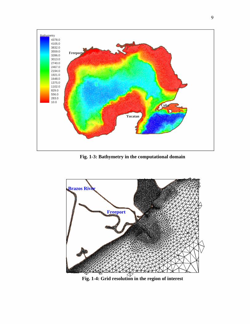
9

Bathymetry

10.0283.0556.0829.01102.01375.01648.01921.02194.02467.02740.03013.03286.03559.03832.04105.04378.0

Cuba

Yucatan

Freeport

Fig. 1-3: Bathymetry in the computational domain

Brazos River

Freeport

Fig. 1-4: Grid resolution in the region of interest

10

Fig. 1-5: Bathymetry in the area of interest

1.5 Outline

The thesis consists of 7 sections. Section 1 consists of motivation, approach, study

area, general procedure used in the thesis and outline. ADCIRC model and its

components, which are related to this thesis, constitute section 2. SLOSH model, its

history and methodology are described in section 3. Section 4 gives some insight into the

EST method. The implementation of ADCIRC and EST to the study area is further

described in section 5. The comparisons of ADCIRC/EST results with SLOSH model are

given in section 6. Section 7 consists of conclusions.

11

2 ADCIRC: MODEL DESCRIPTION

This section is divided into four parts. First part sheds light on ADCIRC model.

The other three parts discuss components of the model relevant to this thesis like tidal

forcing, bottom friction and wind forcing.

2.1 ADCIRC Model

Water-surface elevations and currents for both tides and storm events are obtained

from the large-domain long wave hydrodynamic model ADCIRC (Advanced Circulation

model; Luettich et al, 1992). ADCIRC is a finite element (FEM) code that makes use of

the Generalized Wave Continuity Equation (GWCE) for improved stability and

efficiency over other FEM hydrodynamic codes. Included within the code are features

that allow the user to include tidal and atmospheric forcing in the computations. Wind

can be input in a variety of different formats and could be derived from any source that

the user has available. The model was developed as a family of two- and three-

dimensional codes with the capability of:

a. Simulating tidal circulation and storm surge propagation over large computational

domains while simultaneously providing high resolution in areas of complex

shoreline and bathymetry. The targeted areas of interest include continental

shelves, near shore areas, and estuaries.

b. Representing all pertinent physics of the three-dimensional equations of motion.

These include tidal potential, Coriolis, baroclinic and all nonlinear terms of the

governing equations.

12

c. Providing accurate and efficient computations over time periods ranging from

months to years.

The 2-dimensional, Depth Integrated (2DDI) model formulation begins with the

depth-averaged shallow-water equations for conservation of mass and momentum subject

to incompressibility and hydrostatic pressure approximations. The Boussinesq

approximation, where density is considered constant in all terms but the gravity term of

the momentum equation, is also incorporated in the model. Using the standard quadratic

parameterization for bottom stress and omitting baroclinic terms and lateral diffusion and

dispersion, the following set of conservation statements in primitive, non-conservative

form and expressed in a spherical coordinate system are incorporated in the model

(Flather 1988; Kolar et al. 1994):

( cos1 [ ] 0 (1)cos

tan1 1 [ U ]cos

1 [ ( )] * cos

UVUHt R

U U UU V f VR Rt R

Pg UHR

s so o

φζφ λ φ

φφ λ φ

τ λζ η τρ ρφ λ

∂∂ ∂+ + =∂ ∂ ∂

∂ ∂ ∂+ + − + =∂ ∂ ∂

∂− + − + −∂ (2)

tan1 1 [ ]cos

1 [ ( )] * (3)cos

V V VU V U f VR Rt R

Pg VHR

s so o

φφ λ φ

τ φζ η τρ ρφ λ

∂ ∂ ∂+ + − + =∂ ∂ ∂

∂− + − + −∂

where :

ζ = free surface elevation relative to the geoid,

13

U, V = depth-averaged horizontal velocities,

H = ζ + h = total depth of water column,

h = bathymetric depth relative to the geoid,

f = 2 Ω sinφ = Coriolis force,

Ω = angular speed of the Earth,

φ = latitude in degrees,

λ = longitude in degrees,

Ps = atmospheric pressure at the free surface,

g = acceleration due to gravity,

η = effective Newtonian equilibrium tide potential,

oρ = reference density of water,

α = effective Earth elasticity factor,

,s sλ φτ τ = applied free-surface stress,

*τ = Cf (U2 + V2)1/2/H, bottom shear stress,

fC = bottom friction coefficient,

R = radius of Earth,

t = time.

In order to overcome general stability problems encountered when finite

element models depend upon the direct solution of these primitive forms of the governing

equations, the ADCIRC code was developed around the Generalized Wave Continuity

Equation (GWCE). Combining a time-differentiated form of the momentum equations

14

yields this form of the primitive equations. With the inclusion of a simple eddy viscosity

model for closure (Kolar and Gray 1994), the GWCE in Spherical coordinates takes the

form:

202

0 0

( ) ( cos ) tan1 1 ( )cos cos

2 sin ( ( ) )cos

( ) ( cos ) tan1 1[ ( ) 2 sin ]cos

1 [ ( ( )

S

HUV HUVUVH Rt R Rt

HHV g HU HUR

HVV HVVUUH HUR RR

H gR R

Pso o

Ps

λ

φδ ζ ζ φφ λ φ λ φδ

ω φ ζ αηφ λ

φ φω φφ φ λ φ

ζ αηφ λ

τρ ρ

ρ

τ

τ τ

∂ ∂∂ ∂+ − + −∂ ∂ ∂ ∂

∂− − + − + + − −∂

∂ ∂∂− + + +∂ ∂ ∂

∂ ∂− − +∂ ∂

⎡ ⎤⎣ ⎦

⎡ ⎤⎢ ⎥⎣ ⎦

0

0

) ( * ) ]

[ tan ] [ tan ] 0

sHV

VH VHR Rt

o oφ

τ τ

φ φ

τρ

τ

+ − −

∂− − =∂

(4)

The ADCIRC-2DDI model solves the GWCE (Equation (4)) in conjunction with

the primitive momentum equations given in Equations (2) and (3). The equations are

solved using a FEM grid, made up of linear triangular elements (only three nodes per

element). The model domain can be as extensive as an entire ocean basin, or more

localized, as in the case of a small bay or estuary. The numerical solution of the

governing equations presented above follows a two-step procedure in ADCIRC code.

First, the GWCE (Equation (4)) is solved. The linear terms in the GWCE are discretized

using a Galerkin weighted residual, three time level, and implicit scheme. The non-linear

terms, along with Coriolis forcing, atmospheric forcing and tidal potential are solved

15

explicitly (Westerink et al. 1993). The explicit formulation of these terms has the

advantage that the solution depends only upon the previous time step. On the other hand,

the implicit terms depend upon the solution of a system of equations, arranged in a

banded matrix.

The second step in the solution of the governing equations, after solving the

GWCE, is to solve the momentum equations (Eq. (2) and (3)). Most of the terms of the

momentum equations are handled in a Crank-Nicholson, two-time level, and implicit

discretization scheme. The explicit terms in the momentum equations are the *τ terms,

the convective terms and the eddy viscosity terms.

The available boundary conditions used in ADCIRC include:

specified elevation (harmonic tidal constituents or time series)

specified normal flow (harmonic tidal constituents or time series)

zero normal flow

slip or no slip conditions for velocity

external barrier overflow out of the domain

internal barrier overflow between sections of the domain

surface stress (wind and/or wave radiation stress)

atmospheric pressure

outward radiation of waves (Sommerfield condition)

Those used in the model are described in section 5.4

ADCIRC can be forced with:

elevation boundary conditions

normal flow boundary conditions

16

surface stress boundary conditions

earth load/self attraction tide

A feature of ADCIRC that makes its application particularly useful in storm surge

modeling of bays along the Texas Gulf coast is the capability of wetting and drying in the

computational cells. Most of the coastal basins that make up the estuaries along the Texas

Gulf coast are very shallow, with depths that are often no more than a meter. In addition

to the shallow bay depths, the topography of coastal lands is that of flat coastal plains,

with very gentle slopes. The barrier islands in Freeport are just a few meters above mean

water level. During extreme meteorological events like hurricanes, it is possible that

shallow areas may become dry from “blow down” (due to water being driven from the

area by storm winds). On the other hand, the surge during a storm can cause extensive

inland coastal flooding as is evident historically in all large storms affecting the Freeport

area over the time period considered in this study.

An element based technique for wetting/drying was developed for implementation

in ADCIRC. Conceptually, the algorithm assumes removable barriers exist along the

sides of all triangular elements of the grid. Nodes of the elements are designated as “dry”

nodes, “interface” nodes, and “wet” nodes. All elements connected to a dry node are

assumed to have barriers in place such that there is no flow through the element, i.e. a dry

element. An element connected to all wet nodes is a wet element and is included in the

full flow domain. Interface nodes connect wet and dry elements. Boundaries connecting

interface nodes are considered as standard land boundary nodes at which the water level

rises and falls against the element barrier.

17

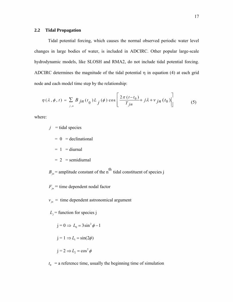
2.2 Tidal Propagation

Tidal potential forcing, which causes the normal observed periodic water level

changes in large bodies of water, is included in ADCIRC. Other popular large-scale

hydrodynamic models, like SLOSH and RMA2, do not include tidal potential forcing.

ADCIRC determines the magnitude of the tidal potential η in equation (4) at each grid

node and each model time step by the relationship:

,

000

2 ( )( , , ) ( ) ( ) cos ( )

j n

t tt t L

T jnB j v tjn jnj

πη λ φ φ λ−

=⎡ ⎤

+ +⎢ ⎥⎢ ⎥⎣ ⎦

∑ (5)

where:

j = tidal species

= 0 = declinational

= 1 = diurnal

= 2 = semidiurnal

jnB = amplitude constant of the nth tidal constituent of species j

jnF = time dependent nodal factor

jnv = time dependent astronomical argument

jL = function for species j

j = 0 ⇒ 20 3sin 1L φ= −

j = 1 ⇒ 1 sin(2 )L φ=

j = 2 ⇒ 22 cosL φ=

0t = a reference time, usually the beginning time of simulation

18

jnT = period of constituent n of species j

The values of f ( jnB ) and ν for the constituents used for the tidal potential computations

are determined for the specific time that a model run begins using Le Provost database

(Westerink, J.J. et al, 1993). LeProvost database (Le Provost et al, 1994) is an atlas of the

main components of the tides and has been produced on the basis of a finite element

hydrodynamic model, with the aim of offering the scientific community, using satellite

altimetric data, a prediction of the tidal contribution to sea surface height variations under

the ground tracks of the satellite that is totally independent of altimetric variation. Eight

constituents, M2, S2, N2, K2, 2N2, K1, O1, and Q1 have been simulated. Five secondary

constituents: Mu2, Nu2, L2, T2, and P1, required to insure a priori correct predictions, have

been deduced by admittance. The admittance is assumed to be a slowly varying function

of frequency so that the admittance of the major constituents can be used for determining

the response at nearby frequencies for the secondary constituents.

The accuracy and precision of these solutions have been estimated by reference

to the harmonic constituents’ data set available from analysis of the entire collection of

the pelagic, plateau and coastal observations made to date, and archived. Over the deep

oceans these solutions fit the observations to within a few centimeters for the larger

components: M2, S2, K1, O1, and a few millimeters for the others. Over the continental

shelves the differences are larger, because of the increase in the magnitude of the tidal

waves, but the flexibility offered by the finite element technique to refine the

discretization mesh of the model over the shallow seas enables detailed cotidal maps to

be produced along the coasts. Note that tidal potential was not used during the simulation

19

of tropical storms. Tides were combined after the simulations during the frequency

analysis.

2.3 Bottom Stress

Bottom stress in the 2DDI version of ADCIRC is generally expressed as:

*bx Uτ τ= and *

by Vτ τ=

Depending on the form used for τ* the result is either a linear, quadratic or hybrid

function of depth-averaged velocity. For most coastal applications, quadratic friction

should be used with a drag coefficient, Cf ∼ 0.0025. In very shallow water, hybrid friction

may be useful with Cfmin ∼ 0.0025, particularly when wetting and drying is included since

this expression becomes highly dissipative as the water depth becomes small. Linear

friction is primarily useful for model testing or when a totally linear model run is desired.

In this case the magnitude of τ* should be consistent (at least in order of magnitude) with

a value that would have been computed using the quadratic friction expression and not

with the value of Cf that would normally be used in the quadratic expression. The

description of formulation based on the form of τ* is given here.

Linear friction: τ* = Cf

where Cf = constant in time (may vary with space), read in model as input, unit s-1

Quadratic friction: ( )

HVUC f 2

122

*+

≡τ

where Cf = constant in time (may vary with space), read in model as input

H = water depth

20

Hybrid friction: ( )

HVUC f 2

122

*+

≡τ

where θ

γθ

⎥⎥⎦

⎤

⎢⎢⎣

⎡⎟⎠⎞

⎜⎝⎛+=

HHCC break

ff 1min

and Cfmin, Hbreak, ϑ, γ are constant in time and are read in as model input

In the hybrid friction relationship Cf approaches Cfmin in deep water, (H> Hbreak),

and approaches γ

⎟⎠

⎞⎜⎝

⎛H

HC breakf min in shallow water, (H < Hbreak ). The exponent ϑ

determines how rapidly Cf approaches each asymptotic limit and γ determines how

rapidly the friction coefficient increases as water depth decreases. If H

ngC

breakf γ

2

min = and γ

= 1/3, where g is the gravitational constant and n is the Manning Coefficient, the hybrid

friction will have a Manning equation frictional behavior for H < Hbreak.

2.4 Wind Forcing

In addition to the capability for tidal forcing within ADCIRC, there are provisions

to input atmospheric and wind forcing information into the simulations. Several formats

for the wind data are supported, including a fleet numeric and National Weather Service

(NWS) wind file format. For this study, the Planetary Boundary Layer (PBL) model

(Cardone et al. 1992) supplies the atmospheric forcing information. This model was

developed to simulate hurricane generated wind fields using basic characteristics about a

particular storm that can be easily retrieved from sources such as NWS archives of past

hurricanes.

21

The input data to the model consists of location of the eye of the hurricane

(latitude and longitude) in degrees, wind speed and pressure measured at the eye for 6-

hour intervals. Such data are available for all the storms. A sample input data for

Hurricane Claudette (2003) is shown in Table 2-1.

Table 2-1: Input data for Hurricane Claudette (2003)

Time (Day.

Hour) Latitude Longitude

Maximum

wind speed

(knots)

Eye Pressure

(mm of Hg)

15.03 27.8 -94 70 988

15.09 28 -95.1 75 982

15.15 28.5 -96.1 75 983

15.21 28.6 -97.5 65 989

There are five simple parameters to describe the strength, size, and motion of a

model storm; the parameters are: (1) Latitude: Normally the latitude of the storm's

landfall; if the storm does not landfall, the latitude of a point of interest on the coast. The

storm surge is only mildly sensitive to this parameter and varies by less than 10 percent

between latitudes 15° and 45°, all other parameters being the same. (2) Radius of

maximum winds: The distance from the storm center to the maximum wind of the storm.

This distance is not dependent on storm motion, and for any given time it is assumed to

be the same in all directions. This parameter controls the horizontal extent of the surge on

the coast. If only the value of the peak surge on the coast is desired then the accuracy of

22

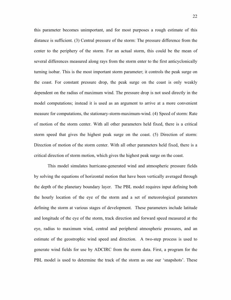
this parameter becomes unimportant, and for most purposes a rough estimate of this

distance is sufficient. (3) Central pressure of the storm: The pressure difference from the

center to the periphery of the storm. For an actual storm, this could be the mean of

several differences measured along rays from the storm enter to the first anticyclonically

turning isobar. This is the most important storm parameter; it controls the peak surge on

the coast. For constant pressure drop, the peak surge on the coast is only weakly

dependent on the radius of maximum wind. The pressure drop is not used directly in the

model computations; instead it is used as an argument to arrive at a more convenient

measure for computations, the stationary-storm-maximum-wind. (4) Speed of storm: Rate

of motion of the storm center. With all other parameters held fixed, there is a critical

storm speed that gives the highest peak surge on the coast. (5) Direction of storm:

Direction of motion of the storm center. With all other parameters held fixed, there is a

critical direction of storm motion, which gives the highest peak surge on the coast.

This model simulates hurricane-generated wind and atmospheric pressure fields

by solving the equations of horizontal motion that have been vertically averaged through

the depth of the planetary boundary layer. The PBL model requires input defining both

the hourly location of the eye of the storm and a set of meteorological parameters

defining the storm at various stages of development. These parameters include latitude

and longitude of the eye of the storm, track direction and forward speed measured at the

eye, radius to maximum wind, central and peripheral atmospheric pressures, and an

estimate of the geostrophic wind speed and direction. A two-step process is used to

generate wind fields for use by ADCIRC from the storm data. First, a program for the

PBL model is used to determine the track of the storm as one our ‘snapshots’. These

23

snapshot data include the radius of maximum wind, which is approximated using a

nomograph that incorporates the maximum wind speed and atmospheric pressure

anomaly (Jelesnianski and Taylor, 1973), which is shown in Fig. 2-1. In the second step,

the PBL model computes the wind field and pressure field of the hurricane over the

relevant areas of the Gulf of Mexico.

Fig. 2-1: Nomograph from Jelesnianski and Taylor (1973) used to derive radius of maximum winds from given maximum surface winds (long term average, no gusts)

2.4.1 PBL

The PBL (Planetary Boundary layer) is a method for specifying the surface wind

field in hurricanes over the ocean by applying a dynamical-numerical model in

24

hurricanes. The method, requiring as input only a description of the surface pressure field

and specification of storm motion and latitude, has been used to model the surface wind

field.

The PBL model solves for the surface wind stress and barometric pressure

distribution. Wind speeds are computed in the model and then converted to surface wind

stress. The PBL model solves the equations of horizontal motion that have been averaged

through the depth of the atmospheric boundary layer, following the work of Chow (1971)

. Written in general coordinate system fixed to the earth these equations can be expressed

as:

( ) ( )1 DH

CdV f k V p K V V Vdt hρ

+ × = − ∇ + ∇ ⋅ ∇ −r ur ur ur ur

(6)

where

VVtV

dtVd

∇⋅+∂∂

= (7)

and

V = vertically averaged horizontal velocity,

f = Coriolis force parameter,

kr

= unit vector in the vertical direction,

ρ = mean air density,

p = barometric pressure,

KH = horizontal eddy viscosity coefficient,

CD = drag coefficient,

h = depth of the boundary layer.

25

It is assumed that the vertical advection of momentum is small compared to the

horizontal advection and can be neglected and that shearing stress vanishes at the top of

the PBL. In addition to the storm winds, the PBL model generates a pressure field. The

pressure field is axisymmetric and is defined by exponential law which expresses Pc, the

pressure at a particular location in the storm, as:

rR

eyec

p

pePP−

∆+= (8)

where,

Peye = the central low pressure at the eye of the storm,

p∆ = P- Peye, where P is the normal background pressure (∼ 1013 mb),

Rp = scale radius, equivalent to the radius of maximum winds,

r = radial distance from the eye.

These equations are solved using a finite difference formulation, which utilizes a

nested rectangular mesh for computations. The computational grid is a rectangular nested

grid system consisting of five nests. An example of this type of mesh is shown in Fig.

2-2, where a single quadrant of the complete numerical grid is shown. The grid moves

with the storm, therefore the eye of the hurricane is always centered about the point

indicated as origin.

26

Fig. 2-2: Nested grid system used for hurricane wind computation

The PBL model produces a consistent description of the vertically integrated

wind, the surface drag and the wind speed and direction at anemometer height in a

moving hurricane with asymmetric horizontal wind distribution over water, with the

27

strongest winds occurring at the right-hand side of the storm, when facing the direction of

travel of storm. The formulation of the model includes momentum, heat, and moisture

flux. Equilibrium PBL theory is used to extend the surface wind description to terrain of

specified roughness.

The final surface wind stress output of the PBL model is determined from the

computed wind speeds using the relationships:

φφ

ρρ

ρτ VVC

o

airD

o

s = (9)

and

λλ

ρρ

ρτ VVC

o

airD

o

s = (10)

where,

τφ, τλ = the surface stresses applied in the φ and λ directions

ρair/ρo = density ration of air and seawater (∼ 0.001293)

V = absolute magnitude of the wind velocity

φV , λV = components of wind velocity in φ and λ directions

CD = 0.001*(0.75+0.67* V ) frictional drag coefficient

φ, λ = directions

A plot of the wind shear stress in a well-developed hurricane is shown in Fig.

2-3, where it is shown that the greatest winds in this case occur north-east of the eye of

this north-westerly moving storm.

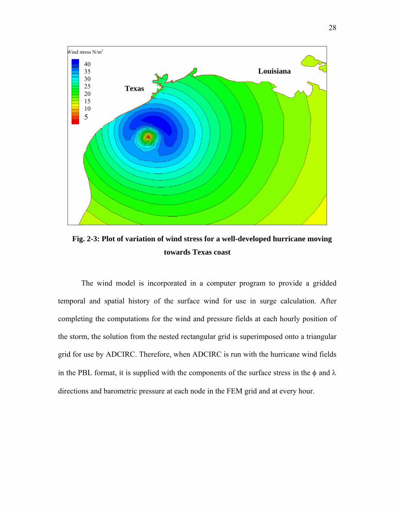
28

Texas

Louisiana

Wind stress N/m2

40 35 30 25 20 15 10 5

Fig. 2-3: Plot of variation of wind stress for a well-developed hurricane moving

towards Texas coast

The wind model is incorporated in a computer program to provide a gridded

temporal and spatial history of the surface wind for use in surge calculation. After

completing the computations for the wind and pressure fields at each hourly position of

the storm, the solution from the nested rectangular grid is superimposed onto a triangular

grid for use by ADCIRC. Therefore, when ADCIRC is run with the hurricane wind fields

in the PBL format, it is supplied with the components of the surface stress in the φ and λ

directions and barometric pressure at each node in the FEM grid and at every hour.

29

3 SLOSH

A numerical-dynamic, tropical storm surge model, was developed for real-time

forecasting of hurricane storm surges on continental shelves, across inland water bodies,

along coastlines, and for inland routing of water – either from the sea or from inland

water bodies. The most valuable application of SLOSH (Sea, Lake, and Overland Surges

from Hurricanes) was in the design of evacuation plans for various communities.

SLOSH is a two-dimensional finite difference code, which has been programmed

to utilize a variety of curvilinear grid formats, such as polar, elliptical, and hyperbolic

(Jelesnianski 1973). The full length of East coast and Gulf coast of the United States is

broken down into several regional grids, or model “basins”. Each basin in turn is centered

about a major bay, inlet or population center. The individual SLOSH basins that are used

by NWS are shown in Fig. 3-1. An example of one of these model basins is shown in the

grid no. 31 used for Galveston Bay in Fig. 3-2. The results from this grid have been used

in this thesis for comparison purposes.

3.1 Development of SLOSH

The National Weather Service (NWS) began its efforts in hurricane storm surge

modeling with a relatively simple model referred to as SPLASH (Special Program to List

the Amplitude of Storm surges from Hurricanes). This model, like several other simple

models for computing storm surge, was restricted to a continental shelf only, with the

coastline acting as an artificial vertical wall. No flow through this wall was permitted.

Such a model cannot consider inundation across terrain or surges across inland water

bodies (Jelesnianski, 1972; Wanstrath and Reid, 1976). An earlier shelf model by Bodine

30

(1971) was even more restricted. His model required computations carried out on only

one seaward line from the coast. Also the storm track was restricted to being nearly

perpendicular to the coastline.

The National Weather Service (NWS) embarked on an effort to develop a more

comprehensive model to forecast storm surges, which incorporated features not possible

with SPLASH. This follow-on model called SLOSH, uses a curvilinear grid system to

allow greater resolution in the area of forecast interest, computes surges over bays and

estuaries, retains some non-linear terms in the equation of motion, and allows sub-grid

scale features such as channels, barriers, and flow of surge up the rivers. More recently

the model has been used to delineate coastal areas susceptible to hurricane storm surge

flooding.

A curvilinear grid system overcomes many of the problems associated with

specifying boundary conditions encountered with earlier models. Instead of limiting an

invariant fine mesh to a small region or small basin, the SLOSH model’s coordinate

system begins as fine mesh in the limited area nearest to the pole point of the grid and

stretches continuously to a coarse mesh at distant boundaries of a large basin. The

geographical area covered by the entire grid is large and there is detailed description over

the fine-mesh region. Moreover, in many cases simple boundary conditions are sufficient

(Jelesnianski et al, 1992).

31

Fig. 3-1: SLOSH model basins for the East and Gulf coastlines of the U.S. (Jelesnianski et al, 1992)

32

Fig. 3-2: SLOSH model basin for Galveston Bay (Jelesnianski et al, 1992)

33

3.2 SLOSH Methodology

The transport equations of motion on a Cartesian frame of reference used are:

( ) ( )( ) ( )

( ) ( )( ) ( )

o or i r i

o or i r i

i

i

r

r

h h h hU g D h f AV AU C x C yB Bt x y

h h h hV g D h f AU AV C y C xB Bt y x

h U Vt x y

τ τ

τ τ

⎡ ⎤∂ − ∂ −∂= − + − + + + −⎢ ⎥∂ ∂ ∂⎣ ⎦

⎡ ⎤∂ − ∂ −∂= − + + − − + +⎢ ⎥∂ ∂ ∂⎣ ⎦

∂ ∂ ∂= − −

∂ ∂ ∂

(11)

where:

U, V = components of transport

g = gravitational constant

D = depth of quiescent water relative to a common datum

h = height of water above datum

ho = hydrostatic water height

f = Coriolis parameter

xτ,yτ = components of surface wind stress

Ar,..Br,.Ci = bottom stress terms

The SLOSH model incorporates finite amplitude effects but not advective terms

in the equations of motion. It uses time-history bottom stress (Platzman, 1963;

Jelesnianski, 1967), corrected for finite amplitude effects. Overtopping of barrier

systems, levees and roads, is incorporated. Also, simply turning squares on and off as

water inundates or recedes permits inland inundation. Astronomical tide is ignored except

for superposition onto the computed surge; it is difficult to phase storm landfall and

astronomical tide. A small error in time on track positions will invalidate computations

with astronomical tide.

34

Besides the hydrodynamic model, the most significant part of SLOSH is the wind

model that is used to generate hurricane wind fields using simple time-dependent storm

data. The storm data required by SLOSH are storm position and central pressure at six-

hour intervals. Each model basin is calibrated separately by a single historic event

through the use of three empirical coefficients in the model. These tuning coefficients are

eddy viscosity, bottom friction factor, and wind drag. They are set to the same value at

each node of the model basin, and these values are usually determined by a best-fit

approximation. After the initial calibration of the model basin, no additional tuning is

made for further model runs.

3.3 SLOSH Output

The final output of the SLOSH model runs gives both local information at

selected sites in the grid, and global output for the entire modeled domain. Local, time-

dependent data are collected from as many as 60 individual stations. These time histories

present the surge elevation, wind speed and wind direction every 10 minutes of simulated

time. In addition to the model station output, SLOSH outputs global (values for each

node in the grid) surge elevations. The global data is output at three-hour intervals up to

the closest approach of the storm, and then every two hours, up until nine hours beyond

the closest approach.

There are other factors also that can have a significant influence on the total water

level elevation during a storm. In coastal regions, the action of breaking waves can create

a quasi-steady-state, long period “set-up” (if not set-down) whereby the original storm

surge is altered. This wave action can affect bottom stress in shallow waters. Also, exotic

effects occur such as an increase of density from suspended sand particles. Along coastal

35

regions, during passage of a tropical storm and onset of inundation, the totality of wind-

wave effects on surge is now well understood or even well observed. Many theoretical

studies of an idealized and piecemeal nature, as well as idealized wave tank experiments,

have been made. It is not sufficient to correct a computed surge for one or more long-

term interactions. Accordingly, the SLOSH model lumps the long-term interactions into

an ad hoc generalized calibration to observed surge data generated by a multitude of

historical storms: that is, the short term action from wind waves is absent but crude

approximations for the long term effects may be present. The SLOSH model does give an

indication of inland flooding but not the pulsating action of wind waves, such as short-

term, periodic, sheet flow over barriers (Jelesnianski et al, 1992).

36

4 THE EMPIRICAL SIMULATION TECHNIQUE

The Empirical Simulation Technique (EST) is a procedure for simulating multiple

life-cycle sequences of non-deterministic multi-parameter systems such as storm events

and their corresponding environmental impacts. Essentially, it is a "Bootstrap"

resampling-with-replacement, interpolation, and subsequent smoothing technique in

which random sampling of a finite length database is used to generate a larger database

(Borgman et al. 1992). The only assumption is that future events will be statistically

similar in magnitude and frequency to past events. As stated above, EST is a generalized

procedure applicable to any cyclic or frequency-related phenomena (Scheffner et al,

1999). For example, if one can parameterize storm events as well as obtain or simulate

corresponding historical impacts for these events, EST could be used to investigate life-

cycle scenarios of storm conditions. The EST begins with an analysis of historical events

that have impacted a specific locale. The selected database of events (the training set) is

then parameterized to define the characteristics of the event. The interdependence of

parameters is computed directly from the respective parameter interdependencies

contained in the historic data. In this manner, probabilities are site-specific; do not

depend on fixed parametric relationships or assumed joint probability distributions. The

impacts of events may be known or may be simulated by other models (e.g., hurricane

events can be characterized by parameters such as central pressure, forward speed, etc.

and their impact may be simulated with appropriate hydrodynamic and storm wind

models). Parameters that describe an event, i.e., a storm in this discussion, are referred to

as input parameters or input vectors. Response parameters or response vectors define

event-related impacts such as storm surge elevation, inundation, shoreline and dune

37

erosion, etc. These input parameters and response parameters are then used as a basis for

generating life-cycle simulations of hurricane activity with corresponding impacts.

The descriptive characteristics of the storm event with respect to the specific

location of interest are determined by the input parameters or input vectors. For tropical

storms these input parameters are studied at the point when the eye of the hurricane is

closest to the station of interest. These vectors are defined as:

1) tidal phase during the event, with 1.0 corresponding to high water slack,

0.0 MSL at maximum ebb, -1.0 low water slack, these represent relative

values that are defined for each station

2) radius of maximum wind for the hurricane when the eye is closest to the

hurricane in nautical miles.

3) minimum distance from the eye of the storm to the location of interest in

nautical miles.

4) pressure at the hurricane eye in millibars (mb)

5) wind speed in the hurricane at the instant of eye hitting the coast,

measured in knots.

6) direction of forward propagation of the eye of the hurricane in knots.

7) tidal range during the event: with spring, neap or mid tide conditions.

The maximum storm surge elevation reached at specified gauge locations is

defined as the response vector of the storm at that location. The specified response vector

for this study was determined by simulating the specific storm event via the ADCIRC

hydrodynamic model using the computational domain shown in Fig. 1-2. The output

vector(s) represents the environmental response to the storm. This response is defined at

location X and is a direct consequence of the storm via the storm parameter values

38

defined at the point of nearest proximity of the storm eye to point X. For the case of

stage-frequency analyses, maximum surge is assumed to occur when the eye of the storm

is nearest to location X.

4.1 Storm Consistency with Past Events

The first major requirement for the use of EST is that future events will be

statistically similar to past events. This criterion is maintained by insuring that the input

vectors for simulated events are similar to those of past events and the input vectors have

similar joint probabilities to those historical events of the training set. For example, a

hurricane with a large central pressure deficit and low maximum winds is not a realistic

event – the two parameters are not independent although their precise dependency is

unknown. The simulation of realistic events is accounted for in the nearest-neighbor

interpolation-bootstrap-resampling technique developed by Borgman (Scheffner, et al.

1999 and Borgman, et al. 1992). By using the training set as a basis of for defining future

events, unrealistic events are not included in the life cycle of events generated by the

EST. Events that are output by EST are similar to those in the training set with some

degree of variability from the historic/historically based events. This variability is a

function of the nearest neighbor: therefore the deviation from historic conditions is

limited to natural variability of the system.

The basic technique can be described as follows. Let X1, X2, X3, . . . Xa be n

independent, identically distributed random vectors (historic storm events) each having

two components [Xi=xi(1),xi(2); I =1,n]. If there are no hypothetical events, each

event Xi has a probability pi of l/n. If one storm event is used to generate two

hypothetical events, then the original storm and each of the two perturbations are

39

assigned a probability of one-third of l/n. A cumulative probability relationship can be

developed in which each storm event of the total training set is assigned a segment of the

total probability of 0.0 to 1.0. Therefore each event occupies a fixed portion of the 0.0 to

1.0 cumulative probability spaces according to the total number of events in the training

set. A random number from 0 to 1 is then used to identify a storm event from the total

storm training set population. The procedure is equivalent to drawing and replacing a

random sample from the full storm event population.

The EST is not simply a resampling of historical events technique, but rather an

approach intended to simulate the vector distribution contained in the training set data

base population. The EST approach is to select a sample storm based on a random

number selection from 0 to 1 and then performs a random walk from the event Xi with n

number of response vectors to the nearest neighbor vectors. The walk is based on

independent uniform random numbers on (-1,1) and has the effect of simulating

responses that are not identical to the historical events but are similar to events, which

have historically occurred. However it is important to point out that it is possible that the

response value of water surface elevation (i.e. tide plus surge) may be greater than the

greatest value in the total training set or it could be smaller than the smallest of the

training set.

The process can be summarized as follows. Select a specific storm event from the

training set and proceed to the location in multidimensional input vector space

corresponding to that event. From that location, perform a nearest neighbor random walk

to define a new set of input vectors. This new input vector defines a new storm, similar to

the original storm but with some variability in parameters.

40

4.2 Storm Event Frequency

The second criteria to be satisfied is that the number of storm events selected per

year must be statistically similar to the number of historical events that have occurred at

the area of concern. Given the mean frequency of storm events for a particular region, a

Poisson distribution is used to determine the average number of expected events in a

given year. For example, a Poisson distribution can be written in the following form:

!);Pr( ses

s λλλ−

= (12)

for s=0,1,2,3… The probability Pr(s;λ) defines the probability of having s events per year

where λ is the historically based number of events per year. In the present study,

historical data were used to define λ as:

λ = 0.2307 (27 historical events/117 years or one event every 4.33 years)

Output from the EST program is N repetitions of T years of simulated storm event

responses. For this study, 500 repetitions, N, of a 200 year sequence, T, of storm activity

are used. It is from the responses of those 500 life cycle simulations that frequency-of-

occurrence relationships are computed. Because EST output is of the form of multiple

time–series simulations, post processing of output yields mean value frequency

relationships with definable error estimates. The computational procedure followed is

based on the generation of a probability distribution function corresponding to each of the

T-year of simulated data. In the following section, the approach adopted for using these

storms to develop frequency-of-occurrence relationships is given.

41

4.3 Risk-Based Frequency Analysis

The primary justification for applying the EST to a specific project is to generate

risk-based frequency information relating to effectiveness and cost of the project with the

level of protection provided. The multiple life-cycle simulations produced by EST can be

used for developing design criteria in two approaches. In the first, the actual time series

are input to an economics based model that computes couple storm inundation, structure

response, and associated economics. The model internally computes variability

associated with the risk-based design. The other application is the post processing of

multiple time-series to generate single-response frequency relationships and associated

variability.

4.4 Frequency-of-Occurrence Relationships

Estimates of frequency-of-occurrence begin with the calculation of a probability

distribution function (pdf) for the response vector of interest. Let X1, X2, X3, . . . , Xn be

n independent, identically distributed, random response variables with a cumulative pdf

given by

Fx (x) = Pr [X < x] (13)

where Pr[X<x] represents the probability that the random variable X is less than or equal

to some value x, and Fx(x) is the cumulative probability density function ranging from 0.0

to 1.0. The problem is to estimate the value of Fx without introducing some parametric

relationship for probability. The following procedure is adopted because it makes use of

the probability laws defined by the data and does not incorporate any prior assumptions

concerning the probability relationship.

42

Assuming a set of n observations of data, the n values of x are first ranked in

order of increasing size. In the following analysis, the parentheses surrounding the

subscript indicate that the data have been rank-ordered. The value x(1) is the smallest in

the series and x(n) represents the largest value. Let r denote the rank of the value x(r)

such that rank r = 1 is the smallest and rank r = n is the largest.

An empirical estimate of Fx(x(r)), denoted by Fx(x(r)), is given by Gumbel (1954)

(See also Borgman and Scheffner (1991) and Scheffner and Borgman (1992)) as:

)1()( )( += n

rxF rχ (14)

for x(r), r = 1, 2, 3, . . ., n. This form of estimate allows for future values of x to be less

than the smallest observation x(1) with a cumulative pdf of 1/(n+1), and to be larger than

the largest values with cumulative pdf of n/(n+1).

The cumulative pdf as defined by Equation (14) is applied to develop stage-

frequency relationships as follows. Consider that the cumulative probability for an n-

year return period storm can be written as

nnF 11)( −= (15)

where F(n) is the simulated cumulative pdf for an event with a return period of n years.

Frequency-of-occurrence relationships are obtained by linearly interpolating a stage from

Equation (14) corresponding to the pdf associated with the return period calculated by

Equation (15).

Equations (14) and (15) are applied to each of the N-repetitions of T-years of

storm events simulated via the EST. Therefore, there are N frequency-of-occurrence

relationships generated. From these results, the standard deviation is determined to

43

provide an estimate of the variability of the result. The standard deviation is computed

for each return period as:

2(1 / ) ( ) ]

1

NN x xnn

σ−

∑= −=

⎡ ⎤⎢ ⎥⎣ ⎦ (16)

where x is the mean value of x.

44

5 PROJECT IMPLEMENTATION

The model as stated before required the generation of finite element grid and

application of appropriate boundary conditions in order to simulate tides and coupling

with the wind model PBL, to simulate hurricanes and tropical storms. The process

required the following tasks:

1. Obtaining Coastline

2. Obtaining Bathymetry

3. Grid generation

4. Boundary conditions

5. Tidal verification

6. Storm verification, simulation and entry into database

7. EST analysis

5.1 Coastline

The coastline is required to define the extents of the model domain. This will

become the boundary of the computational mesh. The coastline around our area of

interest as well as the ocean defines the domain. The coastline for this purpose is obtained

in digital format from GEODAS and NOAA databases. The coastline is in the form of

World Vector Shoreline subset at 1:1million resolution (altered) format. Since the

obtained coastline was ragged in nature, it was smoothened before being used for grid

generation.

45

5.2 Bathymetry

The bathymetry in the Gulf of Mexico varies dramatically, as is illustrated in the

Fig. 1-3. Bathymetric data in most of the Gulf was obtained from the grid developed by

Scheffner et al. (2003), GeoDas (a database developed by National Oceanic and

Atmospheric Administration, NOAA), USACE surveys, surveys conducted by Texas

A&M University in the area of interest, and USGS terrain data. The terrain data was in

the form of 30-meter grid digital elevation models (DEM). These data are based on the

USGS 7.5 minute x 7.5-minute quads maps and are interpolated from 5-foot elevation

contours.

5.3 Grid Generation

The grid was generated as a combination of finite element grid developed by

Scheffner et al. (2003) and modified in the area of interest with details added. The grid in

the area of interest was developed using SMS (Surface Modeling System). To get a

mesh/grid with density radiating from the center of the Freeport channel, size functions in

SMS were used along with celerity and wavelength functions so that smaller elements are

obtained closer to the shore to correctly model the area of interest.

5.4 Boundary Conditions and Model Setup

Boundary conditions are imposed on the solutions of ordinary differential

equations and partial differential equations, to fit the solutions to the actual

problem.There are many kinds of possible boundary conditions, depending on the

formulation of the problem, number of variables involved, and (crucially) the

mathematical nature of the equation.

46

The boundary conditions used within ADCIRC for this study were:

• External boundary with no normal flow as an essential boundary condition and

no constraint on tangential flow. This is applied by zeroing the normal boundary

flux integral in the continuity equation and by zeroing the normal velocity in the

momentum equations. This boundary condition should satisfy no normal flow in

a global sense and no normal flow at each boundary node. This type of

boundary represents a mainland boundary with a strong no normal flow

condition and free tangential slip.

• Internal boundary with no normal flow treated as an essential boundary

condition and no constraint on the tangential flow. This is applied by zeroing

the normal boundary flux integral in the continuity equation and by zeroing the

normal velocity in the momentum equations. This boundary condition should

satisfy no normal flow in a global sense and no normal flow at each boundary

node. This type of boundary represents an island boundary with a strong normal

flow condition and free tangential slip.

• External boundary with non-zero normal flow as an essential boundary

condition and no constraint on the tangential flow. This is applied by specifying

the non-zero contribution to the normal boundary flux integral in the continuity

equation and by specifying the non-zero normal velocity in the momentum

equations. This boundary condition should correctly satisfy the flux balance in a

global sense and the normal flux at each boundary node. This type of boundary

represents a river inflow or open ocean boundary with a strong specified normal

flow condition and free tangential slip.

47

There are several other boundary conditions that can be applied in ADCIRC but

they were not needed for the present model. The model was “spun up” (started with

progressively increasing forcing such as tides or winds) from homogeneous initial

conditions using a time ramp to avoid problems with short period gravity modes and

vortex modes in the sub internal frequency range. A very smooth hyperbolic tangent

ramp function, which acts over approximately one day, was applied to both boundary

conditions and direct forcing functions. A 6-day spin-up was determined to be more than

adequate for all conditions of interest.

A time step of 6 sec was used for tidal propagation and a time step of 2 seconds

was used for storm simulation in order to accommodate the strong gradients associated

with strong winds for storm conditions. Using higher time steps resulted in oscillations

and long-term instabilities. The optimal time step was calculated based on Courant

number criteria. The Courant Number criteria is usually expressed in the one-dimensional

form as follows:

Courant number = xtv

∆∆

where:

∆x = nodal spacing

v = average linear velocity

∆t = incremental time step

The Courant Number constraints provide the necessary conditions for the finite

element mesh design and the selection of time steps in transport modeling. The Courant

Number constraint requires that the distance traveled by advection during one time step is

not larger than one spatial increment. Based on wave celerity, it ranged from 0.0025 to

48

0.82. Time weighing factors of 0.35, 0.30 and 0.35 were used in the GWCE (Generalized

Wave Continuity Equations). The parameter τ0 was set equal to –0.005 as this signals

ADCIRC to use 0.005 in deep water and 0.02 in shallow water, so that a balance is set

between the primitive continuity and wave equation portions of the GWCE equation.

Table 5-1: List of stations used for tidal verification

S. No Location Longitude ° Latitude °

1 Corpus Christi -97.38928 27.08113

2 Freeport Harbor -95.34277 28.95019

3 Sabine Pass -93.83873 29.68882

4 Galveston Bay entrance south jetty -94.69849 29.32304

5 Round Point Galveston Bay -94.78059 29.31827

6 Galveston Bay entrance -94.70587 29.34739

7 Bolivar Roads -94.78388 29.34029

8 Galveston (channel) (2) -94.78774 29.31305

9 Galveston Pleasure Pier -94.78747 29.28495

10 Galveston Channel -94.80136 29.31203

11 Jamaica Beach -95.00899 29.19919

12 Morgan Point -94.9766 29.6756

13 Clear Lake -95.06118 29.55583

14 Lynchburg Landing -95.09607 29.77917

15 San Luis Pass -95.12016 29.07968

49

5.5 Tidal Verification

Tidal water surface elevation data computed with the ADCIRC model were

recorded at 15 locations for verification purposes. These locations are listed in Table 5-1.

Storm surge water surface elevations were archived for 35 locations within the area of

interest for subsequent computation of frequency-of-occurrence relationships.

The verification of the model had to be done to ensure that grid resolution,

bathymetry, and boundary conditions were acceptable to properly simulate conditions in

the defined domain. For comparison of tidal simulations with observed tides, verification

was accomplished using 8-constituents (M2, S2, N2, N1, K1, O1, Q1, and P1), as these

constituents comprise most of the tidal energy, with tidal elevations calculated using

software XTIDE which in turn uses published harmonic series, and NOS published tidal

records. The use of fewer tidal constituents resulted in less accurate simulation of tides in

the study area.

Tidal circulation was simulated within ADCIRC by specifying a surface elevation

time series at the Florida Strait and just south of the Yucatan Strait as shown in the

computational grid of Fig. 1-2. This boundary condition specification is accomplished by

reconstructing an 8-constituent tidal elevation time series at each open water boundary

node of the grid based on amplitudes and Greenwich epoch values obtained from a

database incorporated in the SMS software also known as LeProvost database.

Additionally, tidal potential terms are specified at each node of the computational grid.

The ADCIRC model has an internal harmonic analysis option in which individual

constituent amplitudes and epochs are computed at user specified locations during the

tidal simulation.

50

Verification of tidal circulation was made by comparing both ADCIRC computed

harmonic constituents and ADCIRC computed time series with existing constituent data

and reconstructed time series at each of the 15 verification locations listed in Table 5-1.

Comparisons of ADCIRC versus published Harmonic Analysis (HA) computed

constituent amplitudes and Greenwich epochs (G) are shown in Table 5-2 for two

locations. Because the Gulf of Mexico is a semi-enclosed body of water, approximately

10 to 15 days of spin up time were required for the tide to come to a dynamic

equilibrium, i.e. when the tides are acceptably reproduced. The harmonic analysis used

for the comparisons in Table 5-2 were based on a 43-day simulation of tides and during

this time the harmonic analysis was computed for the 29-day (one lunar month) period of

days 15 through 43. A period with little wind activity was chosen to effectively compare

the real-time data and ADCIRC simulated time-series. In order to demonstrate a degree

of acceptability for the constituent comparisons shown in Table 5-2, a tidal elevation time

series for days 15 through 43 is shown in Fig. 5-1 and Fig. 5-2 at different recording

stations. As shown, the comparisons are quite acceptable and fully adequate for the

statistical generation of stage-frequency relationships. The period of little wind activity is

useful in comparisons with NOS published time series whereas in the case of comparison

with XTIDE wind or lack of it, does not affect the comparison. This is because XTIDE

tidal time series do not have the effect of wind.

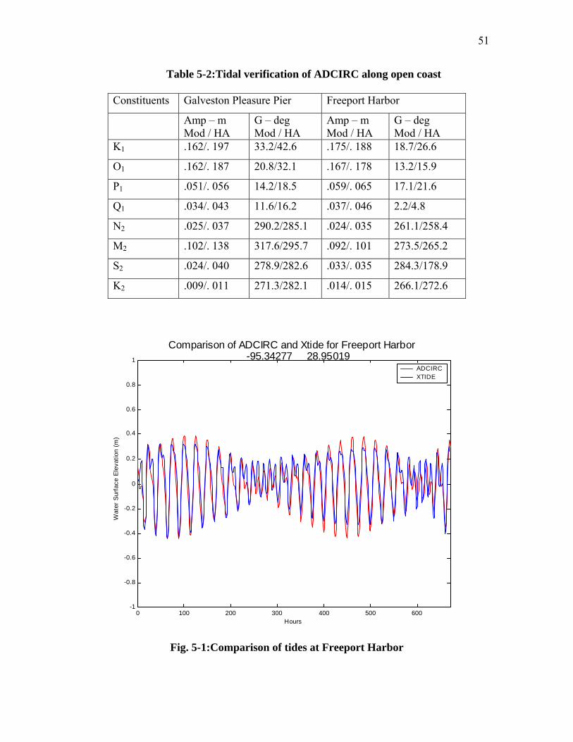
51

Table 5-2:Tidal verification of ADCIRC along open coast

Constituents Galveston Pleasure Pier Freeport Harbor

Amp – m Mod / HA

G – deg Mod / HA

Amp – m Mod / HA

G – deg Mod / HA

K1 .162/. 197 33.2/42.6 .175/. 188 18.7/26.6

O1 .162/. 187 20.8/32.1 .167/. 178 13.2/15.9

P1 .051/. 056 14.2/18.5 .059/. 065 17.1/21.6

Q1 .034/. 043 11.6/16.2 .037/. 046 2.2/4.8

N2 .025/. 037 290.2/285.1 .024/. 035 261.1/258.4

M2 .102/. 138 317.6/295.7 .092/. 101 273.5/265.2

S2 .024/. 040 278.9/282.6 .033/. 035 284.3/178.9

K2 .009/. 011 271.3/282.1 .014/. 015 266.1/272.6

0 100 200 300 400 500 600 -1

-0.8

-0.6

-0.4

-0.2

0

0.2

0.4

0.6

0.8

1

Hours

Wat

er S

urfa

ce E

leva

tion

(m)

Comparison of ADCIRC and Xtide for Freeport Harbor -95.34277 28.95019

ADCIRC XTIDE

Fig. 5-1:Comparison of tides at Freeport Harbor

52

0 100 200 300 400 500 600 -1

-0.8

-0.6

-0.4

-0.2

0

0.2

0.4

0.6

0.8

1

Hours

Wat

er S

urfa

ce E

leva

tion

(m)

Comparison of ADCIRC and XTIDE for Galveston Pleasure Pier -94.78747 29.28495

ADCIRC XTIDE

Fig. 5-2: Comparison of tides at Pleasure Pier

Comparison of tides was also made with NOS published time series. The

comparison is not as good as the tide gages record instantaneous water surface variations,

which includes wind waves. Fig. 5-3 shows this comparison and Fig. 5-4 shows the wind

speeds at the same location. It can be seen that differences are observed between

simulated and observed data whenever there is higher wind action in the region resulting

in wind waves. This is because the model ADCIRC in this particular case does not

account for wind.

53

0 100 200 300 400 500 -1

-0.8

-0.6

-0.4

-0.2

0

0.2

0.4

0.6

0.8

1

Hours

Wat

er S

urfa

ce E

leva

tion

(m)

Com parison of ADCIRC and NOS for GalvestonADCIRC TCOON

Fig. 5-3: Comparison of tides at Pleasure Pier with NOS gage

0 100 200 300 400 500 600 0

5

10

15

Hours

Win

d S

peed

(m/s

)

Wind Speed at Pleasure Pier

Fig. 5-4: Wind speeds at Pleasure Pier

54

It was only necessary to show that the model acceptably reproduced water levels

for all gauges to demonstrate approximate verification in a more global sense with

verification efforts concentrated on the study area. However, in order to demonstrate that

the overall verification was acceptable, all model to reconstructed prototype tidal time

series are presented in Appendix A. As shown, the comparisons are acceptable and

demonstrate that the ADCIRC model is properly reproducing tides throughout the general

area of interest as well as in the specific study area.

5.6 Tropical Storm Surge

The PBL model was used during this study and was coupled with ADCIRC in the

form of a wind file, which can be input to the ADCIRC model to simulate wind effects of

the storms of interest for the study area. Peripheral atmospheric pressures were assumed

equal to the standard atmospheric pressure of 1013 millibars (mb) and the geostrophic

wind speeds were specified as 6 knots in the same direction as the moving eye of the

storm. All additional data were computed from data contained in the National Oceanic

and Atmospheric Administration’s (NOAA) Hurricane DATabase (HURDAT) of tropical

storm events (Jarvinen, Neumann, and Davis 1988). This database is updated yearly and

now contains descriptions of all hurricane, tropical storm, and severe tropical depressions

that have impacted the east coast of the United States, Gulf of Mexico, and Caribbean

Sea from 1886 through 2002. The database contains latitude and longitude locations of

the eye of the hurricane with the corresponding central pressure and maximum wind

speeds at 6-hour intervals. The recent Hurricane Claudette (July 2003) was simulated by

using track data from weather databases, which contain track information: latitude,

longitude, time along with minimum pressure and maximum wind.

55

The goal of this component of the study was to compute frequency-of-occurrence

relationships for storm surge plus tide in the Freeport area. In order to develop these

relationships, it was necessary to identify tropical storms that have historically impacted

the study area. This was accomplished by making use of the tropical storm database

(Scheffner, et al, 1994) that was generated through simulation of 134 historically based

storm events along the east coast, Gulf of Mexico, and Caribbean Sea. The database uses

the HURDAT database described above as input. For 486 discrete locations along the

U.S. coast, peak storm surge values corresponding to storm events, which produced a

surge of at least 0.305 m, were archived and indexed according to event, location, and

surge magnitude. The database was used to select 26 storm events for the present study

beginning with the hurricane of 1886 and extending through Hurricane Claudette (2003).

These events, shown in Table 5-3, represent the selected historical set of storms. An

example plot of the storm track and location every 6 hours of Hurricane Claudette is

shown in Fig. 5-5. The track for each storm event of the historical training set is shown

in Appendix B.

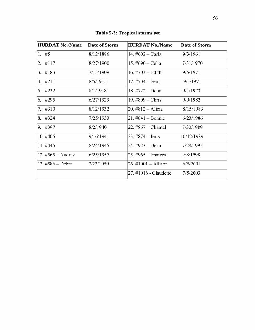
56

Table 5-3: Tropical storms set

HURDAT No./Name Date of Storm HURDAT No./Name Date of Storm

1. #5 8/12/1886 14. #602 – Carla 9/3/1961

2. #117 8/27/1900 15. #690 – Celia 7/31/1970

3. #183 7/13/1909 16. #703 – Edith 9/5/1971

4. #211 8/5/1915 17. #704 – Fern 9/3/1971

5. #232 8/1/1918 18. #722 – Delia 9/1/1973

6. #295 6/27/1929 19. #809 – Chris 9/9/1982

7. #310 8/12/1932 20. #812 – Alicia 8/15/1983

8. #324 7/25/1933 21. #841 – Bonnie 6/23/1986

9. #397 8/2/1940 22. #867 – Chantal 7/30/1989

10. #405 9/16/1941 23. #874 – Jerry 10/12/1989

11. #445 8/24/1945 24. #923 – Dean 7/28/1995

12. #565 – Audrey 6/25/1957 25. #965 – Frances 9/8/1998

13. #586 – Debra 7/23/1959 26. #1001 – Allison 6/5/2001

27. #1016 - Claudette 7/5/2003

57

-100 -99 -98 -97 -96 -95 -94 -93 -92 -91 -90 23

24

25

26

27

28

29

30

31

32

33

Freeport

Claudette, 09-15 JUL 2003

12-21

13-9

14-15

14-2115-3 15-9

15-15Latitude °

Longitude °

(a)

-96.2 -96 -95.8 -95.6 -95.4 -95.2

28.2

28.4

28.6

28.8

29

29.2

Freeport

Claudette, 09-15 JUL

15-15

Latitude °

Longitude °

(b)

Fig. 5-5: (a) Large and (b) small scale plots of Hurricane Claudette’s track

58

This set of tropical storms is verified by comparing National Ocean Survey (NOS)

measured tide gage records taken at Pleasure Pier and Freeport Harbor. These data are

ideal for storm event verification effort as it allows calibration of the radius of maximum

wind that is an important input to the PBL model to optimize the model for comparison

of the set of storms for the area of interest. Due to spin-up time of 10-15 days required for

tidal simulations, the decision was taken to compare storm surge elevations without tidal

forcing. Therefore, surge only time-series were constructed by removing the astronomical

tide from the raw NOS tide gage records, and the ADCIRC surge was computed without

tidal forcing. For example, Fig. 5-6 shows a time series of NOS data for Freeport for

Hurricane Claudette (2003). As is evident from Fig. 5-6, the storm surge is accurately

captured; however, the tides are not accurately simulated due to spin-up time required for

tidal simulation in the Gulf. In Fig. 5-7, surge-only data is shown, which is computed by

subtracting tides and pre-storm datum from the raw signal.

59

Claudette (7/9/2003)

-1

-0.5

0

0.5

1

1.5

2

0 1 2 3 4 5 6 7 8

Time, days from 7/9/2003

Surg

e - m

eter

sObserved Data Adcirc Freeport

Fig. 5-6: Raw surface elevation data for Hurricane Claudette at Freeport Harbor

60

Claudette (7/9/2003)

-0.5

0

0.5

1

1.5

2

0 1 2 3 4 5 6 7 8

T im e, days from 7/9/2003

Surg

e - m

eter

sO bserved Data Adcirc Freeport

Fig. 5-7: Surge only surface elevation data for Hurricane Claudette

NOS Data are available for Pleasure Pier for the period starting August 1957

through August 2003. Data for Freeport Harbor is available only for the period starting

March 1995 through August 2003. The data for Clear Lake is available starting August

1991. This period represents almost a 50-year period and encompasses majority of the

storms in the Galveston bay and Freeport.

All storms shown in Table 5-3 were simulated using ADCIRC model without

tide. Storm surge peak values for events before August 1957 were compared to anecdotal

data from National Hurricane Center’s historical archives by removing tides. Storm event

simulated hydrographs for events after August 1957 were compared to the NOS

hydrographs at Pleasure pier, Freeport Harbor and Clear Lake gage stations. Results and

61

comparisons of peak surge values in meters relative to mean sea level for each event for

which data are available are shown in Table 5-4.

Table 5-4: Comparison of storm surge computations with observed data measured

from MSL

Pleasure Pier

(m, msl)

Freeport Harbor

(m, msl)

Clear Lake shores

(m, msl)

Storm No.

ADCIRC NOS ADCIRC NOS ADCIRC NOS

1. #5 0.796 0.880 1.068

2. #117 2.141 0.788 1.216

3. #183 1.493 0.931 1.475

4. #211 3.059 1.372 3.369

5. #232 0.780 0.576 0

6. #295 1.875 0.917 1.123

7. #310 3.040 0.612 3.9232

8. #324 0.689 0.687 0.688

9. #397 0.264 0.270 0.37

10. #405 2.155 2.159 3.234

11. #445 1.002 1.351 2.391

12. #565 – Audrey 0.516 0.449 0.514

13. #586 – Debra 1.105 0.954 0.562 2.64

14. #602 – Carla 2.314 2.46 3.295 3.811

15. #690 – Celia 0.952 0.91 1.525 1.466

16. #703 – Edith 1.158 1.25 0.927 1.172

17. #704 – Fern 1.477 1.32 1.446 2.067

18. #722 – Delia 1.227 1.14 1.227 1.965

19. #809 – Chris 0.434 0.401 0.409 0.553

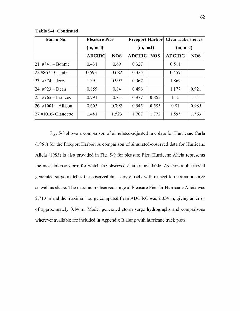
62

Table 5-4: Continued

Pleasure Pier

(m, msl)

Freeport Harbor

(m, msl)

Clear Lake shores

(m, msl)

Storm No.

ADCIRC NOS ADCIRC NOS ADCIRC NOS

21. #841 – Bonnie 0.431 0.69 0.327 0.511

22 #867 - Chantal 0.593 0.682 0.325 0.459

23. #874 – Jerry 1.39 0.997 0.967 1.869

24. #923 – Dean 0.859 0.84 0.498 1.177 0.921

25. #965 – Frances 0.791 0.84 0.877 0.865 1.15 1.31

26. #1001 – Allison 0.605 0.792 0.345 0.585 0.81 0.985

27.#1016- Claudette 1.481 1.523 1.707 1.772 1.595 1.563

Fig. 5-8 shows a comparison of simulated-adjusted raw data for Hurricane Carla

(1961) for the Freeport Harbor. A comparison of simulated-observed data for Hurricane

Alicia (1983) is also provided in Fig. 5-9 for pleasure Pier. Hurricane Alicia represents

the most intense storm for which the observed data are available. As shown, the model

generated surge matches the observed data very closely with respect to maximum surge

as well as shape. The maximum observed surge at Pleasure Pier for Hurricane Alicia was

2.710 m and the maximum surge computed from ADCIRC was 2.334 m, giving an error

of approximately 0.14 m. Model generated storm surge hydrographs and comparisons

wherever available are included in Appendix B along with hurricane track plots.

63

Carla (9/3/1961)

-0.5

0

0.5

1

1.5

2

2.5

0 2 4 6 8 10 12 14 16

Time, days from 9/3/1961

Surg

e - m

eter

sAdcirc Pleasure Pier Observed Data

Fig. 5-8: Simulated-observed data for Hurricane Carla (1961) for Pleasure Pier

Alicia (8/15/1983)

-0.5

0

0.5

1

1.5

2

2.5

3

0 1 2 3 4 5 6Tim e, days from 8/15/1983

Surg

e - m

eter

s

Observed Data Adcirc Pleasure Pier

Fig. 5-9: Simulated-observed data for Hurricane Alicia (1983) for Pleasure Pier

64

A spatial distribution snapshot plot of the maximum surge at the approximate

time of peak surge for Hurricane Claudette (2003) along the open coast area of Freeport

is shown in Fig. 5-10. Model results agree very well with observed data reported from

NOS database where storm surge of 1.3 - 2 meters above normal tides was observed and

both the barrier islands were inundated.

Model simulations for tidal elevations are considered to be acceptable for use in

the frequency analysis. Additionally, model results compare well to available storm surge

data for a variety of storm events and qualitatively compare well to post-storm visual

surveys. The conclusion of the tidal and storm surge verification effort is that the model

reasonably reproduces known historical events such as tide and tropical storms.

Water surface elevation (m)

2.05 1.65 1.25 0.85 0.45 0.05 -0.35 -0.75 -1.15

Fig. 5-10: Maximum surge at the approximate time of peak surge for Hurricane Claudette along the area of Freeport coast

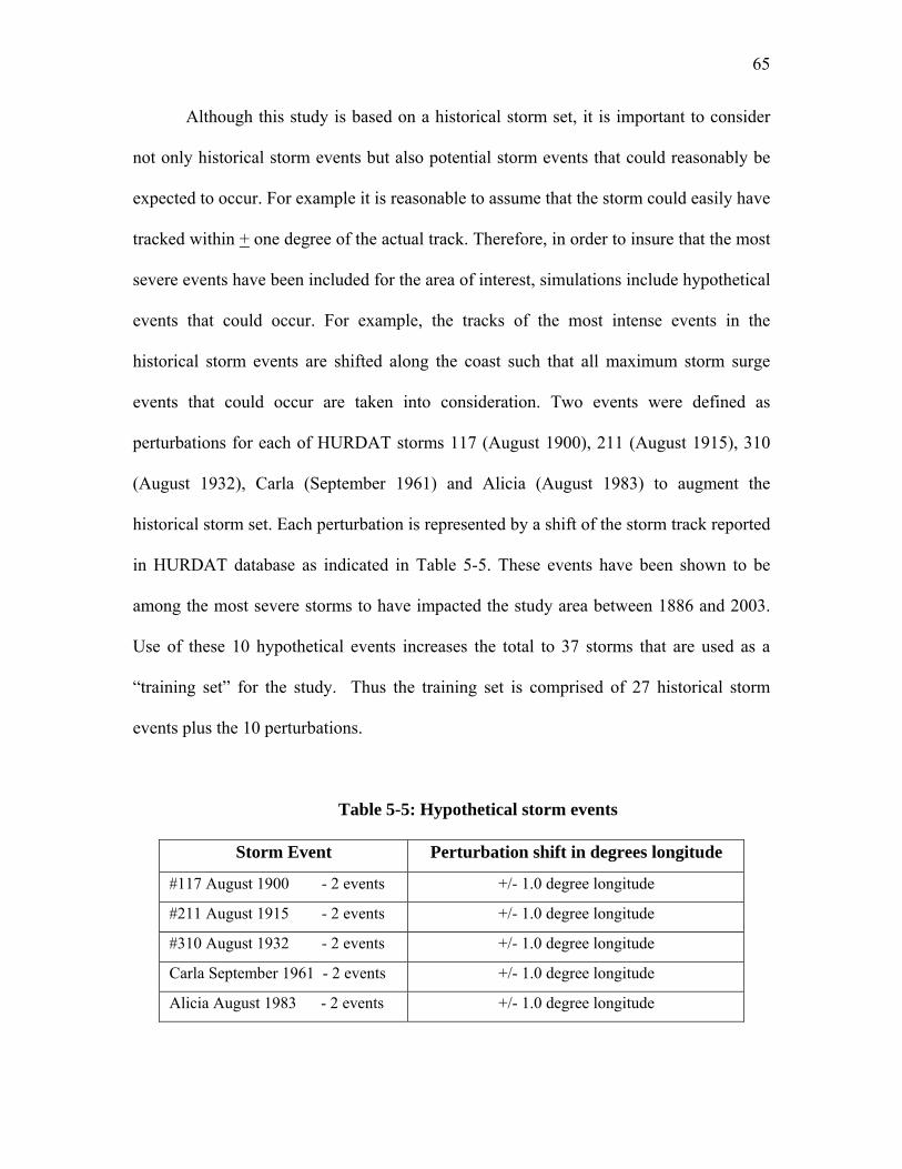
65

Although this study is based on a historical storm set, it is important to consider

not only historical storm events but also potential storm events that could reasonably be

expected to occur. For example it is reasonable to assume that the storm could easily have

tracked within + one degree of the actual track. Therefore, in order to insure that the most

severe events have been included for the area of interest, simulations include hypothetical

events that could occur. For example, the tracks of the most intense events in the

historical storm events are shifted along the coast such that all maximum storm surge

events that could occur are taken into consideration. Two events were defined as

perturbations for each of HURDAT storms 117 (August 1900), 211 (August 1915), 310

(August 1932), Carla (September 1961) and Alicia (August 1983) to augment the

historical storm set. Each perturbation is represented by a shift of the storm track reported

in HURDAT database as indicated in Table 5-5. These events have been shown to be

among the most severe storms to have impacted the study area between 1886 and 2003.

Use of these 10 hypothetical events increases the total to 37 storms that are used as a

“training set” for the study. Thus the training set is comprised of 27 historical storm

events plus the 10 perturbations.

Table 5-5: Hypothetical storm events

Storm Event Perturbation shift in degrees longitude

#117 August 1900 - 2 events +/- 1.0 degree longitude

#211 August 1915 - 2 events +/- 1.0 degree longitude

#310 August 1932 - 2 events +/- 1.0 degree longitude

Carla September 1961 - 2 events +/- 1.0 degree longitude

Alicia August 1983 - 2 events +/- 1.0 degree longitude

66

5.7 Application of EST

In order to establish the training set of storms 27 historical events and 10 storm

perturbations were used to produce a total of 37 events. Each of the 37 storms was

simulated without tide to produce a set of surge-only responses at the stations. The

storms are then assumed to have taken place at different phases of the astronomical tides:

1) high tide, 2) mean (MSL = 0.0) tide, and 3) low tide. It is further assumed that the

storm could occur during the lunar cycles of: 1) spring tide, 2) between spring and neap,

and 3) neap tide. Input vectors representing these phases of the tide are described above.

This combination of tide and lunar cycle produces 9 surface elevations for each of the 27

storm events of Table 5-3 and 10 hypothetical storm events at the station locations shown

in

Fig. 5-11. This procedure produces a total input/response vector training set of

333 (37*9), tide plus surge events for each station location. It is also considered that the

mid-tide level would have twice the probability of occurrence on the MHHW or the

MLLW. Similarly the mean tidal range would have twice the probability of occurrence as

spring or neap tide.

67

Fig. 5-11: Location of points used for input to EST model

The water surface elevation that is one of the response vectors for the EST

analysis was calculated as follows. Analysis of tidal values for the tides at Freeport

harbor show that the approximate peak tidal elevation at spring, mid, and neap cycle is

0.35, 0.268, and 0.20 m. The four primary model-generated diurnal and semi-diurnal

tidal constituents for the Freeport Harbor study area are the K1, O1, M2, and S2 with the

amplitudes of 0.137, 0.125, 0.07, and 0.02 m respectively. The values of spring and neap

tides are calculated using these constituents as follows assuming that most of the tidal

energy is contained in these constituents, using the relationship:

GULF OF MEXICO

BRAZOS RIVER

FREEPORT

68

spring high tide = K1 + O1 + M2 + S2

mid spring/neap high tide = K1 + O1

neap high tide = K1 - O1 + M2 + S2

This relationship generates an acceptable approximation of 0.352, 0.261, and

0.191 m versus 0.35, 0.268, and 0.2 m for the 9 combinations, as explained earlier, of

astronomical and lunar tidal effects. Therefore this relationship was used for all

locations. Similar steps are used for Galveston Pleasure Pier and Clear Lake locations.

The model simulations are used to generate a database of historical and

historically based storm events for use in generating maximum surface elevation

frequency-of-occurrence relationships at the sites as shown in Fig. 5-11. The statistical

approach used to generate multiple life-cycle simulations of storm-activity for the study

area and the subsequent post-processing of results to generate surge versus frequency-of-

occurrence relationships is described here.

An example set of 500 frequency relationships and the mean value for the

Freeport Harbor are shown in Fig. 5-12. Fig. 5-13 shows the mean value with the +/- one

standard deviation error bounds. The extreme event storm surge for locations around the

Freeport levee for 200, 100 and 50-year storms are shown in Fig. 5-14 through 5-16. The

storm surge frequency-of-occurrence tables for all the 35 locations are provided in

Appendix C.

Surge elevations are affected by many variables such as offshore bathymetry,

storm/shoreline orientation, location with respect to the Gulf of Mexico, and the local

topography. Therefore, the frequency-indexed surge distribution varies from one end of

the study area to the other.

69

0 1 2 3 4 5 6 7 8 9

10 11

10 20 30 40 50 60 70 80 90 100 110 120 130 140 150 160 170 180 190 200

Sur

face

Ele

vatio

n, m

Return Period ( )

Frequency Spread

Fig. 5-12: Frequency relationship for the Freeport Harbor for 500 simulations of 200 years

70

-1

0

1

2

3

4

5

6

7

1 0 2 0 3 0 4 0 5 0 6 0 7 0 8 0 9 0 1 0 0 1 1 0 1 2 0 1 3 0 1 4 0 1 5 0 1 6 0 1 7 0 1 8 0 1 9 0 2 0 0

Surfa

ce E

leva

tion,

m

R e tu rn P e rio d (ye a rs )

F re q u e n c y C u rve

8 0 % C o n fid e n c e + /- 1 S .D .M e a n

Fig. 5-13: Mean Value of surface elevation with standard deviation bounds for Freeport Harbor

71

Values are in meters

Fig. 5-14: 200 year storm surge values around the Freeport Levee System

Values are in meters

Fig. 5-15: 100 year storm surge values around the Freeport Levee System

72

Values are in meters

Fig. 5-16: 50-year storm surge values around the Freeport Levee System

The ADCIRC-EST approach can thus be used to estimate and predict life cycle storm

surge values at any given site as shown above. These values can hence be used for design

purposes or for evacuation and planning purposes. The model SLOSH is currently used

by federal authorities in the United States for hurricane evacuation and planning. The

next section presents a comparison between this approach and the SLOSH approach.

73

6 COMPARISON WITH SLOSH

The SLOSH numerical model is used to prepare an atlas of pre-computed surges.

On-site computations with several tracks, tropical cyclone intensities and sizes may

require many computer runs. During a real time situation this can overload computer

facilities and personnel, and require unacceptably time consuming analysis of the output.

To generate a database of pre-computed atlases of storm surges for a particular

basin with inland water bodies and complicated terrain features, recourse is made to a

tropical cyclone climatology, which gives a broad view of the tropical cyclone types

likely to affect a given region. Historical tropical cyclones affecting a region are stratified

into preferred track directions, intensities, and sizes. Such families of equally spaced,

parallel tracks for surge computations gently curve to reflect climatological data, but

should all correspond in the vicinity of the landfall points.

6.1 Methodology of Storm Atlas

The family of tracks account for alternate landfall points for a given direction

along a coastal area of interest (or else alternate distances from the coast for alongshore

moving tropical cyclones). It is recognized that the generated surge normally is strongly

dependent on the angle the track makes with the coast, several hours before and after

landfall. Thus, the remaining track segments affect the surge only mildly. Thus, although

the location of a tropical cyclone far out to sea and its landfall point may be significantly

in error, the family, or families, representing the broad approach to land can be used to

estimate the likely surge consequences.

For simplification, it is assumed that the cyclone translation speed, central

pressure and size remain constant along the track. Alternate values of these parameters

74

can be used for each track family to provide a more comprehensive database. The

embedded, identical tropical cyclone model in each family of tracks also can be designed

to alter the tropical-cyclone central pressure and size with time after landfall to represent

any explosive filling and core changes of the tropical cyclone.

After a study of potential surges with idealized tracks from the atlas, runs are then

made to fine tune a surge forecast that includes relevant details from the actual cyclone.

6.2 Maximum Envelope of Waters (MEOW)

An atlas of pre-computed surges can be a bulky document and collating the

several possible tropical cyclone conditions from the many into a composite potential of

surges is a demanding chore. Since each computer run gives an envelope of highest

waters in a basin for the life history of a tropical cyclone, it is a simple computer chore to

determine the highest possible surge at all vulnerable coastal locations from a particular

family of tracks. The resulting map is called a Maximum Envelope of Waters, or MEOW.

Model runs are made using hypothetical tropical cyclones stratified by the

Saffir/Simpson scale of intensity categories and sizes. To generate the MEOW, the

maximum surge value from the entire family of cyclones at each grid square of a basin is

saved; regardless of which cyclone was responsible. The resulting composite of peak

surges makes up a MEOW such as that shown in Fig. 6-1. Other MEOWs can be

developed for a range of cyclone profiles and conditions. This provides an easily

accessible summary of the "worst case" surge scenario given the uncertainty in the

current forecast situation.

75

6.3 Storm Atlas for Harris/ Brazoria County

The model SLOSH was run for imaginary storms with varying intensities

(category 1–5) and the effect of storm making landfall at a relative distance from

Galveston channel was studied. These results were produced in the form of Maximum

Storm Surge Penetration Maps in the Storm Atlas (College of Architecture 1994).

There are five MEOWs, which indicate the worst case MEOWs (or MOMS,

Maximum of MEOWs) for each category of hurricane making landfall from 87 nautical

miles right to 70 nautical miles left of Galveston channel. For each of these landfall areas,

a high and a low MEOW were produced.

The high (maximum) is produced by taking all of the various MEOW movement

directions and forward movement speeds and using the high surge elevations. The low

(minimum) is produced by using the lowest surge elevations. As will be noticed, the

differences between high (maximum) and low (minimum) surge estimates for the same

category of hurricane are quite extreme. This illustrates the extreme range of possibilities

in modeling with SLOSH as only hypothetical events are used.

76

Fig. 6-1: MEOW for Hurricane Carla (1961) for Galveston Bay (units of elevation are in feet (Jelesnianski et al, 1992))

77

6.4 Comparison with ADCIRC

For comparison of ADCIRC simulated storm surge with SLOSH predicted surges,

the hurricanes used in the study were arranged according to the approach used in the

storm atlas that is on the basis of the Saffir-Simpson scale category and the distance from

Galveston ship channel as shown in Table 6-1.

Table 6-1: Characteristics of hurricane database used in the study

Storm No. Pressure (mb)

Distance from Galveston channel

(n-miles)

Max Wind (knots) Category Radius Max

Wind (nm)

5 984 131.698 85 2 21.28

117 964 17.921 115 4 41.37

117(+1.0) 964 56.765 115 4 41.37

117(-1.0) 964 42.596 115 4 50.83

183 986 43.156 120 4 31.91

211 953 35.912 125 4 50.83

211(+1.0) 953 86.889 125 4 17.73

211(-1.0) 953 14.758 125 4 50.83

232 980 115.608 90 2 50.83

295 988 56.221 75 1 40.19

310 955 19.599 125 4 31.91

310(+1.0) 942 80.955 125 4 41.37

310(-1.0) 942 40.514 125 4 41.37

324 981 352.513 80 1 44.92

397 973 106.709 70 1 34.28

405 977 86.896 80 1 50.83

78

Table 6-1: Continued

Storm No. Pressure (mb)

Distance from Galveston channel

(n-miles)

Max Wind (knots) Category Radius Max

Wind (nm)

445 987 126.904 120 4 50.83

565 – Audrey 972 88.699 125 4 50.83

586 – Debra 989 34.993 75 1 50.83

602 – Carla 931 171.81 145 5 49.82

602 – Carla(+1.0) 931 246.148 145 5 49.82

602 – Carla(-1.0) 931 97.423 145 5 49.82

690 – Celia 950 232.38 110 3 29.55

703 – Edith 978 249.656 140 5 28.37

704 – Fern 979 139.846 80 1 43.73

722 – Delia 987 56.211 60 1 50.83

809 – Chris 994 77.112 55 1 37.82

812 – Alicia 963 38.474 100 3 22.46

812 – Alicia(+1.0) 963 107.395 100 3 22.46

812 – Alicia(-1.0) 963 7.211 100 3 37.82

841 – Bonnie 992 53.89 75 1 18.91

867 – Chantal 984 34.603 70 1 26

874 – Jerry 983 26.869 65 1 20.09

923 – Dean 999 42.472 40 1 50.83

965 – Frances 990 195.874 55 1 50.83

1001 – Allison 1003 40.109 45 1 50.83

1016 - Claudette 983 127.365 75 1 41.37

MEOW charts from the storm atlas are read and the corresponding maximum and

minimum values for a storm are read based on its distance from the Galveston ship

channel and its category. These values are then plotted along with ADCIRC simulated

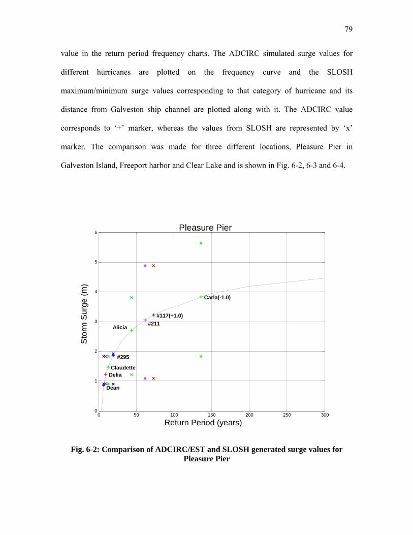
79

value in the return period frequency charts. The ADCIRC simulated surge values for

different hurricanes are plotted on the frequency curve and the SLOSH

maximum/minimum surge values corresponding to that category of hurricane and its

distance from Galveston ship channel are plotted along with it. The ADCIRC value

corresponds to ‘+’ marker, whereas the values from SLOSH are represented by ‘x’

marker. The comparison was made for three different locations, Pleasure Pier in

Galveston Island, Freeport harbor and Clear Lake and is shown in Fig. 6-2, 6-3 and 6-4.

0 50 100 150 200 250 300 0

1

2

3

4

5

6 Pleasure Pier

#211

Return Period (years)

Sto

rm S

urge

(m)

Alicia

#117(+1.0)

Claudette Delia

Dean

Carla(-1.0)

#295

Fig. 6-2: Comparison of ADCIRC/EST and SLOSH generated surge values for Pleasure Pier

80

0 50 100 150 200 250 300 0

1

2

3

4

5

6

#211(+1.0)

Return Period (years)

Sto

rm S

urge

(m)

Freeport Harbor

#310(+1.0)

Claudette

#211 Alicia

Debra

Carla(-1.0)

Fig. 6-3: Comparison of ADCIRC/EST and SLOSH generated surge values for Freeport Harbor

81

0 50 100 150 200 250 300 0

1

2

3

4

5

6

7

8

Return period (years)

Sto

rm S

urge

(m)

Clear Lake

#310(+1.0)

Alicia

#211

Debra

Dean

Claudette

Carla(-1.0)

Fig. 6-4: Comparison of ADCIRC/EST and SLOSH generated surge values for Clear Lake

As evident from the Figs, there is a large amount of scatter in the case of SLOSH

values, especially in the case for Freeport harbor. This may be because the SLOSH runs

with simulated hurricanes whose distances were measured from Galveston ship channel.

The distance between Freeport Harbor and the ship channel being 80 miles, the SLOSH

analysis is not accurate for Freeport area. In the case of storm surge at Freeport due to

Hurricane Alicia (1983), SLOSH estimates that a hurricane of its intensity and at a

distance of 38.45 n-miles from Galveston ship channel should produce a maximum surge

of 3.96 m and a minimum surge of 1.2192 m. However, the ADCIRC generated surge

due to Alicia was 1.023 m. The anecdotal surge due to Alicia (Garcia and Flor, 1984) was

reported to be around 1 m. Thus SLOSH over-estimates the surge in this case. This is due

82

to the fact that Alicia made landfall around 50 miles to the right of Freeport looking

landward. In the northern hemisphere due to rotation of earth, the effect of storm surge is

more pronounced on the right side of hurricane center rather than left side. This effect is

not taken into account in the approach used for producing the storm atlas using SLOSH.

Hence the storm surge values from the storm atlas are accurate only for centrally located

regions in the SLOSH grid. Also this approach assumes that all the storms of same

category making landfall within the distance of 46 n-miles right to 23 n-miles left of a

location will produce the same surge. This may be true for some ideal cases but imagine

an intense hurricane of category 5 having Rmax (Radius of maximum winds) of 29 n-

miles making landfall 10 miles right of the central location. In this case areas 35-52 n-

miles from the central location will experience high values of surge of the order of 3-4

meters but the areas on the left hand side of landfall location will experience much less

storm surge, assuming the bathymetry around the area is similar.

Some of the problems associated with SLOSH are thus identified as follows:

1. Although storm-induced flooding along the coast of the United States can be

predicted fairly accurately using SLOSH, storm surges in bays and estuaries are often

poorly predicted using this method because of irregular coastline and local topography.

2. The simplification used for preparing of these atlases is that the cyclone

translation speed, central pressure and size remain constant along the track. This

assumption is generally not true. For example the hurricane of 1915 (7/13/1915) had its

maximum winds (120 knots) at a distance of approximately 120 miles from its landfall

and had winds of much lower value (85 knots) at landfall. Thus the assumption of

constant size of storm and constant winds results in over-estimation of surges.

83

3. For the same landfall location and category storms, the storm atlas gives the

same results. It is accepted that the peak surge on the open coast is not always

monotonically related to the parameter, maximum wind speed of the storm. In fact, the

peak surge may increase or decrease according to the manner in which the other storm

parameters are affected by the change in maximum wind speed. The pressure drop, size

scale and shape of the wind profile also have an effect on the peak surge. For example

Hurricane Camille (1969) that was an ordinarily sized storm though it was a category

five storm and resulted in storm surge of 6 meters in Gulfport, Mississippi. However,

SLOSH gives prominence to maximum wind speeds during analysis.

4. The SLOSH model’s polar grid as shown in Fig. 3-2 is generally very coarse

compared to the ADCIRC grid. For the study area Freeport, a high-resolution grid was

needed to effectively calculate storm surges all along the existing levee system. The

SLOSH grid covers the whole Freeport area in just 24 squares.

5. Since we do not completely understand the processes of hurricane formation

and hence cannot model these accurately, using empirical relations to simulate them is

a wrong approach. Thus the approach of using historical storms to generate database of

storm surge and then using a return period concept to calculate maximum storm surges

may be more reliable instead of just simulating different storms, where not all the

storms have similar features. Using the same coefficients for all these different storms

also is not advisable.

6. Risk assessment by definition necessitates a probabilistic approach whereas

SLOSH uses an event-driven approach.

The SLOSH model results are taken manually from the contour plots provided in

the Storm Atlas. Due to difficulties reading the SLOSH values from the contour plots, the

84

values in the table should only be considered approximate (+/- 0.5 feet) and only used for

a broad and general comparison.

6.5 Alternate Approach

The database consisting of 37 storms, which is extended to 333 storms with

addition of neap, spring tides, high and low tides, is used for this EST analysis. Two

different type of analysis were done. In one case the pressure difference between the eye

of the hurricane and ambient is used as a response vector with all other input vectors

remaining the same as in storm surge analysis with addition of storm surge associated

with that hurricane as an input vector. The other case is repeated with maximum wind

speed being used as a response vector. The lower bands of pressure difference values and

maximum wind speeds for different categories of hurricanes, based on Saffir Simpson

scale are read from Table 6-2. These two plots are shown in Fig. 6-5 and Fig. 6-6.

Table 6-2: Saffir Simpson scale

Category Pressure Difference (mb) Maximum Wind Speed (knots)

1 33 64

2 33 83

3 48 96

4 68 114

5 93 135

85

-20

0

20

40

60

80

100

120

140

160

180

200

10 20 30 40 50 60 70 80 90 100 110 120 130 140 150 160 170 180 190 200

Max

imum

Win

d Sp

eed

(kno

ts)

Return Period (years)

+/- 1 S.D.

Mean

Fig. 6-5: Frequency plot for maximum wind speeds

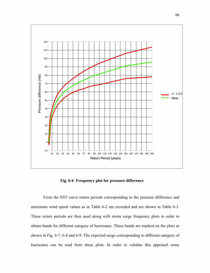
86

-10

0

10

20

30

40

50

60

70

80

90

100

110

120

10 20 30 40 50 60 70 80 90 100 110 120 130 140 150 160 170 180 190 200

Pre

ssur

e di

ffere

nce

(mb)

Return Period (years)

+/- 1 S.DMean

Fig. 6-6: Frequency plot for pressure difference

From the EST curve return periods corresponding to the pressure difference and

maximum wind speed values as in Table 6-2 are recorded and are shown in Table 6-3.

These return periods are then used along with storm surge frequency plots in order to

obtain bands for different category of hurricanes. These bands are marked on the plots as

shown in Fig. 6-7, 6-8 and 6-9. The expected surge corresponding to different category of

hurricanes can be read from these plots. In order to validate this approach some

87

hurricanes were simulated and checked for their acceptability with the return periods

predicted.

Table 6-3: Return periods for different categories of hurricanes

Category Return Periods based on

Pressure Difference, years

Return Periods based on

Wind speed, years

1 - -

2 12 32

3 26 45

4 52 62

5 168 116

6.6 Validation

In order to validate this approach some more hypothetical hurricanes were

simulated in addition to the existing ones. Since SLOSH model assumes that the size and

intensity of a hurricane remain constant throughout its track, Hurricane Carla (1961) was

manipulated to obtain medium range category 2,3,4 and 5 hurricanes. Further, the track

of Carla was perturbed by shifting it by -1.0 and –1.5 degree longitude from its normal

track to obtain the maximum effect around the Freeport and Galveston Bay areas

respectively. The storm surges from these hurricanes were plotted on the categorized

storm surge return period graphs and are shown in Figures 6-7, 6-8 and 6-9.

88

0 50 100 150 200 250 3000

1

2

3

4

5

6 Pleasure Pier

#211

Carla(-1.5) Cat 4 Carla(-1.5) Cat 5

Carla(-1.5) Cat 3

Carla(-1.5) Cat 2

Return Period (years)

Sto

rm S

urge

(m)

Alicia

#117(+1.0)

Claudette Delia

Dean

5 4 3 2 1

Fig. 6-7: Category bands for Galveston Pleasure Pier

89

0 50 100 150 200 250 3000

1

2

3

4

5

6

#211(+1.0)

Carla(-1.5) Cat 4

Carla(-1.5) Cat 5

Carla(-1.5) Cat 3

Carla(-1.5) Cat 2

Return Period (years)

Sto

rm S

urge

(m)

Freeport Harbor

#310(+1.0)

Claudette

#211 Alicia

Debra

1 2 3 4 5

Fig. 6-8: Category bands for Freeport Harbor

90

0 50 100 150 200 250 3000

1

2

3

4

5

6

7

8

Carla(-1.5) Cat 4

Carla(-1.5) Cat 5

Carla(-1.5) Cat 3

Carla(-1.5) Cat 2

Return period (years)

Sto

rm S

urge

(m)

Clear Lake

#310(+1.0)

Alicia

#211

Debra

Dean

Claudette

1 2 3 4 5

Fig. 6-9: Category bands for Clear Lake

91

The return periods for pressure difference are used in this study, as they seem

to be more accurate and also conform to the HURISK return periods (Neumann C.J.

1994). The reason for this may be because maximum wind speeds are a function of

central pressure difference and radius of maximum winds (Jelesnianski 1972), and since

we still can not simulate Radius of maximum winds accurately, there seems to be some

flaw in using maximum winds for calculating return periods for categories of hurricanes.

Also, the fact that hurricane database consists of wind speeds greater than 64 knots,

introduces some error in EST analyses for lower values of wind speeds response vector.

The hypothetical hurricanes like Carla (-1.0) and (-1.5) longitude whose

maximum effect occurs at the respective locations Freeport and Galveston Bay fall well

within the bands for their category as predicted. This is because these hurricanes make

landfall within the distance of 30-50 miles left of the respective sites. Hence these

hurricanes produce their maximum surge at these locations. As we move away from the

landfall location, surge will reduce. However on the right hand side of the landfall

location due to opposing wind directions surge is also reduced.

Let us consider the case of Hurricane #211. It was a medium range category 4

hurricane according to the Saffir Simpson scale. It made landfall at a distance of 31.2

miles from Galveston ship channel. It produced a surge consistent with the expected

value read from Fig. 6-7 for Pleasure Pier. However it has a different impact at Freeport.

It made landfall at a distance of 18 miles to the right and resulted in a surge of 1.34

meters. This is much less than its expected value that is within range of 2.6-4.5 meters.

This is due to its making landfall right of Freeport. Thus it had an effect of a category 2

hurricane in the vicinity of Freeport.

92

Similarly Hurricane Alicia made landfall 33.5 miles left of ship channel and

resulted in a storm surge of 2.7 meters and lies within its expected category in the

frequency curves. However with respect to Freeport, it made landfall right of Freeport at

a distance of 15 miles. Here again the frequency plots do not capture the storm surge

associated due to it. This is again due to its making landfall right of Freeport.

The return period bands cover a wide range of storm surge, thus in order to

predict a value that a hurricane can result, care must be taken. Storm surge being a

complicated process, dependent on a large number of parameters, the predicted value will

always have some inherent errors in it. Since the EST approach tries to take into effect all

the factors that influence storm surge, the approach is more reliable compared to other

approaches. A hurricane belonging to a category can, still be classified further into

weaker, modest and stronger based on the ranges. Hence a weaker hurricane would

correspond to a lower value of storm surge in that band and so on. The effect of distance

of the site from landfall also plays an important role in the storm surge expected at that

site. Based on the radius of maximum winds for the hurricane, the value must be selected

from the plots considering the fact that surge is greater at a distance of around 30-40

miles from the landfall location. As we move away from the landfall location the storm

surge is greatly reduced. Thus relative distance plays a very important role in storm surge

expected due to a hurricane.

The present prediction and forecasting techniques do not accurately capture the

effect of relative distance. Thus a method needs to be established in order to quantify

storm surge due to a hurricane of given intensity and size on the basis of its relative

distance from the landfall location. The prevalent forecasting techniques do a good job in

93

estimating maximum surge that can be expected based on Saffir-Simpson scale

category of storms.

94

7 CONCLUSIONS

The results of this thesis illustrate the use of the hydrodynamic model ADCIRC in

conjunction with statistical model EST for storm surge simulation and generation of

frequency return curves for a location. Comparisons have been presented that show

model output from ADCIRC and observed water level data for various hurricanes that

have significantly impacted Texas coast during last 117 years.

The simulated data for most of the hurricanes compares well with the measured

data wherever available. The model was able to accurately simulate the time and duration

of the highest storm surge level. However the model is not able to fully capture storm

surges due to tropical storms like Allison (2001). This inadequacy most likely results

from the simplified vortex flow representation of the wind field by the wind model PBL,

which may not accurately model the actual hurricane wind field particularly for a tropical

storm as a storm approaches and passes over a coastal boundary. The other cause may be

the method used to estimate the radius of maximum winds, which is the nomograph of

Fig. 2-1. Though this nomograph in general is able to predict the radius of maximum

winds, it is not able to do so for all storms equally as well. In this study the observed

values of radius were used wherever available as in Hurricane Claudette (2003) resulting

in fairly accurate storm surge simulation as shown in Fig. 5-7. Another factor may be that

the modeled distribution of wind magnitudes along the axis of storm may not be

representative of the actual storm, where wind speeds may not decay at the rate assumed

by the PBL model. The approach used in this study of using the whole Gulf of Mexico as

the computation domain takes care of the limitations of PBL model near to the shore.

The study extends the storm surge simulation using the EST model to arrive at

life-cycle return period curves for storm surge at a particular location. These values can

95

be used to give a realistic idea of typical ”design” storm surge values that may help

engineers to design new structures and maintain existing structures. EST encompasses all

the parameters that affect the storm surge at a location for an individual hurricane like

relative distance from landfall. Thus the results give a more realistic picture of the

damage potential to the engineers.

This approach is also compared with the SLOSH approach used by federal

authorities to delineate coastal areas susceptible to hurricane storm surge flooding and

evacuation studies. The shortcomings in the model SLOSH and the storm atlas approach

are pointed out in the study. An alternate way for estimating storm surge at a location

based on Saffir-Simpson categorization scale of hurricanes is presented in the study. This

method utilizes the database of historical and hypothetical storms to arrive at return

periods for different categories of hurricane and then uses these periods for estimating

storm surges due to different category of hurricanes.

This approach needs to be applied for localized areas, as there are many local

factors that may influence the storm surge. The local bathymetry may play an important

role in the final storm surge value; hence the computational grid used for populating the

database should have required resolution in order to capture the local bathymetry. The

shape of the coastline also has a strong effect on the size of a storm surge. A concave

coastline is favored for greater storm surge, as water can be funneled toward the center of

the coastline. For example, the coast of North Carolina has many concave areas that can

influence the size of a storm surge. For example, in 1996, Hurricane Fran made landfall

at Cape Fear, NC and produced a storm surge of 3.2 m at Carolina Beach, NC. Hurricane

Hazel (1954) made landfall at the border of North and South Carolina, as a rapidly

moving hurricane. This area of North Carolina's coastline to the right of Hazel was

96

concave. Hazel was also a stronger, faster moving storm than Fran and it produced a

peak storm surge of 5.5 m on the south facing beaches south west of Carolina Beach,

while Carolina Beach had a peak storm surge of less than 3.0 m. Hence these coastline

effects again call for a good resolution of the computational grid.

There are certain improvements that can be made to the model. One is to include

shoaling effect. This refers to water forced from deep water into shallow water, where it

converges to the shoreline. The more shoaling that occurs, the higher the potential storm

surge. The waves also play an important role in potential storm surge. Strong hurricane

winds may result in high wave setups. Hence coupling of the hydrodynamic ADCIRC

model with a wave model would be helpful in estimating these factors. Also, high rainfall

amounts can lead to fresh water flooding, which can exacerbate the storm surge problem.

If a hurricane makes landfall in a location where several rivers empty into the ocean, the

runoff from the rivers can increase flooding. An example of this is Bangladesh, which is

located in a low-lying flood plain where several rivers empty into the Indian Ocean.

Future models may also include the effect of rainfall and river-runoffs to completely

calculate and estimate storm surges.

After evaluating the limitations of the present storm surge calculation and

estimation approach, it still provides useful information about surge levels for sites,

particularly for sites that are located to the east of a storm. The good feature of this

approach is its relative simplicity, as it can model a storm using only the most basic

information. Also as it is based on actual historical storm rather than possible

hypothetical ones, it is more credible.

97

REFERENCES

Bodine, B.R., (1971) “Storm surge on the open coast: fundamentals and simplified

prediction.” Corps of Engineers Technical Memorandum No. 35, USACE, WES,

Vicksburg, MS.

Borgman, L.E., Miller, M.C., Butler, H.L., and Reinhard, R.D., (1992) Empirical

simulation of future hurricane storm histories as a tool in engineering and Economic

Analysis. Proc. Civil Engineering in the Oceans, ASCE, New York, 2-5.

Borgman, L.E. and Scheffner, N.W., (1991) “The simulation of time sequences of wave

height, period, and direction.” TR-DRP-91-2. US Army Corps of Engineers, Waterways

Experiment Station, Vicksburg, MS.

Cardone, V.J., Greenwood, C.V., and Greenwood, J.A., (1992) “Unified program for the

specification of hurricane boundary layer winds over surfaces of specified roughness,”

contract report CERC-92-1, US Army Corps of Engineers, Waterways Experiment

Station, Vicksburg, MS.

Chow, S (1971) “A diagnostic model of the hurricane PBL.” Journal of Atmospheric

Sciences 29(2), 419–426.

College of Architecture, (1994) ”Storm atlas for Brazoria, Galveston and Harris

Counties.” Texas A&M University, College Station, TX.

Flather, R.A., (1988) “A numerical model investigation of tides and diurnal-period

continental shelf waves along Vancouver Island.” Journal of Physical Oceanography 18,

115-139.

Garcia, A. W. and Flor, T. H., (1984) “Hurricane Alicia storm surge and wave data,”

Technical report CERC-84-6, US Army Corps of Engineers, Waterways Experiment

Station, Vicksburg, MS.

Ho, F.P., (1987) “Hurricane climatology for the Atlantic and Gulf coasts of the United

States.” NOAA Technical Report NWS 38, NOAA, Washington, DC.

Jarvinen, B.R., Neumann, C.J., and Davis, M.A.S., (1988) “A tropical cyclone data tape

for the North Atlantic Basin, 1886-1983: Contents, limitation and uses,” NOAA Technical

Memorandum NWS NHC 22, NOAA, Washington, DC.

98

Jelesnianski, C.P., (1972) “SPLASH (Special program to list amplitudes of surges

from hurricanes)” NOAA Technical Memorandum NWS TDL-46, NOAA, Washington,

DC.

Jelesnianski, C.P., (1967) “Numerical computation of storm surges with bottom stress.”

Monthly Weather Review, 95,740-756.

Jelesnianski, C.P., Chen J. and Shaffer W.A., (1992) “SLOSH: Sea, lake, and overland

surges from hurricanes.” NOAA Technical Report NWS 48, NOAA, Washington, DC.

Jelesnianski, C.P. and Taylor, A.D., (1973) “A preliminary view of storm surges before

and after storm modifications.” NOAA Technical Memorandum ERL WMPO-3, Weather

Modification Program Office, Boulder CO.

Kolar, R.L., Gray, W.G., Westerink, J.J., and Luettich, R.A. (1994) “Shallow water

modeling in spherical coordinates: Equation formulation, numerical implementation, and

application,” Journal of Hydraulic Research 32(1), 3-24.

Le Provost, C., Genco M. L., Lyard F., Vincent P., and Canceil P. (1994) “Spectroscopy

of the world ocean tides from a finite element hydrodynamic model,” Journal of

Geophysics Research 94, 777-797.

Luettich, R.A., Westerink, J.J., and Scheffner, N.W., (1992) “ADCIRC: An advanced

three-dimensional circulation model for shelves, coasts, and estuaries Report 1:Theory

and methodology of ADCIRC-2DDI and ADCIRC-3DL,” Technical report DRP-92-6,

US Army Engineer Waterways Experiment Station, Vicksburg, MS.

Neumann C.J., (1994) “ The National Hurricane Center Risk Analysis Program

(HURISK),” Science Applications International Corporation, Miami, FL.

Platzman, G.W., (1963) “The dynamical prediction of wind tides on Lake Erie.”

Meteorological Monographs, 4, 44-48.

Scheffner, N.W., Carson, F.C., Rhee, J.P., Mark, D.J., (2003) “Coastal erosion study for

the open coast from Sabine Pass to San Luis Pass, Texas: Tropical storm surge frequency

analysis,” US Army Corps of Engineers, Waterways Experiment Station, Vicksburg, MS.

Scheffner, N. W., Clausner, J. E., Militello, A., Borgman, L. E., Edge, B. L., and Grace,

P. E, (1999) “Use and application of the empirical simulation technique: Users guide,”

99

Technical Report CHL-99-21, US Army Corps of Engineers, Waterways Experiment

Station, Vicksburg, MS.

Scheffner, N.W., Mark D.J., Blain, C.A., Westerink, J.J., and Luettich, R.A., (1994)

“ADCIRC: An advanced three-dimensional circulation model for shelves, coasts, and

estuaries report 5:A tropical storm data base for the East and Gulf of Mexico coasts of the

United States,” Technical Report DRP-94-4, U.S. Army Corps of Engineers, Waterways

Experiment Station, Vicksburg, MS.

Wanstrath, J.J. Reid, R.O., (1976) “Storm surge simulation in transformed coordinates”,

Technical Report No. 76-3, US Army Corps of Engineers, Waterways Experiment

Station, Vicksburg, MS.

Westerink, J.J., Luettich, R.A., and Scheffner, N.W., (1993) “ADCIRC: An advanced

three-dimensional circulation model for shelves, coasts, and estuaries report 3:

Development of a tidal constituent database for the western North Atlantic and Gulf of

Mexico,” Technical Report DRP-93-2, US Army Corps of Engineers, Waterways

Experiment Station, Vicksburg, MS.

100

APPENDIX A

COMPARISON OF MODEL GENERATED TIDES AND XTIDE

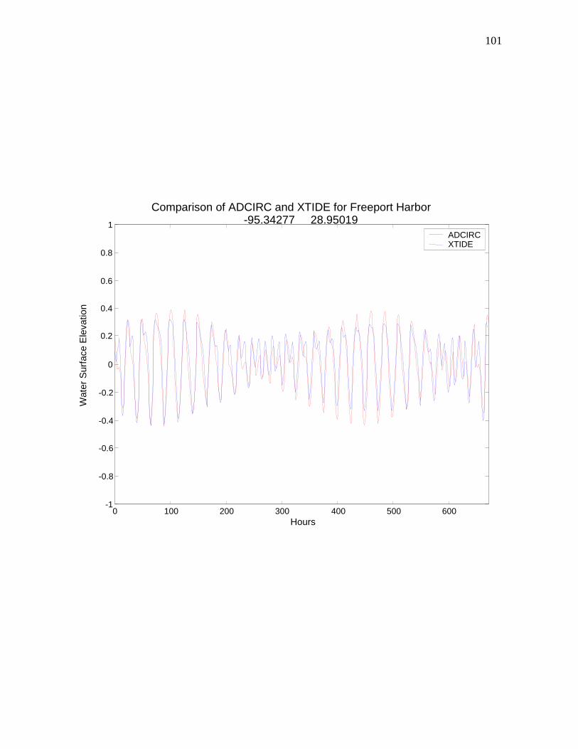
101

0 100 200 300 400 500 600 -1

-0.8

-0.6

-0.4

-0.2

0

0.2

0.4

0.6

0.8

1

Hours

Wat

er S

urfa

ce E

leva

tion

Comparison of ADCIRC and XTIDE for Freeport Harbor -95.34277 28.95019

ADCIRCXTIDE

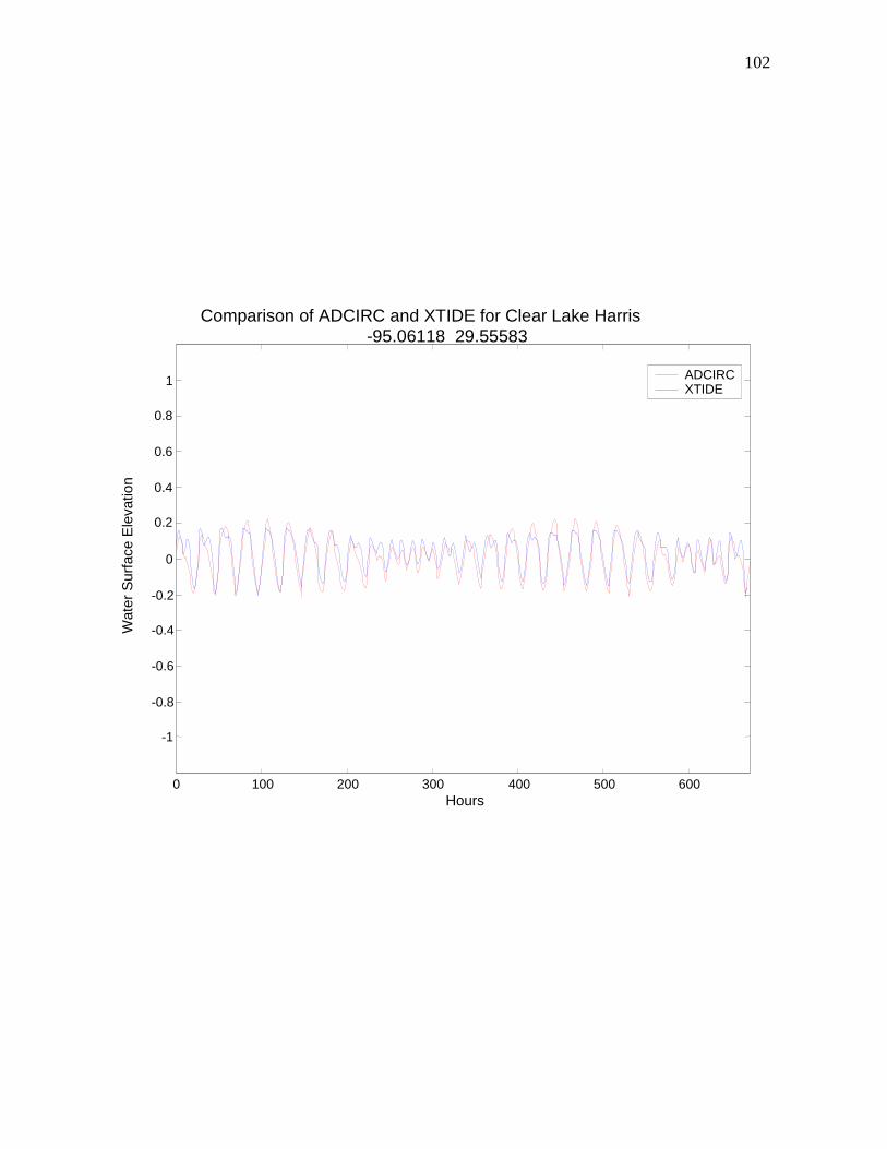
102

0 100 200 300 400 500 600

-1

-0.8

-0.6

-0.4

-0.2

0

0.2

0.4

0.6

0.8

1

Hours

Wat

er S

urfa

ce E

leva

tion

Comparison of ADCIRC and XTIDE for Clear Lake Harris P k -95.06118 29.55583

ADCIRCXTIDE

103

0 100 200 300 400 500 600 -1

-0.8

-0.6

-0.4

-0.2

0

0.2

0.4

0.6

0.8

1

Hours

Wat

er S

urfa

ce E

leva

tion

Comparison of ADCIRC and XTIDE for Bolivar R d -94.78388 29.34029

ADCIRCXTIDE

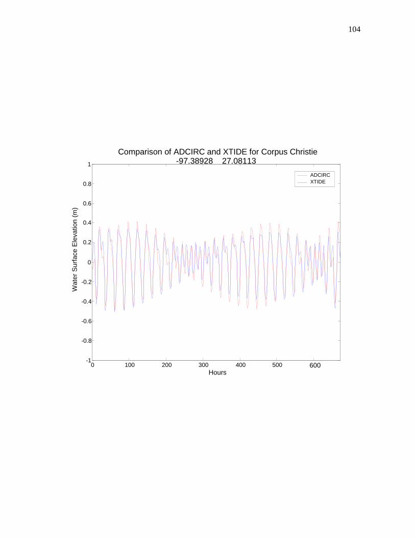
104

0 100 200 300 400 500 600 -1

-0.8

-0.6

-0.4

-0.2

0

0.2

0.4

0.6

0.8

1

Hours

Wat

er S

urfa

ce E

leva

tion

(m)

Comparison of ADCIRC and XTIDE for Corpus Christie -97.38928 27.08113

ADCIRC XTIDE

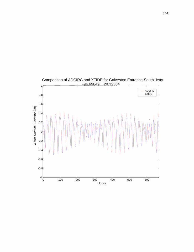
105

0 100 200 300 400 500 600 -1

-0.8

-0.6

-0.4

-0.2

0

0.2

0.4

0.6

0.8

1

Hours

Wat

er S

urfa

ce E

leva

tion

(m)

Comparison of ADCIRC and XTIDE for Galveston Entrance-South Jetty-94.69849 29.32304

ADCIRC XTIDE

106

0 100 200 300 400 500 600 -1

-0.8

-0.6

-0.4

-0.2

0

0.2

0.4

0.6

0.8

1

Hours

Wat

er S

urfa

ce E

leva

tion

Comparison of ADCIRC and XTIDE for Galveston Bay Entrance-94.70587 29.34739

ADCIRC XTIDE

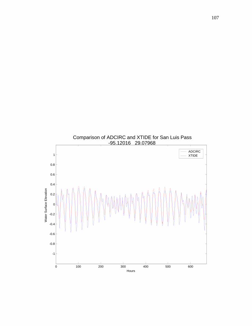
107

0 100 200 300 400 500 600

-1

-0.8

-0.6

-0.4

-0.2

0

0.2

0.4

0.6

0.8

1

Hours

Wat

er S

urfa

ce E

leva

tion

Comparison of ADCIRC and XTIDE for San Luis Pass -95.12016 29.07968

ADCIRC XTIDE

108

0 100 200 300 400 500 600 -1

-0.8

-0.6

-0.4

-0.2

0

0.2

0.4

0.6

0.8

1

Hours

Wat

er S

urfa

ce E

leva

tion

(m)

Comparison of ADCIRC and XTIDE for Sabine Pass -93.83873 29.68882

ADCIRC XTIDE

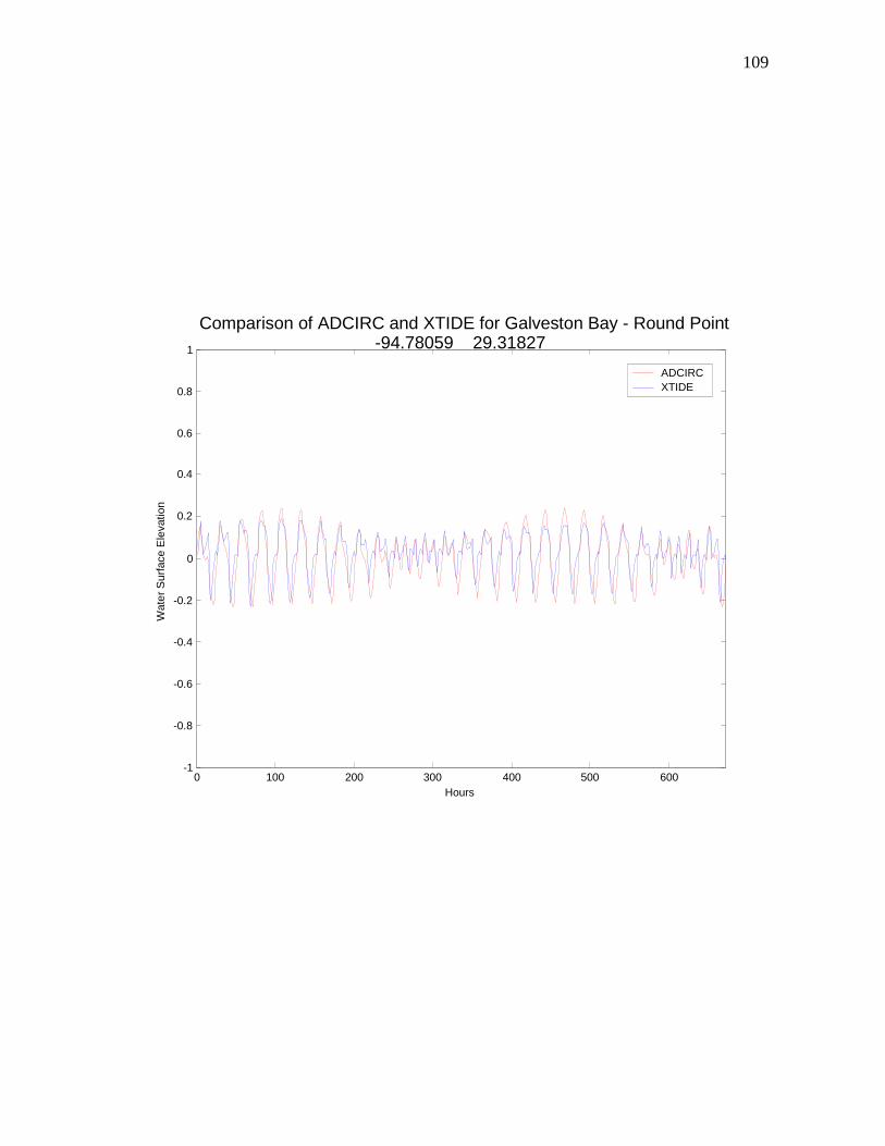
109

0 100 200 300 400 500 600 -1

-0.8

-0.6

-0.4

-0.2

0

0.2

0.4

0.6

0.8

1

Hours

Wat

er S

urfa

ce E

leva

tion

Comparison of ADCIRC and XTIDE for Galveston Bay - Round Point -94.78059 29.31827

ADCIRC XTIDE

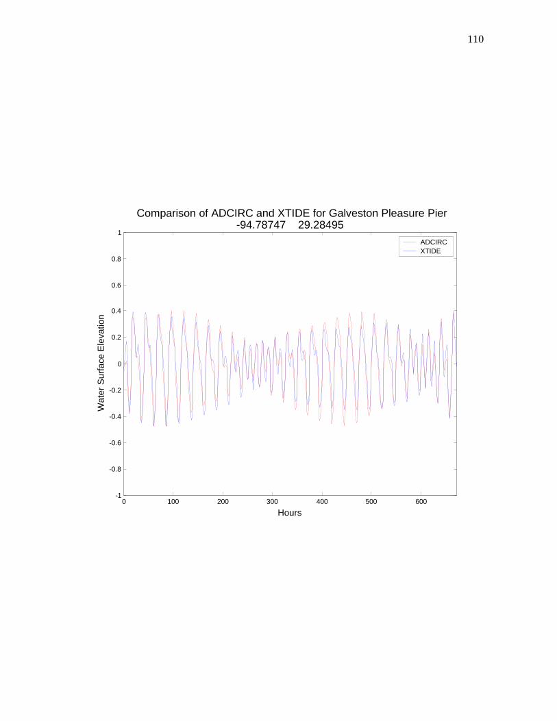
110

0 100 200 300 400 500 600 -1

-0.8

-0.6

-0.4

-0.2

0

0.2

0.4

0.6

0.8

1

Hours

Wat

er S

urfa

ce E

leva

tion

Comparison of ADCIRC and XTIDE for Galveston Pleasure Pier -94.78747 29.28495

ADCIRC XTIDE

111

0 100 200 300 400 500 600

-1

-0.8

-0.6

-0.4

-0.2

0

0.2

0.4

0.6

0.8

1

Hours

Wat

er S

urfa

ce E

leva

tion

Comparison of ADCIRC and XTIDE for Galveston Bay-Morgans P i -94.9766 29.6756

ADCIRCXTIDE

112

0 100 200 300 400 500 600

-1

-0.8

-0.6

-0.4

-0.2

0

0.2

0.4

0.6

0.8

1

Hours

Wat

er S

urfa

ce E

leva

tion

(m)

Comparison of ADCIRC and XTIDE for Lynchburg Landing, San Jacinto River-95.09607 29.77917

ADCIRC XTIDE

113

0 100 200 300 400 500 600

-1

-0.8

-0.6

-0.4

-0.2

0

0.2

0.4

0.6

0.8

1

Hours

Wat

er S

urfa

ce E

leva

tion

Comparison of ADCIRC and Xtide for Jamaica Beach -95.00899 29.19919

ADCIRC XTIDE

114

0 100 200 300 400 500 600 -1

-0.8

-0.6

-0.4

-0.2

0

0.2

0.4

0.6

0.8

1

Hours

Wat

er S

urfa

ce E

leva

tion

Comparison of ADCIRC and Xtide for Galveston Channel Entrance(2) -94.78774 29.31305

ADCIRCXTIDE

115

0 100 200 300 400 500 600 -1

-0.8

-0.6

-0.4

-0.2

0

0.2

0.4

0.6

0.8

1

Hours

Wat

er S

urfa

ce E

leva

tion

Comparison of ADCIRC and XTIDE for Galveston Channel Entrance-94.80136 29.31203

ADCIRCXTIDE

116

APPENDIX B

STORM TRACKS AND SURGE PLOTS

117

118

Storm 5( 8/24/1886) Pleasure PIer

-0.4

-0.2

0

0.2

0.4

0.6

0.8

1

0 1 2 3 4 5 6 7

Time, days from 8/24/1886

Surg

e - m

eter

sAdcirc Galveston

Storm 5( 8/24/1886) Freeport

-0.4

-0.2

0

0.2

0.4

0.6

0.8

1

1.2

0 1 2 3 4 5 6 7Time, days from 8/24/1886

Sur

ge -

met

ers

Adcirc Freeport

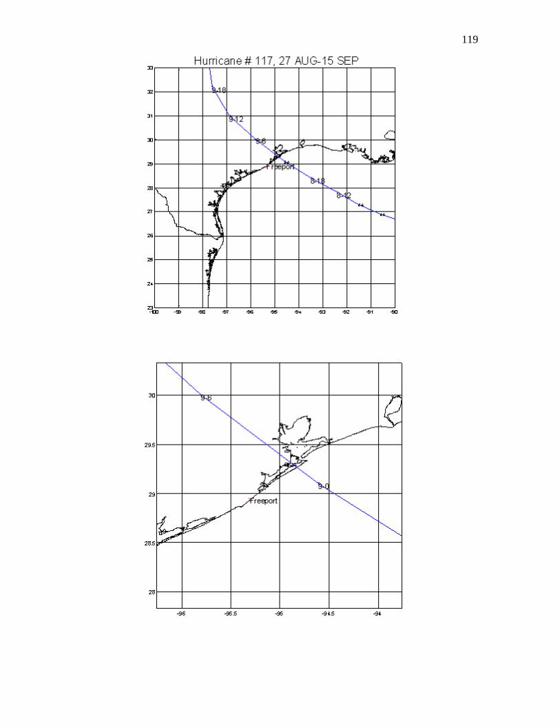
119

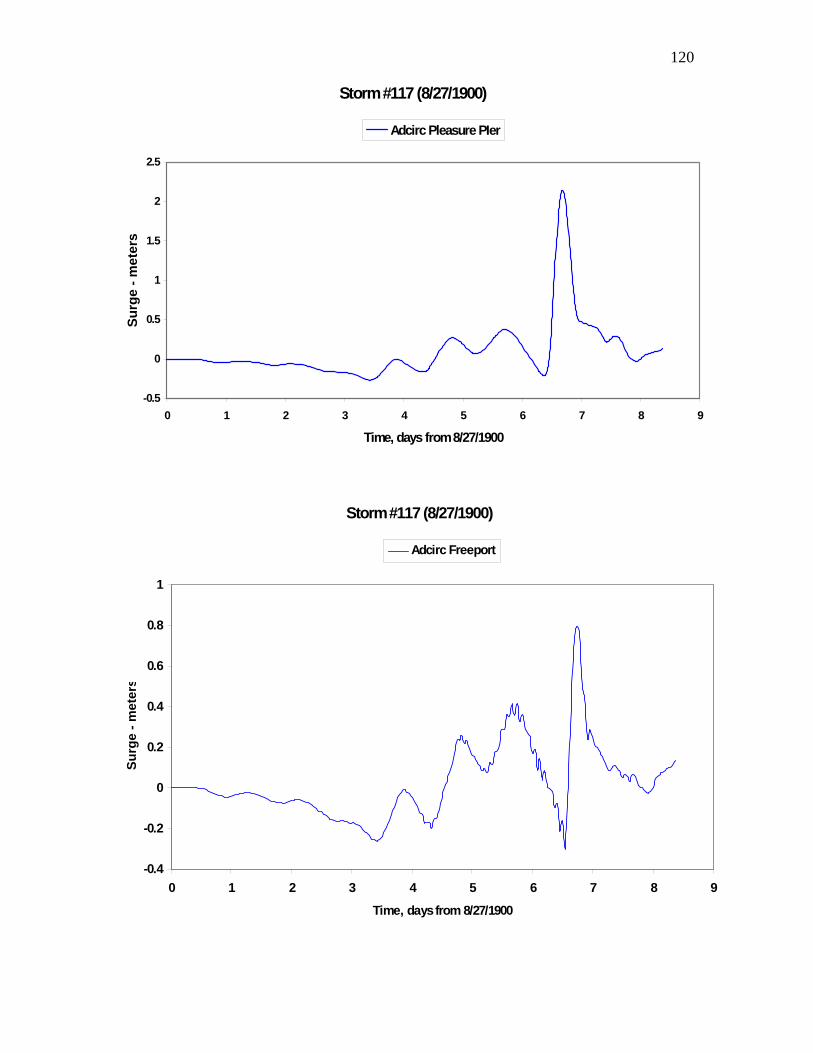
120

Storm #117 (8/27/1900)

-0.5

0

0.5

1

1.5

2

2.5

0 1 2 3 4 5 6 7 8 9

Time, days from 8/27/1900

Surg

e - m

eter

sAdcirc Pleasure PIer

Storm #117 (8/27/1900)

-0.4

-0.2

0

0.2

0.4

0.6

0.8

1

0 1 2 3 4 5 6 7 8 9

Time, days from 8/27/1900

Surg

e - m

eter

s

Adcirc Freeport

121

122

Storm 117 (+1.0) (8/27/1900)

-0.5

0

0.5

1

1.5

2

2.5

3

3.5

0 1 2 3 4 5 6 7 8 9

Time, days from 8/27/1900

Surg

e - m

eter

sAdcirc Pleasure PIer

Storm 117 (+1.0) ( 8/27/1900)

-0.5

0

0.5

1

1.5

2

2.5

3

0 1 2 3 4 5 6 7 8 9

Time, days from 8/27/1900

Surg

e - m

eter

s

Adcirc Freeport

123

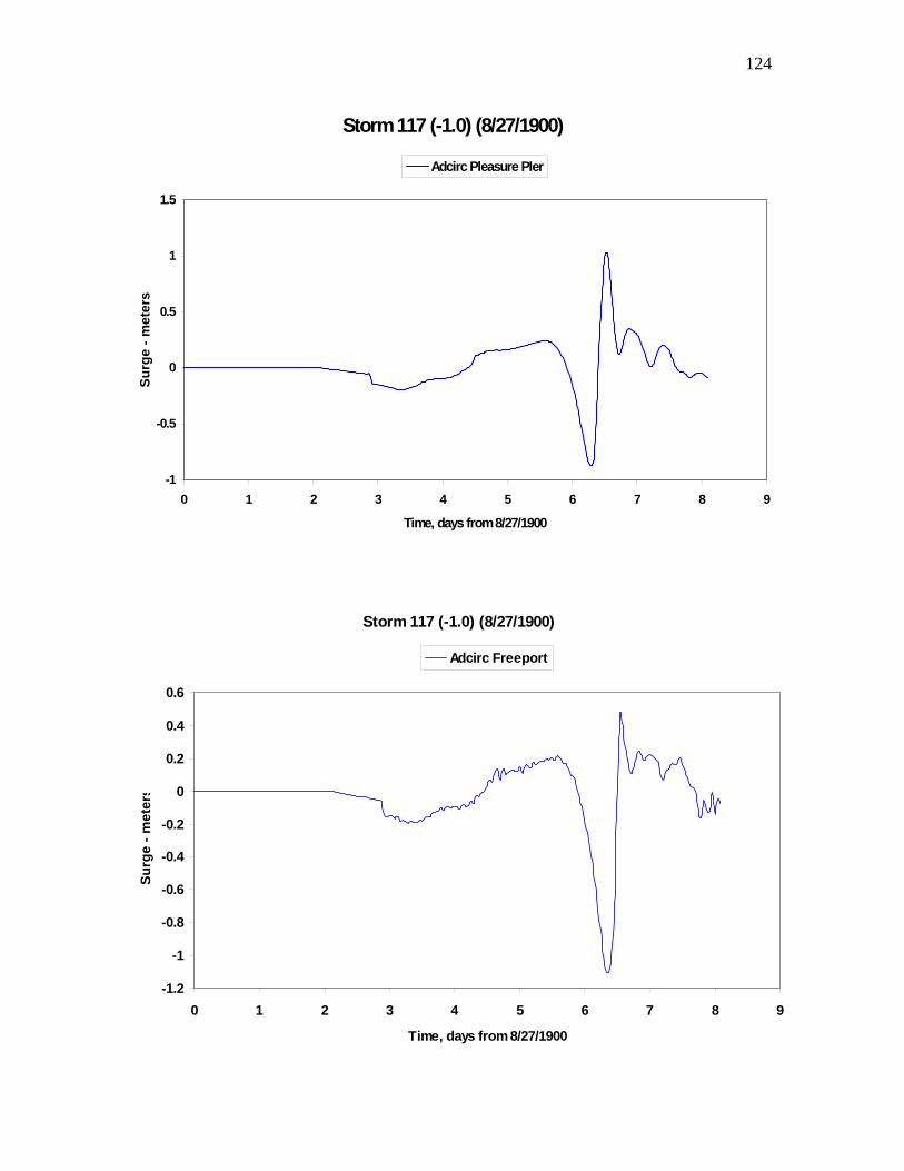
124

Storm 117 (-1.0) (8/27/1900)

-1

-0.5

0

0.5

1

1.5

0 1 2 3 4 5 6 7 8 9

Time, days from 8/27/1900

Surg

e - m

eter

sAdcirc Pleasure PIer

Storm 117 (-1.0) (8/27/1900)

-1.2

-1

-0.8

-0.6

-0.4

-0.2

0

0.2

0.4

0.6

0 1 2 3 4 5 6 7 8 9

Time, days from 8/27/1900

Surg

e - m

eter

s

Adcirc Freeport

125

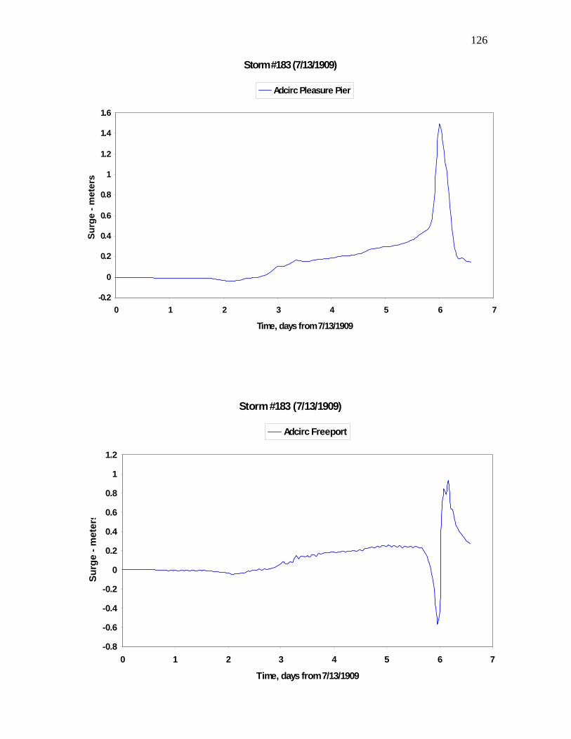
126

Storm #183 (7/13/1909)

-0.2

0

0.2

0.4

0.6

0.8

1

1.2

1.4

1.6

0 1 2 3 4 5 6 7

Time, days from 7/13/1909

Surg

e - m

eter

sAdcirc Pleasure Pier

Storm #183 (7/13/1909)

-0.8

-0.6

-0.4

-0.2

0

0.2

0.4

0.6

0.8

1

1.2

0 1 2 3 4 5 6 7

Time, days from 7/13/1909

Surg

e - m

eter

s

Adcirc Freeport

127

128

Storm 211 (8/5/1915)

-0.5

0

0.5

1

1.5

2

2.5

3

3.5

0 1 2 3 4 5 6 7 8 9Time, hours from 8/5/1915

Surg

e - m

eter

sAdcirc Pleasure Pier

Storm 211 (8/5/1915)

-0.6

-0.4

-0.2

0

0.2

0.4

0.6

0.8

1

1.2

1.4

1.6

0 1 2 3 4 5 6 7 8 9

Time, hours from 8/5/1915

Surg

e - m

eter

s

Adcirc Freeport

129

130

Storm 211 (+1.0) (8/5/1915)

-0.5

0

0.5

1

1.5

2

2.5

3

3.5

0 1 2 3 4 5 6 7 8 9

Time, hours from 8/5/1915

Surg

e - m

eter

sAdcirc Pleasure Pier

Storm 211 (+1.0) (8/5/1915)

-0.5

0

0.5

1

1.5

2

2.5

3

3.5

4

0 1 2 3 4 5 6 7 8 9

Time, hours from 8/5/1915

Surg

e - m

eter

s

Adcirc Freeport

131

132

Storm 211 (-1.0) (8/5/1915)

-1.5

-1

-0.5

0

0.5

1

1.5

2

0 1 2 3 4 5 6 7 8 9Time, hours from 8/5/1915

Surg

e - m

eter

s

Adcirc Pleasure Pier

Storm 211 (-1.0) (8/5/1915)

-1.2

-1

-0.8

-0.6

-0.4

-0.2

0

0.2

0.4

0.6

0 1 2 3 4 5 6 7 8 9

Time, hours from 8/5/1915

Surg

e - m

eter

s

Adcirc Freeport

133

-100 -99 -98 -97 -96 -95 -94 -93 -92 -91 -90 23

24

25

26

27

28

29

30

31

32

33

Freeport

#232 , 1-7 AUG

6-6

6-12

6-18

7-0

7-6

-95.5 -95 -94.5 -94 -93.5

28.5

29

29.5

30

30.5

Freeport

7-0

134

Storm 232 (8/1/1918)

-0.8

-0.6

-0.4

-0.2

0

0.2

0.4

0.6

0.8

1

0 0.5 1 1.5 2 2.5 3 3.5 4 4.5Time, days from 8/1/1918

Surg

e - m

eter

sAdcirc Pleasure PIer

Storm 232 (8/1/1918)

-0.6

-0.4

-0.2

0

0.2

0.4

0.6

0 0.5 1 1.5 2 2.5 3 3.5 4 4.5Time, days from 8/1/1918

Surg

e - m

eter

s

Adcirc Freeport

135

136

Storm 295 (6/27/1929)

-0.1

0

0.1

0.2

0.3

0.4

0.5

0.6

0.7

0.8

0.9

0 0.5 1 1.5 2 2.5Time, days from 6/27/1929

Surg

e - m

eter

sAdcirc Pleasure Pier

Storm 295 (6/27/1929)

-0.2

0

0.2

0.4

0.6

0.8

1

1.2

0 0.5 1 1.5 2 2.5Time, days from 6/27/1929

Surg

e - m

eter

s

Adcirc Freeport

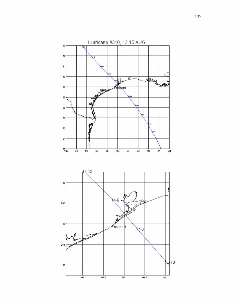
137

138

Storm 310 (8/12/1932)

0

0.5

1

1.5

2

2.5

3

3.5

0 0.5 1 1.5 2 2.5 3 3.5

Time, days from 8/12/1932

Surg

e - m

eter

sAdcirc Pleasure PIer

Storm 310 (8/12/1932)

-2

-1.5

-1

-0.5

0

0.5

1

0 0.5 1 1.5 2 2.5 3 3.5Time, days from 8/12/1932

Surg

e - m

eter

s

Adcirc Freeport

139

140

Storm 310 (+1.0) (8/12/1932)

0

0.2

0.4

0.6

0.8

1

1.2

1.4

1.6

1.8

2

0 0.5 1 1.5 2 2.5 3 3.5Time, days from 8/12/1932

Surg

e - m

eter

sAdcirc Pleasure PIer

Storm 310 (+1.0) (8/12/1932)

0

0.5

1

1.5

2

2.5

3

3.5

0 0.5 1 1.5 2 2.5 3 3.5

Time, days from 8/12/1932

Surg

e - m

eter

s

Adcirc Freeport

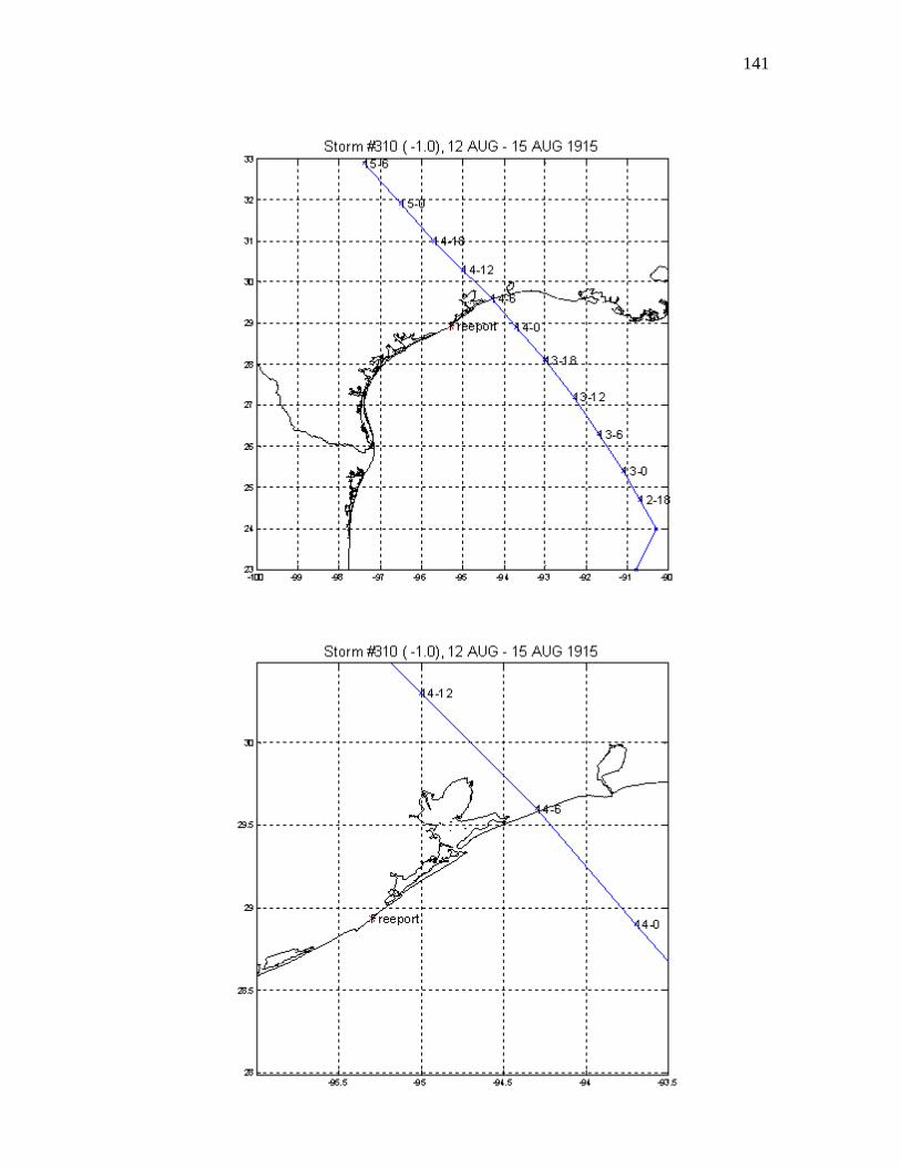
141

142

Storm 310 (-1.0) (8/12/1932)

-0.4

-0.3

-0.2

-0.1

0

0.1

0.2

0.3

0.4

0.5

0.6

0.7

0 0.5 1 1.5 2 2.5 3 3.5Time, days from 8/12/1932

Surg

e - m

eter

sAdcirc Pleasure PIer

Storm 310 (-1.0) (8/12/1932)

-0.2

-0.1

0

0.1

0.2

0.3

0.4

0.5

0 0.5 1 1.5 2 2.5 3 3.5

Time, days from 8/12/1932

Surg

e - m

eter

s

Adcirc Freeport

143

144

Storm 324(7/25/1933)

-0.1

0

0.1

0.2

0.3

0.4

0.5

0.6

0.7

0.8

0 1 2 3 4 5 6 7 8

Time, days from 7/25/1933

Surg

e - m

eter

sAdcirc Pleasure PIer

Storm 324(7/25/1933)

-0.1

0

0.1

0.2

0.3

0.4

0.5

0.6

0 1 2 3 4 5 6 7 8

Time, days from 7/25/1933

Surg

e - m

eter

s

Adcirc Freeport

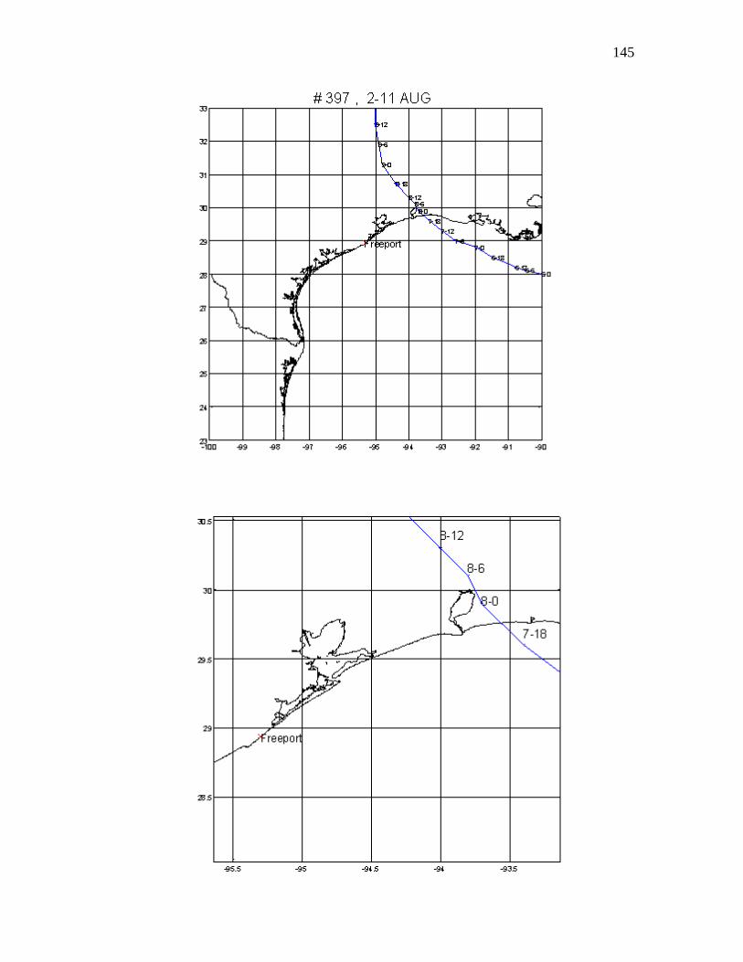
145

146

Storm 397 (8/2/1940)

-0.7

-0.6

-0.5

-0.4

-0.3

-0.2

-0.1

0

0.1

0.2

0.3

0.4

0 1 2 3 4 5 6 7 8 9 10

Time, days from 8/2/1940

Surg

e - m

eter

sAdcirc Pleasure PIer

Storm 397 (8/2/1940)

-0.6

-0.5

-0.4

-0.3

-0.2

-0.1

0

0.1

0.2

0.3

0 1 2 3 4 5 6 7 8 9 10

Time, days from 8/2/1940

Surg

e -

Adcirc Freeport

147

148

Storm 405 (9/16/1941)

-0.5

0

0.5

1

1.5

2

2.5

0 1 2 3 4 5 6 7 8 9Time, days from 9/16/1941

Surg

e - m

eter

sAdcirc Pleasure PIer

Storm 405 (9/16/1941)

-0.5

0

0.5

1

1.5

2

2.5

0 1 2 3 4 5 6 7 8 9

Time, days from 9/16/1941

Surg

e - m

eter

s

Adcirc Freeport

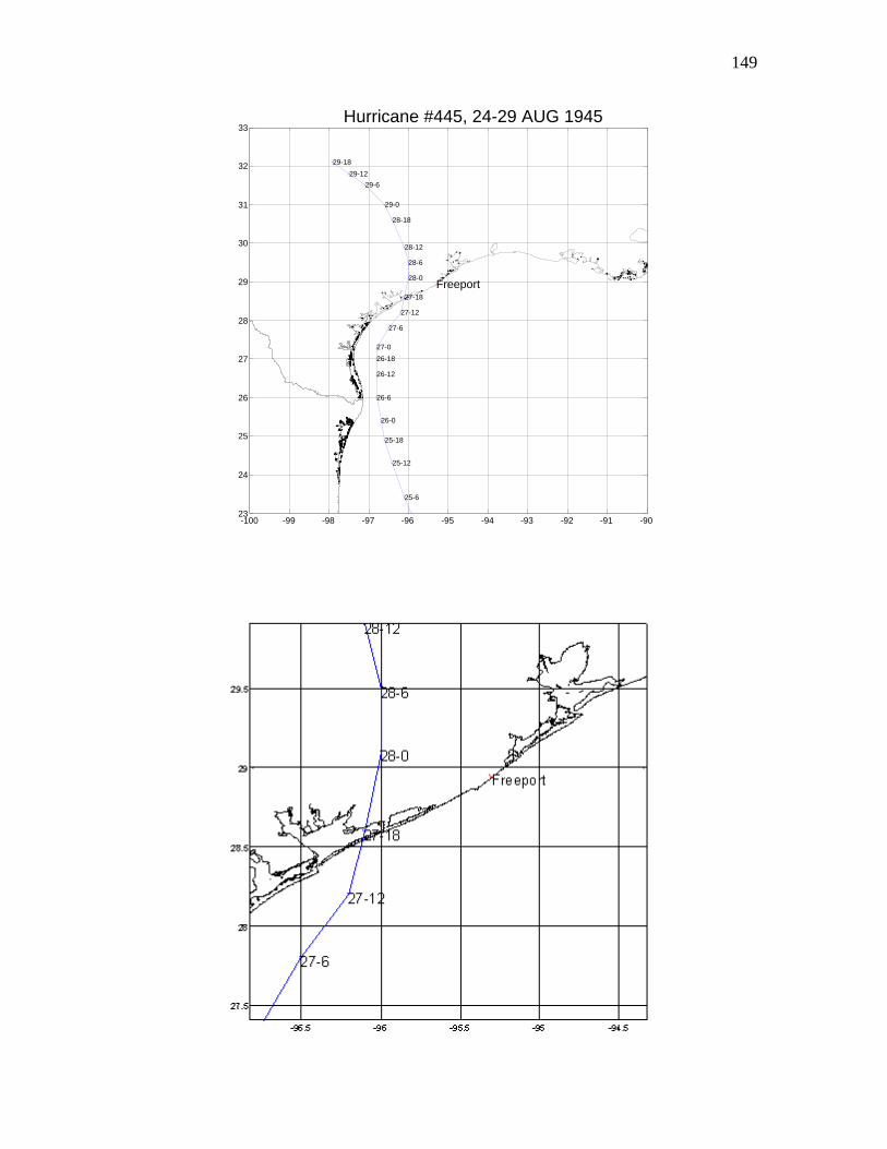
149

-100 -99 -98 -97 -96 -95 -94 -93 -92 -91 -9023

24

25

26

27

28

29

30

31

32

33

Freeport

Hurricane #445, 24-29 AUG 1945

25-6

25-12

25-18

26-0

26-6

26-12

26-1827-0

27-6

27-12

27-18

28-0

28-6

28-12

28-18

29-0

29-629-12

29-18

150

Storm 445( 8/24/1945)

-0.2

0

0.2

0.4

0.6

0.8

1

1.2

0 1 2 3 4 5 6

Time, days from 8/24/1945

Surg

e - m

eter

sAdcirc Pleasure Pier

Storm 445( 8/24/1945)

-0.2

0

0.2

0.4

0.6

0.8

1

1.2

1.4

1.6

0 1 2 3 4 5 6

Time, days from 8/24/1945

Surg

e - m

eter

s

Adcirc Freeport

151

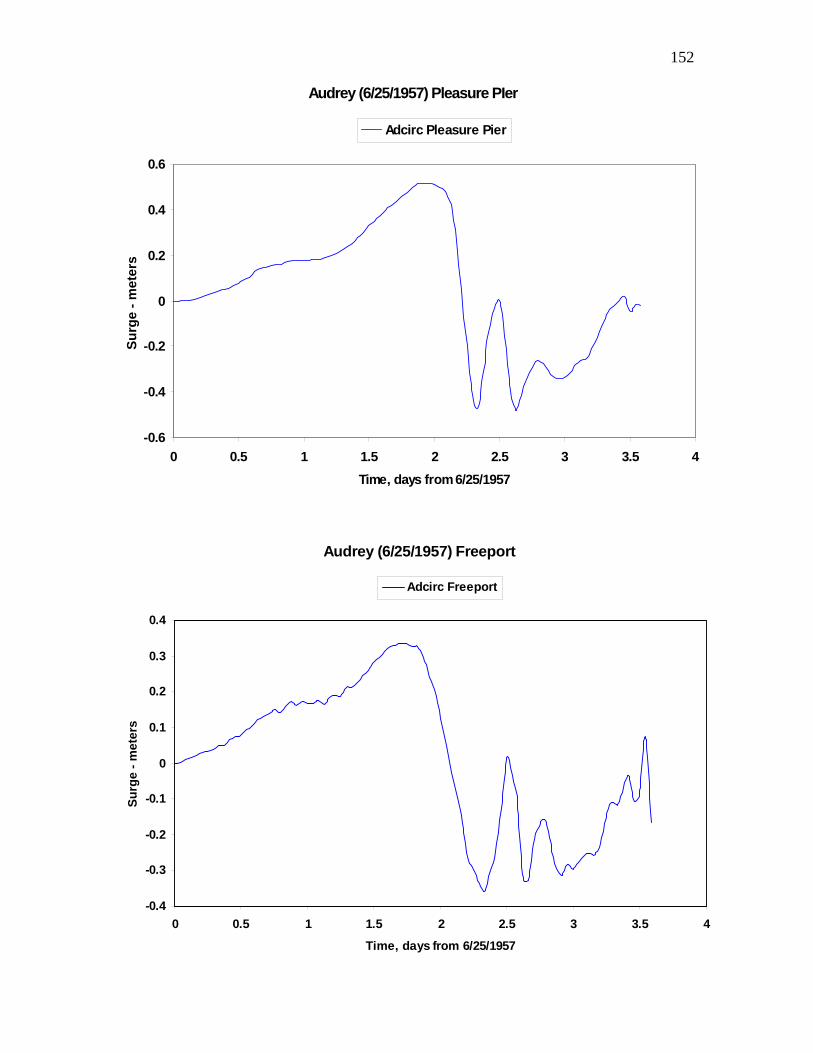
152

Audrey (6/25/1957) Pleasure PIer

-0.6

-0.4

-0.2

0

0.2

0.4

0.6

0 0.5 1 1.5 2 2.5 3 3.5 4Time, days from 6/25/1957

Surg

e - m

eter

sAdcirc Pleasure Pier

Audrey (6/25/1957) Freeport

-0.4

-0.3

-0.2

-0.1

0

0.1

0.2

0.3

0.4

0 0.5 1 1.5 2 2.5 3 3.5 4

Time, days from 6/25/1957

Surg

e - m

eter

s

Adcirc Freeport

153

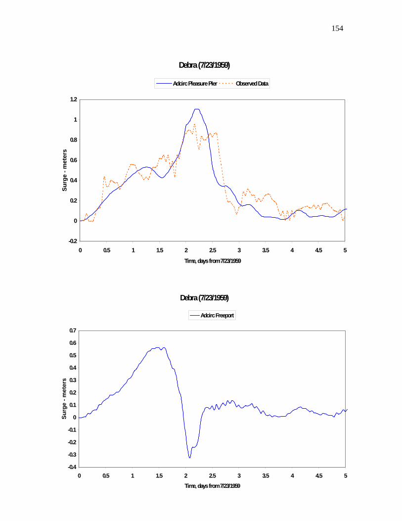
154

Debra (7/23/1959)

-0.2

0

0.2

0.4

0.6

0.8

1

1.2

0 0.5 1 1.5 2 2.5 3 3.5 4 4.5 5

Time, days from 7/23/1959

Surg

e - m

eter

s

Adcirc Pleasure PIer Observed Data

Debra (7/23/1959)

-0.4

-0.3

-0.2

-0.1

0

0.1

0.2

0.3

0.4

0.5

0.6

0.7

0 0.5 1 1.5 2 2.5 3 3.5 4 4.5 5

Time, days from 7/23/1959

Surg

e - m

eter

s

Adcirc Freeport

155

156

Carla (9/3/1961)

-0.5

0

0.5

1

1.5

2

2.5

0 2 4 6 8 10 12 14 16

Time, days from 9/3/1961

Surg

e - m

eter

sAdcirc Pleasure Pier Observed Data

Carla (9/3/1961)

-0.5

0

0.5

1

1.5

2

2.5

3

3.5

0 2 4 6 8 10 12 14 16

Time, days from 9/3/1961

Surg

e - m

eter

s

Adcirc Freeport

157

158

Carla (+1.0) (9/3/1961)

-0.2

0

0.2

0.4

0.6

0.8

1

1.2

0 1 2 3 4 5 6 7 8 9 10

Time, days from 9/3/1961

Surg

e - m

eter

sAdcirc Pleasure Pier

Carla (+1.0) (9/3/1961)

-0.5

0

0.5

1

1.5

2

0 1 2 3 4 5 6 7 8 9 10Time, days from 9/3/1961

Surg

e - m

eter

s

Adcirc Freeport

159

160

Carla (-1.0) (9/3/1961)

-0.5

0

0.5

1

1.5

2

2.5

3

3.5

4

0 1 2 3 4 5 6 7 8 9 10 11

Time, days from 9/3/1961

Surg

e - m

eter

sAdcirc Pleasure Pier

Carla (-1.0) (9/3/1961)

-0.5

0

0.5

1

1.5

2

2.5

3

3.5

4

4.5

5

0 1 2 3 4 5 6 7 8 9 10 11

Time, days from 9/3/1961

Surg

e - m

eter

s

Adcirc Freeport

161

162

Celia (7/31/1970)

-0.2

0

0.2

0.4

0.6

0.8

1

1.2

0 1 2 3 4 5 6

Time, days from 7/31/1970

Surg

e - m

eter

sAdcirc Pleasure PIer Observed Data

Celia (7/31/1970)

-0.2

0

0.2

0.4

0.6

0.8

1

1.2

1.4

1.6

1.8

0 1 2 3 4 5 6

Time, days from 7/31/1970

Surg

e - m

eter

s

Adcirc Freeport

163

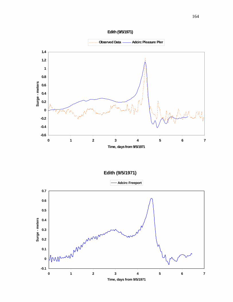
164

Edith (9/5/1971)

-0.6

-0.4

-0.2

0

0.2

0.4

0.6

0.8

1

1.2

1.4

0 1 2 3 4 5 6 7

Time, days from 9/5/1971

Surg

e - m

eter

sObserved Data Adcirc Pleasure PIer

Edith (9/5/1971)

-0.1

0

0.1

0.2

0.3

0.4

0.5

0.6

0.7

0 1 2 3 4 5 6 7Time, days from 9/5/1971

Surg

e - m

eter

s

Adcirc Freeport

165

166

Fern (9/3/1971)

-0.6

-0.4

-0.2

0

0.2

0.4

0.6

0.8

1

1.2

1.4

1.6

0 1 2 3 4 5 6 7 8 9Time, days from 9/3/1971

Surg

e - m

eter

sObserved Data Adcirc Pleasure PIer

Fern (9/3/1971)

-0.5

0

0.5

1

1.5

2

0 1 2 3 4 5 6 7 8 9Time, days from 9/3/1971

Surg

e - m

eter

s

Adcirc Freeport

167

168

Delia (9/1/1973)

-0.2

0

0.2

0.4

0.6

0.8

1

1.2

1.4

0 1 2 3 4 5

Time, days from 9/1/1973

Surg

e - m

eter

sObserved Data Adcirc Pleasure PIer

Delia (9/1/1973)

-0.6

-0.4

-0.2

0

0.2

0.4

0.6

0.8

1

1.2

0 1 2 3 4 5

Time, days from 9/1/1973

Surg

e - m

eter

s

Adcirc Freeport

169

170

Chris (9/9/1982)

-0.3

-0.2

-0.1

0

0.1

0.2

0.3

0.4

0.5

0 1 2 3 4Time, days from 9/9/1982

Surg

e - m

eter

sObserved data Pleasure Pier Adcirc Pleasure Pier

Chris (9/9/1982)

-0.2

-0.1

0

0.1

0.2

0.3

0.4

0 1 2 3 4Time, days from 9/9/1982

Surg

e - m

eter

s

Adcirc Freeport

171

172

Alicia (8/15/1983)

-0.5

0

0.5

1

1.5

2

2.5

3

0 0.5 1 1.5 2 2.5 3 3.5 4 4.5 5

Time, days from 8/15/1983

Surg

e - m

eter

sObserved Data Adcirc Pleasure Pier

Alicia (8/15/1983)

-0.2

0

0.2

0.4

0.6

0.8

1

1.2

0 0.5 1 1.5 2 2.5 3 3.5 4 4.5 5

Time, days from 8/15/1983

Surg

e - m

eter

s

Adcirc Freeport

173

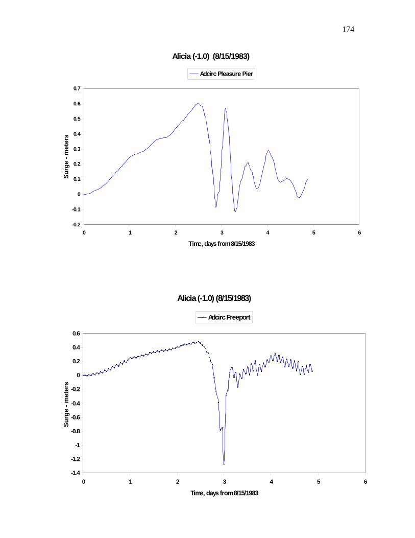
174

Alicia (-1.0) (8/15/1983)

-0.2

-0.1

0

0.1

0.2

0.3

0.4

0.5

0.6

0.7

0 1 2 3 4 5 6

Time, days from 8/15/1983

Surg

e - m

eter

sAdcirc Pleasure Pier

Alicia (-1.0) (8/15/1983)

-1.4

-1.2

-1

-0.8

-0.6

-0.4

-0.2

0

0.2

0.4

0.6

0 1 2 3 4 5 6

Time, days from 8/15/1983

Surg

e - m

eter

s

Adcirc Freeport

175

176

Alicia (+1.0) (8/15/1983)

0

0.2

0.4

0.6

0.8

1

1.2

0 1 2 3 4 5

Time, days from 8/15/1983

Surg

e - m

eter

sAdcirc Pleasure Pier

Alicia (+1.0) (8/15/1983)

0

0.2

0.4

0.6

0.8

1

1.2

0 1 2 3 4 5

Time, days from 8/15/1983

Surg

e - m

eter

s

Adcirc Freeport

177

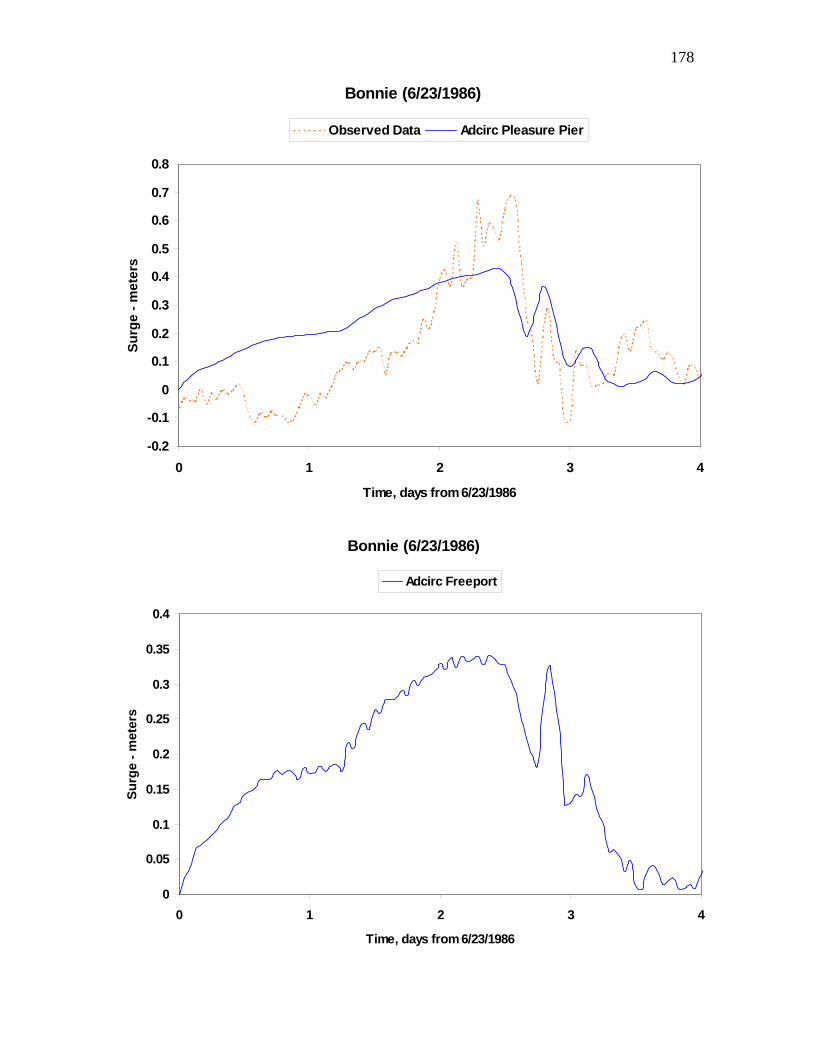
178

Bonnie (6/23/1986)

-0.2

-0.1

0

0.1

0.2

0.3

0.4

0.5

0.6

0.7

0.8

0 1 2 3 4

Time, days from 6/23/1986

Surg

e - m

eter

sObserved Data Adcirc Pleasure Pier

Bonnie (6/23/1986)

0

0.05

0.1

0.15

0.2

0.25

0.3

0.35

0.4

0 1 2 3 4

Time, days from 6/23/1986

Surg

e - m

eter

s

Adcirc Freeport

179

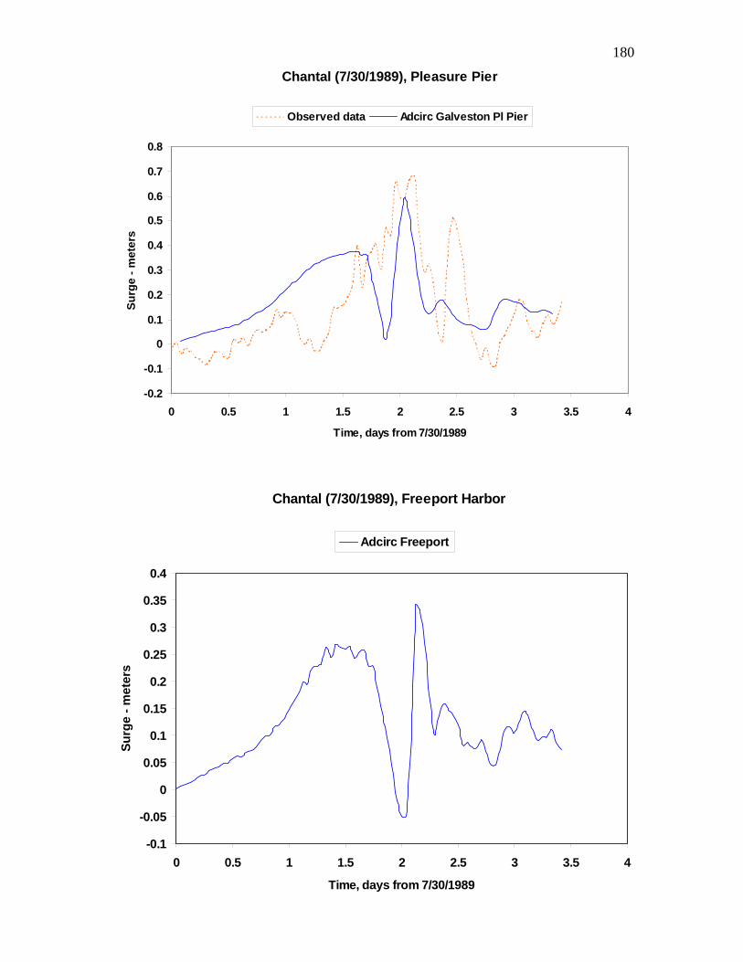
180

Chantal (7/30/1989), Pleasure Pier

-0.2

-0.1

0

0.1

0.2

0.3

0.4

0.5

0.6

0.7

0.8

0 0.5 1 1.5 2 2.5 3 3.5 4

Time, days from 7/30/1989

Surg

e - m

eter

sObserved data Adcirc Galveston Pl Pier

Chantal (7/30/1989), Freeport Harbor

-0.1

-0.05

0

0.05

0.1

0.15

0.2

0.25

0.3

0.35

0.4

0 0.5 1 1.5 2 2.5 3 3.5 4

Time, days from 7/30/1989

Surg

e - m

eter

s

Adcirc Freeport

181

182

Jerry (10/12/1989)

-0.2

0

0.2

0.4

0.6

0.8

1

1.2

1.4

1.6

0 1 2 3 4Time, days from 10/12/1989

Surg

e - m

eter

sObserved Data Adcirc Pleasure Pier

Jerry (10/12/1989)

-0.2

0

0.2

0.4

0.6

0.8

1

1.2

0 1 2 3 4

Time, days from 10/12/1989

Surg

e - m

eter

s

Adcirc Freeport

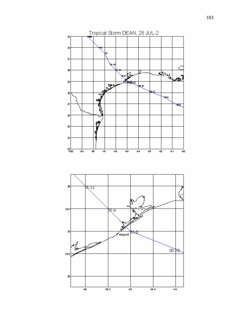
183

184

Dean (7/28/1995), Pleasure Pier

-0.4

-0.2

0

0.2

0.4

0.6

0.8

1

0 1 2 3 4 5 6

Time, days from 7/28/1995

Surg

e - m

eter

sObserved Data Adcirc Pleasure PIer

Dean (7/28/1995), Freeport Harbor

-0.1

0

0.1

0.2

0.3

0.4

0.5

0 1 2 3 4 5 6Time, days from 7/28/1995

Surg

e - m

eter

s

Adcirc Freeport

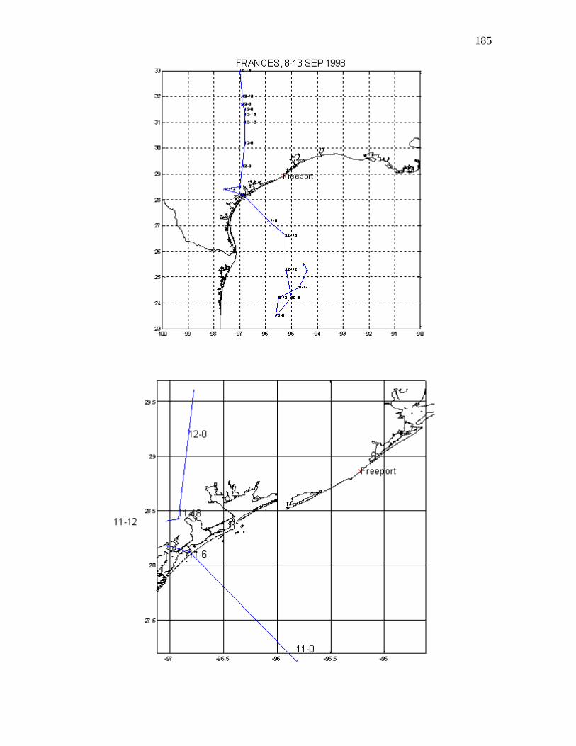
185

186

Frances (9/8/1998)

-0.2

0

0.2

0.4

0.6

0.8

1

0 1 2 3 4

Time, days from 9/8/1998

Surg

e - m

eter

sObserved Data Adcirc Pleasure Pier

Frances (9/8/1998)

-0.2

0

0.2

0.4

0.6

0.8

1

0 1 2 3 4

Time, days from 9/8/1998

Surg

e - m

eter

s

Adcirc Freeport Observed Data

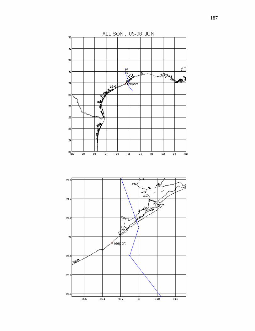
187

188

Allison (6/5/2001)

-0.4

-0.2

0

0.2

0.4

0.6

0.8

1

0 1 2 3 4 5 6 7 8 9 10Time, days from 6/5/2001

Surg

e - m

eter

sObserved Data Adcirc Pleasure Pier

Allison (6/5/2001)

-0.3

-0.2

-0.1

0

0.1

0.2

0.3

0.4

0.5

0.6

0.7

0 1 2 3 4 5 6 7 8 9 10Time, days from 6/5/2001

Surg

e - m

eter

s

Observed Data Adcirc Freeport

189

190

Claudette (7/9/2003)

-0.4

-0.2

0

0.2

0.4

0.6

0.8

1

1.2

1.4

1.6

1.8

0 1 2 3 4 5 6 7

Time, days from 7/9/2003

Surg

e - m

eter

sObserved Data Adcirc Pleasure Pier

Claudette (7/9/2003)

-0.5

0

0.5

1

1.5

2

0 1 2 3 4 5 6 7

Time, days from 7/9/2003

Surg

e - m

eter

s

Observed Data Adcirc Freeport

191

APPENDIX C

STORM SURGE FREQUENCY-OF-OCCURRENCE RELATIONSHIPS

192

Figure: Location of points used for input to EST model

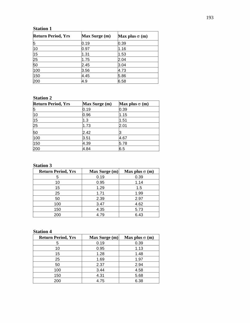
193

Station 1 Return Period, Yrs Max Surge (m) Max plus σ (m) 5 0.19 0.39 10 0.97 1.16 15 1.31 1.53 25 1.75 2.04 50 2.45 3.04 100 3.56 4.73 150 4.45 5.86 200 4.9 6.58 Station 2 Return Period, Yrs Max Surge (m) Max plus σ (m) 5 0.19 0.39 10 0.96 1.15 15 1.3 1.51 25 1.73 2.01

50 2.42 3 100 3.51 4.67 150 4.39 5.78 200 4.84 6.5 Station 3

Return Period, Yrs Max Surge (m) Max plus σ (m) 5 0.19 0.39 10 0.95 1.14 15 1.29 1.5 25 1.71 1.99 50 2.39 2.97

100 3.47 4.62 150 4.35 5.73 200 4.79 6.43

Station 4

Return Period, Yrs Max Surge (m) Max plus σ (m) 5 0.19 0.39 10 0.95 1.13 15 1.28 1.48 25 1.69 1.97 50 2.37 2.94

100 3.44 4.58 150 4.31 5.68 200 4.75 6.38

194

Station 5 Return Period, Yrs Max Surge (m) Max plus σ (m)

5 0.19 0.39 10 0.94 1.13 15 1.27 1.47 25 1.68 1.96 50 2.35 2.92

100 3.42 4.56 150 4.29 5.65 200 4.73 6.35

Station 6

Return Period, Yrs Max Surge (m) Max plus σ (m) 5 0.19 0.4 10 0.94 1.12 15 1.27 1.47 25 1.67 1.95 50 2.35 2.92

100 3.42 4.56 150 4.28 5.64 200 4.72 6.34

Station 7

Return Period, Yrs Max Surge (m) Max plus σ (m) 5 0.19 0.4 10 0.94 1.12 15 1.27 1.47 25 1.67 1.95 50 2.35 2.92

100 3.42 4.56 150 4.29 5.65 200 4.73 6.35

Station 8

Return Period, Yrs Max Surge (m) Max plus σ (m) 5 0.19 0.4 10 0.94 1.12 15 1.27 1.47 25 1.67 1.95 50 2.34 2.92

100 3.42 4.57 150 4.29 5.66 200 4.73 6.36

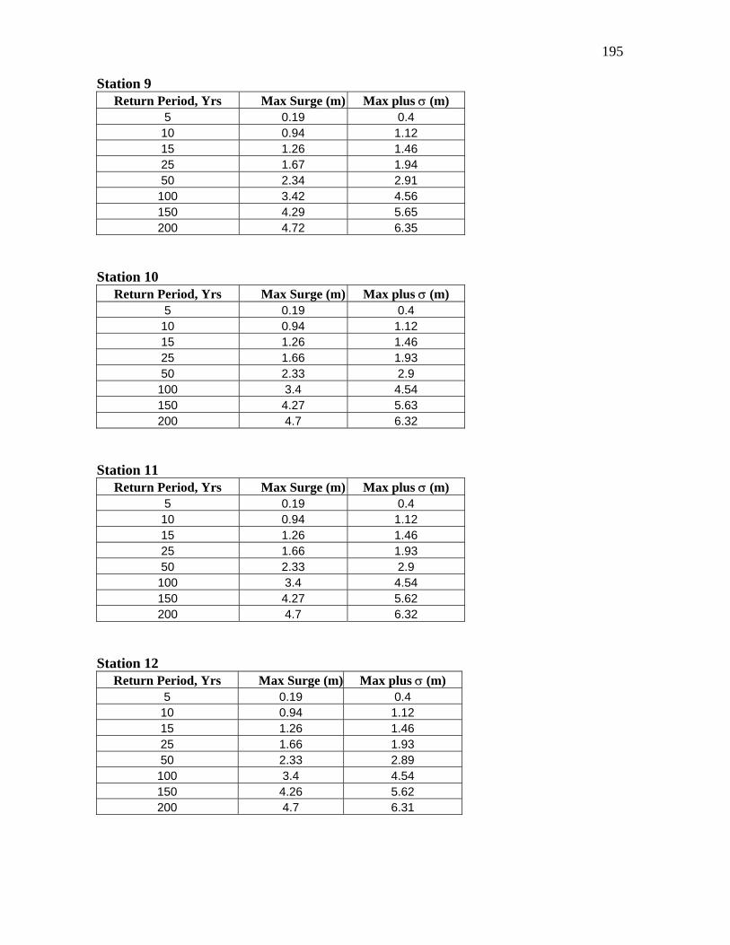
195

Station 9 Return Period, Yrs Max Surge (m) Max plus σ (m)

5 0.19 0.4 10 0.94 1.12 15 1.26 1.46 25 1.67 1.94 50 2.34 2.91

100 3.42 4.56 150 4.29 5.65 200 4.72 6.35

Station 10

Return Period, Yrs Max Surge (m) Max plus σ (m) 5 0.19 0.4 10 0.94 1.12 15 1.26 1.46 25 1.66 1.93 50 2.33 2.9

100 3.4 4.54 150 4.27 5.63 200 4.7 6.32

Station 11

Return Period, Yrs Max Surge (m) Max plus σ (m) 5 0.19 0.4 10 0.94 1.12 15 1.26 1.46 25 1.66 1.93 50 2.33 2.9

100 3.4 4.54 150 4.27 5.62 200 4.7 6.32

Station 12

Return Period, Yrs Max Surge (m) Max plus σ (m) 5 0.19 0.4 10 0.94 1.12 15 1.26 1.46 25 1.66 1.93 50 2.33 2.89

100 3.4 4.54 150 4.26 5.62 200 4.7 6.31

196

Station 13 Return Period, Yrs Max Surge (m) Max plus σ (m)

5 0.19 0.39 10 0.94 1.11 15 1.25 1.45 25 1.65 1.92 50 2.31 2.88 100 3.38 4.52 150 4.24 5.6 200 4.68 6.29

Station 14

Return Period, Yrs Max Surge (m) Max plus σ (m) 5 0.19 0.39 10 0.93 1.11 15 1.25 1.44 25 1.64 1.9 50 2.29 2.85

100 3.35 4.48 150 4.2 5.54 200 4.63 6.22

Station 15

Return Period, Yrs Max Surge (m) Max plus σ (m) 5 0.19 0.39 10 0.94 1.12 15 1.26 1.45 25 1.65 1.91 50 2.3 2.87

100 3.37 4.49 150 4.22 5.56 200 4.65 6.25

Station 16

Return Period, Yrs Max Surge (m) Max plus σ (m) 5 0.19 0.39 10 0.94 1.12 15 1.27 1.46 25 1.66 1.92 50 2.32 2.89

100 3.39 4.52 150 4.25 5.59 200 4.68 6.28

197

Station 17 Return Period, Yrs Max Surge (m) Max plus σ (m)

5 0.19 0.39 10 0.95 1.13 15 1.28 1.48 25 1.67 1.95 50 2.34 2.91

100 3.42 4.55 150 4.28 5.63 200 4.71 6.33

Station 18

Return Period, Yrs Max Surge (m) Max plus σ (m) 5 0.19 0.39 10 0.96 1.14 15 1.29 1.49 25 1.68 1.95 50 2.35 2.93

100 3.44 4.59 150 4.31 5.68 200 4.75 6.38

Station 19

Return Period, Yrs Max Surge (m) Max plus σ (m) 5 0.19 0.39 10 0.97 1.16 15 1.31 1.52 25 1.72 1.99 50 2.39 2.98

100 3.5 4.66 150 4.38 5.78 200 4.83 6.49

Station 20

Return Period, Yrs Max Surge (m) Max plus σ (m) 5 0.2 0.4 10 0.98 1.16 15 1.32 1.53 25 1.73 2.01 50 2.42 3.02

100 3.55 4.73 150 4.45 5.86 200 4.9 6.58

198

Station 21 Return Period, Yrs Max Surge (m) Max plus σ (m)

5 0.2 0.4 10 0.98 1.17 15 1.33 1.54 25 1.75 2.04 50 2.46 3.06

100 3.6 4.79 150 4.51 5.93 200 4.96 6.67

Station 22

Return Period, Yrs Max Surge (m) Max plus σ (m) 5 0.19 0.39 10 1.01 1.22 15 1.41 1.66 25 1.9 2.23 50 2.63 3.21

100 3.72 4.86 150 4.6 5.98 200 5.04 6.69

Station 23

Return Period, Yrs Max Surge (m) Max plus σ (m) 5 0.18 0.39 10 1.03 1.25 15 1.45 1.71 25 1.97 2.31 50 2.71 3.3

100 3.81 4.96 150 4.69 6.07 200 5.14 6.78

Station 24

Return Period, Yrs Max Surge (m) Max plus σ (m) 5 0.18 0.38 10 1.03 1.25 15 1.46 1.73 25 2.01 2.36 50 2.77 3.37

100 3.87 5.03 150 4.77 6.17 200 5.22 6.89

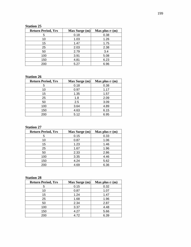
199

Station 25

Return Period, Yrs Max Surge (m) Max plus σ (m) 5 0.18 0.38 10 1.03 1.26 15 1.47 1.75 25 2.03 2.38 50 2.79 3.4

100 3.91 5.08 150 4.81 6.23 200 5.27 6.96

Station 26

Return Period, Yrs Max Surge (m) Max plus σ (m) 5 0.18 0.38 10 0.97 1.17 15 1.35 1.57 25 1.8 2.09 50 2.5 3.09

100 3.64 4.89 150 4.63 6.15 200 5.12 6.95

Station 27

Return Period, Yrs Max Surge (m) Max plus σ (m) 5 0.15 0.33 10 0.87 1.06 15 1.23 1.46 25 1.67 1.96 50 2.33 2.86

100 3.35 4.46 150 4.24 5.62 200 4.69 6.36

Station 28

Return Period, Yrs Max Surge (m) Max plus σ (m) 5 0.15 0.32 10 0.87 1.07 15 1.24 1.47 25 1.68 1.96 50 2.34 2.87

100 3.37 4.48 150 4.27 5.66 200 4.72 6.39

200

Station 29

Return Period, Yrs Max Surge (m) Max plus σ (m) 5 0.14 0.31 10 0.89 1.1 15 1.3 1.54 25 1.76 2.05 50 2.43 2.97

100 3.48 4.62 150 4.41 5.83 200 4.87 6.6

Station 30 Return Period, Yrs Max Surge (m) Max plus σ (m)

5 0.16 0.37 10 1.06 1.31 15 1.55 1.84 25 2.09 2.43 50 2.78 3.35

100 3.86 5.08 150 4.85 6.37 200 5.35 7.17

Station 31

Return Period, Yrs Max Surge (m) Max plus σ (m) 5 0.16 0.37 10 1.07 1.32 15 1.56 1.86 25 2.13 2.47 50 2.83 3.41

100 3.92 5.14 150 4.92 6.44 200 5.42 7.26

Station 32

Return Period, Yrs Max Surge (m) Max plus σ (m) 5 0.16 0.36

10 1.08 1.33 15 1.58 1.89 25 2.17 2.52 50 2.9 3.47 100 3.98 5.18 150 4.97 6.48 200 5.47 7.29

201

Station 33

Return Period, Yrs Max Surge (m) Max plus σ (m) 5 0.18 0.38

10 0.97 1.16 15 1.33 1.55 25 1.77 2.07 50 2.5 3.12 100 3.67 4.94 150 4.65 6.19 200 5.15 6.98

Station 34

Return Period, Yrs Max Surge (m) Max plus σ (m) 5 0.19 0.39

10 0.99 1.19 15 1.35 1.58 25 1.79 2.08 50 2.52 3.13 100 3.69 4.95 150 4.67 6.21 200 5.17 7.02

Station 35

Return Period, Yrs Max Surge (m) Max plus σ (m) 5 0.18 0.39

10 1.02 1.22 15 1.4 1.63 25 1.86 2.15 50 2.57 3.18 100 3.74 5 150 4.73 6.28 200 5.23 7.09

202

VITA

MANISH AGGARWAL

ADDRESS 4406 Laurel Green Court Missouri City, TX 77459 Tel: (832) 282 7126

EDUCATION • Master of Science in Civil Engineering, Texas A&M University, August 2004 Major: Coastal and Ocean and Coastal Engineering. GPA: 3.92 • Bachelor of Engineering in Mechanical Engineering, Delhi College of Engineering, Delhi University, India. (July 2002) GPA: 3.86 EXPERIENCE • Texas A&M University, College Station, Texas (December 2003 – August 2004) Graduate Research Assistant