Storage Tank Dike Design - Purdue Engineering · Storage Tank Dike Design George Harriott...
22
Storage Tank Dike Design George Harriott Computational Modeling Center Air Products P2SAC Spring Meeting Purdue University May 3, 2017
-
Upload
duongthien -
Category
Documents
-
view
257 -
download
2
Transcript of Storage Tank Dike Design - Purdue Engineering · Storage Tank Dike Design George Harriott...

Storage Tank Dike Design
George HarriottComputational Modeling CenterAir Products
P2SAC Spring MeetingPurdue UniversityMay 3, 2017
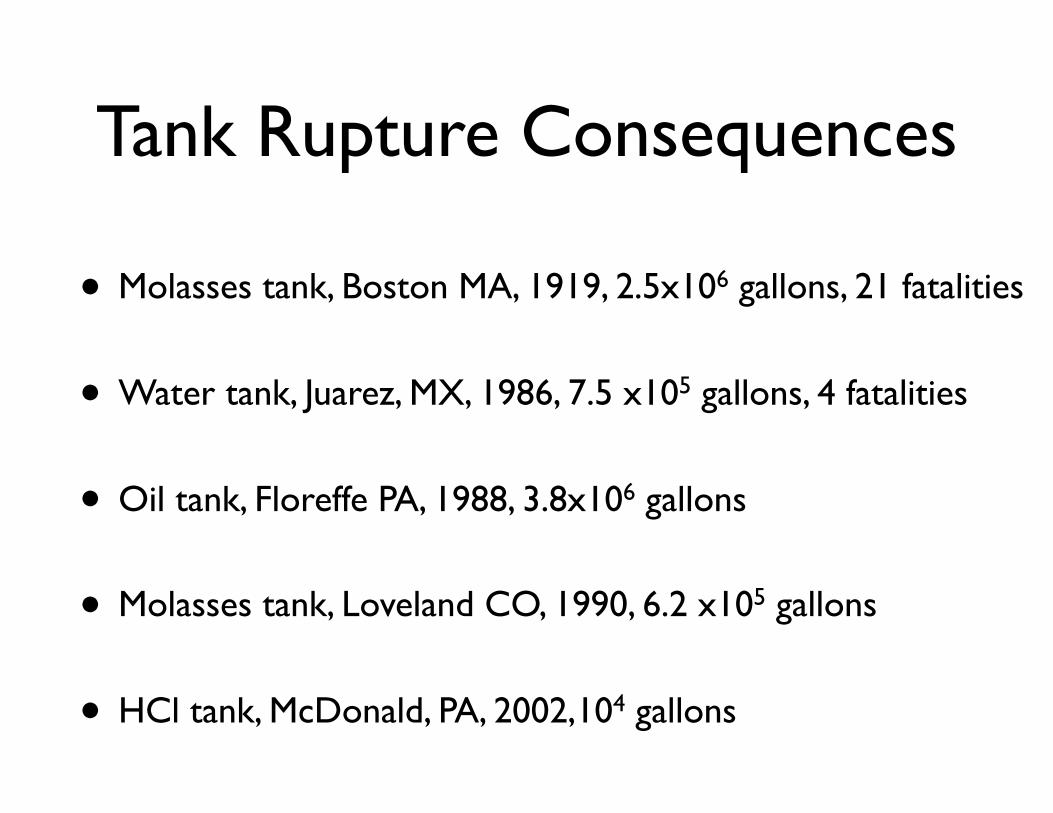
Tank Rupture Consequences
• Molasses tank, Boston MA, 1919, 2.5x10⁶ gallons, 21 fatalities
• Water tank, Juarez, MX, 1986, 7.5 x10⁵ gallons, 4 fatalities
• Oil tank, Floreffe PA, 1988, 3.8x10⁶ gallons
• Molasses tank, Loveland CO, 1990, 6.2 x10⁵ gallons
• HCl tank, McDonald, PA, 2002,104 gallons

Floreffe Aftermath
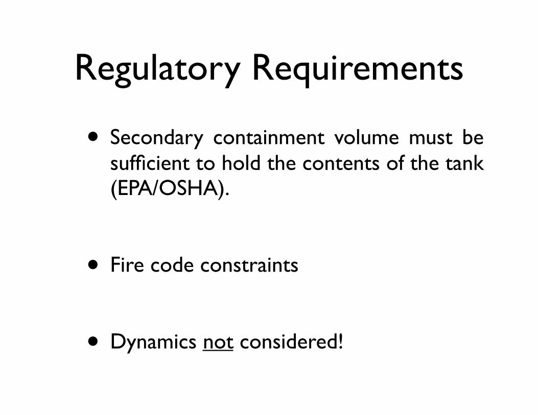
Regulatory Requirements
• Secondary containment volume must be sufficient to hold the contents of the tank (EPA/OSHA).
• Fire code constraints
• Dynamics not considered!

Design Considerations
• Dike height
• Dike diameter
• Dike shape
• Complete tank rupture
• Small hole in tank wall

Rupture Flow Scales
• Height: H ∼ 10 m
• Distance: L ∼ 10 m
• Velocity: (gH)1/2 ∼ 10 m/s
• Time: L/(gH)1/2 ∼ 1 s
• Reynolds number: Re ∼ 108
Initial Condition
H
L

Shallow-Water Theory
• Depth-averaged inviscid equations of motion
• Exact mass balance
• Hydrostatic pressure
• Analogous to compressible gas dynamics
h + ∇•(hu) = 0
u + u•∇u + ∇h = 0
•
• h ⇒u ⇒ ⇒

Shock Conditions
• Multi-valued SWT solutions
• Supplemental jump equations
u+ − λ( )h+ − u− − λ( )h− = 0
u+ − λ( )2 h+ − u− − λ( )2 h− +12(h+ )2 − (h− )2( ) = 0 (-) (+)
⇐ λ

Numerical Pitfalls
• Diffusive Errors
• Dispersive Errors

Computational Methods
• Method of Characteristics
• Explicit Finite-Difference (Lax, FCT, WENO)
• Implicit Finite Element (DG, SUPG)
• Projection Methods (POD)

Method of Characteristics
φ =hu⎧⎨⎩
⎫⎬⎭
⇒ Ai∂φ∂t
+ Bi∂φ∂x
+ψ = 0
Eigenvalue: λ ξiA( ) = ξiB
ξiA( )i ∂φ∂t
+ λ ∂φ∂x
⎧⎨⎩
⎫⎬⎭+ ξiψ = 0
ξiA( )idφdt
+ ξiψ = 0 : dxdt
= λ

Simple Planar WaveWavespeed : c = h
dhdt
± cdudt
= 0 : dxdt
= u ± c
x
t
c = 0u = 0
c = 1u = 0
c =23−
13
x −αt
⎛⎝⎜
⎞⎠⎟
: u = 23+
23
x −αt
⎛⎝⎜
⎞⎠⎟
Splash

Lax FD Method
x
t
i + 1, ji, j i - 1, j
i, j + 1
∂h∂t
+∂q∂x
= 0 : q ≡ uh
⇓
hi, j+1 =12hi−1, j + hi+1, j( ) − Δt
2Δx⎛⎝⎜
⎞⎠⎟qi+1, j − qi−1, j( )

Planar Rupture Splash

Complete Rupture Symmetric Planar Flow
0.0 0.2 0.4 0.6 0.8 1.00.0
0.2
0.4
0.6
0.8
1.0
Wall Position
DikeSplash
Complete Rupture: Planar Flow
a d0.80 0.990.60 0.960.40 0.900.30 0.840.20 0.760.15 0.690.10 0.590.05 0.41

Polar Rupture Splash
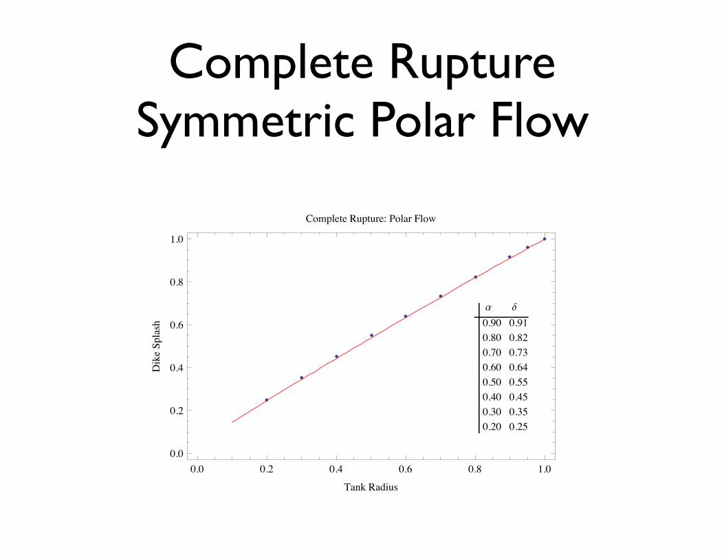
Complete Rupture Symmetric Polar Flow
0.0 0.2 0.4 0.6 0.8 1.00.0
0.2
0.4
0.6
0.8
1.0
Tank Radius
DikeSplash
Complete Rupture: Polar Flow
a d0.90 0.910.80 0.820.70 0.730.60 0.640.50 0.550.40 0.450.30 0.350.20 0.25
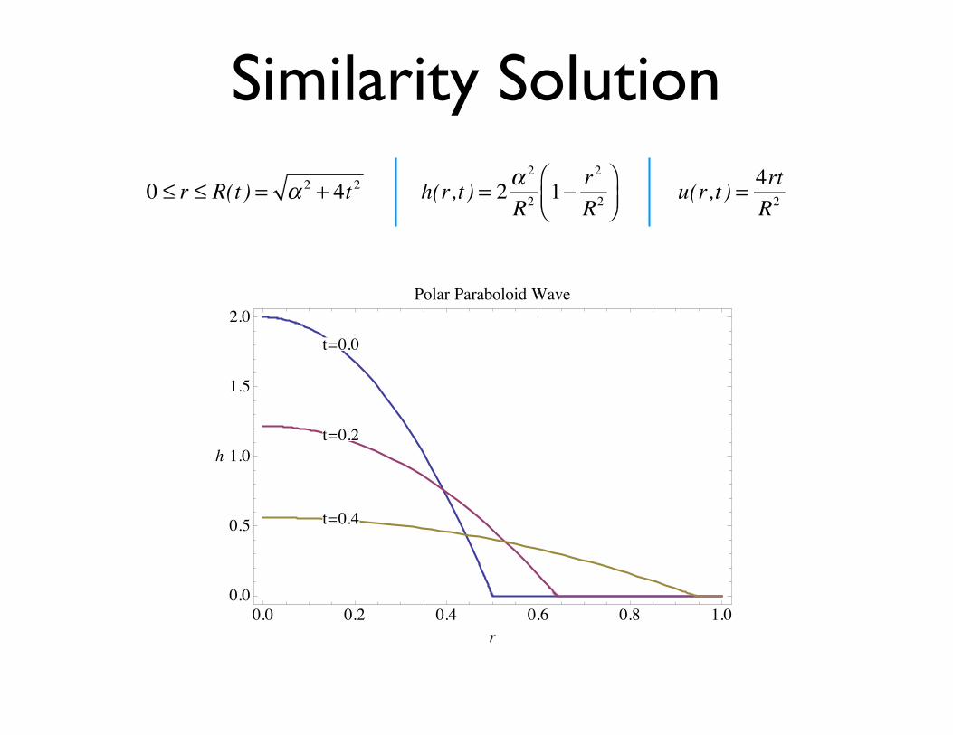
Similarity Solution
0.0 0.2 0.4 0.6 0.8 1.00.0
0.5
1.0
1.5
2.0
r
h
Polar Paraboloid Wave
t=0.0
t=0.2
t=0.4
0 ≤ r ≤ R(t ) = α 2 + 4t 2 h(r,t ) = 2α2
R2 1− r2
R2
⎛⎝⎜
⎞⎠⎟
u(r,t ) = 4rtR2
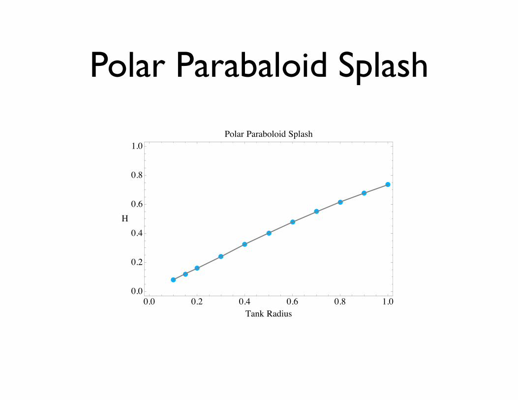
Polar Parabaloid Splash
0.0 0.2 0.4 0.6 0.8 1.00.0
0.2
0.4
0.6
0.8
1.0
Tank Radius
H
Polar Paraboloid Splash

Rupture Flow Experiments
• Greenspan & Young (1978)
(a) planar flow, validated SWT
(b) sloped dikes particularly ineffective
(c) initial splash exceeds tank height
• Greenspan & Johansson (1981)
(a) polar flow
(b) dike shape study
(c) proposed trip rings, deflectors

Summary
• Low (equilibrium) dikes do not contain rupture flow
• Shallow Water Theory can be applied to address:
(a) small hole splash
(b) dike overflow
(c) multiple dike interaction
• Small-scale experiments are representative