NASA Contractor Report 201646

ICASE Report No. 97-5

it ANNIVERSARY

STORAGE ALTERNATIVES FOR LARGE STRUCTURED STATE SPACES

Gianfranco Ciardo j Andrew S. Miner

NASA Contract No. NAS1-19480 January 1997

Institute for Computer Applications in Science and Engineering NASA Langley Research Center Hampton, VA 23681-0001

Operated by Universities Space Research Association

National Aeronautics and Space Administration

Langley Research Center Hampton, Virginia 23681-0001 mW013

Storage alternatives for large structured state spaces*

Gianfranco Ciardo Andrew S. Miner

Dept. of Computer Science

College of William and Mary

Williamsburg, VA 23187-8795, USA

{ciardo,asminer}@cs.wm.edu

Abstract

We consider the problem of storing and searching a large state space obtained from a high- level model such as a queueing network or a Petri net. After reviewing the traditional technique based on a single search tree, we demonstrate how an approach based on multiple levels of search trees offers advantages in both memory and execution complexity, and how solution algorithms based on Kronecker operators greatly benefit from these results. Further execution time improvements are obtained by exploiting the concept of "event locality." We apply our technique to three large parametric models, and give detailed experimental results.

*This research was partially supported by the National Aeronautics and Space Administration under NASA Contract No. NAS1-19480 while the first author was in residence at the Institute for Computer Applications in Science and Engineering (ICASE), NASA Langley Research Center, Hampton, VA 23681- 00091 and by the Center for Advanced Computing and Communication under Contract 96-SC-NSF-1011

1 Introduction

Extremely complex systems are increasingly common. Various types of high-level models are used to describe them, study them, and forecast the effect of possible modifications. Unfortunately, the logical and dynamic analysis of these models is often hampered by the combinatorial explosion of their state spaces, a problem inherent with discrete-state systems. Possible solutions are:

• Use approximate or bounding analysis methods. These are particularly effective when studying the performance or reliability of a system described by a stochastic model (such as a queueing network or a stochastic Petri net).

• Use discrete-event simulation. This does not require the generation and storing of the entire state space. However, it is a Montecarlo method, and hence it can only state that a certain condition is (or is not) encountered with a certain probability. For example, if the simulation runs performed during an experiment don't find a deadlock, we cannot conclude with certainty that the system is deadlock-free.

• Use exact methods that cope with large state spaces. These include the use of bet- ter algorithms and data-structures and of distributed approaches exploiting multiple workstations, plus, of course, the trivial (but expensive) approach of increasing the amount of RAM.

We stress that the above approaches are not mutually exclusive. Indeed, it is quite common to use exact methods in the early stages of a system's design, when studying rough models over a wide range of parameter combinations, and then focus on more detailed models using approximate methods or simulation. Indeed, many approximate decomposition approaches use exact methods at the submodel level, thus introducing errors only when exchanging or combining (exact) results from different submodels. Then, the ability of applying exact methods to larger models will normally result in better approximations: it is likely that the study of a large model decomposed into four medium-size submodels, each solved with exact methods, will be more accurate than that of the same model decomposed into ten small-size submodels.

The first problem when applying exact methods is the generation and storage of the state space. For performance or reliability analysis, the model is then used to generate a stochastic process, often a continuous-time Markov chain (CTMC), which is solved numerically for steady-state or transient measures. The state space itself can be of interest since it can be used to answer questions such as existence of deadlocks and livelocks or liveness.

In this paper, we focus on techniques to store and search the state space. However, while we do not discuss the solution of the stochastic process explicitly, our results apply not only to the "logical" analysis of the model, but even more so to its "stochastic analysis" (indeed, this was our initial motivation). This is particularly true given the recent developments on the solution of complex Markov models using Kronecker operators [2, 3, 9, 12, 13, 15, 17] which do not require the storage of the infinitesimal generator of the CTMC explicitly. In

this case, the storage bottleneck is indeed due to the state space and the probability vectors

allocated when computing the numerical solution. Sections 2, 3, and 4 define the type of high-level formalisms we use, discuss the reachability

set and its storage, and motivate the decomposition of a model into submodels, respectively. Our main contributions are in Sections 5 and 6, where we introduce a multilevel data struc- ture and show how it can be used to save both memory and execution time when building the reachability set. Section 7 further explores storing and searching the reachability set

after it has been built. Finally, Section 8 contains our final remarks.

2 High-level model description

We implemented our techniques in SMART [7], using the GSPN formalism [1, 5]. However, these techniques can be applied to any model expressed in a "high-level formalism" which

defines:

• The "potential set", Ü. This is a discrete set, assumed finite, to which the states of

the model must belong1.

• A finite set of possible events, £.

• An initial state, i° G U.

• A boolean function defining whether an event is active (can occur) in a state, Active :

£ x Ü -*• {True, False}.

• A function defining the effect of the occurrence of an active event on a state: New :

£xii->n. Fig. 1 and 2 show the two GSPNs used throughout this paper to illustrate the effect of

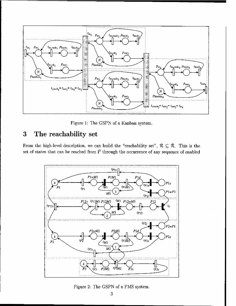
our techniques (ignore for the moment the dashed boxes). The first GSPN models a kanban systems, from [9, 17]. It is composed of four instances of essentially the same sub-GSPN. The synchronizing transitions tsynchl and tsynch2 can be either both timed or both immediate, we indicate the two resulting models as kanban-timed and kanban-immediate. The second GSPN models a flexible manufacturing system, from [10], except that the cardinality of all arcs is constant, unlike the original model (this does not affect the number of reachable markings). We indicate this model as FMS. We do not describe these models in more detail, the interested reader is referred to the original publications where they appeared.

*A point about notation: we denote sets by upper case calligraphic letters. Lower and upper case bold letters denote vector and matrices, respectively. r,(A) is the number of nonzero entries in a matrix A; A* j is the entry in row i and column j of A; Ax,y is the submatrix of A corresponding to the set of rows X and

the set of columns y.

• Pkanban? tsynchf ^om-f ^out-f Un^

Figure 1: The GSPN of a Kanban system.

3 The reachability set

From the high-level description, we can build the "reachability set", % C TZ. This is the set of states that can be reached from i° through the occurrence of any sequence of enabled

■'P\2:

fPlj

P\wM\ PIMl

tpl tpiMl h Pl2s tP12M3P12M3 *M3 p\2wM3

PlwMl P2M2 PU

Figure 2: The GSPN of a FMS system.

3

BuildRS{\n: Events, Active, New; out: 11); I -ft «_ 0; /* Ji: states explored so far */

2. u «- {i0}; /*U: states found but not yet explored */

3. while U ± 0 do 4. i 4- ChooseRemove(U);

5. ?e^^U{i}; 6. for each e G £ s.t. Active{e, i) = True do

7. j •<- JVeu<e, i); 8. SearchInsert(j,1l\JU,U);

Figure 3: Procedure BuildRS

events. Formally, U is the smallest subset of Ü satisfying:

• i° € U, and

• i G n A 3e € 5,4dwe(e, i) = True A i' = New{e, i) =M' G H.

While a high-level model usually specifies other information as well (the stochastic timing of the events, the measures that should be computed when solving the model, etc.), the above description is sufficient for now, and it is not tied to any particular formalism.

Tl can be generated using the state-space exploration procedure BuildRS shown in Fig. 3, which terminates if 11 is finite. This is a search of the graph implicitly defined by the model. Function ChooseRemove chooses an element from its argument (a set of states), removes it, and returns it. Procedure Searchlnsert searches the first argument (a state), in the second argument (a set of states) and, if not found, it inserts the state in its third argument (also

a set of states). The "reachability graph", (K,A), has as nodes the reachable states, and an arc from i

to j iff there is an event e such that Active{e, i) = True and New{e, i) = j. Depending on the type of analysis, the arc might be labelled with e; this might result in a multigraph, if multiple events can cause the same change of state. While we focus on U alone, the size of

A affects the complexity of BuildRS. A total order can be defined over the elements of 11: i < j iff i precedes j in lexical order.

We can then define a function Compare : {£ x %) -» {-1,0,1} returning -1 if the first argument precedes the second one, 1 if it follows it, and 0 if the two arguments are identical. This order allows the efficient search and insertion of a state during BuildRS. Once 11 has been built, we can define a bijection * : K -► {0,..., \R\ - 1}, such that tf (i) < *(j) iff

i < j. Common techniques to store and search the sets K and U include hashing and search

trees. Hashing would work reasonably well if we had a good bound on the final size of the reachability set K, but this is not usually the case. We prefer search trees: when kept

balanced, they have more predictable behavior than hashing.

We consider two alternatives, both based on binary search trees: splay trees [11] and AVL trees [14]. The execution complexity2 of BuildRS when using either method is

O (\K\ ■ \£\ • CActive + \A\ ■ (CNew + log 1-72-1 • Compare)) ,

where Cx is the (average) cost to a call to procedure x. For AVL trees, the storage complexity, expressed in bits, is

O (\1Z\ ■ (Bgtate + ^Bpointer + 2)) ,

where Bstate is the (average) number of bits to store a state, Bpointer is the number of bits for a pointer. The additional two bits are used to store the node balance information. For splay trees, the complexity is the same, except for the two-bit balance, which is not required.

Regarding the use of binary search trees in BuildRS, we have another choice to make. We can use a single tree to store 1ZUU in BuildRS as shown in Fig. 4(a,b,c), or two separate trees, as in Fig. 4(d). Using a single tree has some advantages:

• No deletion, possibly requiring a rebalancing, is needed when moving a state from U

toTl.

• Procedure Searchlnsert needs to perform a single search with log(|7lUW|) comparisons, instead of two searches in the two trees for 11 and U, which overall require more comparisons (up to twice as many), since

log \n\ + log \u\ = \og(\n\ ■ \u\) > iog(\n\ + \u\) = \og(\n u u\)

(of course, we mean "the current 1Z and W in the above expressions).

However, it also has disadvantages. As explored and unexplored states are stored together in a single tree, there must be a way to identify and access the nodes of U. We can accomplish this by:

• Maintaining a separate linked list pointing to the unexplored states. This requires an additional 0{2\U\ ■ Bpointer) bits, as shown in Fig. 4(a).

• Storing an additional pointer in each tree node, pointing to the next unexplored state. This requires an additional 0{\H\ • Bpointer) bits, as shown in Fig. 4(b).

• Storing the markings in a dynamic array structure. In this case, the nodes of the tree contain indices to the array of markings, instead of the markings themselves. If markings are added to the array in the order they are discovered, 1Z occupies the beginning of the array, while U occupies the end. This requires an additional 0(\H\ • Bindex) bits, where Bindex is the number of bits required to index the array of markings, as shown in Fig. 4(c)

The size of 1Z for our three models is shown in Table 1, as a function of N. Since the models are GSPNs, they give rise to "vanishing markings", that is, markings enabling only immediate transitions, in which the sojourn time is zero. In all our experiments, these markings are eliminated "on the fly" [8], so that all our figures regarding H reflect only the "tangible" reachable markings.

2We leave known constants inside the big-0 notation to stress that they do make a difference in practice,

even if they are formally redundant.

¥ rS—i—i < c > < k >

<b> < f > • < i > < 1 >

< a > < e > < g > -.•■ < j > -. < m

KAT < dl>

(a)

>

(b)

I

< i

\-\ < c > •:-.. <|k >

<b> : < f > •: < i > •: <

»>•: <e> :<g> : <j>

I > :

\ .. : < m >

Tj taaaBB^: • ; •:—►: •; •:—►: •; •:—►: •'. •:—►• • - • '■—^: •' ^ < = > 4— RuU i L

' n/ta" < = > f <\= > i < = > < = >

> *<=r>i< = >« < = >i< _U / L_J l_l %L_J LJ , l_l LJ ,L_L

m \ ] ! --▼ —i T*-- *h \

<|g > < k >

<b|> <e|> <j> <m> < =

' *-!" 1

1 4

'l 1 X \ \

' »b I .-•-.-* g | .* *■ k |

A — S

< c > < 1 >

1 \ / <|a|> <|d > < i >

<

>

—L-J - - \. A*-

»«■ * ' - - -

Figure 4: Four simple storage schemes for 11 and W.

iV 7£ for kanban-timed \R\ for kanban-immediate 1-72-1 for FMS

1 160 152 54

2 4,600 3,816 810

3 58,400 41,000 6,520

4 454,475 268,475 35,910

5 2,546,432 1,270,962 152,712

6 11,261,376 4,785,536 537,768

7 - - 1,639,440

Table 1: Reachability set size for the three models, as a function of N.

4 Structured state spaces

We now assume that K can be expressed as the Cartesian product of K "local" state spaces: 1Z = n0x---x KK-\ and that Kk is simply {0,... nk -1}, although nk might not be known in advance. Hence, a (global) state is a vector i e {0,... n0 -1} x • • • x {0,... nK-x -1}- For example, if the high-level model is a single-class queuing network, ik could be the number

of customers in queue k. However, a realistic model can easily have dozens of queues; so it might be more efficient to partition the queues into K sets, and let i^ be the number of possible combinations of customers into the queues of partition k. An analogous discussion applies to stochastic Petri nets (SPNs), and even to more complex models, as long as they have a finite state space.

Such a structured model definition is essential to the Kronecker approach for the spec- ification and solution of complex Markov models recently proposed by various authors [2, 3, 12, 13, 15]. The main idea is that the infinitesimal generator Q of a large model composed of K submodels can be described as (a submatrix of) a sum of Kronecker prod- ucts of K smaller matrices, each related to a different submodel. Without going into further details, we simply list a few key features of this approach, which prompted much of our work.

• The potential set 71 is the Cartesian product of K local state spaces, one for each submodel. Our lexical order can be applied just as well to 7t, hence we can define a bijection \P : 71 —> {0,..., \7l\ — 1}, analogous to \I>. Indeed, ^ has a fundamental advantage over \P: its value equals its argument interpreted as a mixed base integer,

K-l

*(i) = (... ((io)ni + ii)n2 • • >K-i + ijr-i = £ i* • w*+i\ k=0

K-l

£ fc=0

where nf = \[3k=ink.

• The reachability set 71 may coincide with K, but it is more likely to be much smaller, since many combinations of local states might not occur.

• Numerical solutions compute the steady-state probabilities of each state using either a vector Or of size \Ü\ or a vector TV of size \R\. In the former case, the probability of state i G 71 is stored in "fry,*, while the entries of 7r corresponding to unreachable states are not used, they are initially set to zero and never modified [12]. In the latter case, the same probability is stored in 7r^(i) [13]. We prefer this second approach because it requires potentially much less memory. However, as described by Kemper, its complexity has an additional 0(log \7l\) multiplicative factor, since, for each reachable state i G 7t and for each possible transition from i to j, the index \f(j) of j in iz must be computed using a binary search.

• Any steady-state or transient solution method that avoids storage and execution com- plexity of order \R\ must iterate over the elements of 71 in some order. The lexical order is acceptable, especially for methods such as Power, Jacobi, or Uniformization, which are not affected by the order in which the variables are considered. To clarify the relevant complexity issues, we show procedure VectMatrMultiply in Fig. 5, to perform the assignment

y <- y + x • (A0 <g> A1 ® • • • ® AK~1) ^ J \ ) 11,11

where Ak is a matrix of order nk and the subscript "7£, TV indicates the submatrix of the Kronecker product corresponding to the reachable states only. This is the main operation needed when solving for the steady state or transient probabilities for any

VectMatrMidtiplyQn: x, K, K, A0, A1,..., A*-1; inout: y) 1. for each i € 1Z do

2. I <- *(i); 3. for each j0 s.t. A?oJo > 0 do

4. ao 4- A?ojo; 5. for each ji s.t. Aj^ > 0 do

6. oi <- a0 • Ajls ui1

7. for each j^_i s.t. 'A£_J Jjr-1 > 0 do

8. aK_x <- aK-2 • AK_1 'K-UK-l

iK-lJK-1'

9. J <- *(j); 10. if J ^ null then

11. yj «-y.r + x/-ajr_i;

Figure 5: Procedure to multiply a vector by a submatrix of a Kronecker product.

approach based on Kronecker algebra over data structures of size 0(|7l|). For example, with the Power method, x is the old iterate for TT while y accumulates what will be the new iterate. We stress that the procedure VectMatrMultiply relies heavily on the extreme sparsity of the matrices involved (assumed to be stored in sparse row-wise format), while algorithms such as those proposed by Plateau and Stewart [16] are

more appropriate for full matrices.

In the case of superposed GSPNs [12], the test J # null of statement 10 is always satisfied, hence, it should be apparent that procedure VectMatrMultiply considers all and only the nonzero entries in the submatrix An,n of A. The overall complexity is then affected by the log \TZ\ overhead to compute the index J of j in 1Z, in statement 9, within the innermost for-loop:

0(v(An,n)-\og\Tl\).

Hence, two main limitations in [13] prevent the application of this approach to truly enormous problems. First, the storage of the state space 11 and of the iteration vectors, also of size \R\ might require excessive memory. Second, from an execution time standpoint, the log | K | factor represents an additional complexity with respect to the traditional approach

where the iteration matrix is stored explicitly. In the next sections, we show how the memory requirements can be reduced, while

improving the execution complexity at the same time.

5 A multilevel search tree to store TZ

We extend work by Chiola, who defined a multilevel technique to store the reachable markings of a SPN [4]. Since the state, or marking, of a SPN with K places can be represented as a

8

\

\

a:001

b:002

c:011

d:102

e:004

/" 1 • —► a

—► b

—► e

2 • 0 •

0 • 4 • 1 •

1 • 1 • —► c

0 •

2 • —► d

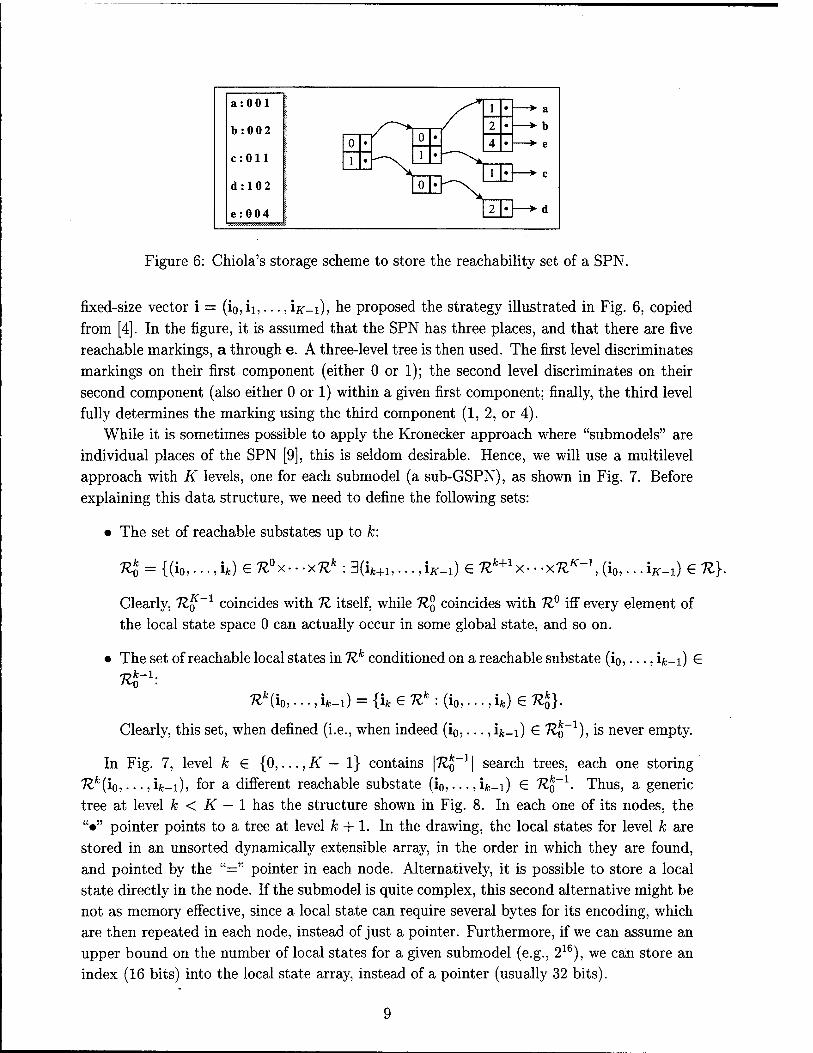
Figure 6: Chiola's storage scheme to store the reachability set of a SPN.

fixed-size vector i = (i0, ii,..., ijr-i), he proposed the strategy illustrated in Fig. 6, copied from [4]. In the figure, it is assumed that the SPN has three places, and that there are five reachable markings, a through e. A three-level tree is then used. The first level discriminates markings on their first component (either 0 or 1); the second level discriminates on their second component (also either 0 or 1) within a given first component; finally, the third level fully determines the marking using the third component (1, 2, or 4).

While it is sometimes possible to apply the Kronecker approach where "submodels" are individual places of the SPN [9], this is seldom desirable. Hence, we will use a multilevel approach with K levels, one for each submodel (a sub-GSPN), as shown in Fig. 7. Before explaining this data structure, we need to define the following sets:

• The set of reachable substates up to A;:

ft {(i0,...,ifc) G n°x-■ -xnk: 3(ifc+1,...,!*_!) G nk+1x-• -xnK-\ (i0,...i*-i) G ft}.

Clearly, ftjf * coincides with ft itself, while ftp coincides with ft0 iff every element of the local state space 0 can actually occur in some global state, and so on.

The set of reachable local states in ftfe conditioned on a reachable substate (io,..., ifc_i) G

ftfe(i0,..., ifc_0 = {ife G ftfc : (i0,..., ifc) G ft*}. nt1-.

Clearly, this set, when defined (i.e., when indeed (io,..., ifc_i) G TZQ ), is never empty.

In Fig. 7, level k G {0,...,K - 1} contains [RJQ | search trees, each one storing ftfe(io,..., ifc-i), for a different reachable substate (io,..., ifc_i) G K Thus, a generic tree at level k < K — 1 has the structure shown in Fig. 8. In each one of its nodes, the "•" pointer points to a tree at level k + 1. In the drawing, the local states for level k are stored in an unsorted dynamically extensible array, in the order in which they are found, and pointed by the "=" pointer in each node. Alternatively, it is possible to store a local state directly in the node. If the submodel is quite complex, this second alternative might be not as memory effective, since a local state can require several bytes for its encoding, which are then repeated in each node, instead of just a pointer. Furthermore, if we can assume an upper bound on the number of local states for a given submodel (e.g., 216), we can store an index (16 bits) into the local state array, instead of a pointer (usually 32 bits).

9

Level 0

Level 1

Level K-\

Figure 7: A multilevel storage scheme for 11.

Rginv.-^-i) f • < = >

• < = >

»•:.-'

= >

• < = > • < = >

I

s -'----.- '

R^'an.-^i.a,) I

Local states for level k

> a4:

I*:.

b«.: I

ek:

c*:

Rt+1(in,-Jt.i,ct)J R^1(in,-,i.-iet)^I :

R*:'(in,,.,iM:b*) j l^^:::A',g^ IJ^fekM

Figure 8: A tree at level k < K -1, pointing to trees at level k + 1.

The total number of nodes used for trees at level k equals the number of reachable substates up to that level, |ft§|, hence the total number of tree nodes for our multilevel data

structure is

E 1*51 > K_1l = 1*1 k-0

where the last expression is the number of nodes required in the standard single-level ap-

proach of Fig. 4. Two observations are in order:

10

• First, the total number of nodes at levels 0 through K — 2 is a small fraction of the nodes at level K — 1, that is, of |7£|, provided the trees at the last level, K — 1, are not "too small". This is ensured by an appropriate partitioning of a large model into submodels. In other words, only the memory used by the nodes of the trees at the last level really matters.

• Second, the nodes of the trees at the last level do not require a pointer to a tree at a lower level, hence each node requires only three pointers (96 bits). Again, if we can assume a bound on the number of local states for the last submodel, |7£K_1| < 26, we can in principle implement dynamic data structures that require only 36 bits per node, plus some overhead to implement dynamic arrays. Given a model, there is usually some freedom in choosing the number of submodels, that is, the number of levels K. We might then be able to define the last submodel in such a way that is has at most 28 local states, resulting in only slightly more than 3|7£| bytes to store the entire reachability set. When this is not the case, the next easily implementable step, 216, is normally more than enough. Even in this case, the total memory requirements are still much better than with a single-level implementation.

We stress that, while this discussion about using 8 or 16 bit indices seems to be excessively implementation-dependent, it is not. Only through the multilevel approach it is possible to exploit the small size of each local space. In the single-level approach, instead, the total number of states that can be indexed (pointed by a pointer) is \R\, a number which can be easily be 107, and possibly more. In this case, we are forced to use 32-bit pointers, and we can even foresee a point in the not-so-distant future where even these pointers will be insufficient, while the multilevel approach can be implemented using 8 or 16 bit indices at the last level regardless of the size of the reachability set, as long as KK~l is not too large.

Just as with a single search tree, we can implement our multilevel scheme using splay or AVL trees. However, the choice between storing K and U separately or as a single set has subtler implications. If we choose to store them as a single set, distinguishing between explored and unexplored states or, more precisely, being able to access the unexplored states only, still requires one of the approaches discussed for the single-level case (Fig. 4). Since only local states are stored for each level, without repetition, we can no longer use the state array approach of Fig. 4(c). The other two methods, which involve maintaining a list of unexplored states, would only allow us to access nodes in trees at level K — 1, which are meaningless if we do not know the entire path from level 0. In other words, we would only know the last component of each unexplored state, but not the first K — 1 components. To obtain all the components, we must add a backward pointer from each node (conceptually, from each tree, since all the nodes in a given tree have the same previous components) to a node in the previous level, and so on. This additional memory overhead is substantial.

With the single-level approach, then, we store TZUU in a single tree, using the state array described in Fig. 4(c). With the multilevel approach, instead, we store % and U separately. In this second case, states are truly deleted from U. However, we are free to remove states in any order we choose. When using AVL trees, we use the balance information to choose, at each level, a state in a leaf of the tree in such a way that no rebalancing is ever required.

11

Memory (kanban-timed) Memory (kanban-immediate) oe-i-u/

5e+07

4e+07

i i i

Single Multi

i

•+■■

l

3e+07 / ■£

2e+07 •' -

le+07 /%

-

0 W— *' i i

oe-i-ur

2.5e+07

i l l i

Single -O- Multi ■+• ■

i

2e+07 - / -

1.5e+07 - / +

le+07 -

5e+06

0 ■0—

/A-

<1>—-^& \ i

4e+07

3.5e+07

3e+07

2.5e+07

2e+07

1.5e+07

le+07

5e+06

0

Memory (FMS)

Single Multi

-0- /- ■+■- /

- / ^

- i i

d> <s> fr-4 ? ■ T i i

3 3 iV

12 3 4 5 6

Figure 9: Memory usage (bytes) for the single and multilevel approaches.

Fig. 9 shows the number of bytes used to store 11 and U, separately, for our three models, using the single vs. the multilevel approach. The dashed boxes in Fig. 1 and 2 indicate how the models have been decomposed into submodels, in all cases K = 4.

The multilevel approach is clearly preferable, especially for large models. Indeed, we could not generate the state space using the single-level approach for N - 6 for the kanban- timed model, while we could using the multilevel approach (all our experiments where run on a Sun-clone with a 55 MhZ HyperSparc processor and 128 Mbyte of RAM, without making

use of virtual memory).

6 Execution time

Several factors need to be considered when studying the impact of our approach on the execution time. First, we explored possible differences due to using splay trees vs. AVL trees. Fig. 10 shows that no method is clearly better and that, in most cases, the differences are minor in comparison to the effect due to the choice of a single vs. a multilevel data

structure. We then focussed on this second factor, using AVL trees exclusively. The advantages of

the multilevel approach are:

• Consider first the case when BuildRSseaxch.es for a state i not yet in the current U (the same discussion holds for U). With a single-level tree, the search will stop only after reaching a leaf, hence 0(log \7L\) comparisons are always performed. In the multilevel approach, instead, the search stops as soon as the substate (ii,..., ifc) is not reachable, for some k <K-1. If all the trees at a given level are of similar size, this will require at most 0(log|ft§|) comparisons. In practice, the situation is even more favorable, because, for any level I < k, the tree searched, which stores Hl{U,... ,ij-i), contains

12

Time (kanban-timed) zUUU

0000

8000

i i i i i

- Single AVL S- £ Single Splay ■+■ • /

Multi AVL -B- / " Multi Splay -X-- f

6000 -

4000

/ "

2000

0 m es -flr i L

7000

6000

5000

4000

3000

2000

1000

0

Time (kanban-immediate)

- Single AVL -0- Single Splay ■+■

Multi AVL S- Multi Splay -X--

3 N

9000 Time (FMS)

i i i i i i

8000

7000

6000

- Single AVL ^- Single Splay •+■ -

" Multi AVL -Q- Multi Splay -X- -

fr

5000 - // ~

4000 i / -

3000 J -

2000 m -

1000

0 fg—gg—6g -flri—L i

2 3 4 5 N

6 7

Figure 10: Execution times (seconds) for the AVL and splay trees.

the substate ij we are looking for, so the jump from level I to level I + 1 might occur before reaching a leaf.

• If i is already in TZ, instead, the search on the single-level tree will sometimes find i before reaching a leaf, but this is true also at each level of the multilevel approach, just as in the previous case, for the levels I < k.

• Perhaps even more important, regardless of whether i is already in the tree or not, is the complexity of each comparison. With the multilevel approach, only substates are compared, and these are normally small data structures. For GSPNs, this could be an array of 8 or 16 bit integers, one for each place in the sub-GSPN (memory usage is not an issue, since each local state for level k is stored only once). On the other hand, with the single-level approach, entire states are compared. If the states are stored as arrays, the comparison can stop as soon as one component differs in the two arrays. However, as the search progresses down the tree, we compare states that are increasingly close in lexical order, hence likely to have the same first few components; this implies that comparisons further away from the root tend to be more expensive. Furthermore, storing states as full arrays is seldom advisable. For example, in SMART, a sophisticated packing is used, on a state-by-state base, to reduce the memory requirements. In this case, the state in the node needs to be "unpacked" before comparing it with i, thus effectively examining every component of the state.

13

Section 7 further investigates the complexity of searching a state, reachable or not, after the entire reachability set has been explored.

6.1 Exploiting event locality

Our multilevel search tree has an additional advantage which can be exploited to further speed up execution. To illustrate the technique, we define two functions:

• LocalSet(k, Ik-i), which, given a submodel index k, 0 < k < K, and a pointer Ik-i to a reachable substate (i0,..., ifc_i) € Til'1, returns a pointer to the tree containing the

set ft*(i0,...,ik_i).

• LocalIndex(k, Ik-i, ifc), which, given a submodel index k, 0 < k < K, a pointer Ik-\ to a a reachable substate (i0, • • •, h-i) G 1Zk

0~\ and a local state index ife G Kk, returns the pointer Ik to substate (i0,..., ifc), if reachable, null otherwise.

Given our data structure, "a pointer Ik to a reachable substate (i0,..., ifc) € fto" points to the node corresponding to the local state ifc in the tree containing the set 7lfc(i0,..., ifc_i).

To find whether state i is in (the current) 11, we can then use a sequence of K function

calls

LocalIndex(K-l, LocalIndex(K - 2,... LocalIndex(l, Locallndex(0, null, i0), ii),.. AK-2), ijr-i)-

IK-2

The overall cost of these K calls is exactly what we just discussed when comparing the single and multilevel approaches. However, if i is reachable and we now wanted to find the index of a state i' differing from i only in its last position, we could do so with a single

call LocalIndex{K - 1, IK-2, ijc-i)» provided we have saved the value IK_2, the index of the reachable substate (i0, ■ • •, ijf-2). A similar argument applies to other values of k. Only for k = 0 we need to perform an entirely new search.

We can then exploit this "locality" by considering the possible effects of the events on the state. Given K = 71° x • • • KK~l, we can partition £ into £°,..., £K~\ such that

ee5*<=» (Vi G n, Active{e, i) = True A j = New(e, i) =» VJ, 0 <l < fc, ij = jj) ,

that is, events in £k can only change local states k or higher. For example, for GSPNs, this is achieved by assigning to £k all the transitions whose enabling and firing effect on the state depends only on places in sub-GSPN k, and possibly in sub-GSPNs k + 1 through K - 1, but not in sub-GSPNs 1 through k-\. This can be easily accomplished through an automatic inspection even in the presence of guards and inhibitor and variable cardinality arcs (although in this case the partition might be overly conservative, that is, it might assign a transition to a level k when it could have been assigned to a level I > k).

When exploring state i, in procedure BuildRS, we remove i from U and insert it into 11, obtaining, as a byproduct, a sequence of pointers /_x = null, I0,..., IK-2, to the reachable substates (i0),.. •, (io, • • • ,1^-2)• Then, we can examine the events in £ in any order. As soon as we find an enabled event e G £k, we generate i' = New(e, i), and we are guaranteed

14

Time (kanban-timed) 12000 n 1—

Time (kanban-immediate)

10000

8000 \-

6000

4000

2000

0

Single -^- Multi +• - Local -B—

7000

6000

5000

4000

3000

2000

1000

0

Single -O- Multi + - Local -B—

9000 Time (FMS)

l 1 i i I I

8000

7000

Single <$- Multi + - Local -Ö— PL

6000 m

5000 7- 4000 / -

3000 -

2000 -

1000 -

0 cr, fJ3^\ | i

1 2 3 4 5 6 N

7

Figure 11: Execution times (seconds) for the single and multilevel approach.

that its components 0 through k — 1 are identical to those of i. Hence, we can search for it starting at h-i, that is, we only need to perform the K — k calls

LocalIndex(K — 1,... LocalIndex(k + 1, LocalIndex(k, h-i, ifc), ijt+i),..., i^-i)-

The savings due to these accelerated searches depend on the particular model and the parti- tion chosen for it. We show the results for our three models in Fig. 11. In this case, savings of 20% execution time or more are achieved. Except for the need to specify a partition, which needs to be done anyway to use our multilevel approach, the technique is completely automatic, and has no additional memory requirements.

6.2 Application to solutions based on Kronecker operators

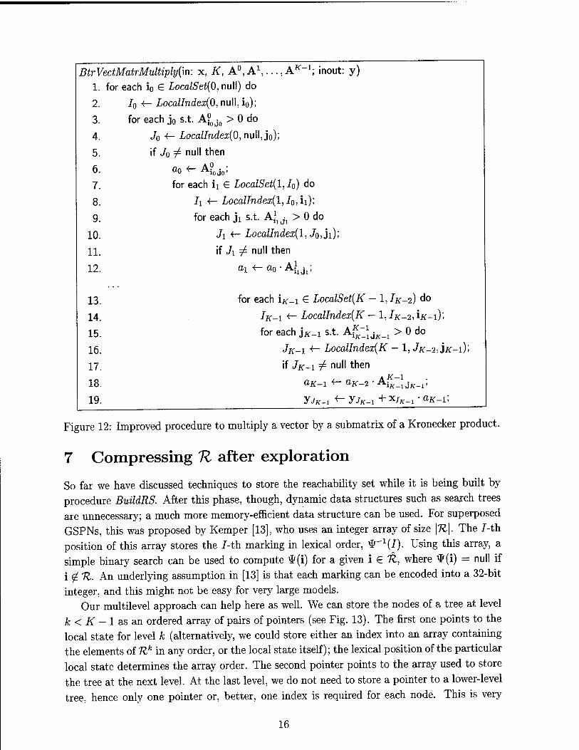
We can also apply our multilevel approach and the principle of locality just introduced to speed up procedure VectMatrMultiply, described in Section 4. An improved version, BtrVectMatrMultiply of the same procedure is shown in Fig. 12. Its complexity is

0(r)({A°)n°,Tio) ■ logn0 + ^((A0 <g> A1)^^) • lognx

+ • • • rj{{A° ® • • • ® AK-l)nK-inK-2xnK^) ■ logrc^x)

Indeed, the term "log?V for the searches at level k is an upper bound, since the size of the tree searched by Locallndex is smaller than n\. if there are any unreachable states; the

"average" size of a tree at level k is (T^ol/I^o-1! ^ nk-

15

BtrVectMatrMultiply{\n: x, K, A0,A1,...,A* 1; inout: y) 1. for each i0 E LocalSet(0, null) do

2. 70 «- LocalIndex(0, null,i0);

3. for each j0 s.t. A?oJo > 0 do

4. Jo <- LocalIndex(0, null, j0);

5. if Jo ¥" nul1 tnen

6- Go <- A?oJo;

7. for each ii € LocalSet(l, Jo) do

8. ii <- Joca/Jnde:c(l, J0,ii);

9. for each jx s.t. A-^ > 0 do

10. Ji <- LocalIndex(l, Jo,ji);

11. if Ji ^ null then

12. ai «-ao-Ajljh;

13. for each \K-\ € LocalSet(K - 1,1^-2) do

14. /K-I «- LocalIndex(K — 1,IK-2,^K-I)',

15. for each j^-i s.t. A?^^ > 0 do

16. J^_x •<- LocalIndex(K - 1, J/r-2, jir-i);

17. if JK-i # null then

18. O-K-l <~ ÖÄ--2 • AKjjr_i:

19. yjjf-i ^ yjjr-i + X'K-I • G^-l;

Figure 12: Improved procedure to multiply a vector by a submatrix of a Kronecker product.

7 Compressing 1Z after exploration

So far we have discussed techniques to store the reachability set while it is being built by procedure BuildRS. After this phase, though, dynamic data structures such as search trees are unnecessary; a much more memory-efficient data structure can be used. For superposed GSPNs, this was proposed by Kemper [13], who uses an integer array of size \K\. The I-th. position of this array stores the J-th marking in lexical order, \&-1(i"). Using this array, a simple binary search can be used to compute *(i) for a given i € 7t, where *(i) = null if i 0 H. An underlying assumption in [13] is that each marking can be encoded into a 32-bit integer, and this might not be easy for very large models.

Our multilevel approach can help here as well. We can store the nodes of a tree at level k < K - 1 as an ordered array of pairs of pointers (see Fig. 13). The first one points to the local state for level k (alternatively, we could store either an index into an array containing the elements of %k in any order, or the local state itself); the lexical position of the particular local state determines the array order. The second pointer points to the array used to store the tree at the next level. At the last level, we do not need to store a pointer to a lower-level tree, hence only one pointer or, better, one index is required for each node. This is very

16

f TL \ft1 \^ *ttt Pointer to next level

\ | • • •

>.

Local state index 1 \

I • • • \ -^ox-:.:""* ■' i -'»""■>■■"»■■"

R° R'Cao) • • •

|R00! IR-I

i |

R'(«o) • • •

• • •

RJC-1(a0,..-,aJf.2) • • • R^(xo,...,zK.2)

|R*J|

Figure 13: Multilevel storage after the reachability set has been built.

desirable, since, as discussed before, only the last level has a major effect on the memory requirements. Using 8 or 16 bit indices, we can then store 11 using only slightly more than \TZ\ or 2\1Z\ bytes, respectively.

The execution time required to transform our tree-based multilevel data structure into the array-based one is negligible, around 1/1000 of the time used by BuildRS. Hence, this transformation is always advisable if searches are to be performed on TZ. This is the case, for example, when computing \?(i) for some i G ft, one of the essential operations in the Kronecker approach we discussed. To further investigate the impact of our multilevel data structure, we computed the expected time required to search for a reachable state i e % (i.e., to compute \I>(i) when i € 11), and for a non-reachable state (i.e., to compute \I>(i) when it is null) in the kanban-timed model. Fig. 14 shows the results for the single vs. the multilevel approach. The dramatic difference in the slope of the curves for the single and multilevel approaches further confirms that our results will greatly improve the efficiency of solution methods based on Kronecker operators.

Also, note how the curves for i e K and i ^ 1Z intersect, in both cases. We generated unreachable states by determining the bound bp on the number of tokens in each place p, then randomly choosing a number np of tokens between 0 and bp for p, independently of the other places. The resulting marking was (almost) always unreachable. For small reachability sets, searching for a reachable state is faster than searching an unreachable state, because we can sometimes stop the search before reaching a leaf. However, as the state space grows, it is increasingly likely that, when searching for an unreachable state, the comparison between two states (or substates, for the multilevel approach) stops after comparing just a few places. Clearly, this effect more than offsets the need to explore up to a leaf for the single-level approach (in the multilevel approach, an additional advantage is that, for an unreachable state, the search might stop at a level k < K — 1).

8 Conclusion

We have presented a detailed analysis of a multilevel data structure for storing and searching the large set of states reachable in some high-level model. Memory usage, which is normally

17

Search time for a single state after compression (kanban-timed) 450

400

350

300

250

200

150'

100

Single i g U ■&- Single i € 11 •+■ - Multi i £ TZ -B- Multi i € ft -X- -

Figure 14: Expected search times (microseconds) for the single and multilevel approach.

the main concern, is greatly reduced. At the same time, this reduction is achieved not at the expense of, but in conjunction with, execution efficiency.

18

A further technique based on event locality achieves an additional reduction in the exe- cution time, with no additional memory cost.

The results substantially increase the size of the reachability sets that can be managed, and they can be particularly effective for the Kronecker-based approaches that have recently been proposed.

In the future, we will investigate how to use our approach in a distributed fashion, as done in [6], where N cooperating processes explore different portions of the reachability set. In particular, we plan to apply the data structure we presented and to explore ways to balance the load among the cooperating processes automatically.

References

[1] M. Ajmone Marsan, G. Balbo, G. Conte, S. Donatelli, and G. Franceschinis. Modelling with generalized stochastic Petri nets. John Wiley & Sons, 1995.

[2] P. Buchholz. Numerical solution methods based on structured descriptions of Markovian models. In G. Balbo and G. Serazzi, editors, Computer performance evaluation, pages 251-267. Elsevier Science Publishers B.V. (North-Holland), 1991.

[3] P. Buchholz and P. Kemper. Numerical analysis of stochastic marked graphs. In Proc. Int. Workshop on Petri Nets and Performance Models (PNPM'95), pages 32- 41, Durham, NC, Oct. 1995. IEEE Comp. Soc. Press.

[4] G. Chiola. Compiling techniques for the analysis of stochastic Petri nets. In Proc. 4th Int. Conf. on Modelling Techniques and Tools for Performance Evaluation, pages 13-27, 1989.

[5] G. Ciardo, A. Blakemore, P. F. J. Chimento, J. K. Muppala, and K. S. Trivedi. Auto- mated generation and analysis of Markov reward models using Stochastic Reward Nets. In C. Meyer and R. J. Plemmons, editors, Linear Algebra, Markov Chains, and Queue- ing Models, volume 48 of IMA Volumes in Mathematics and its Applications, pages 145-191. Springer-Verlag, 1993.

[6] G. Ciardo, J. Gluckman, and D. Nicol. Distributed state-space generation of discrete- state stochastic models. ORSA J. Comp. To appear.

[7] G. Ciardo and A. S. Miner. SMART: Simulation and Markovian Analyzer for Reliability and Timing. In Proc. IEEE International Computer Performance and Dependability Symposium (IPDS'96), page 60, Urbana-Champaign, IL, USA, Sept. 1996. IEEE Comp. Soc. Press.

[8] G. Ciardo, J. K. Muppala, and K. S. Trivedi. On the solution of GSPN reward models. Perf. Eval., 12(4):237-253, 1991.

[9] G. Ciardo and M. Tilgner. On the use of Kronecker operators for the solution of gener- alized stochastic Petri nets. J. of the Association for Computing Machinery. Submitted.

19

[10] G. Ciardo and K. S. Trivedi. A decomposition approach for stochastic reward net

models. Perf. Eval, 18(l):37-59, 1993.

[11] T. H. Cormen, C. E. Leiserson, and R. L. Rivest. Introduction to algorithms. The MIT

Press, Cambridge, MA, 1990.

[12] S. Donatelli. Superposed generalized stochastic Petri nets: definition and efficient so- lution. In R. Valette, editor, Application and Theory of Petri Nets 1994, Lecture Notes in Computer Science 815 (Proc. 15th Int. Conf. on Applications and Theory of Petri Nets, Zaragoza, Spain), pages 258-277. Springer-Verlag, June 1994.

[13] P. Kemper. Numerical analysis of superposed GSPNs. In Proc. Int. Workshop on Petri Nets and Performance Models (PNPM'95), pages 52-61, Durham, NC, Oct. 1995. IEEE

Comp. Soc. Press.

[14] D. E. Knuth. Sorting and Searching. Addison-Wesley, Reading, MA, 1973.

[15] B. Plateau and K. Atif. Stochastic Automata Network for modeling parallel systems. IEEE Trans. Softw. Eng., 17(10):1093-1108, Oct. 1991.

[16] W. J. Stewart. Introduction to the Numerical Solution of Markov Chains. Princeton

University Press, 1994.

[17] M. Tilgner, Y. Takahashi, and G. Ciardo. SNS 1.0: Synchronized Network Solver. In 1st International Workshop on Manufacturing and Petri Nets, pages 215-234, Osaka,

Japan, June 1996.

20

REPORT DOCUMENTATION PAGE Form Approved

OMB No. 0704-0188

Public reporting burden for this collection of information is estimated to average 1 hour per response, including the time for reviewing instructions, searching existing data sources, gathering and maintaining the data needed, and completing and reviewing the collection of information. Send comments regarding this burden estimate or any other aspect of this collection of information, including suggestions for reducing this burden, to Washington Headquarters Services, Directorate for Information Operations and Reports, 1215 Jefferson Davis Highway Suite 1204. Arlington, VA 22202-4302, and to the Office of Management and Budget, Paperwork Reduction Project (0704-0188), Washington, DC 20503,

1. AGENCY USE ONLY(Leave blank) 2. REPORT DATE

January 1997 REPORT TYPE AND DATES COVERED

Contractor Report

4. TITLE AND SUBTITLE

STORAGE ALTERNATIVES FOR LARGE STRUCTURED STATE SPACES

6. AUTHOR(S)

Gianfranco Ciardo Andrew S. Miner

5. FUNDING NUMBERS

C NAS1-19480 WU 505-90-52-01

7. PERFORMING ORGANIZATION NAME(S) AND ADDRESS(ES)

Institute for Computer Applications in Science and Engineering Mail Stop 403, NASA Langley Research Center Hampton, VA 23681-0001

8. PERFORMING ORGANIZATION REPORT NUMBER

ICASE Report No. 97-5

SPONSORING/MONITORING AGENCY NAME(S) AND ADDRESS(ES)

National Aeronautics and Space Administration Langley Research Center Hampton, VA 23681-0001

10. SPONSORING/MONITORING AGENCY REPORT NUMBER

NASA CR-201646 ICASE Report No. 97-5

11. SUPPLEMENTARY NOTES

Langley Technical Monitor: Dennis M. Bushnell Final Report Submitted to Performance Tools '97.

12a. DISTRIBUTION/AVAILABILITY STATEMENT

Unclassified-Unlimited

Subject Category 60, 61

12b. DISTRIBUTION CODE

13. ABSTRACT (Maximum 200 words) We consider the problem of storing and searching a large state space obtained from a high-level model such as a queueing network or a Petri net. After reviewing the traditional technique based on a single search tree, we demonstrate how an approach based on multiple levels of search trees offers advantages in both memory and execution complexity, and how solution algorithms based on Kronecker operators greatly benefit from these results. Further execution time improvements are obtained by exploiting the concept of "event locality." We apply our technique to three large parametric models, and give detailed experimental results.

14. SUBJECT TERMS state space; binary search trees

15. NUMBER OF PAGES

22

16. PRICE CODE

A03 17. SECURITY CLASSIFICATION

OF REPORT Unclassified

18. SECURITY CLASSIFICATION OF THIS PAGE Unclassified

19. SECURITY CLASSIFICATION OF ABSTRACT

20. LIMITATION OF ABSTRACT

StäTIdäTcrFÖnT2^87Rev™T89T Prescribed by ANSI Std. Z39-18 298-102

NSN 7540-01-280-5500