Stock Selection as a Problem in Phylogenetics { Evidence ... · Stock Selection as a Problem in...

Stock Selection as a Problem in Phylogenetics –Evidence from the ASX

Hannah Cheng Juan Zhan1, William Rea1, and Alethea Rea2,1. Department of Economics and Finance, University of Canterbury,

New Zealand2. Data Analysis Australia, Perth, Australia

June 14, 2018

Abstract

We report the results of fifteen sets of portfolio selection simulations us-ing stocks in the ASX200 index for the period May 2000 to December 2013.We investigated five portfolio selection methods, randomly and from withinindustrial groups, and three based on neighbor-Net phylogenetic networks.We report that using random, industrial groups, or neighbor-Net phyloge-netic networks alone rarely produced statistically significant reduction inrisk, though in four out of the five cases in which it did so, the portfoliosselected using the phylogenetic networks had the lowest risk. However, wereport that when using the neighbor-Net phylogenetic networks in combi-nation with industry group selection that substantial reductions in portfolioreturn spread were achieved.

Keywords: Stock selection, ASX200, neighbor-Net networks, portfolio risk

JEL Codes: G11

1 Introduction

Portfolio diversification is critical for risk management because it aims to reducethe variance of returns compared with a portfolio of a single stock or similarly un-diversified portfolio. The academic literature on diversification is vast, stretchingback at least as far as Lowenfeld (1909). The modern science of diversification isusually traced to Markowtiz (1952) which was expanded upon in great detail inMarkowitz (1991).

1

arX

iv:1

603.

0235

4v1

[q-

fin.

PM]

8 M

ar 2

016

In one sense, the approach of Markowtiz (1952) is optimal and cannot beimproved in the case that, either the correlations and expected returns of theassets are not time-varying (thus can be accurately estimated from historical data)or, alternatively, they can be forecast accurately. Unfortunately, neither of theseconditions hold in real markets leaving the door open to other approaches.

The literature covers a wide range of approaches to portfolio diversification,such as; the number of stocks required to form a well diversified portfolio, whichhas increased from eight stocks in the late 1960’s (Evans and Archer, 1968) to over100 stocks in the late 2000’s (Domian et al., 2007), what types of risks should beconsidered, (Cont, 2001; Goyal and Santa-Clara, 2003; Bali et al., 2005), factorsintrinsic to each stock (Fama and French, 1992; French and Fama, 1993), the ageof the investor, (Benzoni et al., 2007), and whether international diversification isbeneficial, (Jorion, 1985; Bai and Green, 2010), among others.

In recent years a significant number of papers have appeared which apply graphtheoretical methods to the study of a stock or other financial market, see, forexample, Mantegna (1999), Onnela et al. (2003a), Onnela et al. (2003b), Bonannoet al. (2004), Micciche et al. (2006), Naylor et al. (2007), Kenett et al. (2010),Djauhari (2012), and Rea and Rea (2014) among others.

On the pragmatic side, DiMiguel et al. (2009) list 15 different methods forforming portfolios and report results from their study which evaluated 13 of these.Absent among these 15 methods are any which utilize the above-mentioned graphtheory approaches. This leaves an open question whether these graph theoryapproaches can usefully be applied to the problem of portfolio selection.

The goal of this paper is to compare three network methods with two simpleportfolio selection methods for small private-investor sized portfolios. There aretwo motivations for looking at very small portfolios sizes.

The first is that, despite the recommendation of authorites like Domian et al.(2007), Barber and Odean (2008) reported that in a large sample of Americanprivate investors the average portfolio size of individual stocks was only 4.3. Whilecomparable data does not appear to be available for private Australian investors,it seems unlikely that they hold substantially larger portfolios. Thus there is apractical need to find a way of maximising the diversification benefits for theseinvestors. The second is that testing the methods on small portfolios gives usa chance to evaluate the potential benefits of the network methods because thelarger the portfolio size, the more closely the portfolio resembles the whole marketand the less any potential benefit is likely to be discernible.

The mean returns and variances of the individual contributing stocks are in-sufficient for making an informed decision on selecting a suite of stocks becauseselecting a portfolio requires an understanding of the correlations between each ofthe stocks available for consideration for inclusion in the portfolio. The number

2

of correlations between stocks rises in proportion to the square of the number ofstocks, meaning that for all but the smallest of stock markets the very large num-ber of correlations is beyond the human ability to comprehend them. Rea andRea (2014) presented a method to visualise the correlation matrix using nieghbor-Net networks (Bryant and Moulton, 2004), yielding insights into the relationshipsbetween the stocks.

Another key aspect of stock correlations is the potential change in the cor-relations with a significant change in market conditions (say comparing times ofgeneral market increase with recession and post-recession periods).

In this paper we explore investment opportunities on the Australian StockExchange using data from the stocks in the ASX200 index.

Our primary motivation is to investigate five portfolio selection strategies. Thefive strategies are;

1. picking stocks at random;

2. forming portfolios by picking stocks from different industry groups;

3. forming portfolios by picking stocks from different correlation clusters;

4. forming portfolios by picking stocks from the dominant industry group withincorrelation clusters;

5. forming portfolios by picking stocks from non-dominant industry groupswithin correlation clusters.

Our results show that knowledge of correlation clusters together with the industrygroups within these clusters can reduce the portfolio risk.

The outline of this paper is as follows; Section (2) discusses the data and meth-ods used in this paper, Section (3) discusses identifying the correlation clusters,Section (4) presents the results of the simulations of the portfolio selection methodsand Section (5) contains the discussion and our conclusions.

2 Data and Methods

We used the weekly price data for the stocks in the ASX 200 as our dataset.Weekly prices along with the dividend rate and payment date for the period 3May 2000 to 4 December 2013 were obtained from DataStream. We appended oneor two letters to each ticker symbol in order to identify the industry group for eachstock.

Weekly returns were calculated from the price and dividend data for use inboth the portfolio formation simulations and for estimating the correlations. The

3

correlations were estimated using the function cor in base R (R Core Team, 2014)We also calculated period returns for each stock in each of periods two to six foruse in the simulations.

We divided the whole period into six shorter periods shown in Figure (1) andused out-of-sample testing to test the effectiveness of each the five methods ofdiversifying portfolios on reducing risk.

010

0020

0030

0040

0050

0060

0070

00

ASX200 Index Values

Year

AS

X20

0 In

dex

2000

2001

2002

2003

2004

2005

2006

2007

2008

2009

2010

2011

2012

2013

1 2 2 3 3 4 4 5 5 6

Figure 1: A plot of the ASX200 Index with the boundaries of the study periodsmarked.

2.1 Neighbor-Net Splits Graphs

To be able to use clustering algorithms (neighbor-Net is a clustering algorithm,Appendix (A) gives greater detail) we need to convert the numerical values in thecorrelation matrix to a measure which can be used as a distance. In the literature

4

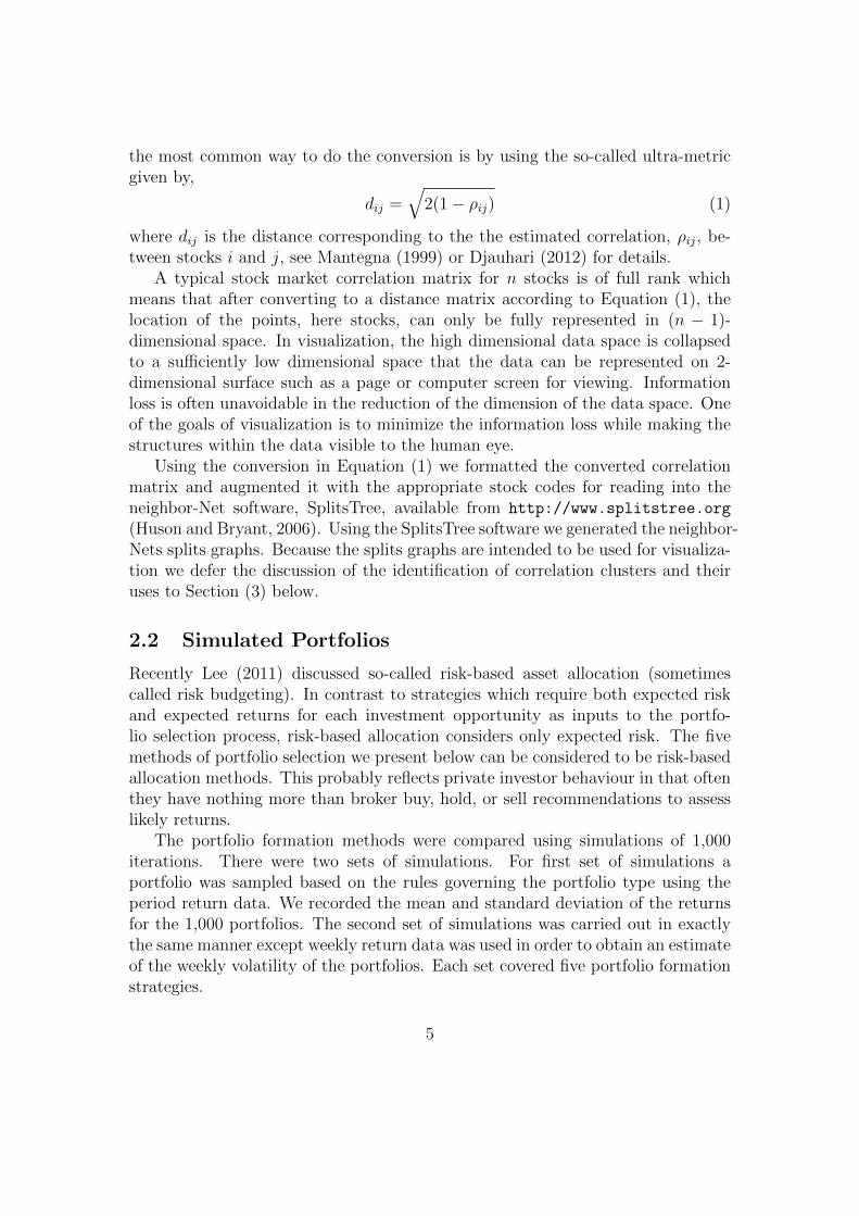
the most common way to do the conversion is by using the so-called ultra-metricgiven by,

dij =√

2(1− ρij) (1)

where dij is the distance corresponding to the the estimated correlation, ρij, be-tween stocks i and j, see Mantegna (1999) or Djauhari (2012) for details.

A typical stock market correlation matrix for n stocks is of full rank whichmeans that after converting to a distance matrix according to Equation (1), thelocation of the points, here stocks, can only be fully represented in (n − 1)-dimensional space. In visualization, the high dimensional data space is collapsedto a sufficiently low dimensional space that the data can be represented on 2-dimensional surface such as a page or computer screen for viewing. Informationloss is often unavoidable in the reduction of the dimension of the data space. Oneof the goals of visualization is to minimize the information loss while making thestructures within the data visible to the human eye.

Using the conversion in Equation (1) we formatted the converted correlationmatrix and augmented it with the appropriate stock codes for reading into theneighbor-Net software, SplitsTree, available from http://www.splitstree.org

(Huson and Bryant, 2006). Using the SplitsTree software we generated the neighbor-Nets splits graphs. Because the splits graphs are intended to be used for visualiza-tion we defer the discussion of the identification of correlation clusters and theiruses to Section (3) below.

2.2 Simulated Portfolios

Recently Lee (2011) discussed so-called risk-based asset allocation (sometimescalled risk budgeting). In contrast to strategies which require both expected riskand expected returns for each investment opportunity as inputs to the portfo-lio selection process, risk-based allocation considers only expected risk. The fivemethods of portfolio selection we present below can be considered to be risk-basedallocation methods. This probably reflects private investor behaviour in that oftenthey have nothing more than broker buy, hold, or sell recommendations to assesslikely returns.

The portfolio formation methods were compared using simulations of 1,000iterations. There were two sets of simulations. For first set of simulations aportfolio was sampled based on the rules governing the portfolio type using theperiod return data. We recorded the mean and standard deviation of the returnsfor the 1,000 portfolios. The second set of simulations was carried out in exactlythe same manner except weekly return data was used in order to obtain an estimateof the weekly volatility of the portfolios. Each set covered five portfolio formationstrategies.

5

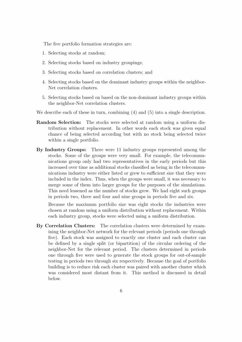
The five portfolio formation strategies are:

1. Selecting stocks at random;

2. Selecting stocks based on industry groupings;

3. Selecting stocks based on correlation clusters; and

4. Selecting stocks based on the dominant industry groups within the neighbor-Net correlation clusters.

5. Selecting stocks based on based on the non-dominant industry groups withinthe neighbor-Net correlation clusters.

We describe each of these in turn, combining (4) and (5) into a single description.

Random Selection: The stocks were selected at random using a uniform dis-tribution without replacement. In other words each stock was given equalchance of being selected according but with no stock being selected twicewithin a single portfolio.

By Industry Groups: There were 11 industry groups represented among thestocks. Some of the groups were very small. For example, the telecommu-nications group only had two representatives in the early periods but thisincreased over time as additional stocks classified as being in the telecommu-nications industry were either listed or grew to sufficient size that they wereincluded in the index. Thus, when the groups were small, it was necessary tomerge some of them into larger groups for the purposes of the simulations.This need lessened as the number of stocks grew. We had eight such groupsin periods two, three and four and nine groups in periods five and six.

Because the maximum portfolio size was eight stocks the industries werechosen at random using a uniform distribution without replacement. Withineach industry group, stocks were selected using a uniform distribution.

By Correlation Clusters: The correlation clusters were determined by exam-ining the neighbor-Net network for the relevant periods (periods one throughfive). Each stock was assigned to exactly one cluster and each cluster canbe defined by a single split (or bipartition) of the circular ordering of theneighbor-Net for the relevant period. The clusters determined in periodsone through five were used to generate the stock groups for out-of-sampletesting in periods two through six respectively. Because the goal of portfoliobuilding is to reduce risk each cluster was paired with another cluster whichwas considered most distant from it. This method is discussed in detailbelow.

6

If there were fewer clusters than the desired portfolio size, cluster pairs wereselected at random and a stock selected from within each correlation clusterpair. The simulation code was written so that if the desired portfolio sizewas larger than the number of correlation clusters then each cluster grouppair had at least s stocks selected, where s is the quotient of the portfoliosize divided by the number of clusters. Some (the remainder of the portfoliosize divided by number of clusters) correlation groups will have s+ 1 stocksselected and the cluster pairs this applied to were chosen using a uniform dis-tribution without replacement. However, in all cases the number of clustersequalled or exceeded the number of stocks in the simulated portfolios.

By Dominant or Non-Dominant Industry Group within Clusters: The fi-nal two methods relate to selecting stocks from industry groups within cor-relation clusters. Each stock within each cluster has an associated industrygroup. Therefore each correlation cluster can be subdivided into up to elevensub-clusters based on industry. However, it was clear that in a number ofclusters one industry was dominant, sometimes more than half of the stocks.This lead us to assign each stock to either the dominant industry group orthe non-dominant industry grouping creating two groups of stocks withineach cluster. This created two disjoint sets of clusters with no stock in bothgroups.

From these two distinct sets of stocks, simulations were run in the samemanner as that described in “By Correlation Clusters” above. These simu-lations were not comparable with the three above because the sample sizeswere different and, obviously, each deals with a subset of the data. However,care was taken to ensure that the sample sizes of both subsets was as closeto equal in size as was practical.

A problem arose, particularly with the non-dominant industry group stockswhen the number of stocks in the cluster was considered too small. In thesecases we took advantage of the circular ordering produced by neighbor-Netsand combined the small cluster with a neighbouring cluster.

Unchanged from above, each cluster was paired with the one most distantfrom it. Once a cluster was selected for inclusion, so was the paired cluster,and a selection was made using a uniform distribution and, if necessary,without replacement.

All simulations were coded and run in R (R Core Team, 2014).We used the stocks weekly return data in period one to determine the clusters,

then observed period two’s return distributions of the simulated portfolios (1000replications) which are picked from the different correlation clusters. Because out-of-sample testing was used in our analysis, the simulation then was continued for

7

period three, four, five and six based on the graphs produced from the weeklyreturns in period two, three, four and five respectively.

3 Neighbor-Net Splits Graphs

For three of the five types of portfolio simulation methods discussed above we needto identify correlation clusters from the neighbor-Net splits graphs. In this sectionwe explain how to identify the clusters, then proceed to present the neighbor-Netsplits graphs and the clusters identified for each of the first five periods.

At its simplest a neighbor-Net splits graph is a type of map. The ability toidentify correlation clusters depends on the user’s skill in reading it. As an analogy,all readers of a topographic map read the map in the same way. The informationthe reader extracts depends on their needs. One person may read a map to extractinformation about mountain ranges, another for information on river catchments,and still another on the distribution of human settlements. But in all cases themap readers agree which features are mountains, which are rivers and which aretowns and cities, no confusion arises because the map is read visually. In the sameway all readers of neighbor-Net splits graphs agree on which feature or features arethe origin, which are splits, which are recombinations and which are the terminallocations.

Because this is a visual approach, the information extracted from reading aneighbor-Net splits graph depends on the researcher or financial analyst balancingwhatever competing requirements they may have. Here we know that in the sim-ulations to follow the sizes of the portfolios we will generate will be two, four, oreight stocks. Consequently, we do not need large numbers of clusters and we wouldlike them to have a sufficiently large number of stocks such that when selectingstocks at random from within the cluster there are a sufficiently large number ofcombinations available to make the simulations meaningful. These requirementsguide us when identifying clusters in the neighbor-Net splits graphs. The numbersof clusters and cluster membership is determined visually and it is important notto confuse visual with subjective.

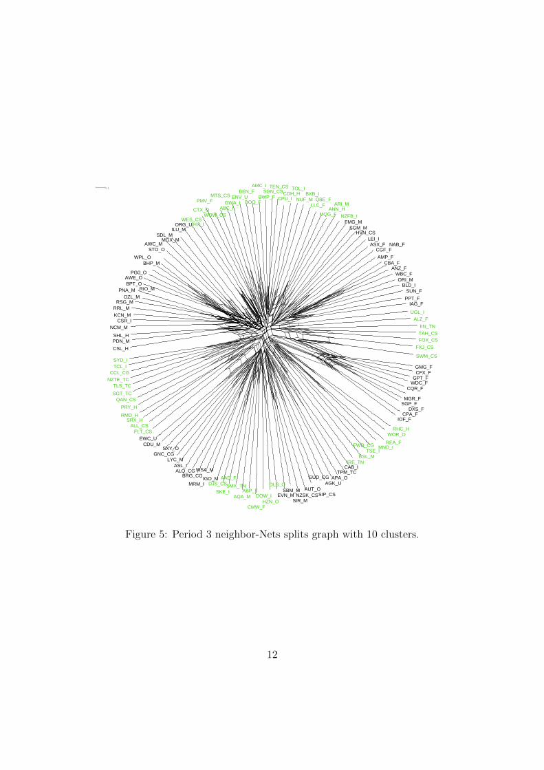
Figures (2) through (8) present the neighbor-Nets splits graphs for periods onethrough five. These were used to determine the stock groups for out-of-sampletesting using data from periods two through six respectively.

In Figure (2) eight clusters were identified and are colour coded in order todistinguish them. The SplitsTree software generates a large amount of statisticalinformation about the network. However, we, like other users of neighbor-Nets,look for breaks in the structure of the network. A good example can be found atabout eight o’clock in the splits graph between the stocks labelled CMW F andCPA F. In its original context of phylogenetics, if these were species it would tell

8

us that the last common ancestor was in the distant past. Although CMW F andCPA F are placed next to each other in the circular ordering, the two stocks arenot closely related.

FOX_CSBHP_MRIO_MAWC_M

TEN_CS

MGX_MCAB_I

SGM_M

MND_ICDU_M

MTS_CSNUF_MORI_M

IIN_TNUGL_I

CGF_FSMX_TN

ASX_F

CPU_F

REA_FMRM_I

EWC_UPMV_F

ORG_UPG0_O

WPL_O

ILU_M

CTX_O

ALQ_CG

PRY_HANN_H

HZN_OFMG_M

NZSK_CS

AWE_OWDC_F

ENV_U

BPT_OPDN_M

CCL_CGDJS_CS

SDL_MAGK_U

ASL_IAAD_F

TCL_ICMW_F

CPA_F

CFX_FMGR_FSGP_F

GPT_FDXS_F

IOF_F

BWP_F

CQR_F

RRL_M

TLS_TC

NZTE_TC

TAH_CS

WOW_CS

AUT_O

KCN_M

SGN_CSSBM_M

RSG_MNCM_M

SIR_MOZL_M

BRG_CGFWD_CG

GUD_CG

DLS_OALZ_F

GMG_FLYC_M

PNA_M

GWA_IBLD_I

QBE_F

JHX_ICSR_I

SUN_F

CBA_FNAB_F

ANZ_F

WBC_FGNC_CG

BOQ_FRHC_H

STO_O

CSL_H

COH_HRMD_H

TOL_ILEI_I

WES_CSALL_CS

HVN_CSMQG_F

AMP_FSWM_CS

FLT_CSPPT_F

BEN_FSHL_HDOW_IABC_I

SKE_I

LLC_FSXY_O

BXB_IQAN_CS

AMC_I

FXJ_CS

0.1

Figure 2: Period 1 neighbor-Nets splits graph with eight clusters identified.

Figure (3) presents the same splits graph but within each cluster the stocks aresplit into stocks which belong to the dominant industry group (larger typeface)and stocks which are in other groups (smaller typeface). For example, in the aquacoloured group, the dominant industry is financials and all but three stocks belongto this sector.

Figure (4) presents the neighbor-Nets splits graph for period 2. While theclusters in this figure have not been visually separated into dominant and non-dominate industry groups, the cluster between nine and ten o’clock is dominatedby financial stocks. It is also straight-forward to see how the clusters were paired.

9

FOX_CS

BHP_MRIO_MAWC_M

TEN_CS

MGX_MCAB_I

SGM_M

MND_I

CDU_MMTS_CS

NUF_MORI_M

IIN_TN

UGL_I

CGF_F

SMX_TNASX_F

CPU_F

REA_FMRM_I

EWC_UPMV_F

ORG_U

PG0_OWPL_O

ILU_MCTX_O

ALQ_CGPRY_H

ANN_H

HZN_OFMG_M

NZSK_CS

AWE_OWDC_F

ENV_UBPT_O

PDN_MCCL_CG

DJS_CSSDL_M

AGK_U

ASL_IAAD_F

TCL_ICMW_F

CPA_FCFX_F

MGR_F

SGP_FGPT_FDXS_F

IOF_F

BWP_F

CQR_F

RRL_M

TLS_TC

NZTE_TC

TAH_CS

WOW_CS

AUT_O

KCN_M

SGN_CS

SBM_M

RSG_MNCM_M

SIR_MOZL_M

BRG_CG

FWD_CG

GUD_CG

DLS_OALZ_F

GMG_FLYC_M

PNA_M

GWA_IBLD_I

QBE_FJHX_I

CSR_ISUN_F

CBA_F

NAB_FANZ_F

WBC_FGNC_CG

BOQ_FRHC_H

STO_OCSL_H

COH_HRMD_H

TOL_ILEI_I

WES_CSALL_CS

HVN_CSMQG_F

AMP_F

SWM_CS

FLT_CSPPT_F

BEN_F

SHL_H

DOW_I

ABC_I

SKE_I

LLC_F

SXY_O

BXB_I

QAN_CS

AMC_I

FXJ_CS

0.1

Figure 3: Period 1 neighbor-Nets splits graph with the clusters split into dominantand non-dominant industries.

The cluster just mentioned would be paired with the black coloured cluster betweenabout 2:30 and 3:30 on the opposite side of the network. These stocks are the mostdistant in terms of the circular ordering. If the correlation clusters represent usefulfinancial groupings of stocks we would expect that choosing a pair of stocks fromthese two clusters would be likely to give a greater reduction in risk than twostocks selected randomly.

10

FOX_CS

FXJ_CS

ENV_U

PDN_M

REA_F

NZFB_INZTE_TC

SMX_TN

MRM_INZSK_CS

SRX_HABC_I

SIP_CSSYD_I

EWC_U

MTS_CS

APA_OMGX_M

CTX_OSDL_M

CCL_CGAGK_U

WOW_CS

AAD_F

ANN_HCSL_H

ALL_CSCOH_H

ASL_I

PPT_FCPU_F

TOL_IIAG_F

LEI_ITSE_I

DOW_IWOR_O

TEN_CSSWM_CS

BXB_I

AMC_ICGF_F

ASX_F

AWC_M

RIO_MBHP_M

ARI_MBSL_M

BLD_IJHX_I

CSR_ISGM_M

ORG_USHL_H

WES_CS

NUF_MORI_M

DJS_CSQAN_CSHVN_CS

EVN_MFLT_CS

FWD_CGSGN_CS

SKE_I

ALZ_F

BWP_F

MGR_F

SGP_FCFX_FIOF_FCPA_FCQR_F

DXS_F

GPT_F

CBA_FWBC_F

ANZ_FNAB_F

BOQ_FSUN_F

QBE_F

TAH_CS

WDC_FMQG_F

AUT_OILU_MSTO_O

IRE_TN

FMG_MAQA_M

CMW_FLYC_M

IIN_TN

ALQ_CGPRY_H

TPM_TC

PG0_O

WPL_OAWE_O

UGL_I

CAB_IAMP_F

LLC_FTCL_I

ABP_FMND_I

BPT_OHZN_O

DLS_OSXY_O

GNC_CGPNA_M

RSG_MOZL_M

NCM_MSIR_M

KCN_M

SBM_MRRL_M

PMV_FBRG_CG

GUD_CGGWA_I

BEN_FCDU_MRHC_H

IGO_M

WSA_M

TLS_TC

GMG_FSGT_TCRMD_H

0.1

Figure 4: Period 2 neighbor-Nets splits graph with 10 clusters.

11

FOX_CS

FXJ_CS

SWM_CS

GMG_FCFX_F

GPT_FWDC_F

CQR_F

DXS_F

MGR_FSGP_F

CPA_FIOF_F

RHC_HWOR_O

REA_FMND_I

TSE_IBSL_M

FWD_CG

IRE_TNCAB_I

TPM_TCAPA_O

AGK_U

SIP_CS

GUD_CG

AUT_ONZSK_CS

SIR_M

SBM_MEVN_M

DLS_O

HZN_ODOW_I

CMW_F

ABP_FAQA_M

SMX_TN

AAD_F

SKE_I

DJS_CSIGO_M

WSA_M

MRM_I

BRG_CGALQ_CG

ASL_ILYC_M

SXY_OGNC_CG

CDU_MEWC_U

FLT_CSALL_CS

SRX_HRMD_H

PRY_H

QAN_CSSGT_TC

TLS_TCNZTE_TCCCL_CG

TCL_ISYD_I

CSL_H

PDN_MSHL_H

NCM_MCSR_I

KCN_MRRL_M

RSG_MOZL_M

PNA_MBPT_OAWE_O

PG0_O

WPL_O

RIO_M

BHP_M

AWC_MSTO_O

SDL_MMGX_M

ILU_MORG_U

WES_CSJHX_I

CTX_O

PMV_F

WOW_CS

MTS_CS

ABC_IGWA_I

ENV_UBEN_F

BOQ_F

AMC_I

BWP_FSGN_CS

TEN_CS

CPU_ICOH_H

TOL_I

NUF_MBXB_I

LLC_FQBE_F

MQG_FANN_H

ARI_M

NZFB_IFMG_M

SGM_MHVN_CS

LEI_IASX_F

CGF_F

AMP_FCBA_F

NAB_F

ANZ_FWBC_FORI_M

BLD_ISUN_F

PPT_FIAG_F

UGL_IALZ_F

IIN_TNTAH_CS

0.1


12

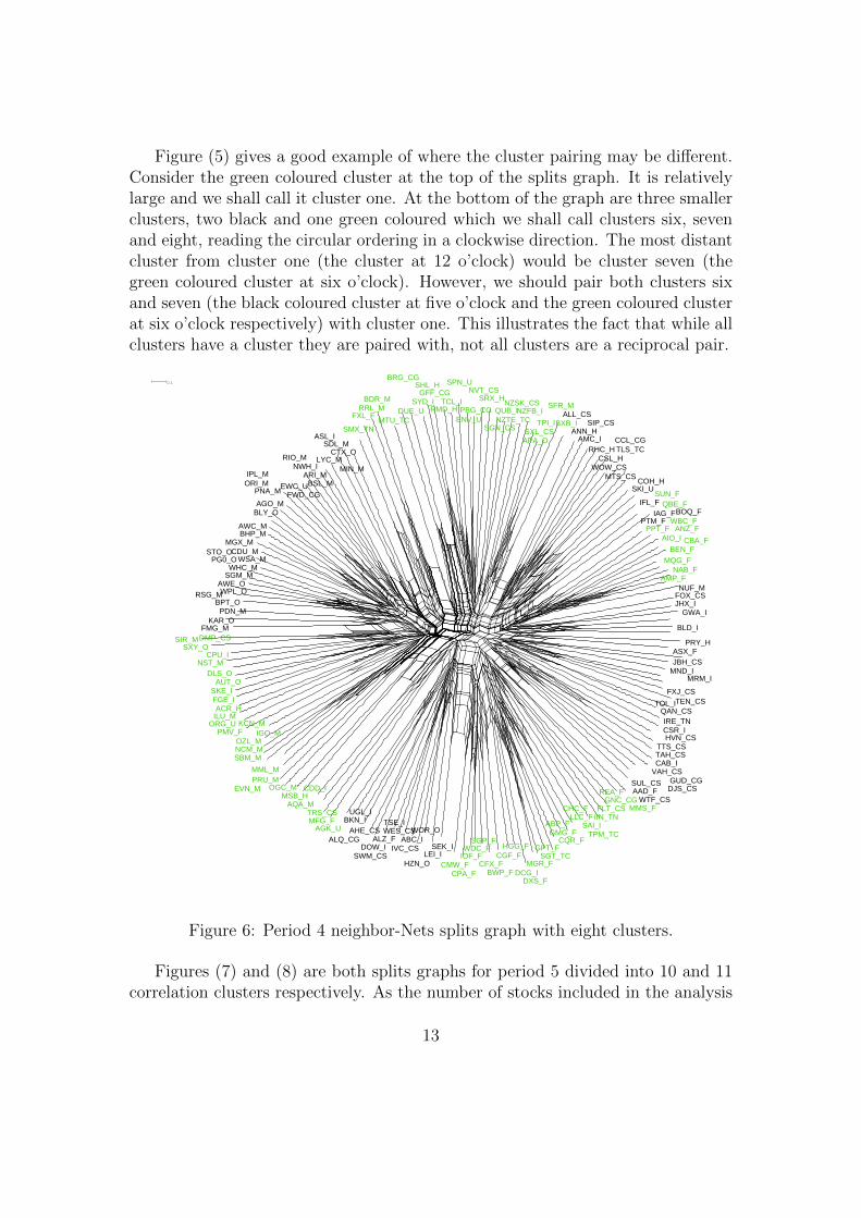
Figure (5) gives a good example of where the cluster pairing may be different.Consider the green coloured cluster at the top of the splits graph. It is relativelylarge and we shall call it cluster one. At the bottom of the graph are three smallerclusters, two black and one green coloured which we shall call clusters six, sevenand eight, reading the circular ordering in a clockwise direction. The most distantcluster from cluster one (the cluster at 12 o’clock) would be cluster seven (thegreen coloured cluster at six o’clock). However, we should pair both clusters sixand seven (the black coloured cluster at five o’clock and the green coloured clusterat six o’clock respectively) with cluster one. This illustrates the fact that while allclusters have a cluster they are paired with, not all clusters are a reciprocal pair.

FOX_CS

PRY_HASX_F

MRM_I

JBH_CSMND_I

HVN_CS

DJS_CS

FXJ_CSTEN_CS

GUD_CG

QAN_CSIRE_TNCSR_I

TOL_I

TTS_CSTAH_CSCAB_I

VAH_CS

WTF_CSAAD_FSUL_CS

MMS_FGNC_CG

FLT_CS

REA_F

IIN_TN

TPM_TCSAI_I

LLC_FCHC_F

CQR_FGMG_F

ABP_F

SGT_TCGPT_F

MGR_F

DXS_FDCG_I

HGG_FCGF_F

BWP_FCFX_F

SGP_FWDC_F

IOF_F

CPA_FCMW_F

SEK_ILEI_I

WOR_O

HZN_O

ABC_IIVC_CS

WES_CSTSE_I

ALZ_FDOW_I

SWM_CS

AHE_CS

UGL_IBKN_I

ALQ_CGAGK_U

MFG_FTRS_CS

CDD_I

AQA_MMSB_H

OGC_MPRU_MMML_M

IGO_M

NCM_MSBM_M

EVN_M

OZL_M

KCN_MPMV_F

ACR_HILU_M

ORG_U

FGE_ISKE_I

AUT_ODLS_O

DMP_CS

NST_MCPU_I

SXY_OSIR_M

FMG_M

RSG_M

KAR_O

BPT_O

PG0_OSTO_O

AWE_OWPL_O

PDN_M

WHC_MSGM_M

CDU_MMGX_M

WSA_M

BHP_MAWC_M

ORI_MIPL_M

BLY_OAGO_M

PNA_MEWC_U

RIO_M

FWD_CG

NWH_IARI_M

BSL_M

ASL_I

LYC_M

SDL_MCTX_O

MIN_M

SMX_TN

FXL_FRRL_M

BDR_M

MTU_TC

BRG_CG

DUE_USYD_I

SHL_HGFF_CG

RMD_HTCL_I

SPN_U

ENV_UPBG_CG

NVT_CSSRX_H

SGN_CS

QUB_INZTE_TC

NZSK_CSNZFB_I

APA_OSXL_CS

TPI_I

SFR_M

BXB_IALL_CS

ANN_HAMC_I

SIP_CS

RHC_HCSL_H

WOW_CSMTS_CS

CCL_CGTLS_TC

SKI_UCOH_H

IFL_F

PTM_FIAG_F

PPT_F

SUN_F

AIO_I

QBE_F

BEN_F

AMP_F

MQG_FNAB_F

ANZ_FWBC_F

CBA_F

NUF_M

BOQ_F

GWA_IJHX_I

BLD_I

0.1

Figure 6: Period 4 neighbor-Nets splits graph with eight clusters.

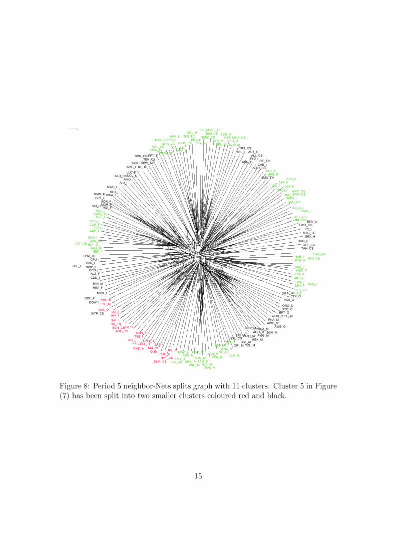
Figures (7) and (8) are both splits graphs for period 5 divided into 10 and 11correlation clusters respectively. As the number of stocks included in the analysis

13

FOX_CS

FXJ_CSPTM_FNAB_FANZ_FWBC_F

CBA_F

SUN_FAMP_F

BOQ_FBEN_FTTS_CS

ASX_F

CTX_OPG0_O

WPL_O

ORG_USTO_O

ILU_MBPT_O

AWE_O

WOR_O

PNA_MAWC_M

SGM_MWSA_M

FMG_MAGO_M

MGX_MBHP_M

RIO_M

OZL_M

BSL_M

ARI_MORI_M

SXL_CS

ACR_HHZN_O

WHC_M

IVC_CS

IGO_M

PDN_MKCN_M

EVN_MSLR_M

SBM_MNCM_M

OGC_MPRU_M

MML_M

RSG_MEWC_U

KAR_O

PBG_CG

IPL_M

NVT_CS

RHC_HDMP_CS

SKE_IQUB_I

SDL_MCOH_H

CSL_HRMD_H

MMS_FTSE_I

FGE_I

ASL_IFXL_F

AHE_CS

SGN_CSIIN_TN

SAI_I

JHX_ILEI_I

CDU_M

DLS_O

LYC_MDOW_I

QBE_F MRM_I

WTF_CSREA_FMIN_M

DCG_I

CDD_IALZ_F

BWP_F

TOL_IAAD_F

CPU_ITPM_TC

SEK_IAQA_M

FLT_CSBLY_OBKN_I

QAN_CSABC_I

CSR_ICQR_FCHC_F

MQG_FCGF_F

CWN_CS

SKI_UGMG_F

GPT_F

SGP_FMGR_F

IOF_F

GWA_IBLD_I

NWH_IALQ_CG

AIO_IMND_I

UGL_ILLC_F

AMC_IBXB_I

IFL_F

BRG_CGSWM_CS

TEN_CS

PPT_F

CMW_F

SUL_CSMSB_H

WOW_CS

MTS_CS

SPN_UAGK_U

CCL_CG

APA_ONZTE_TC

TLS_TCSHL_H

PRY_HSXY_O

SIR_MNZSK_CS

GEM_CS

SGT_TC

SFR_MRRL_M

BDR_MNST_M

BRU_ONUF_M

SIP_CSTCL_I

TRS_CS

ANN_HAUT_O

SYD_IALL_CS

VAH_CS

CAB_I

IRE_TNSMX_TN

DUE_U

MFG_FIAG_F

ABP_F

WDC_FCFX_FCPA_F

DXS_FNZFB_I

GUD_CG

GNC_CG

HVN_CS

DJS_CSJBH_CS

WES_CS

PMV_F

ENV_U

FWD_CG

TPI_IMTU_TC

SRX_H

HGG_F

GFF_CGTAH_CS

0.1


grows the analyst gains some flexibility in choosing the number of clusters.To summarize, a stock market analyst or portfolio manager looks for breaks

in the structure of the neighbor-Net network when dividing the stocks into corre-lation clusters. The SplitsTree software has considerable flexibility to magnifysections of the network to aid in decision making which cannot be easily capturedin the static pdf file outputs included in this paper. The circular ordering can bevery useful when splitting a correlation cluster into its component industry groupsbecause if one or more of the resulting groups are too small to be useful they canbe joined with groups next to them in the circular order.

14

FOX_CS

FXJ_CSPTM_FNAB_F

ANZ_FWBC_F

CBA_F

SUN_FAMP_F

BOQ_FBEN_FTTS_CS

ASX_FCTX_O

PG0_O

WPL_O

ORG_USTO_O

ILU_MBPT_O

AWE_O

WOR_OPNA_M

AWC_M

SGM_MWSA_M

FMG_MAGO_M

MGX_M

BHP_M

RIO_M

OZL_MBSL_M

ARI_M

ORI_M

SXL_CS

ACR_H

HZN_O

WHC_MIVC_CS

IGO_M

PDN_MKCN_M

EVN_MSLR_M

SBM_MNCM_M

OGC_M

PRU_MMML_M

RSG_MEWC_U

KAR_OPBG_CG

IPL_M

NVT_CSRHC_H

DMP_CS

SKE_I

QUB_ISDL_M

COH_HCSL_H

RMD_H

MMS_FTSE_I

FGE_IASL_I

FXL_FAHE_CS

SGN_CSIIN_TNSAI_I

JHX_ILEI_I

CDU_M

DLS_O

LYC_MDOW_IQBE_F

MRM_I

WTF_CS

REA_FMIN_M

DCG_I

CDD_IALZ_F

BWP_FTOL_IAAD_F

CPU_ITPM_TC

SEK_IAQA_M

FLT_CS BLY_O

BKN_IQAN_CS

ABC_ICSR_I

CQR_FCHC_F

MQG_F

CGF_FCWN_CS

SKI_U

GMG_FGPT_F

SGP_FMGR_F

IOF_F

GWA_IBLD_I

NWH_I

ALQ_CG

AIO_IMND_I

UGL_ILLC_F

AMC_IBXB_I

IFL_F

BRG_CG

SWM_CSTEN_CS

PPT_F

CMW_FSUL_CS

MSB_H

WOW_CS

MTS_CSSPN_U

AGK_U

CCL_CGAPA_O

NZTE_TC

TLS_TCSHL_H

PRY_HSXY_O

SIR_M

NZSK_CSGEM_CS

SGT_TC

SFR_MRRL_M

BDR_MNST_M

BRU_ONUF_M

SIP_CS

TCL_ITRS_CS

ANN_H

AUT_O

SYD_IALL_CS

VAH_CSCAB_IIRE_TN

SMX_TN

DUE_UMFG_F

IAG_FABP_F

WDC_FCFX_F

CPA_F

DXS_FNZFB_I

GUD_CG

GNC_CGHVN_CS

DJS_CS

JBH_CSWES_CS

PMV_F

ENV_UFWD_CG

TPI_IMTU_TC

SRX_H

HGG_FGFF_CG

TAH_CS

0.1

Figure 8: Period 5 neighbor-Nets splits graph with 11 clusters. Cluster 5 in Figure(7) has been split into two smaller clusters coloured red and black.

15

Period 2 Neighbor-Nets Industry Correlation CorrelationSimulation Random correlation Group cluster with cluster withoutresults cluster industry group industry groupMean return(2-stock) 106.49 94.93 98.52 101.80 97.24(4-stock) 101.51 98.45 96.93 97.55 97.12(8-stock) 104.66 96.90 100.82 98.892 96.14Std. Dev.(2-stock) 79.34 *70.51 73.87 81.90 *62.47(4-stock) *49.39 51.85 48.96 53.14 *43.62(8-stock) *33.61 35.64 36.56 42.33 *29.81Sharpe Ratio(2-stock) 1.34 1.35 1.33 1.24 1.56(4-stock) 2.06 1.90 1.98 1.84 2.23(8-stock) 3.11 2.72 2.69 2.70 3.23Levene Tests(2-stock) 0.001 1.0× 10−7

(4-stock) 0.30 1.7× 10−6

(8-stock) 0.13 1.3× 10−12

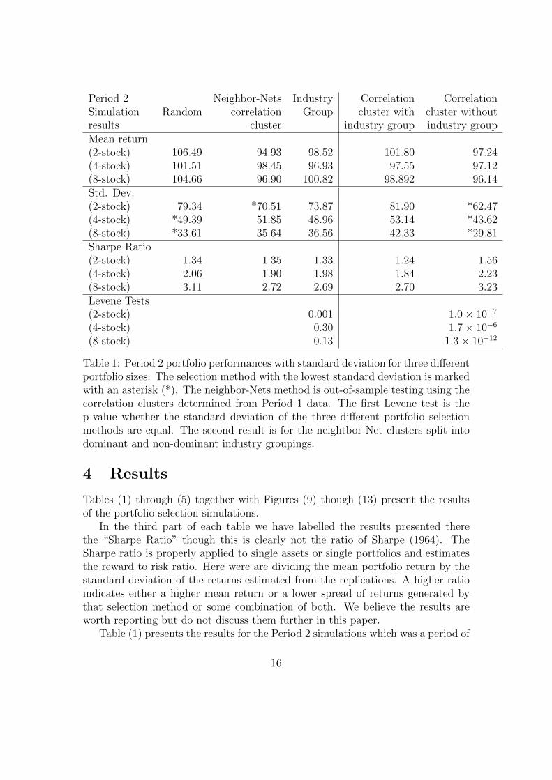
Table 1: Period 2 portfolio performances with standard deviation for three differentportfolio sizes. The selection method with the lowest standard deviation is markedwith an asterisk (*). The neighbor-Nets method is out-of-sample testing using thecorrelation clusters determined from Period 1 data. The first Levene test is thep-value whether the standard deviation of the three different portfolio selectionmethods are equal. The second result is for the neightbor-Net clusters split intodominant and non-dominant industry groupings.

4 Results

Tables (1) through (5) together with Figures (9) though (13) present the resultsof the portfolio selection simulations.

In the third part of each table we have labelled the results presented therethe “Sharpe Ratio” though this is clearly not the ratio of Sharpe (1964). TheSharpe ratio is properly applied to single assets or single portfolios and estimatesthe reward to risk ratio. Here were are dividing the mean portfolio return by thestandard deviation of the returns estimated from the replications. A higher ratioindicates either a higher mean return or a lower spread of returns generated bythat selection method or some combination of both. We believe the results areworth reporting but do not discuss them further in this paper.

Table (1) presents the results for the Period 2 simulations which was a period of

16

strongly rising equity prices. The model building period (Period 1) was a periodwhen the market largely tracked sideways with a small decline over the period.Thus the out-of-sample test represents a strong test of stock selection methodsbetween the two periods which do not resemble each other.

We are primarily concerned with reducing the risk of the portfolios. The resultsin the table give the standard deviation of the returns of the 1000 replications of theportfolio selection method. A lower standard deviation indicates that the returns ofthe portfolios were more concentrated about the mean portfolio return. The Levenetests show that only the two stock portfolios had a significantly different spread ofreturns. The difference between the random selection method and neighbor-Netsselection was almost nine percentage points different.

The final two columns of Table (1) present the results for the simulationsin which the correlation clusters were divided into dominant and non-dominantindustry groups. In this case the correlation clusters of non-dominant industriesshowed statistically significantly lower levels of spread of the portfolio returns.

Figure (9) plots the returns of the weekly standard deviation of the portfolioreturns, a measure of volatility, against the period portfolio return for the eight-stock portfolios dividing the stocks in to dominant and non-dominant industrygroups. The differences are not pronounced but the spread of returns is smallerfor the correlation clusters with non-dominant industry groups though the weeklyvolatility appears comparable.

Table (2) presents the results for the Period 3 simulations which was a periodof strongly rising equity prices. The model building period (Period 2) was alsoa period of market increases. Thus the out-of-sample test and model buildingperiods closely resemble each other.

The Levene tests show that only the two stock portfolios had a significantlydifferent spread of returns, though the results for the eight-stock portfolios almostreached statistical significance. The difference between the neighbor-Nets selectionand industry group selection was almost 10 percentage points different.

The final two columns of Table (2) present the results for the simulationsin which the correlation clusters were divided into dominant and non-dominantindustry groups. In this case the correlation clusters of the dominant industriesshowed statistically significantly lower levels of spread of the portfolio returns.

Figure (10) plots the returns of the weekly standard deviation of the portfolioreturns, a measure of volatility, against the period portfolio return for the eight-stock portfolios dividing the stocks in to dominant and non-dominant industrygroups. It is noticeable that the spread of returns is smaller for the correlationclusters with dominant industry groups though the weekly volatility is higher.

Table (3) presents the result for the Period 4 simulations. Period four wasa period of strongly falling equity prices. The model building period (Period 3)

17

Period 3 Neighbor-Nets Industry Correlation CorrelationSimulation Random correlation Group cluster with cluster withoutresults cluster industry group industry groupMean return(2-stock) 156.32 149.30 135.11 137.09 150.97(4-stock) 152.99 151.27 134.02 132.85 155.49(8-stock) 154.30 149.05 137.79 134.82 152.94Std. Dev.(2-stock) 108.11 109.64 *99.57 *66.02 116.40(4-stock) 75.93 75.47 *71.01 *45.62 83.45(8-stock) 51.34 50.15 *48.26 *32.49 57.63Sharpe Ratio(2-stock) 1.45 1.36 1.36 2.07 1.27(4-stock) 2.01 2.00 1.89 2.91 1.86(8-stock) 3.01 2.97 2.86 4.15 2.65Levene Tests(2-stock) 0.05 < 10−16

(4-stock) 0.15 < 10−16

(8-stock) 0.06 < 10−16


18

Period 4 Neighbor-Nets Industry Correlation CorrelationSimulation Random correlation Group cluster with cluster withoutresults cluster industry group industry groupMean return(2-stock) -46.58 -49.18 -45.56 -54.61 -43.26(4-stock) -47.52 -49.46 -43.93 -54.81 -42.19(8-stock) -47.48 -48.52 -44.09 -54.70 -42.18Std. Dev.(2-stock) 22.80 *21.30 21.70 *17.16 23.49(4-stock) *15.16 15.41 15.68 *11.29 16.80(8-stock) 10.65 10.49 *10.42 *8.03 11.11Sharpe Ratio(2-stock) -2.04 -2.31 -2.10 -3.18 -1.85(4-stock) -3.13 -3.21 -2.80 -4.85 -2.51(8-stock) -4.46 -4.62 -4.25 -6.81 -3.80Levene Tests(2-stock) 0.78 1.6× 10−9

(4-stock) 0.32 < 10−16

(8-stock) 0.73 < 10−16


19

was a period of strong market increases. Thus the out-of-sample test and modelbuilding periods are effectively opposites of each other.

The Levene tests show that no stock portfolios had a significantly differentspread of returns.

The final two columns of Table (3) present the results for the simulationsin which the correlation clusters were divided into dominant and non-dominantindustry groups. In this case the correlation clusters of the dominant industriesshowed statistically significantly lower levels of spread of the portfolio returns. TheLevene tests were highly significant for all portfolio sizes.

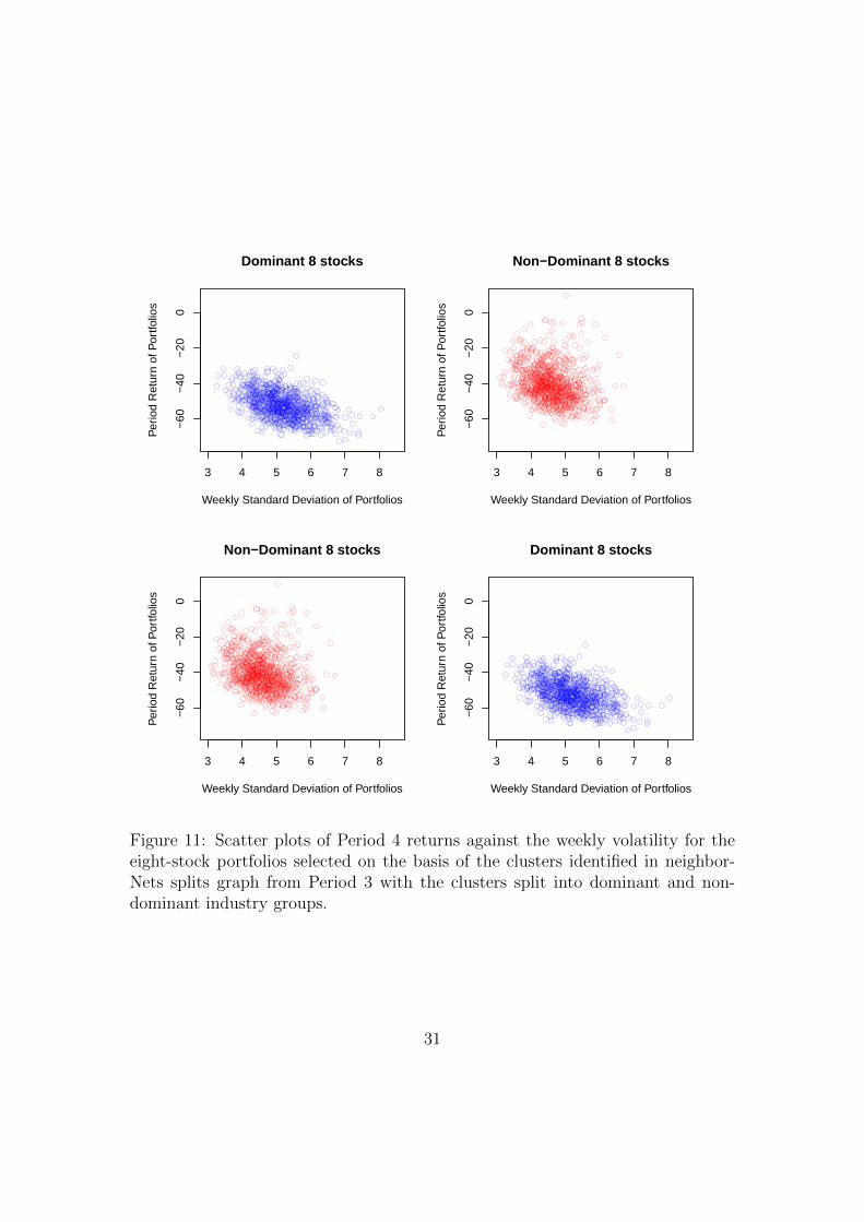
Figure (11) plots the returns of the weekly standard deviation of the portfolioreturns against the period portfolio return for the eight-stock portfolios dividingthe stocks in to dominant and non-dominant industry groups. It is noticeablethat the spread of returns is substantially smaller for the correlation clusters withdominant industry groups though, again, the weekly volatility is higher.

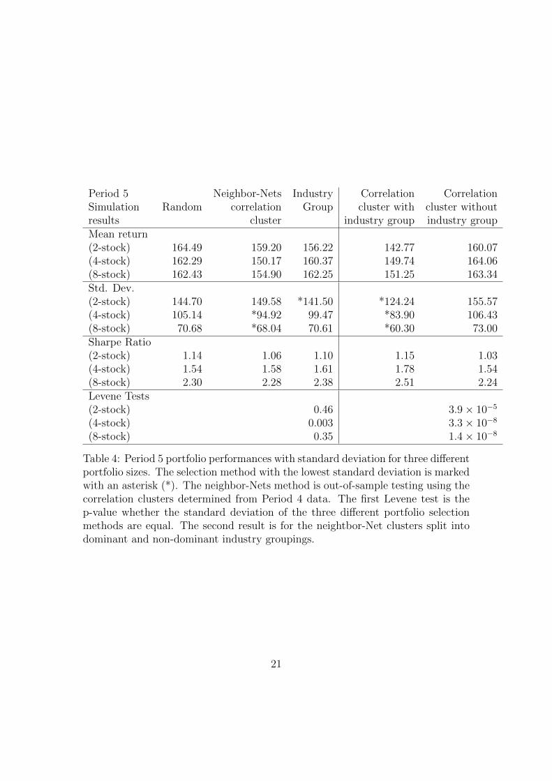
Table (4) presents the results for the Period 5 simulations which was a periodof equity prices initially rebounding then tracking sideways. The model buildingperiod (Period 4) was a period of strong market decreases. Thus the out-of-sampletest and model building periods are substantially different.

The Levene tests show that only the four stock portfolios had a significantlydifferent spread of returns.

The final two columns of Table (4) present the results for the simulationsin which the correlation clusters were divided into dominant and non-dominantindustry groups. In this case the correlation clusters of the dominant industriesshowed statistically significantly lower levels of spread of the portfolio returns. TheLevene tests were strongly significant for all portofilos sizes.

Figure (12) plots the returns of the weekly standard deviation of the portfolioreturns against the period portfolio return for the eight-stock portfolios dividingthe stocks in to dominant and non-dominant industry groups. It is noticeable thatthe spread of returns is smaller for the correlation clusters with dominant industrygroups though, again, the weekly volatility is higher.

Table (5) presents the result for the Period 6 simulations which was a period ofrising equity prices with significant volatility. The model building period (Period5) was a period of rebound followed by a time of stacking sideways. Thus theout-of-sample test and model building periods have some similarities.

The Levene tests show that the four and eight stock portfolios had a sig-nificantly different spread of returns. In both cases the neighbor-Nets portfolioselection method had the lowest spread of returns.

The final two columns of Table (5) present the results for the simulationsin which the correlation clusters were divided into dominant and non-dominantindustry groups. In this case the correlation clusters of the dominant industries

20

Period 5 Neighbor-Nets Industry Correlation CorrelationSimulation Random correlation Group cluster with cluster withoutresults cluster industry group industry groupMean return(2-stock) 164.49 159.20 156.22 142.77 160.07(4-stock) 162.29 150.17 160.37 149.74 164.06(8-stock) 162.43 154.90 162.25 151.25 163.34Std. Dev.(2-stock) 144.70 149.58 *141.50 *124.24 155.57(4-stock) 105.14 *94.92 99.47 *83.90 106.43(8-stock) 70.68 *68.04 70.61 *60.30 73.00Sharpe Ratio(2-stock) 1.14 1.06 1.10 1.15 1.03(4-stock) 1.54 1.58 1.61 1.78 1.54(8-stock) 2.30 2.28 2.38 2.51 2.24Levene Tests(2-stock) 0.46 3.9× 10−5

(4-stock) 0.003 3.3× 10−8

(8-stock) 0.35 1.4× 10−8


21

Period 6 Neighbor-Nets Industry Correlation CorrelationSimulation Random correlation Group cluster with cluster withoutresults cluster industry group industry groupMean return(2-stock) 45.96 46.60 54.36 34.77 65.16(4-stock) 48.39 51.10 55.19 35.85 61.87(8-stock) 46.66 50.32 55.62 35.36 62.09Std. Dev.(2-stock) 52.03 *49.87 51.62 *44.92 51.32(4-stock) 37.28 *33.18 34.11 *28.49 35.65(8-stock) 25.56 *21.63 22.94 *15.04 24.04Sharpe Ratio(2-stock) 0.88 0.93 1.05 0.77 1.27(4-stock) 1.30 1.54 1.62 1.26 1.74(8-stock) 1.76 2.33 2.42 2.35 2.58Levene Tests(2-stock) 0.64 0.004(4-stock) 0.007 4.0× 10−9

(8-stock) 1.1× 10−9 < 10−16


22

showed statistically significantly lower levels of spread of the portfolio returns. TheLevene tests were highly significant for all portofilos sizes.

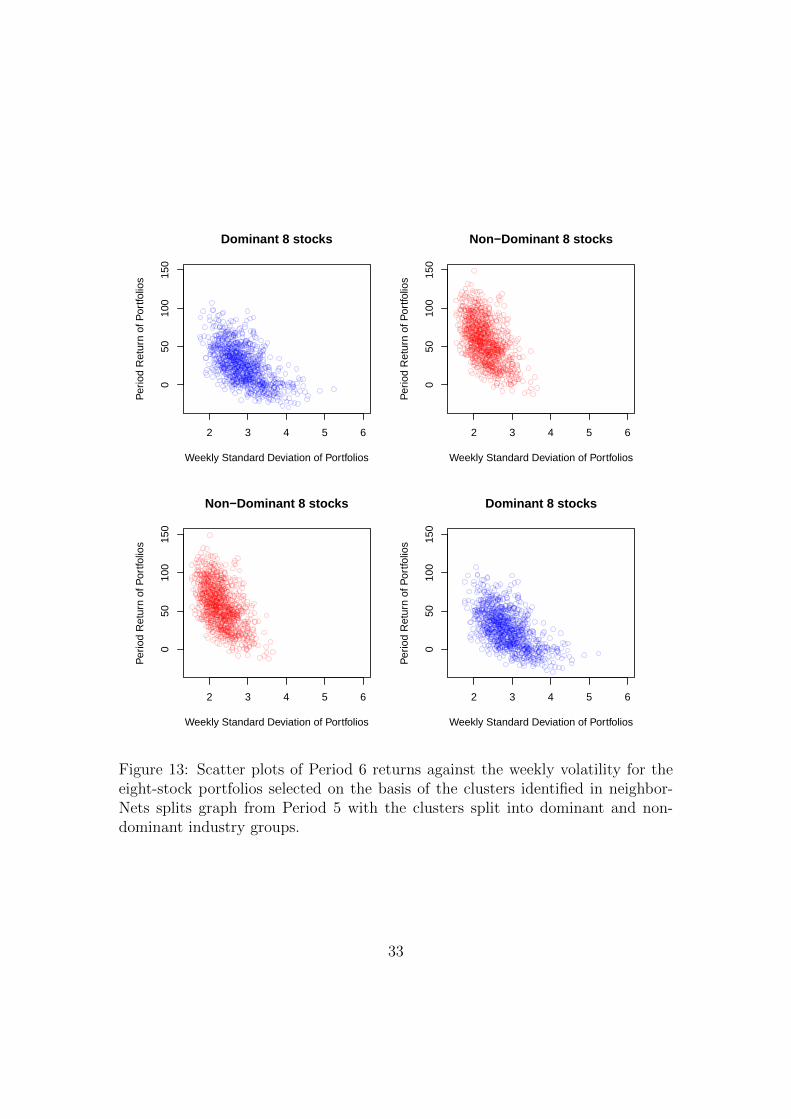
Figure (13) plots the returns of the weekly standard deviation of the portfolioreturns against the period portfolio return for the eight-stock portfolios dividingthe stocks in to dominant and non-dominant industry groups. It is noticeable thatthe spread of returns is smaller for the correlation clusters with dominant industrygroups though, as with some previous periods, the weekly volatility is higher.

5 Discussion and Conclusions

The simulation tests performed here represent a particularly severe test of portfoliodiversification because of the long out-of-sample test periods coupled with the factthat the market conditions in the model building phase were often very differentfrom the market conditions in the test phase.

In the 15 sets of simulations comparing, random, industry group, and neighbor-Net correlation cluster selection methods, statistically significant differences in theportfolios standard deviation were obtained only five times. In four cases theneighbor-Net correlation cluster produced the lowest standard deviation and inone case the industry group selection method was the lowest.

Considering the neighbor-Net correlation clusters split into dominant and non-dominant industries, all 15 cases had statistically significant differences in theportfolios’ standard deviation. Of these 12 were correlation clusters with dominantindustry groups in Periods 3 through 6 and three were correlation clusters withnon-dominant industry groups in Period 2. Because we do not have data frombefore the inception date of the ASX200 index it is not possible to say if thisrepresents a change in the behaviour of the market.

Figures (9) through (13) present this last observation in graphical form and it isclear that the distribution both in terms of portfolio returns and weekly volatilityare different for all periods. Graphs of the two and four stock portfolios showsimilar results but are not reported here.

These results suggest that within each correlation cluster there are two distinctsub-populations of stocks. Intuitively, the dominant industry group are simplystocks within the same industry with similar risk characteristics. We would expectsuch stocks to be strongly correlated, hence fall into the same correlation cluster.We would also expect that they would continue to be strongly correlated into thefuture. On the other hand, the stocks in the non-dominant industry group withina correlation cluster would seem far less likely to remain strongly correlated in thefuture.

At this stage we can only recommend that this be investigated further. Thedifferences between the two groups of stocks appear significant both in a statistical

23

and economic sense but it is not yet clear how to exploit this difference for financialgain.

This paper is primarily concerned about reducing risk in small portfolios. How-ever, investors are also concerned about returns and in three of the five periods(two, three and five) the randomly selected portfolios had the highest returnsamong the three methods which included all stocks. Truly negative correlationsamong stocks are uncommon and in a strongly rising market a negative correlationbetween a pair of stocks often indicates that one stock is suffering from some formof financial distress and hence a falling share price. The correlation cluster methodexcludes many stock combinations available to the random selection method butalso increases the probability of a stock being paired with one in financial distresshence depressing overall portfolio performance. If this explanation is correct thenthe application of financial analysis aimed at removing financially distressed stocksmay well enhance the performance of all portfolio selection methods. Again, thismust wait for further research.

References

Bai, Y. and C. J. Green (2010). International Diversification Strategies: Revisitedfrom the Risk Perspective. The Journal of Banking and Finance 34, 236–245.

Bali, T. G., N. Cakici, X. Yan, and Z. Zhang (2005). Does Idiosyncratic RiskReally Matter? The Journal of Finance 60 (2), 905–929.

Barber, B. M. and T. Odean (2008). All That Glitters: The Effect of Attentionand News on the Buying Behaviour of Individual and Institutional Investors.The Review of Financial Studies 21 (2), 785–818.

Benzoni, L., P. Collin-Dufresne, and R. S. Goldstein (2007). Portfolio Choice overthe Life-Cycle when the Stock and Labor Markets are Cointegrated. The Journalof Finance 62 (5), 2123–2167.

Bonanno, G., G. Calderelli, F. Lillo, S. Micciche, N.Vandewalle, and R. N. Man-tegna (2004). Networks of equities in financial markets. The European PhysicalJournal B 38, 363–371. doi:10.1140/epjb/e2–4-00129-6.

Bryant, D. and V. Moulton (2004). Neighbor-net: An agglomerative methodfor the construction of phylogenetic networks. Molecular Biology and Evolu-tion 21 (2), 255–265.

Cont, R. (2001). Empirical properties of asset returns: stylized facts and statisticalissues. Quantitative Finance 1:2, 223–236.

24

DiMiguel, V., L. Garlappi, and R. Uppal (2009). Optimal versus Naive Diver-sification: How Inefficient is the 1/N Portfolio Strategy? Review of FinancalStudies 22 (5), 1915–1953.

Djauhari, M. A. (2012). A Robust Filter in Stock Networks Analysis. PhysicaA 391 (20), 5049–5057.

Domian, D. L., D. A. Louton, and M. D. Racine (2007). Diversification in Portfoliosof Individual Stocks: 100 Stocks Are Not Enough. The Financial Review 42,557–570.

Evans, J. L. and S. H. Archer (1968). Diversification and the Reduction of Dis-persion: An Empirical Analysis. The Journal of Finance 23 (5), 761–767.

Fama, E. F. and K. R. French (1992). The Cross-Section of Expected StockReturns. The Journal of Finance 47 (2), 427–465.

French, K. R. and E. F. Fama (1993). Common Risk Factors in the Returns onStocks and Bonds. Journal of Financal Economics 33, 3–56.

Goyal, A. and P. Santa-Clara (2003). Idiosyncratic Risk Matters! The Journal ofFinance 58 (3), 975–1007.

Huson, D. H. and D. Bryant (2006). Application of phylogenetic networks inevolutionary studies. Molecular Biology and Evolution 23 (2), 255–265.

Jorion, P. (1985). International Portfolio Diversification with Estimation Risk.The Journal of Business 58 (3), 259–278.

Kenett, D. Y., M. Tumminello, A. Madi, G. Gur-Gershgoren, R. N. Mantegna,and E. Ben-Jacob (2010). Systematic analysis of group identification in stockmarkets. PLoS ONE 5, e15032.

Lee, W. (2011). Risk-Based Asset Allocation: A New Answer to an Old Question?Journal of Portfolio Management 37 (4), 11–28.

Lowenfeld, H. (1909). Investment, an Exact Science. Financial Review of Reviews.

Mantegna, R. N. (1999). Hierarchical structure in financial markets. The EuropeanPhysical Journal B 11, 193–197.

Markowitz, H. M. (1991). Portfolio Selection: Efficient Diversification of Invest-ments 2nd Edition. Wiley.

Markowtiz, H. (1952). Portfolio Selection. The Journal of Finance 7 (1), 77–91.

25

Micciche, S., G. Bonannon, F. Lillo, and R. N. Mantegna (2006). Degree stabilityof a minimum spanning tree of price return and volatility. Physica A 324, 66–73.

Naylor, M. J., L. C. Rose, and B. J. Moyle (2007). Topology of foreign exchangemarkets using hierarchical structure methods. Physica A 382, 199–208.

Onnela, J.-P., A. Chakraborti, K. Kaski, J. Kertesz, and A. Kanto (2003a). AssetTrees and Asset Graphs in Financial Markets. Physica Scripta T106, 48–54.

Onnela, J.-P., A. Chakraborti, K. Kaski, J. Kertesz, and A. Kanto (2003b). Dy-namics of market correlations: Taxonomy and portfolio analysis. Physical Re-view E 68, 0561101–1 – 056110–12.

R Core Team (2014). R: A Language and Environment for Statistical Computing.Vienna, Austria: R Foundation for Statistical Computing.

Rea, A. and W. Rea (2014). Visualization of a stock market correlation matrix.Physica A 400, 109–123.

Sharpe, W. F. (1964). Capital Asset Prices: A Theory of Market EquilibriumUnder Conditions of Risk. The Journal of Finance 19 (3), 13–37.

A Neighbor-Net

This appendix gives a more technical description of the Neighbor-Net algorithm.The construction of Neighbor-Net networks has four key components: the ag-

glomerative process, selection formulae, distance reduction and estimation of thesplit weights. The agglomerative process describes how the hierarchy of nodes isdetermined, selection formulae describe the system used in determining the hi-erarchy and distance reduction describes how the distances are adjusted as thehierarchy is built. The result of the these three steps is a circular collection ofsplits. Formally a set of circular splits is one which satisfies that condition thatthere is an ordering of the nodes x1, x2, . . . , xn such that every split is of the form{xi, xi+1, . . . , xj}|X − {xi, . . . , xj} for some i and j satisfying 1 ≤ i ≤ j < n. Ashighlighted above, the advantage of this set of splits is that they can be representedon a plane.

We describe the algorithm following Bryant and Moulton (2004). All the nodesstart out as singletons and the selection formulae finds the two closest nodes.These nodes are not grouped immediately but remain as singletons until a nodehas two neighbors. At this stage the three nodes, the node and its two neighbors,are merged into two nodes. Here we present the selection formula for grouping

26

nodes. Let neighboring relations group the n nodes into m clusters. Let dxy bethe distance between nodes x and y. Let C1, C2, . . . , Cm,m ≤ n be the m clusters.The distance d(Ci, Cj) between two clusters is

d(Ci, Cj) =1

|Ci||Cj|∑x∈Ci

∑y∈Cj

dxy, (2)

that is, an average of the distances between elements in each cluster.The closest pair of clusters is given by finding the i and j that minimise

Q(Ci, Cj) = (m− 2)d(Ci, Cj)−∑

k=i,k 6=i

md(Ci, Ck)−∑

k=i,k 6=i

md(Cj, Ck), (3)

and denote them Ci∗ and Cj∗To choose particular nodes within clusters we select the node from each cluster

that minimises

Q(xi, xj) = (m− 2)d(xi, xj)−∑

k=i,k 6=i

md(xi, Ck)−∑

k=i,k 6=i

md(xj, Ck) (4)

where xi ∈ Ci∗ and xj ∈ Cj∗ and m = m+ |Ci∗|+ |Cj∗| − 2.The distance reduction updates the distance matrix with the distance from

the two new clusters to all the other clusters. The distance reduction formulaecalculate the distances between the existing nodes and the new combined nodes.If y has two neighbors, x and z, then the three nodes will be combined and replacedby two nodes which we can denote as u and v. The Neighbor-Net algorithm uses

d(u, a) = (α + β)d(x, a) + γd(y, a) (5)

d(v, a) = αd(y, a) + (β + γ)d(z, a) (6)

d(u, v) = αd(x, y) + βd(x, z) + γd(y, z) (7)

where α, β and γ are non-negative real numbers with α + β + γ = 1.The process stops when all the nodes are in a single cluster.The Neighbor-Net method of Bryant and Moulton (2004) used non-negative

least squares to estimate the split weights given the distance vector and a setsplits known as the circular splits. Suppose that the splits in the network arenumbered 1, 2, . . . ,m and that the nodes are numbered 1, 2, . . . , n. Let X be thebe the splits matrix with the dimensions n(n−1)/2×m matrix with rows indexedby pairs of nodes, columns indexed by splits, and entry Xij,k given by

Xij,k =

{1 if i and j are on opposite sides of the split

0 if i and j are on the same side of the split.(8)

27

Similar nodes will be clustered together in the network. This is a direct resultof each pair of neighboring nodes in the ordering being close together in terms ofdistance, and separated from node where the distance measure reveals dissimilarity.

The network, or splits graph, generated by Neighbor-Nets has three biologicallymeaningful components. The places where a line splits represents a speciationevent, where a single population becomes two genetically isolated populations.The places where two lines join to become one represents a recombination event,where two genetically isolated populations exchange genetic material. The lengthsof the indivdual lines represent the time the population evolves without either aspeciation or recombination event. The interpretation of these three componentsin a financial context is an active area of research for the authors.

28

0 1 2 3 4

−50

5015

025

0

Dominant 8 stocks

weekly standard deviation of portfolios

perio

d re

turn

of p

ortfo

lios

0 1 2 3 4−

5050

150

250

Non−Dominant 8 stocks


perio

d re

turn

of p

ortfo

lios

0 1 2 3 4

−50

5015

025

0



perio

d re

turn

of p

ortfo

lios

0 1 2 3 4

−50

5015

025

0

Dominant 8 stocks


perio

d re

turn

of p

ortfo

lios

Figure 9: Scatter plots of Period 2 returns against the weekly volatility for theeight-stock portfolios selected on the basis of the clusters identified in neighbor-Nets splits graph from Period 1 with the clusters split into dominant and non-dominant industry groups.

29

0 1 2 3 4

5015

025

035

0

Dominant 8 stocks

Weekly Standard Deviation of Portfolios

Per

iod

Ret

urn

of P

ortfo

lios

0 1 2 3 450

150

250

350



Per

iod

Ret

urn

of P

ortfo

lios

0 1 2 3 4

5015

025

035

0



Per

iod

Ret

urn

of P

ortfo

lios

0 1 2 3 4

5015

025

035

0

Dominant 8 stocks


Per

iod

Ret

urn

of P

ortfo

lios

Figure 10: Scatter plots of Period 3 returns against the weekly volatility for theeight-stock portfolios selected on the basis of the clusters identified in neighbor-Nets splits graph from Period 2 with the clusters split into dominant and non-dominante industry groups.

30

3 4 5 6 7 8

−60

−40

−20

0

Dominant 8 stocks


Per

iod

Ret

urn

of P

ortfo

lios

3 4 5 6 7 8−

60−

40−

200



Per

iod

Ret

urn

of P

ortfo

lios

3 4 5 6 7 8

−60

−40

−20

0



Per

iod

Ret

urn

of P

ortfo

lios

3 4 5 6 7 8

−60

−40

−20

0

Dominant 8 stocks


Per

iod

Ret

urn

of P

ortfo

lios


31

1.5 2.0 2.5 3.0 3.5 4.0 4.5 5.0

010

020

030

040

050

0

Dominant 8 stocks


Per

iod

Ret

urn

of P

ortfo

lios

1.5 2.0 2.5 3.0 3.5 4.0 4.5 5.00

100

200

300

400

500



Per

iod

Ret

urn

of P

ortfo

lios

1.5 2.0 2.5 3.0 3.5 4.0 4.5 5.0

010

020

030

040

050

0



Per

iod

Ret

urn

of P

ortfo

lios

1.5 2.0 2.5 3.0 3.5 4.0 4.5 5.0

010

020

030

040

050

0

Dominant 8 stocks


Per

iod

Ret

urn

of P

ortfo

lios


32

2 3 4 5 6

050

100

150

Dominant 8 stocks


Per

iod

Ret

urn

of P

ortfo

lios

2 3 4 5 60

5010

015

0



Per

iod

Ret

urn

of P

ortfo

lios

2 3 4 5 6

050

100

150



Per

iod

Ret

urn

of P

ortfo

lios

2 3 4 5 6

050

100

150

Dominant 8 stocks


Per

iod

Ret

urn

of P

ortfo

lios


33

Stock Selection as a Problem in Phylogenetics { Evidence ... · Stock Selection as a Problem in...

Documents

Transcript of Stock Selection as a Problem in Phylogenetics { Evidence ... · Stock Selection as a Problem in...