This is a pre-copy-editing, author-produced PDF of an article accepted for publication in Stock Price Manipulation: Prevalence and Determinants following peer review. The definitive publisher-authenticated version: Review of Finance (2014) 18 (1): 23-66., is available online at: 10.1093/rof/rfs040

Stock Price Manipulation: Prevalence and Determinants

CAROLE COMERTON-FORDE 1 and TĀLIS J. PUTNIŅŠ 2,3 1 College of Business and Economics, Australian National University, Australia; 2 UTS

Business School, University of Technology Sydney; 3 Stockholm School of Economics in Riga

Forthcoming, Review of Finance Abstract We empirically analyze the prevalence and economic underpinnings of closing price manipulation and its detection. We estimate that approximately one percent of closing prices are manipulated, of which only a small fraction is detected and prosecuted. We find that stocks with high levels of information asymmetry and mid to low levels of liquidity are most likely to be manipulated. A significant proportion of manipulation occurs on month/ quarter-end days. Manipulation on these days is more likely in stocks with high levels of institutional ownership. Government regulatory budget has a strong effect on both manipulation and detection. JEL classification: G14 Keywords: market manipulation, prosecution, closing price, high-closing, detection controlled estimation

Corresponding author: Tālis Putniņš, email: talis.putnins@uts.edu.au. We thank the Australian Stock Exchange, the Australian Research Council and Securities Industry Research Centre of Asia-Pacific for funding (ARC Linkage Project LP0455536). We thank the Securities Industry Research Centre of Asia-Pacific and Thomson Reuters for providing access to data used in this study. Work on this paper was undertaken when Comerton-Forde was employed at the Australian National University. We are grateful for the comments of two anonymous referees, Robert Bartels, Jonathan Batten, Ryan Davies, Jonathan Feinstein, Doug Foster, Thierry Foucault (the editor), Richard Gerlach, Petko Kalev, Si Li, Pamela Moulton, James Rydge, Tom Smith, Terry Walter, Tracy Yue Wang and seminar participants at the 2008 Financial Management Association Annual Meeting, the 2008 European Financial Management Association Annual Conference, the University of Sydney 2nd Annual Microstructure Meeting, the University of Technology Sydney, Macquarie University, the Stockholm School Of Economics in Riga / Baltic International Centre for Economic Policy Studies, and the US Commodity Futures Trading Commission. Previous versions of this paper were circulated under the title “The prevalence and underpinnings of closing price manipulation”.

2

1. Introduction

Market manipulation is detrimental to stock markets and their participants.

Manipulation harms investor confidence and discourages investor participation in markets.

This harms liquidity, increases trading costs and can increase the cost of capital for listed

companies. Manipulation distorts prices, thereby reducing market efficiency and causes

deadweight economic losses from distorted resource allocation (Pirrong, 1995). Market

operators and regulators around the world expend significant resources to ensure they have

adequate systems and processes to detect, investigate and prosecute market manipulation

(IOSCO, 2000).

Despite its detrimental effects and the costs of regulation, there is only limited

empirical research on market manipulation. This is partly due to the fact that manipulation is

illegal (Cumming et al., 2011) and only a small fraction of manipulation is detected and

prosecuted by market regulators. Thel (1994, p. 287) points out “[w]e do not know how

often prices are manipulated, how much harm manipulation does or how existing

manipulation rules influence behavior”. The incentives, means and opportunities to carry out

new manipulation schemes are continually evolving (IOSCO, 2000).

This paper focuses on a subset of manipulation – closing price manipulation. We

focus on this form of manipulation due to the importance of closing prices. Closing prices

are used in a large number of financial contracts and are widely followed by investors. This

creates incentives for many different parties to manipulate closing prices by aggressively

buying or selling stock at the end of a trading day. For example, mutual fund net asset values

and fund performance are often calculated using closing prices. The performance of a fund

determines its ranking relative to competitors and is also commonly used to determine fund

manager remuneration. Given these incentives it comes as little surprise that some fund

3

managers manipulate closing prices.1 Closing prices have also been manipulated to profit

from positions in stock derivatives2 and by brokers attempting to improve the appearance of

their execution ability.3 Closing prices have been manipulated during pricing periods for

seasoned equity issues and takeovers, to maintain listing on an exchange with minimum price

requirements, to avoid margin calls, and on stock index rebalancing days to gain inclusion in

an index.

Manipulation of closing prices makes them a less accurate measure of a stock’s value,

and therefore creates negative externalities for agents using these prices for benchmarking,

contracting and trading purposes (Ben-David et al., 2011). By reducing the frequency of

manipulation and the associated negative externalities, regulation can increase aggregate

welfare. These benefits need to be balanced against the costs of regulation and therefore the

socially optimal level of enforcement is a function of the frequency of manipulation, among

other factors (DeMarzo et al., 1998).

Although market participants perceive closing price manipulation to be common, we

are not aware of any attempts to estimate the prevalence of manipulation or its detection.4 If

1 This type of manipulation is commonly conducted on the last day of a reporting period such as a month-

end or quarter-end. See Carhart et al. (2002), Bernhardt and Davies (2005). This practice is also known as

‘marking the close’, ‘painting the tape’, ‘high closing’, ‘marking up’ or ‘portfolio pumping’. Another

reason for manipulation by fund managers is to influence the net asset value at which money enters and

exits the fund.

2 See, for example, Kumar and Seppi (1992) and Ni et al. (2005).

3 See, for example, Hillion and Suominen (2004).

4 For example, an article in news magazine Maclean’s (July 10, 2000, Vol. 113 No. 28, page 39) comments

“nearly everyone seems to agree that high closing is common”. An article in Financial News (“Mutual

funds come under fire”, September 21, 2003) states “in the US the prevalence of the closing price

manipulation has yet to be established, although Spitzer [Eliot Spitzer, New York state Attorney-General]

claims that incriminating evidence is pouring in at an unexpectedly high rate.”

4

investors perceive the frequency of manipulation to be higher than the actual level then they

will be unnecessarily discouraged from participating in the market.5 Similarly, although we

know some of the reasons why closing prices are manipulated, the relative importance of the

various reasons and the nature of stocks most likely to be affected by manipulation are not

well understood. A better understanding of these issues would not only help regulators to be

more effective at detecting and deterring manipulation, but also allow a better assessment of

the social costs of closing price manipulation and the types of stocks that are most likely to be

affected by the negative externalities. Understanding when and in which stocks manipulation

is most likely to occur also has implications for financial contract design, which involves

balancing the costs of more complexity against the benefits of increased robustness to

manipulation attempts (e.g., moving from closing prices to volume-weighted average prices,

“manipulation-proof” performance measures (Goetzmann et al., 2007), and using call

auctions to determine closing prices (Hillion and Suominen, 2004)).

This paper is the first to analyze empirically the factors that drive closing price

manipulation and its detection, and estimate its prevalence in stock markets. We hand collect

a sample of actual manipulation cases and use detection controlled estimation methods that

explicitly take into consideration that only a non-random subset of manipulation is detected

and prosecuted. Our sample of prosecuted manipulation cases is from four US and Canadian

stock exchanges: the New York Stock Exchange (NYSE), the American Stock Exchange

(AMEX), the Toronto Stock Exchange (TSX) and the TSX Venture Exchange (TSX-V). We

do not seek to resolve the debate about what constitutes market manipulation (e.g., Fischel

and Ross, 1991; Kyle and Viswanathan, 2008). For the purpose of our analysis we simply

adopt the US and Canadian regulators’ definition.

5 Following the 1987 stock market crash the NYSE established a panel of experts to review market

volatility and investor confidence. The panel highlighted the importance of enhancing regulatory capacity

to detect and punish manipulative activities, but also commented on the need for the market to “hear the

facts” about the extent of manipulative and abusive activities.

5

We estimate that for each prosecuted instance of closing price manipulation

approximately 308 to 326 instances of manipulation remain undetected or not prosecuted and

that this rate differs substantially across exchanges. We find that stocks with high levels of

information asymmetry and mid to low levels of liquidity are most likely to be manipulated.

A significant proportion of manipulation occurs on month-end and quarter-end days. In

addition, a high proportion of mutual fund ownership increases the likelihood that a stock is

manipulated at month/quarter end. We also find that manipulators dislike idiosyncratic

volatility, possibly because it increases the risk of both the manipulation being unsuccessful

and the stock drawing the attention of regulators. We also find that larger government

regulatory budgets increase the rate of prosecution and deter manipulation.

Our estimates of the fraction of manipulation that remains undetected are useful in

evaluating the effectiveness of regulation. The insights into what drives manipulation have

implications for improving regulatory efficiency by focusing regulatory effort where

manipulation is most likely. This study provides an instrument to calculate the probability of

manipulation that has not been detected or prosecuted. It can be used to study undetected

manipulation and refine alerting parameters of market surveillance systems.

This paper is related to the small number of empirical studies of market manipulation

cases, such as corners (Allen et al., 2006), squeezes (Merrick et al., 2005; Jegadeesh, 1993;

Jordan and Jordan, 1996), the stock pools of the 1920s (Mahoney, 1999; Jiang et al., 2005)

and ‘pump-and-dump’ manipulation (Aggarwal and Wu, 2006). Each of these forms of

market manipulation is quite different in nature from closing price manipulation and therefore

our paper complements this literature, rather than overlaps it. The only other empirical study

to examine a systematic sample of closing price manipulation cases is Comerton-Forde and

Putniņš (2011a). In contrast to the present study which analyses the determinants and

frequency of closing price manipulation, Comerton-Forde and Putniņš (2011a) examine the

effects of closing price manipulation. They find that manipulation is associated with large

increases in day-end returns, return reversals, trading activity and bid-ask spreads. A further

6

difference from existing studies is our use of econometric techniques that overcome the

biases caused by incomplete detection. This is particularly important given the small fraction

of closing price manipulation that is prosecuted.

The paper proceeds as follows. The next section defines the empirical model.

Sections 3 and 4 describe the variables and data. In Section 5 we present results, discuss

implications and conduct a number of robustness tests. The paper’s final section offers some

conclusions.

2. Empirical Model of Manipulation and Detection

2.1 THE ECONOMETRIC PROBLEMS CAUSED BY INCOMPLETE DETECTION

Analyzing prosecuted violations without accounting for the non-random detection

and prosecution processes can lead to substantial biases in inference about the characteristics

or frequency of violations. This problem is overlooked or inadequately addressed in much of

the empirical literature. For example, Aggarwal and Wu (2006) analyze a sample of ‘pump-

and-dump’ manipulation cases prosecuted by the SEC. If cases of manipulation that cause

large price changes are more likely to be detected and prosecuted by the SEC, then the

inferences of Aggarwal and Wu about the effect of manipulation on prices, or what types of

stocks are more likely to be manipulated, are potentially significantly biased. The difficulty

in estimating the underlying rate of violations (consisting of detected and undetected

violations) is more obvious – if undetected violations cannot be observed, how can we infer

what fraction goes undetected?

The econometric problems caused by incomplete detection are well documented by

Feinstein (1990, 1991). To overcome these problems, Feinstein (1990) develops detection

controlled estimation (DCE) methods that allow inference about undetected violations, which

are not directly observable. The idea behind DCE is simple: jointly estimating models of the

detection and violation processes explicitly allows for incomplete detection. In its simplest

7

form, a DCE model is a system of two simultaneously estimated equations: one modeling

violation and the other modeling detection conditional on violation having occurred.6

2.2 NUMERICAL EXAMPLE OF INCOMPLETE DETECTION AND MODEL

IDENTIFICATION

The intuition of how jointly estimating the detection and violation processes allows

unbiased inference about unobservable characteristics and frequencies is not straight forward.

We therefore provide a simple numerical example of incomplete detection to illustrate the

intuition of how identification works in our econometric model.

Suppose that as illustrated in Table I Panel A in a population of 100 people 50 have

high IQ and 50 have low IQ, and in each group 10 of the 50 people are manipulators. The

true frequency of manipulators in the population is 20/100 = 20% and IQ has no effect on the

likelihood of being a manipulator because Pr(Manipulator | High IQ) = Pr(Manipulator | Low

IQ) = 10/50 = 20%. Suppose also that manipulators differ in some systematic way, for

example, they have lower risk aversion than non-manipulators.

Now suppose 9 out of the 10 low-IQ manipulators are caught and prosecuted, but

only 1 out of the 10 high-IQ manipulators is caught and prosecuted (as illustrated in Table I

Panel B) because the high-IQ manipulators are better at avoiding detection or concealing

incriminating evidence that is required for successful prosecution. If we were to ignore

incomplete detection and simply use the observed prosecution cases to study the effects of IQ

on the likelihood of being a manipulator we would conclude that Pr(Manipulator | High IQ) =

6 The DCE model is similar to Heckman-style selection bias correcting models in that both explicitly model

the process that causes the sample to be a non-random subset of the population. However, Heckman-style

models are not suited to incomplete detection problems. The reason is that one of the outcomes of the

selection process, undetected or not prosecuted manipulation, cannot be directly observed as it would be in

a Heckman-style application (non-respondents in survey data, for example).

8

1/50 = 2% and Pr(Manipulator | Low IQ) = 9/50 = 18% and therefore that having low IQ

makes a person significantly more likely (18%-2% = 16 percentage points) to be a

manipulator. We would estimate the frequency of manipulators in the population as

(9+1)/100 = 10%; half that of the true manipulator frequency of 20%. This illustrates the bias

in inference about the characteristics and frequency of manipulation when there is a failure to

explicitly account for incomplete detection.

How could we avoid or at least reduce the biases? Suppose we know that IQ affects

the probability that a manipulator is detected/prosecuted (but it does not affect the likelihood

of being a manipulator), and the level of risk aversion affects the likelihood of being a

manipulator (but it does not affect the probability that a manipulator is detected/prosecuted),

although we do not know the direction or magnitude of either effect. In the first step we

could use the subsample in which detection rates appear to be higher (the low-IQ individuals,

because there we have 9/50 prosecutions compared to 1/50 in the high-IQ group) to estimate

how risk aversion (RA) affects the probability of being a manipulator. Recall that there are

10 manipulators in the low-IQ population (and manipulators have low RA) but only 9 are

prosecuted, so we observe 9 manipulators and 10 low-RA individuals and therefore we

estimate Pr(Manipulator | Low RA) = 9/10 = 90%. In the second step we could estimate the

number of high-IQ manipulators by using the inferred relation between RA and the likelihood

of being a manipulator and the observation that 10 individuals in the high-IQ population have

low RA, giving the estimate 10 x 90% = 9 manipulators. Recall that incomplete detection

was more pronounced in the high-IQ subsample and notice that we used the relation between

RA and manipulative tendencies inferred from the subsample in which detection is more

reliable to improve our estimate of the prevalence of manipulators in the high-IQ subsample.

The improved estimates are consistent with the example’s underlying assumption that IQ has

no effect on the likelihood of being a manipulator because Pr(Manipulator | High IQ) =

Pr(Manipulator | Low IQ) = 9/50 = 18%, i.e., we have corrected the bias that existed

previously. The improved estimate of the frequency of manipulators in the population is

9

(9+9)/100 = 18%, which is substantially closer to the true frequency of 20% than the previous

estimate of 10%.

This example is kept deliberately simple for the sake of illustration; therefore it is

important to note a few points on how it relates to our detection controlled econometric

model for manipulation. In the example, the observations with a high detection rate are used

to infer the characteristics of manipulators, which in turn are used to identify likely

undetected manipulators. However, in reality identification also works simultaneously in the

other direction, i.e., observations with a high probability of manipulation are used to infer the

characteristics of detection, which in turn are used to improve estimates of the characteristics

of manipulators, and so forth. In the econometric model inference about unobservable

characteristics occurs in a simultaneous rather than a two-step procedure. This also means

that the model is able to produce unbiased estimates of the unobservable population

parameters, whereas the example simply ‘improved’ on the naïve estimates by iterating

through the described inference process once. Similar to the example, the model requires that

at least one variable predicts manipulation but not detection, or the other way round, but one

does not need to know ex-ante the sign or magnitude of the relation. The predictors of

manipulation and detection need not be uncorrelated as was the case in the example, they can

contain noise, and some variables can predict both manipulation and detection.

Finally, inference is not limited to just the types of manipulation detected by

regulators, as long as the different types of manipulation share some common characteristics.

For example, suppose some fund managers and some options traders are manipulators, but

regulators only detect and prosecute fund managers. Fund managers would be

overrepresented in the prosecution sample compared to options traders, allowing the model to

infer that detection/prosecution rates are higher for fund managers. The model would infer

the general characteristics of manipulators (such as low risk aversion in the previous

example) from the prosecuted fund managers and use those characteristics to identify the

manipulating options traders that have not been prosecuted.

10

2.3 THE MODIFIED DETECTION CONTROLLED ESTIMATION MODEL

We modify the basic DCE model from Feinstein (1990) by separating the detection

process into two stages. Therefore, our model consists of three stages: manipulation, direct

detection and indirect detection.

The reason for modeling detection as a two-stage process is as follows. Exchanges

and regulators operate real-time computer surveillance systems that generate alerts in

response to ‘unusual’ or potentially manipulative behavior. Different surveillance

departments use different systems and set varied criteria and thresholds for determining

unusual behavior. However, all alerting systems use price and volume variables to identify

instances of unusual behavior. We refer to detection by automated surveillance systems as

direct detection. Once a trader has been detected for manipulating prices, further

investigation of their trading records can reveal other instances of manipulation, attempted

manipulation or conspiring manipulators that were not detected by automated surveillance

system alerts. Also, some instances of manipulation that do not trigger alerts in surveillance

systems are brought to the attention of the regulator by complaints from market participants.

We refer to detection of manipulation that does not trigger alerts in surveillance systems as

indirect detection.

The manipulation sample contains examples of indirect detection: instances in which

day-end returns are zero or even negative despite the manipulator’s intent to inflate the

closing price. These instances represent unsuccessful attempts at manipulation or cases in

which the manipulator reduced a day-end price decrease, for example, by keeping prices flat

when they would have fallen without the manipulative buying. We model direct and indirect

detection separately because their empirical characteristics are different. For example,

directly detected manipulation is likely to have a large abnormal return on the day of

manipulation whereas indirectly detected manipulation will not.

11

Prosecution is implicit in our model of detection. Although the two processes could

be modeled separately, such a model is likely to suffer from identification problems due to

the lack of observable variables that affect detection but not prosecution or vice versa. Such

variables include, for example, whether incriminating telephone conversations are recorded

or whether incentives and gain to the manipulator can be convincingly demonstrated in court.

Therefore, we model detection and prosecution as a single process and simply refer to this as

detection, consistent with other DCE models in the literature.

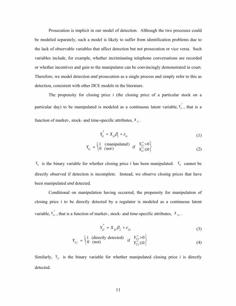
The propensity for closing price i (the closing price of a particular stock on a

particular day) to be manipulated is modeled as a continuous latent variable,

iY

1 , that is a

function of market-, stock- and time-specific attributes, iX

1 .

iiiXY

1111

(1)

0 0

if )not( 0)dmanipulate( 1

1

11 i

ii Y

YY (2)

iY

1 is the binary variable for whether closing price i has been manipulated. iY

1 cannot be

directly observed if detection is incomplete. Instead, we observe closing prices that have

been manipulated and detected.

Conditional on manipulation having occurred, the propensity for manipulation of

closing price i to be directly detected by a regulator is modeled as a continuous latent

variable,

iY

2 , that is a function of market-, stock- and time-specific attributes, iX

2 .

iiiXY

2222

(3)

00

if (not) 0detected)(directly 1

2

22 i

ii Y

YY (4)

Similarly, iY

2 is the binary variable for whether manipulated closing price i is directly

detected.

12

Conditional on manipulation having occurred and not being directly detected, the

propensity for manipulation of closing price i to be indirectly detected is modeled as a

continuous latent variable,

iY

3 , that is a function of market-, stock- and time-specific

attributes, iX

3 .

iiiXY

3333

(5)

00

if (not) 0detected)y (indirectl 1

3

33 i

ii Y

YY (6)

iY

3 is the binary variable for whether the manipulated closing price i is indirectly detected.

< Figure 1 here >

Figure 1 graphically illustrates our three-equation DCE model. A sample of closing

prices falls into two disjoint sets, A and Ac. Set A consists of closing prices that have been

manipulated and either directly or indirectly detected. Set Ac consists of closing prices that

have either not been manipulated or have been manipulated but have evaded both direct and

indirect detection. iY

1 , iY

2 and iY

3 cannot be separately observed. We observe sets A and Ac

in a sample of data and estimate the model’s parameters using maximum likelihood, as in

Poirier (1980) and Feinstein (1990). The details and derivation of the likelihood function are

in Appendix A.

2.4 ALTERNATIVE MODELS

Identification in DCE models is achieved through predictor variables that are

uniquely associated with one stage. That is, variables that predict manipulation but not direct

or indirect detection, variables that predict direct detection but not manipulation or indirect

13

detection and variables that predict indirect detection but not manipulation or direct

detection.7 In order to find such variables we exploit the helpful fact that detection occurs

after manipulation. Variables that are only observed after manipulation can affect the ex-post

probability of detection but not the ex-ante incentives to engage in manipulation and

therefore provide a natural set of variables for identification (a similar approach is used by

Wang (2012)). Distinguishing between direct and indirect detection is more difficult because

we do not have a clear temporal order to exploit. Therefore, we estimate an alternative two-

equation model (similar to the original DCE model used in Feinstein (1989, 1990)) that

allows detection to result from direct or indirect detection but makes no effort to distinguish

between the two. Appendix B contains the equations and likelihood function for this model.

Our DCE model, like the rest of the DCE literature, assumes errors are independently

distributed. In practice, the errors of one process (e.g., manipulation) may be correlated with

the errors of another (e.g., detection), if expectations simultaneity exists and is not

incorporated into the model. For example, regulators may be more likely to investigate

stock-days that have a higher probability of manipulation. We therefore estimate a third

model with expectations simultaneity in which we add the probability of manipulation,

11 iXM , to the right hand side of both detection equations. This model allows the

probability of a regulatory investigation to depend on the probability of manipulation.

Appendix B contains the full set of equations and likelihood function.

3. Variables and Model Specifications

Table II defines the independent variables used in our econometric models. Most

variables primarily influence either manipulation or detection, but have indirect effects on the

other process due to interaction between manipulators and regulators. For example, if fund

managers manipulate closing prices at quarter-ends then a primary determinant of the

7 For a more formal discussion of the identification issue see Feinstein (1990).

14

probability of manipulation is whether or not a day is a quarter-end. A regulator that is aware

of this association is more likely to investigate suspicious trading on quarter-end days and

therefore whether or not a day is a quarter-end is a secondary determinant of the probability

of detecting manipulation. We discuss variables according to their primary association - first

those associated with manipulation, then detection and lastly both manipulation and

detection.

< Table II here >

An order can move prices for at least two reasons: (i) it mechanically moves price

from the bid quote to the ask quote (or vice versa) or beyond the prevailing best quotes by

executing the volume at the best quotes; and (ii) it conveys information and causes revision

of beliefs about the value of the stock. A manipulator can exploit one or both of these

mechanisms to influence prices. The ability to use the first mechanism to manipulate a stock

price depends on the liquidity of the stock, which we measure using market capitalization,

turnover, the Amihud (2002) illiquidity metric (ILLIQ), and bid-ask spread, although at no

stage are all four variables included in a model at the same time. The ability to use the

second mechanism to manipulate a stock price depends on the degree of information

asymmetry, which we measure using the number of analysts’ forecasts of the stock’s earnings

(analyst coverage) and a dummy variable for whether or not the stock is included in a broad

market index. Some closing price manipulation is conducted by company insiders. In

addition to analyst coverage, monitoring by institutional investors may constrain insider

manipulation. We proxy for institutional holdings with the percentage of shares held by

mutual funds.

We also include variables that capture various motivations for manipulation.

Theoretical and empirical evidence suggests that stock prices are manipulated to profit from

options on the underlying stock or from futures contracts on indices, particularly in the period

immediately prior to expiry (e.g., Stoll and Whaley, 1991; Kumar and Seppi, 1992; Jarrow,

15

1994; and Ni et al., 2005). Therefore, we include a dummy variable for whether or not a

stock has listed options and a second dummy variable indicating, for stocks with listed

options, whether it is the last trading day prior to expiry of the options. Fund managers are

known to manipulate closing prices at the end of reporting periods such as the last day of a

month or a quarter (e.g., Carhart et al., 2002; Bernhardt and Davies, 2009; and Ben-David et

al., 2011). Therefore, we include dummy variables for the last trading day in each month and

quarter, and interactions of the dummy variables with the percentage of shares held by mutual

funds. Closing prices are also known to have been manipulated to avoid margin calls and to

maintain a stock’s listing on an exchange with a minimum price requirement. These

incentives for manipulation are triggered when a stock’s price falls to a critical level and

therefore are more likely to occur following declines in a stock’s price. We include a price

trend variable (a stock’s rolling one-month return) to examine these two and other similar

motivations related to price movements. Finally, to investigate manipulation associated with

secondary equity offerings (SEO), we include a dummy variable for one-month periods prior

to each SEO issue. The one-month window is likely to contain the SEO pricing periods,

which is when closing prices might be manipulated.

Volatility is likely to have more than one effect on manipulation. Hillion and

Suominen (2004) suggest that broker execution ability is more valuable when volatility is

higher and therefore high volatility leads to closing price manipulation by brokers that

attempt to alter their customers’ inference about their execution ability. However, volatility

can also deter manipulators if, for example, manipulators perceive volatile stocks as more

likely to attract the regulator’s attention. This could occur due to an extreme day-end

abnormal return or due to an overnight return that creates a return reversal. Further,

idiosyncratic volatility presents a risk to a manipulator because the stock price can move

against them. Our sample of prosecuted instances of manipulation contains cases in which,

despite the manipulator’s intent to increase the price, the day-end return is negative. We

16

measure idiosyncratic volatility using the standard deviation of residuals from a market

model of returns.

The variables associated primarily with detection and prosecution include

government regulatory budget and the number of closing price manipulation prosecutions in

the previous year. Government regulatory budgets, in our case the budgets of the SEC and

the Ontario Securities Commission, determine the amount of resources available to conduct

investigations and prepare cases for prosecution. Therefore, larger regulatory budgets are

likely to be associated with greater capacity to prosecute manipulation.8 The number of

closing price manipulation prosecutions measures the effectiveness and experience of the

regulator in detecting and prosecuting closing price manipulation.

Closing price manipulation is more likely to be directly detected when it causes

abnormal trading characteristics that trigger alerts in automated market surveillance systems.

The measures of abnormal trading characteristics that we use are abnormal day-end return,

order imbalance at the end of the day (the amount of buyer initiated trading in excess of seller

initiated trading), and price reversion (the return from the closing price to the following

morning’s price).9 Manipulation affects these trading characteristics because in attempting to

8 Stock exchanges also have responsibility for manipulation surveillance, so government regulatory budget

only measures part of the total amount spent on regulation and enforcement. Despite this, government

budgets are reasonable proxies for the total enforcement effort because as DeMarzo et al. (2005) illustrate

self-regulatory organizations are likely to take into consideration the level of government-level regulation

and set their enforcement at a level that is just enough to pre-empt government enforcement. A potential

problem with this measure of regulator budget is that it is endogenous, i.e., government regulatory budgets

are increased in times or countries where manipulation is more widespread. The consequence of this

potential endogeneity is to underestimate regulation’s deterrence effect on manipulation.

9 Abnormal day-end trading characteristics can also occur for many reasons other than manipulation, such

as news arrivals at the end of the day. These other causes of abnormal trading do not invalidate its relation

with detection of manipulation because regardless of the cause, abnormal trading that triggers alerts in

17

influence the closing price manipulators typically buy or sell heavily in the last minutes

before the close creating a liquidity imbalance (e.g., Comerton-Forde and Putniņš, 2011b),

which may in turn induce other market participants to trade.10 Given overnight for new

orders to enter the market and resolve the imbalance, prices often revert towards their original

levels the following morning (e.g., Carhart et al., 2002).

Many instances of manipulation, however, do not create the abnormal trading

characteristics that trigger alerts, but can be detected through investigations of other instances

of manipulation or investor complaints. Such indirect detection is more likely if unusual

trading patterns exist in near proximity (e.g., nearby days in the same stock) because the

probability of an alert and subsequent investigation is higher. Therefore, as determinants of

indirect detection, we include measures of abnormal trading aggregated through time in a

particular stock.11 In the two-equation model the direct and indirect detection variables are

combined into a single detection equation, thereby reducing the potential problem of weak

identification of direct and indirect detection.

< Table III here>

market surveillance systems draws the attention of the regulator and therefore increases the probability that

manipulation is detected. Further, manipulation that is accompanied by abnormal trading characteristics

such as price spikes and reversals, are more likely to be prosecuted (a process, which in our model is

combined with detection) because one of the elements in proving manipulation in court is artificiality in

prices or volumes, i.e., a distortion from ‘natural’ market characteristics.

10 Manipulation can also be conducted using quotes to provide misleading signals of intentions to trade.

Such forms of manipulation are also illegal and, if successful, are likely to be associated with similar

characteristics, such as abnormal returns, increased volume and price reversion.

11 We also construct measures of abnormal trading on a particular day aggregated across all stocks on the

corresponding exchange, but find no relation with the probability of indirect detection.

18

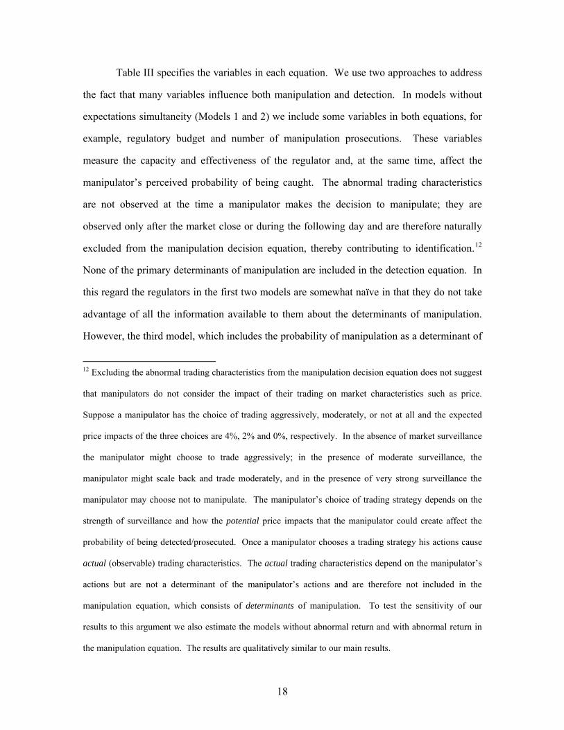
Table III specifies the variables in each equation. We use two approaches to address

the fact that many variables influence both manipulation and detection. In models without

expectations simultaneity (Models 1 and 2) we include some variables in both equations, for

example, regulatory budget and number of manipulation prosecutions. These variables

measure the capacity and effectiveness of the regulator and, at the same time, affect the

manipulator’s perceived probability of being caught. The abnormal trading characteristics

are not observed at the time a manipulator makes the decision to manipulate; they are

observed only after the market close or during the following day and are therefore naturally

excluded from the manipulation decision equation, thereby contributing to identification.12

None of the primary determinants of manipulation are included in the detection equation. In

this regard the regulators in the first two models are somewhat naïve in that they do not take

advantage of all the information available to them about the determinants of manipulation.

However, the third model, which includes the probability of manipulation as a determinant of

12 Excluding the abnormal trading characteristics from the manipulation decision equation does not suggest

that manipulators do not consider the impact of their trading on market characteristics such as price.

Suppose a manipulator has the choice of trading aggressively, moderately, or not at all and the expected

price impacts of the three choices are 4%, 2% and 0%, respectively. In the absence of market surveillance

the manipulator might choose to trade aggressively; in the presence of moderate surveillance, the

manipulator might scale back and trade moderately, and in the presence of very strong surveillance the

manipulator may choose not to manipulate. The manipulator’s choice of trading strategy depends on the

strength of surveillance and how the potential price impacts that the manipulator could create affect the

probability of being detected/prosecuted. Once a manipulator chooses a trading strategy his actions cause

actual (observable) trading characteristics. The actual trading characteristics depend on the manipulator’s

actions but are not a determinant of the manipulator’s actions and are therefore not included in the

manipulation equation, which consists of determinants of manipulation. To test the sensitivity of our

results to this argument we also estimate the models without abnormal return and with abnormal return in

the manipulation equation. The results are qualitatively similar to our main results.

19

the probability of detection, treats regulators as sophisticated in that they are aware of the

probability of manipulation and use this information in their detection processes.

We test the key over-identifying restrictions using likelihood ratio tests as described

by Dhrymes (1994). We use the approach of Kadane (1974) to sequentially test blocks of

exclusion restrictions.13 All of the tests fail to reject the null hypothesis that the exclusion

restriction is valid, thereby supporting the theoretical motivation of our model specification

and the requirements for identification of the models.

4. Data

We construct samples of prosecuted closing price manipulation cases (events) and

stock-days in which no manipulation is detected or prosecuted (non-events) using

endogenous stratified sampling. Due to the rare nature of events, we collect all available

events and only a fraction of non-events.14

We manually collect all of the closing price manipulation cases detected and

prosecuted by market regulators in the US and Canada in the period 1 January 1997 to 1

January 2009. We systematically identify the cases from searches of the litigation releases

and filings of the market regulators SEC, OSC, RS, IDA, MFDA, IIROC, NYSE Reg and

13 Specifically, we test the exclusion of: (i) abnormal trading characteristics from the manipulation equation

(Models 1, 2, 3); (ii) abnormal trading characteristics from the indirect detection equation (Models 1, 3);

(iii) time-series aggregates of abnormal trading characteristics from the manipulation equation (Models 1,

2, 3); (iv) time-series aggregates of abnormal trading characteristics from the direct detection equation

(Models 1, 3); and (v) all of the above exclusions simultaneously.

14 Endogenous stratified sampling is widely used to increase the precision of estimates (Cameron and

Trivedi, 2005) and mitigate potential biases that can result from rare events (King and Zeng, 2001).

20

AMEX DRC15 and searches of the legal databases Lexis, Quicklaw and Westlaw. From the

appendices of SEC annual reports we obtain lists of the case names and filing dates of all the

instances of market manipulation against which the SEC took legal action in the fiscal years

1997 to 2005. We manually examine the litigation releases of each case in these lists to

identify instances of closing price manipulation. For cases in which insufficient details are

provided by the market regulators we obtain court records and filings through the

Administrative Office of the US Courts using the PACER service.

We eliminate cases from our sample if: (i) insufficient information is available to

determine which stocks were manipulated on which days; (ii) the manipulation occurred in an

over-the-counter market; (iii) the manipulated securities were not common stock; (iv) the

manipulation did not involve trade-based techniques; (v) trade and quote data are not

available; or (vi) the manipulated stocks do not have at least three months of trading prior to

the start of manipulation.16 The final sample of detected and prosecuted closing price

manipulation is composed of 184 instances of manipulation with complete data. These 184

instances of a stock manipulated on a particular day are obtained from eight independent

legal cases, each containing multiple instances of closing price manipulation.

The prosecuted instances of closing price manipulation involve 31 stocks from four

exchanges: NYSE, AMEX, TSX and TSX-V. Although we examine litigation releases and

filings between 1997 and 2009, the first and last instances of manipulation in our sample

15 The full names of these regulators are US Securities and Exchange Commission (USA), Ontario

Securities Commission (Canada), Market Regulation Services Inc. (Canada), Investment Dealers

Association (Canada), Mutual Funds Dealers Association (Canada), Investment Industry Regulatory

Organization of Canada (Canada), NYSE Regulation Inc. (USA) and AMEX Division of Regulation and

Compliance (USA), respectively.

16 Although cases in which insufficient information is available to determine the manipulated stock and date

cannot be included in the manipulation sample, they are included in the population count of prosecuted

manipulation. Consequently, these cases affect the estimates via their influence on the observation weights.

21

occur in 1998 and 2005, respectively. The difference between the date of the last examined

litigation release and filing and the date of the last instance of manipulation reflects the

significant amount of time between when an instance of manipulation occurs and when it is

finally prosecuted. The case names, alleged misconduct and legal outcomes are described in

Appendix C. There is considerable variation in the manipulation cases with regard to the

manipulator (e.g., fund manager, corporate insider, broker, shareholder, proprietary trader)

and the motivation for manipulation.

To obtain the sample in which manipulation is not detected and not prosecuted, for

each manipulated stock-day we take all other stock-days on the corresponding exchange in a

period of one month up to and including the manipulation date. After eliminating stock-days

with missing or erroneous data, this sample includes 1,249,748 observations.

We obtain intra-day trade and quote data, expiry dates for listed options, and index

composition data from the Thomson Reuters Tick History database maintained by the

Securities Industry Research Centre of Asia-Pacific (SIRCA). We obtain the remaining data

from Thomson Reuters Datastream, Thomson Reuters Mutual Fund Database, Thomson

Reuters SDC Platinum and the websites of the regulators. We apply normalizing

transformations to the data as documented in Table II.

< Table IV here >

Table IV reports means, standard deviations and medians of the variables for the

sample of prosecuted closing price manipulations and the sample that does not contain

prosecuted manipulation. Ignoring the biases due to incomplete detection for now, the

difference in means and medians between the two samples is consistent with our expectations

for most variables. The sample of detected and prosecuted manipulation involves less liquid

stocks (lower market capitalization, turnover, larger spreads and higher ILLIQ), lower levels

of institutional following (less analyst forecasts, index constituency and mutual fund

22

holdings), and lower idiosyncratic volatility. Manipulation is more concentrated on month-

end and quarter-end days, as well as one-month periods prior to secondary equity offerings.

The detected manipulation sample is also associated with lower government regulatory

budgets, higher abnormal returns, greater price reversion and larger positive order

imbalances, as well as higher aggregate levels of the abnormal trading variables on other days

in the same stock.

5. Results

First we present the estimated model coefficients and discuss the determinants of

manipulation and detection. Next, we use our models to estimate the frequency of

manipulation and detection. Finally, we report results of robustness tests.

5.1 THE DETERMINANTS OF MANIPULATION AND DETECTION

We use two approaches to select variables for the final models from the large number

of potential variables and alternative measures (e.g., the several proxies for liquidity). In the

first approach we include all of the variables suggested by theory (as specified in Table III),

then remove insignificant variables and re-estimate the models. The second approach is a

forward stepwise variable selection procedure.17 Both approaches give similar sets of

variables so we only report the results from the first procedure. For robustness we also

estimate models with alternative sets of variables including those not deemed to be

significant by the stepwise procedure. 17 Starting with just the constant terms, in each iteration we add variables that result in the largest increase

in log-likelihood and re-estimate the model. This is repeated until additional variables do not yield a

significant improvement in the log-likelihood. The stepwise variable selection procedures result in a

relatively large proportion of statistically significant coefficients because highly statistically insignificant

variables are not included in the final specifications.

23

Table V reports the coefficient estimates and marginal effects (in parentheses).18 For

continuous variables, the marginal effects measure the percentage change in the probability

of either manipulation, direct or indirect detection for a one percent change in the value of the

independent variable. The statistical significance of results in Table V assumes observations

are independent. Because the 184 instances of prosecuted manipulation in our sample are

related to eight legal cases, the level of statistical significance reported in Table V is likely to

be inflated. Therefore, we place more emphasis on the economic significance of the

magnitudes. In robustness tests we apply a block-bootstrap procedure (to a subset of the

sample due to computational constraints) that accounts for the relations between instances of

prosecuted manipulation. These tests suggest that although statistical significance in Table V

may be inflated most variables in our model are statistically significant.

< Table V here >

We find that government regulatory budget has a strong effect on both manipulation

and detection. Across all three models larger government regulatory budgets increase the

probability of detecting and prosecuting manipulation and also decrease the probability of

manipulation. The latter effect is likely to be because increased regulatory capacity has a

deterrence effect on manipulation. This is consistent with the conclusions made by Pirrong

(1995) based on a historical overview of manipulation under various regulatory regimes. We

estimate that a 1% increase in a government regulator’s real budget per stock results in a

18 Marginal effects are calculated as 2)1(

PrX

X

e

e

X

, where: Pr is the estimated probability of

manipulation, direct detection and indirect detection;

are the coefficient estimates; and X are the

observed variable values. They are reported as a percentage of Pr. Marginal effects are calculated for each

observation and then averaged over the entire sample.

24

2.0% decrease in the amount of closing price manipulation and a 1.5% increase in the rate of

prosecution.19 Because our models include dummy variables for each of the markets, the

effect of budget on manipulation and detection is identified primarily through its time series

variation.20 The Pearson correlation coefficients between real per-stock government

regulatory budget and the number of closing price manipulation prosecutions filed by the

regulator in a rolling one-year window are 0.81 and 0.47 in the US and Canada, respectively.

This further illustrates the strong association between regulatory budgets and the probability

of detection. Real per-stock regulatory budgets in both the US and Canada have steadily

increased during the past decade, increasing the probability of detection and putting

downward pressure on the rate of manipulation.

The coefficients of the number of analyst forecasts and the index constituency

dummy suggest that stocks with greater information asymmetry are more likely to be

manipulated. A 20% reduction in the number of analysts’ forecasts is estimated to increase

the probability of manipulation by approximately 4%. This finding holds across all three

models and the two information asymmetry variables make the largest contribution to

maximizing the model likelihood. This result is consistent with theory (e.g., Allen and Gale,

1992; Kumar and Seppi, 1992; and Aggarwal and Wu, 2006): information asymmetry makes

it difficult for market participants to identify whether an aggressive buyer is an informed

trader or a manipulator.

Analysts, together with institutional investors, may constrain manipulation by

corporate insiders through stronger monitoring of insiders’ actions. Consistent with this

19 The former estimate is the average marginal effect across the three models and the later is from Model 2.

Because Model 2 aggregates direct and indirect detection, it provides a single estimate for the effect of

budget on the total amount of detection (direct and indirect). Models 1 and 3 provide separate estimates for

the effect of budget on direct and indirect detection.

20 There is significant time series variation in regulator budgets. In both the US and Canada the maximum

value of real budget per stock is more than twice the minimum.

25

explanation, in addition to the negative relation between analyst coverage and manipulation,

we also find a negative relation between mutual fund ownership and the propensity for

manipulation. A one standard deviation increase from the average mutual fund ownership (as

a percentage of shares outstanding) is associated with an expected 9% decrease in the

probability of manipulation.

The coefficients of the liquidity and illiquidity variables, market capitalization and

ILLIQ, are positive and negative, respectively.21 The interpretation of this result is not

straightforward. The liquidity variables are correlated with the asymmetric information

proxies. Therefore, highly liquid stocks, which also tend to have low information

asymmetry, are given a low probability of manipulation by the information asymmetry

variables. The positive (negative) coefficient of the liquidity (illiquidity) variable therefore

suggests that manipulators do not favor the most illiquid stocks. Taken together, the

information asymmetry and liquidity coefficients suggest that manipulators generally prefer

stocks that are at neither end of the liquidity spectrum. To confirm this interpretation we re-

estimate the models replacing the continuous liquidity variables with quintile dummy

variables. We find that the probability of manipulation is highest for stocks in the third and

fourth quintiles where the first quintile is defined as having the highest liquidity. We

conclude that manipulators favor stocks with mid to low levels of liquidity.

A likely explanation of the previous result is that highly liquid stocks are difficult to

manipulate because of the high levels of trading activity, substantial order book depth and

low information asymmetry. Very illiquid stocks tend not to be favored by manipulators

because they generally lack the incentives or magnitude of potential profits that mid-range

and highly liquid stocks have. For example, fund managers, in general, hold relatively liquid

stocks and any illiquid stocks they may hold only represent a small proportion of their

portfolios. Therefore, manipulating the closing prices of very illiquid stocks is unlikely to

give fund managers much benefit in overstating their portfolio’s performance. Similarly,

21 Using spread as an alternative measure of liquidity produces similar results.

26

derivatives are less frequently available on very illiquid stocks and such stocks are typically

not constituents of major indices. Finally, brokers are more likely to manipulate stocks for

the purpose of altering their clients’ inference of their execution ability when the clients and

orders are large. This seldom occurs in very illiquid stocks.

The results in Table V also indicate that stocks are significantly more likely to be

manipulated on month-end and quarter-end days. Carhart et al. (2002) present evidence that

stock price manipulation on month-end and quarter-end days is largely attributable to fund

managers. Consistent with this explanation, the coefficients of the interaction terms

involving month/quarter-end dummy variables and fund holdings are positive and statistically

significant indicating that a high proportion of mutual fund ownership increases the

likelihood that a stock is manipulated at month/quarter end. Therefore, our results suggest

that fund managers are associated with a significant proportion of all manipulation.

On the other hand, the listed options dummy variables are not statistically significant

in our model. Because options tend to be listed on relatively liquid stocks, we do not rule out

the possibility that options do affect manipulation but that this effect is overshadowed by the

liquidity variables. Whether a stock’s price has been increasing or decreasing over the prior

month does not have a significant effect on the likelihood of manipulation. Similarly we do

not find statistical evidence of a relationship between secondary equity offerings and closing

price manipulation.

All else equal, idiosyncratic volatility reduces the likelihood of manipulation. A 20%

increase in the standard deviation of daily return residuals is estimated to decrease the

probability of manipulation by 9%. Because idiosyncratic volatility is negatively correlated

with liquidity, it is important to note that this estimate is the expected effect when holding

liquidity constant.22 This finding is consistent with the explanation that idiosyncratic

22 The correlation between idiosyncratic volatility and the liquidity proxies (market capitalization and

turnover) is between -0.43 and -0.50. The correlation between idiosyncratic volatility and the illiquidity

proxies (bid-ask spread and ILLIQ) is between 0.51 and 0.71.

27

volatility deters manipulation because it increases the probability of an alert and subsequent

regulatory investigation. The negative relation could also be because, all else equal, stocks

with high idiosyncratic volatility increase the risk to the manipulator that the stock price will

move against them.

Turning to the variables that affect detection, in all three models the abnormal trading

characteristics (abnormal return, reversion and order imbalance) increase the probability of

direct detection. The type of market closing mechanism is likely to affect the timing of

manipulation-induced abnormal trading characteristics. We therefore examine various day-

end windows (60, 30, 10 and 5 minutes before the close) and find that the results are

consistent across the alternative lengths.23

Indirect detection of manipulation in a particular stock-day is more likely when there

is abnormal trading in that stock during a period of a few days either side of that day. In

particular, an instance of manipulation that is accompanied by a number of abnormal day-end

returns and overnight price reversions in a period of two weeks has an increased probability

of being indirectly detected. The regulator notices the abnormal patterns in returns and upon

investigation reveals instances of manipulation that did not trigger alerts in surveillance

23 In our sample the Canadian exchanges, TSX and TSX-V, have simple closing mechanisms: trade occurs

continuously until 4:00pm at which time the market closes and the closing price is the price of the last

trade. The TSX introduced a closing call auction for some stocks, with a staggered implementation from

March 2004. This does not affect any of the observations in our sample because there are no prosecuted

manipulation cases on the TSX after the introduction of the closing call auction. The TSX-V introduced a

closing call auction for some stocks from December 2011, after the end of our sample period. The closing

mechanisms on the NYSE and AMEX allow orders to be specified for execution at the closing price and

the specialists intervene in setting closing prices. Although the NYSE and AMEX closing procedures are

sometimes described as auctions, they bear little resemblance to any other auction procedure (Hasbrouck,

2007), particularly automated closing call auctions, such as the ones currently used at Euronext Paris and

the London Stock Exchange, for example.

28

systems. Combining direct and indirect detection into a single detection process, as in the

two-equation model, produces similar results regarding the effect of the abnormal trading

characteristics on the probability of detection.

The results from Model 3 suggest that ceteris paribus, i.e., after controlling for things

such as the effect of abnormal trading characteristics on detection, the probability of detection

increases as the probability of manipulation increases. A positive relation suggests that

regulators are aware of factors that influence the probability of manipulation and that they use

this knowledge in detecting, investigating and prosecuting manipulation. Adding the

expectation simultaneity term in Model 3 does not substantially change the conclusions about

the other determinants of manipulation and detection.

The exchange dummy variables are included in all equations to allow for different

levels of manipulation and detection in each of the two countries (US and Canada) or in

different exchanges within a country. Industry dummy variables on the other hand are not

included in the final models as they are generally not statistically significant. The pseudo R2

of the models, based on McFadden’s likelihood ratio (one minus the ratio of the log-

likelihood with all predictors and the log-likelihood with intercepts only) range from 0.17 to

0.23.

5.2 THE FREQUENCY OF MANIPULATION AND DETECTION

The three models of manipulation and detection allow estimation of the underlying

rate of manipulation (detected and not detected) and the fraction of manipulation that remains

undetected. Denoting the parameter estimates by *

1 ,

*

2 and

*

3 , applying Bayes’s law for

the three-equation models gives the probability of an undetected manipulated closing price in

the sample with no detected or prosecuted manipulation (set Ac) as:

29

*33

*22

1*11

*22

*11

1

*33

*22

*22

1*11

03

,02

|11

Pr

iXI

iXD

iXM

iXD

iXM

iXI

iXD

iXD

iXM

iY

iY

iY

(7)

where M( ), D( ) and I( ) are defined in Appendix A as the probabilities for manipulation,

direct detection and indirect detection, respectively. For the two-equation model the

probability of an undetected manipulated closing price in set Ac is:

*22

*11

1

*22

1*11

02

|11

Pr

iXD

iXM

iXD

iXM

iY

iY

(8)

These estimates of the probability of manipulation (given that manipulation has not

been prosecuted) are useful in efficiently allocating regulators’ resources, particularly when

resources are increased and it becomes possible to investigate additional cases of suspected

manipulation. These probability estimates can also be used to study the characteristics of

undetected or not prosecuted closing price manipulation.

Using a similar approach to Feinstein (1990), the fraction of undetected manipulation

in the population can be consistently estimated as:

cAiiii YYY

Tn

N0,0|1Pr 321 (9)

where T is the total number of observations in the population (the sum of the number of

observations in sets A and Ac), N is the population number of observations in set Ac and n is

the sample number of observations in set Ac.

Models 1 and 2 estimate the fraction of undetected closing price manipulation in the

population as 1.14% and 1.08% of all stock-days, respectively. The rate of detected and

prosecuted manipulation in the population (number of observations in set A divided by T) is

0.004%. This suggests that there are many more instances of manipulation not prosecuted

than there are prosecuted manipulations. In fact, these estimates suggest that only about

0.4% of all manipulation is prosecuted. For every prosecuted closing price manipulation

approximately 308 to 326 manipulations remain either undetected or not prosecuted. Here

30

the limitation of modeling detection and prosecution together becomes clear – we cannot

infer the fraction of the not prosecuted manipulation that was detected. Adding the rates of

prosecuted and not prosecuted manipulation, the underlying rate of manipulation in the

population is estimated at 1.14% to 1.08% of stock-days. This is not significantly different

from the rate of manipulation that is not prosecuted, because only a small fraction of

manipulation is prosecuted.

What explains the large difference between the total amount of manipulation and the

amount of prosecuted manipulation? We believe there are two main factors. First,

discussions with regulators and other anecdotal evidence indicate that a significant proportion

of the manipulation detected by regulators is not prosecuted. One of the main reasons for this

is difficulty in obtaining sufficiently incriminating evidence. Given that many non-

manipulative motivations for trading can lead to the same pattern of trades and market impact

as manipulation, what distinguishes manipulative from non-manipulative trading is

manipulative intent (see, for example, Ledgerwood and Carpenter, 2012). In practice,

proving manipulative intent often requires recorded telephone conversations or intercepted

emails, which contain explicit statements of the manipulator’s intent. In place of formal legal

action, in some instances regulators with insufficient evidence simply warn the suspected

manipulators about their suspicious trading patterns, thereby hoping to stop further

manipulation. As DeMarzo et al. (1998) point out, optimal enforcement must balance the

benefits of enforcement against the costs, which in practice can be substantial, and therefore

it is often optimal to pursue only a fraction of the possible cases.

Second, many instances of manipulation are very difficult to detect. Given the

significant penalties for convicted manipulation (criminal charges) it is reasonable to expect

that manipulators will only choose to do so when the probability of detection and prosecution

is low. To reduce the probability of detection manipulators scale back the aggressiveness of

their trading and alter the timing of their trades to conceal their actions from the regulator

(Comerton-Forde and Putniņš, 2011b). Consistent with this explanation we find that: (i)

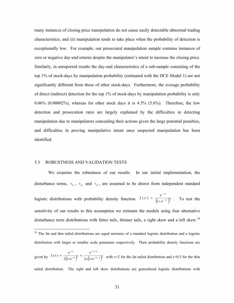
31

many instances of closing price manipulation do not cause easily detectable abnormal trading

characteristics; and (ii) manipulation tends to take place when the probability of detection is

exceptionally low. For example, our prosecuted manipulation sample contains instances of

zero or negative day-end returns despite the manipulator’s intent to increase the closing price.

Similarly, in unreported results the day-end characteristics of a sub-sample consisting of the

top 1% of stock-days by manipulation probability (estimated with the DCE Model 1) are not

significantly different from those of other stock-days. Furthermore, the average probability

of direct (indirect) detection for the top 1% of stock-days by manipulation probability is only

0.06% (0.00002%), whereas for other stock days it is 4.5% (5.6%). Therefore, the low

detection and prosecution rates are largely explained by the difficulties in detecting

manipulation due to manipulators concealing their actions given the large potential penalties,

and difficulties in proving manipulative intent once suspected manipulation has been

identified.

5.3 ROBUSTNESS AND VALIDATION TESTS

We examine the robustness of our results. In our initial implementation, the

disturbance terms, i1 , i2

and i3 , are assumed to be drawn from independent standard

logistic distributions with probability density function 21)(

e

ef . To test the

sensitivity of our results to this assumption we estimate the models using four alternative

disturbance term distributions with fatter tails, thinner tails, a right skew and a left skew.24

24 The fat and thin tailed distributions are equal mixtures of a standard logistic distribution and a logistic

distribution with larger or smaller scale parameter respectively. Their probability density functions are

given by 2/

/

21212

)(s

s

es

e

e

ef

with s=2 for the fat tailed distribution and s=0.5 for the thin

tailed distribution. The right and left skew distributions are generalized logistic distributions with

32

The marginal effects of most independent variables are very similar under the different

disturbance term distributions, suggesting the results are not overly sensitive to the assumed

disturbance term distribution.

The statistical significance of our main results may be affected by dependencies

between observations causing clustering of errors. This can occur due to manipulators

targeting particular stocks or days multiple times, or due to our 184 instances of prosecuted

manipulation being related to eight legal cases. To address this concern we implement two

versions of the bootstrap algorithm described in Cameron et al. (2011): (i) clustering standard

errors by stock and by date (double clustering); and (ii) clustering standard errors by legal

case. The first version provides consistent standard errors under arbitrary two-way error

clustering within stocks and dates and the second accounts for relations between observations

related to the same legal case. We run 500 repetitions of each bootstrap estimation. Due to

computational constraints we use a sample consisting of all of the detected manipulation

observations and randomly selected 1% of the stock-days with no detected manipulation,

adjusting observation weights accordingly.

Nonlinear maximum likelihood estimators can be biased in finite samples. Although

our total sample size is large, the number of manipulation and detection observations is

relatively small due to the rare nature of these events.25 We examine the potential influence

of finite-sample biases by estimating the bootstrap bias-corrected parameter estimates

suggested by Efron and Tibsharani (1993) and Cameron and Trivedi (2005). The difference

probability density )1(1

)(

b

e

bef

and b=2 for the right skew distribution and b=0.5 for the left skew

distribution.

25 King and Zeng (2001) document a special case of the finite sample bias for rare events in logistic

regression. However, their results are not directly applicable to DCE models consisting of multiple

simultaneous equations.

33

between the bias-corrected estimates and uncorrected estimates allow us to gauge the

magnitude of the potential bias.

< Table VI here >

Table VI reports the results of the bootstrap-based corrections for double-clustered

errors and finite-sample bias. The coefficient and marginal effect estimates using the reduced

size sample are similar to those estimated using the full sample. Despite the fact that the

cluster-robust standard errors are larger on average, most coefficients remain statistically

significant at the 1% level. Similarly, the statistical significance when standard errors are

clustered by legal case (results available upon request) is lower, but most of the variables

remain statistically significant. The bias-corrected estimates are similar to those without

correction, suggesting finite-sample bias does not have a large influence on our estimates.

We also examine the robustness of our results to changes in the sample composition,

the time period from which the sample is drawn, different model specifications and

alternative variable definitions. To test the sensitivity to the particular sample and time

period we split our data into two sub-samples, first by time (earliest half of the data and latest

half of the data) and then randomly, and estimate the model separately on each sub-sample.

We also re-estimate our model using only post-decimalization data. We test alternative

model specifications by including the variables from Table II that are left out of the reported

models. We examine the sensitivity of the results to the way the variables are measured by

replacing variables with their alternative definitions given in Table II. We find that the main

results hold in each of these robustness tests and therefore we do not report these results.

We conduct three simple validity tests of the main econometric model’s predictions.

First, we expect manipulation to cluster on particular days and in particular stocks that are

manipulated repeatedly. Using the top 1% of predicted manipulation probabilities as a proxy

for manipulated closing prices we examine the distribution of predicted manipulation across

stocks and dates. The distribution is far from uniform with pronounced clustering in

34

particular stocks and on particular dates, as expected. This result holds even after excluding

month-end and quarter-end days. Second, we examine whether the model predicts

manipulation in the lead up to prosecuted instances using a probit regression with prosecuted

manipulation as the dependent variable and a dummy variable for whether the model predicts

manipulation in a rolling window containing the past week as the independent variable. We

obtain a positive and statistically significant coefficient on the independent variable

suggesting the model predicts manipulation in the week leading up to prosecuted instances of

manipulation.

The third test is a form of leave-one-out cross-validation of out-of-sample predictive

accuracy. For each of the eight legal cases in turn we: (i) remove the case (and corresponding

non-manipulated stock-days) from the sample; (ii) estimate the main DCE model (Model 1)

on the remaining data; and (iii) use the model estimates to calculate for each closing price in

the left out data the predicted probability that the closing price falls into the set of prosecuted

manipulations (the probability that the closing price is manipulated and either directly or

indirectly detected). We examine the accuracy of the predicted probabilities using Receiver

Operating Characteristics (ROC) analysis. The Area Under the ROC curve (AUROC)

measures the probability of correct prediction, independent of prior probabilities and

classification thresholds. Hosmer and Lemeshow (2000) suggest the following interpretation

of AUROC values: around 0.5 implies the model performs no better than chance; 0.7-0.8

implies acceptable classification performance; 0.8-0.9 implies excellent performance; and

0.9-1.0 implies outstanding performance (rare). For our main model the out-of-sample

AUROC point estimate is 0.902, with a 95% confidence interval 0.870 to 0.934. These

results suggest our DCE model has excellent out-of-sample classification accuracy,

supporting the validity of the model.

35

6. Conclusions

We examine the determinants of manipulation and its detection using methods that

recognize that only a non-random subset of manipulation is detected and prosecuted. Stocks

with high levels of information asymmetry and mid to low levels of liquidity are most likely

to be manipulated. The probability of manipulation is higher on month-end and quarter-end

days, particularly for stocks with relatively high levels of mutual fund ownership, suggesting

fund managers account for a significant proportion of manipulation. All else equal,

manipulators dislike stocks with high levels of idiosyncratic volatility, possibly because of

the risk that the stock will move against them or due to the increased likelihood of the stock

triggering alerts and attracting the attention of a regulator. Larger government regulatory

budgets increase the rate of prosecution and significantly deter manipulation. These insights

help understand the underpinnings of closing price manipulation and allow regulatory effort

to be focused where manipulation is most likely to occur.

We also find that only a small fraction of manipulation is detected and prosecuted.

For each instance of prosecuted closing price manipulation we estimate that approximately

308 to 326 instances of manipulation remain undetected or not prosecuted. The amount of

manipulation can be reduced by allocating additional resources to regulation. The results

suggest that a 1% increase in government regulatory budgets would result in an estimated

2.0% decrease in the amount of closing price manipulation and a 1.5% increase in the rate of

prosecution. These estimates should be taken into account by policymakers when deciding

on how much resources to allocate to regulation because as pointed out by DeMarzo et al.

(1998) the socially optimal amount of enforcement depends on the frequency of violations

and how violators, in our case manipulators, respond to increased enforcement.

All statistical methods are subject to some degree of estimation error and more

difficult to quantify model error. The statistical method used in this paper is no exception.

Analogous to the way practitioners estimate the value of a company by using multiple

36

methods and taking the average or a range from the various estimates, we hope that future

research will use alternative methods to estimate the prevalence of closing price

manipulation, its determinants and how it responds to regulation. Estimates from alternative

methods will help reduce the uncertainty about model error and therefore increase confidence

in the estimates. As highlighted by this paper, it is important that methods explicitly address

the problem of incomplete detection in order to avoid potentially significant biases in

inference.

In future work it would be useful to extend the sample in time (the last instance of

manipulation in our sample occurs in 2005, reflecting the time taken to bring cases to

prosecution). This would allow examination of how manipulation and detection have

responded to several interesting market structure and regulatory changes, such as the

introduction of a closing call auction for some stocks on the TSX and TSX-V, Regulation

NMS for the US exchanges, and the tendency for surveillance and enforcement roles to shift

from self-regulatory organizations such as stock exchanges to more centralized government-

level regulators. Finally, this study provides an instrument to calculate the probability of

manipulation that has not been prosecuted. This instrument can be used to study the

characteristics of undetected manipulation and refine alerting parameters of market

surveillance systems.

37

Appendix A: Details of Model Estimation Procedure

We define M( ), D( ) and I( ) to be monotonic link functions that link 11

iX , 22

i

X

and 33

iX , to latent probabilities for manipulation, direct detection and indirect detection,

respectively.26 That is,

1Pr 111 ii YXM (A.1)

1|1Pr 1222 iii YYXD (A.2)

0,1|1Pr 21333 iiii YYYXI (A.3)

Table A.I reports the probabilities of an observation (closing price) arriving at various

joint outcomes (represented by cells in the table) of the manipulation and detection processes.

The joint outcomes are mutually exclusive and exhaustive, so the probabilities in Table A.I

sum to one.

Table A.I. Modified detection controlled estimation model probabilities This table reports the probabilities of an observation (a closing price) arriving at various outcomes. M( ) is the probability that a closing price is manipulated. D( ) is the probability that a manipulated closing price is directly detected. I( ) is the probability that a manipulated closing price is indirectly detected, given that it is not directly detected.

Manipulation

Manipulated Not manipulated

Directly detected M( )D( ) 0

Indirectly detected M( )[1 – D( )]I( ) 0 Detection

Not detected M( )[1 – D( )][1 – I( )] 1 – M( )

In order to observe a detected manipulated closing price, the closing price must have

been manipulated and either directly or indirectly detected. These outcomes correspond to

26 In our implementation of this model the link functions are cumulative logistic distribution functions, that

is, 1111 1

1

iXi eXM

, 2222 1

1

iXi eXD

and 3333 1

1

iXi eXI

. The disturbance terms, i1 , i2

and i3 , are from independent logistic distributions with mean zero and variance 3

2 (scale parameter of

one). In robustness tests we examine alternative distributions for the disturbance term.

38

the first two probability rows in Table A.I due to the simplifying assumption of no false

detection.27 Therefore, the log-likelihood of the set of detected manipulated closing prices

(set A), is:

Ai

iiiiiAXIXDXMXDXML 3322112211 1loglog (A.4)

Similarly, for a closing price in which manipulation has not been detected, either: (i)

manipulation has not occurred; or (ii) manipulation has occurred and evaded both direct and

indirect detection. These outcomes correspond to third probability row in Table A.I.

Therefore, the log-likelihood of the set of observations in which manipulation is not detected

(set Ac):

cAi

iiiicAXIXDXMXML 33221111 111loglog (A.5)

The log-likelihood of the full sample is the sum of the log-likelihoods of the two sets of

observations. To estimate this model with data collected from endogenous stratified

sampling (choice-based sampling) we add weights to the observations and the resulting

weighted maximum-likelihood estimator (due to Manski and Lerman (1977)) becomes:

cAiiiiicA

AiiiiiiA

XIXDXMXMw

XIXDXMXDXMwL

33221111

3322112211

111log

1loglog

(A.6)

where swA

/ , )1/()1( sw cA and and s are the fractions of stock-days with

prosecuted manipulation in the population and sample respectively. Note this weighted

estimator does not require knowledge of the underlying rates of manipulation and detection;

it merely accounts for the fact that we sample a different proportion of the observations in the

observable sets A and Ac.

27 More precisely, we assume that the probability of detecting and prosecuting manipulation given that

manipulation has not occurred is zero. This assumption seems reasonable considering the strength of

evidence required to prosecute closing price manipulators.

39

Appendix B: Alternative Models

B.1 TWO-EQUATION (STANDARD DCE) MODEL OF MANIPULATION AND

DETECTION

Using the same notation as for the three-equation model and omitting much of the

explanation the two-equation model of manipulation and detection is as follows.

iiiXY

1111

(B.1)

00

if (not) 0ed)(manipulat 1

1

11 i

ii Y

YY (B.2)

iiiXY

2222

(B.3)

00

if (not) 0(detected) 1

2

22 i

ii Y

YY (B.4)

1Pr 111 ii YXM (B.5)

1|1Pr 1222 iii YYXD (B.6)

Ai

iiAXDXML 2211loglog (B.7)

cAi

iiicAXDXMXML 221111 11loglog (B.8)

cAi

iiicAAi

iiAXDXMXMwXDXMwL 2211112211 11logloglog (B.9)

B.2 THREE-EQUATION MODEL OF MANIPULTION AND DETECTION WITH EXPECTATIONS SIMULTANEITY

iiiXY

1111

(B.10)

00

if (not) 0ed)(manipulat 1

1

11 i

ii Y

YY (B.11)

1Pr 111 ii YXM (B.12)

iiii

XMXY2211222

(B.13)

40

00

if (not) 0detected)(directly 1

2

22 i

ii Y

YY (B.14)

1|1Pr, 1221122 iiii YYXMXD (B.15)

iiii

XMXY3311333

(B.16)

00

if (not) 0detected)y (indirectl 1

3

33 i

ii Y

YY (B.17)

0,1|1Pr, 21331133 iiiii YYYXMXI (B.18)

Representing 11 iXM by M ,

21122 , ii XMXD by D and 31133 , ii XMXI

by I :

Ai

AIDMMDL 1loglog (B.19)

cAi

cAIDMML 111loglog (B.20)

cAi

cAAi

AIDMMwIDMMDwL 111log1loglog

(B.21)

Appendix C: Summary of Manipulation Cases

Case Period of manipulation

Exchange Alleged misconduct Outcomes

SEC v. Competitive Technologies, Inc. et al., Civil Action No. 304 CV 1331 JCH (District of Connecticut)

1-Jul-98 to

29-Jun-01

AMEX A prolonged multi-faceted scheme carried out by several brokers, former brokers and company CEO in an attempt for the manipulators to enrich themselves and avoid margin calls.

Conviction by a federal jury and settlements.

In the Matter of RT Capital Management Inc. et al.

30-Oct-98 to

31-Mar-99

TSX Closing price manipulation of several stocks by several fund managers at the ends of reporting periods to inflate reported performance. This enabled the fund to collect more management fees and earned the fund managers greater remuneration.

Settlement, fines and suspensions.

In the Matter of Spear, Leeds & Kellogg, L.P., Administrative Proceeding File No. 3-11189 / In the Matter of Baron Capital Inc. et al., Administrative Proceeding File No. 3-11096

18-Oct-99 to

1-Nov-99

NYSE Closing price manipulation by a substantial shareholder during the pricing-period for a company acquisition.

Settlement and fines.

In the Matter of John Andrew Scott (OOS 2003-010) / In the Matter of Linda Grace Malinowski (OOS 2003-011) / In the Matter of Matthew Philip Linden (OOS 2003-012)

2-Feb-00 to

4-Jul-00

TSX Manipulation of closing prices over a period of consecutive days in relation to an application for price protection.

Settlements, fines and suspensions.

In the Matter of Douglas Christie (OOS 2002-002)

28-Feb-01 to

29-Jun-01

TSX Manipulation of closing prices over a period of time to increase personal remuneration, which was paid by the trading firm based on market value of the trader’s inventory balance.

Settlement and fines.

In the Matter of Schultz Investment Advisors, Inc. and Scott Schultz, Administrative Proceeding File No. 3-12136

28-Jun-02 to

31-Dec-03

NYSE Closing price manipulation by a fund manager at the ends of reporting periods. This was done to inflate reported performance and subsequently collect more management fees.

Settlement, fine and suspension.

In the Matter of Alfred Simon Gregorian (DN 2006-003) / In the Matter of Research Capital Corporation (DN 2006-005)

12-Nov-03 to

24-Dec-03

TSX-V Manipulation of the closing prices of a single stock over a period of time to create a misleading appearance of strength and stability in the market for the company’s shares.

Settlement, fines and suspensions.

In the Matter of Luc St Pierre (IIROC No. 11)

1-Oct-04 to

30-Sep-05

TSX-V Manipulation of the closing prices of two stocks over a period of time on behalf of anonymous sophisticated investors and a company director.

Conviction by a Disciplinary Panel, fines and suspension.

42

References

Aggarwal, R.K., and Wu, G. (2006) Stock market manipulations, Journal of Business 79,

1915-1953.

Allen, F., and Gale, D. (1992) Stock-price manipulation, The Review of Financial Studies 5,

503-529.

Allen, F., Litov, L., and Mei, J. (2006) Large investors, price manipulation, and limits to

arbitrage: An anatomy of market corners, Review of Finance 10, 645-693.

Amihud, Y. (2002) Illiquidity and stock returns: Cross-section and time-series effects,

Journal of Financial Markets 5, 31-56.

Ben-David, I., Franzoni, F., Landier, A., and Moussawi, R. (2011) Do hedge funds

manipulate stock prices?, Unpublished working paper, Fisher College of Business.

Bernhardt, D., and Davies, R.J. (2005) Painting the tape: Aggregate evidence, Economics

Letters 89, 306-311.

Bernhardt, D., and Davies, R.J. (2009) Smart fund managers? Stupid money?, Canadian

Journal of Economics 42, 719-748.

Cameron, A.C., Gelbach, J.B., and Miller, D.L. (2011) Robust inference with multiway

clustering, Journal of Business and Economics Statistics 29, 238-249.

Cameron, A.C., and Trivedi, P.K. (2005) Microeconomics: Methods and Applications,

Cambridge University Press, New York.

Carhart, M., Kaniel, R., Musto, D., and Reed, A. (2002) Leaning for the tape: Evidence of

gaming behavior in equity mutual funds, Journal of Finance 57, 661-693.

Comerton-Forde, C., and Putniņš, T.J. (2011a) Measuring closing price manipulation, Journal

of Financial Intermediation 20, 135-158.

43

Comerton-Forde, C., and Putniņš, T.J. (2011b) Pricing accuracy, liquidity and trader behavior

with closing price manipulation, Experimental Economics 14, 110-131.

Cumming, D., Johan, S., and Li, D. (2011) Exchange trading rules and stock market liquidity,

Journal of Financial Economics 99, 651-671.

DeMarzo, P.M., Fishman, M.J., and Hagerty, K.M. (1998) Optimal enforcement of insider

trading regulations, Journal of Political Economy 106, 602-632.

DeMarzo, P.M., Fishman, M.J., and Hagerty, K.M. (2005) Self-regulation and government

oversight, Review of Economic Studies 72, 687-706.

Dhrymes, P.J. (1994) Topics in advanced econometrics, Volume II: Linear and nonlinear

simultaneous equations, Springer-Verlag, New York.

Efron, B., and Tibsharani, J. (1993) An introduction to the bootstrap, Chapman and Hall,

London.

Feinstein, J.S. (1989) The safety regulation of U.S. nuclear power plants: Violations,

inspections, and abnormal occurrences, The Journal of Political Economy 97, 115-154.

Feinstein, J.S. (1990) Detection controlled estimation, Journal of Law and Economics 33,

233-276.

Feinstein, J.S. (1991) An econometric analysis of income tax evasion and its detection, Rand

Journal of Economics 22, 14-35.

Fischel D., and Ross, D. (1991) Should the law prohibit manipulation in financial markets?,

Harvard Law Review 105, 503-553.

Goetzmann, W., Ingersoll, J., Spiegel, M., and Welch, I. (2007) Portfolio performance

manipulation and manipulation-proof performance measures, Review of Financial

Studies 20, 1503-1546.

Hasbrouck, J. (2007) Empirical market microstructure: The institutions, economics and

econometrics of securities trading, Oxford University Press, Oxford.

44

Hillion, P., and Suominen, M. (2004) The manipulation of closing prices, Journal of

Financial Markets 7, 351-375.

Hosmer, D.W., and Lemeshow, S. (2000) Applied logistic regression, 2nd Edition, John Wiley

and Sons, New York.

IOSCO (2000) Investigating and prosecuting market manipulation, Technical Committee of

the International Organization of Securities Commissions.

Jarrow, R.A. (1994) Derivative security markets, market manipulation, and option pricing

theory, The Journal of Financial and Quantitative Analysis 29, 241-261.

Jegadeesh, N. (1993) Treasury auction bids and the Salomon squeeze, Journal of Finance 48,

1403-1419.

Jiang, G., Mahoney, P., and Mei, J. (2005) Market manipulation: A comprehensive study of

stock pools, Journal of Financial Economics 77, 147-170.

Jordan, B., and Jordan, S. (1996) Salomon Brothers and the May 1991 Treasury auction:

Analysis of a market corner, Journal of Banking and Finance 20, 25-40.

Kadane, J.B. (1974) Testing a subset of the overidentifying restrictions, Econometrica 42,

853-867.

King, G., and Zeng, L. (2001) Logistic regression in rare events data, Political Analysis 9,

137-163.

Kumar, P., and Seppi, D.J. (1992) Futures manipulation with cash settlement, Journal of

Finance 47, 1485-1502.

Kyle, A.S., and Viswanathan, S. (2008) How to define illegal price manipulation, American

Economic Review 98, 274-279.

Ledgerwood, S.D., and Carpenter, P.R. (2012) A framework for the analysis of market

manipulation, Unpublished working paper.

45

Mahoney, P. (1999) The stock pools and the Securities Exchange Act, Journal of Financial

Economics 51, 343-369.

Manski, C.F, and Lerman, S.R. (1977) The estimation of choice probabilities from choice

based samples, Econometrica 45, 1977-1988.

Merrick Jr, J., Naik, N., and Yadav, P. (2005) Strategic trading behavior and price distortion

in a manipulated market: Anatomy of a squeeze, Journal of Financial Economics 77,

171-218.

Ni, S.X., Pearson, N.D., and Poteshman, A.M. (2005) Stock price clustering on option

expiration dates, Journal of Financial Economics 78, 49-87.

Pirrong, S.C. (1995) The self-regulation of commodity exchanges: The case of market

manipulation, Journal of Law and Economics 38, 141-206.

Poirier, D.J. (1980) Partial observability in bivariate probit models, Journal of Econometrics

12, 209-217.

Stoll, H.R., and Whaley, R.E. (1991) Expiration-day effects: What has changed? Financial

Analysts Journal 47, 58-72.

Thel, S. (1994) $850,000 in six minutes – The mechanics of securities manipulation, Cornell

Law Review 79, 219-298.

Wang, T.Y. (2012) Corporate securities fraud: Insights from a new empirical framework,

Journal of Law, Economics, and Organization (forthcoming).

46

Table I. Numerical example of incomplete detection and model identification The numbers in the table represent frequencies of individuals in a hypothetical population of 100. RA is risk aversion.

Panel A: True state of the world IQ High Low

Yes (low RA) 10 10 Manipulator

No (high RA) 40 40

Panel B: Non-random detection of manipulators IQ High Low

Detected 1 9 Yes (low RA)

Not detected 9 1 Manipulator

No (high RA) 40 40

47

Table II. Definitions of variables This table defines the variables used in the models of manipulation and detection. The third column reports the transformation that is applied to the raw data to normalize and scale the variables. Where required by the transformation negative values are multiplied by negative one before and after applying the transformation.

Variable Definition Transform

Panel A: Variables associated with both manipulation and detection

Detected manipulation

Dummy variable for any of the 184 instances of detected and prosecuted closing price manipulation.

Exchange Four dummy variables for each of the exchanges American Exchange (AMEX), New York Stock Exchange (NYSE), Toronto Stock Exchange (TSX), TSX Venture Exchange (TSX-V).

Industry Ten dummy variables based on the Industry Classification Benchmark (ICB) to represent the industry of a stock. The industries are (1) oil and gas, (2) basic materials, (3) industrials, (4) consumer goods, (5) health care, (6) consumer services, (7) telecommunications, (8) utilities, (9) financials and (10) technology.

Panel B: Variables associated primarily with manipulation Market capitalization

Share price multiplied by the number of ordinary shares in issue. The amount on issue is updated whenever new tranches of stock are issued or after a capital change. Calculated on the first day of each month in USD million.

)log(

Turnover

Median daily traded US dollar volume in the stock in the previous month (in USD million). Alternative definitions used for robustness tests: Turnover (2) - median number of trades per day in previous month. Turnover (3) - median daily US dollar volume traded in previous month divided by market capitalization.

)log(

)ln( )log(

ILLIQ Amihud (2002) illiquidity measure, defined as the average (for each stock-month) of the ratio of daily absolute return to daily traded dollar volume.

)log(

Spread The median of the past month’s daily mean proportional spreads for that stock. Daily mean proportional spreads are calculated as the equal weighted mean of the difference between the best bid and ask divided by the bid-ask midpoint price at every quote update and trade.

Analyst coverage The total number of IBES analyst forecasts of that financial year’s earnings per share (EPS). Calculated on the first day of each month in number of forecasts.

Index stock Dummy variable for whether a stock is a constituent of either of the indices Standard and Poor’s (S&P) 500 or S&P/TSX Composite Index (TSE 300 Index prior to May 2002). Calculated on the first day of each month.

Fund holdings Percentage of shares held by mutual funds. Calculated for each stock semi-annually based on mutual funds’ compulsory filings with the SEC (N-30D filings) using the Thomson-Reuters Mutual Fund Database, also known as CDA/Spectrum S12. The filings cover almost all US mutual funds plus about 3,000 global funds that hold in US and Canadian stocks.

SEO Dummy variable for the one-month period leading up to the issue date of a secondary equity offering (SEO) in a stock.

Optionable Dummy variable for whether the stock has options trading on it that expire within a month.

Option expiry Dummy variable for whether an optionable stock is in its last day of trade before options on that stock expire.

Trend Close to close return over previous calendar month.

3

Month-end Dummy variable for the last trading day of a month.

Quarter-end Dummy variable for the last trading day of a quarter, that is, the last trading days in the months of March, June, September and December.

Volatility Idiosyncratic realized volatility, defined as the standard deviation of the stock’s previous month’s residuals from the standard capital asset pricing model applied to daily close-to-close returns. Alternative definition used for robustness tests: standard deviation of the stock’s previous month’s daily close-to-close returns.

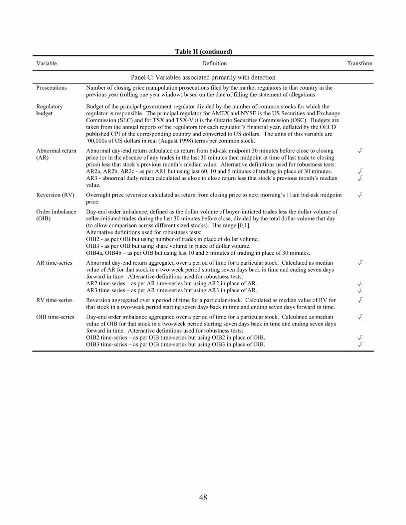
48

Table II (continued)

Variable Definition Transform

Panel C: Variables associated primarily with detection

Prosecutions Number of closing price manipulation prosecutions filed by the market regulators in that country in the previous year (rolling one year window) based on the date of filling the statement of allegations.

Regulatory budget

Budget of the principal government regulator divided by the number of common stocks for which the regulator is responsible. The principal regulator for AMEX and NYSE is the US Securities and Exchange Commission (SEC) and for TSX and TSX-V it is the Ontario Securities Commission (OSC). Budgets are taken from the annual reports of the regulators for each regulator’s financial year, deflated by the OECD published CPI of the corresponding country and converted to US dollars. The units of this variable are ’00,000s of US dollars in real (August 1998) terms per common stock.

Abnormal return (AR)

Abnormal day-end return calculated as return from bid-ask midpoint 30 minutes before close to closing price (or in the absence of any trades in the last 30 minutes then midpoint at time of last trade to closing price) less that stock’s previous month’s median value. Alternative definitions used for robustness tests: AR2a, AR2b, AR2c - as per AR1 but using last 60, 10 and 5 minutes of trading in place of 30 minutes. AR3 - abnormal daily return calculated as close to close return less that stock’s previous month’s median value.

Reversion (RV) Overnight price reversion calculated as return from closing price to next morning’s 11am bid-ask midpoint price.

Order imbalance (OIB)

Day-end order imbalance, defined as the dollar volume of buyer-initiated trades less the dollar volume of seller-initiated trades during the last 30 minutes before close, divided by the total dollar volume that day (to allow comparison across different sized stocks). Has range [0,1]. Alternative definitions used for robustness tests: OIB2 - as per OIB but using number of trades in place of dollar volume. OIB3 - as per OIB but using share volume in place of dollar volume. OIB4a, OIB4b – as per OIB but using last 10 and 5 minutes of trading in place of 30 minutes.

AR time-series Abnormal day-end return aggregated over a period of time for a particular stock. Calculated as median value of AR for that stock in a two-week period starting seven days back in time and ending seven days forward in time. Alternative definitions used for robustness tests: AR2 time-series – as per AR time-series but using AR2 in place of AR. AR3 time-series – as per AR time-series but using AR3 in place of AR.

RV time-series

Reversion aggregated over a period of time for a particular stock. Calculated as median value of RV for that stock in a two-week period starting seven days back in time and ending seven days forward in time.

OIB time-series

Day-end order imbalance aggregated over a period of time for a particular stock. Calculated as median value of OIB for that stock in a two-week period starting seven days back in time and ending seven days forward in time. Alternative definitions used for robustness tests: OIB2 time-series – as per OIB time-series but using OIB2 in place of OIB. OIB3 time-series – as per OIB time-series but using OIB3 in place of OIB.

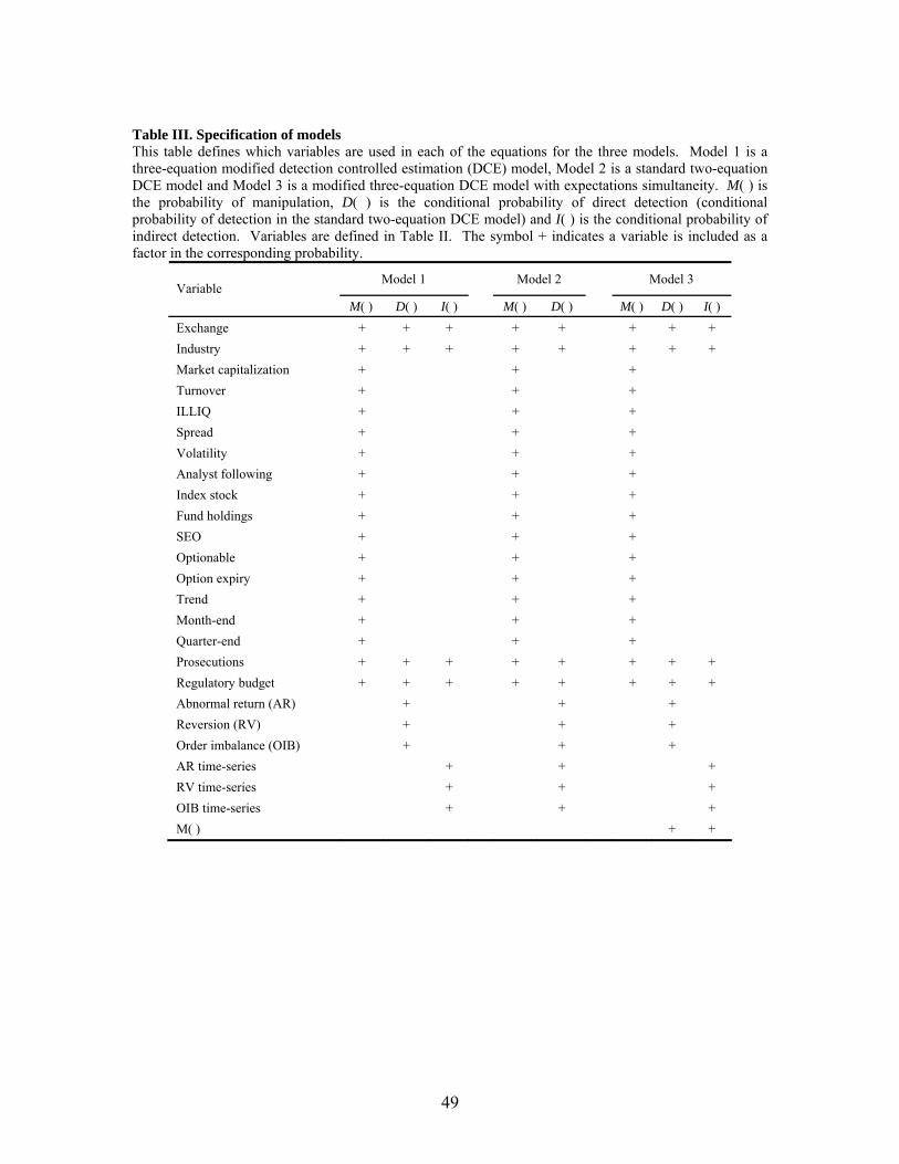
49

Table III. Specification of models This table defines which variables are used in each of the equations for the three models. Model 1 is a three-equation modified detection controlled estimation (DCE) model, Model 2 is a standard two-equation DCE model and Model 3 is a modified three-equation DCE model with expectations simultaneity. M( ) is the probability of manipulation, D( ) is the conditional probability of direct detection (conditional probability of detection in the standard two-equation DCE model) and I( ) is the conditional probability of indirect detection. Variables are defined in Table II. The symbol + indicates a variable is included as a factor in the corresponding probability.

Model 1 Model 2 Model 3 Variable

M( ) D( ) I( ) M( ) D( ) M( ) D( ) I( )

Exchange + + + + + + + +

Industry + + + + + + + +

Market capitalization + + +

Turnover + + +

ILLIQ + + +

Spread + + +

Volatility + + +

Analyst following + + +

Index stock + + +

Fund holdings + + +

SEO + + +

Optionable + + +

Option expiry + + +

Trend + + +

Month-end + + +

Quarter-end + + +

Prosecutions + + + + + + + +

Regulatory budget + + + + + + + +

Abnormal return (AR) + + +

Reversion (RV) + + +

Order imbalance (OIB) + + +

AR time-series + + +

RV time-series + + +

OIB time-series + + +

M( ) + +

50

Table IV. Summary statistics This table reports summary statistics for variables used in the model of manipulation and detection. The variables are defined in Table II. Raw data are actual observed values whereas Normalized and scaled are values after applying normalizing transformations to the variables. Detected manipulation refers to the sample of stock-days in which manipulation has been detected and prosecuted by a regulator (Yes) and the sample of stock-days without detected and prosecuted manipulation (No). Medians and standard deviations (Std dev) are not reported for binary variables. The units of the raw data are in parentheses under the variable names.

Raw data Normalized and scaled

Variable

Detected manipulation Mean Std dev Median Mean Std dev Median

Panel A: Variables associated with both manipulation and detection

Exchange (AMEX) Yes 0.17 0.17 (Binary) No 0.13 0.13

Exchange (TSX) Yes 0.46 0.46 (Binary) No 0.25 0.25

Exchange (TSX-V) Yes 0.20 0.20 (Binary) No 0.05 0.05

Exchange (NYSE) Yes 0.18 0.18 (Binary) No 0.56 0.56

Panel B: Variables associated primarily with manipulation

Market capitalization Yes 442 1,579 67 2.01 0.58 1.83 (USD million) No 2,963 12,737 236 2.39 1.01 2.37

Turnover Yes 0.97 4.98 0.08 4.96 0.61 4.89 (USD million) No 8.07 31.29 0.21 5.43 1.29 5.31

ILLIQ Yes 0.48 0.36 0.47 2.09 1.56 2.02 (% / USD10,000) No 0.36 0.43 0.07 1.54 1.87 0.31

Spread Yes 2.71 1.44 2.56 1.57 0.49 1.60 (%) No 2.32 3.68 0.88 1.22 0.91 0.94

Analyst coverage Yes 1.63 4.42 0.00 0.62 1.12 0.00 (Count) No 3.93 5.94 1.00 1.32 1.48 1.00

Fund holdings Yes 5.45 8.50 1.12 5.45 8.50 1.12 (%) No 11.98 13.2 6.98 11.98 13.2 6.98

Trend Yes 2.81 22.1 1.59 0.21 2.35 1.17 (%) No -0.14 17.5 0.00 0.01 2.06 0.00

Volatility Yes 1.87 1.90 1.48 1.10 0.82 1.21 (%) No 3.39 3.80 2.18 1.67 0.78 1.48

Index stock Yes 0.11 0.11 (Binary) No 0.18 0.18

SEO Yes 0.013 0.013 (Binary) No 0.006 0.006

Optionable Yes 0.09 0.09 (Binary) No 0.28 0.28

Option expiry Yes 0.00 0.00 (Binary) No 0.01 0.01

Month-end Yes 0.31 0.31 (Binary) No 0.05 0.05

Quarter-end Yes 0.20 0.20 (Binary) No 0.02 0.02

51

Table IV (continued)

Raw data Normalized and scaled

Variable

Detected manipulation Mean Std dev Median Mean Std dev Median

Panel C: Variables associated primarily with detection

Prosecutions Yes 0.47 0.66 0.00 0.47 0.66 0.00 (Count) No 0.73 0.99 0.00 0.73 0.99 0.00

Regulatory budget Yes 58.1 75.5 9.80 0.58 0.76 0.10 (USD100,000 / stock) No 130 90.9 165 1.30 0.91 1.65

Abnormal return (AR) Yes 1.24 2.39 0.86 0.72 1.17 0.93 (%) No 0.04 2.54 0.00 0.01 1.06 0.00

Reversion (RV) Yes 1.55 3.72 1.71 0.93 1.40 1.31 (%) No -0.19 3.66 0.00 -0.05 1.39 0.00

Order imbalance (OIB) Yes 0.11 0.25 0.02 0.11 0.25 0.02 (Dimensionless ratio) No 0.00 0.09 0.00 0.00 0.09 0.00

AR time series Yes 0.20 0.77 0.14 0.20 0.72 0.37 (%) No 0.01 1.17 0.00 0.00 0.67 0.00

RV time series Yes 1.15 1.28 1.12 0.81 0.85 1.06 (%) No -0.17 1.78 0.00 -0.06 0.91 0.00

OIB time series Yes 0.01 0.04 0.00 0.15 0.45 0.00 (Dimensionless ratio) No 0.00 0.01 0.00 0.04 0.15 0.00

Observations Yes 184 No 1,249,748

52

Table V. Model estimation This table reports the results of the estimation of the models. Model 1 is a three-equation modified DCE model, Model 2 is a standard two-equation DCE model and Model 3 is a modified three-equation DCE model with expectations simultaneity. M( ) is the probability of manipulation, D( ) is the conditional probability of direct detection (detection in the standard two-equation DCE model) and I( ) is the conditional probability of indirect detection. Variables are defined in Table II. Numbers not in brackets are the coefficient estimates. Numbers in brackets are the marginal effects (partial derivatives of the corresponding probability with respect to each of the variables, reported as a percentage of the estimated corresponding probability). Pseudo R-squared is McFadden’s likelihood ratio index (one minus the ratio of the log-likelihood with all predictors and the log-likelihood with intercepts only). Significance at the 10%, 5% and 1% levels is indicated by *, ** and *** respectively.

Model 1 Model 2 Model 3

Variable M( ) D( ) I( ) M( ) D( ) M( ) D( ) I( )

Regulatory budget -2.01*** 1.69*** 6.48** -2.11*** 1.59*** -2.01*** 1.68** 6.49** (-1.98) (1.63) (6.14) (-2.09) (1.52) (-1.99) (1.62) (6.14)

Analyst coverage -0.37*** -0.42*** -0.38*** (-0.36) (-0.42) (-0.38)

Index stock -1.22*** -1.29*** -1.22*** (-1.21) (-1.28) (-1.21)

Fund holdings -0.08*** -0.09*** -0.08*** (-0.08) (-0.09) (-0.08)

Market capitalization 0.73*** 0.71*** 0.73*** (0.72) (0.71) (0.72)

ILLIQ -0.43*** -0.37*** -0.44*** (-0.43) (-0.37) (-0.44)

Month-end (ME) 1.02*** 0.71** 1.01*** (1.01) (0.70) (0.99)

Quarter-end (QE) 1.09*** 0.70 1.07*** (1.07) (0.69) (1.06)

ME * Fund holdings 0.06*** 0.08*** 0.06*** (0.06) (0.08) (0.06)

QE * Fund holdings 0.04* 0.05* 0.04* (0.04) (0.05) (0.04)

Volatility -0.98*** -0.69*** -0.93*** (-0.97) (-0.69) (-0.92)

Abnormal return (AR) 0.85*** 0.71*** 0.84*** (0.82) (0.68) (0.81)

Reversion (RV) 0.30*** 0.27*** 0.29*** (0.29) (0.25) (0.28)

Order imbalance (OIB) 1.43** 1.10 1.41** (1.37) (1.05) (1.36)

AR time series 3.17*** 0.25 3.18*** (3.00) (0.24) (3.01)

RV time series 7.64*** 1.10*** 7.66*** (7.23) (1.05) (7.24)

OIB time series 3.12 0.03 3.12 (2.95) (0.03) (2.95)

M( ) 0.14*** 0.01Exchange dummies Yes Yes Yes Yes Yes Yes Yes Yes

Observations 1,249,932 1,249,932 1,249,932

Pseudo R-squared 0.23 0.17 0.23

53

Table VI. Bootstrap-based corrections for double-clustered errors and finite-sample bias This table reports the results of Model 1 (the three-equation modified DCE model from Table V) estimated using a reduced random sample and bootstraps of 500 replications each. Double-clustered errors uses a bootstrap algorithm that provides consistent standard error estimates when errors cluster by stock and by date. Bias-corrected estimates uses a bootstrap algorithm that corrects parameter estimates for nonlinear estimator finite-sample bias. M( ) is the probability of manipulation, D( ) is the conditional probability of direct detection and I( ) is the conditional probability of indirect detection. Variables are defined in Table II. Numbers not in brackets are the coefficient estimates. Numbers in brackets are the marginal effects (partial derivatives of the corresponding probability with respect to each of the variables, reported as a percentage of the estimated corresponding probability). Significance at the 10%, 5% and 1% levels is indicated by *, ** and *** respectively.

Double-clustered errors Bias-corrected estimates

Variable M( ) D( ) I( ) M( ) D( ) I( )

Regulatory budget -2.06*** 1.77*** 6.51*** -1.87*** 1.69*** 6.68*** (-2.04) (1.69) (6.18) (-1.86) (1.60) (5.95)

Analyst following -0.12* -0.16* (-0.12) (-0.16)

Index stock -1.22*** -1.24*** (-1.21) (-1.23)

Fund holdings -0.07*** -0.07*** (-0.07) (-0.07)

Market capitalization 0.83*** 0.77*** (0.82) (0.76)

ILLIQ -0.12 -0.14 (-0.12) (-0.14)

Month-end (ME) 1.56*** 1.41*** (1.54) (1.40)

Quarter-end (QE) 1.70*** 1.44*** (1.69) (1.43)

ME * Fund holdings 0.03*** 0.04*** (0.03) (0.04)

QE * Fund holdings 0.01 0.01 (0.01) (0.01)

Volatility -2.37*** -2.05*** (-2.35) (-2.04)

Abnormal return (AR) 1.22*** 1.21*** (1.17) (1.15)

Reversion (RV) 0.45*** 0.45*** (0.43) (0.42)

Order imbalance (OIB) 1.86*** 2.38*** (1.78) (1.24)

AR time series 3.01** 2.14*** (2.86) (3.67)

RV time series 7.79*** 7.47*** (7.40) (7.62)

OIB time series 3.26*** 3.27*** (3.10) (3.06)

Exchange dummies Yes Yes Yes Yes Yes Yes

Observations 12,681 12,681

54

Figure 1. Modified detection controlled estimation model.

Manipulated

Stock-day i

Directly detected

Not manipulated

Indirectly detected

Not directly detected

Not indirectly detected

No detected manipulation (undetected

manipulation and non-

manipulation)

Ac

Detected manipulation

A

11

i

Y

01

i

Y

02

i

Y

12

i

Y

03

i

Y

13

i

Y