Stock Market Analytics Report James Ferris and Zilong Li

December 5th, 2018

An overview of your topic area The growth of data mining and data analysis has huge impact on to the financial

applications and services. Market share information, online transactions and economic factors are easy to find nowadays on the internet. Evaluating the stock market data from the past market trading history is a flexible and reliable way to understand and predict the market movement in the future. To achieve the most accurate market data measurement for the real investment, stock exchange trend analysis requires a large amount of computation and classification to summarize the calculated financial indicators and formed a report including market growing graph, investment suggestion and so on. Parallel paradigm can execute mining observation on large datasets partition for data collection and computation efficiency. This report helps the reader to explore the detail about the data calculation using the parallel programming method and understand the stock movement prediction technique.

A description of the computational problem you solved

The main computational problem for this project is to calculate the financial indicators based on the historical NYSE data from online API. From each share, the proposed model retrieves the daily stock time series between year 1998 and 2018. The expected indicator computation includes EMA (exponential moving average), SMA (simple moving average), RSI (relative strength index) and SO (stochastic oscillator). Once the indicators are generated, we process them and convert them into a general market trend report such as suggested share buy-in/sell-out advice and Chart patterns in both long term and short term future market. An analysis of your first research paper (the same material as in your presentation) [1]

Our first research paper was titled Predictive Analytics on Public Data, and was authored by:

1. Krauss, Jonas, University of Cologne, Pohligstr. 1, 50969 Köln, Germany 2. Schoder, Detlef, University of Cologne, Pohligstr. 1, 50969 Köln, Germany 3. Nann, Stefan, University of Cologne, Pohligstr. 1, 50969 Köln, Germany

This paper explored the possibility of determining price action based on the sentiment received from several public API’s including Twitter and Yahoo Finance. After parsing the data to

determine whether the sentiment was positive or negative, and to which stock it is referring, the group calculated their predictor using the following formula:

Based on the above formula, a positive sentiment would trigger a buy action, and a negative sentiment would trigger a sell action. Over a four month period, the group implemented their model and found that they received a 400% ROI (return on investment). This is a huge ROI that isn’t typical of a lot of strategies and works toward proving that public sentiment can and should be considered when working with stock analytics. An analysis of your second research paper [2]

Our second research paper was The Effect of Rating Changes on Stock Returns, authored by Dr. Imran Ahmad Khan, Assistant Professor, College of Administrative and Financial Sciences, Saudi Electronic University, Dammam, Saudi Arabia. This paper covered the effect that rating changes on a company would have on the price of the stock, specifically in India. A rating change would be announced by a reputable company or individual that puts out public ratings (buy,sell,hold) on a stock. Dr. Khan found that between 2004-2017, rating changes on stocks in India had a significant effect on the volatility of the price for a short time after the rating change. An analysis of your third research paper [3]

In the Equity Forecast paper (ref#1), written by Nikola Milosevic from school of Computer Science in University of Manchester, he has raised the question stock price movement and suggested using the machine learning methods to process many financial indicator and evaluate them. The paper describes the equity price movement prediction by classifying stock into two categories: good and bad. The Machine learning trainer in this paper utilize the Naïve Bayes algorithm to determine stocks that will rise over 10% in a period of one year. Of course, the rise ratio and the estimate time frame are the variable factors which can be interchange depends on the user’s preferences. This paper specifies the data classification with the computed financial indicator values between two consecutive years of a stock. If the stock in the current year is 10% higher than the previous year, the machine learning model categorize the financial indicator to the good class. Otherwise, those growth indicators are put to bad class. Then, the calculation process generates the probability of both good and bad data using Naïve Bayes Classifier. By Compare the good and bad probability, the trainer determines the stock price

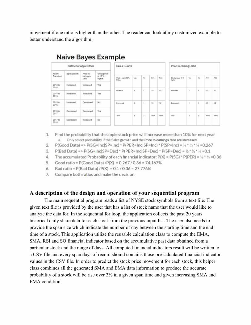
movement if one ratio is higher than the other. The reader can look at my customized example to better understand the algorithm.

A description of the design and operation of your sequential program

The main sequential program reads a list of NYSE stock symbols from a text file. The given text file is provided by the user that has a list of stock name that the user would like to analyze the data for. In the sequential for loop, the application collects the past 20 years historical daily share data for each stock from the previous input list. The user also needs to provide the span size which indicate the number of day between the starting time and the end time of a stock. This application utilize the reusable calculation class to compute the EMA, SMA, RSI and SO financial indicator based on the accumulative past data obtained from a particular stock and the range of days. All computed financial indicators result will be written to a CSV file and every span days of record should contains those pre-calculated financial indicator values in the CSV file. In order to predict the stock price movement for each stock, this helper class combines all the generated SMA and EMA data information to produce the accurate probability of a stock will be rise over 2% in a given span time and given increasing SMA and EMA condition.

A description of the design and operation of your parallel program

The main parallel program reads a list of NYSE stock symbols from a text file. The given text file is provided by the user that has a list of stock name that the user would like to analyze the data for. In the parallel for loop, the application collects the past 20 years historical daily share data for each stock from the previous input list. The user also needs to provide the span size which indicate the number of day between the starting time and the end time of a stock. This application utilize the reusable calculation class to compute the EMA, SMA, RSI and SO financial indicator based on the accumulative past data obtained from a particular stock and the range of days. All computed financial indicators result will be written to a CSV file and every span days of record should contains those pre-calculated financial indicator values in the CSV file. In order to predict the stock price movement for each stock, this helper class combines all the generated SMA and EMA data information to produce the accurate probability of a stock will be rise over 2% in a given span time and given increasing SMA and EMA condition.

This design is exactly the same as the sequential version, however now the stocks are dealt with in parallel.

A developer's manual (i.e. exact instructions for how to compile the software)

1. Download PJ2.jar file and the Java JDK development package. 2. Use the following command to set the classpath for the parallel Java jar file.

a. export CLASSPATH=.:/var/tmp/parajava/pj2/pj2.jar 3. Add the JDK bin directory to the build path.

a. export PATH=/usr/local/dcs/versions/jdk1.7.0_51/bin:$PATH 4. Download the source project from GitHub link:

https://github.com/jef1771/StockMarketAnalysis 5. In the terminal application, the user changes directory to

/StockMarketAnalysis/Stocks_Java/Src folder. 6. Run the Java compilation command to generate the JAR file

a. javac *.java b. jar cf p4.jar *.class

7. To execute this both sequential and parallel applications, the user execute the following command format.

a. java pj2 debug=makespan jar=<jar> MainSequential <symbol file path> <time span>

b. java pj2 threads=<nt> debug=makespan jar=<jar> MainParallel <symbol file path> <time span>

A user's manual (i.e. exact instructions for how to run the software, how to use the UI, screen shots, etc.)

1. Download PJ2.jar file and the Java JDK development package. 2. Use the following command to set the classpath for the parallel Java jar file.

a. export CLASSPATH=.:/var/tmp/parajava/pj2/pj2.jar 3. Add the JDK bin directory to the build path.

a. export PATH=/usr/local/dcs/versions/jdk1.7.0_51/bin:$PATH 4. Download the source project from GitHub link:

https://github.com/jef1771/StockMarketAnalysis 5. In the terminal application, the user changes directory to

/StockMarketAnalysis/Stocks_Java/Src folder. 6. Run the Java compilation command to generate the JAR file

a. javac *.java b. jar cf p4.jar *.class

7. To execute this both sequential and parallel applications, the user execute the following command format.

a. java pj2 debug=makespan jar=<jar> MainSequential <symbol file path> <time span>

b. java pj2 threads=<nt> debug=makespan jar=<jar> MainParallel <symbol file path> <time span>

Generated sample output files and their format:

The strong scaling performance data (the same tables and plots as in your presentation) N (# Stocks) K (cores) T (ms) Speedup Efficiency

50 sequential 3648

1 4074 0.8954344624 0.8954344624

2 2478 1.472154964 0.7360774818

3 1899 1.921011058 0.6403370195

4 1720 2.120930233 0.5302325581

5 1614 2.260223048 0.4520446097

6 1476 2.471544715  0.4119241192

7 1384 2.63583815 0.3765483072

8 1321 2.761544285 0.3451930356

9 1272 2.867924528 0.3186582809

10 1222 2.985270049 0.2985270049

11 1252 2.913738019 0.2648852745

12 1269 2.874704492 0.2395587076

N (# Stocks) K (cores) T (ms) Speedup Efficiency

250 sequential 14786

1 14615 1.011700308 1.011700308

2 7462 1.981506299 0.9907531493

3 5601 2.639885735 0.8799619116

4 4568 3.236865149 0.8092162872

5 3972 3.722557905 0.7445115811

6 3588 4.120958751 0.6868264586

7 3513 4.208938229 0.6012768899

8 3078 4.803768681 0.6004710851

9 2880 5.134027778 0.5704475309

10 2851 5.186250438 0.5186250438

11 2535 5.832741617 0.5302492379

12 2518 5.872120731 0.4893433942

N (# Stocks) K (cores) T (ms) Speedup Efficiency

500 sequential 28189

1 27848 1.012245045 1.012245045

2 14639 1.925609673 0.9628048364

3 10549 2.672196417 0.8907321389

4 7972 3.536001004 0.8840002509

5 6976 4.040854358 0.8081708716

6 6006 4.693473193 0.7822455322

7 5701 4.944571128 0.706367304

8 5028 5.606404137 0.7008005171

9 4864 5.795435855 0.6439373173

10 4466 6.311912226 0.6311912226

11 4351 6.478740519 0.5889764109

12 4016 7.019173307 0.5849311089

N (# Stocks) K (cores) T (ms) Speedup Efficiency

1000 sequential 54897

1 53047 1.034874734 1.034874734

2 27869 1.969823101 0.9849115505

3 19817 2.770197305 0.9233991018

4 15509 3.539686634 0.8849216584

5 13240 4.146299094 0.8292598187

6 11321 4.849129936 0.8081883226

7 10842 5.063364693 0.7233378133

8 8951 6.133057759 0.7666322199

9 8640 6.353819444 0.7059799383

10 8095 6.781593576 0.6781593576

11 7520 7.300132979 0.6636484526

12 6977 7.868281496 0.6556901247

N (# Stocks) K (cores) T (ms) Speedup Efficiency

5000 sequential 280289

1 265896 1.054130186 1.054130186

2 132832 2.110101482 1.055050741

3 91105 3.076549037 1.025516346

4 69416 4.037815489 1.009453872

5 58461 4.794461265 0.958892253

6 49569 5.654521979 0.9424203299

7 44858 6.248361496 0.8926230709

8 40535 6.914740348 0.8643425435

9 36557 7.667177285 0.8519085872

10 34035 8.235316586 0.8235316586

11 31589 8.872993764 0.8066357967

12 29888 9.377977784 0.7814981486

An explanation of why any nonideal strong scaling is occurring

Unfortunately, the only part of our program that we found could be parallelized was processing each stock symbol. This has a large sequential dependency of reading in a very large text file with the stock data, loading that data into java objects, running calculations on the data, and then outputting to another file. All of the calculations such as the RSI, SO, EMA, and SMA also have sequential dependencies, and can’t be done in parallel.

As expected, as the dataset got larger, the strong scaling become closer to the ideal. This is because with more computation time among more stocks, the sequential part of the program becomes dwarfed by the parallel part. The weak scaling performance data (the same tables and plots as in your presentation) N(1) N K T(msec) Sizeup Efficiency

50 50 seq 3511

50 1 3747 0.9370162797 0.9370162797

100 2 4039 1.738549146 0.8692745729

200 4 4011 3.501371229 0.8753428073

500 10 4540 7.733480176 0.7733480176

600 12 5080 8.293700787 0.6911417323

N(1) N K T(msec) Sizeup Efficiency

100 100 seq 6838

100 1 7018 0.9743516671 0.9743516671

200 2 6093 2.244542918 1.122271459

400 4 6888 3.970963995 0.9927409988

1000 10 7710 8.869001297 0.8869001297

1200 12 8898 9.221847606 0.7684873005

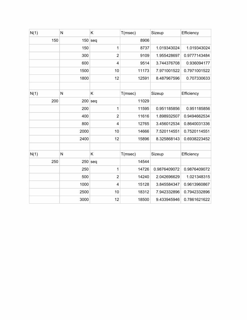
N(1) N K T(msec) Sizeup Efficiency

150 150 seq 8906

150 1 8737 1.019343024 1.019343024

300 2 9109 1.955428697 0.9777143484

600 4 9514 3.744376708 0.936094177

1500 10 11173 7.971001522 0.7971001522

1800 12 12591 8.487967596 0.707330633

N(1) N K T(msec) Sizeup Efficiency

200 200 seq 11029

200 1 11595 0.951185856 0.951185856

400 2 11616 1.898932507 0.9494662534

800 4 12765 3.456012534 0.8640031336

2000 10 14666 7.520114551 0.7520114551

2400 12 15896 8.325868143 0.6938223452

N(1) N K T(msec) Sizeup Efficiency

250 250 seq 14544

250 1 14726 0.9876409072 0.9876409072

500 2 14240 2.042696629 1.021348315

1000 4 15128 3.845584347 0.9613960867

2500 10 18312 7.942332896 0.7942332896

3000 12 18500 9.433945946 0.7861621622

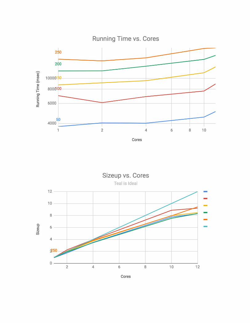
An explanation of why any nonideal weak scaling is occurring

We had a similar problem with the weak scaling as we did with the strong scaling. Our large sequential dependencies prevent us from seeing ideal sizeups and efficiencies. Also as with strong scaling, we are seeing diminishing returns as we add more cores. This seems to be because of the large sequential dependency, the additional overhead with more cores just prolongs the sequential part of the program. A discussion of possible future work

Additional work that we would like to see done with our model would be verification/testing, additional technology, and additional model parameters.

By verification and testing, we mean that we would like to see our model making predictions in real time, and investigate its accuracy over a span of a few months. As the team did in our first research paper, we would like to see what our Return on Investment would be using our model.

Additional technology could include additional accelerators such as a GPU. Using a GPU to carry out the technical indicator calculations would most likely prove to add additional speedup and efficiency to our program.

Finally, for additional model parameters, we would like to add in additional indicators as the teams from our first and second research papers did. We would like to be able to include

some sentiment indicators from the general public, as well as some predictions based on reputable companies providing rating changes. A discussion of what you learned from the project

1. We have learned financial/Stock price measurement related knowledge such as calculating the financial indicator based on the historical daily stock information.

2. Based on the runtime performance of the parallel application, we realize that the read/write file process will impact the strong scaling and weak scaling runtime. There is a lot of overhead when reading the stock price data and stock symbols from a text/csv file.

A statement of what each individual team member did on the project

James wrote the python scripts to pull the stock data from the internet. The scripts included requests to pull the raw data, and then parsing through that data in order to convert into our desired format. James also wrote the Calculations part of the Java program. This program included a way to calculate the Exponential Moving Average (EMA), Simple Moving Average (SMA), Relative Strength Index (RSI), and the Stochastic Oscillator. With all of these calculations, Li was able to implement his part.

Li wrote the basic utility class(helper.java) to do the read stock data from the database and write the report analysis to the CSV file to record the financial indicator for each stock. Li was also able to reuse the result calculated from James program with Naive Bayes Machine learning trainer to generate a suggested stock price and its probability on rising in a given period of time.

References [1] Nann, Stefan; Krauss, Jonas; Schoder, Detlef “Predictive analytics on public data-The case of stock markets.” June 2013, https://www.researchgate.net/publication/260190081_Predictive_analytics_on_public_data-The_case_of_stock_markets [2] Dr. Imran Ahmad Khan “The Effect of Rating Changes on Stock Returns: An Empirical Investigation”, March 2018, http://www.academia.edu/37452762/The_Effect_of_Rating_Changes_on_Stock_Returns_An_Empirical_Investigation [3] Milosevic, Nikola. “Equity Forecast: Predicting Long Term Stock Price Movement Using Machine Learning.” Equity Forecast: Predicting Long Term Stock Price Movement Using Machine Learning, Arxiv.org, 2 Mar. 2016, https://arxiv.org/abs/1603.00751