Stochastic Simulation of Processes, Fields and Structures...One of the simplest stochastic processes...
157
Stochastic Simulation of Processes, Fields and Structures Ulm University Institute of Stochastics Lecture Notes Dr. Tim Brereton Summer Term 2014 Ulm, 2014
Transcript of Stochastic Simulation of Processes, Fields and Structures...One of the simplest stochastic processes...

Stochastic Simulation ofProcesses, Fields and
Structures
Ulm University
Institute of Stochastics
Lecture Notes
Dr. Tim Brereton
Summer Term 2014
Ulm, 2014

2
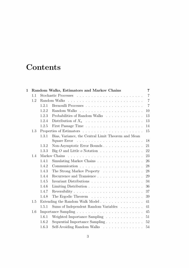
Contents
1 Random Walks, Estimators and Markov Chains 7
1.1 Stochastic Processes . . . . . . . . . . . . . . . . . . . . . . . 7
1.2 Random Walks . . . . . . . . . . . . . . . . . . . . . . . . . . 7
1.2.1 Bernoulli Processes . . . . . . . . . . . . . . . . . . . . 7
1.2.2 Random Walks . . . . . . . . . . . . . . . . . . . . . . 10
1.2.3 Probabilities of Random Walks . . . . . . . . . . . . . 13
1.2.4 Distribution of Xn . . . . . . . . . . . . . . . . . . . . 13
1.2.5 First Passage Time . . . . . . . . . . . . . . . . . . . . 14
1.3 Properties of Estimators . . . . . . . . . . . . . . . . . . . . . 15
1.3.1 Bias, Variance, the Central Limit Theorem and MeanSquare Error . . . . . . . . . . . . . . . . . . . . . . . 18
1.3.2 Non-Asymptotic Error Bounds . . . . . . . . . . . . . . 21
1.3.3 Big O and Little o Notation . . . . . . . . . . . . . . . 22
1.4 Markov Chains . . . . . . . . . . . . . . . . . . . . . . . . . . 23
1.4.1 Simulating Markov Chains . . . . . . . . . . . . . . . . 26
1.4.2 Communication . . . . . . . . . . . . . . . . . . . . . . 28
1.4.3 The Strong Markov Property . . . . . . . . . . . . . . 28
1.4.4 Recurrence and Transience . . . . . . . . . . . . . . . . 29
1.4.5 Invariant Distributions . . . . . . . . . . . . . . . . . . 34
1.4.6 Limiting Distribution . . . . . . . . . . . . . . . . . . . 36
1.4.7 Reversibility . . . . . . . . . . . . . . . . . . . . . . . . 37
1.4.8 The Ergodic Theorem . . . . . . . . . . . . . . . . . . 39
1.5 Extending the Random Walk Model . . . . . . . . . . . . . . . 41
1.5.1 Sums of Independent Random Variables . . . . . . . . 41
1.6 Importance Sampling . . . . . . . . . . . . . . . . . . . . . . . 45
1.6.1 Weighted Importance Sampling . . . . . . . . . . . . . 51
1.6.2 Sequential Importance Sampling . . . . . . . . . . . . . 52
1.6.3 Self-Avoiding Random Walks . . . . . . . . . . . . . . 54
3

4 CONTENTS
2 Poisson Processes and Continuous Time Markov Chains 632.1 Stochastic Processes in Continuous Time . . . . . . . . . . . . 632.2 The Poisson Process . . . . . . . . . . . . . . . . . . . . . . . 65
2.2.1 Point Processes on [0,∞) . . . . . . . . . . . . . . . . 652.2.2 Poisson Process . . . . . . . . . . . . . . . . . . . . . . 672.2.3 Order Statistics and the Distribution of Arrival Times 702.2.4 Simulating Poisson Processes . . . . . . . . . . . . . . 722.2.5 Inhomogenous Poisson Processes . . . . . . . . . . . . 742.2.6 Simulating an Inhomogenous Poisson Process . . . . . 752.2.7 Compound Poisson Processes . . . . . . . . . . . . . . 77
2.3 Continuous Time Markov Chains . . . . . . . . . . . . . . . . 782.3.1 Transition Function . . . . . . . . . . . . . . . . . . . . 792.3.2 Infinitesimal Generator . . . . . . . . . . . . . . . . . . 802.3.3 Continuous Time Markov Chains . . . . . . . . . . . . 802.3.4 The Jump Chain and Holding Times . . . . . . . . . . 802.3.5 Examples of Continuous Time Markov Chains . . . . . 812.3.6 Simulating Continuous Time Markov Chains . . . . . . 822.3.7 The Relationship Between P and Q in the Finite Case 842.3.8 Irreducibility, Recurrence and Positive Recurrence . . . 852.3.9 Invariant Measures and Stationary Distribution . . . . 862.3.10 Reversibility and Detailed Balance . . . . . . . . . . . 87
3 Gaussian Processes and Stochastic Differential Equations 893.1 Gaussian Processes . . . . . . . . . . . . . . . . . . . . . . . . 89
3.1.1 The Multivariate Normal Distribution . . . . . . . . . 893.1.2 Simulating a Gaussian Processes Version 1 . . . . . . . 943.1.3 Stationary and Weak Stationary Gaussian Processes . . 983.1.4 Finite Dimensional Distributions . . . . . . . . . . . . 1033.1.5 Marginal and Conditional Multivariate Normal Distri-
butions . . . . . . . . . . . . . . . . . . . . . . . . . . . 1043.1.6 Interpolating Gaussian Processes . . . . . . . . . . . . 1053.1.7 Markovian Gaussian Processes . . . . . . . . . . . . . . 106
3.2 Brownian Motion . . . . . . . . . . . . . . . . . . . . . . . . . 1083.2.1 Existence . . . . . . . . . . . . . . . . . . . . . . . . . 1113.2.2 Some useful results . . . . . . . . . . . . . . . . . . . . 1153.2.3 Integration With Respect to Brownian Motion . . . . . 116
3.3 Stochastic Differential Equations . . . . . . . . . . . . . . . . 1163.3.1 Ito’s Lemma . . . . . . . . . . . . . . . . . . . . . . . . 1173.3.2 Numerical Solutions of SDEs . . . . . . . . . . . . . . . 1173.3.3 Multidimensional SDEs . . . . . . . . . . . . . . . . . . 121
3.4 Existence and Uniqueness Result . . . . . . . . . . . . . . . . 123
CONTENTS 5
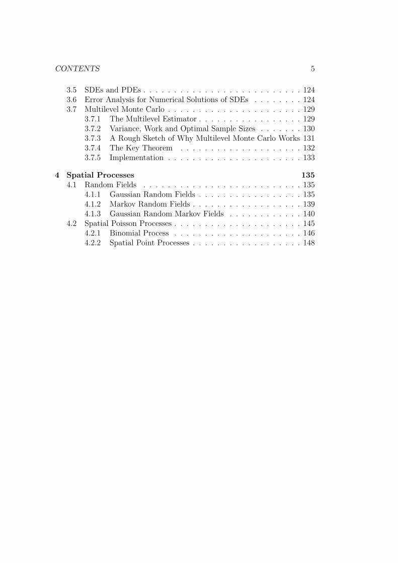
3.5 SDEs and PDEs . . . . . . . . . . . . . . . . . . . . . . . . . . 1243.6 Error Analysis for Numerical Solutions of SDEs . . . . . . . . 1243.7 Multilevel Monte Carlo . . . . . . . . . . . . . . . . . . . . . . 129
3.7.1 The Multilevel Estimator . . . . . . . . . . . . . . . . . 1293.7.2 Variance, Work and Optimal Sample Sizes . . . . . . . 1303.7.3 A Rough Sketch of Why Multilevel Monte Carlo Works 1313.7.4 The Key Theorem . . . . . . . . . . . . . . . . . . . . 1323.7.5 Implementation . . . . . . . . . . . . . . . . . . . . . . 133
4 Spatial Processes 1354.1 Random Fields . . . . . . . . . . . . . . . . . . . . . . . . . . 135
4.1.1 Gaussian Random Fields . . . . . . . . . . . . . . . . . 1354.1.2 Markov Random Fields . . . . . . . . . . . . . . . . . . 1394.1.3 Gaussian Random Markov Fields . . . . . . . . . . . . 140
4.2 Spatial Poisson Processes . . . . . . . . . . . . . . . . . . . . . 1454.2.1 Binomial Process . . . . . . . . . . . . . . . . . . . . . 1464.2.2 Spatial Point Processes . . . . . . . . . . . . . . . . . . 148

6 CONTENTS

Chapter 1
Random Walks, Estimators andMarkov Chains
1.1 Stochastic Processes
To begin, we need to define the basic objects we will be learning about.
Definition 1.1.1 (Stochastic Process). A stochastic process is a set of ran-dom variables Xii∈I , taking values in a state space X , with index sex I ⊂ R.
In general, i represents a point in time. However, it could represent apoint in 1D space as well.
We will say a process is discrete time if I is discrete. For example, Icould be N or 1, 2, 3, 10, 20. Normally, when we talk about discrete timestochastic processes, we will use the index n (e.g., Xnn∈N).
We will say a process is continuous time if I is an interval. For example[0,∞) or [1, 2]. Normally, when we talk about continuous time stochasticprocesses, we will use the index t (e.g. Xtt∈[0,T ]).
1.2 Random Walks
1.2.1 Bernoulli Processes
One of the simplest stochastic processes is a random walk. However, eventhough the random walk is very simple, it has a number of properties that willbe important when we think about more complicated processes. To definea random walk, we begin with an even simpler process called a Bernoulli
process. A Bernoulli process is a discrete time process taking values in thestate space 0, 1.
7

8 CHAPTER 1. RANDOM WALKS ETC.
Definition 1.2.1 (Bernoulli Process). A Bernoulli process with parameterp ∈ [0, 1] is a sequence of independent and identically distributed (i.i.d.) ran-dom variables, Ynn≥1, such that
P(Y1 = 1) = 1− P(Y1 = 0) = p. (1.1)
A variable with the probability mass function (pmf) described by (1.1) iscalled a Bernoulli random variable with distribution Ber(p).
In the case where p = 1/2, you can think of a Bernoulli process as asequence of fair coin tosses. In the case where p 6= 1/2, you can think of aBernoulli process as a sequence of tosses of an unfair coin.
Note that if U ∼ U(0, 1), then P(U ≤ p) = p for p ∈ [0, 1]. This meansif we define the random variable Y = I(U ≤ p), where I(·) is the indicatorfunction and U ∼ U(0, 1), we have
P(Y = 1) = 1− P(Y = 0) = p.
In Matlab, we can make these variables as follows.
Listing 1.1: Generating a Bernoulli Random Variable
1 Y = (rand <= p)
If we want to make a realization of the first n steps of a Bernoulli process,we simply make n such variables. One way to do this is the following.
Listing 1.2: Generating a Bernoulli Process 1
1 n = 20; p = 0.6; Y = zeros(n,1);
2
3 for i = 1:n
4 Y(i) = (rand <= p);
5 end
We can do this more quickly in Matlab though.
Listing 1.3: Generating a Bernoulli Process 2
1 n = 20; p = 0.6;
2
3 Y = (rand(n,1) <= p);
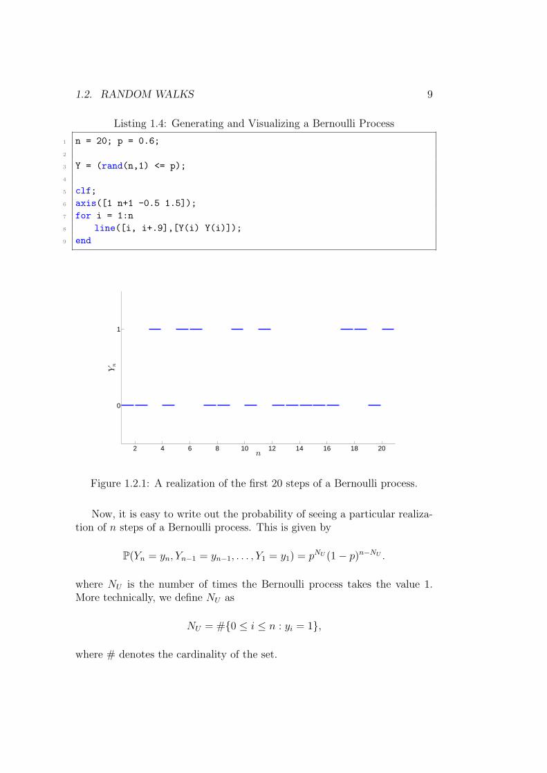
It is important to be able to visualize stochastic objects. One way torepresent / visualize a Bernoulli process is to put n = 1, 2, . . . on the x-axisand the values of Yn on the y-axis. I draw a line (almost of length 1) at eachvalue of Yn, as this is easier to see than dots. Figure 1.2.1 shows a realizationof the first 20 steps of a Bernoulli process.
1.2. RANDOM WALKS 9
Listing 1.4: Generating and Visualizing a Bernoulli Process
1 n = 20; p = 0.6;
2
3 Y = (rand(n,1) <= p);
4
5 clf;
6 axis([1 n+1 -0.5 1.5]);
7 for i = 1:n
8 line([i, i+.9],[Y(i) Y(i)]);
9 end
2 4 6 8 10 12 14 16 18 20
0
1
n
Yn
Figure 1.2.1: A realization of the first 20 steps of a Bernoulli process.
Now, it is easy to write out the probability of seeing a particular realiza-tion of n steps of a Bernoulli process. This is given by
P(Yn = yn, Yn−1 = yn−1, . . . , Y1 = y1) = pNU (1− p)n−NU .
where NU is the number of times the Bernoulli process takes the value 1.More technically, we define NU as
NU = #0 ≤ i ≤ n : yi = 1,
where # denotes the cardinality of the set.

10 CHAPTER 1. RANDOM WALKS ETC.
1.2.2 Random Walks
Now that we can generate Bernoulli processes, we are ready to considerour main object of interest in this chapter: the random walk. The randomwalk is a discrete time random process taking values in the state space Z.
Definition 1.2.2 (Random Walk). Given a Bernoulli process Ynn≥1 withparameter p, we define a random walk Xnn≥0 with parameter p and initialcondition X0 = x0 by
Xn+1 = Xn + (2Yn+1 − 1).
Note that (2Yn − 1) is 1 if Yn = 1 and −1 if Yn = 0. So, essentially, ateach step of the process, it goes up or down by 1.
There are lots of ways to think about random walks. One way is in termsof gambling (which is a classical setting for probability). Think of a gamewhich is free to enter. The person running the game flips a coin. Withprobability p, the coin shows heads and you win AC1. With probability 1− p,you lose AC1. If you start with ACx0, and assuming you can go into debt, Xn
is the random variable describing how much money you have after n games.Given that we know how to generate a Bernoulli process, it is straight-
forward to generate a random walk.
Listing 1.5: Generating a Random Walk 1
1 n = 100; X = zeros(n,1);
2 p = 0.5; X_0 = 0;
3
4 Y = (rand(n,1) <= p);
5 X(1) = X_0 + 2*Y(1) - 1;
6 for i = 2:n
7 X(i) = X(i-1) + 2*Y(i) - 1;
8 end
A more compact way is as follows.
Listing 1.6: Generating a Random Walk 2
1 n = 100; X = zeros(n,1);
2 p = 0.5; X_0 = 0;
3
4 Y = (rand(n,1) <= p);
5 X = X_0 + cumsum((2*Y - 1));
It is good to be able to plot these. Here, we have at least two options.One is to draw a line for each value of Xn, as we did for the Bernoulli process.

1.2. RANDOM WALKS 11
Because the value of Xnn≥0 changes at every value of n, we can draw thelines to be length 1. This approach is nice, because it reinforces the idea thatXnn≥0 jumps at each value of n (this is made obvious by the gaps betweenthe lines).
Listing 1.7: Plotting a Random Walk 1
1 clf
2 axis([1 n+1 min(X)-1 max(X)+1]);
3 for i = 1:n
4 line([i,i+1],[X(i) X(i)],’LineWidth’,3);
5 end
For larger values of n, it is help to draw vertical lines as well as horizontallines (otherwise, things get a bit hard to see). We can do this as follows.
Listing 1.8: Plotting a Random Walk 2
1 clf
2 stairs(X);
3 axis([1 n+1 min(X)-1 max(X)+1]);
Below are a number of realizations of random walks. Figures 1.2.2 and1.2.3 are generated using lines. Figures 1.2.4 and 1.2.5 are generated usingthe ‘stairs’ function.
2 4 6 8 10 12 14 16 18 20−5
−4
−3
−2
−1
0
1
2
n
Xn
Figure 1.2.2: A realization of the first 20 steps of a random walk with p = 0.5.
Note how, as the number of steps simulated gets bigger, the sample pathslook wilder and wilder.

12 CHAPTER 1. RANDOM WALKS ETC.
2 4 6 8 10 12 14 16 18 200
2
4
6
8
10
12
14
16
n
Xn
Figure 1.2.3: A realization of the first 20 steps of a random walk with p = 0.9.
10 20 30 40 50 60 70 80 90 100
−6
−4
−2
0
2
4
6
8
n
Xn
Figure 1.2.4: A realization of the first 100 steps of a random walk withp = 0.5.
1000 2000 3000 4000 5000 6000 7000 8000 9000 10000
−20
0
20
40
60
80
n
Xn
Figure 1.2.5: A realization of the first 10000 steps of a random walk withp = 0.5.

1.2. RANDOM WALKS 13
1.2.3 Probabilities of Random Walks
A random walk is a special kind of process, called a Markov process.Discrete time discrete state space Markov processes (called Markov chains)are defined by the following property.
Definition 1.2.3 (Markov Property: Discrete Time Discrete State SpaceVersion). We say a discrete time, discrete state space stochastic process,Xnn≥0, has the Markov property if
P(Xn+1 = xn+1 |Xn = xn, . . . , X0 = x0) = P(Xn+1 = xn+1 |Xn = xn),
for all n ≥ 0 and x0, . . . , xn ∈ X .
If we think about how a random walk can move after n steps (assumingwe know the values of the first n steps), we have
P(Xn+1 = xn+1 |Xn = xn, . . . , X0 = x0) =
p if xn+1 = xn + 1,
1− p if xn+1 = xn − 1,
0 otherwise.
Note that these probabilities do not depend on any value other than Xn.That is, it is always the case that P(Xn+1 = xn+1 |Xn = xn, . . . , X0 = x0) =P(Xn+1 = xn+1 |Xn = xn), so Xnn≥0 is a Markov chain.
Using this result, we can assign probabilities to various paths of the ran-dom walk. That is, we can write
P(Xn = xn, Xn−1 = xn−1, . . . , X1 = x1)
= P(Xn = xn|Xn−1 = xn−1, . . . , X1 = x1) · · ·P(X2 = x2|X1 = x1)P(X1 = x1)
= P(Xn = xn|Xn−1 = xn−1) · · ·P(X2 = x2|X1 = x1)P(X1 = x1)
Now, each of these probabilities is either p or 1− p. So, we can write
P(Xn = xn, Xn−1 = xn−1, . . . , X1 = x1) = pNU (1− p)n−NU .
where NU is the number of times the random walk goes up. More precisely,
NU = #1 ≤ i ≤ n : xi − xi−1 = 1
1.2.4 Distribution of Xn
One thing we might be interested in is the distribution of Xn, given weonly know the initial value of the random walk, x0. We can make this a bit

14 CHAPTER 1. RANDOM WALKS ETC.
simpler by thinking about the distribution ofXn−x0 (this always starts at 0).Notice that Xn cannot be more than n steps from x0. That is, |Xn−x0| ≤ n.Also, if x0 is even then Xn must be even if n is even and odd if n is odd. Ifx0 is odd, it is the other way around.
Now, Xn − x0 = n can only happen if all n of the steps are up. There isonly one possible path for which this is true. This path has probability pn.Likewise, Xn−x0 = n− 2 can only happen if all but one of the steps are up.Any path for which this is true has probability pn−1(1− p)1. However, thereis more than one path that has n−1 up steps and 1 down step (the first stepcould be the down one or the second step could be the down one, etc.). Infact, there are
(n
n−1
)possible paths. Continuing with this pattern, we have
P(Xn − x0 = x)
=
(n
(n+x)/2
)p(n+x)/2(1− p)(n−x)/2 if |x| ≤ n and x have the same parity as n
0 otherwise.
Having the same parity means both n and x are even or both n and x areodd.
1.2.5 First Passage Time
A quantity we are often very interested in is the first passage time ofXnn≥0 into the set A.
Definition 1.2.4 (First Passage Time: Discrete Time Version). Given astochastic process Xnn≥0 we define the first passage time of Xnn≥0 intothe set A by
τA =
infn ≥ 0 : Xn ∈ A if Xn ∈ A for some n ≥ 0
∞ if Xn /∈ A for all n ≥ 0.
Note that a first passage time is a random variable.In general, for random walks, we want to calculate the first time the
process hits a certain level (say 10). In this case, A = 10, 11, . . .. In arandom walk context, a first passage time could correspond to the first timea queue gets too long, or (in a very simplistic model) the first time a stockprice hits a certain level.
It is possible to work out the distribution of the first passage time usinga beautiful and simple piece of mathematics called the reflection principle.However, I will just give you the result.
1.3. PROPERTIES OF ESTIMATORS 15
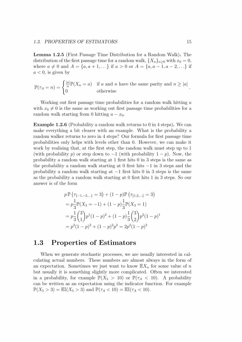
Lemma 1.2.5 (First Passage Time Distribution for a Random Walk). Thedistribution of the first passage time for a random walk, Xnn≥0 with x0 = 0,where a 6= 0 and A = a, a + 1, . . . if a > 0 or A = a, a − 1, a − 2, . . . ifa < 0, is given by
P(τA = n) =
|a|nP(Xn = a) if a and n have the same parity and n ≥ |a|
0 otherwise.
Working out first passage time probabilities for a random walk hitting awith x0 6= 0 is the same as working out first passage time probabilities for arandom walk starting from 0 hitting a− x0.
Example 1.2.6 (Probability a random walk returns to 0 in 4 steps). We canmake everything a bit clearer with an example. What is the probability arandom walker returns to zero in 4 steps? Our formula for first passage timeprobabilities only helps with levels other than 0. However, we can make itwork by realising that, at the first step, the random walk must step up to 1(with probability p) or step down to −1 (with probability 1 − p). Now, theprobability a random walk starting at 1 first hits 0 in 3 steps is the same asthe probability a random walk starting at 0 first hits −1 in 3 steps and theprobability a random walk starting at −1 first hits 0 in 3 steps is the sameas the probability a random walk starting at 0 first hits 1 in 3 steps. So ouranswer is of the form
pP(τ−1,−2,... = 3
)+ (1− p)P
(τ1,2,... = 3
)
= p1
3P(X3 = −1) + (1− p)
1
3P(X3 = 1)
= p1
3
(3
1
)p1(1− p)2 + (1− p)
1
3
(3
2
)p2(1− p)1
= p2(1− p)2 + (1− p)2p2 = 2p2(1− p)2
1.3 Properties of Estimators
When we generate stochastic processes, we are usually interested in cal-culating actual numbers. These numbers are almost always in the form ofan expectation. Sometimes we just want to know EXn for some value of nbut usually it is something slightly more complicated. Often we interestedin a probability, for example P(X5 > 10) or P(τA < 10). A probabilitycan be written as an expectation using the indicator function. For exampleP(X5 > 3) = EI(X5 > 3) and P(τA < 10) = EI(τA < 10).
16 CHAPTER 1. RANDOM WALKS ETC.
In general, we will not know how to calculate the expectations we areinterested in explicitly. In the first few weeks we will practice by calculatingexpectations of things we know exactly, but soon the objects we are consid-ering will become too complicated for us to do this. We will need to estimatethings.
Monte Carlo methods are based on one very important result in proba-bility theory: the strong law of large numbers. In simple terms, this says wecan estimate an expected value using a sample (or empirical) average.
Theorem 1.3.1 (Strong Law of Large Numbers).Let X(i)i≥0 be a sequence of i.i.d. random variables with values in R suchthat E|X(1)| ≤ ∞. Let SN , N > 0, be the sample average defined by
SN =1
N
N∑
i=1
X(i).
Then,lim
N→∞SN = EX(1) almost surely.
This means we can estimate ℓ = EX by simulating a sequence of randomvariables with the same distribution as X and taking their average value.
That is, if we can produce a sequence of i.i.d. random variablesX(i)
Ni=1
with the same distribution as X, then the estimator
ℓ =1
N
N∑
i=1
X(i),
is approximately equal to ℓ for large enough N .
Example 1.3.2 (Estimating P(X5 > 3) for a random walk). To estimateℓ = P(X5 > 3) = EI(X5 > 3) we can simulate N random walks until the
5th step. We then look at the N values at the 5th step, X(1)5 , . . . , X
(N)5 , and
check how many of them have a value bigger than 3. Our estimator is
ℓ =1
N
N∑
i=1
I(X(i)5 > 3).
We can easily do this in Matlab.
Listing 1.9: Estimating P(X5 > 3)
1 N = 10^3;
2 n = 5; p = 0.5; X_0 = 0;

1.3. PROPERTIES OF ESTIMATORS 17
3
4 X = zeros(N,5);
5
6 Y = (rand(N,n) <= p);
7 X = X_0 + cumsum((2*Y - 1),2);
8 X_5 = X(:,5);
9
10 ell_est = mean(X_5 > 3)
In this simple example, we can calculate the probability exactly. It is onlypossible for X5 to be greater than 3 if all the steps of the random walk areup. That is, ℓ = P(X5 > 3) = p5. In the case where p = 0.5, ℓ = 0.03125.We can look at example output from our estimator: for N = 101, we haveℓ = 0; for N = 102, we have ℓ = 0.04; for N = 103, we have ℓ = 0.026; forN = 104, we have ℓ = 0.0343; and so on. On average, our estimator willbecome more accurate each time we increase N .
Example 1.3.3 (Estimating Eτ4,5,...). We can estimate expected hittingtimes as well. For example, we might want to estimate Eτ4,5,... for a randomwalk with x0 = 0. We should do this for a random walk with p > (1 − p),so we can be certain the random walk hits 4. In Matlab, we would do thefollowing.
Listing 1.10: Estimating Eτ4,5,...
1 N = 10^4;
2 n = 5; p = 0.8; X_0 = 0;
3
4 tau_4 = zeros(N,1);
5
6 for i = 1:N
7 X = X_0; n = 0;
8 while(X ~= 4)
9 X = X + 2*(rand <= p) - 1;
10 n = n + 1;
11 end
12 tau_4(i) = n;
13 end
14
15 est_expec_tau_4 = mean(tau_4)
Notice that we have to use a ‘while’ loop instead of a ‘for’ loop, as we do notknow how long we will have to simulate Xnn≥0 for.

18 CHAPTER 1. RANDOM WALKS ETC.
1.3.1 Bias, Variance, the Central Limit Theorem andMean Square Error
The strong law of large numbers tells that, if we use an infinite sample, aMonte Carlo estimator will give us the right answer (with probability 1). Thisis not really a practical result. In practice, we can only run a computer fora finite amount of time. What we are really interested in are the propertiesof our estimator for a fixed N .
It is comforting if our estimator on average gives the right answer. Thebias of an estimator is the amount by which, on average, it deviates from thevalue it is supposed to estimate.
Definition 1.3.4 (Bias). The bias of an estimator, ℓ, for the value ℓ is givenby
Bias(ℓ) = E[ℓ− ℓ] = Eℓ− ℓ.
An estimator without bias is called unbiased.
Definition 1.3.5 (Unbiased Estimator). We say an estimator, ℓ, of ℓ is
unbiased if Bias(ℓ) = 0 or, equivalently,
Eℓ = ℓ.
Many Monte Carlo estimators are unbiased. It is usually pretty easy toprove this.
Example 1.3.6 (Our estimator of P(X5 > 3) is unbiased). Our estimator ofℓ = P(X5 > 3) is
ℓ =1
N
N∑
i=1
I(X(i)5 > 3),
where the X i5Ni=1 are i.i.d. Now,
Eℓ = E1
N
N∑
i=1
I(X(i)5 > 3) =
1
N
N∑
i=1
EI(X(i)5 > 3)
(we can justify exchanging expectation and summation using the fact that the
sum is finite) and, because the X(i)5 Ni=1 are i.i.d. with the same distribution
as X5,
1
N
N∑
i=1
EI(X(i)5 > 3) =
1
NNEI(X
(1)5 > 3) = EI(X5 > 3) = P(X5 > 3) = ℓ.
1.3. PROPERTIES OF ESTIMATORS 19
Because Monte Carlo estimators are random (they are averages of randomvariables), their errors (deviations from the true value) are random as well.This means we should use probabilistic concepts to describe these errors.For unbiased estimators, variance / standard deviation is an obvious choiceof error measure. This is because variance is a measure of the deviation ofa random variable from the mean of its distribution (which, for unbiasedestimators, is the value which is being estimated). For an estimator of the
form ℓ = 1N
∑Ni=1 X
(i), with the X(i)Ni=1 i.i.d., the variance is given by
Var(ℓ) = Var
(1
N
N∑
i=1
X(i)
)=
1
N2NVar(X(1)) =
1
NVar(X(1)). (1.2)
It should be clear that, as N gets larger, the variance of Monte Carlo esti-mators gets smaller. The standard deviation of the estimator is given by
Std(ℓ) =
√Var(ℓ) =
√Var(X(1))√
N.
Example 1.3.7 (The variance of our estimator of P(X5 > 3)). The varianceof
ℓ =1
N
N∑
i=1
I(X(i)5 > 3),
is given by
Var(ℓ) =1
NVar(I(X5 > 3)).
Observe that I(X5 > 3) takes the value 1 with probability ℓ = P(X5 > 3) andthe value 0 with probability 1− ℓ. That is, it is a Bernoulli random variablewith parameter p = ℓ. Now, the variance of a Ber(p) random variable is givenby p(1 − p). So, Var(I(X5 > 3)) = ℓ(1 − ℓ). In example 1.3.2 we observedthat ℓ = p5. So,
Var(ℓ) =ℓ(1− ℓ)
N=
p5(1− p5)
N.
In order to calculate variances of the form (1.2), we need to know Var(X(1)).Unfortunately, we usually do not know this. In the example above, calcu-lating Var(I(X5 > 3)) required us to know ℓ, which was the very quantitywe were trying to estimate. In practice, we usually estimate the variance(or, more meaningfully, standard deviation) instead. This is easy to do inMatlab.
20 CHAPTER 1. RANDOM WALKS ETC.
Listing 1.11: Estimating the mean and variance of our estimator of P(X5 > 3)
1 N = 10^4;
2 n = 5; p = 0.5; X_0 = 0;
3
4 X = zeros(N,5);
5
6 Y = (rand(N,n) <= p);
7 X = X_0 + cumsum((2*Y - 1),2);
8 X_5 = X(:,5);
9
10 ell_est = mean(X_5 > 3)
11 var_est = var(X_5 > 3) / N
12 std_est = std(X_5 > 3) / sqrt(N)
Knowing the variance / standard deviation is very useful, because it al-lows us to make confidence intervals for estimators. This is because of aneven more famous result in probability theory than the strong law of largenumbers: the central limit theorem.
Theorem 1.3.8 (Central Limit Theorem). LetX(i)
Ni=1
be a sequence
of i.i.d. random values taking values in R such that E(X(1)) = µ andVar(X(1)) = σ2, with 0 < σ2 < ∞. Then, the random variables
Zn =
∑Ni=1 X
(i) −Nµ
σ√N
converge in distribution to a random variable Z ∼ N(0, 1) as N → ∞.
This is important because it implies that, for large enough N ,
1
N
N∑
i=1
X(i) − EX(1)
is approximately Normally distributed with mean 0 and variance Var(X(1))/N .As a result, we can make confidence intervals for our estimators. For exam-ple, a 95% confidence interval would be of the form
(ℓ− 1.96
√Var(X(1))√
N, ℓ+ 1.96
√Var(X(1))√
N
).
Sometimes, for whatever reason, we are unable to find an unbiased es-timator, or our unbiased estimator is not very good. For biased estimators(and, arguably, for unbiased estimators) a good measure of the error is mean
squared error.

1.3. PROPERTIES OF ESTIMATORS 21
Definition 1.3.9 (Mean Squared Error). The mean square error of the es-
timator, ℓ, of ℓ is given by
MSE(ℓ) = E
(ℓ− ℓ
)2.
The mean square error can be decomposed into variance and bias terms.
Lemma 1.3.10. It holds true that MSE(ℓ) = Var(ℓ) + Bias(ℓ)2.
Proof. We have
MSE(ℓ) = E
(ℓ− ℓ
)2= Eℓ2 − 2ℓEℓ+ ℓ2
= Eℓ2 + ℓ2 − 2ℓEℓ+(Eℓ)2
−(Eℓ)2
= Eℓ2 −(Eℓ)2
+ (ℓ− Eℓ)2
= Var(ℓ) + Bias(ℓ)2
1.3.2 Non-Asymptotic Error Bounds
Another way to measure the error of an estimator is by |ℓ−ℓ|, the distancebetween the estimator and the value it is trying to estimate. Pretty obviously,we want this to be as small as possible. We can get bounds on this errorusing some famous inequalities from probability theory.
Theorem 1.3.11 (Markov’s inequality). Given a random variable X takingvalues in R, a function g : R → [0,∞) (that is, a function that never returnsnegative values), and a > 0, we have
P(g(X) ≥ a) ≤ Eg(X)
a.
Proof. It is clear that g(X) ≥ aI(g(X) ≥ a), so Eg(X) ≥ EaI(g(X) ≥ a) =aEI(g(X) ≥ a) = aP(g(X) ≥ a).
If we set g(x) = (x− EX)2 and a = ǫ2, where ǫ > 0, we have
P((X − EX)2 ≥ ǫ2) ≤ (X − EX)2
ǫ2⇒ P(|X − EX| ≥ ǫ) ≤ Var(X)
ǫ2.
This is Chebyshev’s inequality.

22 CHAPTER 1. RANDOM WALKS ETC.
Theorem 1.3.12 (Chebyshev’s inequality). Given a random variable X tak-ing values in R with Var(X) < ∞ and ǫ > 0, we have
P(|X − EX| ≥ ǫ) ≤ Var(X)
ǫ2.
Example 1.3.13 (Error Bounds on Probability Estimators). Consider thestandard estimator of ℓ = P(X > γ),
ℓ =1
N
N∑
i=1
I(Xi > γ).
We know the variance of this estimator is N−1P(X > γ)(1− P(X > γ)). So,
we have the error bound
P(|ℓ− ℓ| > ǫ) ≤ P(X > γ)(1− P(X > γ))
Nǫ2.
1.3.3 Big O and Little o Notation
Although it is not always sensible to concentrate on how things behaveasymptotically (for example, how an estimator behaves as N → ∞), it oftendifficult to get meaningful non-asymptotic results. We will use two types ofasymptotic notation in this course. The first is what is called big O notation(or, sometimes, Landau notation).
Definition 1.3.14 (Big O). We say f(x) = O(g(x)), or f is of order g(x),if there exists C > 0 and x0 > 0 such that
|f(x)| ≤ Cg(x)
for all x ≥ x0 as x → ∞ (or, sometimes, as x → 0).
Example 1.3.15. The quadratic x2+3x+1 is O(x2), as, for x ≥ x0 = 1, wehave x2 + 3x+ 1 ≤ x2 + 3x2 + x2 = 5x2, so x2 + 3x+ 1 ≤ Cx2 where C = 5.
If we can break a function into a sum of other functions (e.g., f(x) =x2 + 3x = f1(x) + f2(x), where f1(x) = x2 and f2(x) = 3x), then the orderof f is the order of the component function with the biggest order. In ourexample, f1(x) = O(x2) and f2(x) = O(x), so f(x) = O(x2).
We use big O notation to describe the behavior of algorithms. If wemeasure the dimension of a problem by n— for example, the number of itemsin a list that we have to sort — then the work done by the algorithm willusually be a function of n. Usually, we prefer algorithms with smaller growth

1.4. MARKOV CHAINS 23
rates for the work they have to do. For example, if algorithm 1 accomplishesa task with O(n) work and another algorithm needs O(n2) work, then wewill tend to prefer algorithm 1. However, if the work done by algorithm 1is f1(n) = 106n and the work done by algorithm 2 is f2(n) = n2, then thesecond algorithm is actually better if n < 106, even though its order is worse.
It is worth noting that x2 = O(x2), but it is also true that x2 = O(x3),so the equals sign is something of an abuse of notation.
Example 1.3.16 (The Standard Deviation of the Monte Carlo Estimator).The standard deviation of the Monte Carlo estimator
ℓ =1
N
N∑
i=1
X(i),
is1√N
√Var(X(1)) = O(N−1/2).
Definition 1.3.17 (Small o Notation). We say f(x) = o(g(x)) if
f(x)
g(x)→ 0
as x → ∞ (or, sometimes, as x → 0).
Basically, f(x) = o(g(x)) means that f(x) is growing more slowly thang(x) as x gets large (or small).
1.4 Markov Chains
The following material is closely based on the book “Markov Chains” byJames Norris ([3]). This is really a wonderful book and well worth buying ifyou are interested in Markov chains.
As stated above, random walks are examples of Markov Chains, discretetime discrete state space stochastic processes with the Markov property.While random walks can only move up or down by 1 at each step, thereis no such restriction on Markov chains in general.
On a finite state space (i.e., |X | < ∞) a Markov chain can be representedby a transition matrix, P . The element in the ith row and jth column, Pi,j ,describes the probability of going from state i to state j in one step. Thatis Pi,j = P(X1 = j |X0 = i). We will always work with homogenous Markovchains (that is, the transition probabilities will never depend on n), so wehave that Pi,j = P(X1 = j |X0 = i) = P(Xn+1 = j |Xn = i) for all n ≥ 0.

24 CHAPTER 1. RANDOM WALKS ETC.
Example 1.4.1. Consider the Markov chain with the following graphicalrepresentation (the nodes are the states and the arrows represent possibletransitions, with the probabilities attached).
PICTURE HERE
We can write this in matrix form as
P =
0 1/3 1/3 1/30 1/2 1/2 01/2 0 0 1/21/2 0 1/2 0
The convention when working with Markov chains is to describe probabil-ity distributions using row vectors. So, for example, µ = (1/4, 1/4, 1/4, 1/4)would be a possible probability distribution for 4 states.
The initial state of the Markov chain, x0, will be given by a probabilitydistribution. I will try to use λ for this. So, for example, P(X0 = 1) = λ1.When the Markov chain starts at a fixed state, x0, this will be represented bythe distribution δi which is 0 for all states except the ith one, where it is 1.Because the Markov property tells us that it is sufficient to know the currentstate in order to calculate the probability of the next state, the transitionprobability matrix P and the initial distribution λ fully specify the Markovchain. We will call a Markov chain a (P , λ) Markov chain if it has transitionprobability matrix P and the initial distribution λ.
The path probabilities of a Markov chain are straightforward to calculate.We have
P(Xn = xn, Xn−1 = xn−1, . . . , X1 = x1, X0 = x0)
= P(Xn = xn |Xn−1 = xn−1) · · ·P(X1 = x1 |X0 = x0)P(X0 = x0)
= Pxn−1,xnPxn−2,xn−1 · · ·Px0,x1λx0
We can also work out the distribution of Xn quite easily. Labeling thestates from 1, . . . , L, the probability that we are in state 1 in the first step isgiven by
P(X1 = 1) = λ1P1,1 + λ2P2,1 + · · ·+ λLPL,1.
Likewise,
P(X1 = 2) = λ1P1,2 + λ2P2,2 + · · ·+ λLPL,2.
and,
P(X1 = L) = λ1P1,L + λ2P2,L + · · ·+ λLPL,L.

1.4. MARKOV CHAINS 25
It is easy to see, in fact, that the distribution
(P(X1 = 1),P(X1 = 2), . . . ,P(X1 = L))
is given by λP . If we consider P(X2 = x2), we have
P(X2 = 1) = P(X1 = 1)P1,1 + P(X1 = 2)P2,1 + · · ·+ P(X1 = L)PL,1,
and so on. This implies that the distribution of X2 is given by λP 2. If wekeep on going, we have the general result that, for a (P , λ) Markov chain,
P(Xn = j) = (λP n)j.
We call P n the n-step transition matrix.
Example 1.4.2 (Calculating the Distribution of Xn). Consider the Markovchain from example 1.4.1, with transition matrix
P =
0 1/3 1/3 1/30 1/2 1/2 01/2 0 0 1/21/2 0 1/2 0
.
Given an initial distribution, λ = (1/4, 1/4, 1/4, 1/4), we can calculate thedistribution of Xn in Matlab as follows.
Listing 1.12: Finding the Distribution of Xn
1 n = 2;
2 P = [0 1/3 1/3 1/3; 0 1/2 1/2 0; 1/2 0 0 1/2; 1/2 0 1/2 0];
3 lambda = [1/4 1/4 1/4 1/4];
4
5 X_n_dist = lambda * P^n
For n = 1, we get
λP = (0.2500, 0.2083, 0.3333, 0.2083).
For n = 2, we have
λP 2 = (0.2708, 0.1875, 0.2917, 0.2500).
For n = 20, we have
λP 20 = (0.2727, 0.1818, 0.3030, 0.2424).
26 CHAPTER 1. RANDOM WALKS ETC.
And, for n = 1000, we have
λP 1000 = (0.2727, 0.1818, 0.3030, 0.2424).
If we use the initial distribution λ = (1, 0, 0, 0), then, for n = 1, we have
λP = (0, 0.3333, 0.3333, 0.3333).
For n = 2, we have
λP 2 = (0.3333, 0.1667, 0.3333, 0.1667).
For n = 20, we have
λP 20 = (0.2727, 0.1818, 0.3030, 0.2424).
And, for n = 1000, we have
λP 1000 = (0.2727, 0.1818, 0.3030, 0.2424).
Notice that the distributions appears to converge to the same distributionregardless of the choice of initial distribution.
When we define Markov chains on infinite (but countable) state spaces,we can still keep lots of the formalism from the finite state space setting.Because the state space is countable, it still makes sense to talk about Pi,j .However, now the matrix is infinite, so calculating values like P n may be abit more difficult (we cannot just enter the matrix into Matlab and take thenth power).
Example 1.4.3 (Transition Matrix for a Random Walk). For a randomwalk, we have the transition matrix (Pi,j)i∈Z,j∈Z, where
Pi,j =
p if j = i+ 1
(1− p) if j = i− 1
0 otherwise
.
1.4.1 Simulating Markov Chains
We need some basic techniques for drawing from discrete distributionsbefore we can start simulating Markov chains.
1.4. MARKOV CHAINS 27
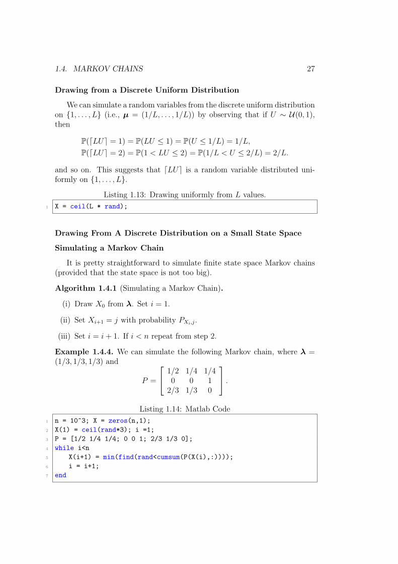
Drawing from a Discrete Uniform Distribution
We can simulate a random variables from the discrete uniform distributionon 1, . . . , L (i.e., µ = (1/L, . . . , 1/L)) by observing that if U ∼ U(0, 1),then
P(⌈LU⌉ = 1) = P(LU ≤ 1) = P(U ≤ 1/L) = 1/L,
P(⌈LU⌉ = 2) = P(1 < LU ≤ 2) = P(1/L < U ≤ 2/L) = 2/L.
and so on. This suggests that ⌈LU⌉ is a random variable distributed uni-formly on 1, . . . , L.
Listing 1.13: Drawing uniformly from L values.
1 X = ceil(L * rand);
Drawing From A Discrete Distribution on a Small State Space
Simulating a Markov Chain
It is pretty straightforward to simulate finite state space Markov chains(provided that the state space is not too big).
Algorithm 1.4.1 (Simulating a Markov Chain).
(i) Draw X0 from λ. Set i = 1.
(ii) Set Xi+1 = j with probability PXi,j.
(iii) Set i = i+ 1. If i < n repeat from step 2.
Example 1.4.4. We can simulate the following Markov chain, where λ =(1/3, 1/3, 1/3) and
P =
1/2 1/4 1/40 0 12/3 1/3 0
.
Listing 1.14: Matlab Code
1 n = 10^3; X = zeros(n,1);
2 X(1) = ceil(rand*3); i =1;
3 P = [1/2 1/4 1/4; 0 0 1; 2/3 1/3 0];
4 while i<n
5 X(i+1) = min(find(rand<cumsum(P(X(i),:))));
6 i = i+1;
7 end
28 CHAPTER 1. RANDOM WALKS ETC.
Unfortunately, in the case of Markov chains with big (or infinite) statespaces, this approach does not work. However, there is often another wayto simulate such Markov chains. We have already seen one such example forrandom walks.
1.4.2 Communication
It is very often the case that the distribution of Xn settles down to somefixed value as n grows large. We saw this in example 1.4.2. In order totalk about limiting behavior (and stationary distributions, which are closelyrelated) we need the transition matrix to posses certain properties. For thisreason, we introduce a number of definitions. We say that state i leads to
state j, written i → j, if
Pi(Xn = j for some n ≥ 0) > 0.
That is, if it is possible to get to j from i (though not necessarily in a singlestep). Assuming that λi > 0, Pi(A) = P(A |X0 = i). If no λ is specified,then assume that λi = 1.
Definition 1.4.5 (Communication). We say two states i, j ∈ X communi-
cate, denoted i ↔ j, if i → j and j → i.
Obviously, communicating is reflexive. That is, i → i for all i ∈ X . Wecan partition the state space X into communicating classes as follows. Wesay i and j are in the communicating class C if they communicate.
Example 1.4.6 (Communicating Classes). Consider the Markov chain withthe following graphical representation.
PICTURE HERE
There are two communicating classes C1 = 1, 2 and C2 = 3. In full, wehave the following relationships. 1 ↔ 2, 1 → 3 and 2 → 3.
Definition 1.4.7 (Irreducibility). We say a transition matrix P is irreducibleif X is a single communicating class (if it is always possible to get from onestate to another, though not always in just 1 step).
1.4.3 The Strong Markov Property
An important and (slightly) stronger property than the normal Markovproperty is the strong Markov property. To introduce this, we give our firstdefinition of a stopping time.

1.4. MARKOV CHAINS 29
Definition 1.4.8 (Stopping Time: Discrete Time Version). A random vari-able τ → 0, 1, ...∪∞ is a stopping time if the event τ = n only dependson X0, X1, . . . , Xn, for n ≥ 0.
Basically, in order for something to be a stopping time, we have to decideit has happen or not without knowing the future. So, for example τ =infn ≥ 0 : Xn = 1 is a stopping time, because we can tell when it occurswithout seeing into the future. On the other hand, τ = supn ≥ 0 : Xn = 1is not a stopping time for a random walk (we cannot tell when it happensunless we know the future). Another example of something that is not astopping time is τ = infn ≥ 0 : Xn+1 = i.
A stopping time that we have already encountered was the first passagetime for the random walk.
Theorem 1.4.9 (Strong Markov Property). Let Xnn≥0 be a (λ, P ) Markovchain and let τ be a stopping time of Xnn≥0. Then, conditional on τ < ∞and Xτ = i, Xτ+nn≥0 is a (δi, P ) Markov chain (δi is a distribution with 1at state i and 0 everywhere else) and is independent of X0, X1, . . . , Xτ .
Proof. See [3] for a proof.
1.4.4 Recurrence and Transience
All states in a Markov chain have the property of being either recurrentor transient.
Definition 1.4.10 (Recurrent). Given a Markov chain Xnn≥0 with tran-sition matrix P , we say that a state i is recurrent if
Pi(Xn = i for infinitely many n) = 1.
Definition 1.4.11 (Transient). Given a Markov chain Xnn≥0 with tran-sition matrix P , we say that a state i is transient if
Pi(Xn = i for infinitely many n) = 0.
In order to establish some important facts about recurrence and tran-sience, we need the following result about expectations of non-negative inte-ger valued random variables (random variables taking values in the naturalnumbers).
Theorem 1.4.12. Given a random variable X taking values in N,
EX =∞∑
i=0
P(X > i).

30 CHAPTER 1. RANDOM WALKS ETC.
Proof. We have
EX =∞∑
x=1
xP(X = x) =∞∑
x=1
x−1∑
i=0
P(X = x)
=∞∑
i=0
∞∑
x=i+1
P(X = x) =∞∑
i=0
P(X > i),
where we can swap sums because of the non-negative summands.
We also need to introduce a few stopping times.
Definition 1.4.13 (First Passage Time Including Return). We define thefirst passage time into the state i (including the possibility of starting in i)as
τi = infn ≥ 1 : Xn = i
Definition 1.4.14 (rth Passage Time). We define the rth passage time by
τ(0)i = 0 and
τ(r+1)i = infn < τ
(r)i : Xn = i for r ≥ 0.
We also define a sequence of random variables that are not stopping timesbut describe the times between visits to state i.
Definition 1.4.15 (rth Excursion Length). We define the rth excursionlength as
S(r)i =
τ(r)i − τ
(r−1)i if τ
(r−1)i < ∞
0 otherwise.
Lemma 1.4.16. For r ≥ 2, conditional on τ(r−1)i < ∞, S
(r)i is independent
of Xnτ(r−1)i
n≥0 and
P(S(r)i = n | τ (r−1)
i < ∞) = Pi(τi = n).
Proof. If we use the strong Markov property with the stopping time τ =τ(r−1)i , we get that Xτ+nn≥0 is a (δi, P ) Markov property that is indepen-
dent of X0, . . . , Xτ . Now, we can write S(r)i as
S(r)i = infn > 0 : Xτ+n = i,
so S(r)i is the first passage time, including return, to state i for Xτ+nn≥0.

1.4. MARKOV CHAINS 31
We define the number of visits to state i by
Vi =∞∑
n=0
I(Xn = i).
Let Ei be the expectation given that the process starts in state i.
Lemma 1.4.17. It holds that EiVi =∑∞
n=0 Pni,i.
Proof.
EiVi = Ei
∞∑
n=0
I(Xn = i) =∞∑
n=0
EiI(Xn = i) =∞∑
n=0
Pi(Xn = i) =∞∑
n=0
P ni,i.
Lemma 1.4.18. For r ≥ 0, Pi(Vi > r) = (Pi(τi < ∞))r .
Proof. When r = 0, this is clearly true. If it is true for r, then
Pi(Vi > r + 1) = Pi(τ(r+1)i < ∞) = Pi(τ
(r)i < ∞ and S
(r+1)i < ∞)
= Pi(S(r+1)i < ∞| τ (r)i < ∞)Pi(τ
(r)i < ∞) = Pi(τi < ∞)Pi(τ
(r)i < ∞).
Theorem 1.4.19. The following holds
(i) If Pi(τi < ∞) = 1 then i is recurrent and∑∞
n=0 Pni,i = ∞.
(ii) If Pi(τi < ∞) < 1 then i is transient and∑∞
n=0 Pni,i < ∞.
Proof. We prove the two statements separately.
Part 1. If Pi(τi < ∞) = 1 then Pi(Vi = ∞) = limr→∞ Pi(Vi > r). By lemma1.4.18,
limr→∞
Pi(Vi > r) = limr→∞
(Pi(τi < ∞))r = 1,
so i is recurrent. If Pi(Vi = ∞) = 1 then EiVi = ∞. Now, by lemma 1.4.17,
∞∑
n=0
P ni,i = EiVi = ∞.
32 CHAPTER 1. RANDOM WALKS ETC.
Part 2. If Pi(τi < ∞) < 1 then
Pi(Vi = ∞) = limr→∞
Pi(Vi > r) = limr→∞
(Pi(τi < ∞))r = 0,
so i is transient. Now,
∞∑
n=0
P ni,i = EiVi =
∞∑
r=0
Pi(Vi > r) =∞∑
r=0
(Pi(τi < ∞))r =1
1− Pi(τ < ∞)< ∞.
Theorem 1.4.20. Let C be a communicating class. Then either all statesin C are transient or all are recurrent.
Proof. Take a pair of states i and j in C and assume i is transient. Becausei and j are in the same communicating class, there must exist n ≥ 0 andm ≥ 0 so that P n
i,j > 0 and Pmj,i > 0. Now, it must be the case that
P n+r+mi,i ≥ P n
i,jPrj,jP
mj,i
as this only describes the probability of one possible path from i back to i(such a path need not pass through j). Rearranging, we have
P rj,j ≤
P n+r+mi,i
P ni,jP
mj,i
.
Summing over r we get
∞∑
r=0
P rj,j ≤
∑∞r=0 P
n+r+mi,i
P ni,jP
mj,i
.
Now, because i is assumed to be transient,∑∞
r=0 Pn+r+mi,i < ∞. As a result,∑∞
r=0 Prj,j < ∞, implying j is also transient. Thus, the only way a state can
be recurrent is if all states are recurrent.
Definition 1.4.21 (Closed Class). A communicating class C is closed ifi ∈ C and i → j implies j ∈ C.
Theorem 1.4.22. Every finite closed class is recurrent.
Proof. See [3].
As an irreducible Markov chain consists of one single closed class, thisimplies that all irreducible Markov chains on finite state spaces are recurrent.

1.4. MARKOV CHAINS 33
Recurrence of Random Walks
We can use the criteria given in theorem 1.4.19 to establish facts aboutthe recurrence properties of random walks. In order to establish recurrence,we would need
∑∞n=0 P
n0,0 = ∞. Thus, a first step is to find an expression
for P n0,0. As we have already discussed, a random walk starting at 0 can only
return to 0 in an even number of steps. Thus, it is sufficient for us to considerP 2n0,0. Now in order for a random walk to end up at 0 after 2n steps, it needs
to take exactly n up steps and n down steps. There are(2nn
)ways of taking
this many steps. This gives
P 2n0,0 =
(2n
n
)pn(1− p)n.
Lemma 1.4.23. The following bounds on n! hold of n ≥ 1.√2π nn+1/2 e−n ≤ n! ≤ e nn+1/2 e−n
Given these bounds on n! it is relatively straightforward to get boundson P n
0,0 that allow us to establish the transience or recurrence of the randomwalk.
Theorem 1.4.24. A symmetric random walk (i.e., a random walk withp = (1− p) = 1/2) is recurrent.
Proof. To show the random walk is recurrent, we need to show∞∑
n=0
P 2n0,0 = ∞.
The first step is to get a bound on(2nn
). By lemma 1.4.23, we have
(2n
n
)=
(2n)!
n!n!≥
√2π 2n2n+1/2 e−2n
e nn+1/2 e−ne nn+1/2 e−n=
2√π4n
e2√n.
So, we can bound the probabilities from below by
P 2n0,0 ≥
2√π
e2(4p(1− p))n√
n.
This implies that∞∑
n=0
P 2n0,0 ≥
2√π
e2
∞∑
n=0
(4p(1− p))n√n
.
If p = (1− p) then 4p(1− p) = 1, so∞∑
n=0
P 2n0,0 ≥ C
∞∑
n=0
1√n= ∞,
where C > 0 is a constant.

34 CHAPTER 1. RANDOM WALKS ETC.
1.4.5 Invariant Distributions
A topic of enormous interest, especially from a simulation perspective, isthe behavior of the distribution of a Markov chain, Xnn≥0 as n becomeslarge. It turns out there are actually a few different things we can mean bythis. The best possible situation is that a Markov chain can have a limiting
distribution. That is, there can exist a distribution, π, such that Xnn≥0 →π as n → ∞ no matter what initial distribution, λ, we choose. We willdiscuss the conditions for a limiting distribution to exist later. It turns out,however, that even if a limiting distribution does not exist, the Markov chainmay have a unique stationary distribution, sometimes also called an invariant
distribution or an equilibrium distribution. This is a distribution, π, such thatπP = π.
Definition 1.4.25 (Stationary Distribution). An invariant distribution of aMarkov chain with transition matrix P is a distribution that satisfies
πP = π.
The importance of stationary distributions is made clear by the followinglemma.
Lemma 1.4.26. Let Xnn≥0 be Markov (π, P ) and suppose π is a station-ary distribution for P , then Xn ∼ π for all n ≥ 0.
Proof. The distribution of Xn is given by πP n. Now, for n = 0 (where wedefine P 0 = I) it is clearly true that πP n = π. We just need to showπP n = π for n > 1. We do this by induction. That is, assume πP n = π.Then
πP n+1 = (πP )P n = πP n = π
by assumption. Thus, as this is true for n = 0, the result follows.
The obvious questions to ask when faced with a nice and interesting objectlike a stationary distribution are: does one exist? and, if so, is it unique?.The simple answer is that it is often the case that there is a unique stationarydistribution (at least for many of the Markov chains we might be interestedin), but that a number of conditions need to be fulfilled. One of these ispositive recurrence.
Recurrent implies that if the Markov chain starts in state i it will returnto state i with probability 1. However, this is no guarantee that the expectedreturn time is finite. Recall that mi = Eiτi, where τi = infn > 0 : Xn = i.Definition 1.4.27 (Positive Recurrence). We say a Markov chain is positiverecurrent if mi < ∞.
1.4. MARKOV CHAINS 35
Definition 1.4.28 (Null Recurrence). We say a Markov chain is null recur-rent if mi = ∞.
It is straightforward to establish that if a Markov chain is irreducible andhas a finite state space (i.e. |X | < ∞), then every state is positive recurrent.It is not always easy to show that an infinite state space Markov chain hassuch a property.
Now that we have defined positive recurrence, we are able to give condi-tions that guarantee a Markov chain has a unique stationary distribution.
Theorem 1.4.29. Let P be irreducible. Then the following are equivalent:
(i) Every state is positive recurrent.
(ii) Some state i is positive recurrent.
(iii) P has a (unique) invariant distribution, π, and mi = 1/πi.
Proof. See [3].
Note that it is possible for a Markov chain to have a stationary distribu-tion but not satisfy these conditions.
Example 1.4.30 (Calculating a stationary distribution). We can find a sta-tionary distribution by solving πP = π. For example, consider the followingMarkov chain
P =
0 1/2 1/21/2 0 1/21/2 1/2 0
.
So, we need to solve
(π1, π2, π2)
0 1/2 1/21/2 0 1/21/2 1/2 0
= (π1, π2, π2). (1.3)
This gives the following linear system
1
2π2 +
1
2π3 = π1
1
2π1 +
1
2π3 = π2
1
2π1 +
1
2π2 = π3.
Solving this, we have π1 = π2 = π3. As we need π1 + π2 + π3 = 1 if π is tobe a distribution, we have π1 = π2 = π3 = 1/3.

36 CHAPTER 1. RANDOM WALKS ETC.
1.4.6 Limiting Distribution
The fact that a Markov chain has a unique stationary distribution doesnot guarantee that it has a limiting distribution. This can be shown using asimple example.
Example 1.4.31 (A Markov chain with a stationary distribution but nolimiting distribution). Consider the Markov chain with graph
PICTURE HERE.
The transition matrix is given by
[0 11 0
]
This chain is clearly irreducible and positive recurrent, so it has a uniquestationary distribution, π = (1/2, 1/2). However, P 2n = I and P 2n+1 = P .This means that if we start with certainty in a given state the distributionwill not converge. For example, if λ = δi = (1, 0), then limn→∞ λP 2n = (1, 0)and limn→∞ λP 2n+1 = (0, 1). Thus, no limit exists.
The problem with the Markov chain in example 1.4.31 is that it is pe-riodic: it is only possible to get from state 1 back to state 1 in an evennumber of steps. In order for a Markov chain to have a limiting distribution,it should not have any periodicity. Unsurprisingly, this requirement is calledaperiodicity.
Definition 1.4.32. A state is said to be aperiodic if P ni,i > 0 for all sufficiently
large n. Equivalently, the set n ≥ 0 : P ni,i > 0 has no common divisor other
than 1.
In a irreducible Markov chain, all states are either aperiodic or periodic.
Theorem 1.4.33. Suppose P is irreducible and has an aperiodic state i.Then, all states are aperiodic.
A random walk is periodic with period 2.
Example 1.4.34.PICTURE HERE.
PICTURE HERE.
If a Markov chain is irreducible, positive recurrent and aperiodic, then ithas a limiting distribution.

1.4. MARKOV CHAINS 37
Theorem 1.4.35. Let P be irreducible and aperiodic and suppose P has aninvariant distribution π. Let λ be any distribution. and suppose Xnn≥0
is Markov (λ, P ). Then, P(Xn = j) → πj as n → ∞ for all j ∈ X . Inparticular, P n
i,j → πj as n → ∞ for all i, j ∈ X .
Proof. See [3].
1.4.7 Reversibility
Stationary distributions play a number of very important roles in simula-tion. In particular, we often wish to create a Markov chain that has a spec-ified stationary distribution. One important tool for finding such a Markovchain is to exploit a property called reversibility. Not all Markov chains arereversible but, as we shall see, those that are have some nice properties.
Definition 1.4.36. Let Xnn≥0 be a Markov (π, P ) with P irreducible. Wesay that Xnn≥0 is reversible if, for all N ≥ 1, XN−nNn=0 is also Markov(π, P ).
The most important property of reversible Markov chains is that theysatisfy the detailed balance equations.
Definition 1.4.37. A matrix P and a measure ν (a vector will all non-negative components) are in detailed balance if
νiPi,j = νjPj,i ∀i, j ∈ X .
The detailed balance equations are important because they allow us tofind stationary distributions (and, as we will learn later, construct transitionmatrices with given stationary distributions).
Lemma 1.4.38. If P and the distribution π are in detailed balance, then π
is invariant for P .
Proof. We have
(πP )i =∑
j∈X
πjPj,i =∑
j∈X
πiPi,j = πi.
The following theorem shows that reversibility is equivalent to satisfyingthe detailed balance equations.
38 CHAPTER 1. RANDOM WALKS ETC.
Theorem 1.4.39. Let P be an irreducible stochastic matrix and let π bea distribution. Suppose Xnn≥0 is Markov (π, P ). Then, the following areequivalent.
(i) Xnn≥0 is reversible.
(ii) P and π are in detailed balance (i.e., π is the stationary distributionof P ).
Proof. See [3].
Random Walks on Graphs
Given a graph with a finite number of vertices, labeled 1, . . . , L, each withfinite degree (i.e., d1 < ∞, . . . , dL < ∞), we can define a random walk withthe following transition probabilities
Pi,j =
1di
if there is an edge between i and j
0 otherwise.
Example 1.4.40 (A random walk on a graph). Consider the following graph.
PICTURE HERE.
Using the above transition probabilities, we have the Markov chain
PICTURE HERE.
If a graph is connected, then a random walk on it will be irreducible.Given a connected graph, it is easy to establish the stationary distributionof the resulting random walk using the detailed balance equations.
Lemma 1.4.41. For connected graphs with∑
i di < ∞ we have
πi =di∑i∈X di
.
Proof. We just need to confirm that the detailed balance equations hold andthat the probabilities sum to 1. First, observe that
di∑i∈X di
1
di=
dj∑i∈X dj
1
djholds for all i, j ∈ X .
Now, pretty clearly,∑
i∈X πi = 1, so we are done.
1.4. MARKOV CHAINS 39
Example 1.4.42 (A random walk on a graph (cont.)). For the graph givenin example 1.4.40, we have
d1 + d2 + d3 + d4 = 2 + 3 + 3 + 2 = 10.
Thus,π1 = 2/10, π2 = 3/10, π3 = 3/10, π4 = 2/10.
1.4.8 The Ergodic Theorem
The ergodic theorem is something like the strong law of large numbersfor Markov chains. It tells us the sample averages converge to expectedvalues almost surely. In addition, the second part of the theorem is veryuseful practically as it is often the case that we are not directly interestedin a Markov chain, Xnn≥0, but rather in the behavior of some stochasticprocess Ynn≥0, where Yn = f(Xn) and f is a deterministic function. Forexample Xnn≥0 could be a Markov chain describing the weather and fcould be a function describing how much electricity is consumed by a town(on average) under certain weather conditions. We might then be interestedin the average power consumption, which we could estimate by the sampleaverage
Sn =1
n
n∑
k=0
f(Xk).
The ergodic theorem guarantees that such sample averages converge to thecorrect expected values.
Definition 1.4.43 (Number of visits to i before time n). We define thenumber of visits to i before time n by
Vi(n) =n−1∑
k=0
I(Xk = i).
Theorem 1.4.44 (Ergodic Theorem). Let Xnn≥0 be Markov (λ, P ), whereP is an irreducible transition matrix and λ is an arbitrary initial distribution.Then,
P
(Vi(n)
n→ 1
mi
as n → ∞)
= 1.
If, in addition, P is positive recurrent, then for any bounded function f :X → R,
P
(1
n
n−1∑
k=0
f(Xk) →∑
i∈X
πif(i) as n → ∞)
= 1,
where π is the stationary distribution of P .
40 CHAPTER 1. RANDOM WALKS ETC.
Proof.
Part 1. If P is transient, then the chain will only return to state i a finitenumber of times. This means that
Vi(n)
n≤ Vi
n→ 0 =
1
mi
.
Now, consider the recurrent case. For a given state i, we have P(τi < ∞) = 1.Using the strong Markov property, the Markov chain Xτi+nn≥0 is Markov(δi, P ) and independent of X0, . . . , Xτi . As the long run proportion of timespend in i is the same for Xnn≥0 and Xτi+nn≥0, we are safe to assumethat the chain starts in i.
Now, by time n − 1, the chain will have made at most V (n) visits to i.It will certainly have made at least V (n)− 1 visits. The total length of timerequired to make all these visits must be less than or equal to n−1 (because,by definition, all these visits occur within the first n− 1 steps). This meansthat
S(1)i + · · ·+ S
(Vi(n)−1)i ≤ n− 1.
By a similar argument,
n ≤ S(1)i + · · ·+ S
(Vi(n))i .
Using these bounds, we have
S(1)i + · · ·+ S
(Vi(n)−1)i
Vi(n)≤ n
Vi(n)≤ S
(1)i + · · ·+ S
(Vi(n))i
Vi(n).
Now, we know the the excursion lengths are i.i.d. random variables (withfinite mean mi), so, by the large of large numbers,
P
(S(1)i + · · ·+ S
(n)i
n→ mi as n → ∞
)= 1.
Now, we know that P(Vi(n) → ∞ as n → ∞) = 1. So, letting n → ∞, wesqueeze n/Vi(n) to get
P
(n
Vi(n)→ mi as n → ∞
)= 1.
This implies that
P
(Vi(n)
n→ 1
mi
as n → ∞)
= 1.
Part 2. See [3].
1.5. EXTENDING THE RANDOM WALK MODEL 41
1.5 Extending the Random Walk Model
1.5.1 Sums of Independent Random Variables
If we consider a random walk with x0 = 0, we can define it by
Xn =n∑
i=1
Zi,
where the Zii≥1 are i.i.d. random variables with
P(Z1 = 1) = 1− P(Z1 = −1) = p.
If we replace the Zii≥1 with an arbitrary sequence of independent ran-dom variables, Yii≥1 we are in the setting of sums of independent randomvariables. That is, we consider
Sn =n∑
i=1
Yi.
Now, in the case of a random walk, which is a sum of the Zii≥1 randomvariables, we know the distribution of Sn (we calculated this earlier). How-ever, this is not always the case. Normally, in order to find the distributionof a sum of n random variables, we have to calculate an n-fold convolution oruse either moment generating functions or characteristic functions and hopethat things work out nicely.
Recall, given two independent random variables, X and Y , the convolu-tion of the distributions of X and Y is given by
P(X + Y = z) =∞∑
x=−∞
P(X = x)P(Y = z − x)
=∞∑
y=−∞
P(X = z − y)P(Y = y)
in the discrete case and the convolution, h, of the density of X, f , and thedensity of Y , g, is given by
h(z) = (f ∗ g)(z) =∫ ∞
−∞
f(x)g(z − x)dx =
∫ ∞
−∞
f(z − y)g(y)dy
in the continuous case. It is easy to see that the calculations can be prettymessy if lots of variables with different distributions are involved.

42 CHAPTER 1. RANDOM WALKS ETC.
Sometimes, things are nice. For example, the sum of independent normalrandom variables is normally distributed and the sum of i.i.d. exponentialrandom variables is distributed according to a special case of the gammadistribution (called the Erlang distribution). But most things are not sonice. For example, try to work out the distribution of n exponential randomvariables with parameters λ1, . . . , λn.
There are various tools in mathematics that help us deal with sums ofindependent random variables. For example, we have the Lindeberg centrallimit theorem and a version of the strong law of large numbers. However,these do not answer all the questions we might reasonably ask and there arelots of random variables that do not satisfy the technical conditions of thesetheorems. Simulation is a useful tool for solving problems in these settings.
We will consider a couple of examples that use normal random variables.Recall that if Z ∼ N(0, 1) then X = µ+ σZ ∼ N(µ, σ2). This means we cansimulate a normal random variable with mean µ and variance σ2 in Matlabusing the command
X = mu + sqrt(sigma_sqr) * randn;
Another new concept in the examples is relative error.
Definition 1.5.1 (Relative Error). The relative error of an estimator ℓ isdefined by
RE =
√Var(ℓ)
ℓ.
Basically, the relative error tell us the size of our estimator’s error as apercentage of the thing we are tying to estimate (i.e., if we have a relativeerror of 0.01, that means that the standard deviation of our estimator isabout 1 percent of ℓ). The relative error is often a more meaningful measureof error in settings where the thing we are trying to estimate, ℓ, is small. Inpractice, the relative error needs to be estimated.
Example 1.5.2 (Sums of log-normal random variables). Consider a port-folio consisting of n stocks (which, for some reason, are independent of oneanother). At the start of the year, the stocks all have value 1. The changes invalue of these stocks over a year are given by the random variables V1, . . . , Vn,which are log-normal random variables, i.e., V1 = eZ1 , ., Vn = eZn withZ1 ∼ N(µ1, σ
21), · · · , Z1 ∼ N(µn, σ
2n). It is not so straightforward to calculate
the distribution of Sn = V1 + · · ·+ Vn.If n = 5, with µ = (−0.1, 0.2,−0.3, 0.1, 0) and σ2 = (0.3, 0.3, 0.3, 0.2, 0.2),
what is the probability that the portfolio is worth more than 20 at the

1.5. EXTENDING THE RANDOM WALK MODEL 43
end of the year? It is straightforward to use Monte Carlo to get an es-timate of ℓ = P(Sn > 20). Here, we check that the mean and varianceof our simulation output correspond to the theoretical mean and variance(it never hurts to check things seem to be working properly). The meanof a log-normal random variable is given by expµ + σ2/2 and the vari-ance is given by (expσ2 − 1)exp2µ + σ2. In addition, we estimateE [max(V1, . . . , V5) |S5 > 20] (that is, the average value of the largest portfoliocomponent when the portfolio has a value bigger than 20) and E [S5 |S5 > 20].
Listing 1.15: Matlab code
1 N = 5*10^7; S = zeros(N,1); threshold = 20;
2 V_max = zeros(N,1); V_mean = zeros(N,1);
3
4 mu = [-0.1 0.2 -0.3 0.1 0]; sigma_sqr = [.3 .3 .3 .2 .2];
5
6 for i = 1:N
7 Z = mu + sqrt(sigma_sqr) .* randn(1,5);
8 V = exp(Z);
9 V_max(i) = max(V);
10 S(i) = sum(V);
11 end
12
13 est_mean = mean(S)
14 actual_mean = sum(exp(mu + sigma_sqr/2))
15
16 est_var = var(S)
17 actual_var = sum((exp(sigma_sqr) - 1) .* exp(2 * mu + sigma_sqr))
18
19 ell_est = mean(S>threshold)
20 ell_RE = std(S>threshold) / (ell_est * sqrt(N))
21
22 [event_occurs_index dummy_var] = find(S > threshold);
23 avg_max_v = mean(V_max(event_occurs_index))
24 avg_S = mean(S(event_occurs_index))
Running this one time produced the following output
est_mean = 5.6576
actual_mean = 5.6576
est_var = 1.9500
actual_var = 1.9511
ell_est = 2.3800e-06
ell_RE = 0.0917
44 CHAPTER 1. RANDOM WALKS ETC.
avg_max_v = 15.9229
avg_S = 21.5756
Notice that, on average, the rare event seems to be caused by a singleportfolio component taking a very large value (rather than all the portfoliocomponents taking larger than usual values). This is typical of a class ofrandom variables called heavy tailed random variables, of which the log-normal distribution is an example.
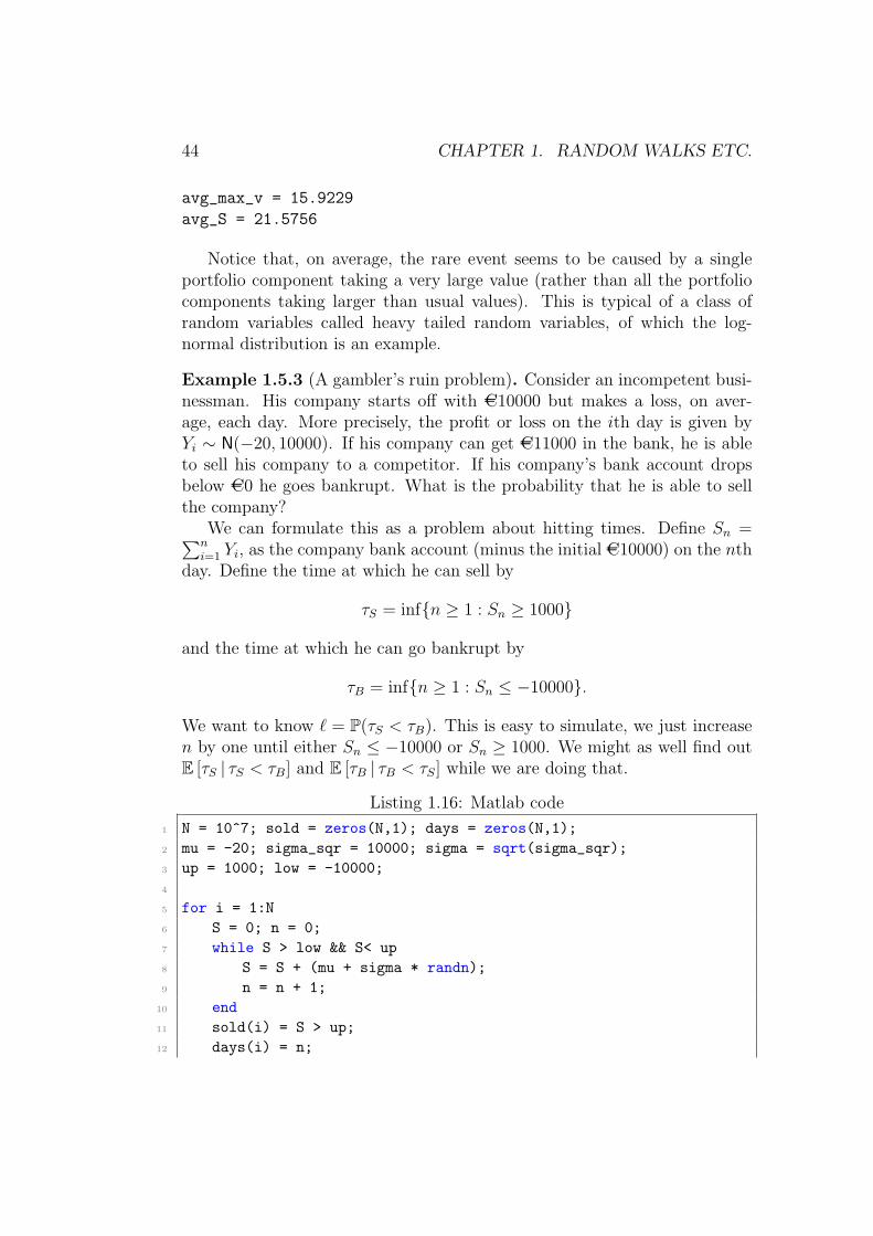
Example 1.5.3 (A gambler’s ruin problem). Consider an incompetent busi-nessman. His company starts off with AC10000 but makes a loss, on aver-age, each day. More precisely, the profit or loss on the ith day is given byYi ∼ N(−20, 10000). If his company can get AC11000 in the bank, he is ableto sell his company to a competitor. If his company’s bank account dropsbelow AC0 he goes bankrupt. What is the probability that he is able to sellthe company?
We can formulate this as a problem about hitting times. Define Sn =∑ni=1 Yi, as the company bank account (minus the initial AC10000) on the nth
day. Define the time at which he can sell by
τS = infn ≥ 1 : Sn ≥ 1000
and the time at which he can go bankrupt by
τB = infn ≥ 1 : Sn ≤ −10000.
We want to know ℓ = P(τS < τB). This is easy to simulate, we just increasen by one until either Sn ≤ −10000 or Sn ≥ 1000. We might as well find outE [τS | τS < τB] and E [τB | τB < τS] while we are doing that.
Listing 1.16: Matlab code
1 N = 10^7; sold = zeros(N,1); days = zeros(N,1);
2 mu = -20; sigma_sqr = 10000; sigma = sqrt(sigma_sqr);
3 up = 1000; low = -10000;
4
5 for i = 1:N
6 S = 0; n = 0;
7 while S > low && S< up
8 S = S + (mu + sigma * randn);
9 n = n + 1;
10 end
11 sold(i) = S > up;
12 days(i) = n;

1.6. IMPORTANCE SAMPLING 45
13 end
14
15 ell_est = mean(sold)
16 est_RE = sqrt(sold) / (sqrt(N)*ell_est)
17
18 [event_occurs_index dummy_var] = find(sold == 1);
19 [event_does_not_occur_index dummy_var] = find(sold == 0);
20
21 avg_days_if_sold = mean(days(event_occurs_index))
22 avg_days_if_bankrupt = mean(days(event_does_not_occur_index))
Running this one time produced the following output
ell_est = 0.0145
ell_RE = 0.0026
avg_days_if_sold = 52.9701
avg_days_if_bankrupt = 501.5879
1.6 Importance Sampling
In examples 1.5.2 and 1.5.3, the probabilities we were interested in werequite small. Estimating such quantities is usually difficult. If you think aboutit, if something only happens on average once every 106 times, then you willneed a pretty big sample size to get many occurrences of that event. We canbe a bit more precise about this. Consider the relative error of the estimatorℓ for ℓ = P(X > γ) = EI(X > γ). This is of the form
RE =
√P(X > γ) (1− P(X > γ))
P(X > γ)√N
.
So, for a fixed RE, we need
√N =
√P(X > γ) (1− P(X > γ))
P(X > γ)RE⇒ N =
1− P(X > γ)
P(X > γ)RE2 .
So N = O(1/P(X > γ)) which means N gets big very quickly as ℓ = P(X >γ) → 0. This is a big problem in areas where events with small probabilitiesare important. There are lots of fields where such events are important: forexample, physics, finance, telecommunication, nuclear engineering, chemistryand biology. One of the most effective methods of estimating these probabil-ities is called importance sampling.

46 CHAPTER 1. RANDOM WALKS ETC.
In the case of sums of independent random variables, the basic idea isto change the distributions of the random variables so that the event we areinterested in is more likely to occur. Of course, if we do this, we will have abiased estimator. So, we need a way to correct for this bias. It is easiest todescribe these things using continuous random variables and densities but, aswe will see in the examples, everything works for discrete random variablesas well.
Consider a random variable X taking values in R with density f . Supposewe wish to estimate ℓ = ES(X). Note that we can write
ES(X) =
∫ ∞
−∞
S(x) f(x) dx.
Now, this suggests the natural estimator
ℓ =1
N
N∑
i=1
S(X(i)),
where X(1), . . . , X(N) are i.i.d. draws from the density f . Now, supposethe expectation of S(X) is most influenced by a subset of values with lowprobability. For example, if S(X) = I(X > γ) and P(X > γ) is small,then this set of values would be x ∈ X : S(x) > γ. We want to find away to make this ‘important’ set of values happen more often. This is theidea of importance sampling. The idea is to sample X(i)Ni=1 according toanother density, g, that ascribes much higher probability to the importantset. Observe that, given a density g such that g(x) = 0 ⇒ f(x)S(x) = 0,and being explicit about the density used to calculate the expectation,
EfS(X) =
∫ ∞
−∞
S(x) f(x) dx =
∫ ∞
−∞
S(x)g(x)
g(x)f(x) dx
=
∫ ∞
−∞
S(x)f(x)
g(x)g(x) dx = Eg
f(X)
g(X)S(X).
We call f(x)/g(x) the likelihood ratio. This suggests, immediately, the im-portance sampling estimator
Definition 1.6.1 (The Importance Sampling Estimator). The importance
sampling estimator, ℓIS, of ℓ = ES(X) is given by
ℓIS =1
N
N∑
i=1
f(X(i))
g(X(i))S(X(i)),
where the X(i)Ni=1 are i.i.d. draws from the importance sampling densityg.
1.6. IMPORTANCE SAMPLING 47
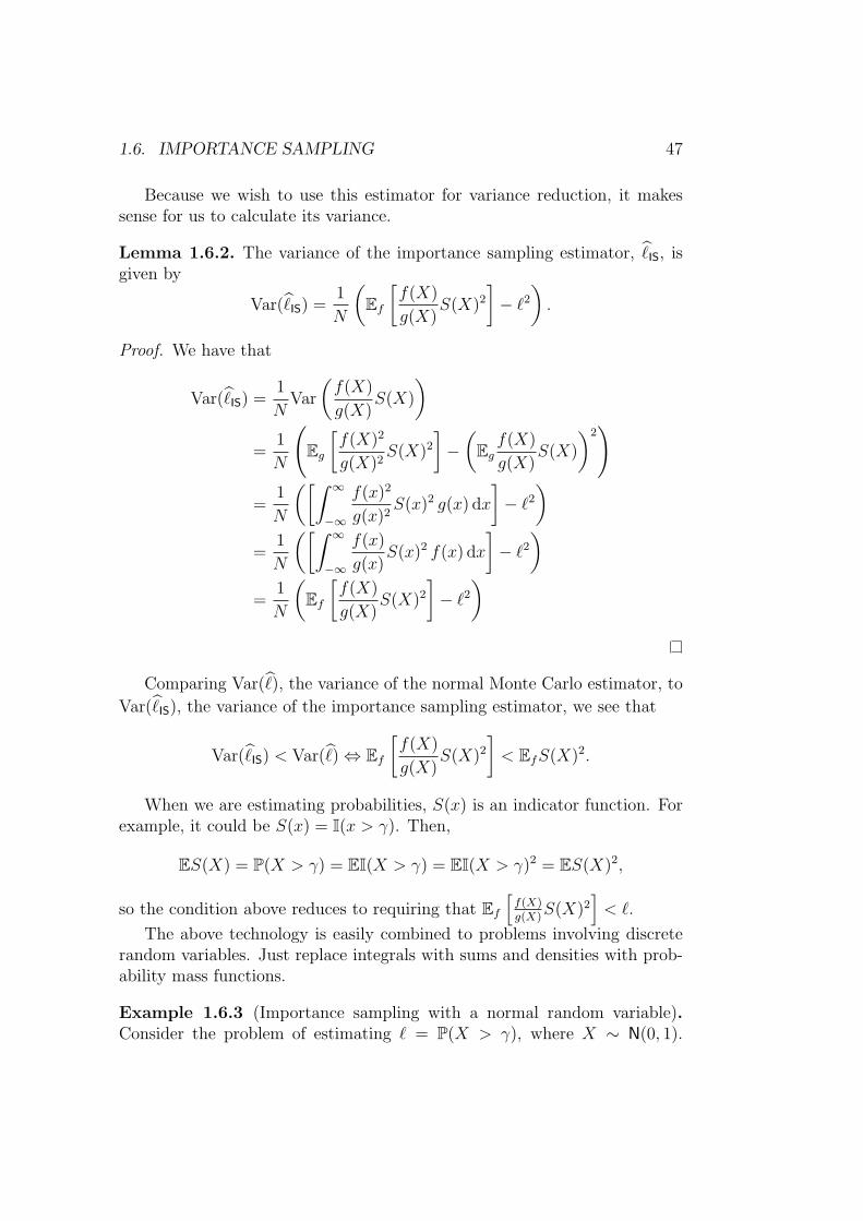
Because we wish to use this estimator for variance reduction, it makessense for us to calculate its variance.
Lemma 1.6.2. The variance of the importance sampling estimator, ℓIS, isgiven by
Var(ℓIS) =1
N
(Ef
[f(X)
g(X)S(X)2
]− ℓ2
).
Proof. We have that
Var(ℓIS) =1
NVar
(f(X)
g(X)S(X)
)
=1
N
(Eg
[f(X)2
g(X)2S(X)2
]−(Eg
f(X)
g(X)S(X)
)2)
=1
N
([∫ ∞
−∞
f(x)2
g(x)2S(x)2 g(x) dx
]− ℓ2
)
=1
N
([∫ ∞
−∞
f(x)
g(x)S(x)2 f(x) dx
]− ℓ2
)
=1
N
(Ef
[f(X)
g(X)S(X)2
]− ℓ2
)
Comparing Var(ℓ), the variance of the normal Monte Carlo estimator, to
Var(ℓIS), the variance of the importance sampling estimator, we see that
Var(ℓIS) < Var(ℓ) ⇔ Ef
[f(X)
g(X)S(X)2
]< EfS(X)2.
When we are estimating probabilities, S(x) is an indicator function. Forexample, it could be S(x) = I(x > γ). Then,
ES(X) = P(X > γ) = EI(X > γ) = EI(X > γ)2 = ES(X)2,
so the condition above reduces to requiring that Ef
[f(X)g(X)
S(X)2]< ℓ.
The above technology is easily combined to problems involving discreterandom variables. Just replace integrals with sums and densities with prob-ability mass functions.
Example 1.6.3 (Importance sampling with a normal random variable).Consider the problem of estimating ℓ = P(X > γ), where X ∼ N(0, 1).

48 CHAPTER 1. RANDOM WALKS ETC.
If γ is big, for example γ = 5, then ℓ is very small. The standard estimatorof ℓ = P(X > γ) is
ℓ =1
N
N∑
i=1
I(X(i) > γ
),
where the X(i)Ni=1 are i.i.d. N(0, 1) random variables. This is not a goodestimator for large γ. We can code this as follows.
Listing 1.17: Matlab code
1 gamma = 5; N = 10^7;
2 X = randn(N,1);
3 ell_est = mean(X > gamma)
4 RE_est = std(X > gamma) / (sqrt(N) * ell_est)
For γ = 5 with a sample size of 107, an estimate of the probability is 2×10⁻⁷
and an estimate of the relative error is 0.7071. So, this problem is a goodcandidate for importance sampling. An obvious choice of an importancesampling density is a normal density with variance 1 but with mean γ. Thelikelihood ratio f(x)/g(x) is given by
f(x)
g(x)=
(√2π)−1
exp−12x2
(√2π)−1
exp−12(x− γ)2
= exp
γ2
2− xγ
.
Thus, the estimator will be of the form
ℓIS =1
N
N∑
i=1
exp
γ2
2−X(i)γ
I(X(i) > γ
),
where the X(i)Ni=1 are i.i.d. N(γ, 1) random variables. The code for thisfollows.
Listing 1.18: Matlab code
1 gamma = 5; N = 10^7;
2 X = gamma + randn(N,1);
3 values = exp(gamma^2 / 2 - X*gamma) .* (X > gamma);
4 ell_est = mean(values)
5 RE_est = std(values) / (sqrt(N) * ell_est)
For γ = 5 with a sample size of 107 an estimate of the probability is 2.87×10⁻⁷
and an estimate of the relative error is 7.53 × 10⁻⁴. We can check the truevalue in this case using the Matlab command
1 - normcdf(5)

1.6. IMPORTANCE SAMPLING 49
This gives a value of 2.87× 10⁻⁷ which is more or less identical to the valuereturned by our estimator.
If we have a sum of n independent variables, X1, . . . , Xn, with densitiesf1, . . . , fn, we can apply importance sampling using densities g1, . . . , gn. Wewould then have a likelihood ratio of the form
n∏
i=1
fi(x)
gi(x).
Everything then proceeds as before.
Example 1.6.4 (A rare event for a random walk). Given a random walk,Xnn≥0, with x0 = 0 and p = 0.4, what is ℓ = P(X50 > 15)? We canestimate this in Matlab using standard Monte Carlo.
Listing 1.19: Matlab code
1 N = 10^5; threshold = 15;
2 n = 50; p = 0.4; X_0 = 0;
3 X_50 = zeros(N,1);
4
5 for i = 1:N
6 X = X_0;
7 for j = 1:n
8 Y = rand <= p;
9 X = X + 2*Y - 1;
10 end
11 X_50(i) = X;
12 end
13 ell_est = mean(X_50 > threshold)
14 RE_est = std(X_50 > threshold) / (sqrt(N) * ell_est)
Running this program once, we get an estimated probability of 1.2×10⁻⁴
and an estimated relative error of 0.29. This is not so great, so we can tryusing importance sampling. A good first try might be to simulate a randomwalk, as before, but with another parameter, q = 0.65. If we write
Xn =n∑
i=1
Zi,
then, the original random walk is simulated by generating the Zii≥1 ac-cording to the probability mass function p I(Z = 1) + (1 − p) I(Z = −1).Generating the new random walk means generating the Zii≥1 according to

50 CHAPTER 1. RANDOM WALKS ETC.
the probability mass function q I(Z = 1)+(1−q) I(Z = −1). This then givesa likelihood ratio of the form
n∏
i=1
p I(Zi = 1) + (1− p) I(Zi = −1)
q I(Zi = 1) + (1− q) I(Zi = −1)=
n∏
i=1
[p
qI(Zi = 1) +
1− p
1− qI(Zi = −1)
].
We can implement the estimator in Matlab as follows.
Listing 1.20: Matlab code
1 N = 10^5; threshold = 15;
2 n = 50; p = 0.4; X_0 = 0; q = 0.65;
3 X_50 = zeros(N,1); LRs = zeros(N,1);
4
5 for i = 1:N
6 X = X_0; LR = 1;
7 for j = 1:n
8 Y = rand <= q;
9 LR = LR * (p/q * (Y == 1) + (1-p) / (1 - q) * (Y == 0));
10 X = X + 2*Y - 1;
11 end
12 LRs(i) = LR;
13 X_50(i) = X;
14 end
15 ell_est = mean(LRs .* (X_50 > threshold))
16 RE_est = std(LRs .* (X_50 > threshold)) / (sqrt(N) * ell_est)
Running this program, we get an estimated probability of 1.81× 10⁻⁴ and arelative error of 0.0059. We can check this makes sense by using the standardMonte Carlo estimator with a much bigger sample size. Using a sample sizeof N = 108, we get an estimate of 1.81 × 10⁻⁴, confirming the importancesampling gives the right result.
Rules of Thumb for Effective Importance Sampling
Recall the definition of a moment generating function.
Definition 1.6.5 (Moment Generating Function). We define the momentgenerating function of a random variable X by
M(θ) = EeθX .
For θ = 0, M(θ) = 1. However, for other values of θ, it may not bethe case that M(θ) < ∞. In order for M(θ) to be finite for some θ 6=0, the probability of X taking very large (or small) values has to go to

1.6. IMPORTANCE SAMPLING 51
zero exponentially fast. This leads to the definition of light-tailed randomvariables. Usually, people assume that light-tailed means right light-tailed.
Definition 1.6.6 (Light-tailed random variable). We say a random variableX is (right) light-tailed if M(θ) < ∞ for some θ > 0. We say X is leftlight-tailed if M(θ) < ∞ for some θ < 0.
The rules of thumb, which only apply when dealing with light-tailed ran-dom variables, are as follows.
• For sums of i.i.d. random variables, e.g., P(X1 + · · ·+Xn > γ) choosethe importance sampling density, g, so that EgX1 = γ/n.
• For stopping time problems, e.g., P(τA < τB) or P(τA < ∞), wherethe process is drifting away from A, the set of interest, choose g sothat the drift of the stochastic process is reversed. For example, ifA = 10, 11, . . . and Sn =
∑ni=1 Yi, with Yi ∼ N(−1, 1), then choose g
so that EgZ1 = 1.
1.6.1 Weighted Importance Sampling
If is often the case that we wish to estimate ℓ = EfS(X) without knowingeverything about the density f . For example, a density can be written as
f(x) =h(x)
Z,
where Z is the normalizing constant (that is Z =∫h(x) dx). In many
realistic applications, we do not know Z, even if we do know h and have away of sampling from f (it is often possible to sample from a density withoutknowing its normalizing constant). An obvious problem, then, is how weshould carry out importance sampling in such a setting.
Weighted importance sampling is one way of addressing this problem. Thenormal importance sampling estimator is of the form
ℓIS =1
N
N∑
i=1
f(X(i))
g(X(i))S(X(i)),
where X(1), . . . ,X(N) is an i.i.d. sample from g. This returns a sample meanthat is weighted by the likelihood ratios
f(X(1))
g(X(1)), . . . ,
f(X(N))
g(X(N)).

52 CHAPTER 1. RANDOM WALKS ETC.
The idea of weighted importance sampling is to use another weight, which isof the form
W (x) =h(x)
g(x).
Instead of using the standard importance sampling estimator, we now haveto use an estimator of the form
ℓWIS =1N
∑Ni=1 W
(X(i)
)S(X(i)
)
1N
∑Ni=1 W (X(i))
,
with X(1), . . . ,X(N) an i.i.d. sample from g.Now,
EgW (X)S(X) = Egh(X)
g(X)S(X) =
∫h(x)
g(x)S(x)g(x) dx
= Z
∫h(x)
ZS(x) dx = Z EfS(X).
Likewise,
EgW (X) = Egh(X)
g(X)=
∫h(x)
g(x)g(x) dx = Z
∫h(x)
Zdx = Z.
Thus, by the strong law of large numbers, we get in the limit that
limN→∞
1N
∑Ni=1 W
(X(i)
)S(X(i)
)
1N
∑Ni=1 W (X(i))
→ Z EfS(X)
Z= EfS(X).
Note that this estimator is biased. However, the bias is O(1/n), so it is nottoo bad in practice (and we don’t always have an alternative).
1.6.2 Sequential Importance Sampling
So far, when we have considered a problem like ℓ = P(X10 > 5), we haveconsidered a process that can be written as a sum of independent randomvariables. For example
Xn =n∑
i=1
Yi,
where Y1, . . . , Yn are i.i.d. draws from f . In this case, we can write
ℓIS =1
N
N∑
i=1
(10∏
j=1
f(Y(i)j )
g(Y(i)j )
)I
(10∑
j=1
Y(i)j > 5
).

1.6. IMPORTANCE SAMPLING 53
One advantage of this formulation is that if we can sample Y1, calculatethe likelihood ratio, then sample Y2, update the likelihood ratio (by multi-plying by f(Y2)/g(Y2)), and so on. In particular, if we wish to simulate aprocess until a stopping time, then we can simply stop when this stoppingtime is reached, without having to worry about how to calculate the jointdensity afterwards. When the Yjnj=1 are dependent, things are a little morecomplicated. Continuing with our ℓ = P(X10 > 5) example, in the case ofdependent random variables, we would write
ℓIS =1
N
N∑
i=1
f(Y(i)1 , . . . , Y
(i)n )
g(Y(i)1 , . . . , Y
(i)n )
I
(10∑
j=1
Y(i)j > 5
).
However, we can often write this in a more convenient form. Note that,
f(y1, . . . , yn) = f(y1)f(y2 | y1) · · · f(yn | y1, . . . , yn−1),
or, in Bayesian notation (which makes things a bit more compact),
f(y1:n) = f(y1)f(y2 | y1) · · · f(yn | y1:n−1)
Likewise, we can write
g(y1:n) = g(y1)g(y2 | y1) · · · g(yn | y1:n−1).
If we know these conditional densities, then we can write the likelihood ratioin the form
Wn(y1:n) =f(y1)f(y2 | y1) · · · f(yn | y1:n−1)
g(y1)g(y2 | y1) · · · g(yn | y1:n−1).
If we write,
W1(y1) =f(y1)
g(y1),
then
W2(y1:2) =f(y2 | y1)g(y2 | y1)
f(y1)
g(y1)=
f(y2 | y1)g(y2 | y1)
W1(y1),
and, more generally,
Wn(y1:n) =f(yn | y1:n−1)
g(yn | y1:n−1)Wn−1(y1:n−1).
In cases where the Markov property holds,
Wn(y1:n) =f(yn | yn−1)
g(yn | yn−1)Wn−1(y1:n−1).
Using this formulation, we can update until a stopping time, then stop up-dating. This formulation also allows for sophisticated methods, such as thosewere certain low probability paths (i.e., paths with very small weights) arerandomly killed.

54 CHAPTER 1. RANDOM WALKS ETC.
1.6.3 Self-Avoiding Random Walks
Consider a random walk on a 2d lattice. That is, a Markov chain,Xnn≥0, on Z× Z with X0 = 0 and transition probabilities given by
P (Xn = (k, l) |Xn−1 = (i, j)) =
1/4 , if |k − i|+ |l − j| = 1
0 , otherwise.
Self-avoiding random walks are simply random walks that do not hitthemselves.
−5 −4 −3 −2 −1 0 1 2 3 4 5−5
−4
−3
−2
−1
0
1
2
3
4
5
−5 −4 −3 −2 −1 0 1 2 3 4 5−5
−4
−3
−2
−1
0
1
2
3
4
5
Figure 1.6.1: Two realizations of a self-avoiding random walk with 7 steps.
−10 −8 −6 −4 −2 0 2 4 6 8 10−10
−8
−6
−4
−2
0
2
4
6
8
10
−10 −8 −6 −4 −2 0 2 4 6 8 10−10
−8
−6
−4
−2
0
2
4
6
8
10
Figure 1.6.2: Two realizations of a self-avoiding random walk with 20 steps.
Self avoiding walks are useful as simple models of objects like polymers.They capture some fundamental behavior of strings of molecules that cannotbe too close to one another, but otherwise have minimal interaction. Theyalso appear in mathematical objects like random graphs and percolationclusters.
It is easy to generate a self-avoiding random walk of length n via MonteCarlo if n is small. We simply simulate random walks of length n until oneof them is self-avoiding.
Listing 1.21: Matlab code

1.6. IMPORTANCE SAMPLING 55
1 n = 7; i = 1;
2
3 while(i ~= n)
4 X = 0; Y = 0;
5 lattice = zeros(2*n + 1, 2*n+1);
6 lattice(n+1, n+1) = 1;
7 path = [0 0];
8 for i = 1:n
9
10 U = rand;
11 if U < 1/2
12 X = X + 2 * (U < 1/4) - 1;
13 else
14 Y = Y + 2 * (U < 3/4) - 1;
15 end
16
17 path_addition = [X Y];
18 path = [path; path_addition];
19
20 lattice_x = n + 1 + X;
21 lattice_y = n + 1 + Y;
22
23 if lattice(lattice_x, lattice_y) == 1
24 i = 1; break;
25 else
26 lattice(lattice_x, lattice_y) = 1;
27 end
28 end
29 end
30
31 clf; hold on;
32 axis([-n n -n n]);
33 for j = 1:n
34 line([path(j,1), path(j+1,1)], [path(j,2), path(j+1,2)]);
35 end
The problem is that for large n, it is very unlikely that a random walkwill be a self-avoiding random walk. To put this in perspective, there are 4n
possible random walks of length n on the 2D square lattice. In general, thenumber of self-avoiding random walks for a given n is not known. However,for small n, these have been calculated.
• For n = 5, there are 284 self-avoiding walks. So, the probability that a

56 CHAPTER 1. RANDOM WALKS ETC.
single random walk of length 5 will be self-avoiding is
284
45=
284
1024≈ 0.2773.
This means we only need to generate roughly 4 walks in order to get aself-avoiding one.
• For n = 10, there are 441000 self-avoiding random walks. So, theprobability is
44100
410=
44100
1048576≈ 0.0421.
This means we need to generate about 24 walks in order to get a self-avoiding one.
• For n = 20, there are 897697164 self-avoiding random walks. Theprobability is
897697164
420≈ 8.16× 10⁻⁴.
so we need to generate about 1125 walks in order to get a self-avoidingone.
Pretty clearly, the situation becomes unworkable by n = 100 or n = 150.Unfortunately, people are often interested in asymptotic results when con-sidering objects like self-avoiding random walks. In order to get informationabout asymptotic behavior, we need to be able to generate statistics for ran-dom walks with large n values. An obvious modification to the standardalgorithm would be to try to choose the next step of the random walk toavoid the places the random walk has already been. The simplest way todo this is to chose the next site of the random walk from the set of emptyneighbors of the current site.
PICTURE HERE
This approach is straightforward to implement in Matlab.
Listing 1.22: Matlab code
1 n = 250; i = 1;
2 moves = [0 1; 0 -1; -1 0; 1 0];
3
4 while(i ~= n)
5 X = 0; Y = 0;
6 lattice = zeros(2*(n+1) + 1, 2*(n+1)+1);
7 lattice(n+2, n+2) = 1;
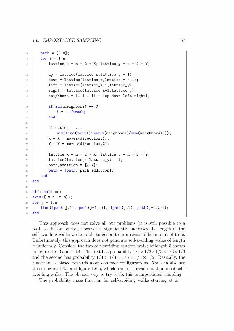
1.6. IMPORTANCE SAMPLING 57
8 path = [0 0];
9 for i = 1:n
10 lattice_x = n + 2 + X; lattice_y = n + 2 + Y;
11
12 up = lattice(lattice_x,lattice_y + 1);
13 down = lattice(lattice_x,lattice_y - 1);
14 left = lattice(lattice_x-1,lattice_y);
15 right = lattice(lattice_x+1,lattice_y);
16 neighbors = [1 1 1 1] - [up down left right];
17
18 if sum(neighbors) == 0
19 i = 1; break;
20 end
21
22 direction = ...
23 min(find(rand<(cumsum(neighbors)/sum(neighbors))));
24 X = X + moves(direction,1);
25 Y = Y + moves(direction,2);
26
27 lattice_x = n + 2 + X; lattice_y = n + 2 + Y;
28 lattice(lattice_x,lattice_y) = 1;
29 path_addition = [X Y];
30 path = [path; path_addition];
31 end
32 end
33
34 clf; hold on;
35 axis([-n n -n n]);
36 for j = 1:n
37 line([path(j,1), path(j+1,1)], [path(j,2), path(j+1,2)]);
38 end
This approach does not solve all our problems (it is still possible to apath to die out early), however it significantly increases the length of theself-avoiding walks we are able to generate in a reasonable amount of time.Unfortunately, this approach does not generate self-avoiding walks of lengthn uniformly. Consider the two self-avoiding random walks of length 5 shownin figures 1.6.3 and 1.6.4. The first has probability 1/4×1/3×1/3×1/3×1/3and the second has probability 1/4 × 1/3 × 1/3 × 1/3 × 1/2. Basically, thealgorithm is biased towards more compact configurations. You can also seethis in figure 1.6.5 and figure 1.6.5, which are less spread out than most self-avoiding walks. The obvious way to try to fix this is importance sampling.
The probability mass function for self-avoiding walks starting at x0 =

58 CHAPTER 1. RANDOM WALKS ETC.
Figure 1.6.3: A path of a self-avoiding walk of length 5.
Figure 1.6.4: A path of a self-avoiding walk of length 5.
−30 −25 −20 −15 −10 −5 0 5
−30
−25
−20
−15
−10
−5
0
5
Figure 1.6.5: A realization of a self-avoiding random walk with 250 stepsusing the new technique.

1.6. IMPORTANCE SAMPLING 59
−10 −5 0 5 10 15 20 25 30
−20
−15
−10
−5
0
5
10
Figure 1.6.6: A realization of a self-avoiding random walk with 250 stepsusing the new technique.
(x0, y0), which we represent by x1 = (x1, y1), . . . ,xn = (xn, yn), is given by
p(x1, . . . ,xn) =I ((x1, . . . ,xn) ∈ En)
Zn
,
where En is the set of self-avoiding random walks of length n. Unfortunately,as mentioned before, we do not know Zn. However, we can use weightedimportance sampling instead. To do this, we still need an expression forq(x1, . . . ,xn), the probability mass function based on the new method. Wecan get this expression using sequential importance sampling. Note that, atstep i−1 of the random walk, we know all the information up to step i−1, sowe can calculate q(xi |x0, . . . ,xi−1). Let di−1 be the number of unoccupiedneighbors of xi−1. This is a function of x0, . . . ,xi−1. Then,
q(xi |x0, . . . ,xi−1) =
1/di−1, if xi is an unoccupied neighbor of xi−1
0, otherwise
Thus, a successful realization of a self-avoiding random walk under our algo-rithm, x1, . . . ,xn will have a probability of
q(x1, . . . ,xn) =I ((x1, . . . ,xn) ∈ En)
d0 · · · dn−1
Note that p(x1, . . . ,xn) ∝ I ((x1, . . . ,xn) ∈ En), so we can use weights of theform
W (x1, . . . ,xn) = I ((x1, . . . ,xn) ∈ En) d0 · · · dn−1,
in weighted importance sampling.
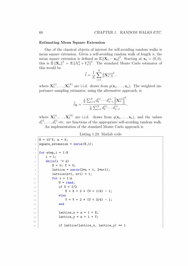
60 CHAPTER 1. RANDOM WALKS ETC.
Estimating Mean Square Extension
One of the classical objects of interest for self-avoiding random walks ismean square extension. Given a self-avoiding random walk of length n, themean square extension is defined as E ‖Xn − x0‖2. Starting at x0 = (0, 0),this is E ‖Xn‖2 = E ‖X2
n + Y 2n ‖
2. The standard Monte Carlo estimator of
this would be
ℓ =1
N
N∑
i=1
∥∥X(i)n
∥∥2 ,
where X(1)n , . . . ,X
(N)n are i.i.d. draws from p(x1, . . . ,xn). The weighted im-
portance sampling estimator, using the alternative approach, is
ℓIS =
1N
∑Ni=1 d
(i)0 · · · d(i)n−1
∥∥∥X(i)n
∥∥∥2
1N
∑Ni=1 d
(i)0 · · · d(i)n−1
,
where X(1)n , . . . ,X
(N)n are i.i.d. draws from q(x1, . . . ,xn), and the values
d(i)1 , . . . , d
(i)n etc. are functions of the appropriate self-avoiding random walk.
An implementation of the standard Monte Carlo approach is
Listing 1.23: Matlab code
1 N = 10^5; n = 5;
2 square_extension = zeros(N,1);
3
4 for step_i = 1:N
5 i = 1;
6 while(i ~= n)
7 X = 0; Y = 0;
8 lattice = zeros(2*n + 1, 2*n+1);
9 lattice(n+1, n+1) = 1;
10 for i = 1:n
11 U = rand;
12 if U < 1/2
13 X = X + 2 * (U < 1/4) - 1;
14 else
15 Y = Y + 2 * (U < 3/4) - 1;
16 end
17
18 lattice_x = n + 1 + X;
19 lattice_y = n + 1 + Y;
20
21 if lattice(lattice_x, lattice_y) == 1

1.6. IMPORTANCE SAMPLING 61
22 i = 1;
23 break;
24 else
25 lattice(lattice_x, lattice_y) = 1;
26 end
27 end
28 end
29
30 square_extension(step_i) = X^2 + Y^2;
31 end
32
33 mean_square_extension = mean(square_extension)
An implementation of the importance sampling version is
Listing 1.24: Matlab code
1 N = 10^5; n = 150; square_extension = zeros(N,1);
2 moves = [0 1; 0 -1; -1 0; 1 0];
3
4 for step_i = 1:N
5 i = 1;
6 while(i ~= n)
7 X = 0; Y = 0; weight = 1;
8 lattice = zeros(2*(n+1) + 1, 2*(n+1)+1);
9 lattice(n+2, n+2) = 1;
10 for i = 1:n
11 lattice_x = n + 2 + X; lattice_y = n + 2 + Y;
12 up = lattice(lattice_x,lattice_y + 1);
13 down = lattice(lattice_x,lattice_y - 1);
14 left = lattice(lattice_x-1,lattice_y);
15 right = lattice(lattice_x+1,lattice_y);
16 neighbors = [1 1 1 1] - [up down left right];
17
18 if sum(neighbors) == 0
19 i = 1; break;
20 end
21 weight = weight * sum(neighbors);
22 direction = ...
23 min(find(rand<(cumsum(neighbors)/sum(neighbors))));
24 X = X + moves(direction,1);
25 Y = Y + moves(direction,2);
26 lattice_x = n + 2 + X; lattice_y = n + 2 + Y;
27 lattice(lattice_x,lattice_y) = 1;
28 end

62 CHAPTER 1. RANDOM WALKS ETC.
29 end
30 weights(step_i) = weight;
31 square_extension(step_i) = X^2 + Y^2;
32 end
33 mean_square_extension = ...
34 mean(weights’.*square_extension) / mean(weights)

Chapter 2
Poisson Processes andContinuous Time MarkovChains
2.1 Stochastic Processes in Continuous Time
In order to discuss stochastic processes in continuous time, we need toupdate a few of the definitions we have been working with.
Technically, a stochastic process lives on a probability space (Ω,F ,P).Typical choices of Ω are C[0,∞), the space of all continuous functions on[0,∞), and D[0,∞), the space of right continuous left limit (cadlag) func-tions. An element, ω, of Ω is then a function. We can then define a stochasticprocess by Xt(ω) = ω(t). We often take F to be the smallest σ-algebra suchthat ω → ω(t) is measurable for each t ≥ 0. We usually work with a setof probability measures Pxx∈X , where Px is the probability measure of astochastic process starting at X0 = x (i.e., Px(X0 = x) = 1). I will use P
without a subscript to denote a stochastic process started at 0 (or sometimessomething else if the context is explicit enough).
A continuous time, general state space stochastic process takes values ina state space X that is equipped with an appropriate σ-algebra, Σ. Often,X will be R and Σ will then be B(R), the Borel σ-algebra on R.
The first thing we need is a way of rigorously talking about the historyof a process. In the discrete time case, we could simply consider X0, . . . , Xn.Now, we need something a bit more sophisticated, called a filtration.
Definition 2.1.1 (Filtration). A filtration Ftt≥0 is an increasing family ofsub σ-algebras of F (that is, Fs ⊆ Ft ⊆ F for all s ≤ t).
63

64 CHAPTER 2. POISSON PROCESSES AND CTMCS
We will require/assume that a filtration is right continuous. That is,
Ft =⋂
s≥t
Fs ∀t ≥ 0.
We need the filtration to contain some information about Xtt≥0 (other-wise, it is not very useful). We say Xtt≥0 is adapted to a filtration, Ftt≥0
if the filtration contains sufficient information about Xtt≥0. More formally,
Definition 2.1.2. A process, Xtt≥0 is adapted to a filtration Ftt≥0, orFt-adapted, if Xt is Ft measurable for all t ≥ 0.
We normally assume we are working the natural filtration of a process(augmented so that it is right-continuous).
Definition 2.1.3 (Natural Filtration). The natural filtration of a process,FX
t t≥0 is the filtration generated by the process itself. That is
FXt = σ(Xs : 0 ≤ s ≤ t).
If we augment the natural filtration by adding certain sets of measure zero,we will usually (in situations we consider) get a right-continuous filtration.When this is possible, we assume that by natural filtration we mean theaugmented natural filtration.
Equipped with the concept of a filtration, we can define stopping timesin continuous time.
Definition 2.1.4 (Stopping Time : Continuous Time Version). A randomvariable τ : Ω → [0,∞] is said to be a stopping time with respect to thefiltration Ftt≥0 if τ ≤ t ∈ Ft for all t ≥ 0.
We can also define a continuous time general state space version of theMarkov property.
Definition 2.1.5 (Markov Property: Continuous Time). We say an Ft-adapted stochastic process Xtt≥0 taking values in X has the Markov prop-erty if
Px(Xt+s ∈ A | Fs) = Px(Xt+s ∈ A |Xs) Px almost surely,
for all x ∈ X , 0 ≤ s ≤ t and A ∈ Σ.
Likewise, we can define a continuous time version of the strong Markovproperty.

2.2. THE POISSON PROCESS 65
Definition 2.1.6 (Strong Markov Property: Continuous Time). We say anFt-adapted stochastic process Xtt≥0 taking values in X has the strongMarkov property if, given a stopping time τ and conditional on τ < ∞,
Px(Xt+τ ∈ A | Fτ ) = Px(Xt+τ ∈ A |Xτ ) Px almost surely,
for all x ∈ X , 0 ≤ s ≤ t and A ∈ Σ.
2.2 The Poisson Process
The Poisson process is one of the fundamental stochastic processes inprobability. We can use it to build many complex and interesting stochasticobjects. It is a very simple model for processes such as the arrival of people ina queue, the number of cars arriving at a red traffic light, and the occurrenceof insurance claims.
2.2.1 Point Processes on [0,∞)
A Poisson process is a point process on [0,∞). We will not considersuch point processes in their most general form, but rather a straightforwardand easy to work with subset of point processes. We can use a number ofequivalent definitions. The first of these is to see the point process in termsof a counting process. A counting process, Ntt≥0 counts the number ofevents that have happened by time t.
Definition 2.2.1 (Point Process on [0,∞): Counting Process Version). Apoint process on [0,∞) is a process Ntt∈[0,∞) taking values in N that:
(i) Vanishes at 0. That is, N0− = N0 = 0, where Nt− = limu↑t Nu.
(ii) Is non-decreasing. That is, N0 ≤ Ns ≤ Nt for 0 ≤ s ≤ t.
(iii) Is right continuous. That is, Nt = Nt+ , where Nt+ = limu↓t Nu.
(iv) Has unit jumps. That is, Nt −Nt− ∈ 0, 1. Technically, a process whereonly one jump can occur at a given time t is called a simple point
process.
(v) Has an infinite limit. That is, limt→∞ Nt = ∞.
Note, again, that some of these requirements can be relaxed.

66 CHAPTER 2. POISSON PROCESSES AND CTMCS
Definition 2.2.2 (Point Process on [0,∞): Jump Instances Version). Apoint process on [0,∞) is defined by a sequence Tnn≥1 of random variablesthat are positive and increasing to infinity. That is,
0 < T1 < T2 < · · · < ∞ and limn→∞
Tn = ∞.
This defines the counting process
Nt =∑
n≥1
I(Tn ≤ t) = supn ≥ 1 : Tn ≤ t.
Definition 2.2.3 (Point Process on [0,∞): Inter-arrivals Version). A pointprocess on [0,∞) is defined by a sequence Snn≥1 of positive random vari-ables such that
∑n≥1 Sn = ∞. These define a sequence of jump instances by
S1 = T1 and Sn = Tn − Tn−1 for n ≥ 2.
PICTURE HERE
These three definitions of point processes suggest three possible ways tosimulate them.
(i) We can simulate the counting process Ntt≥0 (or its increments).
(ii) We can simulate the jump times Tnn≥1.
(iii) We can simulate the inter-arrival times Snn≥1.
The key properties of a Poisson process (aside from being a point process)are that it has stationary increments and independent increments.
Definition 2.2.4 (Stationary Increments). A stochastic process Xtt≥0 hasstationary increments if the distribution of Xt+h −Xt depends only on h forh ≥ 0.
Definition 2.2.5 (Independent Increments). A stochastic process Xtt≥0
has independent increments if the random variables Xti+1− Xtini=1 are
independent whenever 0 ≤ t1 < t2 < · · · < tn and n ≥ 1.
A process that has stationary and independent increments is attractivefrom a simulation perspective because we can simulate it in ’parts’ (the in-crements).
2.2. THE POISSON PROCESS 67
2.2.2 Poisson Process
Equipped with the necessary definitions, we can now define a Poissonprocess.
Definition 2.2.6 (Poisson Process on [0,∞)). A (homogenous) Poisson pro-cess on [0,∞) with parameter λ > 0 is a point process on [0,∞) with sta-tionary and independent increments and Nt ∼ Poi(λt) for all t ≥ 0. Thatis,
P(Nt = k) = e−λt (λt)k
k!.
Actually, we can define a Poisson process in a number of different ways.
Theorem 2.2.7 (Poisson process). The following definitions are equivalentdefinitions.
(i) A Poisson process is a point process, Ntt≥0, with stationary andindependent increments with Nt ∼ Poi(λt) for all t ≥ 0.
(ii) A Poisson process is a point process, Ntt≥0, with independent incre-ments and the property that, as h ↓ 0, uniformly in t
(a) P(Nt+h −Nt = 0) = 1− λh+ o(h).
(b) P(Nt+h −Nt = 1) = λh+ o(h).
(c) P(Nt+h −Nt > 1) = o(h).
(iii) A Poisson process is a point process defined by its inter-arrival times,Snn≥1, which are i.i.d. Exp(λ).
Before we prove anything, we need a few results.
Lemma 2.2.8 (Memoryless Property). We say that exponential randomvariables have the memoryless property. That is, for t, s ≥ 0, if X ∼ Exp(λ),then
P(X > t+ s |X > s) = P(X > t).
Proof. We can write P(X > t+ s |X > s) as
P(X > t+ s,X > s)
P(X > s).
As s < t then P(X > t+ s,X > s) = P(X > t), so
P(X > t+ s,X > s)
P(X > s)=
P(X > t+ s)
P(X > s)=
e−λ(t+s)
e−λs= e−λ(t) = P(X > t).
68 CHAPTER 2. POISSON PROCESSES AND CTMCS
Theorem 2.2.9 (Markov Property). If Ntt≥0 is a Poisson process withrate λ > 0, then, for any s > 0, Nt+s−Nst≥0 is also a Poisson process withrate λ. Furthermore, this process is independent of Nrr≤s.
Proof. First, note that the event Ns = i can be written as
Ns = i = Ti ≤ s ∩ Si+1 > s− Ti
and, given this, for r ≤ s,
Nr =i∑
j=1
I(Sj ≤ r).
Define the process starting at time s by Nt = Nt+s − Ns. Then, givenNs = i, S1 = Si+1 − (s − Ti) and Sn = Si+n for n ≥ 2. Now, by the
memoryless property, S1 is an Exp(λ) random variable. Thus the Snn≥1 arei.i.d. Exp(λ) random variables independent of S1, . . . , Sn. Thus, conditional
of Ns = i, Ntt≥0 is a Poisson process independent of Xrr≤s.
Now, we can prove Theorem 2.2.7.
Proof. I give a number of proofs of equivalences here. The rest will be leftfor exercises or self-study.
Part 1. First, we will show that (i) implies (ii). Now, as the increments arestationary, we know Nt+h −Nt has the same distribution as Nh −N0. So,
P(Nt+h −Nt = 0) = P(Nh −N0 = 0) = P(Nh = 0) = e−λh.
Taking a Taylor expansion of the exponential function, we get e−λh = 1 −λh+ o(h). Likewise,
P(Nt+h −Nt = 1) = P(Nh = 1) = λhe−λh = λh+ o(h).
and P(Nt+h −Nt > 1) = o(h).
Part 2. We will show that (ii) implies (i). We do this by solving somedifferential equations. First, let us define pj(t) = P(Nt = j). Then,
p0(t+h) = P(Nt+h = 0) = P(Nt+h−Nt = 0)P(Nt = 0) = (1−λh+o(h))p0(t).
Rearranging, we have
p0(t+ h)− p0(t)
h= −λp0(t) +
o(h)
h.

2.2. THE POISSON PROCESS 69
Because this holds for all t, we also get
p0(t)− p0(t− h)
h= −λp0(t− h) +
o(h)
h.
Letting h → 0 shows that p0(t) has a derivative (as the limit exists). Thisgives us
p0(t)′ = −λp0(t) ⇒ p0(t) = Ae−λt.
Now, because N0 = 0, we know that p0(0) = 1 so A = 1 (i.e., p0(t) = e−λt).Doing the same for pj(t) we have
pj(t+ h) =
j∑
i=0
P(Nt+h −Nt = i)P(Nt = j − i)
= P(Nt+h −Nt = 0)P(Nt = j) + P(Nt+h −Nt = 1)P(Nt = j − 1)
+
j∑
i=2
P(Nt+h −Nt = i)P(Nt = j − i)
= (1− λh+ o(h))pj(t) + (λh+ o(h))pj−1(t) + o(h).
Rearranging, we have
pj(t+ h)− pj(t)
h= −λpj(t) + λpj−1(t) +
o(h)
h.
By a similar argument to the one above, we get
pj(t)′ = −λpj(t) + λpj−1(t).
Now, remember that the product rule tells us that (fg)′ = f ′g + g′f . If weuse the integrating factor eλt, we get
pj(t)′ = −λpj(t) + λpj−1(t) ⇒ eλtpj(t) = −λeλtpj(t) + λeλtpj−1(t)
⇒ eλtpj(t)′ + λeλtpj(t) = λeλtpj−1(t) ⇒
(eλtpj(t)
)′= λeλtpj−1(t).
We can solve this by induction. We start with j = 1. This gives(eλtp1(t)
)′= λeλtp0(t) = λeλte−λt = λ.
Integrating, we get
eλtp1(t) = λt+ A ⇒ p1(t) = tλeλt + Aeλt.
Now, pj(0) = 0 for j > 0, so A = 0 and p1(t) = tλeλt. Repeating in this way,we get
pj(t) = P(Nt = j) = e−λt (λt)j
j!.
70 CHAPTER 2. POISSON PROCESSES AND CTMCS
Part 3. We show that (iii) implies (ii). This is just like the proof that (i)implies (ii). Using the Markov property (which was based on the interarrivalsdefinition) we observe that Nt+h −Nt has the same distribution as Nh, so
P(Nt+h −Nt = 0) = P(Nh = 0) = P(S1 > h) = e−λh = 1− λh+ o(h),
and
P(Nt+h −Nt = 1) = P(Nh = 0) = P(S1 < h, S1 + S2 > h)
=
∫ h
0
e−λ(h−u)λe−λu du =
∫ h
0
λe−λh du = λhe−λh = λh+ o(h).
It is also straightforward to see that
P(Nt+h −Nt > 1) = P(S1 < h, S1 + S2 < h) ≤ P(S1 < h)P(S2 < h) = o(h).
2.2.3 Order Statistics and the Distribution of ArrivalTimes
Order Statistics
Consider identically distributed random variables X1, . . . , Xn with distri-bution F (x) (that is P(X < x) = F (x). The order statistics of these randomvariables are simply the random variables ordered from smallest to largest.We write these as X(1) ≤ X(2) ≤ . . . ≤ X(n). Two of the most importantorder statistics are the minimum, X(1), and the maximum, X(n).
Lemma 2.2.10. The distribution of the minimum is given by
P(X(1) ≤ x
)= 1− (1− F (x))n .
Proof. We have
P(X(1) ≤ x
)= 1− P
(X(1) > x
)= 1− P(X1 > x, . . . , Xn > x)
= 1− P(X1 > x) · · ·P(Xn > x) = 1− (P(X > x))n = 1− (1− F (x))n .
Lemma 2.2.11. The distribution of the maximum is given by
P(X(n) ≤ x
)= F (x)n

2.2. THE POISSON PROCESS 71
Proof. We have
P(X(n) ≤ x
)= P(X1 ≤ x, . . . , Xn ≤ x) = P(X ≤ x)n = F (x)n.
Lemma 2.2.12. The density of the order statistics of n random variablesU1, . . . , Un, with distribution U(a, b), is given by
f(u1, . . . , un) =n!
(b− a)nI(a ≤ u1 ≤ · · · ≤ un ≤ b)
Proof. It is easiest to begin with the distribution and then take derivativesto get the density. We wish to calculate P
(U(1) ≤ u1, . . . , U(n) ≤ un
). Note
that there are n! orderings of the uniform random variables, each of which isequally likely. So,
P(U(1) ≤ u1, . . . , U(n) ≤ un
)= n!P(U < u1) · · ·P(U < un)
= n!u1 − a
b− a· · · un − a
b− a.
Taking derivatives, we get
f(u1, . . . , un) =∂
∂u1
· · · ∂
∂un
P(U(1) ≤ u1, . . . , U(n) ≤ un
)
=n!
(b− a)nI(a ≤ u1 ≤ · · · ≤ un ≤ b).
Distribution of Arrival Times
As it turns out, given that we know how many arrivals a Poisson processhas had in an interval [0, t] (that is, we know Nt), the arrival times willbe uniformly distributed in the interval. This implies that the points of aPoisson process have very little structure to them (in some sense, it is aprocess that puts points as arbitrarily as possible on a line).
Theorem 2.2.13. Let Ntt≥0 be a Poisson process. Then, conditional onNt = n, T1, . . . , Tn have the joint density function
f(t1, . . . , tn) =n!
tnI(0 ≤ t1 ≤ · · · ≤ tn ≤ t).
This is the density of the order statistics of i.i.d. uniform random variableson the interval [0, t]. This means the arrival times are distributed uniformlyon this interval.

72 CHAPTER 2. POISSON PROCESSES AND CTMCS
Proof. Consider the event T1 = t1, . . . , Tn = tn, Nt = n. Because there is abijection between arrival times and inter-arrival times, this should have thesame probability density as the event
S1 = t1, S2 = t2 − t1, . . . , Sn = tn − tn−1, Sn+1 > t− tn.
Because this is the joint density of i.i.d. exponential random variables, wecan write this explicitly as
λe−λu1λe−λ(u2−u1) · · ·λe−λ(un−un−1)e−λ(t−un) = λne−λt.
We then get the conditional density we wish by dividing by the probabilityof the event Nt = n,
f(t1, . . . , tn) =λne−λt
(λt)ne−λt/n!I(0 ≤ t1 ≤ · · · ≤ tn ≤ t)
=n!
tnI(0 ≤ t1 ≤ · · · ≤ tn ≤ t).
2.2.4 Simulating Poisson Processes
As already mentioned, there are at least three ways of simulating a Pois-son process. These follow directly from the different definitions we have used.
Using the Infinitesimal Definition to Simulate Approximately
The infinitesimal definition gives us a way to simulate the counting pro-cess Ntt≥0 directly. This simulation is approximate but becomes increas-ingly good as h ↓ 0. The idea is to slice the interval [0, t] up into little piecesof length (sometimes called mesh size) h. In each one of these slices, weincrease Ntt≥0 with probability λh.
Listing 2.1: Matlab code
1 lambda = 4; t = 1; h = 0.0001;
2 mesh = 0:h:t; N = zeros(1, length(mesh));
3 S = []; jump_indices = [];
4
5 N(1) = 0;
6
7 for i = 2:length(mesh)
8 if rand < lambda * h

2.2. THE POISSON PROCESS 73
9 jump_indices = [jump_indices i];
10 N(i) = N(i-1) + 1;
11 else
12 N(i) = N(i-1);
13 end
14 end
15
16 if isempty(jump_indices)==0
17 Ts = (jump_indices - 1)*h;
18 S(1) = Ts(1);
19 if length(jump_indices) > 1
20 for i = 2:length(jump_indices)
21 S(i) = Ts(i) - Ts(i-1);
22 end
23 end
24 end
Simulating the Arrival Times
The idea of this approach is to simulate the arrival times directly. Givenan interval [0, t], we know that we have a Poi(λt) random number of arrivals.These are then distributed uniformly in [0, t].
Listing 2.2: Matlab code
1 t = 5; lambda = 2;
2
3 T = [];
4 n = poissrnd(lambda * t);
5
6 if n~=0
7 T = sort(t * rand(n,1));
8 S = zeros(n,1);
9 S(1) = T(1);
10 if n > 1
11 for i = 2:n
12 S(i) = T(i) - T(i-1);
13 end
14 end
15 end

74 CHAPTER 2. POISSON PROCESSES AND CTMCS
Simulating the Inter-Arrival Times
The idea here is to simulate the inter-arrival times, which are i.i.d. Exp(λ)random variables. Note that, if U ∼ U(0, 1), then − log(U)/λ is Exp(λ).
Listing 2.3: Matlab code
1 lambda = 4; h = 0.0001; t = 1;
2
3 s = 0;
4
5 S = []; Ts = [];
6
7 while s <= t
8 inter_time = - log(rand) / lambda;;
9 s = s + inter_time;
10 if s > t
11 break;
12 else
13 Ts = [Ts s];
14 S = [S inter_time];
15 end
16 end
2.2.5 Inhomogenous Poisson Processes
For many of the processes that Poisson processes are used to model, suchas queues and traffic, the assumption that events occur at a constant rate(i.e., λ is constant) is very unrealistic. If you think about traffic (either on theinternet or on a road) it tends to be heavier in some time periods and lighter inothers. Inhomogenous Poisson processes modify the definition of a Poissonprocess so that it can incorporate time-dependent arrivals. InhomogenousPoisson processes can be defined in a number of ways. Note, however, that itis no longer straightforward to use a definition based on inter-arrival times.
Definition 2.2.14 (Inhomogenous Poisson Process). A point process Ntt≥0
is said to be an inhomogenous Poisson process with intensity function λ(t) ≥0 ∀t ≥ 0.
(i) N0 = 0.
(ii) For each t ≥ 0, Nt has a Poisson distribution with paramater Λ =∫ t
0λ(s) ds.

2.2. THE POISSON PROCESS 75
(iii) For each 0 ≤ t1 < t2 < · · · < tm, the random variables Nt1 , . . . , Ntm −Ntm−1 are independent (that is, Ntt≥0 has independent increments).
Definition 2.2.15 (Inhomogenous Poisson Process (Infinitesimal Defini-tion)). A point process Ntt≥0 is said to be an inhomogenous Poisson processwith intensity function λ(t) ≥ 0∀t ≥ 0 if, as h ↓ 0,
(i) Ntt≥0 has independent increments.
(ii) P(Nt+h −Nt = 0) = 1− λ(t)h+ o(h).
(iii) P(Nt+h −Nt = 1) = λ(t)h+ o(h).
(iv) P(Nt+h −Nt > 1) = o(h).
2.2.6 Simulating an Inhomogenous Poisson Process
There are at least two ways to simulate an inhomogenous Poisson process.
Acceptance-Rejection
One way to simulate an inhomogenous Poisson process on an interval [0, t]is to simulate a homogenous Poisson process with parameter
λ∗ = maxλ(s) : 0 ≤ s ≤ t
then ‘thin’ this process by only accepting arrivals with a certain probability.If an arrival / jump occurs at time Ti it should only be accepted with prob-ability λ(T1)/λ
∗. It is not hard to check that this method works using theinfinitesimal definition.
Listing 2.4: Matlab code
1 t = 10; lambda_star = 1;
2
3 T = [];
4 n = poissrnd(lambda_star * t);
5
6 if n~=0
7 point_count = 0;
8 for i = 1:n
9 T_temp = t * rand;
10 if rand < sin(T_temp)^2 / lambda_star
11 point_count = point_count + 1;
12 T(point_count) = T_temp;

76 CHAPTER 2. POISSON PROCESSES AND CTMCS
13 end
14 end
15 if point_count ~= 0
16 T = sort(T);
17 S = zeros(point_count,1);
18 S(1) = T(1);
19 if point_count > 1
20 for i = 2:point_count
21 S(i) = T(i) - T(i-1);
22 end
23 end
24 end
25 end
Infinitesimal Approach (Approximate)
As in the homogenous Poisson process case, we can simulate an inho-mogenous Poisson process approximately using its infinitesimal definition.This approximation becomes better as h ↓ 0.
0 1 2 3 4 5 6 7 8 9 100
0.2
0.4
0.6
0.8
1
Figure 2.2.1: A realization of a inhomogenous Poisson process with the in-tensity function λ(t) = 3 sin2(t) plotted.
Listing 2.5: Matlab code
1 lambda = 1; t = 10; h = 0.0001;
2 mesh = 0:h:t; N = zeros(1, length(mesh));
3 S = []; jump_indices = [];
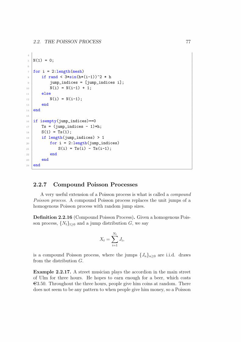
2.2. THE POISSON PROCESS 77
4
5 N(1) = 0;
6
7 for i = 2:length(mesh)
8 if rand < 3*sin(h*(i-1))^2 * h
9 jump_indices = [jump_indices i];
10 N(i) = N(i-1) + 1;
11 else
12 N(i) = N(i-1);
13 end
14 end
15
16 if isempty(jump_indices)==0
17 Ts = (jump_indices - 1)*h;
18 S(1) = Ts(1);
19 if length(jump_indices) > 1
20 for i = 2:length(jump_indices)
21 S(i) = Ts(i) - Ts(i-1);
22 end
23 end
24 end
2.2.7 Compound Poisson Processes
A very useful extension of a Poisson process is what is called a compound
Poisson process. A compound Poisson process replaces the unit jumps of ahomogenous Poisson process with random jump sizes.
Definition 2.2.16 (Compound Poisson Process). Given a homogenous Pois-son process, Ntt≥0 and a jump distribution G, we say
Xt =Nt∑
i=1
Ji,
is a compound Poisson process, where the jumps Jnn≥0 are i.i.d. drawsfrom the distribution G.
Example 2.2.17. A street musician plays the accordion in the main streetof Ulm for three hours. He hopes to earn enough for a beer, which costsAC3.50. Throughout the three hours, people give him coins at random. Theredoes not seem to be any pattern to when people give him money, so a Poisson
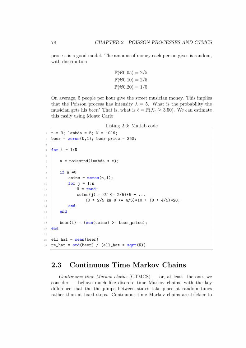
78 CHAPTER 2. POISSON PROCESSES AND CTMCS
process is a good model. The amount of money each person gives is random,with distribution
P(AC0.05) = 2/5
P(AC0.10) = 2/5
P(AC0.20) = 1/5.
On average, 5 people per hour give the street musician money. This impliesthat the Poisson process has intensity λ = 5. What is the probability themusician gets his beer? That is, what is ℓ = P(X3 ≥ 3.50). We can estimatethis easily using Monte Carlo.
Listing 2.6: Matlab code
1 t = 3; lambda = 5; N = 10^6;
2 beer = zeros(N,1); beer_price = 350;
3
4 for i = 1:N
5
6 n = poissrnd(lambda * t);
7
8 if n~=0
9 coins = zeros(n,1);
10 for j = 1:n
11 U = rand;
12 coins(j) = (U <= 2/5)*5 + ...
13 (U > 2/5 && U <= 4/5)*10 + (U > 4/5)*20;
14 end
15 end
16
17 beer(i) = (sum(coins) >= beer_price);
18 end
19
20 ell_hat = mean(beer)
21 re_hat = std(beer) / (ell_hat * sqrt(N))
2.3 Continuous Time Markov Chains
Continuous time Markov chains (CTMCS) — or, at least, the ones weconsider — behave much like discrete time Markov chains, with the keydifference that the the jumps between states take place at random timesrather than at fixed steps. Continuous time Markov chains are trickier to
2.3. CONTINUOUS TIME MARKOV CHAINS 79
work with than discrete time Markov chains, because there are a numberof technical issues and strange / pathological things that can happen. Thisbehavior is mainly related to situations where an infinite number of jumpscan happen in a finite time. In this course, we will not consider chains wheresuch things happen. This is because these chains can not really be simulatedand considering a smaller subset of continuous time Markov chains will besufficient for modeling most real world phenomena we might be interestedin.
The chains we consider can be described in two different but equivalentways: transition functions and infinitesimal genertors. Warning: these de-scriptions are not always equivalent or even valid when working with moregeneral classes of CTMCs.
2.3.1 Transition Function
Transition functions are the continuous time equivalent of the transitionmatrix, P , that we have already encountered when discussing discrete timeMarkov chains. That is, they are functions that allow us to calculate proba-bilities of the form Pi(Xt = j). More formally, a transition function is definedas follows.
Definition 2.3.1 (Transition function). A transition function pt(i, j) withi, j ∈ X and t ≥ 0 is a real-valued function satisfying the following properties
(i) pt(i, j) ≥ 0 for all i, j ∈ X and t ≥ 0.
(ii)∑
j∈X pt(i, j) = 1 for all i ∈ X and t ≥ 0.
(iii) limt↓0 pt(i, i) = p0(i, i) = 1 for all i ∈ X .
(iv) The Chapman-Kolmogorov equations:
ps+t(i, j) =∑
k∈X
ps(i, k)pt(k, j)
for all i, j ∈ X and t ≥ 0.
We can think of transitions functions as a family of matrices, P (t)t≥0,indexed by t. For a fixed value of t, (P (t))i,j = pt(i, j). We can write theproperties out again in terms of matrices:
Definition 2.3.2 (Transition function: Matrix Version). A transition func-tion is a family of matrices, P (t)t≥0 with the following properties.

80 CHAPTER 2. POISSON PROCESSES AND CTMCS
(i) They are non-negative, real-valued and∑
j∈X Pi,j = 1 for all i ∈ X andt ≥ 0. Matrices that are non-negative with unit row sums are calledstochastic matrices.
(ii) They satisfy the Chapman-Kolmogorov equations: P (s+t) = P (s)P (t).
2.3.2 Infinitesimal Generator
Definition 2.3.3. The infinitesimal generator (or Q-matrix) is a real valuedmatrix satisfying the following properties
(i) qi,j ≥ 0 for all i 6= j.
(ii)∑
j∈X qi,j = 0.
Thus, we require that qi,i = −∑j 6=i qi,j. Because it plays an importantrole in our treatment of CTMCs, we denote qi = −qi,i.
INF DEF. COMPETING POISSON PROCESS VERSION.EXAMPLE.
2.3.3 Continuous Time Markov Chains
FORMALLY. OUR VERSION.
2.3.4 The Jump Chain and Holding Times
If we only consider the sequence of states that a CTMC visits (by lookingat the value the CTMC takes immediately after each jump), we get a discretetime Markov chain Ynn≥0 called the jump chain of the CTMC. We call thetime spent in each state a holding time. Associate with a path of the jumpchain Y0, . . . , Yn is a sequence of holding times S1, . . . , Sn+1, where S1 is thetime spent in Y0 before jumping to Y1, S2 is the time spent in Y1 beforejumping to Y2, and so on. The definitions of the jump chain and holdingtimes are made clear in figure (REF).
PICTURE HERE
The jump chain Ynn≥0 is a discrete time Markov chain, so it can be de-scribed by a transition matrix J (we do not use P in order to avoid confusionwith the transition function P ). As it turns out, J can be written in termsof the Q-matrix.
2.3. CONTINUOUS TIME MARKOV CHAINS 81
Lemma 2.3.4. Given a CTMC with infinitesimal generator Q, the jumpmatrix J is defined by
Ji,i = 0
for all i ∈ X andJi,j =
qi,jqi
for all i, j ∈ X such that j 6= i.
The holding times are also defined by the Q-matrix.
Lemma 2.3.5. Given Y0, Y1, . . . , Yn, the holding times S1, . . . , Sn+1 are ex-ponential random variables with parameters qY0 , qY1 , . . . , qYn
.
Example 2.3.6. Consider the following CTMC.
PICTURE HERE
The Q matrix of this chain is given by
Q =
−λ λ 0µ −(λ+ µ) µ0 µ −µ
.
Thus, the transition matrix of the jump chain is
J =
0 1 0µ
λ+µ0 λ
λ+µ
0 1 0
,
and the amount of time spent in state 1 is Exp(λ), the amount of time spentin state 2 is Exp(λ+ µ) and the amount of time spent in state 3 is Exp(µ).
2.3.5 Examples of Continuous Time Markov Chains
Poisson Process
We are already quite familiar with one CTMC: the Poisson process. Thisprocess has exponential holding times (always with parameter λ) and a jumpchain that always increases by one. That is, the jump chain is of the form
J =
0 1 0 0 0 · · ·0 0 1 0 0 · · ·0 0 0 1 0 · · ·...
. . . . . . . . . . . . . . .
.

82 CHAPTER 2. POISSON PROCESSES AND CTMCS
This gives a Q-matrix of the form
Q =
−λ λ 0 0 0 · · ·0 −λ λ 0 0 · · ·0 0 −λ λ 0 · · ·...
. . . . . . . . . . . . . . .
.
Birth-Death Process
A Poisson process is sometimes called a pure birth process, as it models apopulation that is constantly growing. More generally, birth-death processesare simple models of populations where births and deaths happen at random.A simple example is the following
PICTURE HERE
The Q-matrix for this chain is of the form
Q =
−λ λ 0 0 0 · · ·µ −(µ+ λ) λ 0 0 · · ·0 µ −(µ+ λ) λ 0 · · ·...
. . . . . . . . . . . . . . .
.
2.3.6 Simulating Continuous Time Markov Chains
If we think about CTMCs in terms of jump chains and holding times,then the generic method for simulating them becomes obvious. We simplywait an exponential rate of time in each state, determined by the Q-matrix,the jump to the next state according to the J matrix. The jump chain itselfis simulated just as in the section on discrete time Markov chains. As withdiscrete time Markov chains, it is important to consider whether your chainis finite or infinite, as this usually changes the choice of how to encode J .If the chain is infinite, then it obviously is not possible to write out the Jmatrix.
Example 2.3.7 (A finite state space CTMC). Consider the following CTMC
PICTURE HERE,
with initial distribution λ = (1/2, 1/2, 0, 0). This chain has Q-matrix
Q =
−9 2 3 41 −4 3 01 2 −7 41 0 3 −4
.

2.3. CONTINUOUS TIME MARKOV CHAINS 83
and jump matrix
J =
0 2/9 3/9 4/91/4 0 3/4 01/7 2/7 0 4/71/4 0 3/4 0
.
The Matlab code for simulating this is as follows.
Listing 2.7: Matlab code
1 T = 10; t = 0;
2
3 Q = [-9 2 3 4; 1 -4 3 0; 1 2 -7 4; 1 0 3 -4];
4 J = [0 2/9 3/9 4/9; 1/4 0 3/4 0; 1/7 2/7 0 4/7; 1/4 0 3/4 0];
5
6 U = rand; X = (U <= 1/2) + 2*(U > 1/2);
7 jump_times = [0]; jump_chain = [X];
8
9 while t <= T
10 t = t + log(rand) / Q(X,X);
11 if t > T
12 break;
13 else
14 jump_times = [jump_times t];
15 X = min(find(rand<cumsum(J(X,:))));
16 jump_chain = [jump_chain X];
17 end
18 end
Example 2.3.8 (A birth-death process). Consider the birth-death processpictured in figure (REF) such that P(X0 = 0) = 1.
PICTURE HERE
We can implement this in Matlab by encoding the transition rule itself.
Listing 2.8: Matlab code
1 T = 100000; t = 0;
2 lambda = 2; mu = 0.25;
3
4 X = 0; jump_times = [0]; jump_chain = [X];
5
6 while t <= T
7 t = t - log(rand) / (lambda + X*mu);
8 if t > T

84 CHAPTER 2. POISSON PROCESSES AND CTMCS
9 break;
10 else
11 jump_times = [jump_times t];
12
13 if rand < lambda / (lambda + X*mu)
14 X = X + 1;
15 else
16 X = X - 1;
17 end
18 jump_chain = [jump_chain X];
19 end
20 end
2.3.7 The Relationship Between P and Q in the FiniteCase
In the finite case, we can write P directly in terms of Q. Remember thatP must satisfy P (s + t) = P (t)P (s). This implies that P should be somekind of exponential like function. In fact, we can write
P (t) = etQ
where etQ is the matrix exponential. It might at first be unclear how to definea matrix exponential. However, if we remember the Taylor series definitionof the exponential, then we realise we can write something equivalent usingmatrices. That is
P (t) =∞∑
k=0
(tQ)k
k!.
Warning! It is often very computationally challenging to compute a matrixexponential. The answer the computer gives you might not always be correct.In Matlab you need to use ‘expm’ rather than ‘exp’ if you wish to use thematrix exponential.
Example 2.3.9. Consider the CTMC given earlier with Q-matrix
Q =
−9 2 3 41 −4 3 01 2 −7 41 0 3 −4
and initial distribution λ = (1/2, 1/2, 0, 0). We can calculate

2.3. CONTINUOUS TIME MARKOV CHAINS 85
We can calculate etQ easily using Matlab. For t = 0.01, 0.1, 1, 10, 100 wehave
Listing 2.9: Matlab code
1 [1/2 1/2 0 0] * expm(.01 * Q) = 0.4619 0.4901 0.0285 0.0194
2 [1/2 1/2 0 0] * expm(.1 * Q) = 0.2472 0.4112 0.1896 0.1520
3 [1/2 1/2 0 0] * expm(1 * Q) = 0.1000 0.2061 0.3000 0.3939
4 [1/2 1/2 0 0] * expm(10 * Q) = 0.1000 0.2000 0.3000 0.4000
5 [1/2 1/2 0 0] * expm(100 * Q) = 0.1000 0.2000 0.3000 0.4000.
Looking at the example, we see that the distribution of the chain seemsto converge to a stationary distribution.
2.3.8 Irreducibility, Recurrence and Positive Recur-rence
As in the case of discrete time Markov chains, we want to establish con-ditions under which a CTMC has a unique stationary distribution. As ittranspires, these conditions are basically the same as those for discrete timeMarkov chains. This is because it is the structure of the jump chain thatdetermines whether a stationary distribution exists or not.
We say a state i leads to a state j (written i → j) if
Pi(Xt = j for some t ≥ 0) > 0.
We say i and j communicate (or i ↔ j) if i → j and j → i. The followingtheorem shows that it is sufficient to look at the jump chain in order todetermine communicating classes.
Theorem 2.3.10. Consider a CTMC Xtt≥0 with Q-matrix Q and jumpchain Ynn≥0. For distinct states i and j the following are equivalent
(i) i → j.
(ii) i → j for the jump chain.
(iii) qi,k1qk1,k2 · · · qkn,j > 0 for some n > 0 and states k1, . . . , kn.
(iv) pt(i, j) > 0 for all t > 0.
(v) pt(i, j) > 0 for some t > 0.
Proof. See [3].
86 CHAPTER 2. POISSON PROCESSES AND CTMCS
As in the discrete time case, a CTMC is irreducible if i ↔ j for alli, j ∈ X .
We say a state i is recurrent if
Pi(t ≥ 0 : Xt = i is unbounded) = 1.
We say a state j is transient if
Pi(t ≥ 0 : Xt = i is unbounded) = 0.
Again, it is sufficient to look at the jump chain to establish that theseproperties hold.
Theorem 2.3.11. Consider a CTMC Xtt≥0 with jump chain Ynn≥0.
(i) If i is recurrent for Ynn≥0 it is recurrent for Xtt≥0.
(ii) If i is transient for Ynn≥0 it is recurrent for Xtt≥0.
Proof. See [3].
A state i is positive recurrent if it is positive recurrent for the jump chain.
2.3.9 Invariant Measures and Stationary Distribution
Definition 2.3.12 (Invariant Measure). We say a measure (remember thisis a vector with non-negative elements) µ is invariant for a Q-matrix Q if
µQ = 0.
Invariant measures of CTMCs are closely related to invariant measuresfor the associated jump chain.
Theorem 2.3.13. Given a CTMC Xtt≥0 with Q-matrix Q and jump ma-trix J , the following are equivalent
(i) µ is invariant for Q.
(ii) νJ = ν, where νi = µiqi for all i ∈ X .
Note that 1/qi is the expected holding time in state i, so µ has elementsµi = νi/qi and is thus a invariant measure for the jump chain reweightedby the expected time spent in each state. Note that neither µ or ν is nec-essarily a probability distribution. Furthermore, even if µ is a probabilitydistribution, the ν defined in respect to it will probably not be a probability

2.3. CONTINUOUS TIME MARKOV CHAINS 87
distribution (until it is normalized). This is also the case if ν is a probabilitydistribution.
We are now able to give conditions for the existence of a unique stationarymeasure for a CTMC Xtt≥0. Unsurprisingly, these are the same conditionsas for discrete time Markov chains.
Theorem 2.3.14. Let Q be an irreducible Q matrix. Then, the followingare equivalent.
(i) Every state is positive recurrent.
(ii) Some state, i, is positive recurrent.
(iii) Q has an invariant distribution ρ.
Example 2.3.15. Given that a stationary distribution exists, we can findit by solving the linear system ρQ = 0. Consider the example from earlierwith Q matrix
Q =
−9 2 3 41 −4 3 01 2 −7 41 0 3 −4
.
Solving this system, we find ρ = (1/10, 2/10, 3/10, 4/10).
MENTION LIMITING DISTRIBUTION
2.3.10 Reversibility and Detailed Balance
As is the case with discrete time Markov chains, reversible chains areparticularly nice to work with. This largely due to detailed balance equationsholding.
Theorem 2.3.16. Given a CTMC Xtt≥0 with irreducible Q-matrix Qand invariant distribution ρ (which also serves as the initial distribution of
Xtt≥0). The process Xtt≥0 defined by Xt = XT−t is Markov (ρ, Q).
Additionally, Q is irreducible and has invariant distribution ρ.
Proof. See [3].
We say a CTMC is reversible if Q = Q.
Definition 2.3.17 (Detailed Balance Equations). A Q-matrix, Q, and ameasure µ are in detailed balance if
µiqi,j = µjqi,j for all i, j ∈ X .

88 CHAPTER 2. POISSON PROCESSES AND CTMCS
The following theorem is more or less identical to the discrete version.
Theorem 2.3.18. If a Q-matrix, Q, and a measure µ are in detailed balancethen µ is invariant for Q.
Proof. For a given i ∈ X , we have
(µQ)i =∑
j∈X
µjqj,i =∑
j∈X
µiqi,j = 0.
The only CTMCs that satisfy detailed balance are reversible ones.
Theorem 2.3.19. Let Q be an irreducible Q-matrix and ρ a distribution.Suppose Xtt≥0 is Markov (ρ, Q). Then, the following are equivalent
(i) Xtt≥0 is reversible.
(ii) Q and ρ are in detailed balance.
Proof. See [3].

Chapter 3
Gaussian Processes andStochastic DifferentialEquations
3.1 Gaussian Processes
Gaussian processes are a reasonably large class of processes that havemany applications, including in finance, time-series analysis and machinelearning. Certain classes of Gaussian processes can also be thought of asspatial processes. We will use these as a vehicle to start considering moregeneral spatial objects.
Definition 3.1.1 (Gaussian Process). A stochastic process Xtt≥0 is Gaus-sian if, for any choice of times t1, . . . , tn, the random vector (Xt1 , . . . , Xtn)has a multivariate normal distribution.
3.1.1 The Multivariate Normal Distribution
Because Gaussian processes are defined in terms of the multivariate nor-mal distribution, we will need to have a pretty good understanding of thisdistribution and its properties.
Definition 3.1.2 (Multivariate Normal Distribution). A vectorX = (X1, . . . , Xn)is said to be multivariate normal (multivariate Gaussian) if all linear combi-nations of X, i.e. all random variables of the form
n∑
k=1
αkXk
have univariate normal distributions.
89

90 CHAPTER 3. GAUSSIAN PROCESSES ETC.
This is quite a strong definition. Importantly, it implies that, even if all ofits components are normally distributed, a random vector is not necessarilymultivariate normal.
Example 3.1.3 (A random vector with normal marginals that is not multi-variate normal). Let X1 ∼ N(0, 1) and
X2 =
X1 if |X1| ≤ 1
−X1 if |X1| > 1.
Note that X2 ∼ N(0, 1). However, X1 + X2 is not normally distributed,because |X1+X2| ≤ 2, which implies X1+X2 is bounded and, hence, cannotbe normally distributed.
Linear transformations of multivariate normal random vectors are, again,multivariate normal.
Lemma 3.1.4. Suppose X = (X1, . . . , Xn) is multivariate normal and A isan m× n real-valued matrix. Then, Y = AX is also multivariate normal.
Proof. Any linear combination of Y1, . . . , Ym is a linear combination of linearcombinations of X1, . . . , Xn and, thus, univariate normal.
Theorem 3.1.5. A multivariate normal random vector X = (X1, . . . , Xn)is completely described by a mean vector µ = EX and a covariance matrixΣ = Var(X).
Proof. The distribution of X is described by its characteristic function whichis
Eexp iθ⊺X = Eexp
i
n∑
i=1
θiXi
.
Now, we know∑n
i=1 θiXi is a univariate normal random variable (becauseX is multivariate normal). Let m = E
∑ni=1 θiXi and σ2 = Var (
∑ni=1 θiXi).
Then,
E
i
n∑
i=1
θiXi
= exp
im− 1
2σ2
.
Now
m = E
n∑
i=1
θiXi =n∑
i=1
θiµi
and
σ2 = Var
(n∑
i=1
θiXi
)=
n∑
i=1
n∑
j=1
θiθjCov(Xi, Xj) =n∑
j=1
n∑
j=1
θiθjΣi,j .
So, everything is specified by µ and Σ.

3.1. GAUSSIAN PROCESSES 91
INDEPENDENCE
There is nothing too difficult about dealing with the mean vector µ. How-ever, the covariance matrix makes things pretty difficult, especially when wewish to simulate a high dimensional random vector. In order to simulateGaussian processes effectively, we need to exploit as many properties of co-variance matrices as possible.
Symmetric Positive Definite and Semi-Positive Definite Matrices
Covariance matrices are members of a family of matrices called symmetric
positive definite matrices.
Definition 3.1.6 (Positive Definite Matrices (Real-Valued)). An n×n real-valued matrix, A, is positive definite if and only if
x⊺Ax > 0 for all x 6= 0.
If A is also symmetric, then A is called symmetric positive definite (SPD).Some important properties of SPD matrices are
(i) rank(A) = n.
(ii) |A| > 0.
(iii) Ai,i > 0.
(iv) A−1 is SPD.
Lemma 3.1.7 (Necessary and sufficient conditions for an SPD). The fol-lowing are necessary and sufficient conditions for an n × n matrix A to beSPD
(i) All the eigenvalues λ1, . . . , λn of A are strictly positive.
(ii) There exists a unique matrix C such that A = CC⊺, where C is a real-valued lower-triangular matrix with positive diagonal entries. This iscalled the Cholesky decomposition of A.
Definition 3.1.8 (Positive Semi-definite Matrices (Real-Valued)). An n×nreal-valued matrix, A, is positive semi-definite if and only if
x⊺Ax ≥ 0 for all x 6= 0.
92 CHAPTER 3. GAUSSIAN PROCESSES ETC.
If A is also symmetric, then A is called symmetric positive semi-definite(SPSD). Note that if A is an SPSD then there is a real-valued decomposition
A = LL⊺,
though it is not necessarily unique and L may have zeroes on the diagonals.
Lemma 3.1.9. Covariance matrices are SPSD.
Proof. Given an n × 1 real-valued vector x and a random vector Y withcovariance matrix Σ, we have
Var (x⊺Y) = x⊺Var (Y)x.
Now this must be non-negative (as it is a variance). That is, it must be thecase that
x⊺Var (Y)x ≥ 0,
so Σ is positive semi-definite. Symmetry comes from the fact that Cov(X, Y ) =Cov(Y,X).
Lemma 3.1.10. SPSD matrices are covariance matrices.
Proof. Let A be an SPSD matrix and Z be a vector of random variables withVar(Z) = I. Now, as A is SPSD, A = LL⊺. So,
Var(LZ) = LVar(Z)L⊺ = LIL⊺ = A,
so A is the covariance matrix of LZ.
COVARIANCE POS DEF ...
Densities of Multivariate Normals
If X = (X1, . . . , Xn) is N(µ,Σ) and Σ is positive definite, then X has thedensity
f(x) = f(x1, . . . , xn) =1√
(2π)n|Σ|exp
−1
2(x− µ)⊺Σ−1(x− µ)
.
3.1. GAUSSIAN PROCESSES 93
Simulating Multivariate Normals
One possible way to simulate a multivariate normal random vector isusing the Cholesky decomposition.
Lemma 3.1.11. If Z ∼ N(0, I), Σ = AA⊺ is a covariance matrix, andX = µ+ AZ, then X ∼ N(µ,Σ).
Proof. We know from lemma 3.1.4 that AZ is multivariate normal and sois µ + AZ. Because a multivariate normal random vector is completelydescribed by its mean vector and covariance matrix, we simple need to findEX and Var(X). Now,
EX = Eµ+ EAZ = µ+ A0 = µ
and
Var(X) = Var(µ+ AZ) = Var(AZ) = AVar(Z)A⊺ = AIA⊺ = AA⊺ = Σ.
Thus, we can simulate a random vector X ∼ N(µ,Σ) by
(i) Finding A such that Σ = AA⊺.
(ii) Generating Z ∼ N(0, I).
(iii) Returning X = µ+ AZ.
Matlab makes things a bit confusing because its function ‘chol’ producesa decomposition of the form B⊺B. That is, A = B⊺. It is important tobe careful and think about whether you want to generate a row or columnvector when generating multivariate normals.
The following code produces column vectors.
Listing 3.1: Matlab code
1 mu = [1 2 3]’;
2 Sigma = [3 1 2; 1 2 1; 2 1 5];
3 A = chol(Sigma);
4 X = mu + A’ * randn(3,1);
The following code produces row vectors.
Listing 3.2: Matlab code
1 mu = [1 2 3];
2 Sigma = [3 1 2; 1 2 1; 2 1 5];
3 A = chol(Sigma);
4 X = mu + randn(1,3) * A;
94 CHAPTER 3. GAUSSIAN PROCESSES ETC.
The complexity of the Cholesky decomposition of an arbitrary real-valuedmatrix is O(n3) floating point operations.
3.1.2 Simulating a Gaussian Processes Version 1
Because Gaussian processes are defined to be processes where, for anychoice of times t1, . . . , tn, the random vector (Xt1 , . . . , Xtn) has a multivariatenormal density and a multivariate normal density is completely describe bya mean vector µ and a covariance matrix Σ, the probability distribution ofGaussian process is completely described if we have a way to construct themean vector and covariance matrix for an arbitrary choice of t1, . . . , tn.
We can do this using an expectation function
µ(t) = EXt
and a covariance function
r(s, t) = Cov(Xs, Xt).
Using these, we can simulate the values of a Gaussian process at fixed timest1, . . . , tn by calculating µ where µi = µ(t1) and Σ, where Σi,j = r(ti, tj) andthen simulating a multivariate normal vector.
In the following examples, we simulate the Gaussian processes at evenlyspaced times t1 = 1/h, t2 = 2/h, . . . , tn = 1.
Example 3.1.12 (Brownian Motion). Brownian motion is a very importantstochastic process which is, in some sense, the continuous time continuousstate space analogue of a simple random walk. It has an expectation functionµ(t) = 0 and a covariance function r(s, t) = min(s, t).
Listing 3.3: Matlab code
1 %use mesh size h
2 m = 1000; h = 1/m; t = h : h : 1;
3 n = length(t);
4
5 %Make the mean vector
6 mu = zeros(1,n);
7 for i = 1:n
8 mu(i) = 0;
9 end
10
11 %Make the covariance matrix
12 Sigma = zeros(n,n);
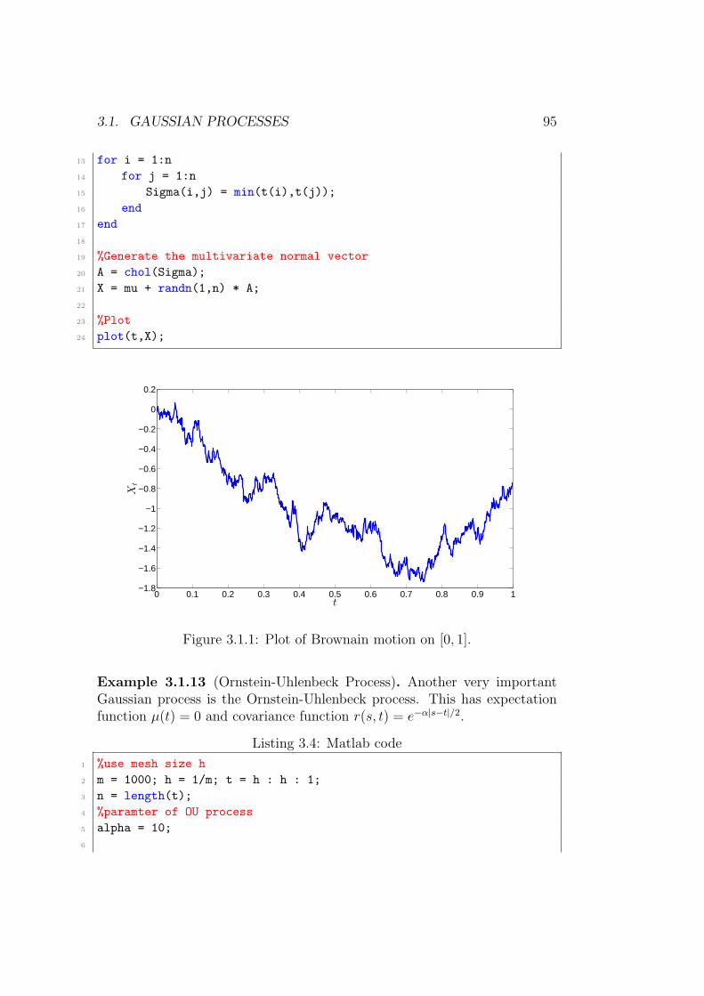
3.1. GAUSSIAN PROCESSES 95
13 for i = 1:n
14 for j = 1:n
15 Sigma(i,j) = min(t(i),t(j));
16 end
17 end
18
19 %Generate the multivariate normal vector
20 A = chol(Sigma);
21 X = mu + randn(1,n) * A;
22
23 %Plot
24 plot(t,X);
0 0.1 0.2 0.3 0.4 0.5 0.6 0.7 0.8 0.9 1−1.8
−1.6
−1.4
−1.2
−1
−0.8
−0.6
−0.4
−0.2
0
0.2
t
Xt
Figure 3.1.1: Plot of Brownain motion on [0, 1].
Example 3.1.13 (Ornstein-Uhlenbeck Process). Another very importantGaussian process is the Ornstein-Uhlenbeck process. This has expectationfunction µ(t) = 0 and covariance function r(s, t) = e−α|s−t|/2.
Listing 3.4: Matlab code
1 %use mesh size h
2 m = 1000; h = 1/m; t = h : h : 1;
3 n = length(t);
4 %paramter of OU process
5 alpha = 10;
6

96 CHAPTER 3. GAUSSIAN PROCESSES ETC.
7 %Make the mean vector
8 mu = zeros(1,n);
9 for i = 1:n
10 mu(i) = 0;
11 end
12
13 %Make the covariance matrix
14 Sigma = zeros(n,n);
15 for i = 1:n
16 for j = 1:n
17 Sigma(i,j) = exp(-alpha * abs(t(i) - t(j)) / 2);
18 end
19 end
20
21 %Generate the multivariate normal vector
22 A = chol(Sigma);
23 X = mu + randn(1,n) * A;
24
25 %Plot
26 plot(t,X);
0 0.1 0.2 0.3 0.4 0.5 0.6 0.7 0.8 0.9 1−1.5
−1
−0.5
0
0.5
1
1.5
2
2.5
3
t
Xt
Figure 3.1.2: Plot of an Ornstein-Uhlenbeck process on [0, 1] with α = 10.
Example 3.1.14 (Fractional Brownian Motion). Fractional Brownian mo-tion (fBm) is a generalisation of Brownian Motion. It has expectation func-tion µ(t) = 0 and covariance function Cov(s, t) = 1/2(t2H + s2H − |t− s|2H),
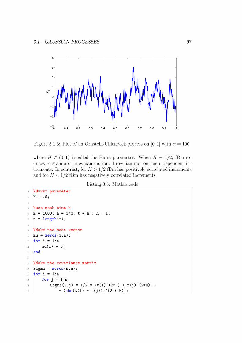
3.1. GAUSSIAN PROCESSES 97
0 0.1 0.2 0.3 0.4 0.5 0.6 0.7 0.8 0.9 1−3
−2
−1
0
1
2
3
4
t
Xt
Figure 3.1.3: Plot of an Ornstein-Uhlenbeck process on [0, 1] with α = 100.
where H ∈ (0, 1) is called the Hurst parameter. When H = 1/2, fBm re-duces to standard Brownian motion. Brownian motion has independent in-crements. In contrast, for H > 1/2 fBm has positively correlated incrementsand for H < 1/2 fBm has negatively correlated increments.
Listing 3.5: Matlab code
1 %Hurst parameter
2 H = .9;
3
4 %use mesh size h
5 m = 1000; h = 1/m; t = h : h : 1;
6 n = length(t);
7
8 %Make the mean vector
9 mu = zeros(1,n);
10 for i = 1:n
11 mu(i) = 0;
12 end
13
14 %Make the covariance matrix
15 Sigma = zeros(n,n);
16 for i = 1:n
17 for j = 1:n
18 Sigma(i,j) = 1/2 * (t(i)^(2*H) + t(j)^(2*H)...
19 - (abs(t(i) - t(j)))^(2 * H));

98 CHAPTER 3. GAUSSIAN PROCESSES ETC.
20 end
21 end
22
23 %Generate the multivariate normal vector
24 A = chol(Sigma);
25 X = mu + randn(1,n) * A;
26
27 %Plot
28 plot(t,X);
0 0.1 0.2 0.3 0.4 0.5 0.6 0.7 0.8 0.9 1−2
−1.5
−1
−0.5
0
0.5
1
1.5
2
t
Xt
Figure 3.1.4: Plot of fractional Brownian motion on [0, 1] with H = 0.1.
3.1.3 Stationary and Weak Stationary Gaussian Pro-cesses
Gaussian processes (and stochastic processes in general) are easier to workwith if they are stationary stochastic processes.
Definition 3.1.15 (Stationary Stochastic Process). A stochastic processXtt≥0 is said to be stationary if the random vectors (Xt1 , Xt2 , . . . , Xtn)and (Xt1+s, Xt2+s, . . . , Xtn+s) have the same distribution for all choices ofs, n and t1, t2, . . . , tn.
An example of such a process would be an irreducible positive recurrentcontinuous time Markov chain started from its stationary distribution.
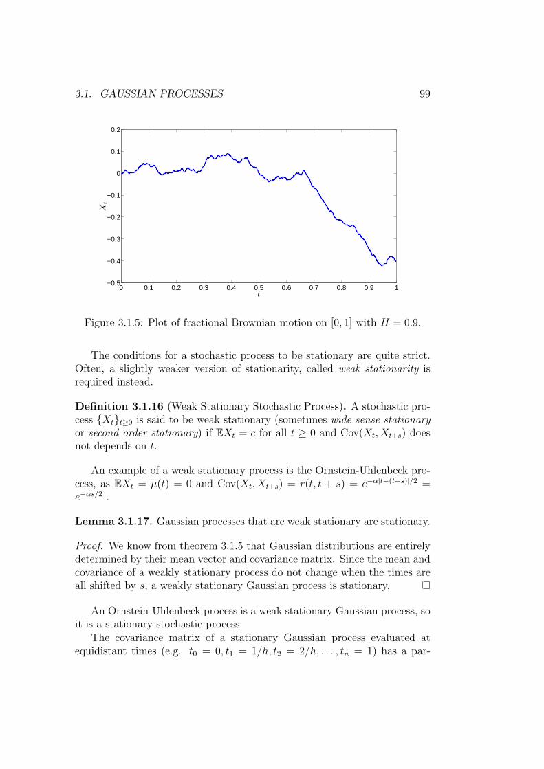
3.1. GAUSSIAN PROCESSES 99
0 0.1 0.2 0.3 0.4 0.5 0.6 0.7 0.8 0.9 1−0.5
−0.4
−0.3
−0.2
−0.1
0
0.1
0.2
t
Xt
Figure 3.1.5: Plot of fractional Brownian motion on [0, 1] with H = 0.9.
The conditions for a stochastic process to be stationary are quite strict.Often, a slightly weaker version of stationarity, called weak stationarity isrequired instead.
Definition 3.1.16 (Weak Stationary Stochastic Process). A stochastic pro-cess Xtt≥0 is said to be weak stationary (sometimes wide sense stationary
or second order stationary) if EXt = c for all t ≥ 0 and Cov(Xt, Xt+s) doesnot depends on t.
An example of a weak stationary process is the Ornstein-Uhlenbeck pro-cess, as EXt = µ(t) = 0 and Cov(Xt, Xt+s) = r(t, t + s) = e−α|t−(t+s)|/2 =e−αs/2 .
Lemma 3.1.17. Gaussian processes that are weak stationary are stationary.
Proof. We know from theorem 3.1.5 that Gaussian distributions are entirelydetermined by their mean vector and covariance matrix. Since the mean andcovariance of a weakly stationary process do not change when the times areall shifted by s, a weakly stationary Gaussian process is stationary.
An Ornstein-Uhlenbeck process is a weak stationary Gaussian process, soit is a stationary stochastic process.
The covariance matrix of a stationary Gaussian process evaluated atequidistant times (e.g. t0 = 0, t1 = 1/h, t2 = 2/h, . . . , tn = 1) has a par-

100 CHAPTER 3. GAUSSIAN PROCESSES ETC.
ticularly nice form:
Σ =
σ0 σ1 σ2 · · · σn
σ1 σ0 σ1 · · · σn−1
σ2 σ1 σ0. . . σn−2
......
.... . .
...σn σn−1 σn−2 · · · σ0
.
Technically, it is a symmetric Toeplitz matrix.
Definition 3.1.18 (Toeplitz Matrix). A Toeplitz matrix, A, is a matrixwhere each diagonal takes a single, constant value. That is, ai,j = ai+1,j+1
for all i, j ∈ 1, . . . , n− 1.
We can embed this matrix in a 2n× 2n circulant matrix
Σ =
σ0 σ1 σ2 · · · σn σn−1 σn−2 · · · σ2 σ1
σ1 σ0 σ1 · · · σn−1 σn σn−1 · · · σ3 σ2
σ2 σ1 σ0. . . σn−2 σn−1 σn · · · σ4 σ3
.... . . . . . . . . . . . . . . . . . . . . . . .
...σn σn−1 σn−2 · · · σ0 σ1 σ2 · · · σn σn−1
σn−1 σn σn−1 · · · σ1 σ0 σ1 · · · σn−3 σn−2
σn−2 σn−1 σn · · · σ2 σ1 σ0 · · · σn−4 σn−3
σn−3 σn−2 σn−1 · · · σ3 σ2 σ1 · · · σn−5 σn−4...
. . . . . . . . . . . . . . . . . . . . . . . ....
σ1 σ2 σ3 · · · σn−1 σn−2 σn−3 · · · σ1 σ0
.
If σ0 ≥ σ1 ≥ · · · ≥ σn ≥ 0 and 2σk ≤ σk−1 + σk+1 for k = 1, . . . , n − 1,then C is also a covariance matrix.
Definition 3.1.19 (Circulant Matrix). A circulant matrix is a matrix of theform
B =
b0 bn−1 · · · b2 b1b1 b0 · · · b3 b2...
. . . . . . . . ....
bn−1 bn−2 · · · b1 b0
.
It is fully specified by b, its first column. The last row of a circulant matrix isthe first column in reverse order. The remaining rows are cyclic permutationsof this row.

3.1. GAUSSIAN PROCESSES 101
This might not seem very useful, but the strength of this representationcomes from its link to the discrete Fourier transform and, through it, to thatwonder of numerical analysis: the Fast Fourier Transform (FFT).
Definition 3.1.20 (Discrete Fourier Transform). Given a complex valuedvector x = (x0, . . . , xn)
⊺, we define its discrete Fourier transform by x =(x0, . . . , xn−1)
⊺, where
xj =n−1∑
k=0
e−(2πi/n)jkxk =n−1∑
k=0
ωjkxk
for j = 0, . . . , n− 1, where ω = e−(2πi/n).
Note that the discrete Fourier transform is equivalent to calculating
x = Fx,
where
F =
1 1 1 · · · 11 ω ω2 · · · ωn−1
1 ω2 ω4 . . . ω2(n−1)
......
.... . .
...
1 ωn−1 ω2(n−1) · · · ω(n−1)2
.
As it turns out, F−1 = F /n. Normally solving the system x = Fx wouldrequire O(n2) steps, but the FFT reduces this to O(n log n) steps.
The link to circulant matrices is as follows. Let b = (b0, b1, . . . , bn−1)⊺ be
a complex-valued vector. The circulant matrix corresponding to b is
B =
b0 bn−1 · · · b2 b1b1 b0 · · · b3 b2...
. . . . . . . . ....
bn−1 bn−2 · · · b1 b0
.
The eigenvalues of B, λ0, . . . , λn−1 are given by
λj = b⊺fj,
for j = 0, . . . , n− 1, with associated eigenvectors f0, . . . , fn−1, where fj is thejth column of F .
If B is diagonalizable, then it can be written as B = PDP−1, where thecolumns of P are the right eigenvectors of B and D = diag(λ0, . . . , λn−1).Thus, if we can calculate
λ = (λ0, . . . , λn−1) = Fb

102 CHAPTER 3. GAUSSIAN PROCESSES ETC.
and
E = F√diag(λ/n),
then
EE⊺ = Fdiag(λ)F /n = Fdiag(λ)F−1 = B.
In other words E is the complex square-root of the matrix B.Let B be the covariance matrix of a zero-mean Gaussian process evaluated
at equidistant steps. Now, if we write E = E1 + iE2 then
B = EE⊺ = (E1 + iE2) (E⊺
1 − iE⊺
2 ) = E1E⊺
1 + E2E⊺
2 + i (E2E⊺
1 − E1E⊺
2 )
As B is real-valued, B = E1E⊺
1 + E2E⊺
2 .Let Z1 and Z2 be N(0, I) and define
X = EZ = (E1 + iE2)(Z1 + iZ2) = (E1Z1 − E2Z2) + i(E2Z1 + E1Z2).
Let
X1 = R(X) = E1Z1 − E2Z2
and
X2 = I(X) = E2Z1 + E1Z2.
Then, clearly, EX1 = 0 and
Var(X1) = Var(E1Z1 − E2Z2) = E1E⊺
1 + E2E⊺
2 = B.
The calculation for X2 is more or less identical. Note X1 and X2 are notindependent of one another.
This gives the following algorithm for generating a stationary Gaussianprocess at equidistant intervals. Using the FFT, the algorithm is O(n log n).
Algorithm 3.1.1 (Generating a Stationary Gaussian Process).
(i) Set c = (σ0, σ1, . . . , σn−1, σn, σn−1, . . . , σ1).
(ii) Compute λ = Fc using the FFT.
(iii) Generate Z = Y1 +Y2 where Y1,Y2 ∼ N(0, I).
(iv) Compute η =√diag(λ/n)Z.
(v) Compute V = Fη and let A be the first n+ 1 elements of V.
(vi) Output X = R(A).
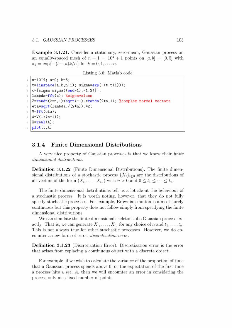
3.1. GAUSSIAN PROCESSES 103
Example 3.1.21. Consider a stationary, zero-mean, Gaussian process onan equally-spaced mesh of n + 1 = 104 + 1 points on [a, b] = [0, 5] withσk = exp−(b− a)k/n for k = 0, 1, . . . , n.
Listing 3.6: Matlab code
1 n=10^4; a=0; b=5;
2 t=linspace(a,b,n+1); sigma=exp(-(t-t(1)));
3 c=[sigma sigma((end-1):-1:2)]’;
4 lambda=fft(c); %eigenvalues
5 Z=randn(2*n,1)+sqrt(-1).*randn(2*n,1); %complex normal vectors
6 eta=sqrt(lambda./(2*n)).*Z;
7 V=fft(eta);
8 A=V(1:(n+1));
9 X=real(A);
10 plot(t,X)
3.1.4 Finite Dimensional Distributions
A very nice property of Gaussian processes is that we know their finite
dimensional distributions.
Definition 3.1.22 (Finite Dimensional Distributions). The finite dimen-sional distributions of a stochastic process Xtt≥0 are the distributions ofall vectors of the form (Xt1 , . . . , Xtn) with n > 0 and 0 ≤ t1 ≤ · · · ≤ tn.
The finite dimensional distributions tell us a lot about the behaviour ofa stochastic process. It is worth noting, however, that they do not fullyspecify stochastic processes. For example, Brownian motion is almost surelycontinuous but this property does not follow simply from specifying the finitedimensional distributions.
We can simulate the finite dimensional skeletons of a Gaussian process ex-actly. That is, we can generate Xt1 , . . . , Xtn for any choice of n and t1, . . . , tn.This is not always true for other stochastic processes. However, we do en-counter a new form of error, discretization error.
Definition 3.1.23 (Discretization Error). Discretization error is the errorthat arises from replacing a continuous object with a discrete object.
For example, if we wish to calculate the variance of the proportion of timethat a Gaussian process spends above 0, or the expectation of the first timea process hits a set, A, then we will encounter an error in considering theprocess only at a fixed number of points.

104 CHAPTER 3. GAUSSIAN PROCESSES ETC.
Discretization error needs to be considered when we decide on a sam-pling budget. Consider, for example, an evenly spaced mesh of points t1 =1/m, t2 = 2/m, . . . tn = 1. As m gets bigger, the mesh gets finer and thediscretization error gets smaller. We still have statistical error, however, sowe need to make sure we generate a large enough sample of realizations ofthe stochastic process (determined by the sample size N). The total workdone by our simulation is then given by
work = number of samples× work to make one sample = Nf(m).
Usually, f grows at least linearly in m. In the case of Cholesky decompo-sition, for example, it is O(m3). For a fixed level of work, we need to decideon how much effort to allocate to reducing discretization error (how large mshould be) and how much effort to allocate to reducing statistical error (howlarge N should be). Finding the optimal tradeoff can be difficult. We willconsider such tradeoffs in a number of situations.
3.1.5 Marginal and Conditional Multivariate NormalDistributions
The multivariate normal distribution has many attractive properties. Inparticular, its marginal distributions are also multivariate normal. In addi-tion, if we condition on part of the a multivariate normal vector, the remain-ing values are also multivariate normal.
To see this, we need to write normal random vectors in the appropriateform. LetX ∼ N(µ,Σ). We can decomposeX into two parts,X = (X1,X2)
⊺.We can then write µ as (µ1,µ2)
⊺ and Σ as
Σ =
[Σ11 Σ12
Σ21 Σ22
].
Theorem 3.1.24 (Multivariate Normal Marginal Distributions). GivenX =(X1,X2) ∼ N(µ,Σ),
X1 ∼ N(µ1,Σ11),
andX2 ∼ N(µ2,Σ22).
Theorem 3.1.25 (Multivariate Normal Conditional Distributions). GivenX = (X1,X2) ∼ N(µ,Σ), X2 conditional on X1 is multivariate normal with
E[X2 |X1] = µ2 + Σ21Σ−111 (X1 − µ1)
andVar(X2 |X1) = Σ22 − Σ21Σ
−111 Σ12.
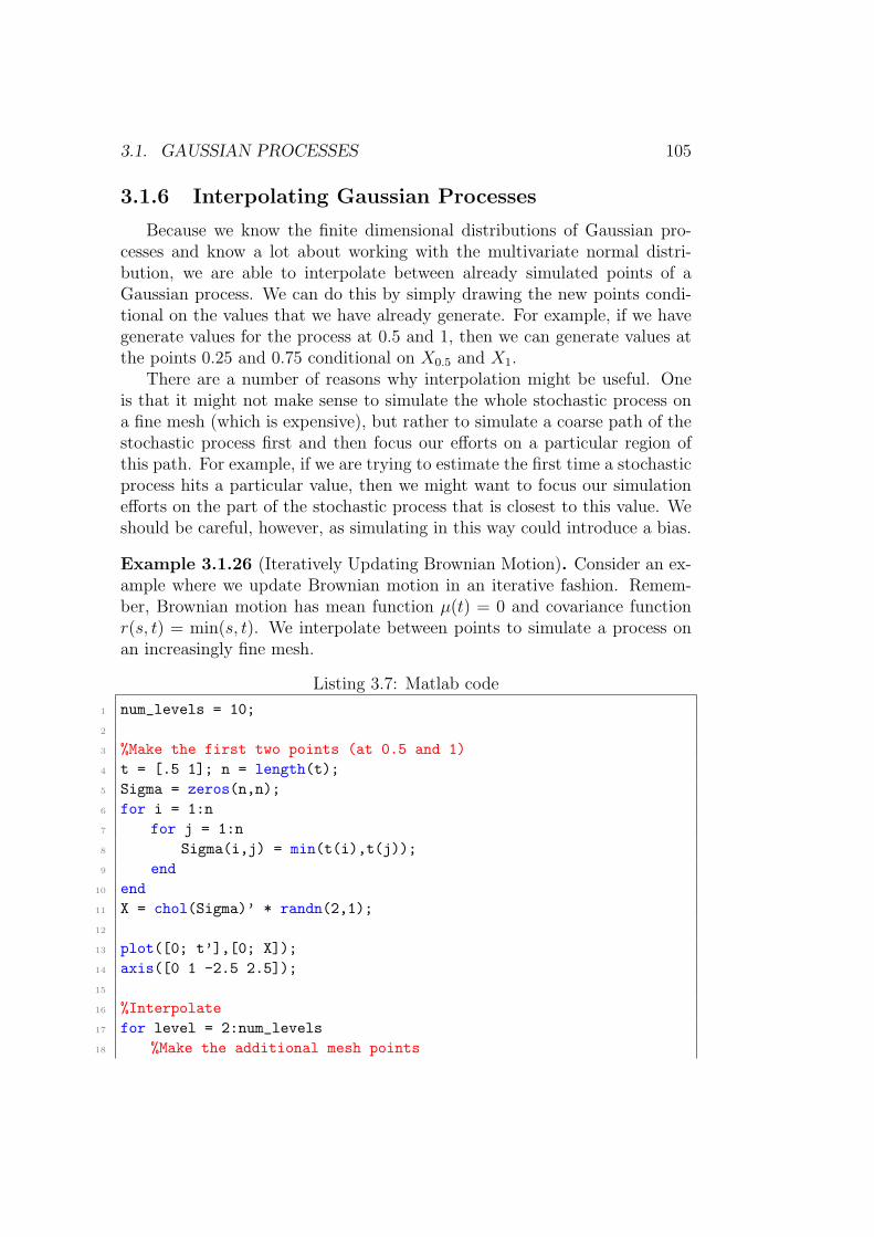
3.1. GAUSSIAN PROCESSES 105
3.1.6 Interpolating Gaussian Processes
Because we know the finite dimensional distributions of Gaussian pro-cesses and know a lot about working with the multivariate normal distri-bution, we are able to interpolate between already simulated points of aGaussian process. We can do this by simply drawing the new points condi-tional on the values that we have already generate. For example, if we havegenerate values for the process at 0.5 and 1, then we can generate values atthe points 0.25 and 0.75 conditional on X0.5 and X1.
There are a number of reasons why interpolation might be useful. Oneis that it might not make sense to simulate the whole stochastic process ona fine mesh (which is expensive), but rather to simulate a coarse path of thestochastic process first and then focus our efforts on a particular region ofthis path. For example, if we are trying to estimate the first time a stochasticprocess hits a particular value, then we might want to focus our simulationefforts on the part of the stochastic process that is closest to this value. Weshould be careful, however, as simulating in this way could introduce a bias.
Example 3.1.26 (Iteratively Updating Brownian Motion). Consider an ex-ample where we update Brownian motion in an iterative fashion. Remem-ber, Brownian motion has mean function µ(t) = 0 and covariance functionr(s, t) = min(s, t). We interpolate between points to simulate a process onan increasingly fine mesh.
Listing 3.7: Matlab code
1 num_levels = 10;
2
3 %Make the first two points (at 0.5 and 1)
4 t = [.5 1]; n = length(t);
5 Sigma = zeros(n,n);
6 for i = 1:n
7 for j = 1:n
8 Sigma(i,j) = min(t(i),t(j));
9 end
10 end
11 X = chol(Sigma)’ * randn(2,1);
12
13 plot([0; t’],[0; X]);
14 axis([0 1 -2.5 2.5]);
15
16 %Interpolate
17 for level = 2:num_levels
18 %Make the additional mesh points

106 CHAPTER 3. GAUSSIAN PROCESSES ETC.
19 t_new = 1/2^level : 2/2^level : (2^level-1)/(2^level);
20 n_new = length(t_new);
21
22 %Record the time points for the whole process
23 t_temp = [t t_new];
24 n_temp = length(t_temp);
25
26 %Make a covariance matrix for the whole thing
27 Sigma_temp = zeros(n_temp,n_temp);
28 for i = 1:n_temp
29 for j = 1:n_temp
30 Sigma_temp(i,j) = min(t_temp(i),t_temp(j));
31 end
32 end
33
34 %Make the separate Sigma components
35 Sigma_11 = Sigma;
36 Sigma_21 = Sigma_temp(n+1:n_temp, 1:n);
37 Sigma_12 = Sigma_temp(1:n, n+1:n_temp);
38 Sigma_22 = Sigma_temp(n+1:n_temp, n+1:n_temp);
39
40 temp_mean = Sigma_21 * inv(Sigma_11) * X;
41 Sigma_new = Sigma_22 - Sigma_21 * inv(Sigma_11) * Sigma_12;
42 X_new = temp_mean + chol(Sigma_new)’ * randn(n_new,1);
43 X = [X; X_new];
44 t = t_temp;
45 n = n_temp;
46 Sigma = Sigma_temp;
47 [dummy index] = sort(t);
48 another_dummy = waitforbuttonpress;
49
50 plot([0; t(index)’],[0; X(index)]);
51 axis([0 1 -2.5 2.5]);
52 end
3.1.7 Markovian Gaussian Processes
If a Gaussian process, Xtt≥0, is Markovian, we can exploit this structureto simulate the process much more efficiently. Because Xtt≥0 is Markovian,we can use we only need to know the value of Xti in order to generate Xti+1
.Define
σi,i+1 = Cov(Xti , Xti+1)

3.1. GAUSSIAN PROCESSES 107
andµi = EXti .
By theorem 3.1.24, we know that (Xti , Xti+1)⊺ has a multivariate normal
distribution. In particular,(
Xti
Xti+1
)∼ N
((µi
µi+1
),
(σi,i σi,i+1
σi,i+1 σi+1,i+1
)).
Using theorem 3.1.25, we have
Xti+1|Xti = xi ∼ N
(µi +
σi,i+1
σi, i(xi − µi) , σi+1,i+1 −
σ2i,i+1
σi,i
).
Algorithm 3.1.2 (Generating a Markovian Gaussian Process).
(i) Draw Z ∼ N(0, 1). Set Xt1 = µ1 +√σi,iZ.
(ii) For i = 1, . . . ,m− 1 draw Z ∼ N(0, 1) and set
Xti+1= µi +
σi,i+1
σi, i(Xti − µi) +
√σi+1,i+1 −
σ2i,i+1
σi,i
Z.
Example 3.1.27 (Brownian Motion). Consider Brownian motion, which isa Markov process. Now,
µi = EXti = 0
andσi,i+1 = min(ti, ti+1) = ti.
So, our updating formula is
Xti+1= Xti +
(√ti+1 − ti
)Z.
Listing 3.8: Matlab code
1 m = 10^4; X = zeros(m,1);
2 h = 1/m;
3 X(1) = sqrt(h)*randn;
4
5 for i = 1:m-1
6 X(i+1) = X(i) + sqrt(h) * randn;
7 end
8
9 plot(h:h:1,X);

108 CHAPTER 3. GAUSSIAN PROCESSES ETC.
Example 3.1.28 (Ornstein-Uhlenbeck Process). The Ornstein-Uhlenbeckprocess has
µi = EXti = 0
with
σi,i+1 = expα|ti − ti+1|/2and σi,i = 1. So, our updating formula is
Xti+1= exp−α|ti − ti+1|/2Xti +
(√1− expα|ti − ti+1|
)Z.
Listing 3.9: Matlab code
1 alpha = 50; m = 10^4;
2
3 X = zeros(m,1); h = 1/m;
4 X(1) = randn;
5
6 for i = 1:m-1
7 X(i+1) = exp(-alpha * h / 2)*X(i)...
8 + sqrt(1 - exp(-alpha * h))*randn;
9 end
10
11 plot(h:h:1,X);
3.2 Brownian Motion
One of the most fundamental stochastic processes. It is a Gaussian pro-cess, a Markov process, a Levy process, a Martingale and a process that isclosely linked to the study of harmonic functions (do not worry if you do notknow all these terms). It can be used as a building block when consideringmany more complicated processes. For this reason, we will consider it inmuch more depth than any other Gaussian process.
Definition 3.2.1 (Brownian Motion). A stochastic process Wtt≥0 is calledBrownian motion (a Wiener process) if:
(i) It has independent increments.
(ii) It has stationary increments.
(iii) Wt ∼ N(0, t) for all t ≥ 0.

3.2. BROWNIAN MOTION 109
(iv) It has almost surely continuous sample paths. That is,
P(ω : X(t, ω) is continuous in t) = 1.
This definition implies that the increments of Brownian motion are nor-mally distributed. Specifically, Wt+s−Wt ∼ N(0, s). This implies the follow-ing simualtion scheme.
Listing 3.10: Matlab code
1 m = 10^3; h = 1/m;
2 X = cumsum(sqrt(h)*randn(m,1));
3 plot(h:h:1,X);
The first three parts of the definition of Brownian motion are equivalent tosaying Brownian motion is a Gaussian process with Cov(Xt, Xs) = min(t, s)and EXt = 0. However, the almost sure continuity of the paths of Brownianmotion does not follow from this.
Theorem 3.2.2. The following two statements are equivalent for a stochasticprocess Xtt≥0.
(i) Xtt≥0 has stationary independent increments and Xt ∼ N(0, t).
(ii) Xtt≥0 is a Gaussian process with µ(t) = EXt = 0 and r(s, t) =Cov(Xt, Xs) = min(t, s).
Proof.
Part 1. First, we show (i) implies (ii). In order to show this, we need to showthat (Xt1 , . . . , Xtn) is multivariate normal for all choices of 0 ≤ t1 ≤ · · · ≤ tnand n ≥ 1. In order to Xt1 , . . . , Xtn to be multivariate normal, we need

110 CHAPTER 3. GAUSSIAN PROCESSES ETC.
∑nk=1 αkXtk to be univariate normal (for all choices of n etc.). Now,
n∑
k=1
αkXtk = α1Xt1 +n∑
k=2
αkXtk
= α1Xt1 +n∑
k=2
αk
(k∑
j=1
Xtj −k−1∑
j=1
Xtj
)
= α1Xt1 +n∑
k=2
αk
(k∑
j=1
Xtj −k∑
j=2
Xtj−1
)
=n∑
k=1
αkXt1 +n∑
k=2
k∑
j=2
αk
(Xtj −Xtj−1
)
=
(n∑
k=1
αk
)Xt1 +
n∑
j=2
(n∑
k=j
αk
)(Xtj −Xtj−1
)
= β1Xt1 +n∑
j=2
βj
(Xtj −Xtj−1
).
Because Xt1 and Xt2−Xt1 , Xt3−Xt2 , . . . are independent random variables, itfollows that the final equation results in a univariate normal random variable(sums of independent normals are normal). Now, we just need to check theexpectation and covariance. It is easy to see that EXt = 0. In order tocalculate the covariance, assume that s < t. We have that,
Cov(Xs, Xt) = EXsXt − EXsEXt = EXsXt,
andEXsXt = EXs(Xt −Xs +Xs) = EX2
s + EXs(Xt −Xs)
and, as the independent increments property implies EXs(Xt −Xs) = 0,
Cov(Xs, Xt) = EX2s = s.
Repeating this with t ≥ s, we get Cov(Xs, Xt) = min(s, t).
Part 2. We show that (ii) implies (i). It follows immediately from thedefinition in (ii) that Xt ∼ N(0, t). It is also immediate that Xt+s − Xt
is univariate normal (as this is a linear combination of multivariate normalrandom variables). We can thus show this increment is stationary by showingthat mean is constant and the variance only depends on s. Now, EXt+s−Xt =0 and
Var(Xt+s −Xs) = Var(Xt) + Var(Xs)− 2Cov(Xs, Xt) = t+ s− 2t = s.

3.2. BROWNIAN MOTION 111
Thus, the increments are stationary. Because the increments are multivariatenormal, we can show the increments of the process are independent if we canshow the covariance between increments is 0. So, take u < v ≤ s < t. Then,
Cov(Xv −Xu, Xt −Xs)
= Cov(Xv, Xt)− Cov(Xv, Xs)− Cov(Xu, Xt) + Cov(Xu, Xs)
= min(v, t)−min(v, s)−min(u, t) + min(u, s)
= v − v − u+ u = 0.
So, non-overlapping increments are independent.
3.2.1 Existence
Because it is a nice proof, we will show that Brownian motion exists. Wewill do this constructively. Along the way, you might get some ideas aboutcertain ways you might simulate Brownian motion. Before we get to theresult itself, we need a couple of results. The first is a result that is oftenuseful.
Theorem 3.2.3. Let Z ∼ N(0, 1). Then, as x → ∞,
P(Z > x) ∼ 1
x
e−x2/2
√2π
,
andx
1 + x2
ex2/2
√2π
< P(Z > x) <1
x
e−x2/2
√2π
.
The next result is a little more technical and uninteresting (but cleans upthe coming proof).
Lemma 3.2.4. Suppose we have two random variables Xs and Xt, witht > s, defined on the same probability space such that Xt−Xs ∼ N(0, t− s).Then, there exists a random variable X(t+s)/2 defined on the same space suchthat
X(t+s)/2 −XsD= Xt −X(t+s)/2,
with X(t+s)/2 −Xs and Xt −X(t+s)/2 independent and identically distributedwith N(0, (t− s)/2) distributions. Also,
∣∣∣∣X(t+s)/2 −Xt +Xs
2
∣∣∣∣ =1
2|V |,
where V ∼ N(0, t− s).

112 CHAPTER 3. GAUSSIAN PROCESSES ETC.
Proof. Let U = Xt − Xs. Take V ∼ N(0, t − s) independent of U . DefineX(t+s)/2 by
Xt −X(t+s)/2 =U + V
2,
and
X(t+s)/2 −Xs =U − V
2.
That is, we set
X(t+s)/2 =Xt
2+
Xs
2− V
2.
Both Xt −X(t+s)/2 and X(t+s)/2 −Xs are clearly normal with mean 0. Now,
Var
(U + V
2
)=
Var(U)
4+
Var(V )
4= (t− s)/2,
and
Var
(U − V
2
)=
Var(U)
4+
Var(V )
4= (t− s)/2.
As they are normally distributed, we can show thatXt−X(t+s)/2 andX(t+s)/2−Xs are independent by showing that their covariance is 0. Now,
Cov(Xt −X(t+s)/2, X(t+s)/2 −Xs
)
= E(Xt −X(t+s)/2
) (X(t+s)/2 −Xs
)− E
(Xt −X(t+s)/2
)E(X(t+s)/2 −Xs
)
= E(Xt −X(t+s)/2
) (X(t+s)/2 −Xs
)− 0 = E
(U + V
2
)(U − V
2
)
=1
4E[U2 − UV + UV − V 2
]=
1
4E[U2 − V 2
]= 0.
For the final part, note that∣∣∣∣X(t+s)/2 −
Xt +Xs
2
∣∣∣∣ =∣∣∣∣Xt
2+
Xs
2− V
2− Xt
2− Xs
2
∣∣∣∣ =∣∣∣∣V
2
∣∣∣∣ .
Remember that the difficult thing to show for Brownian motion is that itis almost surely continuous. To show this, we are going to consider the spaceC[0, 1], which is the space of continuous functions on [0, 1] with the norm‖f‖ = max0≤t≤1 |f(t)|. Because we want to say something about convergence,we need to recall a couple of definitions.
Definition 3.2.5 (Cauchy Sequence). We say a sequence (xn) is a normedspace is a Cauchy sequence if ‖xn − xm‖ → 0 as n,m → ∞. That is, for allǫ > 0, there is an integer N(ǫ) such that ‖xn − xm‖ < ǫ for all m,n > N(ǫ).

3.2. BROWNIAN MOTION 113
Definition 3.2.6 (Banach Space). We say a normed linear vector space Xis complete if every Cauchy sequence in X has a limit in X.
Lemma 3.2.7. The space C[0, 1] is a Banach space.
Proof. See almost any textbook on analysis.
We now prove the main theorem.
Theorem 3.2.8. Brownian motion exists and may be constructed from asequence of i.i.d. N(0, 1) random variables.
Proof. We construct Brownian motion by constructing a Cauchy sequenceon C[0, 1] that converges to Brownian motion. We will only construct it on[0, 1], but it is not too much work to extend this to [0,∞). We begin with asequence of i.i.d. N(0, 1) random variables Z1, Z2, . . ., which we scale to getthe set of independent normal random variables
Vk/2n : k = 1, 2, . . . , 2n, n ≥ 1,
where Vi/2n+1 ∼ N(0, 1/2n).Now, define X0 = 0, X1 = V1 and use V1/2 to construct X1/2 using lemma
3.2.4. Then, X1/2 −X0 and X1 −X1/2 are i.i.d. N(0, 1/2) random variables.If we continue, in an iterative fashion, using the supply of V s and lemma3.2.4, we can construct
Xk/2n , 0 ≤ k ≤ 2n, n ≥ 1,
such thatX 2k+1
2n+1−X k
2nand X k+1
2n−X 2k+1
2n+1
are independent and both have N(0, 1/2n+1) distributions. Now, for each
n ≥ 1, define W (n)t t∈[0,1] by
W(n)t (ω) =
Xt(ω) for t ∈ k
2n, 0 ≤ k ≤ 2n
linear in each interval[
k2n, k+1
2n
]for t /∈ k
2n, 0 ≤ k ≤ 2n ,
By construction, W (n) is continuous. If we can show that the W (n)n≥1
form a Cauchy sequence, then we know that their limit is also continuous (asC[0, 1] is a Banach space). In order to do this, define
(n)(ω) = max0≤t≤1
|W (n+1)t (ω)−W
(n)t (ω)|
max0≤k≤2n−1
maxk2n
≤t≤ k+12n
|W (n+1)t (ω)−W
(n)t (ω)|.

114 CHAPTER 3. GAUSSIAN PROCESSES ETC.
Now,
maxk2n
≤t≤ k+12n
|W (n+1)t (ω)−W
(n)t (ω)| =
∣∣∣∣∣W
(n)k/2 +W
(n)(k+1)/2
2−W
(n+1)2k+12n+1
∣∣∣∣∣
=
∣∣∣∣Xk/2 +X(k+1)/2
2−X 2k+1
2n+1
∣∣∣∣
and, by lemma 3.2.4, we know that∣∣∣∣Xk/2 +X(k+1)/2
2−X 2k+1
2n+1
∣∣∣∣ =1
2
∣∣∣V 2k+12n+1
∣∣∣ ,
where V 2k+12n+1
∼ N(0, 1/2n). Thus,
(n)(ω) =1
2max
0≤k≤2n+1
∣∣∣V 2k+12n+1
∣∣∣ .
If we can show that (n)(ω) → 0 as n → 0, then we have demonstrated thatthe W (n)n≥1 form a Cauchy sequence. We will show that this is true almostsurely. To do this, we use the bound on normal tail probabilities given intheorem 3.2.3. Let Z ∼ N(0, 1) and observe
P
((n) >
x/2√2n
)= P
(1
2max
0≤k≤2n/1
∣∣∣V 2k+1
2n+1
∣∣∣ > 1
2
x√2n
)
≤ 2nP
(∣∣∣∣1√2n
Z
∣∣∣∣ >x√2n
)≤ 2n2P
(1√2n
Z >x√2n
)
= 2n+1P (Z >) ≤ 2n+1
√2π
e−x2/2
x.
Thus, for x = 2√n, we have
P
((n) >
√n√2n
)≤ 2n+1
√2π
e−2n
2√n≤ c
(2
e2
)n
,
for some c > 0. Thus,
∞∑
n=1
P
((n) >
√n√2n
)≤
∞∑
n+1
c
(2
e2
)n
< ∞.
So, by the Borel-Cantelli lemma,
P
((n) >
√n√2n
infinitely often
)= 0.

3.2. BROWNIAN MOTION 115
This implies that, for all sufficiently large n, (n) ≤√n/2n. As a result,
with probability one,∑∞
n=1 (n) < ∞. Now, for m > n,
sup0≤t≤1
∣∣∣W (n)t −W
(m)t
∣∣∣ ≤ (n) + · · ·+(m−1) → 0
asm,n → ∞. Thus, the W (n)n≥1 form a Cauchy sequence in C[0, 1] almostsurely, and thus their limit is continuous. Thus, we define Brownian motionby
W =
limn→∞B(n) if limn→∞ W (n) exists
0 otherwise (with probability 0).
Of course, it remains to check that the resulting process has the desiredproperties. We will leave this as an exercise for the reader. If you areinterested, take a look at [4].
3.2.2 Some useful results
It was already mentioned that Brownian motion is Markov in the sectionon Gaussian Markovian processes. Brownian motion is also strong Markov.
Theorem 3.2.9. Brownian motion is Markov and strong Markov.
Proof. See [2].
Historically, Brownian motion was first conceived of as the limit of a scaledrandom walk. The following theorem is a very famous result, sometimescalled a functional central limit theorem, that justifies this interpretation.
Theorem 3.2.10 (Donsker’s Theorem). Let Xii≥0 be i.i.d. random vari-ables with EX1 = 0 and EX2
1 = 1. Define the partials sums of these randomvariables by
Sn = X1 + · · ·Xn.
Let
Zn(t) =S[nt]√n
, 0 ≤ t ≤ 1.
Then, ZnD⇒ W , where W is a Brownian motion on [0, 1].
Proof. See [2].
116 CHAPTER 3. GAUSSIAN PROCESSES ETC.
3.2.3 Integration With Respect to Brownian Motion
Famously, Brownian motion has rougher paths than most of the deter-ministic functions we are used to. However, it turns out that there is stilllots of order in the randomness.
Theorem 3.2.11. Brownian motion is almost surely not differentiable inthe sense that, for every 0 ≤ t ≤ 1,
P (W (ω) is not differentiable at t) = 1.
Proof. See [2].
In order to understand stochastic differential equations, we will need tobriefly discuss integration with respect to Brownian motion. The followingconcepts help clarify the difficulties in defining stochastic integrals.
Definition 3.2.12 (Bounded Variation). A right continuous function hasbounded variation on the interval [0, t] if
Vf (t) = supk∑
j=1
|f(tj)− f(tj−1)| < ∞,
where the supremum is taken over all k ∈ N and partitions
0 = t0 ≤ t1 ≤ · · · ≤ tk−1 ≤ tk = t.
3.3 Stochastic Differential Equations
BASIC INTUITION. We will consider a special class of stochastic differ-ential equations (SDEs) called Ito diffusions.
Definition 3.3.1 (Ito diffusion). An Ito diffusion is a process, Xt0≤t≤T
satisfying
Xt = X0 +
∫ t
0
a(Xu, u) du+
∫ t
0
b(Xu, u) dWu,
where Wt0≤T is a Bronwian motion. This equation is often written inshorthand as
dXt = a(Xt, t) dt+ b(Xt, t) dWt.
Sometimes a(·, ·) is called the drift coefficient and b(·, ·) is called the diffusioncoefficient.

3.3. STOCHASTIC DIFFERENTIAL EQUATIONS 117
It is possible to have more general stochastic differential equations, wherea and b are functions of the whole path up until time t. In addition, stochasticdifferential equations can be defined for more general classes of stochasticprocesses than Brownian motion.
In settings where a and b are linear, it is possible to find “closed form”solutions of SDEs. However, in general, SDEs need to be solved numerically.
3.3.1 Ito’s Lemma
Ito’s lemma is one of the most celebrated tools in modern mathematics.Basically, it allows us to write out the SDE for a function of another SDE.Sometimes, people say that it is the stochastic equivalent of the chain rule(though this is a little confusing, as we are not really differentiating at anypoint). It holds for more general processes than just Ito diffusions.
Definition 3.3.2 (Ito Process). An Ito process is a stochastic process Xt0≤t≤T
satisfying
Xt = X0 +
∫ t
0
µs ds+
∫ t
0
σsdWs,
where µtt≥0 and σtt≥0 are (possibly stochastic) adapted processes such
that∫ T
0|µs| ds < ∞ almost surely and
∫ T
0|σs| ds < ∞ almost surely. In
shorthand, this is written as
dXt = µt dt+ σt dWt.
Note that µtTt=0 and σtTt=0 can be functionals of the whole path upuntil time t (i.e., Xsts=0). However, we will usually consider processes ofthe form µt = a(Xt, t) and σt = b(Xt, t).
Lemma 3.3.3 (Ito’s Lemma). Let XtTt=0 be an Ito process given by dXt =µt dt + σt dWt and let g(t, x) ∈ C2([0,∞) × R). Then, YtTt=0 defined byYt = g(t,Xt) is again an Ito process and
dYt =∂g
∂t(t,Xt) dt+
∂g
∂x(t,Xt) dXt +
1
2
∂2g
∂x2(t,Xt)(dXt)
2,
where (dXt)2 is computed according to the rules dt dt = 0, dt dWt = dWt dt =
0 and dWt dWt = dt.
3.3.2 Numerical Solutions of SDEs
A numerical solution to an SDE is an approximate solution of the SDEgiven a realization of a Brownian path, WtTt=0. Most such numerical

118 CHAPTER 3. GAUSSIAN PROCESSES ETC.
schemes are not random, in the sense that, given a realization of a Brow-nian motion and a set of parameters, there is no randomness involved. Wewill consider the two most widely used schemes, the Euler method and theMilstein method.
The Euler Method
Consider the ordinary differential equation (ODE)
f ′ = a(f(t), t). (3.1)
This is the same as considering the stochastic differential equation
dXt = a(Xt, t)dt,
(i.e., the SDE with no stochastic coefficient). If a is a sufficiently complicatedfunction, this can be difficult to solve. The Euler method was first used fordeterministic differential equations like this one. We can derive it in two ways,both of which give us intuition about how to come up with such schemes. Inthe first, we can use the Taylor approximation of f around t0 to get
f(t0 + h) = f(t0) + f ′(t0)h+1
2f ′′(t0)h
2 +O(h3)
⇒ f(t0 + h) ≈ f(t0) + f ′(t0)h = f(t0) + a(f(t), t)h,
for small h. This means that, if we know f(t0), we know (approximately)f(t0 + h). Thus, if we are able to start with something we know (usuallyf(0)), and a partition
0 = t0 < t1 < · · · < tk = t, where tj − tj−1 = h, 1 ≤ j ≤ k,
we can successively approximate f(t) using the recursion
f(tj) = f(tj−1) + a(f(tj−1), tj−1)h.
Alternatively, we can integrate both sides of equation (3.1) to get
∫ t+h
0
f ′(u) du =
∫ t+h
0
a(f(t), t) du = f(t) +
∫ t+h
t
a(f(u), u) du,
which we then approximate by
f(t) +
∫ t+h
t
f(u) du ≈ f(t) + a(f(t), t)
∫ t+h
t
du = f(t) + a(f(t), t)h.

3.3. STOCHASTIC DIFFERENTIAL EQUATIONS 119
This leads to the same scheme.The Euler approach for SDEs is more or less identical. Remember that,
by definition,dXt = a(Xt, t) dt+ b(Xt, t) dWt,
is
Xt = X0 +
∫ t
0
a(Xu, u) du+
∫ t
0
b(Xu, u) dWu.
Thus, we can write
Xt+h = Xt +
∫ t+h
t
a(Xu, u) du+
∫ t+h
t
b(Xu, u) dWu
≈ Xt + a(Xt, t)
∫ t+h
t
du+ b(Xt, t)
∫ t+h
t
dWu
= Xt + a(Xt, t)h+ b(Xt, t) (Wt+h −Wt).
As we know that Wt+h − Wt ∼ N(0, h), this leads to the approximatingprocess defined recursively on the partition
0 = t0 < t1 < · · · < tk = t, where tj − tj−1 = h, 1 ≤ j ≤ k,
by Xt0 = X0 and
Xtj+1= Xtj + a(Xtj , tj)h+ b(Xtj , tj)
√hZj,
where the Zjk−1j=0 are i.i.d. N(0, 1).
Example 3.3.4. Consider the SDE for geometric Brownian motion. This isgiven by
dXt = µXt dt+ σXt dWt.
We can simulate this using the Euler scheme as follows.
Listing 3.11: Matlab code
1 m = 10^3; h = 1/m;
2 mu = 0.1; sigma = 0.2; X_0 = 1;
3 X = zeros(1,m+1);
4 X(1) = X_0;
5 for i = 2:m+1
6 X(i) = X(i-1) + mu*X(i-1)*h + sigma*X(i-1)*sqrt(h)*randn;
7 end
8 plot(0:h:1,X)
120 CHAPTER 3. GAUSSIAN PROCESSES ETC.
Milstein’s Method
The idea of Milstein’s method is to improve on the approximation
∫ t+h
t
b(Xu, u) dWu ≈ b(Xt, t)
∫ t+h
t
dWu.
To do this, we use Ito’s lemma to get an expression for b(Xt, t) that allowsus to get a better approximation. The SDE we wish to solve is
dXt = a(Xt, t) dt+ b(Xt, t) dWt.
We set g(Xt, t) = b(Xt, t). Let bt(x, t) =∂∂tb(x, t), bx(x, t) =
∂∂xb(Xt, t) and
bxx(x, t) =∂2
∂x2 b(Xt, t) and use Ito’s lemma to get the expression
db(Xt, t) = bt(Xt, t) dt+ bx(Xt, t) dXt +1
2bxx(Xt, t)(dXt)
2
= bt(Xt, t) dt+ bx(Xt, t) [a(Xt, t) dt+ b(Xt, t) dWt]
+1
2bxx(Xt, t) b(Xt, t)
2 dt.
Writing this in integral form with s > t, we have
b(Xs, s) =b(Xt, t) +
∫ s
t
bt(Xu, u)du+
∫ s
t
bx(Xu, u) a(Xu, u) du
+
∫ s
t
bx(Xu, u) b(Xu, u) dWu +1
2
∫ s
t
bxx(Xu, u) b(Xu, u)2 du.
Thus,
∫ t+h
t
b(Xs, s) dWs =
∫ t+h
t
[b(Xt, t) +
∫ s
t
bt(Xu, u) du+
∫ s
t
bx(Xu, u) a(Xu, u) du
+
∫ s
t
bx(Xu, u) b(Xu, u) dWu +1
2
∫ s
t
bxx(Xu, u) b(Xu, u)2 du
]dWs
Disregarding all terms involving du dWs, we get that
∫ t+h
t
b(Xs, s) dWs ≈∫ t+h
t
b(Xt, t) dWs +
∫ t+h
t
∫ s
t
bx(Xu, u) b(Xu, u) dWu dWs
≈ b(Xt, t)
∫ t+h
t
dWs + bx(Xt, t) b(Xt, t)
∫ t+h
t
∫ s
t
dWu dWs
≈ b(Xt, t)(Wt −Ws) + bx(Xt, t) b(Xt, t)1
2
[(Wt+h −Wt)
2 − h]
3.3. STOCHASTIC DIFFERENTIAL EQUATIONS 121
This leads to the approximating process defined recursively on the partition
0 = t0 < t1 < · · · < tk = t, where tj − tj−1 = h, 1 ≤ j ≤ k,
by Xt0 = X0 and
Xtj+1= Xtj + a(Xtj , tj)h+ b(Xtj , tj)
√hZj + bx(Xtj , tj)b(Xtj , tj)
h
2(Z2
j − 1),
where the Zjk−1j=0 are i.i.d. N(0, 1).
Example 3.3.5. Consider again the SDE for geometric Brownian motion.That is,
dXt = µXt dt+ σXt dWt.
In order to simulate this using the Milstein scheme, we need to find bx(x, t).Now, b(x, t) = σx, so bx(x, t) = σ.
Listing 3.12: Matlab code
1 m = 10^3; h = 1/m;
2 mu = 0.1; sigma = 0.2; X_0 = 1;
3 X = zeros(1,m+1);
4 X(1) = X_0;
5 for i = 2:m+1
6 Z = randn;
7 X(i) = X(i-1) + mu*X(i-1)*h + sigma*X(i-1)*sqrt(h)*Z...
8 + sigma^2 * X(i-1) * h/2 * (Z^2 - 1);
9 end
10 plot(0:h:1,X)
3.3.3 Multidimensional SDEs
Ito diffusions can also be defined in higher dimensions.
Definition 3.3.6 (Ito Diffusion (Multidimensional Version)). A multidimen-sional Ito diffusion process is the solution of
dXt = a(Xt, t) dt+ B(Xt, t) dWt,
where Xt ∈ Rm, a(x, t) : [0, T ] × R
m → Rm, B(x, t) : [0, T ] × R
m+n → Rm,
and Wtt≥0 is an n-dimensional Brownian motion.
The Euler scheme is easily applied in multiple dimensions.
122 CHAPTER 3. GAUSSIAN PROCESSES ETC.
Example 3.3.7 (Simplified Duffing-Van der Pol Oscillator). Consider thesimplified Duffing-Van der Pol oscillator. This is given by the multidimen-sional SDE
dXt = Ytdt
dYt =(Xt(α−X2
t )− Yt
)dt+ σXtdWt.
This is easily simulated in Matlab, using an obvious extension of the Eulerscheme.
Listing 3.13: Matlab code
1 alpha = 1; sigma = 0.5;
2 m = 10^3; h = 1/m; T = 10^3;
3
4 X = zeros(T*m+1,1); Y = zeros(T*m+1,1);
5
6 X(1) = -2; Y(1) = 0;
7
8 for k = 1:T*m
9 X(k+1) = X(k) + Y(k) * h;
10 Y(k+1) = Y(k) + (X(k) * (alpha - X(k)^2) - Y(k))*h...
11 + sigma*X(k)*sqrt(h)*randn;
12 end
13
14 figure(1),plot(h:100*h:T,X(1:100:T*m))
15 figure(2),plot(h:100*h:T,Y(1:100:T*m))
16 figure(3),plot(X,Y)
−2.5 −2 −1.5 −1 −0.5 0 0.5 1 1.5 2−2
−1.5
−1
−0.5
0
0.5
1
1.5
2
Xt
Yt
Figure 3.3.1: Plot of Xtt≥0 against Ytt≥0 for the simplified Duffing-Vander Pol oscillator.

3.4. EXISTENCE AND UNIQUENESS RESULT 123
0 200 400 600 800 1000−3
−2
−1
0
1
2
t
Xt
0 100 200 300 400 500 600 700 800 900 1000−1.5
−1
−0.5
0
0.5
1
1.5
2
t
Yt
Figure 3.3.2: Plots of Xtt≥0 and Ytt≥0 for the simplified Duffing-Van derPol oscillator.
3.4 Existence and Uniqueness Result
Whenever you solve a differential equation numerically, you should alwayscheck that a solution exists first. Otherwise, you will just end up with abunch of garbage. There are a number of different existence and uniquenesssolutions for SDEs. The following is not the most general. However, it hasconditions that are straightforward to check. There are a number of SDEsnot covered by the following theorem. However, if you come across on ofthese, you should be able to find the relevant theorem somewhere.
Theorem 3.4.1 (Existence and Uniqueness of Solutions to SDEs). Let T > 0and let , a(x, t) : [0, T ] × R
m → Rm and B(x, t) : [0, T ] × R
m+n → Rm be
measurable functions satisfying
(i) |a(x, t)|+ |B(x, t)−B(y, t)| ≤ C(1+ |x|) for all x ∈ Rm and t ∈ [0, T ],
where |B| =√∑ |Bij| and C is a constant.
(ii) |a(x, t)− a(y, t)|+ |B(x, t)−B(y, t)| ≤ D|x− y| for all x,y ∈ Rm and
t ∈ [0, T ] where D is a constant.
Furthermore, let Z be a random variable which is independent of the σ-algebra F (n)
∞ generated by Wss≤t and such that E|Z|2 ≤ ∞. Then, thestochastic differential equation
dXt = a(Xt, t)dt+ B(Xt, t)dWt, 0 ≤ t ≤ T, X0 = Z,
has a unique t-continuous solution Xt(ω)t∈[0,T ] that is adapted to the fil-tration FZ
t generated by Z and Wss≤t and
E
∫ T
0
|Xt|2 dt < ∞.
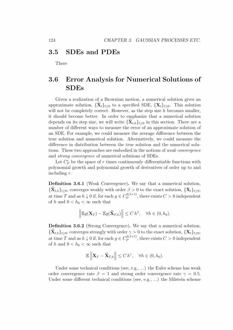
124 CHAPTER 3. GAUSSIAN PROCESSES ETC.
3.5 SDEs and PDEs
There
3.6 Error Analysis for Numerical Solutions of
SDEs
Given a realization of a Brownian motion, a numerical solution gives anapproximate solution, Xtt≥0 to a specified SDE, Xtt≥0. This solutionwill not be completely correct. However, as the step size h becomes smaller,it should become better. In order to emphasize that a numerical solutiondepends on its step size, we will write Xt,ht≥0 in this section. There are anumber of different ways to measure the error of an approximate solution ofan SDE. For example, we could measure the average difference between thetrue solution and numerical solution. Alternatively, we could measure thedifference in distribution between the true solution and the numerical solu-tions. These two approaches are embodied in the notions of weak convergenceand strong convergence of numerical solutions of SDEs.
Let CrP be the space of r times continuously differentiable functions with
polynomial growth and polynomial growth of derivatives of order up to andincluding r.
Definition 3.6.1 (Weak Convergence). We say that a numerical solution,
Xt,ht≥0, converges weakly with order β > 0 to the exact solution, Xtt≥0,
at time T and as h ↓ 0 if, for each g ∈ C2(β+1)P , there exists C > 0 independent
of h and 0 < h0 < ∞ such that
∥∥∥Eg(XT )− Eg(XT,h)∥∥∥ ≤ C hβ, ∀h ∈ (0, h0).
Definition 3.6.2 (Strong Convergence). We say that a numerical solution,
Xt,ht≥0, converges strongly with order γ > 0 to the exact solution, Xtt≥0,
at time T and as h ↓ 0 if, for each g ∈ C2(β+1)P , there exists C > 0 independent
of h and 0 < h0 < ∞ such that
E
∥∥∥XT − XT,h
∥∥∥ ≤ C hγ, ∀h ∈ (0, h0).
Under some technical conditions (see, e.g., ...) the Euler scheme has weakorder convergence rate β = 1 and strong order convergence rate γ = 0.5.Under some different technical conditions (see, e.g., ...) the Milstein scheme

3.6. ERROR ANALYSIS FOR NUMERICAL SOLUTIONS OF SDES 125
has weak order convergence rate β = 1 and strong order convergence rateγ = 1.
In general, in Monte Carlo we are interested in estimating expectations.This means that weak order convergence is usually the relevant convergenceconcept. It is important to bear this in mind. Although the Milstein schemeappears better, it involves calculating derivatives (sometimes these can bedone by hand in advance, but sometimes they need to be done numerically).This imposes an additional cost which may not be worth it if strong orderconvergence is not important.
Example 3.6.3. Consider the SDE for geometric Brownian motion
dXt = µXt dt+ σXt dWt.
This has the exact solution
Xt = X0 exp
(µ− σ2
2
)t+ σWt
.
For a given realization of Wtt∈[0,1], we can compare the numerical solu-tions with the exact solutions. The following code generates a realizationof Brownian motion (at a fixed number of points) and then plots the Eulerand Milstein approximations against the exact solution for a number of meshsizes.
Listing 3.14: Matlab code
1 L = 4; m_max = 2^L;
2 mu = 0.1; sigma = 0.2; X_0 = 1;
3
4 Z = randn(m_max,1);
5
6 for l = 1:L
7 m = 2^l; h = 1/m;
8 Z_coarse = zeros(m,1);
9 X_eul = zeros(1,m+1); X_eul(1) = X_0;
10 X_mil = zeros(1,m+1); X_mil(1) = X_0;
11 X = zeros(1,m+1); X = X_0;
12
13 for k = 1:m
14 Z_coarse(k) = 1/sqrt(2^(L-l))...
15 *sum(Z((k-1)*2^(L - l)+1:k*2^(L - l)));
16 end
17 W_coarse = sqrt(h) * cumsum(Z_coarse);
18 for i = 2:m+1

126 CHAPTER 3. GAUSSIAN PROCESSES ETC.
19 X_eul(i) = X_eul(i-1) + mu*X_eul(i-1)*h ...
20 + sigma*X_eul(i-1)*sqrt(h)*Z_coarse(i-1);
21 X_mil(i) = X_mil(i-1) + mu*X_mil(i-1)*h ...
22 + sigma*X_mil(i-1)*sqrt(h)*Z_coarse(i-1)...
23 + sigma^2 * X_mil(i-1) * h/2 * (Z_coarse(i-1)^2 - 1);
24 X(i) = X_0...
25 *exp((mu - sigma^2 / 2)*((i-1)*h) + sigma*W_coarse(i-1));
26 end
27 figure(l); hold on;
28 plot(0:h:1,X,’black’)
29 plot(0:h:1,X_eul,’red’)
30 plot(0:h:1,X_mil,’blue’)
31 legend(’Exact’,’Euler Approximation’,’Milstein Approximation’)
32 end
0 0.1 0.2 0.3 0.4 0.5 0.6 0.7 0.8 0.9 11
1.1
1.2
1.3
1.4
1.5
1.6
1.7
1.8
ExactEuler ApproximationMilstein Approximation
Figure 3.6.1: Plots of the exact solution, Euler approximation and Mil-stein approximation of geometric Brownian motion for a fixed realizationof Wtt∈[0,1] with mesh size h = 1/2
As we have often seen, the common object of interest in Monte Carlo isestimating ℓEf(X), where X is a random vector. In the case of SDEs, X isoften XT , the value of the solution of an SDE at time T . There are other,more complicated, things that we might wish to estimate, such as functionalsof paths of SDEs. However, I will not focus too much on these.
If we wish to estimate ℓ = Ef(XT ), we generally use the standard Monte

3.6. ERROR ANALYSIS FOR NUMERICAL SOLUTIONS OF SDES 127
0 0.1 0.2 0.3 0.4 0.5 0.6 0.7 0.8 0.9 11
1.1
1.2
1.3
1.4
1.5
1.6
1.7
1.8
ExactEuler ApproximationMilstein Approximation
Figure 3.6.2: Plots of the exact solution, Euler approximation and Mil-stein approximation of geometric Brownian motion for a fixed realizationof Wtt∈[0,1] with mesh size h = 1/4
0 0.1 0.2 0.3 0.4 0.5 0.6 0.7 0.8 0.9 11
1.1
1.2
1.3
1.4
1.5
1.6
1.7
1.8
ExactEuler ApproximationMilstein Approximation
Figure 3.6.3: Plots of the exact solution, Euler approximation and Mil-stein approximation of geometric Brownian motion for a fixed realizationof Wtt∈[0,1] with mesh size h = 1/8

128 CHAPTER 3. GAUSSIAN PROCESSES ETC.
0 0.1 0.2 0.3 0.4 0.5 0.6 0.7 0.8 0.9 1
1
1.2
1.4
1.6
1.8
ExactEuler ApproximationMilstein Approximation
Figure 3.6.4: Plots of the exact solution, Euler approximation and Mil-stein approximation of geometric Brownian motion for a fixed realizationof Wtt∈[0,1] with mesh size h = 1/16
Carlo estimator
ℓ =1
N
N∑
i=1
f(X
(i)T,h
),
where X(1)T,h, . . . ,X
(N)T,h are iid copies of the numerical solution of with mesh
size h. In general, this estimator is biased. This is because both the Eulerand Milstein schemes are biased. This means that we should measure itserror using MSE. Remember that the MSE of an estimator is of the form
MSE(ℓ) = Var(ℓ) + Bias(ℓ)2.
The two parts of the MSE correspond to different types of error: statistical
error and approximation error. The statistical error, measured by the vari-ance, comes from the fact that there are an uncountably infinite number ofpaths of Brownian motion and we are only sampling a small number. Theapproximation error, measured by the bias, comes from the fact that givena realization of a Brownian path, we still only get an approximate solutionto our SDE.
If we think a little harder, we can write the MSE as
MSE(ℓ) = Var(XT,h) +∥∥∥Ef(XT )− Ef(XT,h)
∥∥∥2
.
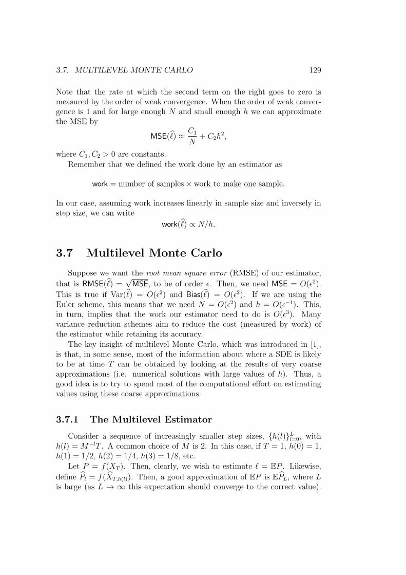
3.7. MULTILEVEL MONTE CARLO 129
Note that the rate at which the second term on the right goes to zero ismeasured by the order of weak convergence. When the order of weak conver-gence is 1 and for large enough N and small enough h we can approximatethe MSE by
MSE(ℓ) ≈ C1
N+ C2h
2,
where C1, C2 > 0 are constants.
Remember that we defined the work done by an estimator as
work = number of samples× work to make one sample.
In our case, assuming work increases linearly in sample size and inversely instep size, we can write
work(ℓ) ∝ N/h.
3.7 Multilevel Monte Carlo
Suppose we want the root mean square error (RMSE) of our estimator,
that is RMSE(ℓ) =√MSE, to be of order ǫ. Then, we need MSE = O(ǫ2).
This is true if Var(ℓ) = O(ǫ2) and Bias(ℓ) = O(ǫ2). If we are using theEuler scheme, this means that we need N = O(ǫ2) and h = O(ǫ−1). This,in turn, implies that the work our estimator need to do is O(ǫ3). Manyvariance reduction schemes aim to reduce the cost (measured by work) ofthe estimator while retaining its accuracy.
The key insight of multilevel Monte Carlo, which was introduced in [1],is that, in some sense, most of the information about where a SDE is likelyto be at time T can be obtained by looking at the results of very coarseapproximations (i.e. numerical solutions with large values of h). Thus, agood idea is to try to spend most of the computational effort on estimatingvalues using these coarse approximations.
3.7.1 The Multilevel Estimator
Consider a sequence of increasingly smaller step sizes, h(l)Ll=0, withh(l) = M−lT . A common choice of M is 2. In this case, if T = 1, h(0) = 1,h(1) = 1/2, h(2) = 1/4, h(3) = 1/8, etc.
Let P = f(XT ). Then, clearly, we wish to estimate ℓ = EP . Likewise,
define Pl = f(XT,h(l)). Then, a good approximation of EP is EPL, where Lis large (as L → ∞ this expectation should converge to the correct value).

130 CHAPTER 3. GAUSSIAN PROCESSES ETC.
Now, observe that we can write EPL as
EPL = EP0 +L∑
l=1
(EPl − EPl−1
)
= EP0 +L∑
l=1
E(Pl − Pl−1)
We can estimate these using independent estimators for each summand,which are defined by
EP0 ≈ Y0 =1
N0
N0∑
i=1
f(X
(i)T,h(0)
)
and, for l = 1, . . . , L,
E(Pl − Pl−1) ≈ Yl =1
Nl
Nl∑
i=1
[f(X
(i)T,h(l)
)− f
(X
(i)T,h(l−1)
)],
where, very importantly, X(i)T,h(l) and X
(i)T,h(l−1) are generated using the same
realization of Brownian motion. Then, EPL can be estimated by Y (L), where
Y (L) = Y0 +L∑
l=1
Yl.
3.7.2 Variance, Work and Optimal Sample Sizes
The variance of the estimator is given by
Var(Y (L)) = Var
(Y0 +
L∑
l=1
Yl
)=
L∑
l=0
Vl
Nl
,
where V0 = Var(f(XT,h(0))) and, for l = 1, . . . , L,
Vl = Var(f(XT,h(l))− f(XT,h(l−1))
).
We can write work done by this estimator in terms of the various samplesizes and step sizes as
work(Y (L)) ∝L∑
l=0
Nl
hl
.

3.7. MULTILEVEL MONTE CARLO 131
Taking a fixed work budget, proportional to W , and assuming that we do notneed integer sample sizes (rounding afterwards should more or less preserveoptimality), we can find the optimal sample sizes using standard calculus.We solve
∇N
(L∑
l=0
Vl
Nl
+ λ
(L∑
l=0
Nl
hl
−W
))= 0
to get
Nl =
√Vlhl
λ∝√
Vlhl.
3.7.3 A Rough Sketch of Why Multilevel Monte CarloWorks
If we use the Euler scheme, we have that, as h → 0,
E
[Pl − P
]= O(hl),
as this is measured using weak convergence. Likewise, we have
E
∥∥∥XT − XT,h(l)
∥∥∥ = O(h1/2) → E
∥∥∥XT − XT,h(l)
∥∥∥2
= O(h)
by strong convergence. We will assume f is Lipschitz, which means thatthere exists C > 0 such that
‖f(x)− f(y)‖ ≤ C ‖x− y‖ ,
for all x and y in the domain of f . This is a very strong assumption, which isrelaxed in the general theorem. However, it makes the calculations relativelystraightforward. Now, observe that
Var(Pl − P
)= E
(Pl − P
)2−(EPl − P
)2≤ E
(Pl − P
)2
= E
∥∥∥f(XT,h(l))− f(XT )∥∥∥2
≤ C∥∥∥XT,h(l) −XT
∥∥∥2
= O(hl).
We can obtain an upper bound on the variance of Pl − Pl−1 by writing
Pl − Pl−1 =(Pl − P
)+(P − Pl−1
)
and observing that
Var(Pl − Pl−1
)≤(√
Var(Pl − P
)+
√Var
(P − Pl−1
))2
= O(hl)

132 CHAPTER 3. GAUSSIAN PROCESSES ETC.
Now, choosing Nl = O(ǫ−2Lhl) we get
Var(Y (L)) =L∑
l=0
Vl
Nl
=L∑
l=1
O(hl)
O(ǫ−2Lhl)= O(ǫ−2).
If we then choose
L =log ǫ−1
logM+O(1)
as ǫ → 0, then hL = O(ǫ). This implies that we have MSE = O(ǫ2) with
work ∝L∑
l=0
Nl
hl
=L∑
l=0
O(ǫ−2Lhl)
hl
= O(ǫ−2L2) = O(ǫ−2(log ǫ)2),
which is better than standard Monte Carlo.
3.7.4 The Key Theorem
The following theorem, first established in [1], gives quite general re-sults under which the multilevel approach works well. For more details,extensions, and other applications, take a look at Mike Giles’ website (go tohttp://people.maths.ox.ac.uk/~gilesm/).
Theorem 3.7.1. Let P denote a functional of the solution of
dXt = a(Xt, t) dt+ b(Xt, t) dWt,
for a given Brownian path Wtt≥0 and let Pl denote the corresponding ap-proximation using a numerical discretization with timestep h(l) = M−lT . If
there exist independent estimators Yl based on Nl Monte Carlo samples andpositive constants α ≥ 1/2, β, c1, c2, c3 such that
(i) E[Pl − P ] ≤ c1hαl ,
(ii) EYl =
EP0, l = 0,
E[Pl − Pl−1], l > 0,
(iii) Var(Yl) ≤ c2N−1l hβ
l ,
(iv) Cl, the computational complexity of Yl is bounded by
Cl ≤ c3Nlh−1l ,

3.7. MULTILEVEL MONTE CARLO 133
then there exists a positive constant c4 such that for any ǫ > e−1, there arevalues L and Nl for which the multilevel estimator
Y =L∑
l=0
Yl
has an MSE with boundMSE < ǫ2,
with computational complexity C with bound
C ≤
c4ǫ−2, β > 1,
c4ǫ−2(log ǫ)2, β = 1,
c4ǫ−2−(1−β)/α, 0 < β < 1.
Proof. See [1]
3.7.5 Implementation
Listing 3.15: Matlab code
1 mu = 0.1; sigma = 0.05;
2 X_0 = 1; L = 6; Y = zeros(L,1);
3
4 N_0 = 10^(L+1); N = zeros(L,1);
5
6 for l = 1:L
7 N(l) = 10^(L+1-l);
8 end
9
10 m = 1; h = 1;
11 vals = zeros(N_0,1);
12
13 for i = 1:N_0
14 X = X_0;
15 for k = 1:m
16 X = X + mu*X*h + sigma*X*sqrt(h)*randn;
17 end
18 vals(i) = X;
19 end
20
21 Y_0 = mean(vals);
22
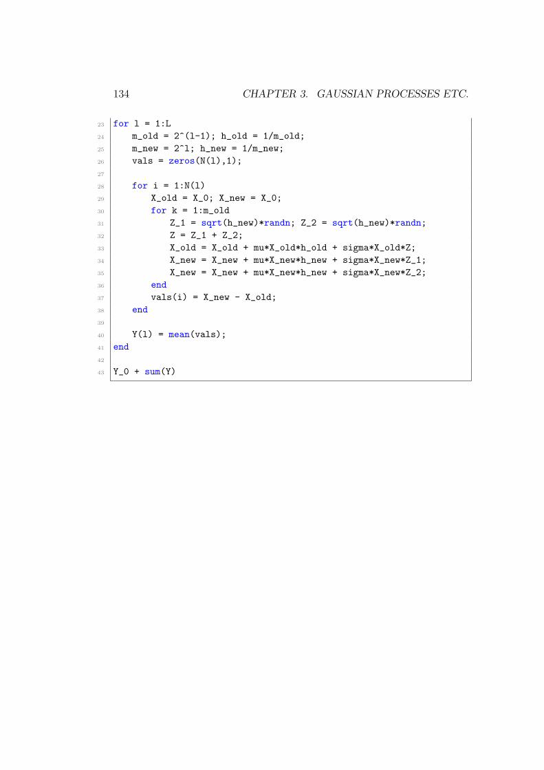
134 CHAPTER 3. GAUSSIAN PROCESSES ETC.
23 for l = 1:L
24 m_old = 2^(l-1); h_old = 1/m_old;
25 m_new = 2^l; h_new = 1/m_new;
26 vals = zeros(N(l),1);
27
28 for i = 1:N(l)
29 X_old = X_0; X_new = X_0;
30 for k = 1:m_old
31 Z_1 = sqrt(h_new)*randn; Z_2 = sqrt(h_new)*randn;
32 Z = Z_1 + Z_2;
33 X_old = X_old + mu*X_old*h_old + sigma*X_old*Z;
34 X_new = X_new + mu*X_new*h_new + sigma*X_new*Z_1;
35 X_new = X_new + mu*X_new*h_new + sigma*X_new*Z_2;
36 end
37 vals(i) = X_new - X_old;
38 end
39
40 Y(l) = mean(vals);
41 end
42
43 Y_0 + sum(Y)
Chapter 4
Spatial Processes
4.1 Random Fields
At the beginning of these notes we defined a stochastic process as a setof random variables Xii∈I taking values in a state space X with indexset I ⊂ R. It seems natural to ask what would happen if we took I to besomething “larger” than a subset of R — for example, a subset of RN . Suchgeneralizations are called random fields. Intuitively, we can think of themas stochastic processes evolving over space instead of time. Sometimes, theycan be thought of as spatial processes that are also evolving over time (forexample, if I = [a, b]3 × [0, T ]).
Definition 4.1.1 (Random Field). Let I ⊂ RN and Xii∈I be a set of d-
dimensional random vectors indexed by I. We say Xii∈I is a (N, d) randomfield.
Note that stochastic processes are random fields.
4.1.1 Gaussian Random Fields
Some of the simplest random fields to work with are Gaussian random
fields. These are a natural extension of our definition of Gaussian processes.
Definition 4.1.2. A random field Xii∈I is a Gaussian random field if(Xi1 , . . . , Xin) has a multivariate normal distribution for all 1 ≤ n < ∞ and(i1, . . . , in) ∈ In.
As with Gaussian processes, we can describe the finite dimensional dis-tributions of Gaussian random fields using a mean function µ(i) = EXi anda covariance function r(i, j) = Cov(Xi, Xj). If we wish to consider the Gaus-sian random field at a finite number of points, we can treat its values as a
135

136 CHAPTER 4. SPATIAL PROCESSES
random vector. We can use the mean function and covariance function toconstruct the mean vector, µ, and covariance matrix, Σ, of these points.
Using these functions, and treating a finite number of points of the ran-dom field as a vector, we can generate a realization of the field
Example 4.1.3 (Gaussian White Noise). A trivial example of a Gaussianrandom field is Gaussian white noise. On I = 1, . . . ,m × 1, . . . ,m, thisis the process, Xii∈I with mean function
µ(i) = EXi = 0,
and covariance function
r(i, j) = r((xi, yi), (xj, yj)) = Cov(X(xi,yi), X(xj ,yj)) =
1 if (xi, yi) = (xj, yj)
0 otherwise.
We can simulate this in Matlab by simple generating a matrix of standard
10 20 30 40 50 60 70 80 90 100
10
20
30
40
50
60
70
80
90
100
Figure 4.1.1: A realization of Gaussian white noise
normal random variables.
Listing 4.1: Matlab code
1 m = 100;
2 Z = randn(m,m);
3 imagesc(Z);
4 colormap(gray);

4.1. RANDOM FIELDS 137
Example 4.1.4 (Brownian Sheet). The Brownian sheet, W(x,y)(x,y)∈[0,1]2 isa natural random field extension of Brownian motion on [0, 1]. It has meanfunction
µ(i) = EXi = 0,
and covariance function
r(i, j) = r((xi, yi), (xj, yj)) = Cov(W(xi,yi),W(xj ,yj)) = min(xi, xj)min(yi, yj).
00.2
0.40.6
0.81
00.2
0.40.6
0.81
−0.5
0
0.5
1
1.5
2
Figure 4.1.2: A realization of a Brownian sheet
We can easily simulate this in Matlab.
Listing 4.2: Matlab code
1 alpha = 1.5; x = .01:.01:1; y = .01:.01:1;
2
3 n1 = length(x); n2 = length(y);
4
5 Sigma = zeros(n1*n2,n1*n2);
6
7 for i = 1:n2
8 for j = 1:n1
9 row_state = (i-1)*n2 + j;
10 for k = 1:n2
11 for l = 1:n1
12 column_state = (k-1)*n2 + l;
13 Sigma(row_state,column_state) = ...
138 CHAPTER 4. SPATIAL PROCESSES
14 min(x(j),x(l))*min(y(i),y(k));
15 end
16 end
17 end
18 end
19
20 A = chol(Sigma);
21 Y = randn(1,n1*n2) * A;
22
23 X = zeros(n1,n2);
24
25 for i = 1:n2
26 for j = 1:n1
27 X(i,j) = Y((i-1)*n2 + j);
28 end
29 end
30
31 surf(x,y,X)
Random fields are, in general, difficult to work with. For that reason, itis nice to identify classes of random fields that are more tractable.
Definition 4.1.5 (Stationarity). We say a random field, Xii∈I , is station-ary if (Xi1 , . . . , Xin) has the same distribtion as (Xi1+s, . . . , Xin+s) for alln ≥ 1, (i1, . . . , in) ∈ In and s ∈ I.
Weak stationary implies that the first two moments of the distributionsdo not change.
Definition 4.1.6 (Wide sense (weak) stationarity). A random field, Xii∈Iis wide-sense stationary if µ(i) = c for all i ∈ I and r(i, j) = r(|i− j|). Thatis, the covariance function is simply a function of the displacement vectorbetween the points i and j.
Analogously to the case of Gaussian processes, Gaussian fields are station-ary if they are weak stationary. When considering random fields, a differenttype of invariance property is also useful. This is called isotropy. Basically,this means the distribution of the object does not change when the object isrotated. We will only consider a very special case of isotropy.
Definition 4.1.7 (Stationary wide sense isotropy). A stationary randomfield is wide sense isotropic if r(i, j) = r(‖i − j‖). That is, the covariancebetween points i and j only depends on the distance between them.
Note that non-stationary random fields can be isotropic.

4.1. RANDOM FIELDS 139
4.1.2 Markov Random Fields
When considering stochastic processes, the Markov property simplifiedthings considerably. Markov random fields are the random field analogues ofMarkov stochastic processes. To define a meaningful version of the Markovproperty, we exploit the idea of conditional independence.
Definition 4.1.8 (Conditional Independence for Events). We say two eventsA and B are said to be conditionally independent given C if
P(A ∩ B |C) = P(A |C)P(B |C).
Clearly, a Markov process is conditional independent of its past given itspresent.
Definition 4.1.9 (Conditional Independence for Random Variables). Wecan easily extend this definition to random vectors X,Y and Z with jointdensity π(x,y, z). We say X and Y are conditionally independent given Z(denoted x⊥y | z) if
π(x,y | z) = π(x | z)π(y | z).There is a nice criterion for determining conditional independence given
a joint density.
Theorem 4.1.10 (Factorization Theorem). Given random vectors X,Y andZ with joint density π(x,y, z), we say x⊥y | z if and only if
π(x,y, z) = f(x, z)g(y, z)
for some functions f and g and all z with π(z) > 0.
Example 4.1.11. Take
π(x, y, z) ∝ expx+ xz + yzon some bounded region. We can write
π(x, y, z) ∝ expx+ xzexpyz = f(x, z)g(y, z)
so x⊥y | z.Example 4.1.12. Take
π(x, y, z) ∝ expxyzon some bounded region. We cannot factorize this into a function of x andz and a function of y and z, so x and y are not conditionally independentgiven z here.

140 CHAPTER 4. SPATIAL PROCESSES
We can represent conditional dependence relations using graphs calledgraphical models.
Example 4.1.13.
PICTURE HERE
This example encodes the dependency structure
π(a, b, c, d) = π(a)π(b)π(c | b, d)π(d | a, b, c).
Markov random fields depict a specific dependency structure using undi-rected graphs G = (V,E). Alternatively, you can think of these as graphswith arrows on both ends of the edges.
PICTURE HERE
In Markov random fields, random variables are conditionally independentof the rest of the graph given their immediate neighbors.
Definition 4.1.14 (Neighbors of a Vertex). The neighbors of the vertex iare the members of the set
Ni = j ∈ V : (i, j) ∈ E.
For example, in the graph above, N1 = 2, 3, N2 = 1, 3, 4, N3 =1, 2, 4 and N4 = 2, 3.
We can now define a Markov random field. It will be convenient to useto following notation. For C ⊂ V , let XC = Xi : i ∈ C and X−C = Xi :i ∈ V \ C.
Definition 4.1.15 (Markov Random Field). We say a sequence of randomvariables, X = Xii∈V , indexed by the vertices of G = (V,E), is a Markovrandom field if Xi |X−i has the same distribution as Xi |XNi
for all i ∈ V .
4.1.3 Gaussian Random Markov Fields
We will consider a special class of Markov random fields, called Gaussian
random Markov fields.
Definition 4.1.16 (Gaussian Random Markov Field). A Gaussian randomMarkov field (GRMF) is a Markov random field which is also a Gaussianfield.

4.1. RANDOM FIELDS 141
010
2030
4050
0
20
40
60−5
0
5
10
Figure 4.1.3: A realization of a Gaussian Markov random field on a 50× 50lattice
We will assume that the GRMFs we consider have densities. That is,the covariance matrix of a finite number of points, Σ, will always be positivedefinite. Recall that the pdf of a normal vector X is given by
f(x;µ,Σ) = (2π)−n/2 |Σ|−1/2 exp
−1
2(x− µ)⊺Σ−1(x− µ)
.
In general, the covariance matrix is a natural object to consider whentalking about Gaussian processes and fields. However, in the case of Gaussianrandom fields, it turns out that the precision matrix is a more natural objectto work with.
Definition 4.1.17 (Precision Matrix). The precision matrix, Q, of a covari-ance matrix, Σ, is its inverse. That is,
Q = Σ−1.
We can rewrite the pdf of a normal vector in terms of its precision matrixas
f(x;µ, Q) = (2π)−n/2 |Q|1/2 exp−1
2(x− µ)⊺Q(x− µ)
.
The following result reveals the reason why precision matrices are soappealing when working with GRMFs.
142 CHAPTER 4. SPATIAL PROCESSES
Theorem 4.1.18. Let X be normally distributed with mean µ and precisionmatrix Q. Then, for i 6= j,
Xi⊥Xj |X−i,j ⇐⇒ Qi,j = 0.
Proof. Assume without loss of generality that µ = 0. We have
π(x) ∝ exp
−1
2x⊺Qx
= exp
−1
2
∑
l∈V
∑
k∈V
xkQk,lxl
= exp
−1
2xixj(Qi,j +Qj,i)−
1
2
∑
k,l6=i,j
xkQk,lxl
If you consider examples 4.1.12 and 4.1.13, then it is clear that this pdf canonly be factorized in the necessary way if Qi,j = Qj,i = 0.
Theorem 4.1.19. Let X be a GRMF with respect to G = (V,E) with meanµ and precision matrix Q. Then,
(i) E [Xi |X−i] = µi − 1Qi,i
∑j∈Ni
Qi,j(Xj − µj).
(ii) Prec(Xi |X−i) = Qii.
(iii) Corr(Xi, Xj |Xi,j) =−Qi,j√Qi,iQj,j
.
Theorem 4.1.20. Let X be a GRMF with respect to G = (V,E). Then,the following are equivalent:
(i) The pairwise Markov property
Xi⊥Xj |X−i,j (i, j) /∈ E, i 6= j.
(ii) The local Markov property
Xi⊥X−i∪Ni|XNi
∀i ∈ V.
(iii) The global Markov property
XA⊥XB |XC
for all disjoint A,B and C, where C separates A and B.

4.1. RANDOM FIELDS 143
GRMFs are very appealing from a computational perspective as the pre-cision matrix Q is sparse (that is, it is mostly zeros). In general, matrixoperations are much faster for sparse matrices. In addition, far less memoryis required in order to store sparse matrices.
Remember that the inverse of a SPD matrix is also SPD. This impliesthat Q has a Cholesky decomposition. We can use this to generate normalrandom vectors with the desired distributions.
Theorem 4.1.21. Given a SPD covariance matrix Σ and a vector µ, therandom vector
X = µ+ (C⊺)−1 Z ∼ N(µ,Σ),
where C is such that Σ−1 = Q = CC⊺ and Z ∼ N(0, I).
Proof. We know X is multivariate normal, so we just need to check that ithas the correct mean and variance. Now,
E[µ+ (C⊺)−1 Z
]= µ+ (C⊺)−1
EZ = µ,
and
Var(µ+ (C⊺)−1 Z
)= (C⊺)−1 Var(Z) (C)−1 = (CC⊺)−1 = Q−1 = Σ.
Example 4.1.22 (A Gaussian random Markov field on a Lattice). We sim-ulate a zero mean GRMF on the 200 × 200 square lattice with Qi,i = 1and
Qi,j =
−0.25 if (i, j) ∈ E
0 otherwise.
Listing 4.3: Matlab code
1 m = 200; d1 = 1; d2 = -0.25;
2 nels = m*(5*m-4);
3
4 a = zeros(1, nels); b = zeros(1,nels); q = zeros(1,nels);
5 %compute the links and weights for the precision matrix
6 k=0;
7 for i=1:m
8 for j=1:m
9 A = findneigh(i,j,m);
10 number_neighbours = size(A,1);
11 for h=1:number_neighbours
12 a(k+h)= ij2k(i,j,m);

144 CHAPTER 4. SPATIAL PROCESSES
13 b(k+h)= ij2k(A(h,1),A(h,2),m);
14 if h==1
15 q(k+h) = d1;
16 else
17 q(k+h) = d2;
18 end
19 end
20 k = k+number_neighbours;
21 end
22 end
23 %construct the precision matrix
24 Q = sparse(a,b,q,m^2,m^2);
25 %calculate the Cholesky matrix
26 C = chol(Q,’lower’);
27 Z = randn(m^2,1);
28 % generate the Gaussian process
29 x = C\Z;
30 colormap gray, brighten(-0.2)
31 imagesc(reshape(x,m,m)) % plot the result
This uses the following functions.
Listing 4.4: Matlab code
1 function A = findneigh(i,j,m)
2 % find neighbors of the (i,j)-th site of an m by m square lattice
3 if i==1
4 if j==1
5 A = [1,1;1,2;2,1];
6 elseif j==m
7 A = [1,m;1,m-1;2,m];
8 else
9 A = [1,j;1,j-1;1,j+1;2,j];
10 end
11 elseif i==m
12 if j==1
13 A = [m,1;m,2;m-1,1];
14 elseif j==m
15 A = [m,m;m,m-1;m-1,m];
16 else
17 A = [m,j;m,j-1;m,j+1;m-1,j];
18 end
19 else
20 if j==1
21 A = [i,1;i,2;i-1,1;i+1,1];

4.2. SPATIAL POISSON PROCESSES 145
22 elseif j==m
23 A = [i,m;i,m-1;i+1,m;i-1,m];
24 else
25 A = [i,j;i,j-1;i,j+1;i+1,j;i-1,j];
26 end
27 end
28 end
Listing 4.5: Matlab code
1 function k = ij2k(i,j,m)
2 k = (i-1)*m + j;
20 40 60 80 100 120 140 160 180 200
50
100
150
200
Figure 4.1.4: A realization of the random field
4.2 Spatial Poisson Processes
We want to extend the notion of a Poisson process, which we have alreadydiscussed in 1 dimension, to higher dimensions. Remember, we defined thisprocess in three equivalent ways: the arrival times, the inter-arrival times,and the counting process Ntt≥0. It no longer makes sense to think aboutinter-arrival times, but if we think of the arrival times as positions in space(on the 1D line) then it is clear that we can possibly extend this definition tospace. As it turns out, however, the counting function definition is in somesense the nicest method of extending the Poisson process to space.

146 CHAPTER 4. SPATIAL PROCESSES
Think of the function N([a, b]) = Nb −Na. This measures the number ofpoints in the bounded set [a, b]. Such a measure is called a counting measure.If we know the locations of the points, it is easy to construct this function.Conversely, if we know the function we can find the location of the points.
In the following, we will use νd to denote d-dimensional Lebesgue measure.
4.2.1 Binomial Process
Consider a bounded windowW ⊂ Rd with a single point placed uniformly
in it. The location of this point, x, has the probability density
f(x) =
1
νd(W )if x ∈ W
0 otherwise.
If we consider a bounded set B ⊂ Rd, then, for X, the point we randomly
threw into W , we have
P(X ∈ B) =
∫
B
f(x) dx =νd(B ∩W )
νd(W ).
If we throw n points into W , then we have a binomial process.
Definition 4.2.1. A binomial point process of n points is a process of nindependent points, X1, . . . ,Xn, uniformly distributed in the bounded setW .
If we consider N(B), the number of points in some bounded set B, thenthis can be written as
N(B) =n∑
i=1
I(Xi ∈ B).
It is straightforward to see that N(B) has a binomial distribution. Specifi-cally, N(B) ∼ Bin(n, p), where p = P(X ∈ B), defined above.
It is straightforward to generate a binomial process. The only difficultylies in generating points uniformly in the set W . This is primarily difficult inhigh dimensions but, in practice, may not be such an issue as the dimensionof a point process is usually quite low.
Here is an example in two dimensions.
Listing 4.6: Matlab code
1 n = 20; dims = [0 10; 0 10];
2

4.2. SPATIAL POISSON PROCESSES 147
3 X = zeros(n,2);
4
5 X(:,1) = (dims(1,2) - dims(1,1)) * rand(n,1);
6 X(:,2) = (dims(2,2) - dims(2,1)) * rand(n,1);
7
8 S = 200 * ones(n,1);
9 scatter(X(:,1),X(:,2),S,’fill’)
Here is an example in three dimensions.
Listing 4.7: Matlab code
1 n = 20; dims = [0 10; 0 10; 0 10];
2
3 X = zeros(n,3);
4
5 X(:,1) = (dims(1,2) - dims(1,1)) * rand(n,1);
6 X(:,2) = (dims(2,2) - dims(2,1)) * rand(n,1);
7 X(:,3) = (dims(3,2) - dims(3,1)) * rand(n,1);
8
9 S = 200 * ones(n,1);
10 scatter3(X(:,1),X(:,2),X(:,3),S,’fill’)
0 2 4 6 8 100
2
4
6
8
10
Figure 4.2.1: A realization of a binomial process on [0, 10] × [0, 10] withn = 20 points.
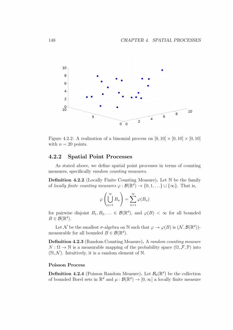
148 CHAPTER 4. SPATIAL PROCESSES
02
46
810
0
5
100
2
4
6
8
10
Figure 4.2.2: A realization of a binomial process on [0, 10] × [0, 10] × [0, 10]with n = 20 points.
4.2.2 Spatial Point Processes
As stated above, we define spatial point processes in terms of countingmeasures, specifically random counting measures.
Definition 4.2.2 (Locally Finite Counting Measure). Let N be the familyof locally finite counting measures ϕ : B(Rd) → 0, 1, . . . ∪ ∞. That is,
ϕ
(∞⋃
n=1
Bn
)=
∞∑
n=1
ϕ(Bn)
for pairwise disjoint B1, B2, . . . ∈ B(Rd), and ϕ(B) < ∞ for all boundedB ∈ B(Rd).
Let N be the smallest σ-algebra on N such that ϕ → ϕ(B) is (N ,B(Rd))-measurable for all bounded B ∈ B(Rd).
Definition 4.2.3 (Random Counting Measure). A random counting measure
N : Ω → N is a measurable mapping of the probability space (Ω,F ,P) into(N,N ). Intuitively, it is a random element of N.
Poisson Process
Definition 4.2.4 (Poisson Random Measure). Let B0(Rd) be the collection
of bounded Borel sets in Rd and µ : B(Rd) → [0,∞] a locally finite measure

4.2. SPATIAL POISSON PROCESSES 149
(i.e., µ(B) < ∞ for all B ∈ B0(Rd)). We say NBB∈B(Rd) is a Poisson
random measure with intensity measure µ if
(i) NB1 , NB2 , . . . are independent random variables for pairwise disjointB1, B2 . . . ∈ B0(R
d).
(ii) NB ∼ Poi(µ(B)) for all B ∈ B0(Rd).
If µ is proportion to νd (i.e., µ(B) = λνd(B) for all B ∈ B(Rd)), thenNBB∈B(Rd) is said to be a homogenous Poisson counting measure with in-tensity λ.
Lemma 4.2.5. Consider a Poisson point process in Rd with constant inten-
sity λ > 0. Let W ⊂ Rd be a region with 0 < νd(W ) < ∞. Given N(W ) = n,
the conditional distribution of N(B) for B ⊆ W is binomial, with
P(N(B) = k |N(W ) = n) =
(n
k
)pk(1− p)n−k,
where p = νd(B)/νd(W ). Furthermore, the conditional joint distribution ofN(B1), . . . , N(Bn) for any B1, . . . , Bn ⊂ W is the same as the joint distribu-tion of these random variables for a binomial process.
Proof. Let 0 ≤ k ≤ n. Then
P(N(B) = k |N(W ) = n) =P(N(B) = k,N(W ) = n)
P(N(W ) = n)
=P(N(B) = k,N(W \B) = n− k)
P(N(W ) = n)
=P(N(B) = k)P(N(W \B) = n− k)
P(N(W ) = n)
=e−λνd(B) (λνd(B))k
k!e−λνd(W\B) (λνd(W\B))n−k
(n−k)!
e−λνd(W ) (λνd(W ))n
n!
=
(n
k
)(νd(B)
νd(B)
)k (1− νd(B)
νd(B)
)n−k
.
Lemma 4.2.5 suggests that we can simulate a homogenous Poisson pro-cess on W be generating N(W ) ∼ Poi(λνd(W )), then simulating a binomialprocess with N(W ) points.

150 CHAPTER 4. SPATIAL PROCESSES
Example 4.2.6. Consider a homogenous Poisson process on W = (x, y) :x2 + y2 ≤ 1 with λ = 100. We can simulate this as follows.
Listing 4.8: Matlab code
1 lambda = 100; N = poissrnd(lambda * pi);
2 X = zeros(N,2); count = 1;
3
4 while count <= N
5 x = 2*rand - 1; y = 2 * rand - 1;
6 if (x^2 + y^2) <= 1
7 X(count,1) = x;
8 X(count,2) = y;
9 count = count + 1;
10 end
11 end
12
13 S = 200 * ones(N,1);
14 scatter(X(:,1),X(:,2),S,’fill’)
−1 −0.5 0 0.5 1−1
−0.5
0
0.5
1
Figure 4.2.3: A realization of a Poisson process with constant intensity λ =100 on W = (x, y) : x2 + y2 ≤ 1.
Inhomogeneous Poisson Processes
Inhomogeneous Poisson processes (i.e. processes where it is not true thatµ(B) = λνd(B) for all B ∈ B(Rd)) are at little more challenging to simulate

4.2. SPATIAL POISSON PROCESSES 151
and work with than homogeneous Poisson processes. We will restrict ourattention to processes with measures that are absolutely continuous withrespect to d-dimensional Lebesgue measure. For such processes, there existsa Borel measurable function λ : Rd → [0,∞) such that
µ(B) =
∫
B
λ(x) dx
for all B ∈ B(Rd). This function is called the intensity function of the processNBB∈B(Rd).
Theorem 4.2.7. Let λ1, λ2 : Rd → [0,∞) be two Borel measurable andlocally integrable functions such that
λ1(x) > λ2(x)
for all x ∈ Rd. Let Sn be a measurable indexing of the atoms of a Poisson
process with intensity function λ1 and let Un be a sequence of i.i.d. uniformrandom variables. Then, the random counting measure NBB∈B(Rd) with
NB = #n : Sn ∈ B,Un ≤ λ2(Sn)/λ1(Sn)
for all B ∈ B(Rd), is a Poisson process with intensity function λ2.
Example 4.2.8 (Inhomogeneous Poisson Process). Consider an inhomo-geneous Poisson process with intensity µ(x, y) = 20
(sin2(x) + cos2(y)
)on
W = [0, 5] × [0, 5]. We have max(x,y)∈W 20(sin2(x) + cos2(y)
)= 40, so
λ∗ = 40.
Listing 4.9: Matlab code
1 lambda_star = 40;
2 N_star = poissrnd(lambda_star * (5 * 5));
3 X = [];
4
5 for i = 1:N_star
6 x = 5 * rand; y = 5 * rand;
7 if rand < (20*(sin(x)^2 + cos(y)^2) / lambda_star)
8 X = [X; x y];
9 end
10 end
11
12 x = 0 : .1 : 5; y = 0 : .1 : 5;
13 n = length(x); Z = zeros(n,n);
14
152 CHAPTER 4. SPATIAL PROCESSES
15 for i = 1:n
16 for j = 1:n
17 Z(j,i) = 20*(sin(x(i))^2 + cos(y(j))^2);
18 end
19 end
20
21 surf(x,y,Z);
22 hold on
23 colormap hot
24 S = 100 * ones(length(X),1);
25 scatter(X(:,1),X(:,2),S,’fill’)
Cox Process
A Cox process is a natural extension of a Poisson process where thedeterministic instensity measure is replaced by a random measure.
Definition 4.2.9 (Cox Process). Let ΛBB∈B(Rd) be a random measure thatis locally finite with probability 1. The family of random counting measuresNBB∈B(Rd) is called a Cox process with random intensity Λ if
P
(n⋂
i=1
NBi= ki
)= E
[n∏
i=1
ΛkiBi
ki!exp−ΛBi
].
Example 4.2.10 (Cox Process). Consider a Cox process with
Listing 4.10: Matlab code
1 x = .01:.01:1; y = .01:.01:1;
2 n1 = length(x); n2 = length(y);
3 Sigma = zeros(n1*n2,n1*n2);
4
5 for i = 1:n2
6 for j = 1:n1
7 row_state = (i-1)*n2 + j;
8 for k = 1:n2
9 for l = 1:n1
10 column_state = (k-1)*n2 + l;
11 Sigma(row_state,column_state) = ...
12 min(x(j),x(l))*min(y(i),y(k));
13 end
14 end

4.2. SPATIAL POISSON PROCESSES 153
0 1 2 3 4 50
1
2
3
4
5
01
23
45
0
2
4
60
10
20
30
40
Figure 4.2.4: Realizations of an inhomogenous Poisson process with intensityµ(x, y) = 20
(sin2(x) + cos2(y)
)on W = [0, 5]× [0, 5].

154 CHAPTER 4. SPATIAL PROCESSES
0.1 0.2 0.3 0.4 0.5 0.6 0.7 0.8 0.9 1
0.1
0.2
0.3
0.4
0.5
0.6
0.7
0.8
0.9
0
0.5
1 0 0.2 0.4 0.6 0.8 1
0
200
400
600
800
1000
Figure 4.2.5: Realizations of an inhomogenous Poisson process with intensityµ(x, y) = 20
(sin2(x) + cos2(y)
)on W = [0, 5]× [0, 5].

4.2. SPATIAL POISSON PROCESSES 155
15 end
16 end
17
18 A = chol(Sigma); Y = randn(1,n1*n2) * A;
19 Lambda = reshape(300*Y.^2,n1,n2);
20 lambda_star = max(max(Lambda));
21 N = poissrnd(lambda_star)
22 X = [];
23
24 for i = 1:N
25 x_temp = rand;
26 y_temp = rand;
27 ix = ceil(100 * x_temp);
28 iy = ceil(100 * y_temp);
29
30 if rand < (Lambda(iy,ix) / lambda_star)
31 X = [X; x_temp y_temp];
32 end
33 end
34
35 contour(x,y,Lambda)
36 hold on
37 S = 100 * ones(length(X),1);
38 scatter(X(:,1),X(:,2),S,’fill’)
39 colormap hot

156 CHAPTER 4. SPATIAL PROCESSES

Bibliography
[1] M. B. Giles. Multilevel monte carlo path simulation. Operations Research,56(3):607–617, 2008.
[2] T. M. Liggett. Continuous Time Markov Processes: An Introduction.American Maths Society, Providence, 2010.
[3] J. Norris. Markov Chains. Cambridge University Press, Cambridge, 1997.
[4] S. I. Resnick. Adventures in Stochastic Processes. Birkhauser, Boston,1992.
157