Stochastic Processes and their Applications 29 (1988) 267-279 North-Holland

267

Nikos E. FRANGOS Hofstra University, Department of Mathematics, Hempstead, NY 11550, USA

Peter IMKELLER Mathematisches Institut der Ludwig-Maximilians-Universitiit Miinchen, ‘Iheresienstrasse 39, 8000 Miinchen 2, FR Germany

Received 8 September 1987 Revised 31 lblarch 1988

It has been known that any L log+L-integrable two-parameter martingale M possesses a quadratic variation [Ml. We show that the continuity properties of M are inherited by its quadratic variation. If M has no point jumps, [M] has no point jumps. [M] has at most axial jumps with respect to one of the coordinate axes in parameter space if M possesses this property. Finally, [M] is continuous along with M.

AMS 1980 Subject Classijications: Primary 60648,60G07; Secondary 60G60,60644.

Keywords : continuity

two-parameter martingales * quadratic variation * point jumps * axial jumps *

Introduction

It has been known for some time that square integrable continuous two-parameter martingales possess a quadratic variation (see Nualart [ll]). On the basis of this knowledge, the fundaments of a stochastic calculus for martingales of this kind have been established (see Nualart [12]). The investigation of quadratic variation as one of the key notions oi’ stochastic analysis has recently, in [9], been extended in two different directions. Firstly, the continuity requirement could be dropped. Square integrable martingales are seen to possess a unique orthogonal decomposition by three jump components corresponding to the three possible versions of jumps of the first kind that functions of two variables can have, point jumps and axial jumps propagating along parallels of the two axes, and by a continuous component. The quadratic variation of square integr,,&, -~a martingales can then be obtained as just the sum of the quadratic variations of their four camp integrability assumption was reduced to e “natural” degree

uare sums, which a uadratic variation, uniformly to the L log%-norm of a martingale allows one to extend the existence theorem for

0304-4149/88/$3.50 @ 1988, Elsevier Science Publishers B.V. (North-Holland)

268 N. E. Frangos, P. Imkeller / Quadratic variation

quadratic variation to martingales which are L log%integrable. Moreover, a counterexample exhibiting a martingale which is no: L log%ntegrable and possesses no quadratic variation, suggests that L log%integrability characterizes the space cf two-parameter martingales for which it exists.

Of course, the quadratic variation [M] of a martingale jV is expected to have the same continuity properties as 1M itself. In [f n], Nualart proved that if A4 is square integrable, [M] inherits continuity. In [9], this result could be extended. It has been shown that together with M its quadratic variation possesses no i-jumps and that [M] has at most i-jumps if A4 has, i = 0,1,2. Here the “0” stands for point jumps, whereas the “1” or “2” indicates axial jumps along the respective axis. In the proofs of these statements, the above mentioned orthogonal decomposition of square integrable martingales played an essential role. Therefore the results could only be established for this class of martingales. Nothing seemed to be known so far about the continuity properties of the quadratic variation of L log’&integrable martingales outside L*.

In the present paper, we will fill this gap. Let A4 be an L log%integrable martingale. According to the theorem of Bakry, Millet and Sucheston [2,10] we may assume that iM is regular, i.e. its trajectories are continuous for approach from ithe right upper quadrant and possess limits for approach from the remaining three. In Theorem 1 we will show that [M] has no O-jumps if 1M does, in Theorem 2 that together with 1M its quadratic variation has at most i-jumps, i = 1,2. The most difficult problem turned out to be the proof of the fact that [M] is continuous along with M. This will be presented in Theorem 3.

The methods employed to obtain these results are suggested by what has already been known. Roughly speaking, we approximate M, the “large” martingale, by a sequence (M”) nEN of “small” martingales. Here “small” stands for “bounded” or at least “almost bounded”, i.e. p-integrable for all p. We apply our knowledge of the continuity properties of the quadratic variations of the approximations a-!rd a simple proposition stating that [M”] converges to [M] uniformly in probability. One difficulty which has to be faced with this approach lies in the fact that the approximations M” may not have the same continuity properties as M itself. This problem is overcome mainly by showing that the jump parts of M” corresponding to the jump kinds which M does not possess, are in some sense “orthogonal” to

and thus “die out” as p1 goes to infinity.

‘Ihe stochastic processes considered in this paper are parametrized by I = [0, 11 or 0 = [0, I]*. The unit square is ordered by “s”, which is understood to be coordinate- wise linear ordering on I. Intervals with respect to this partial Jrdering are defined

f J is an interval, we write s”, t” for t e respec_, /e upper and lower

arameter interval we always mean a partition generated

NE. Frangos, P. Imkeller / Quadratic variation 269

by a finite number of axial parallel lines (points) consisting of left open, right closed intervals (in the relative topology of II (I)). A O-sequence of partitions is a sequence of partitions which increases with respect to fineness and the mesh of which goes to 0. To denote components of points in 0, we use lower indices. For example, t = (t, , tz) for t E 0. We sometimes write t = (ti, tr) regardless of whether i = 1 or 2, where r denotes the complementary index 3 -i of i. Given an interval J in 0, J’ = IS:, t:] x [0, si] resp. J2 = [0, s:] x ]si, t,‘] is the l-shadow resp. 2-shadow of J. For a function f: I + IR, the increment off over an interval J in I will be written A,$ This also applies to functions $: 0 + Ilk Here

4.f =f(t’)-fb:, t+-f(f:,&+f(SJ)=

f is called increasing, if AJf 3 0 for all intervals J, of bounded variation, if xjEs I&f 1

is bounded as a function of the partitions J of the parameter interval, regular, if

exist, for all t E 0.

Our basic probability space is (L&S, P). 3 is assumed to be complete with respect to P. The filtration IF = ( SJtEl which is fixed throughout the paper is supposed to satisfy some basic assumptions: it is right continuous, i.e. S, = n,,, &, it is com- plete, i.e. 9, contains all P-zero sets, t E D, and, for convenience, St is trivial whenever t E 0 n AR:. The most important hypothesis, however, is the “conditional indepen- dence” of the filtrations IF, = (St& I and lF2 = (9$),+, , where S$ = ~3$,~,,), i = 1,2. It states that for all t E 0, the o-algebras S:, and 9$ are conditionally independent given g,, and is often referred to as the (F4)-condition of Cairoli and Walsh [5].

Stochastic processes are a priori no more than families of random variables. A stochastic process X on 0 x 0 defines two families of one-parameter processes: for tyE I, X, . , rpj is the process (0, ti) + X,( w ), i = 1,2. A process X is called increasing resp. of bounded variation resp. regular if for all w E 0 the function X(0,.) has the respective property. Two processes X, Y are considered as being versions of each other if X, = Y, a.s. for all t. Among the topologies on the subspaces of the linear space of S-measurable random variables we will have to deal with the following: on the one hand, the usual P-topologies which are generated by the functionals Il&/, = E(([(P)*/p resp. E((sIp) resp. E(lSl A 1) for pa 1 resp. O<p < 1 resp. p = 0; the corresponding topological vector spaces are denoted by Lp( 0,s. P); on the other hand, the space of all random variables e for which E(lSl log’)s/) < 00;

this space which is topologized by 11~11 LlOg+L - - inf{h > 0: E()tl/A log+ )&A) s I}, is denoted by L log+ L.

The o-algebra G of optional sets in L! x 0 is generated by the processes. To analyze the jumps of processes 0x0, the “thin” optional sets proves to be useful. A set E G is calle is integrable.

270 N.E. Frangos, P. Imkeller / Quadratic variation

The most important class of processes to be discussed here are the martingales and their quadratic variations. An integrable, IF -adapted process M on 0 x 0 is called martingale if for s, t E 0, s s t, we have E( 19”) = Ms. A martingale M is said to

be L log+ L-integrable (-bounded) resp. L%ntegrable (-bounded) if Ml E L log+ L

resp. L*( t&S, P), p 2 1. According to the regularity theorem of Bakry, Millet and Sucheston [ 2, lo] any L log+ L-integrable martingale possesses a version with regular trajectories. For regular martingales, the following three kinds of jumps are well defined and relevant. A point (w, t) E fl x II is called O-jump if

i-jump if

A,M(o) =0 and AJ&.,,,,(o) = lii Al,,,ilM~.,,y~(o) # 0, i = 1,2. ,

In [9, p. 1201, it is shown that the set of O-jumps of a regular martingale is contained in a countable union of O-simple sets. If, rl’roreover, the martingale M is L*-integrable (square integrable), it can be decomposed by three jump parts Mo9 M’, M* consisting of the compensated jumps of M of the respective kinds and a continuous part MC (see [9, p. 1561). The most general existence theorem for quadratic variation (see [9, p. 1611) states that any L log+ L-integrable martingale A4 possesses a quadratic variation [Ml. For any t E 0,

along any O-sequence (Jm)mCN of partitions of Ii. If M is L*-integrable in addition, ] is simply the sum of the quadratic variations of its four components (see lb,

pp. 159, 16OI)* BY [MII*,ti, we denote the quadratic variation of the one-parameter martingale A4 ( . , r7), tr E I, i = I, 2. Two processes X and Y are said to have orthogonal variation if for any O-sequence (Jlm)mEN of partitions of the parameter interval CJEJ I&X&Yl + 0 in probability as m + 00. We finally emphasize that, for con- venilnce of notation, all martingales to be considered are assumed to vanish on lln#!&

In this section of predominantly auxiliary character we will be occupied with the following problems concerning a given sequence ( n),EN of regular L log+ L-

bounded martingales. Firstly, assume that for som egular L log+ L-integrable martingale and some p a 0, the sequence ([ nE:N of quadratic variations

P) to 0, we deduce that (

ext, we will consider the continui

fqJ?* cw..ww-- 1 IULL&m, P. Imkelier / Quadraric variation 271

variation. We suppose that (Mn)“EN converges to A4 in L log+ L and that with respect to some L log+ L-bounded regular martingale Q all 1w” have orthogonal variation. Then this property transfers to the pair (A4,Q). Our last problem is connected with the relationship between quadratic variations and quadratic i- variations of two-parameter martingales. We will investigate in which way the convergence of ([M”]i)“cN and ([M”])“eN are related.

Proposition 1. Let p 2 0, M “, n E R-4, M be regular martingales in L log+ L such that [M]+Lp(ln, 9, P) and [M”-Ml,+0 in Lp(a, 9, P). Then ([M”])“EN converges unijbrmly to [M] in Lp(fi, SF9 P).

Proof. Let (Jm)“eN be an arbitrary O-sequence of partitions of 0. Then for any t E 0,

net%,

t[M”lr -[Ml,) = lim 1 C m+m Jd,

Wb~l~,t,M”)2 - (&,l~,,,M)2) 1

= tyrn I

,z {AJ~[o,@” - Mjd~np~,t,(M" + M)} m I

I l/2

s lim C (AJ~[o,~I(M" -WJ2 C (A~np,tl(M" + WJ2 m+Q3 Jd, JEJ,

={[M” - M][M”+ Ml,}“’

~{[M”-M][M”+M],}“2.

Therefore, for any n E N,

sup I[ M”], -[ M],l r=, {[M” - M],[ M” + M],}1’2. fElJ

(0

Moreover, note that M + ([Ml 1) ‘I2 is subadditive on L log+ L. Hence, due to the convergence of ([M” - M],),,,, the sequences ([ M”].L)“eN and consequently

([M” + M31)ndu are bounded in Lp( a, 3, P). Now (1) combined with the inequality of Cauchy-Schwarz yields the desired conclusion. Cl

For the quadratic i-variations we have the following result.

reposition 2. Let p s 0, M n, n E t+J, M be regular martingales in L log+ L such that sq+ [M],‘,,,,,E Lp(O, 9, P) and sup,+, [M” - M]f,,,pO in Lp(O, 9, P). men

(W”l’)“EN converges uniformly to [Ml’ in Lp(Q 9” P). An analogous statement

holds for the quadratic 2-variafions.

roof. In the same way as in the preceding proof, one deduces

(2)

and uses this to complete the proof. •I

373 B,_ NE. Franrgos, P. hnkeller / Quadratic variation

As a consequence of Proposition 1, we can sharpen the convergence result of [9, p. 1361.

be a sequence of regular martingales converging in L log+ L r martingale Then their quadratic variations resp. quadratic i-variations

converge uniform!y to the quadratic variation resp. quadratic i-variation of M in Lp(ln,S, P) for OSp<& i= 1,2.

roof. By [9, p. 163, Theorem

AP({[ M” - M&}l”>

Also, by [9, p. 133, Proposition

1, (iii)] we have for A >O, n EN

W CJlMY - M*llLl0g+L= (3)

l] and by Davis’ inequality we have, for A > 0, n E N,

hP sup {[M” - M];,,,,J”2> h s E({[ M” - M]:)“‘) f*EI

Here c, , c2, c3 are constants which do not depend on M”, n E N, M. Now suppose that the nonnegative random variable 6 satisfies for some constant c the inequalities

Then the elementary equation E (5”) = &+,[ P( 8 p > A ) dh implies

E(eP)sl+c I

A-“p dh coo forp< 1. Cl.~[

Therefore, on the one hand, (3) and (4) imply the boundedness of the sequences ([M” - M]I),EWI and (suP,+~ [M” - M]fl,,,j)ncN in Lp(@ SF, P) for OCpC& But on the other hand, they entail that the two sequences converge to 0 in L’(aS, 9, P). Now an appeal to Vitali’s classical convergence theorem ah JVS to deduce the hypotheses of oposition 1 resp. Proposition 2. This completes the proof. Cl

The following proposition on the continuity of the property of having orthogonal variation will be stated both for one- and two-parameter martingales.

nj n E N, MT Q be regular martingales, indexed by I. Assume d that M” and Q have orthogonal variation for all n E N.

and Q have orthogonal variation. regular martingales in L Ir 5+ L. Assume ave orthogonal variation ,ur all n E N. 7hen

N. E. Frab:gos, I? ImkeC!er / Quadratic variation 273

. We argue for the two-parameter case. Let (Jlm)mcN be a O-sequence of

partitions of 0. By employing a diagonal sequence argument if necessary, we may

assu.me that for al,1 n E N we have (a.s.)

CM” -Ml, = jyw ,,c, (AJW” - W12, m

IQ11 = iFw ,; (AJQ12, m

!yw ,; lAJM”AJQI = 0. m

Then, for any n E N,

limsup C lAJMA,Ql m-a3 JEJI,,,

slim sup C IA&U -M”)A&I+ lim C IP,M”wI m+W IdI, m+oo 1~9,

I l/2

slimsup C (AJ(M-Mn))2 C (AJQ)2 m+oc? JEJ, JELlI,

={[M” - M][Q],}‘/*.

Since n is arbitrary and since [M” - M]1 + 0 in L”( 42,9, P) by (3), the assertion

readily follows. Cl

The quadratic i-variation and the quadratic variation of martingales which are continuous in the Ldirection will be linked by the subsequent proposition.

Proposition 4. For every 0 < p < 4 there exists a constant cp such that for any regular martingale M in L log+ L which has at most l-jumps

.

A similar statement holds for [ M12.

roof. Let (JJm)meN be an arbitrary sequence of partitions of 0. Observe first that by definition of the quadratic variations

1, = 2 lim C AJlMAJM in L”(i& 9, P). m+w JEJI,

For m, IEN let

(5)

274 IV. E. Frangos, P. Imkeller ! Quadratic variation

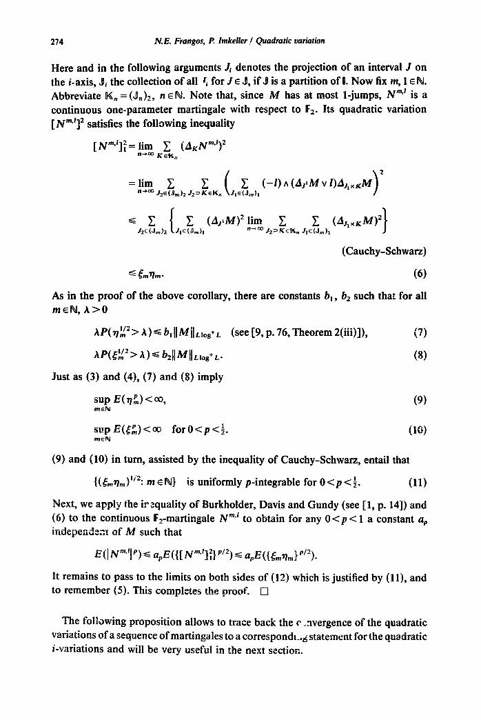
Here and in the following arguments Ji denotes the projection of an interval J on the i-axis, Jli the collection of all ri for J E JI, if JI is a partition of Il. Now fix m, 1 E N. Abbreviate IK, = (9,), , n E N. Note that, since M has at most l-jumps, NmV’ is a

continuous one-parameter martingale with respect to F2. Its quadratic variation [ IVm’12 satisfies the following ineyuality

(Cauchy-Schwarz)

s &n%n* (6)

As in the proof of the above corollary, there are constants bI, b2 such that for all mdV,h>O

Aw&!2> A)< hllMIILb,+L (see [9, p. 76, Theorem 2(iii)]), (7)

Just as (3) and (4), (7) and (8) imply

sup E(tg)<m forO<p<& m&4

(10)

(9) and (10) in turn, assisted by the inequality of Cauchy-Schwarz, entail that

{(&%n)‘i2: m E f+i} is uniformly p-integrable for 0 < p c $. (11)

Next, we apply the irsquality of Burkholder, Davis and Gundy (see [ 1, p. 143) and (6) to the continuous IF 2-martingale Nm*’ to obtain for any 0 < p < 1 a constant aP

ependezt of M such that

t remains to pass to the limits on both sides of (12) which is justified by (ll), and to remember (5). This compMes the proof. 0

position allows to trace back the c~_nvergence of the quadratic variations of a se nce of martingales to a corres ondl_.$ statement for the quadratic

e very useful in t

N.E. Frangos, P. Imkeller / Quadratic variation 275

osition 5. Let (M”),,N be a sequence of regular martingales in L log+ L

which have at most I-jumps. Assume that the sequences ([Mn]l)n,N and

(SUPt2~I [M”ltl,:~~)naN (suP,zEr [M*lfl,t~~~“EN

are bounded in Lp(s2,9,P) for O<p<& Then: if converges to 6 in L”(O, 9, P), ([ Mn]l)rieN converges to 0 in

Lp(Q 9, P) for Oap<$. A similar statement holds with respect to &jumps and quadratic 2-variations.

Proof. Proposition 4 and the inequality of Cauchy-Schwarx imply that the sequence ([Mn]:-[Mn]l),EN converges to 0 in Lp(Q SF, P) for Osp<$. To finish the proof, one only has to remark that

mfnl:-PIMnlf*,,~,, =N ryz1

and that, by Vitali’s convergence theorem, (suP~~~* [Mn]fl,r2j)nEN goes to 0 in kP(Q 9, P) as n-,00 for OspC$. Cl

.

2. The continuity of the quadratic variation

In this section, we will use the convergence results just obtained to derive the continuity properties of the quadratic variation [M] of a regular martingale M in L log+ L. Our principal method can be outlined as follows. Consider a sequence

(M”) nEN of “small” martingales approximating the “large” martingale M. Here “small” means ‘“5ounded” or, if this cannot be achieved, at least having better integrability properties. Due to the smallness of the M”, we possess information on the continuity properties of the quadratic variations [M”]. We make use of this information and apply Propositions ( 1.1) and ( 1.2) to deduce results on the continuity of [Ml.

If M has no O-jumps, we approximate it by its “trun&ons” M” = E(( -n) A (MI v n) 1%. ), n E N. Of course, M” may have O-jumps. But proposition (1.3) will enable us to see that the O-jump parts (M *)’ and M have orthogonal variation. This will imply that [M” - (M*)‘- M], + 0, so that proposition (1.1) is applicable.

In case for i = 1 or 2, M has at most i-jumps, it can be approximated by a sequence of bounded martingales which have the same continuity properties. Then, the corollary of Propositions (1.1) and (1.2) gives the desired result.

If M is continuous, we encounter the most difficult problem. As in the preceding case, we can approximate by a sequence ( ?jneN of bounded martingales with at most l-jumps (or at most &jumps). position (1.3) allows us to conclude that the

ave orthogonal variation for t E I. As a

consequence 0 osition (1 S) forces ition (1.1) is again r, could not be see

results for the remaining possible combinations of different kinds of jumps.

276 N.E. Frangos, P. Imkeller / Quadratic variation

For the defnitiun of the optional projections in the two parameter directions of bounded processes which appear in the proposition below, see for example [9, p. 491.

1. Let M be a regular martingale in L log+ L. Then the sequence of bounded martingales

M”= EC4 A ( 1 v n)lW, nw converges to M in L log+ L.

2. Let M be a reg :lar martinga!e in L log+ L which has at most l-jumps. For n E N, let N” be the continuous ane-parameter br,lartingale with respect to IF2 defined by stopping with respect to IF2 the continuous martingale M (1,. ) when its absolute value exceeds n for the first time, M n the optional projection of N” in direction I_ Then the bounded martingales M n, n E N, have at most 1 -jumps and converge to M in L log+ L. A similar statement holds with respect to the second parameter.

Proof. 1. The first part follows Y’rom the simple fact that

2. Let us turn to the less trivial second assertion. By [9, p. 621, Theorem 1, M n possesses at most l-jumps. Moreover, by definition, My + MI a.s. To complete the proof, we therefore have to show that the sequence ( IM~I lOg+lM yl)neN is uniformly integrab!e. To this end, according to Burkholder, Davis and Gundy [3, p. 2381, we may choose a convex function C$ : R+ + IR, such that

#1(0)=0, lim 4(t)/t=m and E(c#J(IM,I log+lM,I))<oo. t-00

Since the process ~(IM(J log+iM(,,.,I) is a submartingale with respect to IF*, we have

sup m#4lwl h+lM;o) n&J

,I log+lM$) c 00.

Now we only have to apply the lemma of de la Vallee-Poussin to obtain the desired uniform integrability. 0

has no O-jumps, then the O-jump parts he approximations n according to the first part of Proposition I, and

on. Similarly, if rW is continuous, the jump rding to tht . econd p

ogonal variation for a

N. E. Frangos, P. dmkeller / Quadratic wwiation 277

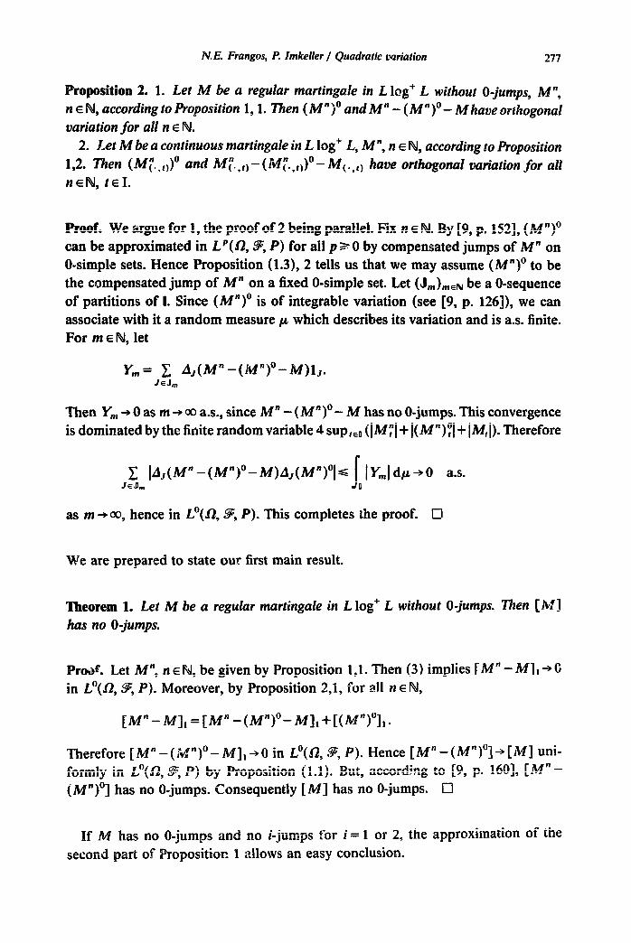
2. 1. Let be a regular martingale in L log+ L without O-jumps, n E N, according to Proposition 1,l. Then ( M n)” and M n - ( M n)” - M have orthogonal variation for ail n E N.

2. Let M be a continuous martingale in L log+ L, M”, n E N, according to Proposition 1,2. Ihen (M~.J” and M~.,I,-(M;.,I,)o-M~.,I, have orthogonal variation for all nEN, tE1.

Proof. We argue for I, the proof of 2 being parallel. Fix n E N. By [9, p. 1521, (M n)” can be approximated in Lp(O, 9, P) for all p a 0 by compensated jumps of M” on O-simple sets. Hence Proposition (1.3), 2 tells us that we may assume ( Mn)’ to be the compensated jump of M” on a fixed O-simple set. Let (Jm)mEN be a O-sequence of partitions of Il. Since ( Mn)’ is of integrable variation (see [9, p. 126]), we can associate with it a random measure p which describes its variation and is a.s. finite. For m E N, let

Ym = C AJ(Mn-(Mn)o-M)lJ. JEJ,

Then Y, + 0 as m + 00 a.s., since M n - ( Mn)’ - M has no O-jumps. This convergence isdominatedbythe~niterandomvariable4sup,,~(~M~~+~(M”)~~+~M,~).Therefore

c IA,(M”-(M~)o-M)A~(M~)oIS J IY,ldp+O ~P.s. Jd, II

as m + 00, hence in L”( J&S, P). This completes the proof. iX

We are prepared to state our first main result.

Theorem 1. Let M be a regular martingale in L log+ L without O-jumps. 7hen [M] has no O-jumps.

Let M”, n E N, be given by Proposition 1 ,l. Then (3) implies [ in L”(O, 9, P). Moreover, by Proposition 2,l, for all n E N,

Therefore [ n -(k?n)o- Ml*+0 in I?‘(J2, 9, P). Hence [Mn-(Mn)o]+[IM] uni- formly in L”(O, 9, P) by Proposition ( ). But, according to [9, p 1601, [M” - (M”)‘] has no O-jumps. Consequently [ 1 has no O-jumps. 0

-jumps and no i-jumps for i = I or 2, the approximation of the

opositior, 1 allows an easy conclusion.

278 IV. E. Frangos, I? lmkeller / Quadratic vwialion

Let M be a regular martingale in L log’ L which possesses at most B -jumps~ Then [M] possesses at most 1 jumps. An analogous result holds with respect to 2-jumps.

roof. Let “, n E N, be the approximating sequence of M according to Proposition

I1,2. Again by (3), [M” - M], + 0 in L*(R, ss P), and by Proposition (Ll), [M”] + [M] uniformly in L*(O, 9” P). But [M”] has at most l-jumps for all n E N, hence so does [Ml. q

We finally turn to continuous M. Before we present our final main result, however, a few remarks concerning the methods of proof are in order.

Given the procedure which yields Theorem 1, one is tempted to try the following method in order to deduce the continuity of [M] from the continuity of M. (a) Approximate M for example by the sequence (M’),EN of bounded martin- gales with at most l-jumps according to Proposition 1,2. (b) Show that the l-jump parts (M”)’ of M” and M” - (W)’ - A4 have orthogonal variation. (c) Conclude using Proposition (1.1). The difficult part of this seemingly natural procedure is to verify (b). To do this* it would be sufficient to see that ( W)’ and M have orthogonal variation But on the basis of the available Burkholder-Davis-Gundy type inequalities linking the quadratic variation of a two-parameter martingale to the supremum of its modulus, we were only able to prove orthogonality under more restrictive integrability assumptions than L log+ L. It seems conceivable to start with a Burkholder-Davis-Gundy type inequa!ity for the p-norms, 0 <p < 1, for con- tinuous martingales. Such an inequality, however, although probably true, has not yet been rigorously proved (see [9, p. 1651) and is out of the scope of this paper. This drawback forced us to take resort to a procedure which relates the convergence of quadratic variations to the convergence of quadratic i-variations, as given by Proposition (1.5). It only requires to verify an analogon of (b) for the one-parameter “sections” of M” and M Unfortunately, it produces another drawback: the question, whether inherits the remaining three combinations of different kinds of jumps

] seeps ta be inacicessible by the methods involved.

3. Let M be a continuous martingale in L log+ L. Then 1 M] is continuous.

n E IV, be given by Proposition 1,2. The proof of the corollary of and (1.2) shows that the sequences ([

I,,zJnEN converge to 0 in LP(R, S9 P) for 0

C ;.,f*r-M (-.,,,1:+~~~;..1,,~*1:~

for pz E N, tz E I, due to Proposition 2,2. Therefore

P4. E. Frangos, l? dmkeller / Quadratic variation

Next,

279

[M”], = [(M”)‘ll +[(M”)c]l, n EN (see [9, p. MO]).

This implies that together with ([Mn]l)neN also ([(MR)c]l)nEN, and (NM”)‘- mhd9 is bounded in Lp(C, 9, P) for 0~ p ~1. Since, however,

(M;l..r*j)O= (M”)t.*@ by definition for all n E N, proposition (1.5) can finally be applied to yield

[(M”)c-M],=[Mn-(M”)l-M]l+O inLP(O,@,P) forOsp<&

proposition (1.1) now gives [(M”)‘]+[M] uniformly in Lp(O, JF, P) for Osp<$.

Therefore [M] is continuous along with [(M”)‘], n E N, by [9, p. 158]. Cl

As an easy consequence of Theorem 3 and its proof we note the following approximation property.

Corollary. Let M be a continuous martingale in L log+ L. Then there exists a sequence

(MR),EN of continuous martingales which are q-integrable for all q 2 0 and which converge uniformly in 0 to M, in Lp(J2, 9, P) for all Osp< 1.

Proof. For n E N, kt M* be the continuous part of the nth approximation of M according to Proposition 1,2. Then M” is q-integrable for all q 3 0 by [9, p. 1541. The convergence assertion is then a co nsequence of the proof of Theorem 3 and of 19, p. 165, Theorem 21. I5

References

[l] J. Azgrna and M. Yor, En guise d’introduction, in: Temps Locaux, A&risque 52-53 (1973) (Sociiti mathematique de France) 3-22.

[2] D. Bakry, Sur la regularite des trajectoires des martingales B deux indices, Z. Wahrsch. VAT:. C&b. 50 (1979) 149-157.

[3] D.L. Burkholder, B. Davis and R.F. Gundy, Integral inequalities for convex functions of operators on martingales, Proc. Sixth Berkeley Symp. Math. Stats. Prob. 2 (1972) 223-240.

[4] D.L. Burkholder and R.F. Gundy, Extrapolation and interpolation of quasi-linear operators on martingales, Acta Math. 124 (1970) 249-304.

[S] R. Cairoli and J.B. Walsh, Stochastic integrals in the plane, Acta Math. 134 (1975) 111-183. [6] L. Chevalier, MartiGgaies continues & deux parametres, Bdi. SC. Math. (2j 136 (1982) 19-62. [7] N. Frangos and P. Im teller, Quadratic variation for a class of L log+ L-bounded two-parameter

martingales (1987), to nppear in Ann. Probab. [8] A.A. Gushchin, On the general theory of random fields on the plane, Russian Math. Surveys 37

(6) (1982) 55-80. [9] P. Imkeller, Habilitationaschrift (Univ. Miinchen, 1986).

[lo] A. Millet and L. Sucheston, On regularity of multi-parameter amarts and martingales, Z. Wahrsch. Verw. Geb. 56 (1981) 21-45.

[ 1 l] D. Nualart, On the quadratic variation of two-parameter continuous martingales, Ann. Probab. 12 (1984) 445-457.

[ 121 D. Nualart, Une formule d’It6 pour les martingales continues a deux indices et quelques applications, Ann. Inst. Henri Poincare 20 (1984) 251-275.