Stochastic Neuroscience

Bard Ermentrout

Dept of MathUniversity of Pgh

Pgh PA

CLARENDON PRESS . OXFORD

2008

1

NOISY OSCILLATORS

Synchronous oscillations occur throughout the central nervous system. Record-ings of population activity such as the electorencephalogram (EEG) and localfield potential (LFP) often show a strong peak in the power spectrum in certainfrequencies. This synchronous activity is sometimes observed across multiplerecording sites and over distant brain areas. While local circuitry in the cortexis ideal for the production of local rhythms, the mechanisms for synchronizationacross different regions are more complex. Furthermore, the rhythms observed inreal biological networks are not perfect oscillations. Instead, correlations betweencells are often weak and the width of peaks in the power spectrum can also bequite broad. There are many reasons for this imperfect synchronization. Amongthem are heterogenity in properties of individual neurons, heterogenities in theconnectivity between cells and their inputs, and finally, intrinsic noise (due, e.g.to channel fluctuations as well as the aforementioned heterogenities). The goal ofthis chapter is to analyze the role of noise in synchronizing and desynchronizingcoupled oscillators using a particularly simple class of model oscillators.

There is a long history of the study of noise in oscillators, going back to thework of Stratonovich (35; 36) where the interest was on how noise could disruptoscillatory radio circuits. Our focus in this chapter concerns how noise affectsneural oscillators, both in isolation and when coupled to each other. Furthermore,we will mainly consider the behavior when the noise and coupling are smalland the oscillators are nearly identical. This allows one to significantly reducethe dimensionality of the problem and treat each oscillator as a single variablecoding its phase. In other chapters of this book (notably Longtin), the effects oflarger noise will be studied on systems which may not even intrinsically oscillate(coherence resonance).

The overall organization of this chapter is as follows. First we consider thegeneral question of perturbed oscillators and introduce the phase resetting curve.We then look at how correlated noise can serve as a synchronizing signal foruncoupled oscillators. We study how noise can desynchronize coupled oscillators.We first study a pair and then a large network of globally coupled oscillators usingpopulation density methods.

1.1 The phase resetting curve & weak perturbations.

1.1.1 Preliminaries.

Many authors (particularly in physics) define an oscillator to be any dynami-cal system which makes repeated (although not necessarily predictable) transits

2 Noisy oscillators

through some local region in phase space. For example, chaotic systems are oftencalled oscillators. In this chapter, we confine our attention to systems in whichthere is an underlying attracting limit cycle, X0(t) such that X0(t+T ) = X0(t).We suppose that this satisfies an ordinary differential equation:

dX

dt= F (X(t)) (1.1)

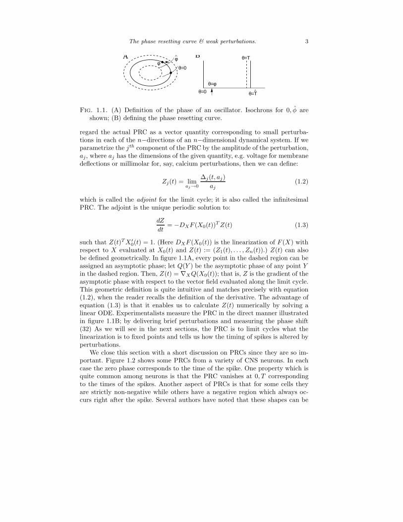
All autonomously generated limit cycles have an arbitrary phase associated withthem. Thus, let us define the phase of the limit cycle to be t modulo T , witht = 0 defined as some identifiable point on the cycle. Since our main examplescome from neuroscience, the 0 phase, is often defined as the time of the spike.Thus a rhythmically firing neuron produces spikes at multiples of T . Now, sup-pose that we add to this a possibly noisy, time dependent perturbation, which is“weak” in the sense that it does not destroy the overall shape of the limit cycle.Formally, the limit cycle attractor is a closed orbit in phase space and there isa local tubular neighborhood of the cycle in which all points of this neighbor-hood are attracted to the limit cycle with a well-defined asymptotic phase. Theperturbation should be small enough so as not to leave this neighborhood. Inpractice, it can be quite large. Since each point in the neighborhood has a well-defined phase, there are curves called isochrons which parametrize the phase ofevery point on the limit cycle (20; 22; 43; 17). Figure 1.1A shows a neighborhood(dashed ellipses) around a limit cycle with the zero phase, θ = 0 defined to bethe maximum in the horizontal direction. Phase increases at a constant rate inthe counterclockwise direction. The curve passing through θ = 0 is the 0-phaseisochron. Any points on this curve will asymptotically approach the unshiftedoscillator. Consider a brief (instantaneous) stimulus in the horizontal directionoccurring at phase φ. The perturbation will cause the dynamics to leave thelimit cycle, but, if it is sufficiently small, it will remain in a neighborhood wherethe asymptotic phase is defined. Figure 1.1A shows that the perturbation movesthe limit cycle from its current phase, φ to a new phase, φ. The mapping fromφ to φ is called the phase transition curve (PTC). The net change in phase is

the phase resetting curve (PRC), ∆(φ) := φ− φ. Note that in this example, thechange in phase is negative and the time of the next maximum will be delayed.An alternate way to look at the PRC is through the spike (or event) time. Fig-ure 1.1B shows how the PRC is constructed in this manner. The perturbation isgiven at phase φ producing the next spike/event at a time T . The PRC is then,∆(φ) := T − T . As above, in this example, the next spike is delayed so PRC atthis value of phase is negative. We should remark that the PRC is often definedin terms of a phase between 0 and 1 or 0 and 2π. In this case, one only needsto divide by the period T and multiply by 2π. We prefer to work using the realtime of spike, but it doesn’t matter.

In the above geometric example, the perturbation was a horizontal kick;of course, there could also be a vertical kick which would give a PRC in they−direction. If the kicks are small, then the effects add linearly, so that we can

The phase resetting curve & weak perturbations. 3

φ^

θ=Τ

θ=0φ

θ=0

θ=Τ

θ=φ

A B

Fig. 1.1. (A) Definition of the phase of an oscillator. Isochrons for 0, φ areshown; (B) defining the phase resetting curve.

regard the actual PRC as a vector quantity corresponding to small perturba-tions in each of the n−directions of an n−dimensional dynamical system. If weparametrize the jth component of the PRC by the amplitude of the perturbation,aj , where aj has the dimensions of the given quantity, e.g. voltage for membranedeflections or millimolar for, say, calcium perturbations, then we can define:

Zj(t) = limaj→0

∆j(t, aj)

aj

(1.2)

which is called the adjoint for the limit cycle; it is also called the infinitesimalPRC. The adjoint is the unique periodic solution to:

dZ

dt= −DXF (X0(t))

TZ(t) (1.3)

such that Z(t)TX ′

0(t) = 1. (Here DXF (X0(t)) is the linearization of F (X) withrespect to X evaluated at X0(t) and Z(t) := (Z1(t), . . . , Zn(t)).) Z(t) can alsobe defined geometrically. In figure 1.1A, every point in the dashed region can beassigned an asymptotic phase; let Q(Y ) be the asymptotic phase of any point Yin the dashed region. Then, Z(t) = ∇XQ(X0(t)); that is, Z is the gradient of theasymptotic phase with respect to the vector field evaluated along the limit cycle.This geometric definition is quite intuitive and matches precisely with equation(1.2), when the reader recalls the definition of the derivative. The advantage ofequation (1.3) is that it enables us to calculate Z(t) numerically by solving alinear ODE. Experimentalists measure the PRC in the direct manner illustratedin figure 1.1B; by delivering brief perturbations and measuring the phase shift(32) As we will see in the next sections, the PRC is to limit cycles what thelinearization is to fixed points and tells us how the timing of spikes is altered byperturbations.

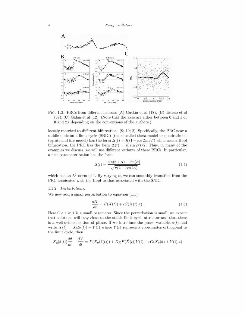
We close this section with a short discussion on PRCs since they are so im-portant. Figure 1.2 shows some PRCs from a variety of CNS neurons. In eachcase the zero phase corresponds to the time of the spike. One property which isquite common among neurons is that the PRC vanishes at 0, T correspondingto the times of the spikes. Another aspect of PRCs is that for some cells theyare strictly non-negative while others have a negative region which always oc-curs right after the spike. Several authors have noted that these shapes can be

4 Noisy oscillators

A

B C

Fig. 1.2. PRCs from different neurons (A) Gutkin et al (18), (B) Tateno et al(39); (C) Galan et al (12). (Note that the axes are either between 0 and 1 or0 and 2π depending on the conventions of the authors.)

loosely matched to different bifurcations (9; 19; 2). Specifically, the PRC near asaddle-node on a limit cycle (SNIC) (the so-called theta model or quadratic in-tegrate and fire model) has the form ∆(t) = K(1− cos2πt/T ) while near a Hopfbifurcation, the PRC has the form ∆(t) = K sin 2πt/T. Thus, in many of theexamples we discuss, we will use different variants of these PRCs. In particular,a nice parameterization has the form

∆(t) =sin(t+ α) − sin(α)√

π(2 − cos 2α)(1.4)

which has an L2 norm of 1. By varying α, we can smoothly transition from thePRC assoicated with the Hopf to that associated with the SNIC.

1.1.2 Perturbations.

We now add a small perturbation to equation (1.1):

dX

dt= F (X(t)) + ǫG(X(t), t). (1.5)

Here 0 < ǫ≪ 1 is a small parameter. Since the perturbation is small, we expectthat solutions will stay close to the stable limit cycle attractor and thus thereis a well-defined notion of phase. If we introduce the phase variable, θ(t) andwrite X(t) = X0(θ(t)) + Y (t) where Y (t) represents coordinates orthogonal tothe limit cycle, then

X ′

0(θ(t))dθ

dt+dY

dt= F (X0(θ(t))) +DXF (X(t))Y (t) + ǫG(X0(θ) + Y (t), t)

The phase resetting curve & weak perturbations. 5

where X is close to X0 and X. If we multiply this equation by Z(t)T , we obtain

dθ

dt= 1 + Z(t)T [−Y ′(t) +DXF (X(t))Y (t)] + ǫZ(t)TG(X0(t) + Y (t), t).

(Note that we have used the fact that Z(t)TX0(t)′ = 1.) This is an exact equation

for the evolution of the phase; it is not an approximation. However, it still involvesY (t) and X(t) which are unknown. Note also, that we have not used the smallnessof ǫ except to assume that the perturbation remains in a region for which phase isdefined. If ǫ is small, Y (t), too, will be of order ǫ and X will be close toX0.We willexploit this to obtain an approximate equation for the phase. The linear operator,L(t)Y := −Y ′ + DXF (X0(t))Y has a one dimensional nullspace spanned byX ′

0(t) and its adjoint (under the usual inner product for periodic systems) hasa nullspace spanned by Z(t). Thus, with the approximation X ≈ X ≈ X0, weobtain the self-contained phase model:

dθ

dt= 1 + ǫZ(θ)TG(X0(θ), t). (1.6)

This is the main equation of this chapter and we will use it to analyze the effectsof noise and coupling of oscillators. We note that in the case of neuronal models,the perturbations are typically only through the somatic membrane potential sothat the all but one of the components ofG are zero and we can more convenientlywrite

θ′ = 1 + ǫ∆(θ)g(θ, t). (1.7)

Remarks.

1. If the perturbation is a white noise, then we have to be a bit more carefuland make sure we interpret this process correctly since the normal changesof variables that we take need to be adjusted in accordance to the rules ofstochastic calculus (33). Thus, if the perturbation is white noise, then thecorrect version of (1.7) is (40):

dθ = [1 + ǫ2∆′(θ)∆(θ)/2]dt + ǫ∆(θ)dW (t) (1.8)

where dW (t) is a zero mean unit variance Gaussian.

2. The perturbations incorporated in G in equation (1.5) could be the effectsof other oscillators to which our example oscillator is coupled via, e.g.,synapses or gap junctions. We will consider this in later sections.

1.1.3 Statistics.

In this section, we derive equations for the mean and variance of the interspikeinterval for noisy oscillators as well as show that the variance of the phase-resetting curve is phase-dependent. We first consider the nonwhite case for whichthe perturbation is zero mean:

θ′ = 1 + ǫ∆(θ)ξ(t).

6 Noisy oscillators

Here ξ(t) is the “noise.” We look for a solution of the form: θ(t) = t + ǫθ1(t) +ǫ2θ2(t) + . . . and obtain:

θ1(t) =

∫ t

0

∆(s)ξ(s) ds.

Similarly,

θ2(t) =

∫ t

0

∫ s

0

∆′(s)∆(s′)ξ(s)ξ(s′) ds ds′.

The unperturbed period is T , so that we want to find the value of t∗ such thatθ(t∗) = T. Thus, we expect t∗ = T + ǫτ1 + ǫ2τ2 + . . ., which results in

τ1 = −∫ T

0

∆(s)ξ(s) ds

and

τ2 = −∆(T )ξ(T )τ1 −∫ T

0

∫ s

0

∆′(s)∆(s′)ξ(s)ξ(s′) ds ds′.

Let C(t) := 〈ξ(0)ξ(t)〉 be the autocorrelation function for the noisy perturbation(which we assume is stationary with zero mean). We see that the expected periodof the oscillation is just

T = T + ǫ〈τ1〉 + ǫ2〈τ2〉.To order ǫ, there is no effect of the signal since the mean of τ1 is zero. However,there are second order effects:

〈τ2〉 = ∆(T )

∫ T

0

∆(s)C(s− T ) ds−∫ T

0

∫ s

0

∆′(s)∆(s′)C(s− s′) ds ds′. (1.9)

The variance (to order ǫ2) is

var = ǫ2〈τ21 〉 = ǫ2

∫ T

0

∫ T

0

∆(s)∆(s′)C(s− s′) ds ds′. (1.10)

For a simple low-pass filtered white noise process (Ornstein-Uhlenbeck), C(t) =exp(−|t|/τ)/2 so that these integrals can be readily evaluated for simple PRCssuch as (1.4).

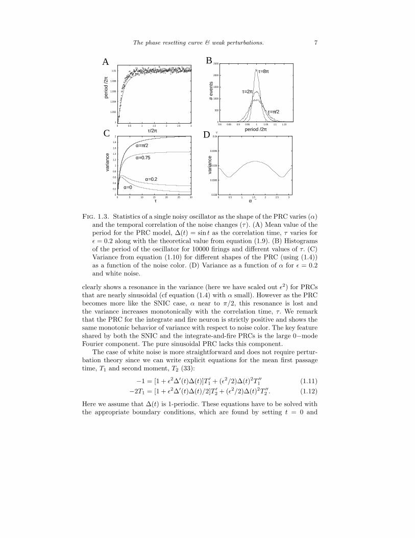
Figure 1.3 shows some numerical as well as analytical results on the effects ofthe noise color on the statistics of weakly perturbed oscillators. As noted above,there is a weak effect on the mean period of the oscillator for colored noiseas seen in figure 1.3A that is well-accounted for by the theoretical expressionin equation (1.9). For a purely sinusoidal PRC, there is a “resonance” in thevariance as a function of the noise color. That is, the variance has a maximumwhen the temporal correlations are proportional to the period of the oscillatoras seen by the width of the histograms in figure 1.3B. Using equation (1.10),we can make this more explicit by evaluating the double integrals. Figure 1.3C

The phase resetting curve & weak perturbations. 7

1

1.002

1.004

1.006

1.008

1.01

0 0.5 1 1.5 2 2.5 3

0

500

1000

1500

2000

2500

0.8 0.85 0.9 0.95 1 1.05 1.1 1.15

0

0.2

0.4

0.6

0.8

1

1.2

1.4

1.6

1.8

2

0 5 10 15 20 25 300.038

0.0385

0.039

0.0395

0.04

V

0 0.5 1 1.5 2 2.5 3al

period /2π

perio

d/2

π

τ/2π

Aτ=8π

τ=2π

τ=π/2

# ev

ents

B

α=0.75

α=π/2

α=0.2

α=0

τ

varia

nce

C

varia

nce

α

D

Fig. 1.3. Statistics of a single noisy oscillator as the shape of the PRC varies (α)and the temporal correlation of the noise changes (τ). (A) Mean value of theperiod for the PRC model, ∆(t) = sin t as the correlation time, τ varies forǫ = 0.2 along with the theoretical value from equation (1.9). (B) Histogramsof the period of the oscillator for 10000 firings and different values of τ. (C)Variance from equation (1.10) for different shapes of the PRC (using (1.4))as a function of the noise color. (D) Variance as a function of α for ǫ = 0.2and white noise.

clearly shows a resonance in the variance (here we have scaled out ǫ2) for PRCsthat are nearly sinusoidal (cf equation (1.4) with α small). However as the PRCbecomes more like the SNIC case, α near to π/2, this resonance is lost andthe variance increases monotonically with the correlation time, τ. We remarkthat the PRC for the integrate and fire neuron is strictly positive and shows thesame monotonic behavior of variance with respect to noise color. The key featureshared by both the SNIC and the integrate-and-fire PRCs is the large 0−modeFourier component. The pure sinusoidal PRC lacks this component.

The case of white noise is more straightforward and does not require pertur-bation theory since we can write explicit equations for the mean first passagetime, T1 and second moment, T2 (33):

−1 = [1 + ǫ2∆′(t)∆(t)]T ′

1 + (ǫ2/2)∆(t)2T ′′

1 (1.11)

−2T1 = [1 + ǫ2∆′(t)∆(t)/2]T ′

2 + (ǫ2/2)∆(t)2T ′′

2 . (1.12)

Here we assume that ∆(t) is 1-periodic. These equations have to be solved withthe appropriate boundary conditions, which are found by setting t = 0 and

8 Noisy oscillators

exploiting the fact that ∆(0) = 0, thus, T ′

1(0) = −1, T1(1) = 0 and T ′

2(0) =−2T1(0), T2(1) = 0. The mean period is T1(0) and the variance is T2(0)−T1(0)2.Explicit expressions for these quantities could be found (?), but they involveintegrals that are not readily evaluated. Instead, we can solve the boundary valueproblem by shooting or some other technique and compute how the variancedepends on shape of the PRC. Figure 1.3D shows this dependence for ǫ = 0.2.The variance remains less than would be the case for a constant PRC (var=ǫ2 =0.04) and is maximal when α = π/2 corresponding to the SNIC bifurcation.

As a last look at statistics, we can study the effect of noise on the actualcalculation of the phase resetting curve. In particular, we consider the followingsimple model:

dθ

dt= 1 + [ǫξ(t) + βδ(t− φ)]∆(θ) (1.13)

which represents the noise ξ(t) along with a Dirac delta function perturbationfor the PRC. Here φ is the time of the perturbation and lies between 0 and T ,the period. The net gain in phase given θ(0) = 0 is found by evaluating θ(T ).In absence of any stimuli (noise or experimental perturbations), θ(T ) = T. Fora completely noise-free system, θ(T ) = T + β∆(φ) so that the gain (or loss) inphase is just θ(T )−T = β∆(φ) as it should be; the PRC of the noise free systemshould be proportional to ∆(τ). With noise, θ(T ) is a random variable. Usingperturbation theory, it is possible to show that the mean value of θ(T ) is thesame as the noise-free case, but that the variance is phase-dependent. In fact,we have shown (unpublished work) that for white noise:

var(φ) = ǫ2

(

[1 + β∆′(φ)]2∫ φ

0

∆2(s) ds+

∫ T

φ

∆2(s+ β∆(φ)) ds

)

. (1.14)

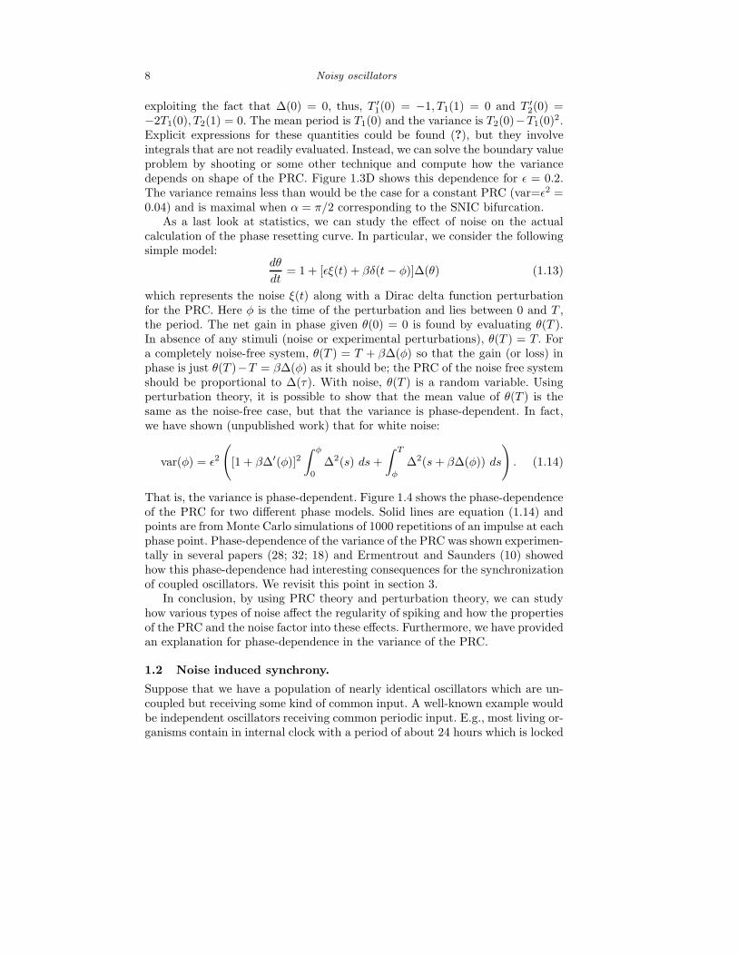
That is, the variance is phase-dependent. Figure 1.4 shows the phase-dependenceof the PRC for two different phase models. Solid lines are equation (1.14) andpoints are from Monte Carlo simulations of 1000 repetitions of an impulse at eachphase point. Phase-dependence of the variance of the PRC was shown experimen-tally in several papers (28; 32; 18) and Ermentrout and Saunders (10) showedhow this phase-dependence had interesting consequences for the synchronizationof coupled oscillators. We revisit this point in section 3.

In conclusion, by using PRC theory and perturbation theory, we can studyhow various types of noise affect the regularity of spiking and how the propertiesof the PRC and the noise factor into these effects. Furthermore, we have providedan explanation for phase-dependence in the variance of the PRC.

1.2 Noise induced synchrony.

Suppose that we have a population of nearly identical oscillators which are un-coupled but receiving some kind of common input. A well-known example wouldbe independent oscillators receiving common periodic input. E.g., most living or-ganisms contain in internal clock with a period of about 24 hours which is locked

Noise induced synchrony. 9

0.12

0.13

0.14

0.15

0.16

0.17

0.18

0.19

0.2

0.21

0 0.2 0.4 0.6 0.80.2

0.22

0.24

0.26

0.28

0.3

0.32

0.34

0 0.2 0.4 0.6 0.8 1

A B

S.D

.

phasephase

S.D

.

Fig. 1.4. Standard deviation (square root of the variance) of the PRC for (A)∆(t) = sin 2πt and (B) ∆(t) = 1 − cos 2πt. Here ǫ = 0.1 and β = 1/(8π).

to the light-dark cycle as the earth circles the sun. Thus, even though these os-cillators are not directly coupled, the periodic drive they receive is sufficient forthem to partially synchronize. Of course, the frequency of the periodic drivemust match that of the individual oscillators in order for this to work. What issurprising is that the common signal received by the uncoupled oscillators neednot be periodic.

Pikovsky and his collaborators were among the first to describe models andtheory for the synchronization of dynamical systems to common noisy input (16;?; 31). These authors look not only at oscillators but also at chaotic systems andother systems with complex dynamics. They have also shown that for strongnoise, synchrony is disrupted. Jensen (21) studied an abstract phase model foroscillators receiving a common signal and Ritt (34) analyzed synchronization ofa specific model (the theta model) to white noise. In this section, we will usephase response curves once again to explore synchrony when they are uncoupledbut receive a common noisy input. The methods described here are close to thoseof Teramae and Tanaka (40).

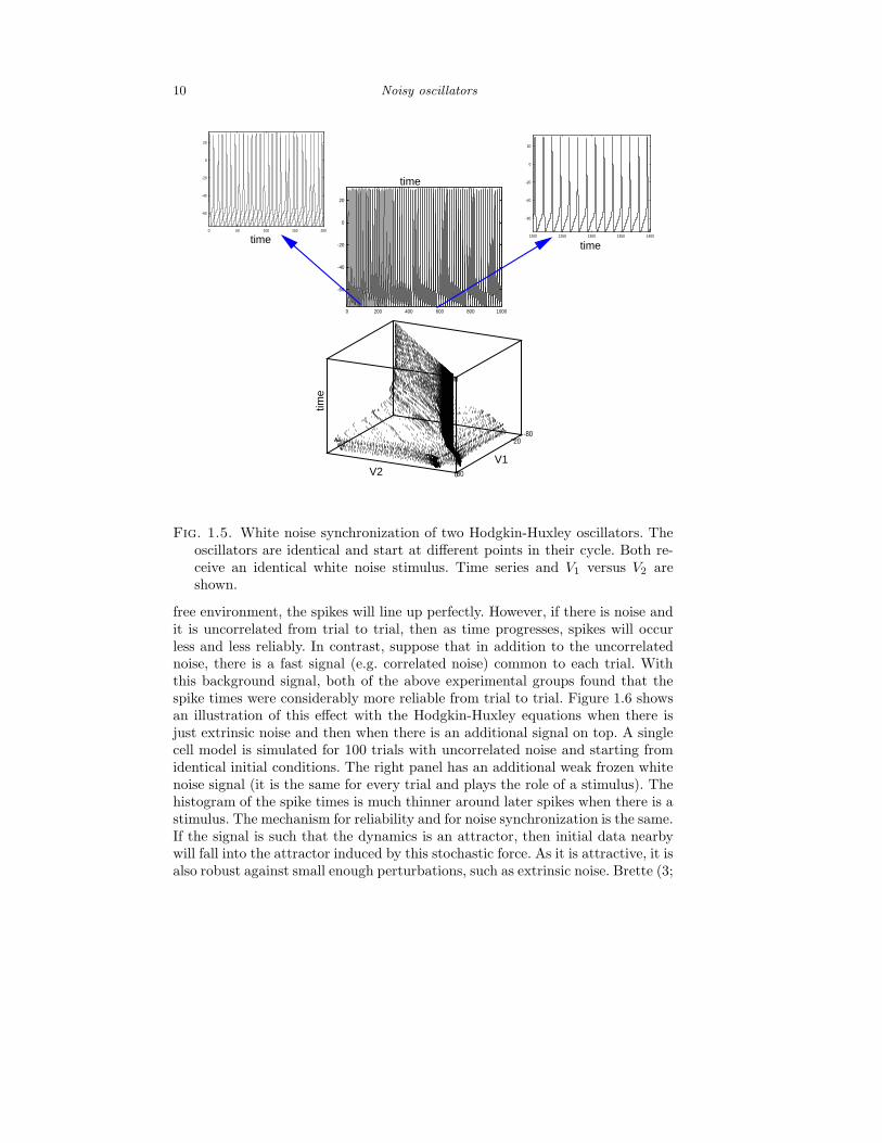
Figure 1.5 shows an example of a synchronization due to a common input fortwo Hodgkin-Huxley oscillators. Voltages are plotted against time in the upperplots and against each other in the three-dimensional plot below. The cells areidentical, uncoupled, and start with a phase difference of half a cycle. Theyare driven by weak white noise and after several cycles, the phase-differencedisappears and the oscillators are completely synchronized. This phenomena isnot restricted to neural models; Galan et al (13) demonstrated that filtered whitenoise stimuli could synchronize mitral cells in the olfactory bulb. This mechanismis called the Moran effect in ecology (8) and has also been suggested as a meansto synchronize intracellular signalling oscillations (44). The goal in this sectionis to use phase models to study how noise can synchronize uncoupled oscillators.The mechanism for this type of synchronization is closely related to the issue ofspike time reliability as first discussed by (5) and popularized by (45) To see theconnection, suppose that we apply a constant current to a neuron to induce itto fire repetitively and mark the times of the spike. We repeat this experimentmany times and create a histogram of the spike times. In a completely noise-

10 Noisy oscillators

-80

20-80

20

0

2000

-60

-40

-20

0

20

0 200 400 600 800 1000

-60

-40

-20

0

20

0 50 100 150 200

-60

-40

-20

0

20

1200 1250 1300 1350 1400

timetime

time

time

V2V1

Fig. 1.5. White noise synchronization of two Hodgkin-Huxley oscillators. Theoscillators are identical and start at different points in their cycle. Both re-ceive an identical white noise stimulus. Time series and V1 versus V2 areshown.

free environment, the spikes will line up perfectly. However, if there is noise andit is uncorrelated from trial to trial, then as time progresses, spikes will occurless and less reliably. In contrast, suppose that in addition to the uncorrelatednoise, there is a fast signal (e.g. correlated noise) common to each trial. Withthis background signal, both of the above experimental groups found that thespike times were considerably more reliable from trial to trial. Figure 1.6 showsan illustration of this effect with the Hodgkin-Huxley equations when there isjust extrinsic noise and then when there is an additional signal on top. A singlecell model is simulated for 100 trials with uncorrelated noise and starting fromidentical initial conditions. The right panel has an additional weak frozen whitenoise signal (it is the same for every trial and plays the role of a stimulus). Thehistogram of the spike times is much thinner around later spikes when there is astimulus. The mechanism for reliability and for noise synchronization is the same.If the signal is such that the dynamics is an attractor, then initial data nearbywill fall into the attractor induced by this stochastic force. As it is attractive, it isalso robust against small enough perturbations, such as extrinsic noise. Brette (3;

Noise induced synchrony. 11

0 50 100 150 200 250 300 350 400 450 500

0

0 100 200 300 400 500

time (msec)

no stimulus stimulus

time (msec)

Fig. 1.6. Reliability in the Hodgkin-Huxley model. 100 trials of a constantcurrent injection with uncorrelated noise (amplitude 1) with no stimulus andthen with a common white noise stimulus (amplitude=15). Spike times andhistograms (below) are shown.

4) analyzed these spike-time attractors for the integrate-and-fire model; Troyer(41) also analyzes these attractors in a context similar to that described here.We will formalize the notion of stability in the next several pages and introducethe so-called Lyapunov exponent.

1.2.1 White noise.

Pikovsky (30) was among the first to analyze synchronization to noise when hestudied Poisson inputs. More recently, this work has been extended to white noiseand to more general synchronization issues. We will follow Teramae and Tanakafor the white noise case and sketch the analysis for the Poisson case as well. Westart with a single oscillator driven by white noise and reduced to a phase model.As our motive is to study neuronal oscillations, we will confine ourselves to thecase when white noise appears only in the voltage equation. For any regularperturbations, equation (1.6) is valid, however, when the noise is white, we haveto be careful and make the correct change of variables using the Ito stochasticcalculus, so that we start with equation (1.8). Solutions to this equation have aninvariant density found by solving the steady state Fokker-Planck equation:

0 = [(1 +D∆′(x)∆(x))ρ(x) +D(∆(x)2ρ(x))′]′

where D = ǫ2/2 and ρ(x) is the invariant density; that is the probability that

θ ∈ [a, b] is∫ b

aρ(x)dx. This differential equation must be solved subject to ρ(x)

is periodic and∫ T

0ρ(x) dx = 1, the normalization. Solutions can be found by

integrating or, since D is small, using perturbation theory. For our purposes,the invariant density is close to being uniform when D is small, so that we willapproximate ρ(x) by 1/T. Consider two oscillators driven with the same whitenoise signal:

dθ1 = [1 +D∆′(θ1)∆(θ1)]dt+ ǫ∆(θ1)dW (1.15)

12 Noisy oscillators

dθ′2 = [1 +D∆′(θ2)∆(θ2)]dt+ ǫ∆(θ2)dW.

We are interested in whether or not they will synchronize. That is, we would liketo assess the stability of the state θ2 = θ1. We let θ2 − θ1 = y(t) and thus studythe variational equation which has the form

dy = [D∆′(θ)∆(θ)]′ydt+ ǫ∆′(θ)ydW.

Here θ(t) satisfies equation (1.8). This is a linear SDE in y(t) and we would liketo solve it. Let z(t) = log y(t) be a change of variables. Then appealing to Ito’sformula, we find that

dz = D[(∆′(θ)∆(θ))′ − ∆′(θ)2]dt+ ǫ∆′(θ)dW.

This is now a standard stochastic equation and we can integrate it to obtain themean drift in z(t) :

λ := D limt→∞

∫ t

0

[(∆′(θ(s))∆(θ(s)))′ − ∆′(θ(s))2] ds.

This is the mean rate of growth of y(t) so that if λ < 0, then y(t) will decay andsynchrony will be stable. The quantity, λ is called the Lyapunov exponent andsince our system is ergodic, we obtain a simple expression:

λ = D

∫ T

0

[(∆′(x)∆(x))′ − ∆′(x)2]ρ(x) dx.

Using the approximation that ρ(x) ≈ 1/T and the periodicity of ∆(x), we find

λ = −D 1

T

∫ T

0

∆′(x)2 dx. (1.16)

This is the main result on the stability of synchrony with identical white noisestimuli. It was derived by Teramae and Tanaka (40) for the white noise case.What it tells us is that the details of the oscillator are irrelevant, the Lyapunovexponent is always negative for weakly forced oscillators.

As we begun this section out by discussing reliability, it is interesting to relatereliability to the magnitude of the Lyapunov exponent. In (14) we show that thereliability (measured as the ratio of the cross correlation of the output and theauto-correlation) is

R =|λ|

|λ| + c

where c ≥ 0 is the magnitude of the extrinsic noise which is uncorrelated betweenthe neurons. Note that if c = 0, then reliability is 1, which is perfect. For small λ,reliability decreases which is why we generally want to maximize the magnitudeof λ.

Noise induced synchrony. 13

1.2.2 Poisson and colored noise.

Pikovsky (30) and others (26) have also studied the case of Poisson inputs. Letθn denote the phase of an oscillator right before the nth impulse where the trainof impulses obeys some type of distribution. Assume each has an amplitude ǫand we obatin a model for the phase:

θn+1 = θn + In + ǫ∆(θn) mod T

where In is the time between impulses. As with the white noise case, it is pos-sible to write an equation for the invariant density. Let Q(I) denote the densityfunction for the intervals, In modulo the period, T. (Thus, the support of Q isthe interval [0, T ).) Then the invariant density for the phase θ, ρ(x) satisfies thelinear integral equation:

ρ(x) =

∫ T

0

Q[x− y − ǫ∆(y)]ρ(y) dy.

(See (23; 10; 27).) In this case, the Lyapunov exponent satisfies:

λP =

∫ T

0

log[1 + ǫ∆′(x)]ρ(x) dx.

For ǫ small, ρ(x) is nearly uniform and expanding in ǫ, we find the same expres-sion for λP as for the white noise case.

We can use equation (1.6) for colored noise in order to study the stability ofsynchrony. As in the rest of this section, the single oscillator satisfies

dθ

dt= 1 + ǫ∆(θ)ξ(t)

where ξ(t) is a general process. The variational equation satisfies

dy

dt= ǫ∆′(θ(t))ξ(t)y(t)

and the Lyapunov exponent is

λξ = ǫ limt→∞

1

t

∫ t

0

∆′(θ(s))ξ(s) ds.

Using perturbation theory, as above, θ(t) = t+ǫ∫ t

0∆(s)ξ(s) ds can be substituted

into the equation for λξ and obtain:

λξ = limt→∞

1

t

∫ t

0

∆′′(s)

∫ s

0

∆(s′)C(s− s′) ds′ ds (1.17)

where C(t) is once again the autocorrelation of the common noise. For low passfiltered noise and ∆(t) as in equation (1.4), we obtain:

λξ = −ǫ2 1

2π(2 − cos 2α)

τ

1 + τ2.

This shows that the Lyapunov exponent shows “resonance” with respect to thePRC shape. For this model, the minimum occurs when τ = 1. Figure 1.7A shows

14 Noisy oscillators

A B

Fig. 1.7. Reliability of real and model neurons (from (14)). (A) Reliability isa nonmonotonic function of the correlation time of the signal for both real(mitral and pyramidal neurons) and model neurons. (B) Reliability increasesmonotonically with signal amplitude.

an experimental verification of the dependence of reliability on the correlationtime of the signal, ξ(t). Since reliability is a monotonic function of the Liapunovexponent, this shows that the above calculations hold in realistic settings forboth real and model neurons. Reliability is also a monotonic function of thenoise amplitude for a given correlation time as can be seen from 1.7B.

1.2.3 Heterogeneity and extrinsic noise.

In figure 1.5, we showed that perfectly correlated noise produces a perfectlysynchronized state. How does this change in the presence of heterogenities orin uncorrelated noise. Nakao et al (27) consider the white noise problem whenthere is a mixture of identical and uncorrelated noise. We can generalize thatslightly to study the case when there is additionally heterogeneity in the naturalfrequencies of the oscillators. The generalization of equation (1.15) is

dθ1 = [1 − µ/2 + (ǫ2/2)∆′(θ1)∆(θ1)]dt+ ǫ∆(θ1)(√qdW +

√

1 − qdW1)

dθ′2 = [1 + µ/2 + (ǫ2/2)∆′(θ2)∆(θ2)]dt+ ǫ∆(θ2)(√qdW +

√

1 − qdW2).

where µ is the difference in natural frequency and q is the fraction of sharednoise. When q = 1, µ = 0, then the oscillators receive identical noise and have nointrinsic differences, in short, equation (1.15). Nakao et al develop an equationfor the probability density function for the phase-difference, θ2 − θ1 for small ǫwhen µ = 0. If we rescale µ = ǫ2µ, then we can generalize their result and obtainthe following equation for the density of the phase differences:

[(1 − ch(x)

h(0))ρ(x)]′ = K + µρ(x) (1.18)

Noise induced synchrony. 15

0

1

2

3

4

5

6

7

0 0.05 0.1 0.15 0.2 0.25 0.3 0.35 0.4 0.45 0.50

0.5

1

1.5

2

2.5

3

3.5

4

4.5

0 0.2 0.4 0.6 0.8 1ρ(

x)

ρ(x)

x x

0.1

0.95

0.9

0.75

0.5

0

2

5

−2

−5

0

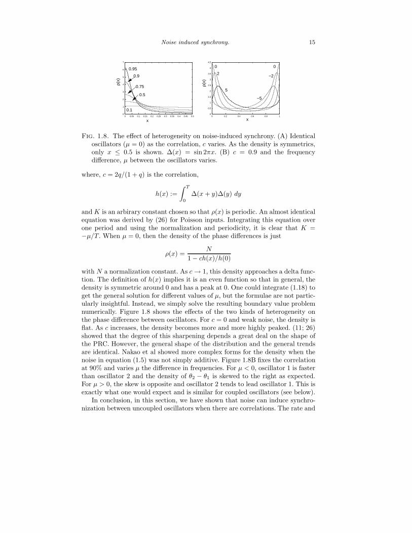
Fig. 1.8. The effect of heterogeneity on noise-induced synchrony. (A) Identicaloscillators (µ = 0) as the correlation, c varies. As the density is symmetrics,only x ≤ 0.5 is shown. ∆(x) = sin 2πx. (B) c = 0.9 and the frequencydifference, µ between the oscillators varies.

where, c = 2q/(1 + q) is the correlation,

h(x) :=

∫ T

0

∆(x + y)∆(y) dy

and K is an arbirary constant chosen so that ρ(x) is periodic. An almost identicalequation was derived by (26) for Poisson inputs. Integrating this equation overone period and using the normalization and periodicity, it is clear that K =−µ/T. When µ = 0, then the density of the phase differences is just

ρ(x) =N

1 − ch(x)/h(0)

with N a normalization constant. As c→ 1, this density approaches a delta func-tion. The definition of h(x) implies it is an even function so that in general, thedensity is symmetric around 0 and has a peak at 0. One could integrate (1.18) toget the general solution for different values of µ, but the formulae are not partic-ularly insightful. Instead, we simply solve the resulting boundary value problemnumerically. Figure 1.8 shows the effects of the two kinds of heterogeneity onthe phase difference between oscillators. For c = 0 and weak noise, the density isflat. As c increases, the density becomes more and more highly peaked. (11; 26)showed that the degree of this sharpening depends a great deal on the shape ofthe PRC. However, the general shape of the distribution and the general trendsare identical. Nakao et al showed more complex forms for the density when thenoise in equation (1.5) was not simply additive. Figure 1.8B fixes the correlationat 90% and varies µ the difference in frequencies. For µ < 0, oscillator 1 is fasterthan oscillator 2 and the density of θ2 − θ1 is skewed to the right as expected.For µ > 0, the skew is opposite and oscillator 2 tends to lead oscillator 1. This isexactly what one would expect and is similar for coupled oscillators (see below).

In conclusion, in this section, we have shown that noise can induce synchro-nization between uncoupled oscillators when there are correlations. The rate and

16 Noisy oscillators

degree of synchronization depends on the properties of the noise as well as theamount of the correlation. Understanding of this process can be reduced to theanalysis of several integrals and the solutions to some linear boundary-valueproblems.

1.3 Pairs of oscillators

In the remainder of this chapter, we review the effects of coupling between oscil-lators. We start with weak coupling with noise and use this to discuss how noisehas mild effects on coupling. The we turn to pulse coupling with stronger noise.

1.3.1 Weak coupling.

As in the previous chapters, we begin with equation (1.6) which is the gen-eral equation for the effects of perturbations on an oscillator. We now split theperturbations into two parts, those that come from extrinsic noise and thosethat arise from coupling to other oscillators. That is, we write G(X(t), t) =Kj(Xj(t), Xk(t)) + Rj(Xj(t), t) where Xj(t) are the state variables for oscilla-tors j = 1, 2 and Kj is the coupling and Rj is the noisy perturbation. Eachoscillator obeys exactly the same dynamics, equation (1.1), when ǫ = 0. Whilewe could do this more generally, it is simpler to split the perturbations into thecoupling and noise parts. From the point of view of neural applications, thismakes sense as well. Finally, we will assume the noise is white and that the am-plitude of the noise is such that the variance of the noise and the strength ofthe coupling match. Thus, we take the coupling strength to be ǫ and the noisestrength to be

√ǫσ, where σ = O(1), so that they match. We thus obtain

dθj = [1 + ǫ(∆(θj)Bj(θj , θk) + σ2∆′(θj)/2)]dt+√ǫ∆(θj)dWj . (1.19)

The term, Bj represents the voltage component of the coupling, which will gen-erally be some type of synaptic interaction between neurons either electrical orchemical. Wewill not go through all the different cases and how the time coursesof synapses and their position as well as the shape of the PRC effect the wayneurons interact. This, in itself, is a topic for an entire book or at least a lengthychapter. Our main goal in this chapter is to see how noise affects the interac-tions and not what the interactions themselves do. Furthermore, in this section,all noise is uncorrelated. (However, the interactions between correlated noiseand coupling are fascinating and the subject of some current research.) We letθj = t+ ψj be a change of variables and this leads to:

dψj = ǫ∆(t+ ψj)[Bj(t+ ψj , t+ ψk) + σ2∆′(t+ ψj)/2]dt+√ǫ∆(t+ ψj)dWj .

We average this equation over t to obtain an effective coupling equation:

dψj = ǫHj(ψk − ψj)dt+√ǫ||∆||2dWj (1.20)

where

Pairs of oscillators 17

Hj(φ) :=1

T

∫ T

0

∆(t)Bj(t, t+ φ) dt

and ||∆||2 is the L2−norm of the PRC. We take this to be 1 without loss ofgenerality. We can now drop the ǫ as we can rescale time. Finally, we let φ =ψ2 − ψ1 = θ2 − θ1 and have now reduced the initially 2n−dimensional noisydynamical system to a single scalar stochastic differential equation:

dφ = [H2(−φ) −H1(φ)]dt + σdW (1.21)

where dW is a white noise process. (We use the fact that the difference betweentwo uncorrelated Gaussian processes is also Gaussian.) This Langevin equationis readily solved and the stationary density function for the phase-difference,ρ(φ) satisfies:

K = −[H2(−φ) −H1(φ)]ρ(φ) +σ2

2ρ′(φ)

where K is a constant chosen so the solutions are periodic and the densityfunction ρ has a unit integral. At this point, it is convenient to rewrite the driftterm. Suppose that the coupling between oscillators is identical (symmetric) andthat the only difference in the two oscillators is in their natural frequencies (asin the previous section). We write

H2(−φ) −H1(φ) := −q(φ) + µ

where q(φ) is twice the odd part of the coupling function and µ is the differencein natural frequencies.

For simplicity, we assume that the period is 1. Without noise, the dynamicsreduces to

dφ

dt= −q(φ) + µ.

Since q is an odd periodic function, it always has zeros at φ = 0 and at φ = 1/2corresponding to the synchronous and anti-phase solutions respectively. Thus,when µ = 0, there are at least two phase-locked fixed points, synchrony andanti-phase. If q′(0) > 0 then synchrony is stable and if q′(1/2) > 0, anti-phaseis stable. For small values of µ, the fixed points persist and are near 0 or 1/2.However, any continuous periodic function is bounded, so that for sufficientlylarge values of µ, there will be no fixed point and thus no phase-locked solutions.The noise-free system no longer has a steady state. However, the phase differencedoes have an invariant density:

ρ(φ) =N

µ− q(φ)

where N is a normalization constant. Note that this is only valid when µ− q(φ)has no zeros; otherwise the oscillators will phase-lock and the density is a sumof Dirac delta functions.

18 Noisy oscillators

0

0.5

1

1.5

2

2.5

0 0.2 0.4 0.6 0.8 1φ

ρ(φ)

0

1−1

−4

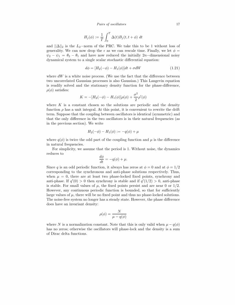
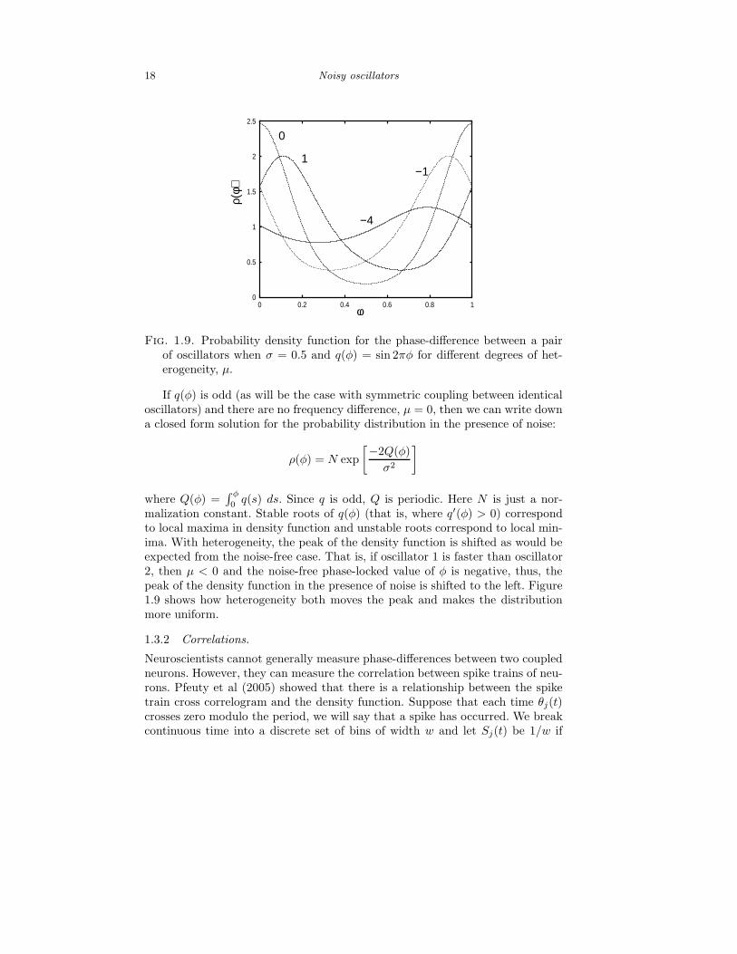
Fig. 1.9. Probability density function for the phase-difference between a pairof oscillators when σ = 0.5 and q(φ) = sin 2πφ for different degrees of het-erogeneity, µ.

If q(φ) is odd (as will be the case with symmetric coupling between identicaloscillators) and there are no frequency difference, µ = 0, then we can write downa closed form solution for the probability distribution in the presence of noise:

ρ(φ) = N exp

[−2Q(φ)

σ2

]

where Q(φ) =∫ φ

0q(s) ds. Since q is odd, Q is periodic. Here N is just a nor-

malization constant. Stable roots of q(φ) (that is, where q′(φ) > 0) correspondto local maxima in density function and unstable roots correspond to local min-ima. With heterogeneity, the peak of the density function is shifted as would beexpected from the noise-free case. That is, if oscillator 1 is faster than oscillator2, then µ < 0 and the noise-free phase-locked value of φ is negative, thus, thepeak of the density function in the presence of noise is shifted to the left. Figure1.9 shows how heterogeneity both moves the peak and makes the distributionmore uniform.

1.3.2 Correlations.

Neuroscientists cannot generally measure phase-differences between two coupledneurons. However, they can measure the correlation between spike trains of neu-rons. Pfeuty et al (2005) showed that there is a relationship between the spiketrain cross correlogram and the density function. Suppose that each time θj(t)crosses zero modulo the period, we will say that a spike has occurred. We breakcontinuous time into a discrete set of bins of width w and let Sj(t) be 1/w if

Pairs of oscillators 19

there is a spike the bin corresponding to t and zero otherwise. The normalizedcross correlation is

C(t2 − t1) :=〈S1(t1)S2(t2)〉〈S1(t)〉〈S2(t)〉

.

Here 〈S(t)〉 is the average of S(t). Pfeuty et al (29) show that as w gets small,

C(τ) ≈ ρ(τ).

Thus, there is simple relationship between the cross-correlation (to lowest order)and the density function of the phase-difference.

1.3.3 Pulse coupling.

In the above parts of this section, we considered additive noise merged withweak coupling of oscillators. However, in an earlier part of this chapter, we alsoshowed that the phase resetting curve is subject to uncertainty in the form ofphase-dependent noise. Thus, consider two neurons which are coupled via phaseresetting curves (in the sense of Goel and Ermentrout (15)):

θ′j = ω +∑

n

B(θj , zj)δ(t− tkn).

Here tkn are the times that oscillator k fires (crosses 0 modulo its period). B(θ, z)is the phase resetting curve parametrized by a random variable, z taken fromsome distribution. Recall from equation (1.14) that the PRC can have phase-dependent variance, so this model might incorporate this variance. If we considertwo identical mutually coupled cells, the phase, φ of cell 2 at the moment cell 1fires satisfies

φn+1 = G(G(φn, zn))

where G(x, z) = 1−x−B(x, z) (see for example, (15; 10)). Here we have assumeda period of 1. Let us write B(x, z) = ǫ∆(x) + zR(x) so that there is possiblyphase-dependent noise, R and a deterministic coupling via the PRC, ǫ∆(x). Asin section 2.2, we can use the theory of stochastic maps to derive an equationfor the invariant density:

P (x) =

∫

∞

−∞

Q([x+ y + ǫ∆(y)]/R(y))

R(y)P (y) dy, (1.22)

where Q(z) is the density of the variable z defined on the real line. We seeksolutions to this equation when P (x + 1) = P (x). Notice that we can wrap theline up as an bi-infinite sum over the unit interval using the periodicity of ∆(x),but for the purposes of analysis, it is much easier to keep the integral over R. IfR(x) = 1+ ǫr(x) and ǫ is small, it is possible to write a formula for the invariant

20 Noisy oscillators

density, P (x) in a perturbation expansion in ǫ. For example, if r(x) = 0 and∆(x) = b1 sin 2πx, then

P (x) ≈ 1 − ǫ2πb1q1

1 − q1cos 2πx

where qn =∫

∞

−∞Q(x) cos 2πx dx. The shape of P (x) is not surprising. If b1 > 0,

then there is a peak at x = 1/2, corresponding to antiphase oscillations whilefor b1 < 0, the peak is at synchrony. Suppose that the noise amplitude is nowphase-dependent and suppose the coupling tends to push the oscillators towardthe antiphase solution (x = 1/2). Let R(x) be such that the variance is minimalnear x = 0, 1 and maximal near x = 1/2. Then, for strong enough noise, onemight expect that the antiphase state might become unstable. That is, eventhough the deterministic dynamics push the oscillators toward antiphase, thePRC is so noisy near that state that the oscillators cannot remain there. Figure1.10 shows an example of this. We take ∆(x) = b sin 2πx andR(x) = 1+c cos 2πx,with b = 0.05 so that the deterministic system has a stable antiphase solutionsand c = −0.4 so that the PRC is noisiest at x = 1/2. For low values of noise,σ = 0.1, Monte-Carlo simulations show a peak at x = 1/2 as predicted from thedeterministic dynamics. However, for σ = 0.35, the histogram of phases showspeaks at 0, 1 corresponding to synchrony. Using the ǫ small approximation forthe invariant density, we find that

P (x) = 1 − 2πǫq1

1 − q1(b + πσ2c) cos 2πx.

Whether the peak is at 1/2 or 0, 1 dependes only on the sign of b+ πσ2c. Thus,there will be a change in the peak if b, c have opposite signs and the noise is largeenough. For our case, the critical value of σ is about 0.25. Figure 1.10B showsthe stationary solutiions to equation (1.22) as a function of σ for ǫ = 1 via acolor code. The switch from a peak at x = 1/2 to x = 0, 1 is evident.

In conclusion, we have shown that for pulse coupling, noise can have a qual-itative effect on the steady state phase distribution if there is phase-dependentvariance in the PRC. For weak coupling, uncorrelated noise does not have morethan a quantitative effect on the behavior of coupled pairs of oscillators. As ex-pected, the phase-differences between the oscillators stay close to the noise-freecase in the sense that stable locked states correspond to peaks in the probabilitydensity. What is interesting is that the peaks remain in the presence of hetero-geneities for case in which the deterministic dynamics do not have phase-lockedsolutions. (E.g., figure 1.9, µ = −4.) Interactions between correlated noise andcoupling is the subject of some of our recent research and should prove to beinteresting.

1.4 Networks of oscillators.

We close this chapter with a sketch of the kinds of analysis that can be donewith large systems of coupled oscillators in the presence of noise and possibly

Networks of oscillators. 21

0

50

100

150

200

250

300

350

400

0 0.2 0.4 0.6 0.8 1

σ=0.1

σ=0.3

1.7

0.2

σ=0.15

σ=0.35

x=0 x=1

x

P(x

)

P(x)

A B

Fig. 1.10. Noise-induced bifurcation in a system with phase-dependent vari-ance. ∆(x) = b sin 2πx, R(x) = (1+c cos 2πx) with b = 0.05, c = −0.25, ǫ = 1for different values of σ. (A) Monte carlo simulation of phase equations with20000 spikes. (B) Steady state density as σ increases from 0.15 to 0.35. Peakin middle disappears whicle a pair of peaks appears at synchrony.

heterogeneities. Kuramoto (22) and later Strogatz (37), Crawford (7), and morerecently, Buice and Chow (6) have studied the behavior of globally coupled oscil-lators in the presence of heterogeneities and noise. (6) consider finite size effects,while the others are interested in the infinite size limit. As the latter case isconsiderable easier to understand and analyze, we only consider this. A very ex-tensive review of the analysis of the Kuramoto model and its generalizations canbe found in Acebron et al (1). Here, we sketch the population density approach(37).

Consider the generalization of equation (1.20) after we have averaged andrescaled time:

dψj = (ωj +1

N

N∑

k=1

H(ψk − ψj))dt+ σdWj(t) (1.23)

where we assume that all oscillators are symmetrically coupled to each otherand that they all have independent noise. As it will be notationally easier, weassume that the period of H is 2π. Kuramoto studies the case in which σ = 0and H(φ) = sinφ as well as the case of no heterogeneity but nonzero noise. Thereview paper (1) references dozens of papers on the analysis of the Kuramotomodel and its descendants. As N → ∞, the ansatz of the population densitymethod is that there is a function, P (θ, ω, t) describing the probability of findingthe oscillator with natural frequency, ω at phase θ at time t. A nice history ofthis method and its development are found in (38; 37). The sum in equation(1.23) is an average over the other phases and as N → ∞ can be written interms of the density function P as

22 Noisy oscillators

limN→∞

1

N

N∑

k=1

H(φk − φj) =

∫

∞

−∞

∫ 2π

0

g(ω)H(φ− φj)P (φ, ω, t) dφ dω := J(φj , t)

(1.24)where g(ω) is the distribution of the frequencies, ωj . With this calculation, thedensity satisfies:

∂P

∂t= − ∂

∂θ[J(θ, t)P (θ, ω, t)] +D

∂2P

∂θ2, (1.25)

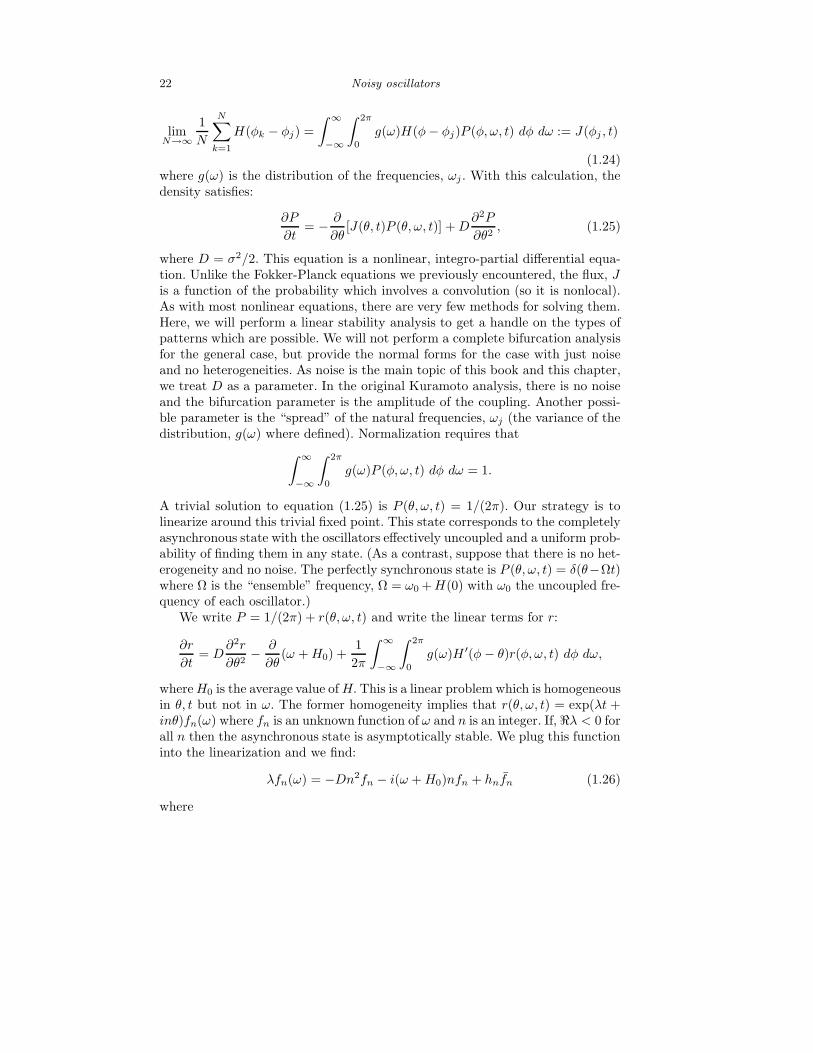
where D = σ2/2. This equation is a nonlinear, integro-partial differential equa-tion. Unlike the Fokker-Planck equations we previously encountered, the flux, Jis a function of the probability which involves a convolution (so it is nonlocal).As with most nonlinear equations, there are very few methods for solving them.Here, we will perform a linear stability analysis to get a handle on the types ofpatterns which are possible. We will not perform a complete bifurcation analysisfor the general case, but provide the normal forms for the case with just noiseand no heterogeneities. As noise is the main topic of this book and this chapter,we treat D as a parameter. In the original Kuramoto analysis, there is no noiseand the bifurcation parameter is the amplitude of the coupling. Another possi-ble parameter is the “spread” of the natural frequencies, ωj (the variance of thedistribution, g(ω) where defined). Normalization requires that

∫

∞

−∞

∫ 2π

0

g(ω)P (φ, ω, t) dφ dω = 1.

A trivial solution to equation (1.25) is P (θ, ω, t) = 1/(2π). Our strategy is tolinearize around this trivial fixed point. This state corresponds to the completelyasynchronous state with the oscillators effectively uncoupled and a uniform prob-ability of finding them in any state. (As a contrast, suppose that there is no het-erogeneity and no noise. The perfectly synchronous state is P (θ, ω, t) = δ(θ−Ωt)where Ω is the “ensemble” frequency, Ω = ω0 +H(0) with ω0 the uncoupled fre-quency of each oscillator.)

We write P = 1/(2π) + r(θ, ω, t) and write the linear terms for r:

∂r

∂t= D

∂2r

∂θ2− ∂

∂θ(ω +H0) +

1

2π

∫

∞

−∞

∫ 2π

0

g(ω)H ′(φ − θ)r(φ, ω, t) dφ dω,

whereH0 is the average value ofH.This is a linear problem which is homogeneousin θ, t but not in ω. The former homogeneity implies that r(θ, ω, t) = exp(λt +inθ)fn(ω) where fn is an unknown function of ω and n is an integer. If, ℜλ < 0 forall n then the asynchronous state is asymptotically stable. We plug this functioninto the linearization and we find:

λfn(ω) = −Dn2fn − i(ω +H0)nfn + hnfn (1.26)

where

Networks of oscillators. 23

fn =

∫

∞

−∞

g(ω)fn(ω) dω

and

hn =1

2π

∫ 2π

0

H ′(φ) exp(inφ) dφ.

Note that hn is the nth Fourier coefficient of the derivative of the H function.We can solve equation (1.26) for fn(ω):

fn(ω) =hnfn

λ+Dn2 + in(H0 + ω).

We plug this into the definition of fn to obtain:

fn = fn

∫

∞

−∞

g(ω)hn

λ+Dn2 + in(H0 + ω)dω.

This equation has a nontrivial solution for fn if and only if

1 =

∫

∞

−∞

g(ω)hn

λ+Dn2 + in(H0 + ω)dω := Γ(λ). (1.27)

Equation (1.27) is the eigenvalue equation that must be solved and the valuesof λ determine stability. The simplest scenario and the only one which we solvehere is when all oscillators are identical and g(ω) is a Dirac delta function at ω0.In this case, the integral is easy to evaluate and we find after trivial algebra:

λ = hn −Dn2 − i(ω0 +H0)n. (1.28)

There is always a zero eigenvalue (n = 0) corresponding to translation invarianceof the phases. For n 6= 0, since hn are bounded, for sufficient noise, D, ℜλ isnegative and the asynchronous state is asymptotically stable. (When there isheterogeneity and no noise, the spectral equation is extremely subtle and theanalysis complex. As there is always noise in neural systems, we make life easyby assuming D > 0.) Suppose that we write

H(φ) = H0 +

∞∑

n=1

an cosnφ+ bn sinnφ.

Thenhn = −inan/2 + nbn/2

thus, the real part of λ is

ℜλ = −Dn2 + nbn/2.

The only terms in H which can destabilize the asynchronous state are those forwhich the Fourier sine coefficients are positive. The critical value of noise is thus

24 Noisy oscillators

D∗ = maxn>0

bn2n

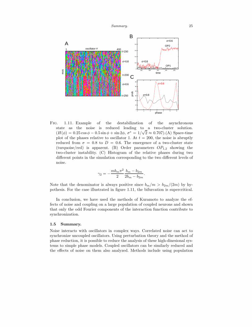
Figure 1.11 shows an example of the application of this analysis to a simulationof 400 globally coupled oscillators. Here H(φ) = 0.25 cosφ − 0.5 sinφ + sin 2φ.The critical value of D predicted is 1/4 corresponding to σ = 1/

√2. We let the

simulation run to steady state with σ = 0.8 (above criticality) and then changedσ to 0.6 which is below the critical value. Figure 1.11A shows a space-time plot ofthe 400 oscillators as a function of time. Their phases relative to oscillator 1 areplotted in a color code over a time window including the decrease of the noiseamplitude. The color coding shows that after the noise is reduced, oscillatorsare divided into roughly two clusters (pink and blue) corresponding to a 0 andπ phase-differences. This is a two cluster state. We introduce so-called “orderparameters”, which quantify the degree of synchrony between the oscillators:

OPn :=1

N

√

√

√

√

√

N∑

j=1

cosnθj

2

+

N∑

j=1

sinnθj

2

.

These pick out the Fourier coefficients of the invariant density, P (θ, ω, t) andvanish when the oscillators are asynchronous. If D < bn/n, we expect OPn togrow. Figure 1.11B shows the abrupt change in OP2 as predicted from the infiniteN theory. Figure 1.11C shows histograms at the high and low noise levels forone time slice of the 400 oscillators. There are two clear peaks in the low noisecase as predicted from the linear analysis.

A natural, next approach to the equation is to do a full nonlinear bifurcationanalysis. This was done in chapter 5 of Kuramoto. The first step is to subtractoff the constant frequency and the constant Fourier term of H . Thus, we reduce(1.25) to the following nonlinear equation:

∂P

∂t= − ∂

∂θ

∫ 2π

0

H(φ− θ)P (θ, t)P (φ, t) dφ+D∂2P

∂θ2.

Letting m denote the critical wave number, the normal form for the bifurcationhas the form:

zt = z[m2(D∗ −D) + γ2zz]

where

γ2 = −mπ2

2

(

b2m + a2m + ama2m − bmb2m + i(a2mbm + amb2m)

2bm − b2m + i(a2m − am)

)

andH(φ) =

∑

n

an cosnφ+ bm sinnφ.

The bifurcation is supercritical if the real part of γ2 is negative. Note that if Hcontains only odd periodic terms then

Summary. 25

0

0.2

0.4

0.6

0.8

160 180 200 220 240

0

10

20

30

40

50

60

0 1 2 3 4 5 6

prob

phase

OP2

OP1

t=150

time

t=250

t=200

1 400oscillator #

time

σ=0.8

σ=0.6

σ=0.8

σ=0.6

σ=0.8

σ=0.6

AB

C

Fig. 1.11. Example of the destabilization of the asynchronousstate as the noise is reduced leading to a two-cluster solution.(H(φ) = 0.25 cosφ − 0.5 sinφ + sin 2φ, σ∗ = 1/

√2 ≈ 0.707).(A) Space-time

plot of the phases relative to oscillator 1. At t = 200, the noise is abruptlyreduced from σ = 0.8 to D = 0.6. The emergence of a two-cluster state(turquoise/red) is apparent. (B) Order parameters OP1,2 showing thetwo-cluster instability. (C) Histogram of the relative phases during twodifferent points in the simulation corresponding to the two different levels ofnoise.

γ2 = −mbmπ2

2

bm − b2m

2bm − b2m

.

Note that the denominator is always positive since bm/m > b2m/(2m) by hy-pothesis. For the case illustrated in figure 1.11, the bifurcation is supercritical.

In conclusion, we have used the methods of Kuramoto to analyze the ef-fects of noise and coupling on a large population of coupled neurons and shownthat only the odd Fourier components of the interaction function contribute tosynchronization.

1.5 Summary.

Noise interacts with oscillators in complex ways. Correlated noise can act tosynchronize uncoupled oscillators. Using perturbation theory and the method ofphase reduction, it is possible to reduce the analysis of these high-dinesional sys-tems to simple phase models. Coupled oscillators can be similarly reduced andthe effects of noise on them also analyzed. Methods include using population

26 Noisy oscillators

density equations, Fokker-Planck equations, and the analysis of linear integraloperators. There are many unanswered questions such as what happens withlarger noise and how interactions between internal dynamics and correlated in-puts change the ability to synchronize.

REFERENCES

J. A. Acebron, L. L. Bonilla, C. J. Perez Vicente, F. Ritort and R. Spigler, TheKuramoto model: a simple paradigm for synchronization phenomena. Rev.Mod. Phys. 77, 137-185 (2005).

Brown, E, Moehlis, J, and Holmes, P, On the phase reduction and responsedynamics of neural oscillator populations. Neural Computation 16:673-715,2004

Brette R, Guigon E. Reliability of spike timing is a general property of spikingmodel neurons. Neural Comput. 2003 Feb;15(2):279-308

Brette R. Dynamics of one-dimensional spiking neuron models. J Math Biol.2004 Jan;48(1):38-56.

Bryant HL, Segundo JP. Spike initiation by transmembrane current: a white-noise analysis. J Physiol 260:279-314, 1975

Buice MA, Chow CC Correlations, fluctuations, and stability of a finite-sizenetwork of coupled oscillators PHYSICAL REVIEW E 76 (3): Art. No.031118

Crawford, J. D. Amplitude Expansions for Instabilities in Populations of Globally-Coupled Oscillators, 1994, J. Stat. Phys. 74, 1047

Engen S, Saether BE, Generalizations of the Moran effect explaining spatialsynchrony in population fluctuations, Am Nat. 166:603-12 2005

Ermentrout, B. Type I membranes, phase resetting curves, and synchrony. Neu-ral Comput. 8 (1996), pp. 979-1001

Ermentrout B, Saunders D Phase resetting and coupling of noisy neural oscil-lators JCNS 20: 179-190, 2006

Fernandez Galan R, Ermentrout GB, Urban NN. Stochastic dynamics of uncou-pled neural oscillators: Fokker-Planck studies with the finite element methodPhys. Rev. E 76, 056110 (2007)

Galan RF, Ermentrout GB, Urban NN. Efficient estimation of phase-resettingcurves in real neurons and its significance for neural-network modeling. PhysRev Lett 94: 158101, 2005.

Galan RF, Fourcaud-Trocme N, Ermentrout GB, Urban NN. Correlation-inducedsynchronization of oscillations in olfactory bulb neurons. J Neurosci. 2006Apr 5;26(14):3646-55.

Galan R F, Ermentrout GB, Urban NN. Optimal time scale for spike-timereliability: Theory, simulations and experiments. J Neurophysiol 99:277-283,2008

Goel,P and Ermentrout, B, Synchrony, stability, and firing patterns in pulse-coupled oscillators , Physica D 163:191-216, 2002

Goldobin DS, Pikovsky A, Synchronization and desynchronization of self-sustainedoscillators by common noise, PRE 71:045201,2005

28 References

J. Guckenheimer (1975). Isochrons and phaseless sets, J. Math. Biol., 1: 259-273.Gutkin BS, Ermentrout GB, Reyes AD Phase-response curves give the re-

sponses of neurons to transient inputs J. Neurophys. 94: 1623-1635, 2005D. Hansel, G. Mato and C. Meunier , Synchrony in excitatory neural networks.

Neural Comput. 7 (1995), pp. 307-337Izhikevich E.M., Dynamical Systems in Neuroscience: The Geometry of Ex-

citability and Bursting, MIT Press, Cambridge, MA, 2007Jensen RV, Synchronization of driven nonlinear oscillators, AMERICAN JOUR-

NAL OF PHYSICS 70 (6): 607-619 JUN 2002. Kuramoto, Y., Chemical Oscillations, Waves, and Turbulence, Springer, Berlin,

1984Lasota A, Mackey MC (1986) Chaos, Fractals and Noise: Stochastic Aspects

of Dynamics, Springer Applied Mathematical Science 97. Springer-Verlag,Berlin (Chapt. 10.5).

Lindner B, Longtin A, Bulsara A. Analytic expressions for rate and CV of a typeI neuron driven by white gaussian noise. Neural Comput. 2003 15:1760-87

Mainen ZF, Sejnowski TJ. Reliability of spike timing in neocortical neurons.Science 268: 1503-1506, 1995

Marella, S and Ermentrout, GB, Type II neurosn display a higher degree ofstochastic synchronization compared to Type I, (submitted).

Nakao H, Arai K, Kawamura Y. Noise-induced synchronization and clusteringin ensembles of uncoupled limit-cycle oscillators Phys Rev Lett. 2007 May4;98(18):184101. Epub 2007 May 2.

Netoff TI, Banks MI, Dorval AD, Acker CD, Haas JS, Kopell N, White JA.Synchronization in hybrid neuronal networks of the hippocampal formation.J Neurophysiol. 2005 Mar;93(3):1197-208. Epub 2004 Nov 3.

Pfeuty B, Mato G, Golomb D, Hansel D. Electrical synapses and synchrony: therole of intrinsic currents. J Neurosci. 2003 Jul 16;23(15):6280-94. Erratumin: J Neurosci. 2003 Aug 6;23(18):7237.

Pikovsky A.S. Synchronization and stochastization of the ensamble of autogen-erators by external noise, Radiophys.Quantum Electron., 27, n.5, 576-581,1984.

Pikovsky, A, Rosenblum, M, and Kurths, J. Synchronization: A Universal Con-cept in Nonlinear Sciences, Cambridge University Press, 2001

Reyes AD, Fetz EE, Effects of transient depolarizing potentials on the firingrate of cat neocortical neurons, J Neurophysiol.69:1673-83, 1993

Risken, H. The Fokker-Planck Equation (Chapt 7), Springer NY 1996.Ritt J. Evaluation of entrainment of a nonlinear neural oscillator to white noise.

Phys Rev E Stat Nonlin Soft Matter Phys. 2003 Oct;68(4 Pt 1):041915.Stratonovich, RL, Oscillator synchronization in the presence of noise, Ra- diotekhnika

i elektronika 3 (1958) 497, english translation in Non-linear trans- forma-tions of stochastic processes, edited by P. I. Kuznetsov, R. L Stratonovich,V. I. Tikhonov, Pergamon Press, Oxford 1965.

Stratonovich, RL, Theory of Random Noise, Gordon and Breach, 1969.

References 29

Strogatz,SH From Kuramoto to Crawford: exploring the onset of synchroniza-tion in populations of coupled oscillators Physica D:143, 2000,1-20

Strogatz, S.H., Sync: The Emerging Science of Spontaneous Order, PenguinBooks Ltd, 2004

Tateno T, Robinson HP, Phase resetting curves and oscillatory stability ininterneurons of rat somatosensory cortex, Biophy. J. 92:683-95, 2007

Teramae JN, Tanaka D. Robustness of the noise-induced phase synchroniza-tion in a general class of limit cycle oscillators. Phys Rev Lett. 2004 Nov12;93(20):204103. Epub 2004 Nov 12.

Troyer TW. Factors affecting phase synchronization in integrate-and-fire oscil-lators. J Comput Neurosci. 2006 Apr;20(2):191-200.

Tsubo Y, Takada M, Reyes AD, Fukai T, Layer and frequency dependencies ofphase response properties of pyramidal neurons in rat motor cortex, Eur JNeurosci. 25:3429-41, 2007.

A. T. Winfree (2001). The geometry of biological time (2nd edition). Springer-Verlag.

Zhou T, Chen L, Aihara K, Molecular communication through stochastic syn-chronization induced by extracellular fluctuations, PRL 95:178103, 2005

Mainen, Z.F. and Sejnowski, T.J. (1995) Reliability of spike timing in neocor-tical neurons Science, 268:1503 - 1506