Stochastic Networks in Nanoscale Biophysics: …skou/papers/stochnet-JASA.pdfStochastic Networks in...
15
Stochastic Networks in Nanoscale Biophysics: Modeling Enzymatic Reaction of a Single Protein S. C. KOU Advances in nanotechnology enable scientists for the first time to study biological processes on a nanoscale molecule-by-molecule basis. A surprising discovery from recent nanoscale single-molecule biophysics experiments is that biological reactions involving enzymes behave fundamentally differently from what classical theory predicts. In this article we introduce a stochastic network model to explain the experi- mental puzzles (by modeling enzymatic reactions as a stochastic network connected by different enzyme conformations). Detailed analyses of the model, including analyses of the first-passage-time distributions and goodness of fit, show that the stochastic network model is capa- ble of explaining the experimental surprises. The model is analytically tractable and closely fits experimental data. The biological/chemical meaning of the model is discussed. KEY WORDS: Autocorrelation function; Continuous-time Markov chain; First passage time; Goodness of fit; Maximum likelihood esti- mates; Michaelis–Menten model; Reaction rate. 1. INTRODUCTION The rapid advances in nanotechnology have generated much excitement in the scientific and engineering communities. Its application to the biological front in the last two decades led to the new field of nanoscale biophysics: Scientists for the first time were able to study biological processes on an unprece- dented nanoscale molecule-by-molecule basis (Nie and Zare 1997; Xie and Trautman 1998; Xie and Lu 1999; Tamarat, Maali, Lounis, and Orrit 2000; Weiss 2000; Moerner 2002; Kou, Xie, and Liu 2005b). This new development has opened the door to addressing many problems that were inaccessi- ble just a few decades ago and has attracted much attention from biologists, chemists, and biophysicists, because nanoscale single-molecule experiments offer many advantages over the traditional experiments involving a population of molecules. First, by allowing scientists to “zoom in” on individual mole- cules, single-molecule experiments provide data with more ac- curacy and higher resolution. Second, by isolating, tracking, and manipulating individual molecules, single-molecule exper- iments capture transient intermediates and detailed dynamics of a biological process, the type of information rarely available from traditional population experiments. Third, by following single molecules, scientists can study biological processes di- rectly on the individual molecule level, instead of relying on the extremely difficult task of synchronizing the actions of a population of biomolecules. Fourth, because many important biological functions in a living cell are performed by single molecules, understanding the behavior of individual biomole- cules is a crucial task, for which single-molecule experiments are specifically designed. Many new scientific discoveries (see, e.g., Lu, Xun, and Xie 1998; Zhuang et al. 2002; Asbury, Fehr, and Block 2003; Yang et al. 2003; Kou and Xie 2004; Kou et al. 2005a) have emerged from the nanoscale single-molecule studies. Advances in nanoscale single-molecule biophysics also bring opportunities for statisticians and probabilists because to char- acterize the behavior of individual molecules, which exist in the nanometer world subject to the laws of statistical and quantum S. C. Kou is John L. Loeb Associate Professor of the Natural Sciences, Department of Statistics, Harvard University, Cambridge, MA 02138 (E-mail: [email protected]). The author thanks the Xie group of the Department of Chemistry and Chemical Biology of Harvard University for sharing the experi- mental data and for fruitful discussions. The research was supported in part by NSF Career Award DMS-0449204. mechanics, stochastic models and their statistical inference are indispensable (Kou 2008). In this article we consider recent single-molecule experi- ments on enzymatic reactions (Flomembom et al. 2005; Eng- lish et al. 2006), where the high-resolution experimental results showed a surprising departure from what classical theory pre- dicts. To explain the single-molecule experimental findings, we introduce a stochastic network model to describe the enzymatic reaction kinetics. According to the classical Michaelis–Menten (MM) model of enzymatic reaction in biochemistry (Atkins and de Paula 2002), an enzyme catalyzes a reaction in the following way. First, the enzyme binds to the reactant, which is referred to in the biochemistry literature as a substrate, and forms an enzyme– substrate complex. The complex then undergoes a decomposi- tion to generate the reaction product and release the enzyme in its original form to catalyze the next substrate. In the biochem- istry literature this process is typically diagrammed as E + S ES → E 0 + P, E 0 → E, where the arrows indicate the reaction direction and E (and E 0 ), S , ES, and P stand for the enzyme, the substrate, the enzyme–substrate complex, and the reaction product, respec- tively. In addition to providing a schematic picture, the classical MM model also gives quantitative results; for example, it ex- plicitly describes how the reaction rate depends on the substrate concentration (see Sec. 2 for details). Over the years, numer- ous experiments carried out in the traditional way (i.e., using a population of enzymes and substrates) yielded results agree- ing with the quantitative descriptions of the MM model, and, thus, for decades the MM model was featured in textbooks as the fundamental mechanism for enzymatic reactions (Hammes 1982; Fersht 1985; Segel 1993). Recent nanoscale single-molecule experiments (English et al. 2006), which for the first time tracked the behavior of a sin- gle enzyme, however, have surprised researchers, as the high- resolution experimental data showed an unequivocal departure from the MM model: © 2008 American Statistical Association Journal of the American Statistical Association September 2008, Vol. 103, No. 483, Applications and Case Studies DOI 10.1198/016214507000001021 961
Transcript of Stochastic Networks in Nanoscale Biophysics: …skou/papers/stochnet-JASA.pdfStochastic Networks in...

Stochastic Networks in Nanoscale Biophysics:Modeling Enzymatic Reaction of a Single Protein
S. C. KOU
Advances in nanotechnology enable scientists for the first time to study biological processes on a nanoscale molecule-by-molecule basis.A surprising discovery from recent nanoscale single-molecule biophysics experiments is that biological reactions involving enzymes behavefundamentally differently from what classical theory predicts. In this article we introduce a stochastic network model to explain the experi-mental puzzles (by modeling enzymatic reactions as a stochastic network connected by different enzyme conformations). Detailed analysesof the model, including analyses of the first-passage-time distributions and goodness of fit, show that the stochastic network model is capa-ble of explaining the experimental surprises. The model is analytically tractable and closely fits experimental data. The biological/chemicalmeaning of the model is discussed.
KEY WORDS: Autocorrelation function; Continuous-time Markov chain; First passage time; Goodness of fit; Maximum likelihood esti-mates; Michaelis–Menten model; Reaction rate.
1. INTRODUCTION
The rapid advances in nanotechnology have generated muchexcitement in the scientific and engineering communities. Itsapplication to the biological front in the last two decades ledto the new field of nanoscale biophysics: Scientists for the firsttime were able to study biological processes on an unprece-dented nanoscale molecule-by-molecule basis (Nie and Zare1997; Xie and Trautman 1998; Xie and Lu 1999; Tamarat,Maali, Lounis, and Orrit 2000; Weiss 2000; Moerner 2002;Kou, Xie, and Liu 2005b). This new development has openedthe door to addressing many problems that were inaccessi-ble just a few decades ago and has attracted much attentionfrom biologists, chemists, and biophysicists, because nanoscalesingle-molecule experiments offer many advantages over thetraditional experiments involving a population of molecules.First, by allowing scientists to “zoom in” on individual mole-cules, single-molecule experiments provide data with more ac-curacy and higher resolution. Second, by isolating, tracking,and manipulating individual molecules, single-molecule exper-iments capture transient intermediates and detailed dynamicsof a biological process, the type of information rarely availablefrom traditional population experiments. Third, by followingsingle molecules, scientists can study biological processes di-rectly on the individual molecule level, instead of relying onthe extremely difficult task of synchronizing the actions of apopulation of biomolecules. Fourth, because many importantbiological functions in a living cell are performed by singlemolecules, understanding the behavior of individual biomole-cules is a crucial task, for which single-molecule experimentsare specifically designed. Many new scientific discoveries (see,e.g., Lu, Xun, and Xie 1998; Zhuang et al. 2002; Asbury, Fehr,and Block 2003; Yang et al. 2003; Kou and Xie 2004; Kou etal. 2005a) have emerged from the nanoscale single-moleculestudies.
Advances in nanoscale single-molecule biophysics also bringopportunities for statisticians and probabilists because to char-acterize the behavior of individual molecules, which exist in thenanometer world subject to the laws of statistical and quantum
S. C. Kou is John L. Loeb Associate Professor of the Natural Sciences,Department of Statistics, Harvard University, Cambridge, MA 02138 (E-mail:[email protected]). The author thanks the Xie group of the Department ofChemistry and Chemical Biology of Harvard University for sharing the experi-mental data and for fruitful discussions. The research was supported in part byNSF Career Award DMS-0449204.
mechanics, stochastic models and their statistical inference areindispensable (Kou 2008).
In this article we consider recent single-molecule experi-ments on enzymatic reactions (Flomembom et al. 2005; Eng-lish et al. 2006), where the high-resolution experimental resultsshowed a surprising departure from what classical theory pre-dicts. To explain the single-molecule experimental findings, weintroduce a stochastic network model to describe the enzymaticreaction kinetics.
According to the classical Michaelis–Menten (MM) modelof enzymatic reaction in biochemistry (Atkins and de Paula2002), an enzyme catalyzes a reaction in the following way.First, the enzyme binds to the reactant, which is referred to inthe biochemistry literature as a substrate, and forms an enzyme–substrate complex. The complex then undergoes a decomposi-tion to generate the reaction product and release the enzyme inits original form to catalyze the next substrate. In the biochem-istry literature this process is typically diagrammed as
E + S � ES → E0 + P, E0 → E,
where the arrows indicate the reaction direction and E (andE0), S, ES, and P stand for the enzyme, the substrate, theenzyme–substrate complex, and the reaction product, respec-tively.
In addition to providing a schematic picture, the classicalMM model also gives quantitative results; for example, it ex-plicitly describes how the reaction rate depends on the substrateconcentration (see Sec. 2 for details). Over the years, numer-ous experiments carried out in the traditional way (i.e., usinga population of enzymes and substrates) yielded results agree-ing with the quantitative descriptions of the MM model, and,thus, for decades the MM model was featured in textbooks asthe fundamental mechanism for enzymatic reactions (Hammes1982; Fersht 1985; Segel 1993).
Recent nanoscale single-molecule experiments (English etal. 2006), which for the first time tracked the behavior of a sin-gle enzyme, however, have surprised researchers, as the high-resolution experimental data showed an unequivocal departurefrom the MM model:
© 2008 American Statistical AssociationJournal of the American Statistical Association
September 2008, Vol. 103, No. 483, Applications and Case StudiesDOI 10.1198/016214507000001021
961

962 Journal of the American Statistical Association, September 2008
• First, under the MM model a single enzyme behaves asa continuous-time Markov chain, switching among thethree states E, ES, and E0. From the Markov descrip-tion, the MM model predicts that an enzyme’s turnovertime, which is the time that it takes the enzyme to com-plete one catalytic cycle (i.e., to go from state E to stateE0), should have (almost) a purely exponential distrib-ution. The single-molecule experimental data, however,show that the distribution of the turnover time is actuallymuch heavier than an exponential one.
• Second, because under the MM model a single enzymebehaves as a continuous-time Markov chain, it followsfrom the Markov property that an enzyme’s successiveturnover times should be independently and identicallydistributed. In the single-molecule experiments, however,it is observed that a single enzyme’s successive turnovertimes are, in fact, highly correlated, possessing a strongmemory.
• Third, the MM model gives a formula (known as theMichaelis–Menten equation in the literature) that displaysa hyperbolic relationship between the reaction rate and thesubstrate concentration. This formula appears to hold forthe single-molecule experimental data.
Sections 2 and 5 will provide more details. Some questionsimmediately arise from these observations. First, what causesthe turnover time’s heavier-than-exponential distribution? Sec-ond, how can an enzyme “remember” its past, and from wheredoes the memory come? Third, given that the experimentaldata have contradicted the two fundamental predictions of theMM model, how can the explicit formula derived from the MMequation still hold?
We formulate a stochastic network model to answer thesequestions.
From a statistics standpoint, we conduct a detailed analysis ofthe stochastic network: studying its statistical inference as wellas analyzing the first passage times on the network, as both arecrucial in explaining the experimental puzzles.
From an application point of view, we show that by utilizinga stochastic network structure to describe enzymatic reactionkinetics at the molecular level, the recent experimental puzzlescan be satisfactorily resolved.
The outline of the article is as follows. Section 2 reviews theexperimental puzzles that motivate our study and introduces ourstochastic network model; special attention is paid to the bio-logical/chemical meaning of the model components. Section 3investigates the properties of the model, the stationary and thefirst-passage-time distributions in particular. The analytical re-sults are applied in Section 4 to explain the experimental puz-zles. Section 5 considers data from recent single-molecule ex-periments, assesses the goodness of fit of the MM model tothe real data, and uses maximum likelihood to fit our modelto the experimental data, showing close agreement between ourmodel and the data. Section 6 concludes the article with a dis-cussion. All the technical derivations and proofs are given inthe Appendix.
2. MODELING ENZYMATIC REACTIONS
2.1 The Classical Michaelis–Menten Model andIts Limitations
To facilitate the introduction of our model, we first reviewthe classical MM model and its limitations in explaining recentsingle-molecule experimental results.
In the MM model, with the substrate concentration held con-stant, a single enzyme molecule cycles repetitively through thethree states E, ES, and E0 via
E + Sk1[S]�k−1
ESk2→ E0 + P, E0 δ→ E, (2.1)
where the symbol [S] denotes the (constant) substrate concen-tration; k1 is the association rate (per unit substrate concentra-tion); k−1 and k2 are, respectively, the dissociation and catalyticrate; and δ is the rate of E0’s return to E.
In our familiar statistics language, diagram (2.1) is the rout-ing map of a three-state continuous-time Markov chain with theinfinitesimal generator (transition matrix)
QMM =(−k1[S] k1[S] 0
k−1 −(k−1 + k2) k2δ 0 −δ
).
An enzyme molecule switches continuously among the threestates E, ES, and E0 according to QMM.
The time needed for an enzyme to complete one catalyticcycle is called the turnover time.
In the MM model the turnover time is the first passage timefrom state E to state E0. The density function of this first pas-sage time is given by the following proposition, whose deriva-tion is deferred to the Appendix.
Proposition 2.1. The density function of the first passagetime from state E to state E0 is
f (t) = k1k2[S]2p
(e−(q−p)t − e−(q+p)t
), (2.2)
where p = √(k1[S] + k2 + k−1)2/4 − k1k2[S] and q =
(k1[S] + k2 + k−1)/2.
Equation (2.2), together with (2.1), has important experimen-tal implications for the MM model.
• First, (2.2) says that the distribution of the turnover timeshould have an exponential decay with rate q − p in theMM model. Furthermore, due to the exponential nature,for most values of t , e−(q−p)t easily overwhelms e−(q+p)t ;thus, f (t) is almost a purely exponential distribution, andwill, thus, yield a practically straight line on a log-linearplot. Figure 1 illustrates this point, plotting f (t) on a log-linear scale for typical values of [S], k1, k2, and k−1; aclear linear pattern is shown.
• Second, because an enzyme’s behavior is modeled as aMarkov chain in the MM model, it follows immediatelythat an enzyme’s successive turnover times are indepen-dently and identically distributed. No memory should befound among the turnover times.

Kou: Stochastic Networks in Nanoscale Biophysics 963
Figure 1. Density function f (t) of the turnover time from the MMmodel plotted on a log-linear scale. [S] = 100 μM (micromolar),k1 = 5 × 10⁷ M−1 s−1, k2 = 730 s−1, k−1 = 18,300 s−1.
• Third, from (2.2) we know that the mean turnover time is∫ ∞
0f (t)t dt = k1[S] + k2 + k−1
k1k2[S] .
The reciprocal of the mean turnover time is defined as theenzymatic reaction rate (Yang and Cao 2001; Kou et al.2005a; Min et al. 2006):
v = 1/(∫ ∞
0f (t)t dt
)= k2[S]
[S] + (k2 + k−1)/k1. (2.3)
This relationship, referred to as the Michaelis–Mentenequation, is of fundamental importance in the biochem-istry literature (Segel 1993; Atkins and de Paula 2002):It gives an explicit hyperbolic dependence of the reactionrate v on the substrate concentration [S].
Before nanoscale single-molecule experiments were possi-ble, numerous researchers had studied different enzyme sys-tems under the traditional experimental approach. Unable tofollow an individual enzyme molecule, the traditional experi-ments relied on a population of enzymes, and by measuring theaccumulation of reaction products over time, researchers esti-mated the reaction rate for various substrate concentrations. Itwas found in these traditional experiments that the hyperbolicform in (2.3), that is,
v ∝ [S]/([S] + C) with some constant C,
appeared to hold for many enzymes. Thus, for decades the MMmodel has been featured in textbooks as the fundamental mech-anism for enzymatic reactions (Hammes 1982; Fersht 1985;Segel 1993).
Advances in nanotechnology have made it possible to studyenzymatic reactions at the single-molecule level. English etal. (2006) recently carried out single-molecule experiments tostudy β-galactosidase, an essential enzyme in the human bodythat catalyzes the breakdown of the sugar lactose (Jacobson,Zhang, DuBose, and Matthews 1994; Dorland 2003). The ex-perimental results surprised researchers, as the high-resolutiondata clearly demonstrated that
a. The empirical distribution of the experimentally recordedturnover times is much heavier than an exponential one.
b. A single enzyme’s successive turnover times are stronglycorrelated.
c. The hyperbolic relationship of v ∝ [S]/([S] + C) appearsto hold true for the single-molecule data.
Section 5 will provide details about the experiments. Giventhat findings (a) and (b) contradict the fundamentals of the MMmodel, finding (c) is even more surprising.
2.2 The Stochastic Network Model
Model Construction. An important clue in our effort to re-solve the experimental puzzles comes from other recent single-molecule experiments (Lu et al. 1998; Yang et al. 2003; Kouand Xie 2004; Min et al. 2005a; Min et al. 2005b), where, instudying different biological systems, researchers have becomeaware that enzymes are not rigid entities but rather dynamicbiomolecules, experiencing constant changes and fluctuationsin their three-dimensional shape and configuration. This obser-vation suggests that we should not treat an enzyme as an objectwith a fixed state; instead, we should view an enzyme as a col-lection of states, each state being a distinct conformation (i.e.,a distinct spatial configuration) with an enzyme spontaneouslyswitching among the different states. With this insight we pro-pose the following stochastic network model for enzymatic re-actions, diagrammed as
S + E1
k11[S]�k−11
ES1k21→ P + E0
1, E01
δ1→ E1,
↓↑ ↓↑ ↓↑ ...
S + E2
k12[S]�k−12
ES2k22→ P + E0
2, E02
δ2→ E2,
......
......
↓↑ ↓↑ ↓↑S + En
k1n[S]�k−1n
ESnk2n→ P + E0
n, E0n
δn→ En,
(2.4)
where E1,E2, . . . represent the different states (conformations)of the original enzyme, and ESi and E0
i are the states corre-sponding to subsequent enzyme–substrate binding and decom-position. The parameter [S] in (2.4) denotes the concentrationof substrate [as in (2.1)]; k1i is the association rate (per unitconcentration) for the ith state Ei ; and k−1i , k2i , and δi are,respectively, the dissociation, catalytic, and returning rates cor-responding to the transitions from ESi to S + Ei , from ESi toP + E0
i , and from E0i to Ei , respectively.
The transitions among the Ei ’s in the model capture the (con-formational) fluctuation of the enzyme. It should be understoodthat Ei not only connects with Ei−1 and Ei+1 but also with allthe other Ej ’s [we only depict the Ei ↔ Ei−1 and Ei ↔ Ei+1transitions in (2.4) due to graphical limitations], and the sameis true among the ESi states and the E0
i states, respectively.Different states, due to their specific spatial arrangement,
could have different reactivity levels. This is embodied in themodel by allowing k1i , k−1i , k2i , and δi to take distinct valuesfor different i.
The transitions between S + Ei and ESi incorporate the in-sight that in a real enzymatic reaction, the enzyme–substratebinding should take place between the substrate and a specificspatial configuration of the enzyme (and in this regard there is

964 Journal of the American Statistical Association, September 2008
no transition between S + Ei and ESj and between ESi and E0j
for i �= j because they correspond to different conformations).Our model (2.4) generalizes the classical MM model to a
stochastic network in the sense of Kelly and Williams (1995),Glasserman, Sigman, and Yao (1996), Chen and Yao (2001),and Ball, Kurtz, Popovic, and Rempala (2006). Each stageof enzymatic reaction (initiation, binding, and decomposition)consists of a collection of states (enzyme conformations). Aswe shall see, this multistates network structure plays a centralrole in explaining the experimental results.
Statistical Formulation. Let αij denote the transition ratefrom Ei to Ej (i �= j ), βij denote the transition rate from ESi toESj , and γij denote the transition rate from E0
i to E0j . Then the
stochastic network (2.4) can be described as a continuous-timeMarkov chain with infinitesimal generator (transition matrix)
Q =(QAA − QAB QAB 0
QBA QBB − (QBA + QBC) QBC
QCA 0 QCC − QCA
),
(2.5)
where for notational convenience the square matrix QAA rep-resents the transition rates among the Ei states (think of Ai asshorthand notation for Ei ),
(QAA)ij = αij for i �= j, (QAA)ii = −∑j �=i
αij .
Likewise, the matrices QBB and QCC represent the transitionrates among the ESi states and E0
i states, respectively (think ofBi and Ci as shorthand notation for ESi and E0
i , respectively),
(QBB)ij = βij for i �= j, (QBB)ii = −∑j �=i
βij ,
(QCC)ij = γij for i �= j, (QCC)ii = −∑j �=i
γij .
The diagonal matrices QAB , QBA, QBC , and QCA in (2.5)denote the transition rates from Ei to ESi , from ESi to Ei ,from ESi to E0
i , and from E0i to Ei , respectively: QAB =
diag(k11[S], k12[S], . . . , k1n[S]), QBA = diag(k−11, k−12, . . . ,
k−1n), QBC = diag(k21, k22, . . . , k2n), and QCA = diag(δ1, δ2,
. . . , δn).
Turnover Time. In our model (2.4) an enzyme’s turnovertime is the first passage time from the first reaction stage tothe third stage, that is, from any Ei state to any E0
j state.For example, suppose an enzyme travels through the followingpath: E0
1 → E1 → E2 → ES2 → E02 → E2 → E3 → ES3 →
ES1 → S1 → ES1 → E01 . Then the first turnover time corre-
sponds to E1 → E2 → ES2 → E02 , and the second corresponds
to E2 → E3 → ES3 → ES1 → S1 → ES1 → E01 . The feature
that a turnover event can start from any Ei and end in any E0j
in our model captures the fact that in a single-molecule exper-iment, instead of observing the specific enzyme conformationsand their interconversions, one can record only the time for anenzyme to complete a reaction cycle. In other words, on thenetwork (2.4), the exact states are not observed, and only tran-sitions from the first stage (consisting of E1, . . . ,En) to the laststage (consisting of E0
1, . . . ,E0n) are observed.
3. PROPERTIES OF THE STOCHASTICNETWORK MODEL
We study the stochastic network model in this section. Theresults will be used in Section 4 to explain the experimentalpuzzles.
3.1 Detailed Balance: A Constraint on the Model
An important chemical requirement for kinetic models is thedetailed balance condition (Lewis 1925; Schnakenberg 1976;Kelly 1979). It states that if any two states are mutually spon-taneously convertible, then detailed balance must hold betweenthem. In our case, because Ei and Ej are mutually convert-ible, and so are the pairs ESi and ESj , E0
i , and E0j , and Ei and
ESi , the transition rates must satisfy the following constraints:There exist positive numbers φ(Ei), φ(ESi ), and φ(E0
i ) (i =1,2, . . . , n) such that, for any i and j ,
φ(Ei)αij = φ(Ej )αji, φ(ESi )βij = φ(ESj )βji,(3.1)
φ(Ei)k1i[S] = φ(ESi )k−1i , φ(E0i )γij = φ(E0
j )γji .
In matrix notation the detailed balance condition can be con-cisely written as(
�A 00 �B
)(QAA QAB
QBA QBB
)
=(
QAA QAB
QBA QBB
)T (�A 00 �B
), (3.2)
�CQCC = QTCC�C,
where the diagonal matrices �A = diag(φ(E1),φ(E2), . . . ,
φ(En)), �B = diag(φ(ES1), . . . , φ(ESn)), and �C =diag(φ(E0
1), . . . , φ(E0n)).
The detailed balance condition (3.1) implies, in particular,that if we isolate the Ei states (i = 1,2, . . . , n) and look only attransitions among them, that is, if we look at the subnetwork of(2.5) with transition matrix QAA, then
φA = (φ(E1),φ(E2), . . . , φ(En)
)(3.3)
is the stationary measure for the subnetwork: φAQAA = 0. Sim-ilarly, for ESi states in isolation, and E0
i states in isolation
φB = (φ(ES1), . . . , φ(ESn)
)and
(3.4)φC = (
φ(E01), . . . , φ(E0
n))
are the stationary measures for the subnetworks, respectively:φBQBB = 0, φCQCC = 0. Furthermore, if we consider the sub-network consisting of Ei and ESi states (i = 1,2, . . . , n) to-
gether [which has(
QAA − QAB QAB
QBA QBB − QBA
)as the transition ma-
trix], (φA,φB) is the stationary measure:
(φA,φB)
(QAA − QAB QAB
QBA QBB − QBA
)= 0.
On the other hand, because ESi and E0i are not mutually con-
vertible, there is no detailed balance between them, and, in gen-eral, (φA,φB,φC) is not the stationary measure of the entirenetwork: (φA,φB,φC)Q �= 0.

Kou: Stochastic Networks in Nanoscale Biophysics 965
Remark 1. It is worth emphasizing that in our model detailedbalance holds only for subnetworks, not for the entire network.The reason is that (1) the transition rate k2i from ESi to E0
i ispositive, but there is no transition from E0
i to ESi , and (2) thetransition rate δi from E0
i to Ei is positive, but there is no tran-sition from Ei to E0
i . Therefore, there do not exist nonzeroφ(Ei), φ(ESi ), and φ(E0
i ) to maintain the detailed balance be-tween ESi and E0
i or between Ei and E0i . From a chemical
standpoint, this happens because ESi and E0i (and Ei and E0
i )are not mutually spontaneously convertible. Except for thesespecial pairs, the detailed balance, however, does hold for anyother pairs; for example, it holds between Ei and Ej , betweenESi and ESj , between E0
i and E0j , and between Ei and ESi as
shown in (3.1).
3.2 Stationary Distribution
Let X(t) be the process evolving according to our stochasticnetwork model (2.4).
Lemma 3.1. Suppose all the parameters k1i , k−1i , k2i , δi , αij ,
βij , and γij are positive. Then the continuous-time Markovchain X(t) is ergodic. Let the row vectors πA = (π(E1),
π(E2), . . . , π(En)), πB = (π(ES1), . . . , π(ESn)), and πC =(π(E0
1), . . . , π(E0n)) denote the stationary distribution of the
entire network. Up to a normalizing constant, they are deter-mined by
πA = −πCQCAL, πB = −πCQCAM, (3.5)
πC(QCC − QCA − QCAMQBC) = 0, (3.6)
where the matrices L and M are given by
L = [QAA − QAB − QAB(QBB − QBA − QBC)−1QBA]−1,
(3.7)
M = [QBB − QBC − (QBB − QBA − QBC)Q−1ABQAA]−1.
(3.8)
Lemma 3.1, whose derivation is deferred to the Appendix,tells us that to obtain the stationary measure of X(t), the keyequation is (3.6) because upon solving it for πC we can imme-diately get πA and πB via (3.5).
3.3 Distributions of First Passage Times
As we noted in Section 2.2, an enzyme turnover event in ourmodel can start from any Ei state and end in any E0
j state. Tocalculate the turnover time distributions, let TEi
and TESide-
note the first passage time to reach the set {E01, . . . ,E0
n} fromstates Ei and ESi , respectively, and let fEi
(t) and fESi(t) be
their corresponding density functions. The following theoremprovides an explicit formula for the distributions in terms oftheir Laplace transforms.
Theorem 3.2. Let fEi(s) and fESi
(s) be the Laplace trans-forms of fEi
(t) and fESi(t) [i.e., fJ (s) = ∫ ∞
0 e−stfJ (t) dt ,
J = Ei or ESi ] and denote fA(s) = (fE1(s), fE2(s), . . . ,
fEn(s))T and fB(s) = (fES1(s), fES2(s), . . . , fESn(s))
T . Thenthe distributions of the turnover times are given by(
fA(s)
fB(s)
)=
[sI −
(QAA − QAB QAB
QBA QBB − QBA − QBC
)]−1
×(
0QBC1
), (3.9)
where the boldface 1 denotes the vector (1,1, . . . ,1)T .
The derivation of Theorem 3.2 is given in the Appendix. Thefollowing corollary is a direct consequence of Theorem 3.2; itsproof is also deferred to the Appendix.
Corollary 3.3. Let the vectors μA = (E(TE1),E(TE2), . . . ,
E(TEn))T and μB = (E(TES1), . . . ,E(TESn))
T denote the meanfirst passage times. Then they are given by(
μA
μB
)=
(−(L + M)1−(N + R)1
), (3.10)
where the matrices L and M are defined in Lemma 3.1, and thematrices N and R are given by
N = [QAA − (QAA − QAB)Q−1BA(QBB − QBC)]−1,
R = [QBB − QBA − QBC − QBA(QAA − QAB)−1QAB ]−1.
3.4 Stationary Turnover Time Distribution andReaction Rate
A single-molecule experiment tracks the reaction cycles of asingle enzyme, records the enzyme’s successive turnover timesover a long period, and then obtains the empirical distribution(i.e., the histogram) of these recorded turnover times. To findthe theoretical correspondence of this empirical distribution,we first note that in our model a turnover event can start fromany state Ei , each having its own first-passage-time distributionfEi
(t). Therefore, in the long run, the overall distribution of allthe turnover times should be characterized by the weighted av-erage of fEi
(t) with the weights given by the stationary proba-bility of a turnover event’s starting from Ei . Let w(Ei) denotethis stationary probability; the overall stationary (equilibrium)turnover time distribution is then
feq(t) =∑
i
w(Ei)fEi(t).
Lemma 3.4. The Laplace transform feq(s) of feq(t) is
feq(s) = wfA(s)
w1,
where the (row) weighting vector w, up to a normalizing con-stant, is the nonzero solution of
w(I + MQBC − Q−1CAQCC) = 0, (3.11)
and fA(s) is given in Theorem 3.2 (the matrix M is defined inLemma 3.1).
Combining the results of Corollary 3.3 and Lemma 3.4, wehave the following result.
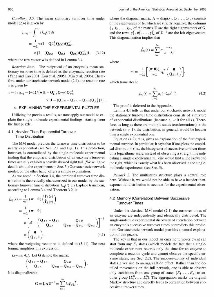
966 Journal of the American Statistical Association, September 2008
Corollary 3.5. The mean stationary turnover time undermodel (2.4) is given by
μeq =∫ ∞
0tfeq(t) dt
= 1
w1w(I − Q−1
CAQCC)Q−1BC
× [I − (QBB − QBA − QBC)Q−1AB ]1, (3.12)
where the row vector w is defined in Lemma 3.4.
Reaction Rate. The reciprocal of an enzyme’s mean sta-tionary turnover time is defined as the enzymatic reaction rate(Yang and Cao 2001; Kou et al. 2005a; Min et al. 2006). There-fore, under our stochastic network model (2.4), the reaction ratev is given by
v = 1/μeq = {w1}/{w(I − Q−1CAQCC)Q−1
BC
× [I − (QBB − QBA − QBC)Q−1AB ]1}
.
4. EXPLAINING THE EXPERIMENTAL PUZZLES
Utilizing the previous results, we now apply our model to ex-plain the single-molecule experimental findings, starting fromthe first puzzle.
4.1 Heavier-Than-Exponential TurnoverTime Distribution
The MM model predicts the turnover time distribution to benearly exponential (see Sec. 2.1 and Fig. 1). This prediction,however, is contradicted by the single-molecule experimentalfinding that the empirical distribution of an enzyme’s turnovertimes actually exhibits a heavily skewed right tail. (We will givedetails about the experiments in Sec. 5.) Our stochastic networkmodel, on the other hand, offers a simple explanation.
As we noted in Section 3.4, the empirical turnover time dis-tribution is theoretically characterized in our model by the sta-tionary turnover time distribution feq(t). Its Laplace transform,according to Lemma 3.4 and Theorem 3.2, is
feq(s) = 1
w1(w 0 )
(fA(s)
fB(s)
)
= 1
w1(w 0 )
×[sI −
(QAA − QAB QAB
QBA QBB − QBA − QBC
)]−1
×(
0QBC1
), (4.1)
where the weighting vector w is defined in (3.11). The nextlemma simplifies this expression.
Lemma 4.1. Let G denote the matrix(QAA − QAB QAB
QBA QBB − QBA − QBC
).
It is diagonalizable:
G = U�U−1 =2n∑i=1
λiξ iηTi ,
where the diagonal matrix � = diag(λ1, λ2, . . . , λ2n) consistsof the eigenvalues of G, which are strictly negative, the columnsξ1, ξ2, . . . , ξ2n of the matrix U are the right eigenvectors of G,and the rows ηT
1 ,ηT2 , . . . ,ηT
2n of U−1 are the left eigenvectors.This diagonalization implies that
feq(s) =2n∑i=1
σi
−λi
s − λi
,
where
σi = 1
−λi
[(w 0)ξ i
w1ηT
i
(0
QBC1
)],
which translates to
feq(t) =2n∑i=1
σi(−λieλi t ). (4.2)
The proof is deferred to the Appendix.Lemma 4.1 tells us that under our stochastic network model
the stationary turnover time distribution consists of a mixtureof exponential distributions (because λi < 0 for all i). There-fore, as long as there are multiple states (conformations) in thenetwork (n > 1), the distribution, in general, would be heavierthan a single exponential one.
Equation (4.2), thus, gives an explanation of the first experi-mental surprise. In particular, it says that if one plots the empiri-cal distribution (i.e., the histogram) of successive turnover timeson a logarithmic scale, instead of observing a straight line indi-cating a single-exponential tail, one would find a line skewed tothe right, which is exactly what has been observed in the single-molecule experiments (see Sec. 5).
Remark 2. The multistates structure plays a central rolehere. Without it, we would not be able to have a heavier-than-exponential distribution to account for the experimental obser-vation.
4.2 Memory (Correlation) Between SuccessiveTurnover Times
Under the classical MM model (2.1) the turnover times ofan enzyme are independently and identically distributed. Thesingle-molecule experimental discovery of correlation betweenan enzyme’s successive turnover times contradicts this predic-tion. Our stochastic network model provides a natural explana-tion of this puzzle.
The key is that in our model an enzyme turnover event canstart from any Ei states (which models the fact that a single-molecule experiment records only the time for an enzyme tocomplete a reaction cycle and cannot observe the specific en-zyme states; see Sec. 2.2). The unobservability of individualstates gives rise to an aggregation effect: Rather than the de-tailed movements on the full network, one is able to observeonly transitions from one group of states {E1, . . . ,En} to an-other group {E0
1, . . . ,E0n}. The aggregation masks the original
Markov structure and directly leads to correlation between suc-cessive turnover times.
Kou: Stochastic Networks in Nanoscale Biophysics 967
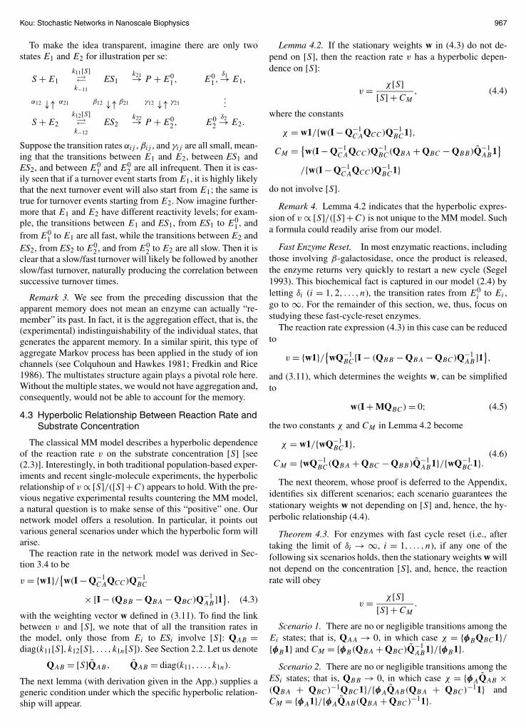
To make the idea transparent, imagine there are only twostates E1 and E2 for illustration per se:
S + E1
k11[S]�k−11
ES1k21→ P + E0
1, E01,
δ1→ E1,
α12 ↓↑ α21 β12 ↓↑ β21 γ12 ↓↑ γ21...
S + E2
k12[S]�k−12
ES2k22→ P + E0
2, E02
δ2→ E2.
Suppose the transition rates αij , βij , and γij are all small, mean-ing that the transitions between E1 and E2, between ES1 andES2, and between E0
1 and E02 are all infrequent. Then it is eas-
ily seen that if a turnover event starts from E1, it is highly likelythat the next turnover event will also start from E1; the same istrue for turnover events starting from E2. Now imagine further-more that E1 and E2 have different reactivity levels; for exam-ple, the transitions between E1 and ES1, from ES1 to E0
1 , andfrom E0
1 to E1 are all fast, while the transitions between E2 andES2, from ES2 to E0
2 , and from E02 to E2 are all slow. Then it is
clear that a slow/fast turnover will likely be followed by anotherslow/fast turnover, naturally producing the correlation betweensuccessive turnover times.
Remark 3. We see from the preceding discussion that theapparent memory does not mean an enzyme can actually “re-member” its past. In fact, it is the aggregation effect, that is, the(experimental) indistinguishability of the individual states, thatgenerates the apparent memory. In a similar spirit, this type ofaggregate Markov process has been applied in the study of ionchannels (see Colquhoun and Hawkes 1981; Fredkin and Rice1986). The multistates structure again plays a pivotal role here.Without the multiple states, we would not have aggregation and,consequently, would not be able to account for the memory.
4.3 Hyperbolic Relationship Between Reaction Rate andSubstrate Concentration
The classical MM model describes a hyperbolic dependenceof the reaction rate v on the substrate concentration [S] [see(2.3)]. Interestingly, in both traditional population-based exper-iments and recent single-molecule experiments, the hyperbolicrelationship of v ∝ [S]/([S]+C) appears to hold. With the pre-vious negative experimental results countering the MM model,a natural question is to make sense of this “positive” one. Ournetwork model offers a resolution. In particular, it points outvarious general scenarios under which the hyperbolic form willarise.
The reaction rate in the network model was derived in Sec-tion 3.4 to be
v = {w1}/{w(I − Q−1CAQCC)Q−1
BC
× [I − (QBB − QBA − QBC)Q−1AB ]1}
, (4.3)
with the weighting vector w defined in (3.11). To find the linkbetween v and [S], we note that of all the transition rates inthe model, only those from Ei to ESi involve [S]: QAB =diag(k11[S], k12[S], . . . , k1n[S]). See Section 2.2. Let us denote
QAB = [S]QAB, QAB = diag(k11, . . . , k1n).
The next lemma (with derivation given in the App.) supplies ageneric condition under which the specific hyperbolic relation-ship will appear.
Lemma 4.2. If the stationary weights w in (4.3) do not de-pend on [S], then the reaction rate v has a hyperbolic depen-dence on [S]:
v = χ[S][S] + CM
, (4.4)
where the constants
χ = w1/{w(I − Q−1CAQCC)Q−1
BC1},CM = {
w(I − Q−1CAQCC)Q−1
BC(QBA + QBC − QBB)Q−1AB1
}/{w(I − Q−1
CAQCC)Q−1BC1}
do not involve [S].Remark 4. Lemma 4.2 indicates that the hyperbolic expres-
sion of v ∝ [S]/([S]+C) is not unique to the MM model. Sucha formula could readily arise from our model.
Fast Enzyme Reset. In most enzymatic reactions, includingthose involving β-galactosidase, once the product is released,the enzyme returns very quickly to restart a new cycle (Segel1993). This biochemical fact is captured in our model (2.4) byletting δi (i = 1,2, . . . , n), the transition rates from E0
i to Ei ,go to ∞. For the remainder of this section, we, thus, focus onstudying these fast-cycle-reset enzymes.
The reaction rate expression (4.3) in this case can be reducedto
v = {w1}/{wQ−1BC[I − (QBB − QBA − QBC)Q−1
AB ]1},
and (3.11), which determines the weights w, can be simplifiedto
w(I + MQBC) = 0; (4.5)
the two constants χ and CM in Lemma 4.2 become
χ = w1/{wQ−1BC1},
(4.6)CM = {wQ−1
BC(QBA + QBC − QBB)Q−1AB1}/{wQ−1
BC1}.The next theorem, whose proof is deferred to the Appendix,
identifies six different scenarios; each scenario guarantees thestationary weights w not depending on [S] and, hence, the hy-perbolic relationship (4.4).
Theorem 4.3. For enzymes with fast cycle reset (i.e., aftertaking the limit of δi → ∞, i = 1, . . . , n), if any one of thefollowing six scenarios holds, then the stationary weights w willnot depend on the concentration [S], and, hence, the reactionrate will obey
v = χ[S][S] + CM
.
Scenario 1. There are no or negligible transitions among theEi states; that is, QAA → 0, in which case χ = {φBQBC1}/{φB1} and CM = {φB(QBA + QBC)Q−1
AB1}/{φB1}.Scenario 2. There are no or negligible transitions among the
ESi states; that is, QBB → 0, in which case χ = {φAQAB ×(QBA + QBC)−1QBC1}/{φAQAB(QBA + QBC)−11} andCM = {φA1}/{φAQAB(QBA + QBC)−11}.

968 Journal of the American Statistical Association, September 2008
Scenario 3. The transitions among the Ei states are muchfaster than the others; that is, QAA = κQAA, and the scale κ ismuch larger than the other transition rates: κ → ∞. In this caseχ = {φAQAB(QBB −QBA −QBC)−1QBC1}/{φAQAB(QBB −QBA − QBC)−11} and CM = {φA1}/{φAQAB(QBA + QBC −QBB)−11}.
Scenario 4. The transitions among the ESi states are muchfaster than the others; that is, QBB = κQBB , and the scaleκ is much larger than the other transition rates: κ → ∞.In this case χ = {φBQBC1}/{φB1} and CM = {φB(QBA +QBC)Q−1
AB1}/{φB1}.Scenario 5. The transition rate from ESi to Ei is much
larger than the rate from ESi to E0i ; that is, k−1i k2i for
i = 1,2, . . . , n. In this case χ = {φBQBC1}/{φB1} and CM ={φB(QBA + QBC)Q−1
AB1}/{φB1}.Scenario 6. For all the ESi states, the ratios between the for-
ward and backward transition rates are the same: k21/k−11 =k22/k−12 = · · · = k2i/k−1i = · · · = k2n/k−1n. In this case χ ={φBQBC1}/{φB1} and CM = {φB(QBA+QBC)Q−1
AB1}/{φB1}.Note that the row vectors φA and φB referred to previously
are defined by (3.3) and (3.4).
The six scenarios in Theorem 4.3, each covering a large classof enzymes, have their biochemical implications. Scenarios1 and 2 correspond to the so-called slow fluctuating enzymes,those whose conformations fluctuate/interconvert slowly; Sce-narios 3 and 4 correspond to fast fluctuating enzymes, thosehaving fast conformational fluctuations; Scenario 5 corre-sponds to the so-called primitive enzymes, those whose dis-sociation rate is much larger than their catalytic rate (Alberyand Knowles 1976; Min et al. 2006); Scenario 6 correspondsto conformational-equilibrium enzymes, those possessing thechemical property that the energy–barrier difference betweentheir dissociation and catalysis is invariant across conforma-tions (Min et al. 2006).
By pointing out various general cases under which the hy-perbolic relationship between v and [S] arises from our model,Theorem 4.3 and Lemma 4.2 provide an explanation of the thirdexperimental puzzle: Although the MM model gives the de-scription of v ∝ [S]/([S] + C), observing such a relationshipin experiments by no means implies that the MM model is theunderlying mechanism because the MM model is only one ofmany that display such a relationship—the discovery of mem-ory and heavier-than-exponential distribution of the turnovertimes points to the opposite direction. This understanding helpsreconcile the long-held belief in the MM model with the recentsingle-molecule experimental surprises. For decades, numeroustraditional experiments on different enzymes yielded the v ∝[S]/([S] + C) relationship; because of this, they were viewedas strong evidence for the MM model. Now we know that thesetraditional experimental outcomes can be better viewed as evi-dence for our more general stochastic network model.
5. FROM THEORY TO EXPERIMENTAL DATA
A recent single-molecule experiment (English et al. 2006)conducted by the Xie group at Harvard University (Departmentof Chemistry and Chemical Biology) studied β-galactosidase
(β-gal), an essential enzyme in the human body that catalyzesthe breakdown of the sugar lactose (Jacobson et al. 1994; Dor-land 2003). In the experiment a single β-gal molecule is immo-bilized (to a bead), which allows its enzymatic turnovers to becontinuously monitored under a fluorescence microscope. Todetect the individual turnovers, careful design and special treat-ment were carried out so that once the experimental system wasplaced under a laser beam the reaction product and only the re-action product was fluorescent. This setting ensures that as theβ-gal enzyme catalyzes one substrate molecule after another,a strong fluorescence signal is emitted and detected only whena product is released, that is, only when the enzyme reachesthe E0
i + P stage [see (2.1) and (2.4) for diagrams]. Recordingthe fluorescence signals over time thus enables the experimentaldetermination of individual turnovers.
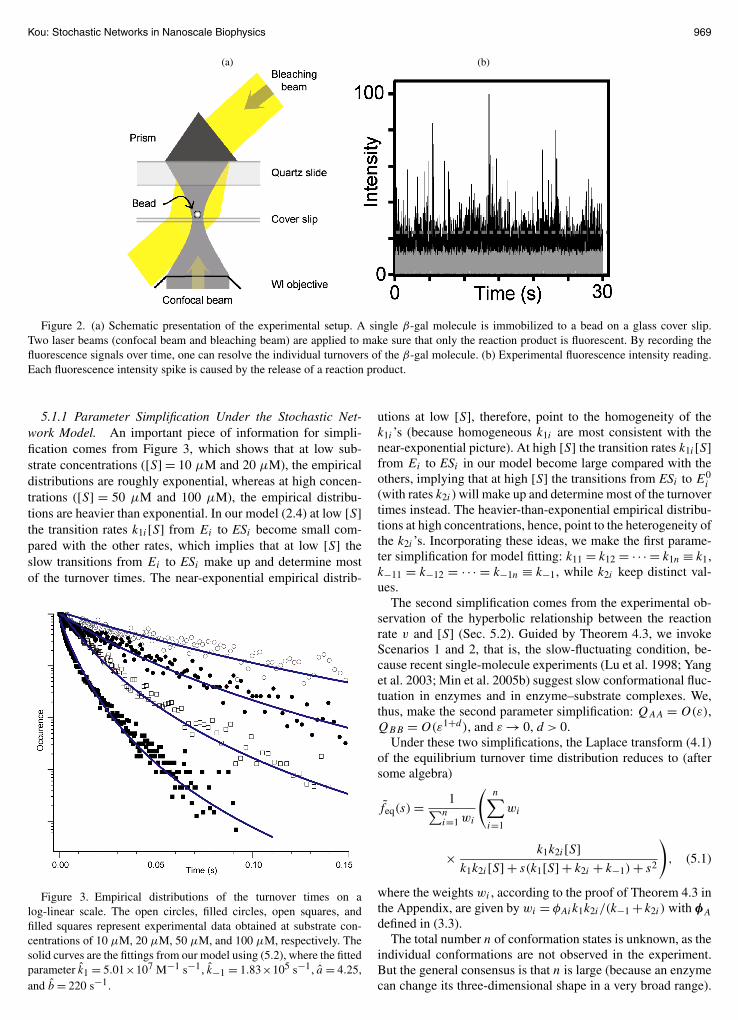
Figure 2(a) presents a schematic picture of the experimentalsetup. Figure 2(b) shows a typical fluorescence intensity read-ing from the experiment: Each vertical bar is a fluorescence in-tensity spike generated by the release of one reaction product.
Because β-gal is a fast-reset enzyme (Sec. 4.3), the timelag between two adjacent fluorescence spikes is the enzymaticturnover time. Thus, by moving along the time axis and tak-ing the time lag between every two consecutive fluorescencespikes [the vertical bars in Fig. 2(b)], one obtains the succes-sive turnover times of the β-gal molecule (in this way the rawexperimental record was translated into numerical datasets).
To investigate how the substrate concentration [S] affects theturnover times, the experiment was repeated at different levelsof [S]; throughout each repetition the substrate concentration[S] is held at a fixed level.
5.1 Experimental Turnover Time Distributions
The empirical distributions of the experimental turnovertimes obtained at four substrate concentrations [S] = 10 μM,20 μM, 50 μM, and 100 μM (micromolar) are plotted in Fig-ure 3 on a log-linear scale (open circles, filled circles, opensquares, and filled squares correspond to the four substrate con-centrations, respectively). Rather than following straight lineson the logarithmic scale as the MM model predicts, the empir-ical distributions have curved tails at high substrate concentra-tions.
Applying Pearson’s chi-squared test, we assess the good-ness of fit of the MM model. Using 10 equally spaced bins(along the x axis), we calculate the Pearson chi-squared sta-tistic
∑i (Oi − Ei)
2/Ei , where the expected bin counts Ei arecalculated from (2.2). For the experimental data at [S] = 50 μMand 100 μM, the p values are both less than 1%.
A careful reader might ask: Why were the curved tails not ob-served in the classical population-based ensemble experiments?The answer is that, although, in principle, the classical experi-ments should also observe these curved tails, in practice, with-out the capability to track individual enzymes, the classical ex-periments can only record the fast reaction turnovers, and theslow turnovers that constitute the curved tails are entirely miss-ing.
Now, as a check of our stochastic network model, we fit it tothe empirical turnover time distributions. To do so, we note thatthe model parameters need to be constrained/simplified becauseso far there are too many.
Kou: Stochastic Networks in Nanoscale Biophysics 969
(a) (b)
Figure 2. (a) Schematic presentation of the experimental setup. A single β-gal molecule is immobilized to a bead on a glass cover slip.Two laser beams (confocal beam and bleaching beam) are applied to make sure that only the reaction product is fluorescent. By recording thefluorescence signals over time, one can resolve the individual turnovers of the β-gal molecule. (b) Experimental fluorescence intensity reading.Each fluorescence intensity spike is caused by the release of a reaction product.
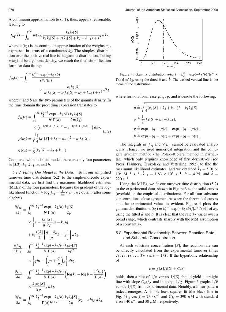
5.1.1 Parameter Simplification Under the Stochastic Net-work Model. An important piece of information for simpli-fication comes from Figure 3, which shows that at low sub-strate concentrations ([S] = 10 μM and 20 μM), the empiricaldistributions are roughly exponential, whereas at high concen-trations ([S] = 50 μM and 100 μM), the empirical distribu-tions are heavier than exponential. In our model (2.4) at low [S]the transition rates k1i[S] from Ei to ESi become small com-pared with the other rates, which implies that at low [S] theslow transitions from Ei to ESi make up and determine mostof the turnover times. The near-exponential empirical distrib-
Figure 3. Empirical distributions of the turnover times on alog-linear scale. The open circles, filled circles, open squares, andfilled squares represent experimental data obtained at substrate con-centrations of 10 μM, 20 μM, 50 μM, and 100 μM, respectively. Thesolid curves are the fittings from our model using (5.2), where the fittedparameter k1 = 5.01×10⁷ M−1 s−1, k−1 = 1.83×10⁵ s−1, a = 4.25,and b = 220 s−1.
utions at low [S], therefore, point to the homogeneity of thek1i ’s (because homogeneous k1i are most consistent with thenear-exponential picture). At high [S] the transition rates k1i[S]from Ei to ESi in our model become large compared with theothers, implying that at high [S] the transitions from ESi to E0
i(with rates k2i ) will make up and determine most of the turnovertimes instead. The heavier-than-exponential empirical distribu-tions at high concentrations, hence, point to the heterogeneity ofthe k2i ’s. Incorporating these ideas, we make the first parame-ter simplification for model fitting: k11 = k12 = · · · = k1n ≡ k1,k−11 = k−12 = · · · = k−1n ≡ k−1, while k2i keep distinct val-ues.
The second simplification comes from the experimental ob-servation of the hyperbolic relationship between the reactionrate v and [S] (Sec. 5.2). Guided by Theorem 4.3, we invokeScenarios 1 and 2, that is, the slow-fluctuating condition, be-cause recent single-molecule experiments (Lu et al. 1998; Yanget al. 2003; Min et al. 2005b) suggest slow conformational fluc-tuation in enzymes and in enzyme–substrate complexes. We,thus, make the second parameter simplification: QAA = O(ε),QBB = O(ε1+d), and ε → 0, d > 0.
Under these two simplifications, the Laplace transform (4.1)of the equilibrium turnover time distribution reduces to (aftersome algebra)
feq(s) = 1∑ni=1 wi
(n∑
i=1
wi
× k1k2i[S]k1k2i[S] + s(k1[S] + k2i + k−1) + s2
), (5.1)
where the weights wi , according to the proof of Theorem 4.3 inthe Appendix, are given by wi = φAik1k2i/(k−1 + k2i ) with φA
defined in (3.3).The total number n of conformation states is unknown, as the
individual conformations are not observed in the experiment.But the general consensus is that n is large (because an enzymecan change its three-dimensional shape in a very broad range).
970 Journal of the American Statistical Association, September 2008
A continuum approximation to (5.1), thus, appears reasonable,leading to
feq(s) =∫ ∞
0w(k2)
k1k2[S]k1k2[S] + s(k1[S] + k2 + k−1) + s2
dk2,
where w(k2) is the continuum approximation of the weights wi ,expressed in terms of a continuous k2. The simplest distribu-tion over the positive real line is the gamma distribution. Takingw(k2) to be a gamma density, we reach the final simplificationform for data fitting:
feq(s) =∫ ∞
0
ka−12 exp(−k2/b)
ba (a)
× k1k2[S]k1k2[S] + s(k1[S] + k2 + k−1) + s2
dk2,
where a and b are the two parameters of the gamma density. Inthe time domain the preceding expression translates to
feq(t) =∫ ∞
0
ka−12 exp(−k2/b)
ba (a)
k1k2[S]2p(k2)
× (e−[q(k2)−p(k2)]t − e−[q(k2)+p(k2)]t)dk2,
(5.2)
p(k2) =√
1
4(k1[S] + k2 + k−1)2 − k1k2[S],
q(k2) = 1
2(k1[S] + k2 + k−1).
Compared with the initial model, there are only four parametersin (5.2): k1, k−1, a, and b.
5.1.2 Fitting Our Model to the Data. To fit our simplifiedturnover time distribution (5.2) to the single-molecule exper-imental data, we first find the maximum likelihood estimates(MLEs) of the four parameters. Because the gradient of the log-likelihood function ∇ logfeq = 1
feq∇feq, we obtain (after some
algebra)
∂feq
∂k1=
∫ ∞
0
ka−12 exp(−k2/b)
ba (a)
k2[S]2p
×{g − k1
p
[S]2p
(q − k2)g
+ k1t[S]
2
{q − k2
ph − g
}}dk2,
∂feq
∂k−1=
∫ ∞
0
ka−12 exp(−k2/b)
ba (a)
k1k2[S]4p2
×{qht −
(pt + q
p
)g
}dk2,
∂feq
∂a=
∫ ∞
0
ka−12 exp(−k2/b)
ba (a)
(logk2 − logb − ′(a)
(a)
)
× k1k2[S]2p
g dk2,
∂feq
∂b=
∫ ∞
0
ka−12 exp(−k2/b)
(a)ba+2
k1k2[S]2p
(k2 − ab)g dk2,
Figure 4. Gamma distribution w(k2) = ka−12 exp(−k2/b)/[ba ×
(a)] of k2, using the fitted a and b. The dashed vertical line is themean of the distribution.
where for notational ease p, q , g, and h denote the following:
p �√
1
4(k1[S] + k2 + k−1)2 − k1k2[S],
q � 1
2(k1[S] + k2 + k−1),
g � exp(−(q − p)t) − exp(−(q + p)t),
h � exp(−(q − p)t) + exp(−(q + p)t).
The integrals in feq and ∇feq cannot be evaluated analyt-ically. Hence, we used numerical integration and the conju-gate gradient method (the Polak–Ribiere method in particu-lar), which only requires knowledge of first derivatives (seePress, Flannery, Teukolsky, and Vetterling 1992), to find themaximum likelihood estimates, and we obtained k1 = 5.01 ×10⁷ M−1 s−1, k−1 = 1.83 × 10⁵ s−1, a = 4.25, and b =220 s−1.
Using the MLEs, we fit our turnover time distribution (5.2)to the experimental data, shown in Figure 3 as the solid curves(overlaid on the empirical distributions). For all four substrateconcentrations, close agreement between the theoretical curvesand the experimental values is evident. Figure 4 plots thegamma distribution w(k2) = ka−1
2 exp(−k2/b)/[ba (a)] of k2,using the fitted a and b. It is clear that the rate k2 varies over abroad range, which contrasts sharply with the MM assumptionof a constant k2.
5.2 Experimental Relationship Between Reaction Rateand Substrate Concentration
At each substrate concentration [S], the reaction rate canbe directly calculated from the experimental turnover timesT1, T2, T3, . . . , TN via v = 1/T . If the hyperbolic relationshipof
v = χ[S]/([S] + CM)
holds, then a plot of 1/v versus 1/[S] should yield a straightline with slope CM/χ and intercept 1/χ . Figure 5 graphs 1/v
versus 1/[S] from experimental data. Notably, a linear patternindeed emerges. A simple least squares fit (the black line inFig. 5) gives χ = 730 s−1 and CM = 390 μM with standarderrors 40 s−1 and 30 μM, respectively.

Kou: Stochastic Networks in Nanoscale Biophysics 971
Figure 5. Plot of 1/v versus 1/[S] from the experimental data. Thereaction rate v at each point is calculated from the experimental data atthe corresponding substrate concentration. The black line is the leastsquares fit with χ = 730 ± 80 s−1 and CM = 390 ± 60 μM.
As a consistency check of our model, we compute from for-mula (5.2) that
μeq =∫ ∞
0tfeq(t) dt
=∫ ∞
0
ka−12 exp(−k2/b)
ba (a)
k1[S] + k2 + k−1
k1k2[S] dk2
= [S] + (k−1 + b(a − 1))/k1
b(a − 1)[S] ,
which gives
v = 1
μeq= b(a − 1)[S]
[S] + (k−1 + b(a − 1))/k1≡ χ ′[S]
[S] + C′M
.
Plugging in the MLEs of Figure 3, we note that χ ′ = b(a−1) =715 s−1 and C′
M = (k−1 + b(a − 1))/k1 = 380 μM agreewell with the least squares nonparametric estimates of χ =730 ± 80 s−1 and CM = 390 ± 60 μM given previously (meanplus/minus twice the standard error).
5.3 Experimental Autocorrelation of Turnover Times
From the experimental successive turnover times T1, T2,
T3, . . . , TN , one can calculate their empirical autocovariance
Cov(m) = 1
N − m
∑i
(Ti − T )(Ti+m − T ).
Figure 6 shows the empirical autocorrelation function, plottingthe normalized Cov(m) against mT for m = 1,2, . . . at a rep-resentative substrate concentration [S] = 100 μM. Instead of aflat horizontal line at 0 as the MM model would predict, a clearmemory effect is seen in Figure 6. The experimental data atother substrate concentrations showed a similar correlation pic-ture. The evident memory indicates strongly that the classicalMM missed important aspects of real enzymatic reactions andthat models like ours that can account for the memory are nec-essary.
6. DISCUSSION
In this article we introduce a stochastic network model toexplain the experimental puzzles arising from single-moleculestudies of enzymatic reactions. The use of the multiple states
Figure 6. Turnover time autocorrelation function. Cov(m) is plot-ted against mT from the experimental data at substrate concentration[S] = 100 μM.
(to capture the enzyme’s conformational fluctuation) plays afundamental role in the model’s success. We conduct a de-tailed study of the model (such as analyzing the first-passage-time distributions). Using the analytical results, we show thatthe model explains (a) the heavier-than-exponential empiricalturnover time distributions, (b) the memory effect of turnovertimes, and (c) the observed hyperbolic relationship between en-zymatic reaction rate and substrate concentration.
The model has three additional appealing features. (1) It of-fers analytical tractability as the results in Sections 3 and 4 illus-trate. (2) The theoretical results from the model agree well withthe experimental data (as seen in Sec. 5). (3) The model has asolid biological/chemical underpinning—each component andparameter in the model has its biological/chemical meaning.
Some problems remain open for future exploration.
1. When we estimated the model parameters in Section 5.1,we first calculated the log-likelihood by adding up the log-density contribution from each observed turnover timeand then maximized it. Because this calculation essen-tially ignores the correlation of the turnover times, it is, infact, a quasi-likelihood method (Heyde 1997). Althoughergodicity ensures the consistency, a theoretical investi-gation of its efficiency remains open.
2. We simultaneously fit the turnover time distributions atmultiple concentrations. Extending the fitting to the auto-correlation functions is open for further study.
3. When we fit our model to the experimental data, we usedthe continuum limit by letting the number of states n goto ∞ and then assumed a gamma distribution. Althoughthis simple approach fits the experimental data well, itremains to be seen if the continuum limit and gammadistribution can be derived directly from a more biolog-ical/biophysical microscopic angle. Such study will pro-vide an interesting connection between statistics and bio-physics by giving the statistical assumptions a biologicalunderpinning; it will, furthermore, lead to not only poten-tially better approximation schemes, but also new insightinto the biological nature of an enzyme’s conformation

972 Journal of the American Statistical Association, September 2008
fluctuation (e.g., the potential mean field in the conforma-tion space).
4. In fitting the data we applied the slow-fluctuating-enzymecondition, because it appeared most natural. A problemfor future study is to explore the other scenarios of Theo-rem 4.3, investigate how to constrain the model parame-ters under these scenarios, and compare their fittings tothe data. Such investigation will help pin down the rolethat conformational fluctuation plays in enzymatic reac-tions and can potentially guide the design of new exper-iments to elucidate the underlying microscopic biophysi-cal picture.
The new field of nanoscale (single-molecule) biophysics hasattracted much attention from biologists, chemists, and physi-cists, as it holds promise for new scientific discoveries. It alsopresents many interesting problems for statisticians because ofthe stochastic nature of the nanometer world. Our stochasticnetwork model for single-molecule enzymatic reaction exem-plifies only one instance of the numerous and growing researchopportunities in nanoscale biophysics. We hope that this articlewill generate further interest in applying modern statistical andprobabilistic methodology to interesting biophysical and scien-tific problems.
APPENDIX: PROOFS
Proof of Proposition 2.1
To obtain the turnover time distribution under the MM model, letTE and TES denote the first passage times to reach E0 from states E
and ES, respectively, and let fE(t) and fES(t) be their correspondingdensity functions. The routing map (2.1) immediately gives
TEd= Ek1[S] + TES, (A.1)
where the random variables on the right side are independent of eachother, and throughout this proof, Eρ denotes an exponential randomvariable with rate ρ. Next, noting that one can go either forward orbackward from state ES with the two directions characterized by twoexponential random variables Ek2 and Ek−1 , we have
fES(t) dt = P(TES ∈ (t, t + dt))
= P(TES ∈ (t, t + dt), Ek2 < Ek−1
)+ P
(TES ∈ (t, t + dt), Ek2 > Ek−1
)= P
(Ek2 ∈ (t, t + dt), Ek2 < Ek−1
)+ P
(Ek−1 + TE ∈ (t, t + dt), Ek2 > Ek−1
)= k2e−(k2+k−1)t dt
+(∫ t
0fE(t − z)k−1e−(k2+k−1)z dz
)dt
+ o(dt). (A.2)
In the Laplace space (A.1) and (A.2) become
fE(s) = k1[S]k1[S] + s
fES(s),
fES(s) = k2
k2 + k−1 + s+ k−1
k2 + k−1 + sfE(s),
where fE(s) and fES(s) are the Laplace transforms of fE(t) andfES(t), respectively [i.e., fJ (s) = ∫ ∞
0 e−st fJ (t) dt , J = E or ES].
Solving them, we obtain
fE(s) = k1k2[S]k1k2[S] + s(k1[S] + k2 + k−1) + s2
,
and correspondingly the density function of the turnover time is
fE(t) = k1k2[S](e−(q−p)t − e−(q+p)t)/(2p),
where p =√
(k1[S] + k2 + k−1)2/4 − k1k2[S] and q = (k1[S]+k2 +k−1)/2.
Proof of Lemma 3.1
Let Yn denote the embedded Markov chain associated with X(t)
[i.e., Yn is the discrete-time Markov chain corresponding to the jumpsof X(t)]. It is straightforward to check that Yn is irreducible andaperiodic and is, thus, positive recurrent. This guarantees that (seeKijima 1997) (1) X(t) is ergodic, (2) the stationary distribution ofX(t) exists and is unique, and (3) the stationary distribution satisfies(πA,πB,πC)Q = 0. The definition (2.5) of Q then gives
(πA,πB,πC)
×(QAA − QAB QAB 0
QBA QBB − (QBA + QBC) QBC
QCA 0 QCC − QCA
)= 0,
which implies that
(πA,πB)
(QAA − QAB QAB
QBA QBB − (QBA + QBC)
)
+ πC (QCA 0 ) = 0, (A.3)
πBQBC + πC(QCC − QCA) = 0. (A.4)
From (A.3) we have
(πA,πB) = −πC (QCA 0 )
×(
QAA − QAB QAB
QBA QBB − (QBA + QBC)
)−1.
The formula for block-matrix inversion provides
(QAA − QAB QAB
QBA QBB − (QBA + QBC)
)−1=
(L MN R
), (A.5)
where
L = [QAA − QAB − QAB(QBB − QBA − QBC)−1QBA]−1,
M = [QBB − QBC − (QBB − QBA − QBC)Q−1AB
QAA]−1,(A.6)
N = [QAA − (QAA − QAB)Q−1BA
(QBB − QBC)]−1,
R = [QBB − QBA − QBC − QBA(QAA − QAB)−1QAB ]−1.
Therefore,
(πA,πB) = −πC (QCA 0 )
(L MN R
)
= −(πCQCAL, πCQCAM), (A.7)
Substituting (A.7) into (A.4), we have the final equation for πC :πC(QCC − QCA − QCAMQBC) = 0.

Kou: Stochastic Networks in Nanoscale Biophysics 973
Proof of Theorem 3.2
Consider a Markov chain Z(t) modified from X(t) by making{E0
1 , . . . ,E0n} absorbing (see Keilson 1979; Kijima 1997). It has tran-
sition matrix
Qz =(QAA − QAB QAB 0
QBA QBB − (QBA + QBC) QBC
0 0 0
).
The first passage time to {E01 , . . . ,E0
n} for X(t) is the same as theabsorbing time of Z(t). Applying a first-step analysis and noting thereis no direct transition from Ei to E0
j, we have
P(TI ∈ (t, t + dt)) =∑
J∈{ES1,...,ESn}
∑K∈{E0
1 ,...,E0n}
PIJ (t)(Qz)JK dt
+ o(dt) for I = Ei or ESi ,
where PIJ (t) is Z(t)’s transition probability from state I to state J attime t ; in matrix form the equation can be written as
(fA(t)
fB(t)
)dt = P(t)
(0
QBC1
)dt + o(dt), (A.8)
where P(t) is the sub–transition matrix of Z(t) corresponding to thenonabsorbing states.
The full transition matrix of Z(t) is exp(Qzt), of which P(t) is theupper-left block. It is straightforward to verify from block-matrix cal-culation that
P(t) = exp
((QAA − QAB QAB
QBA QBB − (QBA + QBC)
)t
),
which (according to the basic properties of matrix exponential) hasLaplace transform
P(s) =∫ ∞
0exp(−st)P(t) dt
=[sI −
(QAA − QAB QAB
QBA QBB − QBA − QBC
)]−1.
Applying a Laplace transform on (A.8) and using the previous formulafor P(s), we finally obtain (3.9).
Proof of Corollary 3.3
Equation (3.9) gives
s
(fA(s)
fB(s)
)=
(QAA − QAB QAB
QBA QBB − (QBA + QBC)
)(fA(s)
fB(s)
)
+(
0QBC1
).
Taking the derivative with respect to s in the preceding expression andevaluating it at s = 0 yield
(μA
μB
)= −
( f′A
(0)
f′B
(0)
)
= −(
QAA − QAB QAB
QBA QBB − (QBA + QBC)
)−1 (11
),
which is simplified to (3.10) by the block-matrix inversion (A.5)and (A.6).
Proof of Lemma 3.4
Because a turnover event begins right after the enzyme enters theEi (i = 1,2, . . . , n) state from the E0
istate (see Sec. 2.2), it follows
that the stationary probability w(Ei) is proportional to the probabil-ity flux from E0
ito Ei , that is, the expected number of transitions
from E0i
to Ei per unit time. The latter is given by π(E0i)δi according
to Levy’s formula (see Serfozo 1999). Therefore, the weight vector(w(Ei), . . . ,w(En)) ∝ w = πCQCA. According to Lemma 3.1, πC
satisfies (3.6), which implies immediately that w must satisfy (3.11).
Proof of Corollary 3.5
From Lemma 3.4 we know μeq = (wμA)/(w1), which by Corol-lary 3.3 is μeq = −[w(L + M)1]/(w1). Next, it is straightfor-ward to verify from the definition of L and M in Lemma 3.1that L = −M(QBB − QBA − QBC)Q−1
AB, which implies L + M =
−M[(QBB − QBA − QBC)Q−1AB
− I]. It, thus, follows that
μeq = 1
w1wM[(QBB − QBA − QBC)Q−1
AB− I]1.
The definition (3.11) of w tells us that wM = w(Q−1CA
QCC − I)Q−1BC
.Plugging it into the preceding expression yields (3.12).
Proof of Lemma 4.1
The detailed balance condition (3.2) tells us that(
�A 00 �B
)G is
symmetric, because �A, �B , QAB , QBA, and QBC are all diago-
nal matrices. Hence, the matrix(
�A 00 �B
)1/2G
(�A 00 �B
)−1/2is also
symmetric and, thus, admits a spectral decomposition. Consequently,G is diagonalizable: G = U�U−1 = ∑2n
i=1 λiξ iηTi
, where λi are the
eigenvalues of G, and ξ i and ηTi
are the corresponding right and lefteigenvectors, respectively. This implies that
(sI − G)−1 =2n∑i=1
1
s − λiξ iη
Ti ,
which means that feq(s) can be re-expressed as
feq(s) =2n∑i=1
1
s − λi
[(w 0)ξ i
w1ηTi
(0
QBC1
)].
The matrix G satisfies
G1 =(
QAA − QAB QAB
QBA QBB − QBA − QBC
)(11
)
= −(
0QBC1
). (A.9)
Because the diagonal elements of QBC are all positive, (A.9) impliesthat G is a lossy generator (see Keilson 1979; Kijima 1997), and,hence, all its eigenvalues λi are strictly negative. Thus, we can rewrite
feq(s) =2n∑i=1
σi−λi
s − λi,
σi = 1
−λi
[(w 0)ξ i
w1ηTi
(0
QBC1
)],
which translates to feq(t) = ∑2ni=1 σi(−λie
λi t ).
974 Journal of the American Statistical Association, September 2008
Proof of Lemma 4.2
With w not depending on [S], direct calculation from (4.3) yields
v = {w1}/{
w(I − Q−1CA
QCC)Q−1BC
×{
I − 1
[S] (QBB − QBA − QBC)Q−1AB
}1}
= (w1/{w(I − Q−1
CAQCC)Q−1
BC1}[S])/([S] − {w(I − Q−1
CAQCC)Q−1
BC(QBB − QBA − QBC)Q−1
AB1}
/{w(I − Q−1CA
QCC)Q−1BC
1}),which is (4.4).
Proof of Theorem 4.3
We have seen that for enzymes with fast cycle reset the equi-librium weights w are determined by (4.5), which is equivalent tow(I + Q−1
BCM−1) = 0.
The definition (3.8) of M gives
I + Q−1BC
M−1
= Q−1BC
QBB − Q−1BC
(QBB − QBA − QBC)Q−1AB
QAA
= Q−1BC
QBB − Q−1BC
(QBB − QBA − QBC)Q−1AB
QAA/[S].Consider Scenario 1 now. This scenario (QAA → 0) implies that
I + Q−1BC
M−1 → Q−1BC
QBB . So in this case w is the nonzero solu-
tion of wQ−1BC
QBB = 0. We know from Section 3.1 that φBQBB = 0.Therefore, w = φBQBC , which does not depend on [S]. Accordingto Lemma 4.2 and (4.6), we then have v = χ [S]/([S] + CM), whereχ = φBQBC1/{φB1} and CM = {φB(QBA + QBC)Q−1
AB1}/{φB1}.
Consider Scenario 2 next. This scenario (QBB → 0) impliesthat I + Q−1
BCM−1 → Q−1
BC(QBA + QBC)Q−1
ABQAA/[S]. So w is
the solution of wQ−1BC
(QBA + QBC)Q−1AB
QAA = 0. We know that
φAQAA = 0 from Section 3.1. Therefore, w = φAQAB(QBA +QBC)−1QBC , which does not depend on [S]. Lemma 4.2 and (4.6)then tell us that v = χ [S]/([S] + CM), where χ = {φAQAB(QBA +QBC)−1QBC1}/{φAQAB(QBA + QBC)−11} and CM = {φA1}/{φAQAB(QBA + QBC)−11}.
Consider Scenario 3. Under this scenario (QAA = κQAA withthe scale κ → ∞), (I + Q−1
BCM−1)/κ → −Q−1
BC(QBB − QBA −
QBC)Q−1AB
QAA/[S]. Hence, w is the solution of wQ−1BC
(QBB −QBA − QBC)Q−1
ABQAA = 0. Because φAQAA = 0, it follows that
w = φAQAB(QBB − QBA − QBC)−1QBC , which does not dependon [S]. Lemma 4.2 and (4.6) then imply v = χ [S]/([S] + CM), whereχ = {φAQAB(QBB − QBA − QBC)−1QBC1}/{φAQAB(QBB −QBA − QBC)−11} and CM = −{φA1}/{φAQAB(QBB − QBA −QBC)−11}.
Consider Scenario 4. Under this scenario (QBB = κQBB with thescale κ → ∞), (I + Q−1
BCM−1)/κ → Q−1
BCQBB − Q−1
BCQBBQ−1
AB×
QAA/[S], which tells us that w is the solution of w(Q−1BC
QBB −Q−1
BCQBBQ−1
ABQAA/[S]) = 0. Because φBQBB = 0, it follows that
w = φBQBC , which does not depend on [S]. Lemma 4.2 and (4.6)then imply v = χ [S]/([S] + CM), where χ = φBQBC1/{φB1} andCM = −{φB(QBB − QBA − QBC)Q−1
AB1}/{φB1} ={φB(QBA +
QBC)Q−1AB
1}/{φB1}.Consider Scenario 5. This scenario (k−1i k2i ) implies that
QBA +QBC ≈ QBA, so I+Q−1BC
M−1 → Q−1BC
QBB −Q−1BC
(QBB −QBA)Q−1
ABQAA/[S]. Therefore, w is the solution of w{Q−1
BCQBB −
Q−1BC
(QBB − QBA)Q−1AB
QAA/[S]} = 0. Using the facts that φA ×
QAA = φBQBB = 0 and φAQAB [S] = φBQBA (see Sec. 3.1),we can verify that w = φBQBC is the solution, which does notdepend on [S]. We thus know from Lemma 4.2 and (4.6) thatv = χ [S]/([S] + CM), where χ = φBQBC1/{φB1} and CM ={φB(QBA + QBC)Q−1
AB1}/{φB1}.
Finally, consider Scenario 6. This scenario implies that QBC ∝QBA, say QBC = κQBA. So I + Q−1
BCM−1 = Q−1
BCQBB − Q−1
BC×
(QBB − (1 + κ)QBA)Q−1AB
QAA/[S]. Using the facts that φAQAA =φBQBB = 0 and φAQAB [S] = φBQBA, we can verify that w =φBQBC is the solution of w(I + Q−1
BCM−1) = 0. It does not de-
pend on [S]. It, thus, follows from Lemma 4.2 and (4.6) thatv = χ [S]/([S] + CM), where χ = φBQBC1/{φB1} and CM ={φB(QBA + QBC)Q−1
AB1}/{φB1}.
[Received January 2007. Revised May 2007.]
REFERENCES
Albery, W. J., and Knowles, J. R. (1976), “Free-Energy Profile for the ReactionCatalyzed by Triosephosphate Isomerase,” Biochemistry, 15, 5627–5631.
Asbury, C., Fehr, A., and Block, S. M. (2003), “Kinesin Moves by an Asym-metric Hand-Over-Hand Mechanism,” Science, 302, 2130–2134.
Atkins, P., and de Paula, J. (2002), Physical Chemistry (7th ed.), New York:W. H. Freeman.
Ball, K., Kurtz, T. G., Popovic, L., and Rempala, G. (2006), “AsymptoticAnalysis of Multiscale Approximations to Reaction Networks,” Annals of Ap-plied Probability, 16, 1925–1961.
Chen, H., and Yao, D. (2001), Fundamentals of Queueing Networks, New York:Springer-Verlag.
Colquhoun, D., and Hawkes, A. G. (1981), “On the Stochastic Properties ofSingle Ion Channels,” Proceedings of the Royal Society London, Ser. B, 211,205–235.
Dorland, W. A. (2003), Dorland’s Illustrated Medical Dictionary (30th ed.),Philadelphia: W. B. Saunders.
English, B., Min, W., van Oijen, A. M., Lee, K. T., Luo, G., Sun, H., Cherayil,B. J., Kou, S. C., and Xie, X. S. (2006), “Ever-Fluctuating Single EnzymeMolecules: Michaelis–Menten Equation Revisited,” Nature Chemical Biol-ogy, 2, 87–94.
Fersht, A. (1985), Enzyme Structure and Mechanism (2nd ed.), New York:W. H. Freeman.
Flomembom, O., et al. (2005), “Stretched Exponential Decay and Correlationsin the Catalytic Activity of Fluctuating Single Lipase Molecules,” Proceed-ings of the National Academy of Sciences of the United States of America,102, 2368–2372.
Fredkin, D., and Rice, J. (1986), “On Aggregated Markov Processes,” Journalof Applied Probability, 23, 208–214.
Glasserman, P., Sigman, K., and Yao, D. (eds.) (1996), Stochastic Networks:Stability and Rare Events, New York: Springer-Verlag.
Hammes, G. G. (1982), Enzymatic Catalysis and Regulation, New York: Aca-demic Press.
Heyde, C. C. (1997), Quasi-Likelihood and Its Application, New York: Spring-er-Verlag.
Jacobson, R. H., Zhang, X. J., DuBose, R. F., and Matthews, B. W. (1994),“Three-Dimensional Structure of β-Galactosidase From E. coli,” Nature, 369,761–766.
Keilson, J. (1979), Markov Chain Models—Rarity and Exponentiality, NewYork: Springer-Verlag.
Kelly, F. P. (1979), Reversibility and Stochastic Networks, New York: Wiley.Kelly, F. P., and Williams, R. J. (eds.) (1995), Stochastic Networks, New York:
Springer-Verlag.Kijima, M. (1997), Markov Processes for Stochastic Modeling, London: Chap-
man & Hall.Kou, S. C. (2008), “Stochastic Modeling in Nanoscale Biophysics: Subdiffu-
sion Within Proteins,” Annals of Applied Statistics, 2, 501–535.Kou, S. C., and Xie, X. S. (2004), “Generalized Langevin Equation With Frac-
tional Gaussian Noise: Subdiffusion Within a Single Protein Molecule,” Phys-ical Review Letters, 93, 180603(1)–180603(4).
Kou, S. C., Cherayil, B., Min, W., English, B., and Xie, X. S. (2005a), “Single-Molecule Michaelis–Menten Equations,” Journal of Physical Chemistry B,109, 19068–19081.
Kou, S. C., Xie, X. S., and Liu, J. S. (2005b), “Bayesian Analysis of Single-Molecule Experimental Data” (with discussion), Journal of the Royal Statis-tical Society, Ser. C, 54, 469–506.
Lewis, G. N. (1925), “A New Principle of Equilibrium,” Proceedings of theNatianal Academy of Sciences of the United States of America, 11, 179–183.
Kou: Stochastic Networks in Nanoscale Biophysics 975
Lu, H. P., Xun, L., and Xie, X. S. (1998), “Single-Molecule Enzymatic Dynam-ics,” Science, 282, 1877–1882.
Min, W., English, B., Luo, G., Cherayil, B., Kou, S. C., and Xie, X. S. (2005a),“Fluctuating Enzymes: Lessons From Single-Molecule Studies,” Accounts ofChemical Research, 38, 923–931.
Min, W., Gopich, I. V., English, B., Kou, S. C., Xie, X. S., and Szabo, A.(2006), “When Does the Michaelis–Menten Equation Hold for FluctuatingEnzymes?” Journal of Physical Chemistry B, 110, 20093–20097.
Min, W., Luo, G., Cherayil, B., Kou, S. C., and Xie, X. S. (2005b), “Observationof a Power Law Memory Kernel for Fluctuations Within a Single ProteinMolecule,” Physical Review Letters, 94, 198302(1)–198302(4).
Moerner, W. (2002), “A Dozen Years of Single-Molecule Spectroscopy inPhysics, Chemistry, and Biophysics,” Journal of Physical Chemistry B, 106,910–927.
Nie, S., and Zare, R. (1997), “Optical Detection of Single Molecules,” AnnualReview of Biophysics and Biomolecular Structure, 26, 567–596.
Press, W., Flannery, B., Teukolsky, S., and Vetterling, W. (1992), NumericalRecipes in C: The Art of Scientific Computing (2nd ed.), New York: Cam-bridge University Press.
Schnakenberg, J. (1976), “Network Theory of Microscopic and MacroscopicBehavior of Master Equation Systems,” Reviews of Modern Physics, 48,571–585.
Segel, I. H. (1993), Enzyme Kinetics: Behavior and Analysis of Rapid Equilib-rium and Steady-State Enzyme Systems, New York: Wiley.
Serfozo, R. (1999), Introduction to Stochastic Networks, New York: Springer-Verlag.
Tamarat, P., Maali, A., Lounis, B., and Orrit, M. (2000), “Ten Years of Single-Molecule Spectroscopy,” Journal of Physical Chemistry A, 104, 1–16.
Weiss, S. (2000), “Measuring Conformational Dynamics of Biomolecules bySingle Molecule Fluorescence Spectroscopy,” Nature Structural Biology, 7,724–729.
Xie, X. S., and Lu, H. P. (1999), “Single-Molecule Enzymology,” Journal ofBiological Chemistry, 274, 15967–15970.
Xie, X. S., and Trautman, J. K. (1998), “Optical Studies of Single Molecules atRoom Temperature,” Annual Review of Physical Chemistry, 49, 441–480.
Yang, H., Luo, G., Karnchanaphanurach, P., Louise, T.-M., Rech, I., Cova, S.,Xun, L., and Xie, X. S. (2003), “Protein Conformational Dynamics Probedby Single-Molecule Electron Transfer,” Science, 302, 262–266.
Yang, S., and Cao, J. (2001), “Two-Event Echos in Single-Molecule Kinet-ics: A Signature of Conformational Fluctuations,” Journal of Physical Chem-istry B, 105, 6536–6549.
Zhuang, X., Kim, H., Pereira, M., Babcock, H., Walter, N., and Chu, S. (2002),“Correlating Structural Dynamics and Function in Single Ribozyme Mole-cules,” Science, 296, 1473–1476.