STOCHASTIC HYDROLOGY Bivariate Simulation Professor Ke-Sheng Cheng Department of Bioenvironmental...

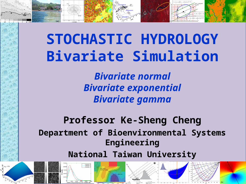
STOCHASTIC HYDROLOGYBivariate Simulation

Professor Ke-Sheng ChengDepartment of Bioenvironmental Systems Engineering

National Taiwan University

Bivariate normalBivariate exponential

Bivariate gamma

• Unlike the univariate stochastic simulation, bivariate simulation not only needs to consider the marginal densities but also the covariation of the two random variables.

04/19/23 2Laboratory for Remote Sensing Hydrology and Spatial Modeling, Dept of Bioenvironmental Systems Engineering, National Taiwan Univ.

Bivariate normal simulation I. Using conditional density

• Joint density

where and and are respectively the mean vector and covariance matrix of X1 and X2.

1

2

1

21

2

1)(

XXeX

)( 21 XXX T


• Conditional density

where i and i (i = 1, 2) are respectively the mean and standard deviation of Xi, and is the correlation coefficient between X1 and X2.

2

22

111

222

22122

1

)()(

2

1exp

)1(2

1)|(

xx

xxXf


• The conditional distribution of X2 given X1=x1 is also a normal distribution with mean and standard deviation respectively equal to and .

• Random number generation of a BVN distribution can be done by – Generating a random sample of X1, say

.

– Generating corresponding random sample of X2| x1, i.e. , using the conditional density.

111

22

x 2

2 1

),,,( 11211 nxxx

),,,( 22221 nxxx


Bivariate normal simulation II. Using the PC Transformation


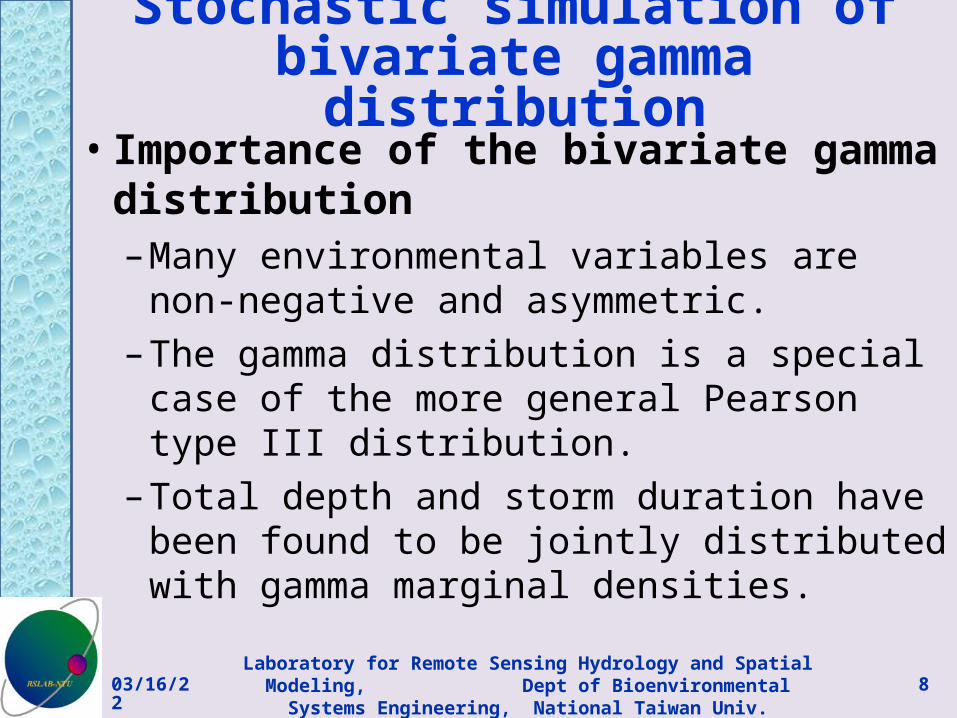
Stochastic simulation of bivariate gamma distribution

• Importance of the bivariate gamma distribution–Many environmental variables are non-

negative and asymmetric.– The gamma distribution is a special case of the

more general Pearson type III distribution.– Total depth and storm duration have been

found to be jointly distributed with gamma marginal densities.


• Many bivariate gamma distribution models are difficult to be implemented to solve practical problems, and seldom succeeded in gaining popularity among practitioners in the field of hydrological frequency analysis (Yue et al., 2001).

• Additionally, there is no agreement about what the multivariate gamma distribution should be and in practical applications we often only need to specify the marginal gamma distributions and the correlations between the component random variables (Law, 2007).


• Simulation of bivariate gamma distribution based on the frequency factor which is well-known to scientists and engineers in water resources field. – The proposed approach aims to yield random

vectors which have not only the desired marginal distributions but also a pre-specified correlation coefficient between component variates.


Rationale of BVG simulation using frequency factor

• From the view point of random number generation, the frequency factor can be considered as a random variable K, and KT is a value of K with exceedence probability 1/T.

• Frequency factor of the Pearson type III distribution can be approximated by

543

2

232

63

1

661

66

3

1

61

XXX

XXT

zz

zzzzK

[A]

Standard normal deviate


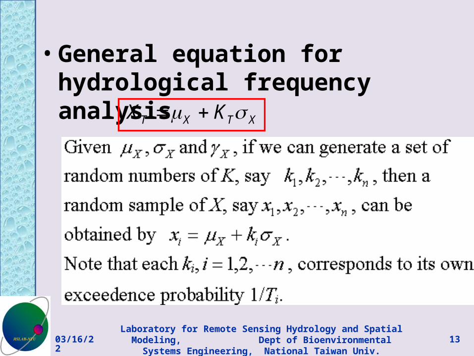
• General equation for hydrological frequency analysis

XTXT KX


• The gamma distribution is a special case of the Pearson type III distribution with a zero location parameter. Therefore, it seems plausible to generate random samples of a bivariate gamma distribution based on two jointly distributed frequency factors.

543

2

232

63

1

661

66

3

1

61

XXX

XXT

zz

zzzzK

[A]


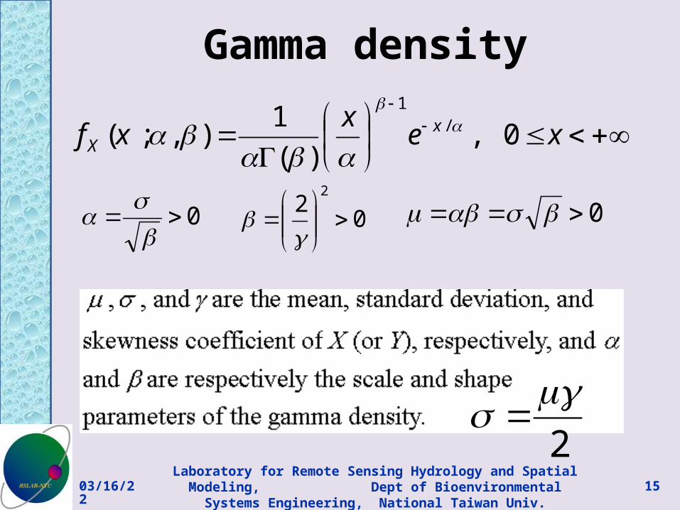
Gamma density

xex

xf xX 0,

)(

1),;( /

1

0

02

2

0

2


543

22

32

63

1

661

66

3

1

61

XXXXX

T zzzzzzK

• Assume two gamma random variables X and Y are jointly distributed.

• The two random variables are respectively associated with their frequency factors KX and KY .

• Equation (A) indicates that the frequency factor KX of a random variable X with gamma density is approximated by a function of the standard normal deviate and the coefficient of skewness of the gamma density.


543

22

32

63

1

661

66

3

1

61

XXXXX

T zzzzzzK


• Thus, random number generation of the second frequency factor KY must take into consideration the correlation between KX and KY which stems from the correlation between U and V.


Conditional normal density

• Given a random number of U, say u, the conditional density of V is expressed by the following conditional normal density

with mean and variance .

)|(| uUvUV

2

22 12

1exp

)1(2

1

UV

UV

UV

uv

uUV 21 UV


)|(| uUvUV

2

22 12

1exp

)1(2

1

UV

UV

UV

uv


XX KX


Flowchart of BVG simulation (1/2)


Flowchart of BVG simulation (2/2)


Conversion ~ UVXY

32 62

933

UVYXUVYX

UVYXYXYXYXXY

CCBB

CCACCAAA

4

61

X

XA 3

66

XX

XB 2

63

1

X

XC

4

61

Y

YA 3

66

YY

YB 2

63

1

Y

YC

[B]


• Frequency factors KX and KY can be respectively approximated by

where U and V both are random variables with standard normal density and are correlated with correlation coefficient .

543

22

32

63

1

661

66

3

1

61

XXXXX

X UUUUUUK

543

22

32

63

1

661

66

3

1

61

YYYYY

Y VVVVVVK

UV


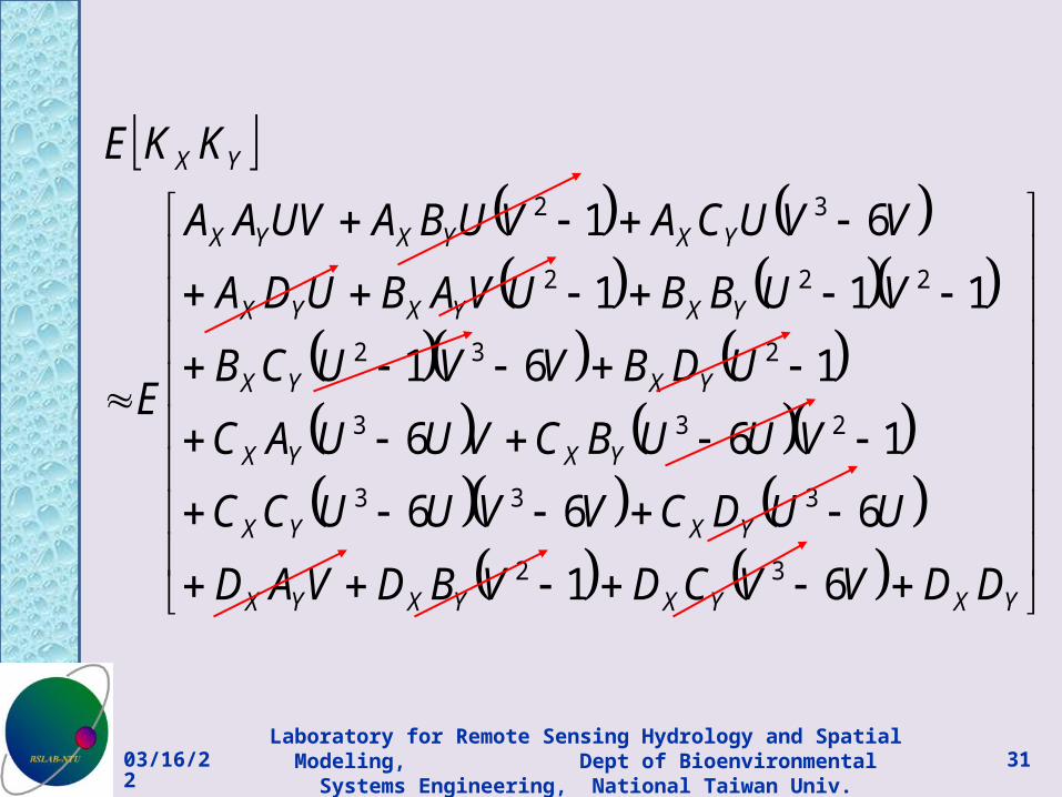
• Correlation coefficient of KX and KY can be derived as follows:

YXYXKK KKEKKCovYX

),(

543

22

32

5432

232

63

1

661

66

3

1

61

63

1

661

66

3

1

61

YYYYY

XXXXX

VVVVVV

UUUUUU

E


52

33

24

63

1

66

3

1

661

61

XXXXX

X UUUUK

XXXX DUUCUBUA 61 32

52

33

24

63

1

66

3

1

661

61

YYYYY

Y VVVVK

YYYY DVVCVBVA 61 32

5234

63

1,

63

1,

66,

61

X

XX

XXX

XX

X DCBA

5234

63

1,

63

1,

66,

61

Y

YY

YYY

YY

Y DCBA


YXYXYXYX

YXYX

YXYX

YXYX

YXYXYX

YXYXYX

YX

DDVVCDVBDVAD

UUDCVVUUCC

VUUBCVUUAC

UDBVVUCB

VUBBUVABUDA

VVUCAVUBAUVAA

E

KKE

61

666

166

161

111

61

32

333

233

232

222

32


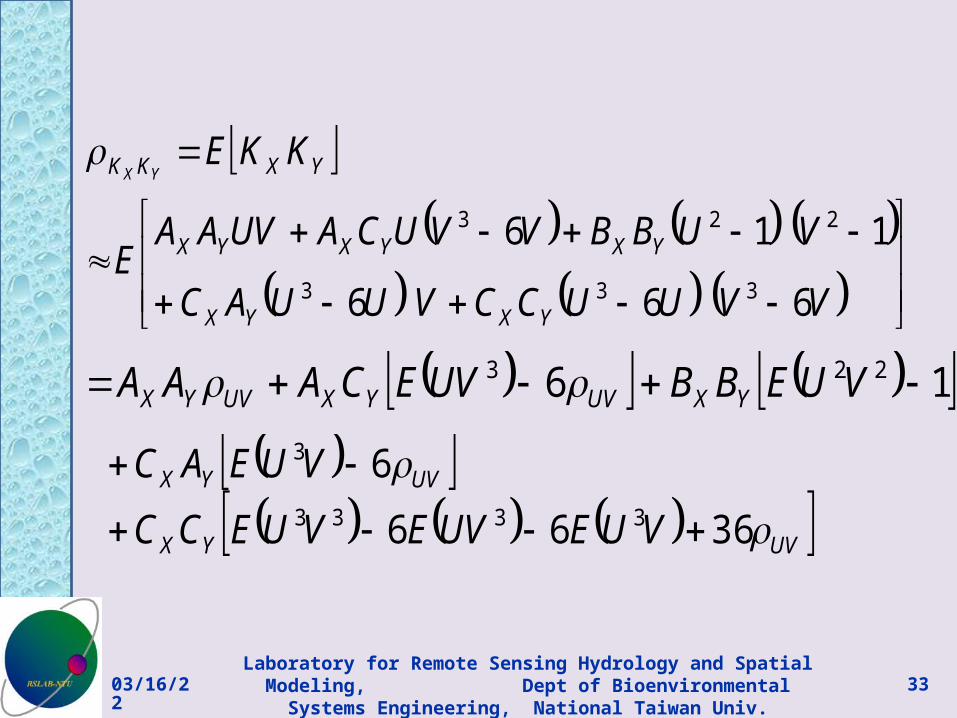
Since KX and KY are distributed with zero means, it follows that

YXKKE

YXYXYX

YXYXYX

DDVVUUCCVUUAC

VUBBVVUCAUVAAE

666

116333

223

XXXXXX DDUUCUBUAEKE 61][ 32

0 YX DD


VVUUCCVUUAC

VUBBVVUCAUVAAE

KKE

YXYX

YXYXYX

YXKK YX

666

116

333

223

16 223 VUEBBUVECAAA YXUVYXUVYX

UVYX

UVYX

VUEUVEVUECC

VUEAC

3666

63333

3


• It can also be shown that

Thus,

12 222 UVVUE UVUVVUE 96 333

UVUVEVUE 333

32 62

933

UVYXUVYX

UVYXYXYXYXKKXY

CCBB

CCACCAAAYX


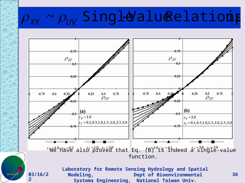
ipRelationsh Value-Single ~ UVXY

We have also proved that Eq. (B) is indeed a single-value function.


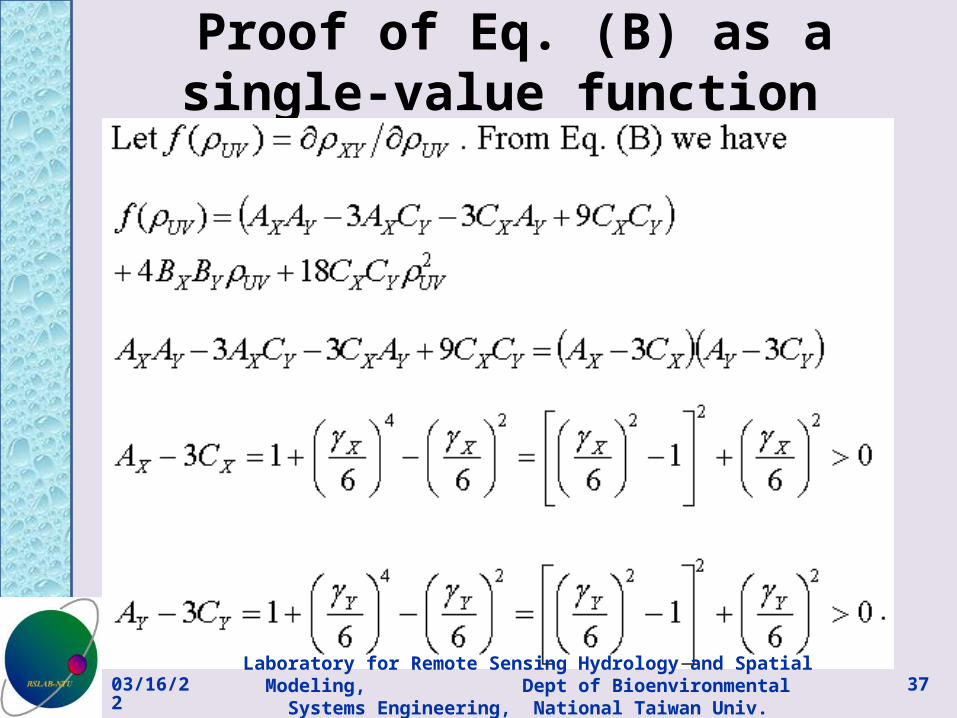
Proof of Eq. (B) as a single-value function


• Therefore,

YXYXYXYX CCACCAAA 933

222222

61

661

6YYXX


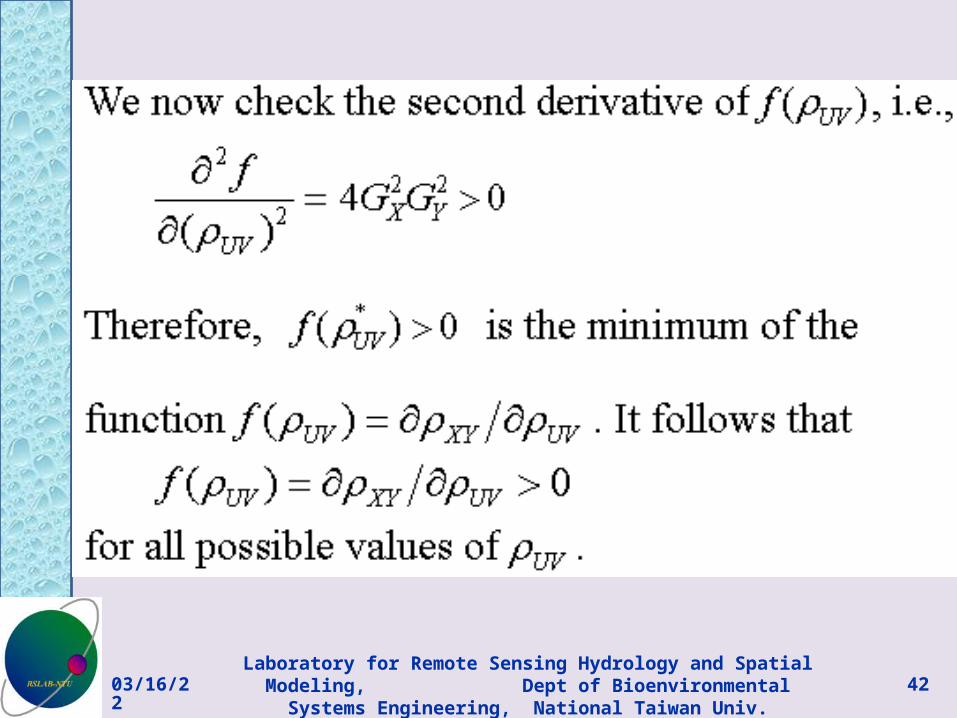
• The above equation indicates increases with increasing , and thus Eq. (B) is a single-value function.

XYUV


Simulation and validation • We chose to base our simulation on real

rainfall data observed at two raingauge stations (C1I020 and C1G690) in central Taiwan.

• Results of a previous study show that total rainfall depth (in mm) and duration (in hours) of typhoon events can be modeled as a joint gamma distribution.


Statistical properties of typhoon events at two raingauge stations


Assessing simulation results

• Variation of the sample means with respect to sample size n.

• Variation of the sample skewness with respect to sample size n.

• Variation of the sample correlation coefficient with respect to sample size n.

• Comparing CDF and ECDF• Scattering pattern of random samples


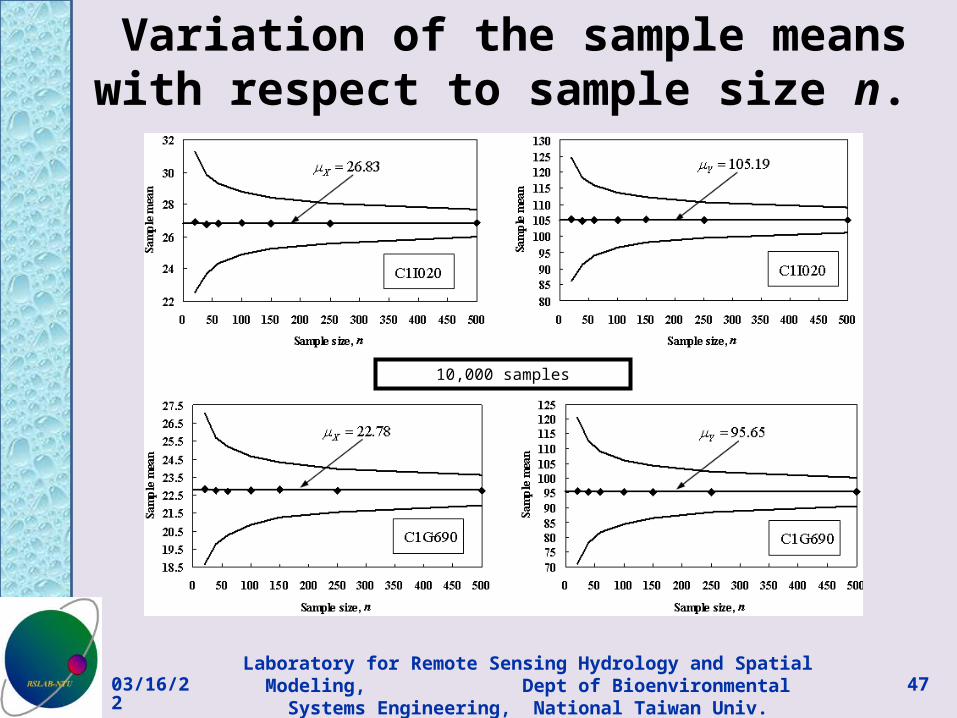
Variation of the sample means with respect to sample size n.

10,000 samples


Variation of the sample skewness with respect to sample size n.

10,000 samples


Variation of the sample correlation coefficient with respect to sample size n.

10,000 samples


Comparing CDF and ECDF


A scatter plot of simulated random samples with inappropriate pattern (adapted from Schmeiser and Lal,

1982).


Scattering of random samples


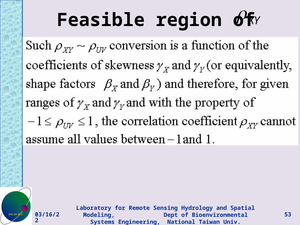
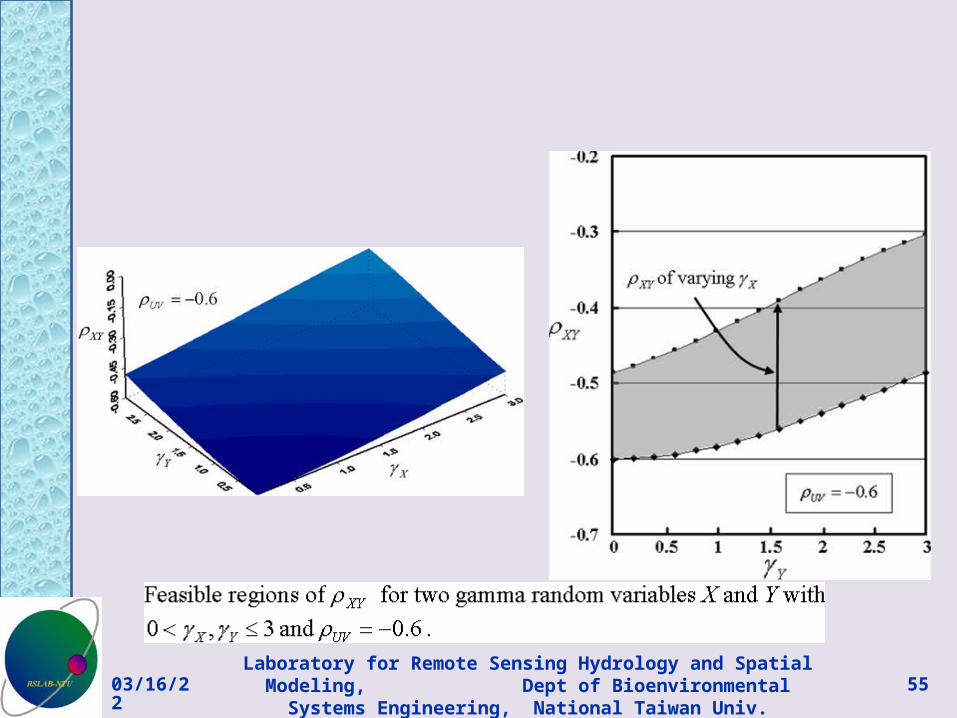
Feasible region of XY


Joint BVG Density • Random samples generated by the

proposed approach are distributed with the following joint PDF of the Moran bivariate gamma model:

)1(2

)(2)(exp

),;(),;(1

1),(

2

22

2

UV

UVUVUV

yyYxxX

UV

XY

vuvu

yfxfyxf

)],;([1xxX xFu )],;([1

yyY yFv


Stochastic Simulation of Bivariate Exponential Distribution

• A bivariate exponential distribution simulation algorithm was proposed by Marshall and Olkin (1967).

• Let X and Y be two jointly distributed exponenttial random variables. The joint exponential distribution function of Marshall and Olkin model (MOBED) has the following form:

Marshall, A.W. & Olkin, I. 1967. A Generalized Bivariate Exponential Distribution. Journal of Applied Probability, Vol. 4, 291-302.


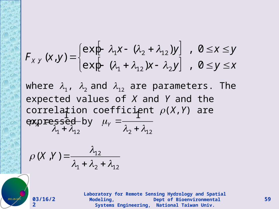
where 1, 2 and 12 are parameters. The expected values of X

and Y and the correlation coefficient (X,Y) are expressed by

0 , )(exp

0 , )(exp),(

2121

1221,

xyyx

yxyxyxF YX

121

1

X

122

1

Y

1221

12),(

YX


Simulation of the bivariate exponential distribution of Equation (1) is achieved by independently generating random numbers of three univariate exponential densities (Z1, Z2, and Z12) with

parameters 1, 2 and 12, respectively. Then a pair of

random number of (X,Y) is obtained by setting

x=min(z1, z12) and y=min(z2, z12).


61

Another example – target cancer risk

62

Modeling MCSinorg – Log-normal

63

Cumulative distribution of the target cancer risk

There is no need for stochastic simulation since the risk is completely dependent on only one random variable (MCS). Once the parameters of MCS are determined, the distribution of TR is completely specified.

STOCHASTIC HYDROLOGY Bivariate Simulation Professor Ke-Sheng Cheng Department of Bioenvironmental...

Documents

Transcript of STOCHASTIC HYDROLOGY Bivariate Simulation Professor Ke-Sheng Cheng Department of Bioenvironmental...