Stochastic Gravity: Theory and Applications - Springer · gravity theory is the vacuum ... quantum...

Living Rev. Relativity, 11, (2008), 3http://www.livingreviews.org/lrr-2008-3

(Update of lrr-2004-3)

http://relativity.livingreviews.org

L I V I N G REVIEWS

in relativity

Stochastic Gravity: Theory and Applications

Bei Lok HuDepartment of PhysicsUniversity of Maryland

College Park, Maryland 20742-4111U.S.A.

email: [email protected]://www.physics.umd.edu/people/faculty/hu.html

Enric VerdaguerDepartament de Fısica Fonamental and

Institut de Ciencies del CosmosUniversitat de Barcelona

Av. Diagonal 647, 08028 BarcelonaSpain

email: [email protected]

Living Reviews in RelativityISSN 1433-8351

Accepted on 11 April 2008Published on 29 May 2008

Abstract

Whereas semiclassical gravity is based on the semiclassical Einstein equation with sourcesgiven by the expectation value of the stress-energy tensor of quantum fields, stochastic semi-classical gravity is based on the Einstein–Langevin equation, which has, in addition, sourcesdue to the noise kernel. The noise kernel is the vacuum expectation value of the (operator-valued) stress-energy bitensor, which describes the fluctuations of quantum-matter fields incurved spacetimes. A new improved criterion for the validity of semiclassical gravity may alsobe formulated from the viewpoint of this theory. In the first part of this review we describethe fundamentals of this new theory via two approaches: the axiomatic and the functional.The axiomatic approach is useful to see the structure of the theory from the framework ofsemiclassical gravity, showing the link from the mean value of the stress-energy tensor to thecorrelation functions. The functional approach uses the Feynman–Vernon influence functionaland the Schwinger–Keldysh closed-time-path effective action methods. In the second part, wedescribe three applications of stochastic gravity. First, we consider metric perturbations in aMinkowski spacetime, compute the two-point correlation functions of these perturbations andprove that Minkowski spacetime is a stable solution of semiclassical gravity. Second, we discussstructure formation from the stochastic-gravity viewpoint, which can go beyond the standardtreatment by incorporating the full quantum effect of the inflaton fluctuations. Third, usingthe Einstein–Langevin equation, we discuss the backreaction of Hawking radiation and thebehavior of metric fluctuations for both the quasi-equilibrium condition of a black-hole in abox and the fully nonequilibrium condition of an evaporating black hole spacetime. Finally,we briefly discuss the theoretical structure of stochastic gravity in relation to quantum gravityand point out directions for further developments and applications.

This review is licensed under a Creative CommonsAttribution-Non-Commercial-NoDerivs 2.0 Germany License.http://creativecommons.org/licenses/by-nc-nd/2.0/de/

http://www.livingreviews.org/lrr-2008-3

http://www.physics.umd.edu/people/faculty/hu.html

http://creativecommons.org/licenses/by-nc-nd/2.0/de/

Imprint / Terms of Use

Living Reviews in Relativity is a peer reviewed open access journal published by the Max PlanckInstitute for Gravitational Physics, Am Muhlenberg 1, 14476 Potsdam, Germany. ISSN 1433-8351.

This review is licensed under a Creative Commons Attribution-Non-Commercial-NoDerivs 2.0Germany License: http://creativecommons.org/licenses/by-nc-nd/2.0/de/

Because a Living Reviews article can evolve over time, we recommend to cite the article as follows:

Bei Lok Hu and Enric Verdaguer,“Stochastic Gravity: Theory and Applications”,

Living Rev. Relativity, 11, (2008), 3. [Online Article]: cited [<date>],http://www.livingreviews.org/lrr-2008-3

The date given as <date> then uniquely identifies the version of the article you are referring to.

Article Revisions

Living Reviews supports two different ways to keep its articles up-to-date:

Fast-track revision A fast-track revision provides the author with the opportunity to add shortnotices of current research results, trends and developments, or important publications tothe article. A fast-track revision is refereed by the responsible subject editor. If an articlehas undergone a fast-track revision, a summary of changes will be listed here.

Major update A major update will include substantial changes and additions and is subject tofull external refereeing. It is published with a new publication number.

For detailed documentation of an article’s evolution, please refer always to the history documentof the article’s online version at http://www.livingreviews.org/lrr-2008-3.

http://creativecommons.org/licenses/by-nc-nd/2.0/de/


Contents

1 Overview 5

2 From Semiclassical to Stochastic Gravity 82.1 The importance of quantum fluctuations . . . . . . . . . . . . . . . . . . . . . . . . 8

3 The Einstein–Langevin Equation: Axiomatic Approach 113.1 Semiclassical gravity . . . . . . . . . . . . . . . . . . . . . . . . . . . . . . . . . . . 113.2 Stochastic gravity . . . . . . . . . . . . . . . . . . . . . . . . . . . . . . . . . . . . . 133.3 Validity of semiclassical gravity . . . . . . . . . . . . . . . . . . . . . . . . . . . . . 17

3.3.1 The large N expansion . . . . . . . . . . . . . . . . . . . . . . . . . . . . . . 18

4 The Einstein-Langevin Equation: Functional Approach 214.1 Influence action for semiclassical gravity . . . . . . . . . . . . . . . . . . . . . . . . 214.2 Influence action for stochastic gravity . . . . . . . . . . . . . . . . . . . . . . . . . 234.3 Explicit form of the Einstein-Langevin equation . . . . . . . . . . . . . . . . . . . . 25

4.3.1 The kernels for the vacuum state . . . . . . . . . . . . . . . . . . . . . . . . 26

5 Noise Kernel and Point Separation 285.1 Point separation . . . . . . . . . . . . . . . . . . . . . . . . . . . . . . . . . . . . . 29

5.1.1 n-tensors and end-point expansions . . . . . . . . . . . . . . . . . . . . . . . 295.2 Stress-energy bitensor operator and noise kernel . . . . . . . . . . . . . . . . . . . . 31

5.2.1 Finiteness of the noise kernel . . . . . . . . . . . . . . . . . . . . . . . . . . 325.2.2 Explicit form of the noise kernel . . . . . . . . . . . . . . . . . . . . . . . . 335.2.3 Trace of the noise kernel . . . . . . . . . . . . . . . . . . . . . . . . . . . . . 35

6 Metric Fluctuations in Minkowski Spacetime 376.1 Perturbations around Minkowski spacetime . . . . . . . . . . . . . . . . . . . . . . 376.2 The kernels in the Minkowski background . . . . . . . . . . . . . . . . . . . . . . . 396.3 The Einstein–Langevin equation . . . . . . . . . . . . . . . . . . . . . . . . . . . . 426.4 Correlation functions for gravitational perturbations . . . . . . . . . . . . . . . . . 44

6.4.1 Correlation functions for the linearized Einstein tensor . . . . . . . . . . . . 456.4.2 Correlation functions for the metric perturbations . . . . . . . . . . . . . . 476.4.3 Conformally-coupled field . . . . . . . . . . . . . . . . . . . . . . . . . . . . 48

6.5 Stability of Minkowski spacetime . . . . . . . . . . . . . . . . . . . . . . . . . . . . 496.5.1 Intrinsic metric fluctuations . . . . . . . . . . . . . . . . . . . . . . . . . . . 506.5.2 Induced metric fluctuations . . . . . . . . . . . . . . . . . . . . . . . . . . . 526.5.3 Order-reduction prescription and large N . . . . . . . . . . . . . . . . . . . 546.5.4 Summary . . . . . . . . . . . . . . . . . . . . . . . . . . . . . . . . . . . . . 55

7 Structure Formation in the Early Universe 577.1 The model . . . . . . . . . . . . . . . . . . . . . . . . . . . . . . . . . . . . . . . . . 577.2 Einstein–Langevin equation for scalar metric perturbations . . . . . . . . . . . . . 587.3 Correlation functions for scalar metric perturbations . . . . . . . . . . . . . . . . . 597.4 Summary and outlook . . . . . . . . . . . . . . . . . . . . . . . . . . . . . . . . . . 61

8 Black Hole Backreaction and Fluctuations 638.1 General issues of backreaction . . . . . . . . . . . . . . . . . . . . . . . . . . . . . . 63

8.1.1 Regularized energy-momentum tensor . . . . . . . . . . . . . . . . . . . . . 638.1.2 Backreaction and fluctuation-dissipation relation . . . . . . . . . . . . . . . 648.1.3 Noise and fluctuations – the missing ingredient in older treatments . . . . . 65

8.2 Backreaction on black holes under quasi-static conditions . . . . . . . . . . . . . . 658.2.1 The model . . . . . . . . . . . . . . . . . . . . . . . . . . . . . . . . . . . . 668.2.2 CTP effective action for the black hole . . . . . . . . . . . . . . . . . . . . . 678.2.3 Near flat case . . . . . . . . . . . . . . . . . . . . . . . . . . . . . . . . . . . 698.2.4 Near-horizon case . . . . . . . . . . . . . . . . . . . . . . . . . . . . . . . . . 718.2.5 Einstein–Langevin equation . . . . . . . . . . . . . . . . . . . . . . . . . . . 728.2.6 Comments . . . . . . . . . . . . . . . . . . . . . . . . . . . . . . . . . . . . . 74

8.3 Metric fluctuations of an evaporating black hole . . . . . . . . . . . . . . . . . . . . 758.3.1 Evolution of the mean geometry of an evaporating black hole . . . . . . . . 758.3.2 Spherically-symmetric induced fluctuations . . . . . . . . . . . . . . . . . . 778.3.3 Summary and prospects . . . . . . . . . . . . . . . . . . . . . . . . . . . . . 81

8.4 Other work on metric fluctuations but without backreaction . . . . . . . . . . . . . 82

9 Concluding Remarks 83

10 Acknowledgements 84

References 85

Stochastic Gravity: Theory and Applications 5

1 Overview

Stochastic semiclassical gravity is a theory developed in the 1990s using semiclassical gravity(quantum fields in classical spacetimes, the dynamics of both matter and spacetime are solvedself-consistently) as the starting point and aiming at a theory of quantum gravity as the goal.While semiclassical gravity is based on the semiclassical Einstein equation with the source givenby the expectation value of the stress-energy tensor of quantum fields, stochastic semiclassicalgravity, or stochastic gravity for short, also includes its fluctuations in a new stochastic semiclas-sical Einstein–Langevin equation (we will often use the shortened term stochastic gravity as thereis no confusion as to the nature and source of stochasticity in gravity being induced from thequantum fields and not a priori from the classical spacetime). If the centerpiece in semiclassical-gravity theory is the vacuum expectation value of the stress-energy tensor of a quantum field andthe central issues are how well the vacuum is defined and how the divergences can be controlledby regularization and renormalization, the centerpiece in stochastic semiclassical-gravity theory isthe stress-energy bitensor and its expectation value known as the noise kernel. The mathematicalproperties of this quantity and its physical content in relation to the behavior of fluctuations ofquantum fields in curved spacetimes are the central issues of this new theory. How they inducemetric fluctuations and seed the structures of the universe, how they affect the black-hole hori-zons and the backreaction of Hawking radiance in black hole dynamics, including implications fortrans-Planckian physics, are new horizons to explore. On theoretical issues, stochastic gravity isthe necessary foundation to investigate the validity of semiclassical gravity and the viability ofinflationary cosmology based on the appearance and sustenance of a vacuum energy-dominatedphase. It is also a useful beachhead supported by well-established low-energy (sub-Planckian)physics from which to explore the connection with high-energy (Planckian) physics in the realm ofquantum gravity.

In this review we summarize the major work and results of this theory since 1998. It is inthe nature of a progress report rather than a review. In fact we will have room only to discussa handful of topics of basic importance. A review of ideas leading to stochastic gravity and fur-ther developments originating from it can be found in [181, 187], a set of lectures, which includea discussion of the issue of the validity of semiclassical gravity in [207] and a pedagogical intro-duction of stochastic-gravity theory with a more detailed treatment of backreaction problems incosmology and black holes in quasi-equilibrium in [208]. A comprehensive formal description ofthe fundamentals is given in [257, 258], while that of the noise kernel in arbitrary spacetimes canbe found in [258, 304, 305]. Here we will try to mention related work so the reader can at leasttrace out the parallel and sequential developments. The references at the end of each topic beloware representative work in which one can seek out further treatments.

Stochastic gravity theory is built on three pillars: general relativity, quantum fields and nonequi-librium statistical mechanics. The first two uphold semiclassical gravity, the last two span statisticalfield theory. Strictly speaking one can understand a great deal without appealing to statistical me-chanics, and we will try to do so here. But concepts such as quantum open systems [88, 246, 370]and techniques such as the influence functional [107, 108] (which is related to the closed-time-patheffective action [14, 54, 56, 82, 87, 94, 222, 223, 227, 296, 323, 343]) were a great help in ourunderstanding of the physical meaning of issues involved in the construction of this new theory.Foremost because quantum fluctuations and correlation have ascended the stage and become thefocus of attention. Quantum statistical field theory and the statistical mechanics of quantum fieldtheory [55, 57, 59, 61] also aided us in searching for the connection with quantum gravity throughthe retrieval of correlations and coherence.

We show the scope of stochastic gravity as follows:

Living Reviews in Relativityhttp://www.livingreviews.org/lrr-2008-3


6 Bei Lok Hu and Enric Verdaguer

1 Ingredients:

(a) From General Relativity [266, 361] to Semiclassical Gravity.

(b) Quantum Field Theory in Curved Spacetimes [34, 121, 135, 362]:

i. Stress-energy tensor: Regularization and renormalization.ii. Self-consistent solution: Backreaction problems in early universe and black holes [3,

4, 5, 109, 137, 147, 148, 153, 154, 165, 193, 194, 251], and analog gravity [15, 16,252, 320, 321].

iii. Effective action: Closed time path, initial value formulation [14, 54, 56, 82, 87, 94,223, 227, 296, 323, 343].

iv. Equation of motion: Real and causal [222].

(c) Nonequilibrium Statistical Mechanics (see [62] and references therein) :

i. Open quantum systems [88, 246, 370].ii. Influence Functional: Stochastic equations [107, 108].iii. Noise and Decoherence: Quantum to classical transition [43, 46, 99, 100, 101, 126,

131, 136, 144, 145, 146, 149, 209, 210, 211, 212, 221, 228, 229, 230, 275, 276, 277,278, 279, 280, 299, 350, 352, 389, 390, 391, 392, 393].

(d) Decoherence in Quantum Cosmology and Emergence of Classical Spacetimes [50, 51,143, 182, 195, 231, 283].

2 Theory:

(a) Dissipation from Particle Creation [54, 72, 94, 222, 223, 296];Backreaction as Fluctuation-Dissipation Relation (FDR) [69, 76, 206, 268].

(b) Noise from Fluctuations of Quantum Fields [58, 181, 183].

(c) Einstein–Langevin Equations [52, 58, 73, 74, 192, 206, 248, 256, 257, 258].

(d) Metric Fluctuations in Minkowski spacetime [259].

3 Issues:

(a) Validity of Semiclassical Gravity [10, 111, 169, 170, 198, 203, 204, 223, 237, 303, 329].

(b) Viability of Vacuum Dominance and Inflationary Cosmology.

(c) Stress-Energy Bitensor and Noise Kernel: Regularization Reassessed [304, 305].

4 Applications: Early Universe and Black Holes:

(a) Wave Propagation in Stochastic Geometry [205].

(b) Black Hole Horizon Fluctuations: Spontaneous/Active versus Induced/Passive [20, 21,114, 261, 289, 305, 336, 338, 377].

(c) Noise induced inflation [67].

(d) Structure Formation [53, 60, 262, 263, 316];trace anomaly-driven inflation [162, 339, 355].

(e) Black Hole Backreaction and Fluctuations [69, 70, 76, 199, 200, 201, 268, 324, 325, 332].

5 Related Topics:

(a) Metric Fluctuations and Trans-Planckian Problem [20, 21, 261, 273, 289].

(b) Spacetime Foam, Loop and Spin Foam [32, 78, 79, 85, 116, 122, 123, 124, 271, 272].




(c) Universal ‘Metric Conductance’ Fluctuations [328].

6 Ideas:

(a) General Relativity as Geometro-Hydrodynamics [105, 164, 185, 189, 216, 356, 357];Emergent Gravity [139, 173, 240, 326].

(b) Semiclassical Gravity as Mesoscopic Physics [186, 190].

(c) From Stochastic to Quantum Gravity:

i. Via Correlation hierarchy of interacting quantum fields [57, 61, 187, 188].ii. Possible relation to string theory and matrix theory.iii. Other major approaches to quantum gravity [281].

For lack of space we list only the latest work in the respective topics above, describing ongoingresearch. The reader should consult the references therein for earlier work and background material.We do not seek a complete coverage here, but will discuss only those selected topics in theory, issuesand applications. We use the (+,+,+) sign conventions of [266, 361], and units in which c = ~ = 1.




2 From Semiclassical to Stochastic Gravity

There are three main steps that led to the recent development of stochastic gravity. The first stepbegins with quantum field theory in curved spacetime [34, 93, 121, 135, 362], which describes thebehavior of quantum matter fields propagating in a specified (not dynamically determined by thequantum matter field as source) background gravitational field. In this theory the gravitationalfield is given by the classical spacetime metric determined from classical sources by the classicalEinstein equations and the quantum fields propagate as test fields in such a spacetime. Someimportant processes described by quantum field theory in curved spacetime are particle creationfrom the vacuum, effects of vacuum fluctuations and polarizations in the early universe [29, 30, 31,81, 93, 117, 179, 293, 327, 386, 387], and Hawking radiation in black holes [155, 156, 213, 294, 358].

The second step in the description of the interaction of gravity with quantum fields is backre-action, i.e., the effect of quantum fields on spacetime geometry. The source here is the expectationvalue of the stress-energy operator for matter fields in some quantum state in the spacetime, aclassical observable. However, since this object is quadratic in the field operators, which are onlywell-defined as distributions on the spacetime, it involves ill-defined quantities. It contains ultra-violet divergences, the removal of which requires a renormalization procedure [83, 84, 93]. Thefinal expectation value of the stress-energy operator using a reasonable regularization technique isessentially unique, modulo some terms, which depend on the spacetime curvature and which areindependent of the quantum state. This uniqueness was proved by Wald [359, 360] who investi-gated the criteria that a physically meaningful expectation value of the stress-energy tensor oughtto satisfy.

The theory obtained from a self-consistent solution of the geometry of the spacetime and thequantum field is known as semiclassical gravity. Incorporating the backreaction of the quantummatter field into the spacetime is thus the central task in semiclassical gravity. One assumesa general class of spacetime, in which the quantum fields live and on which they act and seek asolution that satisfies simultaneously the Einstein equation for the spacetime and the field equationsfor the quantum fields. The Einstein equation, which has the expectation value of the stress-energyoperator of the quantum matter field as its source, is known as the semiclassical Einstein equation.Semiclassical gravity was first investigated in cosmological backreaction problems [3, 4, 109, 137,147, 148, 153, 154, 193, 194, 251]; an example is the damping of anisotropy in Bianchi universesby the backreaction of vacuum particle creation. The effect of quantum field processes, such asparticle creation, was used to explain why the universe is so isotropic at the present in the contextof chaotic cosmology [27, 28, 265] in the late 1970s prior to the inflationary-cosmology proposal ofthe 1980s [2, 140, 243, 244], which assumes the vacuum expectation value of an inflaton field asthe source, another, perhaps more well-known, example of semiclassical gravity.

2.1 The importance of quantum fluctuations

For a free quantum field, semiclassical gravity is fairly well understood. The theory is in somesense unique, since the only reasonable c-number stress-energy tensor that one may construct [359,360] with the stress-energy operator is a renormalized expectation value. However, the scopeand limitations of the theory are not so well understood. It is expected that the semiclassicaltheory will break down at the Planck scale. One can conceivably assume that it will also breakdown when the fluctuations of the stress-energy operator are large [111, 237]. Calculations of thefluctuations of the energy density for Minkowski, Casimir and hot flat spaces as well as Einsteinand de Sitter universes are available [86, 198, 237, 258, 259, 282, 302, 303, 304, 305, 313, 316].It is less clear, however, how to quantify what a large fluctuation is, and different criteria havebeen proposed [10, 11, 113, 115, 198, 237, 303, 384, 385]. The issue of the validity of semiclassicalgravity viewed in the light of quantum fluctuations was discussed in our Erice lectures [207]. More




recently in [203, 204] a new criterion has been proposed for the validity of semiclassical gravity.It is based on quantum fluctuations of the semiclassical metric and incorporates, in a unified andself-consistent way, previous criteria that have been used [10, 111, 169, 237]. One can see theessence of the validity problem in the following example inspired by Ford [111].

Let us assume a quantum state formed by an isolated system, which consists of a superpositionwith equal amplitude of one configuration of mass M with the center of mass at X1 and anotherconfiguration of the same mass with the center of mass atX2. The semiclassical theory, as describedby the semiclassical Einstein equation, predicts that the center of mass of the gravitational field ofthe system is centered at (X1 +X2)/2. However, one would expect that if we send a succession oftest particles to probe the gravitational field of the above system, half of the time they would reactto a gravitational field of mass M centered at X1 and half of the time to the field centered at X2.The two predictions are clearly different; note that the fluctuation in the position of the center ofmasses is on the order of (X1 − X2)2. Although this example raises the issue of the importanceof fluctuations to the mean, a word of caution should be added to the effect that it should not betaken too literally. In fact, if the previous masses are macroscopic, the quantum system decoheresvery quickly [392, 393] and, instead of being described by a pure quantum state, it is describedby a density matrix, which diagonalizes in a certain pointer basis. For observables associated withsuch a pointer basis, the density matrix description is equivalent to that provided by a statisticalensemble. The results will differ, in any case, from the semiclassical prediction.

In other words, one would expect that a stochastic source that describes the quantum fluc-tuations should enter into the semiclassical equations. A significant step in this direction wasmade in [181] where it was proposed that one view the backreaction problem in the frameworkof an open quantum system: the quantum fields acting as the “environment” and the gravi-tational field as the “system”. Following this proposal a systematic study of the connectionbetween semiclassical gravity and open quantum systems resulted in the development of a newconceptual and technical framework in which (semiclassical) Einstein–Langevin equations were de-rived [52, 58, 73, 74, 192, 206, 248]. The key technical factor to most of these results was the useof the influence-functional method of Feynman and Vernon [108], when only the coarse-grainedeffect of the environment on the system is of interest. Note that the word semiclassical put inparentheses refers to the fact that the noise source in the Einstein–Langevin equation arises fromthe quantum field, while the background spacetime is classical; generally we will not carry thisword since there is no confusion that the source, which contributes to the stochastic features ofthis theory, comes from quantum fields.

In the language of the consistent-histories formulation of quantum mechanics [43, 99, 100, 101,126, 136, 144, 145, 146, 149, 209, 210, 211, 212, 228, 229, 230, 275, 276, 277, 278, 279, 280, 299, 350],for the existence of a semiclassical regime for the dynamics of the system, one has two require-ments. The first is decoherence, which guarantees that probabilities can be consistently assignedto histories describing the evolution of the system, and the second is that these probabilities shouldpeak near histories, which correspond to solutions of classical equations of motion. The effect ofthe environment is crucial, on the one hand, to provide decoherence and, on the other hand, toproduce both dissipation and noise in the system through backreaction, thus inducing a semiclas-sical stochastic dynamic in the system. As shown by different authors [46, 127, 131, 221, 352,389, 390, 391, 392, 393], indeed over a long history predating the current revival of decoherence,stochastic semiclassical equations are obtained in an open quantum system after a coarse-grainingof the environmental degrees of freedom and a further coarse-graining in the system variables. Itis expected, but has not yet been shown, that this mechanism could also work for decoherenceand classicalization of the metric field. Thus far, the analogy could only be made formally [256] orunder certain assumptions, such as adopting the Born–Oppenheimer approximation in quantumcosmology [297, 298].

An alternative axiomatic approach to the Einstein–Langevin equation, without invoking the




open-system paradigm, was later suggested based on the formulation of a self-consistent dynamicalequation for a perturbative extension of semiclassical gravity able to account for the lowest-orderstress-energy fluctuations of matter fields [257]. It was shown that the same equation could bederived, in this general case, from the influence functional of Feynman and Vernon [258]. The fieldequation is deduced via an effective action, which is computed assuming that the gravitational fieldis a c-number. The important new element in the derivation of the Einstein–Langevin equation, andof stochastic-gravity theory, is the physical observable that measures the stress-energy fluctuations,namely, the expectation value of the symmetrized bitensor constructed with the stress-energy tensoroperator: the noise kernel. It is interesting to note that the Einstein–Langevin equation can alsobe understood as a useful intermediary tool to compute symmetrized two-point correlations ofthe quantum metric perturbations on the semiclassical background, independent of a suitableclassicalization mechanism [317].




3 The Einstein–Langevin Equation: Axiomatic Approach

In this section we introduce stochastic semiclassical gravity, or stochastic gravity for short, in anaxiomatic way. It is introduced as an extension of semiclassical gravity motivated by the search forself-consistent equations, which describe the backreaction of the quantum stress-energy fluctuationson the gravitational field [257].

3.1 Semiclassical gravity

Semiclassical gravity describes the interaction of a classical gravitational field with quantum matterfields. This theory can be formally derived as the leading 1/N approximation of quantum gravityinteracting withN independent and identical free quantum fields [152, 175, 176, 348], which interactwith gravity only. By keeping the value of NG finite, where G is Newton’s gravitational constant,one arrives at a theory in which formally the gravitational field can be treated as a c-number field(i.e., quantized at tree level) and matter fields are fully quantized. The semiclassical theory maybe summarized as follows.

Let (M, gab) be a globally hyperbolic four-dimensional spacetime manifold M with metric gaband consider a real scalar quantum field φ of mass m propagating on that manifold; we assume ascalar field for simplicity. The classical action Sm for this matter field is given by the functional

Sm[g, φ] = −12

∫d4x

√−g[gab∇aφ∇bφ+

(m2 + ξR

)φ2], (1)

where ∇a is the covariant derivative associated with the metric gab, ξ is a coupling parameterbetween the field and the scalar curvature of the underlying spacetime R and g = detgab.

The field may be quantized in the manifold using the standard canonical quantization formal-ism [34, 121, 362]. The field operator in the Heisenberg representation φ is an operator-valueddistribution solution of the Klein–Gordon equation,

(−m2 − ξR)φ = 0, (2)

where = ∇a∇a. We may write the field operator as φ[g;x) to indicate that it is a functional ofthe metric gab and a function of the spacetime point x. This notation will be used also for otheroperators and tensors.

The classical stress-energy tensor is obtained by functional derivation of this action in the usualway:

T ab(x) =2√−g

δSmδgab

, (3)

leading to

T ab[g, φ] = ∇aφ∇bφ− 12gab(∇cφ∇cφ+m2φ2

)+ξ(gab−∇a∇b +Gab

)φ2, (4)

where Gab is the Einstein tensor. With the notation T ab[g, φ] we explicitly indicate that thestress-energy tensor is a functional of the metric gab and the field φ.

The next step is to define a stress-energy tensor operator T ab[g;x). Naively, one would replacethe classical field φ[g;x) in the above functional with the quantum operator φ[g;x), but thisprocedure involves taking the product of two distributions at the same spacetime point; this is ill-defined and we need a regularization procedure. There are several regularization methods, whichone may use. One is the point-splitting or point-separation regularization method [83, 84], in whichone introduces a point y in the neighborhood of the point x and then uses as the regulator the




vector tangent at point x of the geodesic joining x and y; this method is discussed in [303, 304, 305]and in Section 5. Another well-known method is dimensional regularization, in which one works inn dimensions, where n is not necessarily an integer, and then uses as the regulator the parameterε = n − 4; this method is implicitly used in this section. The regularized stress-energy operatorusing the Weyl ordering prescription, i.e., symmetrical ordering, can be written as

T ab[g] =12∇aφ[g],∇bφ[g]+Dab[g] φ2[g], (5)

where Dab[g] is the differential operator

Dab ≡ (ξ − 1/4) gab + ξ(Rab −∇a∇b

). (6)

Note that if dimensional regularization is used, the field operator φ[g;x) propagates in an n-dimensional spacetime. Once the regularization prescription has been introduced, a regularizedand renormalized stress-energy operator TRab[g;x) may be defined as

TRab[g;x) = Tab[g;x) + FCab[g;x)I , (7)

which differs from the regularized Tab[g;x) by the identity operator times some tensor counter-terms FCab[g;x), which depend on the regulator and are local functionals of the metric; see [258]for details. The field states can be chosen in such a way that for any pair of physically acceptablestates, i.e., Hadamard states in the sense of [362], |ψ〉 and |ϕ〉, the matrix element 〈ψ|TRab|ϕ〉,defined as the limit when the regulator takes the physical value, is finite and satisfies Wald’saxioms [121, 359]. These counter-terms can be extracted from the singular part of a Schwinger–DeWitt series [44, 83, 84, 121]. The choice of these counter-terms is not unique, but this ambiguitycan be absorbed into the renormalized coupling constants, which appear in the equations of motionfor the gravitational field.

The semiclassical Einstein equation for the metric gab can then be written as

Gab[g] + Λgab − 2(αAab + βBab)[g] = 8πG〈TRab[g]〉, (8)

where 〈TRab[g]〉 is the expectation value of the operator TRab[g, x) after the regulator takes the phys-ical value in some physically acceptable state of the field on (M, gab). Note that both the stresstensor and the quantum state are functionals of the metric, hence the notation. The parametersG, Λ, α and β are the renormalized coupling constants, respectively the gravitational constant,the cosmological constant and two dimensionless coupling constants, which are zero in the classicalEinstein equation. These constants must be understood as the result of “dressing” the bare con-stants, which appear in the classical action before renormalization. The values of these constantsmust be determined by experiment. The left-hand side of Equation (8) may be derived from thegravitational action

Sg[g] =1

8πG

∫d4x

√−g[12R− Λ + αCabcdC

abcd + βR2

], (9)

where Cabcd is the Weyl tensor. The tensors Aab and Bab come from functional derivatives withrespect to the metric of the terms quadratic in the curvature in Equation (9); they are explicitly




given by

Aab =1√−g

δ

δgab

∫d4√−gCcdefCcdef

=12gabCcdefC

cdef − 2RacdeRbcde + 4RacR bc −

23RRab

−2Rab +23∇a∇bR+

13gabR, (10)

Bab =1√−g

δ

δgab

∫d4√−gR2

=12gabR2 − 2RRab + 2∇a∇bR− 2gabR, (11)

where Rabcd and Rab are the Riemann and Ricci tensors, respectively. These two tensors are, likethe Einstein and metric tensors, symmetric and divergence-less: ∇aAab = 0 = ∇aBab.

A solution of semiclassical gravity consists of a spacetime (M, gab), a quantum field operatorφ[g], which satisfies the evolution Equation (2) and a physically acceptable state |ψ[g]〉 for this field,such that Equation (8) is satisfied when the expectation value of the renormalized stress-energyoperator is evaluated in this state.

For a free quantum field this theory is robust in the sense that it is self-consistent and fairly wellunderstood. As long as the gravitational field is assumed to be described by a classical metric, theabove semiclassical Einstein equations seem to be the only plausible dynamical equation for thismetric: the metric couples to matter fields via the stress-energy tensor and for a given quantumstate the only physically observable c-number stress-energy tensor that one can construct is theabove renormalized expectation value. However, lacking a full quantum-gravity theory, the scopeand limits of the theory are not so well understood. It is assumed that the semiclassical theorywill break down at Planck scales, which is when simple order-of-magnitude estimates suggest thatthe quantum effects of gravity should not be ignored, because the energy of a quantum fluctuationin a Planck-size region, as determined by the Heisenberg uncertainty principle, is comparable tothe gravitational energy of that fluctuation.

The theory is expected to break down when the fluctuations of the stress-energy operator arelarge [111]. A criterion based on the ratio of the fluctuations to the mean was proposed by Kuoand Ford [237] (see also work over zeta-function methods [86, 302]). This proposal was questionedby Phillips and Hu [198, 303, 304] because it does not contain a scale at which the theory isprobed or how accurately the theory can be resolved. They suggested the use of a smearing scaleor point-separation distance for integrating over the bitensor quantities, which is equivalent toa stipulation of the resolution level of measurements; see also the response by Ford [113, 115].A different criterion was recently suggested by Anderson et al. [10, 11] based on linear-responsetheory. A partial summary of this issue can be found in our Erice Lectures [207].

More recently, in collaboration with A. Roura [203, 204], we have proposed a criterion for thevalidity of semiclassical gravity, which is based on the stability of the solutions of the semiclassicalEinstein equations with respect to quantum metric fluctuations. The two-point correlations forthe metric perturbations can be described in the framework of stochastic gravity, which is closelyrelated to the quantum theory of gravity interacting with N matter fields, to leading order in a1/N expansion. We will describe these developments in the following sections.

3.2 Stochastic gravity

The purpose of stochastic gravity is to extend semiclassical theory to account for these fluctuationsin a self-consistent way. A physical observable that describes these fluctuations to lowest order is




the noise kernel bitensor, which is defined through the two-point correlation of the stress-energyoperator as

Nabcd[g;x, y) =12〈tab[g;x), tcd[g; y)〉, (12)

where the curly brackets mean anticommutator, and where

tab[g;x) ≡ Tab[g;x)− 〈Tab[g;x)〉. (13)

This bitensor can also be writtenNab,c′d′ [g;x, y), orNab,c′d′(x, y) as we do in Section 5, to emphasizethat it is a tensor with respect to the first two indices at the point x and a tensor with respect tothe last two indices at the point y, but we shall not follow this notation here. The noise kernel isdefined in terms of the unrenormalized stress-tensor operator Tab[g;x) on a given background metricgab, thus a regulator is implicitly assumed on the right-hand side of Equation (12). However, for alinear quantum field, the above kernel – the expectation function of a bitensor – is free of ultravioletdivergences because the regularized Tab[g;x) differs from the renormalized TRab[g;x) by the identityoperator times some tensor counterterms (see Equation (7)) so that in the subtraction (13) thecounterterms cancel. Consequently the ultraviolet behavior of 〈Tab(x)Tcd(y)〉 is the same as thatof 〈Tab(x)〉〈Tcd(y)〉, and Tab can be replaced by the renormalized operator TRab in Equation (12);an alternative proof of this result is given in [304, 305]. The noise kernel should be thoughtof as a distribution function, the limit of coincidence points has meaning only in the sense ofdistributions. The bitensor Nabcd[g;x, y), or Nabcd(x, y) for short, is real and positive semi-definite,as a consequence of TRab being self-adjoint. A simple proof is given in [208].

Once the fluctuations of the stress-energy operator have been characterized, we can perturba-tively extend the semiclassical theory to account for such fluctuations. Thus we will assume thatthe background spacetime metric gab is a solution of the semiclassical Einstein equations (8) andwe will write the new metric for the extended theory as gab+hab, where we will assume that hab isa perturbation to the background solution. The renormalized stress-energy operator and the stateof the quantum field may now be denoted by TRab[g+h] and |ψ[g+h]〉, respectively, and 〈TRab[g+h]〉will be the corresponding expectation value.

Let us now introduce a Gaussian stochastic tensor field ξab[g;x) defined by the following cor-relators:

〈ξab[g;x)〉s = 0, 〈ξab[g;x)ξcd[g; y)〉s = Nabcd[g;x, y), (14)

where 〈. . . 〉s means statistical average. The symmetry and positive semi-definite property of thenoise kernel guarantees that the stochastic field tensor ξab[g, x), or ξab(x) for short, just introducedis well-defined. Note that this stochastic tensor captures only partially the quantum nature of thefluctuations of the stress-energy operator as it assumes that cumulants of higher order are zero.

An important property of this stochastic tensor is that it is covariantly conserved in the back-ground spacetime ∇aξab[g;x) = 0. In fact, as a consequence of the conservation of TRab[g] onecan see that ∇axNabcd(x, y) = 0. Taking the divergence in Equation (14) one can then showthat 〈∇aξab〉s = 0 and 〈∇axξab(x)ξcd(y)〉s = 0 so that ∇aξab is deterministic and represents withcertainty the zero vector field in M.

For a conformal field, i.e., a field whose classical action is conformally invariant, ξab is traceless:gabξab[g;x) = 0; so that, for a conformal matter field the stochastic source gives no correction to thetrace anomaly. In fact, from the trace anomaly result, which states that gabTRab[g] is, in this case, alocal c-number functional of gab times the identity operator, we have that gab(x)Nabcd[g;x, y) = 0.It then follows from Equation (14) that 〈gabξab〉s = 0 and 〈gab(x)ξab(x)ξcd(y)〉s = 0; an alternativeproof based on the point-separation method is given in [304, 305], see also Section 5.

All these properties make it quite natural to incorporate into the Einstein equations the stress-energy fluctuations by using the stochastic tensor ξab[g;x) as the source of the metric perturbations.




Thus we will write the following equation:

Gab[g+h]+Λ(gab+hab)− 2(αAab + βBab)[g+h]=8πG(〈TRab[g+h]〉+ξab[g]

). (15)

This equation is in the form of a (semiclassical) Einstein–Langevin equation; it is a dynamicalequation for the metric perturbation hab to linear order. It describes the backreaction of themetric to the quantum fluctuations of the stress-energy tensor of matter fields, and gives a first-order extension to semiclassical gravity as described by the semiclassical Einstein equation (8).

Note that we refer to the Einstein–Langevin equation as a first-order extension to the semi-classical Einstein equation of semiclassical gravity and the lowest-level representation of stochasticgravity. However, stochastic gravity has a much broader meaning; it refers to the range of theoriesbased on second and higher-order correlation functions. Noise can be defined in effectively-opensystems (e.g., correlation noise [61] in the Schwinger–Dyson equation hierarchy) to some degree,but one should not expect the Langevin form to prevail. In this sense we say stochastic gravityis the intermediate theory between semiclassical gravity (a mean field theory based on the expec-tation values of the energy momentum tensor of quantum fields) and quantum gravity (the fullhierarchy of correlation functions retaining complete quantum coherence [187, 188].

The renormalization of the operator Tab[g + h] is carried out exactly as in the previous case,now in the perturbed metric gab + hab. Note that the stochastic source ξab[g;x) is not dynamical;it is independent of hab, since it describes the fluctuations of the stress tensor on the semiclassicalbackground gab.

An important property of the Einstein–Langevin equation is that it is gauge invariant under thechange of hab by h′ab = hab +∇aζb +∇bζa, where ζa is a stochastic vector field on the backgroundmanifoldM. Note that a tensor such as Rab[g+h] transforms as Rab[g+h′] = Rab[g+h]+LζRab[g]to linear order in the perturbations, where Lζ is the Lie derivative with respect to ζa. Now, letus write the source tensors in Equations (15) and (8) to the left-hand sides of these equations. Ifwe substitute h with h′ in this new version of Equation (15), we get the same expression, with hinstead of h′, plus the Lie derivative of the combination of tensors, which appear on the left-handside of the new Equation (8). This last combination vanishes when Equation (8) is satisfied, i.e.,when the background metric gab is a solution of semiclassical gravity.

From the statistical average of Equation (15) we have that gab + 〈hab〉s must be a solution ofthe semiclassical Einstein equation linearized around the background gab; this solution has beenproposed as a test for the validity of the semiclassical approximation [10, 11] a point that will befurther discussed in Section 3.3.

The stochastic equation (15) predicts that the gravitational field has stochastic fluctuationsover the background gab. This equation is linear in hab, thus its solutions can be written as follows,

hab(x) = h0ab(x) + 8πG

∫d4x′

√−g(x′)Gret

abcd(x, x′)ξcd(x′), (16)

where h0ab(x) is the solution of the homogeneous equation containing information on the initial

conditions and Gretabcd(x, x

′) is the retarded propagator of Equation (15) with vanishing initialconditions. Form this we obtain the two-point correlation functions for the metric perturbations:

〈hab(x)hcd(y)〉s = 〈h0ab(x)h

0cd(y)〉s +

(8πG)2∫d4x′d4y′

√g(x′)g(y′)Gret

abef (x, x′)Nefgh(x′, y′)Gret

cdgh(y, y′)

≡ 〈hab(x)hcd(y)〉int + 〈hab(x)hcd(y)〉ind. (17)

There are two different contributions to the two-point correlations, which we have distinguishedin the second equality. The first one is connected to the fluctuations of the initial state of the




metric perturbations and we will refer to them as intrinsic fluctuations. The second contributionis proportional to the noise kernel and is thus connected with the fluctuations of the quantumfields; we will refer to them as induced fluctuations. To find these two-point stochastic correlationfunctions one needs to know the noise kernel Nabcd(x, y). Explicit expressions of this kernel interms of the two-point Wightman functions is given in [258], expressions based on point-splittingmethods have also been given in [304, 315]. Note that the noise kernel should be thought of as adistribution function, the limit of coincidence points has meaning only in the sense of distributions.

The two-point stochastic correlation functions for the metric perturbations of Equation (17)satisfy a very important property. In fact, it can be shown that they correspond exactly to thesymmetrized two-point correlation functions for the quantum metric perturbations in the large Nexpansion, i.e., the quantum theory describing the interaction of the gravitational field with Narbitrary free fields and expanded in powers of 1/N . To leading order for the graviton propagatorone finds that

〈hab(x), hcd(y)〉 = 2 〈hab(x)hcd(y)〉s, (18)

where hab(x) is the quantum operator corresponding to the metric perturbations and the statisticalaverage in Equation (17) for the homogeneous solutions is now taken with respect to the Wignerdistribution that describes the initial quantum state of the metric perturbations. The Lorentzgauge condition ∇a(hab − (1/2)ηabhcc) = 0, as well as an initial condition to completely fix thegauge of the initial state, should be implicitly understood. Moreover, since there are now Nscalar fields, the stochastic source has been rescaled so that the two-point correlation defined byEquation (14) should be 1/N times the noise kernel of a single field. This result was implicitlyobtained in the Minkowski background in [259] where the two-point correlation in the stochasticcontext was computed for the linearized metric perturbations. This stochastic correlation exactlyagrees with the symmetrized part of the graviton propagator computed by Tomboulis [348] in thequantum context of gravity interacting with N Fermion fields, where the graviton propagator is oforder 1/N . This result can be extended to an arbitrary background in the context of the large Nexpansion; a sketch of the proof with explicit details in the Minkowski background can be foundin [203]. This connection between the stochastic correlations and the quantum correlations wasnoted and studied in detail in the context of simpler open quantum systems [66]. Stochastic gravitygoes beyond semiclassical gravity in the following sense. The semiclassical theory, which is basedon the expectation value of the stress-energy tensor, carries information on the field two-pointcorrelations only, since 〈Tab〉 is quadratic in the field operator φ. The stochastic theory, on theother hand, is based on the noise kernel 12, which is quartic in the field operator. However, itdoes not carry information on the graviton-graviton interaction, which in the context of the largeN expansion gives diagrams of order 1/N2. This will be illustrated in Section 3.3.1. Furthermore,the retarded propagator also gives information on the commutator

〈[hab(x), hcd(y)]〉 = 16πiG(Gretabcd(y, x)−Gret

abcd(x, y)), (19)

so that combining the commutator with the anticommutator, the quantum two-point correlationfunctions are determined. Moreover, assuming a Gaussian initial state with vanishing expectationvalue for the metric perturbations, any n-point quantum correlation function is determined bythe two-point quantum correlations and thus by the stochastic approach. Consequently, one mayregard the Einstein–Langevin equation as a useful intermediary tool to compute the correlationfunctions for the quantum metric perturbations.

We should, however, also emphasize that Langevin-like equations are obtained to describethe quantum to classical transition in open quantum systems, when quantum decoherence takesplace by coarse-graining of the environment as well as by suitable coarse-graining of the systemvariables [101, 127, 144, 146, 150, 374]. In those cases the stochastic correlation functions describeactual classical correlations of the system variables. Examples can be found in the case of a




moving charged particle in an electromagnetic field in quantum electrodynamics [219] and in severalquantum Brownian models [64, 65, 66].

3.3 Validity of semiclassical gravity

As we have emphasized earlier, the scope and limits of semiclassical gravity are not well understoodbecause we still lack a fully well-understood quantum theory of gravity. From the semiclassicalEinstein equations it also seems clear that the semiclassical theory should break down when thequantum fluctuations of the stress tensor are large. Ford [111] was among the first to have empha-sized the importance of these quantum fluctuations. It is less clear, however, how to quantify thesize of these fluctuations. Kuo and Ford [237] used the variance of the fluctuations of the stresstensor operator compared to the mean value as a measure of the validity of semiclassical gravity.Hu and Phillips pointed out [198, 303] that such a criterion should be refined by considering thebackreaction of those fluctuations on the metric. Ford and collaborators also noticed that themetric fluctuations associated with the matter fluctuations can be meaningfully classified as ac-tive [114, 384, 385] and passive [111, 112, 115, 237], which correspond to our intrinsic and inducedfluctuations, respectively, and have studied their properties in different contexts [35, 36, 37]. How-ever, these fluctuations are not treated in a unified way and their precise relation to the quantumcorrelation function for the metric perturbations is not discussed. Furthermore, the full-averagedbackreaction of the matter fields is not included self-consistently and the contribution from thevacuum fluctuations in Minkowski space is discarded.

A different approach to the validity of semiclassical gravity was pioneered by Horowitz [169,170], who studied the stability of a semiclassical solution with respect to linear metric perturbations.In the case of a free quantum matter field in its Minkowski vacuum state, flat spacetime is asolution of semiclassical gravity. The equations describing those metric perturbations involvehigher-order derivatives and Horowitz found unstable runaway solutions that grow exponentiallywith characteristic timescales comparable to the Planck time; see also the analysis by Jordan [223].Later, Simon [329, 330] argued that those unstable solutions lie beyond the expected domain ofvalidity of the theory and emphasized that only those solutions, which resulted from truncatingperturbative expansions in terms of the square of the Planck length, are physically acceptable [329,330]. Further discussion was provided by Flanagan and Wald [110], who advocated the use of anorder-reduction prescription first introduced by Parker and Simon [295]. More recently Anderson,Molina-Parıs and Mottola have taken up the issue of the validity of semiclassical gravity [10,11] again. Their starting point is the fact that the semiclassical Einstein equation will fail toprovide a valid description of the dynamics of the mean spacetime geometry whenever the higher-order radiative corrections to the effective action, involving loops of gravitons or internal gravitonpropagators, become important. Next, they argue qualitatively that such higher-order radiativecorrections cannot be neglected if the metric fluctuations grow without bound. Finally, theypropose a criterion to characterize the growth of the metric fluctuations, and hence the validity ofsemiclassical gravity, based on the stability of the solutions of the linearized semiclassical equation.Following these approaches, the Minkowski metric is shown to be a stable solution of semiclassicalgravity with respect to small metric perturbations.

As emphasized in [10, 11] the above criteria may be understood as based on semiclassical gravityitself. It is certainly true that stability is a necessary condition for the validity of a semiclassicalsolution, but one may also look for criteria within extensions of semiclassical gravity. In the absenceof a quantum theory of gravity, such criteria may be found in some more modest extensions. Thus,Ford [111] considered graviton production in linearized quantum gravity and compared the resultswith the production of gravitational waves in semiclassical gravity. Ashtekar [13] and Beetle [22]found large quantum-gravity effects in three-dimensional quantum-gravity models. In a more recentpaper [203] (see also [204]), we advocate for a criteria within the stochastic gravity approach and




since stochastic gravity extends semiclassical gravity by incorporating the quantum stress-tensorfluctuations of the matter fields, this criteria is structurally the most complete to date.

It turns out that this validity criteria is equivalent to the validity criteria that one mightadvocate within the large N expansion; that is the quantum theory describing the interaction ofthe gravitational field with N identical free matter fields. In the leading order, namely the limitin which N goes to infinity and the gravitational constant is appropriately rescaled, the theoryreproduces semiclassical gravity. Thus, a natural extension of semiclassical gravity is providedby the next to leading order. It turns out that the symmetrized two-point quantum-correlationfunctions of the metric perturbations in the large N expansion are equivalent to the two-pointstochastic metric-correlation functions predicted by stochastic gravity. Our validity criterion canthen be formulated as follows: a solution of semiclassical gravity is valid when it is stable withrespect to quantum metric perturbations. This criterion involves the consideration of quantum-correlation functions of the metric perturbations, since the quantum field describing the metricperturbations hab(x) is characterized not only by its expectation value but also by its n-pointcorrelation functions.

It is important to emphasize that the above validity criterion incorporates in a unified and self-consistent way the two main ingredients of the criteria exposed above. Namely, the criteria based onthe quantum stress-tensor fluctuations of the matter fields, and the criteria based on the stability ofsemiclassical solutions against classical metric perturbations. The former is incorporated throughthe induced metric fluctuations, and the later through the intrinsic fluctuations introduced inEquation (17). Whereas information on the stability of intrinsic-metric fluctuations can be obtainedfrom an analysis of the solutions of the perturbed semiclassical Einstein equation (the homogeneouspart of Equation (15)), the effect of induced-metric fluctuations is accounted for only in stochasticgravity (the full inhomogeneous Equation (15)). We will illustrate these criteria in Section 6.5 bystudying the stability of Minkowski spacetime as a solution of semiclassical gravity.

3.3.1 The large N expansion

To illustrate the relation between the semiclassical, stochastic and quantum theories, a simplifiedmodel of scalar gravity interacting with N scalar fields is considered here.

The large N expansion has been successfully used in quantum chromodynamics to computesome nonperturbative results. This expansion re-sums and rearranges Feynman perturbative series,including self-energies. For gravity interacting with N matter fields, it shows that graviton loopsare of higher order than matter loops. To illustrate the large N expansion, let us first consider thefollowing toy model of gravity, which we will simplify as a scalar field h, interacting with a singlescalar field φ described by the action

S =1κ

∫d4x (∂ah∂ah+ h ∂ah∂

ah+ . . . )

−∫d4x

(∂aφ∂

aφ+m2φ2)

+∫d4x (h ∂aφ∂aφ+ . . . ) , (20)

where κ = 8πG and we have assumed that the interaction is linear in the (dimensionless) scalargravitational field h and quadratic in the matter field φ to simulate in a simplified way the couplingof the metric with the stress tensor of the matter fields. We have also included a self-coupling gravi-ton term of O(h3), which also appears in perturbative gravity beyond the linear approximation.

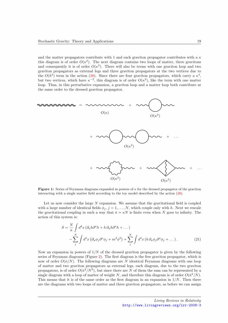
We may now compute the graviton dressed propagator perturbatively as the following series ofFeynman diagrams (Figure 1). The first diagram is just the free graviton propagator, which is ofO(κ), as one can see from the kinetic term for the graviton in Equation (20). The next diagramis one loop of matter with two external legs, which are the graviton propagators. This diagramhas two vertices with one graviton propagator and two matter field propagators. Since the vertices




and the matter propagators contribute with 1 and each graviton propagator contributes with a κthis diagram is of order O(κ2). The next diagram contains two loops of matter, three gravitonsand consequently it is of order O(κ3). There will also be terms with one graviton loop and twograviton propagators as external legs and three graviton propagators at the two vertices due tothe O(h3) term in the action (20). Since there are four graviton propagators, which carry a κ4,but two vertices, which have κ−2, this diagram is of order O(κ2), like the term with one matterloop. Thus, in this perturbative expansion, a graviton loop and a matter loop both contribute atthe same order to the dressed graviton propagator.

=

O(κ)

+

O(κ2)

+

O(κ3)

+ . . .

+

O(κ2)

+

O(κ3)

+ . . .

Figure 1: Series of Feynman diagrams expanded in powers of κ for the dressed propagator of the gravitoninteracting with a single matter field according to the toy model described by the action (20).

Let us now consider the large N expansion. We assume that the gravitational field is coupledwith a large number of identical fields φj , j = 1, . . . , N , which couple only with h. Next we rescalethe gravitational coupling in such a way that κ = κN is finite even when N goes to infinity. Theaction of this system is:

S =N

κ

∫d4x (∂ah∂ah+ h ∂ah∂

ah+ . . . )

−N∑j

∫d4x

(∂aφj∂

aφj +m2φ2)

+N∑j

∫d4x (h ∂aφj∂aφj + . . . ) . (21)

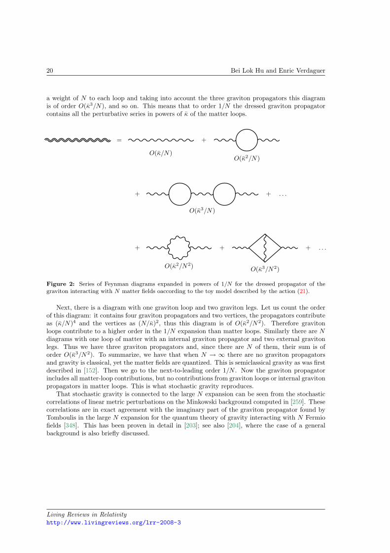
Now an expansion in powers of 1/N of the dressed graviton propagator is given by the followingseries of Feynman diagrams (Figure 2). The first diagram is the free graviton propagator, which isnow of order O(κ/N). The following diagrams are N identical Feynman diagrams with one loopof matter and two graviton propagators as external legs, each diagram, due to the two gravitonpropagators, is of order O(κ2/N2), but since there are N of them the sum can be represented by asingle diagram with a loop of matter of weight N , and therefore this diagram is of order O(κ2/N).This means that it is of the same order as the first diagram in an expansion in 1/N . Then thereare the diagrams with two loops of matter and three graviton propagators, as before we can assign




a weight of N to each loop and taking into account the three graviton propagators this diagramis of order O(κ3/N), and so on. This means that to order 1/N the dressed graviton propagatorcontains all the perturbative series in powers of κ of the matter loops.

=

O(κ/N)

+

O(κ2/N)

+

O(κ3/N)

+ . . .

+

O(κ2/N2)

+

O(κ3/N2)

+ . . .

Figure 2: Series of Feynman diagrams expanded in powers of 1/N for the dressed propagator of thegraviton interacting with N matter fields oaccording to the toy model described by the action (21).

Next, there is a diagram with one graviton loop and two graviton legs. Let us count the orderof this diagram: it contains four graviton propagators and two vertices, the propagators contributeas (κ/N)4 and the vertices as (N/κ)2, thus this diagram is of O(κ2/N2). Therefore gravitonloops contribute to a higher order in the 1/N expansion than matter loops. Similarly there are Ndiagrams with one loop of matter with an internal graviton propagator and two external gravitonlegs. Thus we have three graviton propagators and, since there are N of them, their sum is oforder O(κ3/N2). To summarize, we have that when N → ∞ there are no graviton propagatorsand gravity is classical, yet the matter fields are quantized. This is semiclassical gravity as was firstdescribed in [152]. Then we go to the next-to-leading order 1/N . Now the graviton propagatorincludes all matter-loop contributions, but no contributions from graviton loops or internal gravitonpropagators in matter loops. This is what stochastic gravity reproduces.

That stochastic gravity is connected to the large N expansion can be seen from the stochasticcorrelations of linear metric perturbations on the Minkowski background computed in [259]. Thesecorrelations are in exact agreement with the imaginary part of the graviton propagator found byTomboulis in the large N expansion for the quantum theory of gravity interacting with N Fermiofields [348]. This has been proven in detail in [203]; see also [204], where the case of a generalbackground is also briefly discussed.




4 The Einstein-Langevin Equation: Functional Approach

The Einstein–Langevin equation (15) may also be derived by a method based on functional tech-niques [258]. Here we will summarize these techniques starting with semiclassical gravity.

In semiclassical gravity functional methods were used to study the backreaction of quantumfields in cosmological models [109, 147, 153]. The primary advantage of the effective-action ap-proach is, in addition to the well-known fact that it is easy to introduce perturbation schemes likeloop expansion and nPI formalisms, that it yields a fully self-consistent solution. (For a generaldiscussion in the semiclassical context of these two approaches, equation of motion versus effectiveaction, contrast, e.g., [137, 193, 194, 251] with the above references and [3, 4, 148, 154]. Seealso comments in Section 8 on the black-hole backreaction problem comparing the approach byYork et al. [380, 381, 382] to that of Sinha, Raval and Hu [332].

The well known in-out effective-action method treated in textbooks, however, led to equations ofmotion, which were not real because they were tailored to compute transition elements of quantumoperators rather than expectation values. The correct technique to use for the backreaction problemis the Schwinger–Keldysh [14, 56, 82, 87, 227, 323, 343] closed-time-path (CTP) or ‘in-in’ effectiveaction. These techniques were adapted to the gravitational context [54, 72, 94, 222, 223, 296] andapplied to different problems in cosmology. One could deduce the semiclassical Einstein equationfrom the CTP effective action for the gravitational field (at tree level) with quantum matter fields.

Furthermore, in this case the CTP functional formalism turns out to be related [58, 69, 70,73, 134, 239, 247, 256, 258, 267, 343] to the influence-functional formalism of Feynman and Ver-non [108], since the full quantum system may be understood as consisting of a distinguished subsys-tem (the “system” of interest) interacting with the remaining degrees of freedom (the environment).Integrating out the environment variables in a CTP path integral yields the influence functional,from which one can define an effective action for the dynamics of the system [58, 134, 191, 206]. Thisapproach to semiclassical gravity is motivated by the observation [181] that in some open quantumsystems classicalization and decoherence [46, 131, 221, 352, 389, 390, 391, 392, 393] on the systemmay be brought about by interaction with an environment, the environment being in this case thematter fields and some “high-momentum” gravitational modes [50, 51, 143, 182, 195, 231, 283, 374].Unfortunately, since the form of a complete quantum theory of gravity interacting with matter isunknown, we do not know what these “high-momentum” gravitational modes are. Such a fun-damental quantum theory might not even be a field theory, in which case the metric and scalarfields would not be fundamental objects [187]. Thus, in this case, we cannot attempt to evaluatethe influence action of Feynman and Vernon starting from the fundamental quantum theory andperforming the path integrations in the environment variables. Instead, we introduce the influenceaction for an effective quantum field theory of gravity and matter [95, 96, 97, 98, 297, 298, 331], inwhich such “high-momentum” gravitational modes are assumed to have already been “integratedout.”

4.1 Influence action for semiclassical gravity

Let us formulate semiclassical gravity in this functional framework. Adopting the usual procedureof effective field theories [63, 95, 96, 97, 98, 366, 367], one has to take the effective action forthe metric and the scalar field of the most general local form compatible with general covariance:S[g, φ] ≡ Sg[g] + Sm[g, φ] + . . . , where Sg[g] and Sm[g, φ] are given by Equations (9) and (1),respectively, and the dots stand for terms of order higher than two in the curvature and in thenumber of derivatives of the scalar field. Here, we shall neglect the higher-order terms as well asself-interaction terms for the scalar field. The second order terms are necessary to renormalizeone-loop ultraviolet divergences of the scalar field stress-energy tensor, as we have already seen.Since M is a globally hyperbolic manifold, we can foliate it by a family of t = constant Cauchy




hypersurfaces Σt, and we will indicate the initial and final times by ti and tf , respectively.The influence functional corresponding to the action (1) describing a scalar field in a spacetime

(coupled to a metric field) may be introduced as a functional of two copies of the metric, denotedby g+

ab and g−ab, which coincide at some final time t = tf . Let us assume that, in the quantumeffective theory, the state of the full system (the scalar and the metric fields) in the Schrodingerpicture at the initial time t = ti can be described by a density operator, which can be written asthe tensor product of two operators on the Hilbert spaces of the metric and of the scalar field. Letρi(ti) ≡ ρi [φ+(ti), φ−(ti)] be the matrix element of the density operator ρS(ti) describing the initialstate of the scalar field. The Feynman–Vernon influence functional is defined as the following pathintegral over the two copies of the scalar field:

FIF[g±] ≡∫Dφ+Dφ− ρi(ti)δ [φ+(tf)− φ−(tf)] ei(Sm[g+,φ+]−Sm[g−,φ−]). (22)

Alternatively, the above double path integral can be rewritten as a CTP integral, namely, as asingle path integral in a complex time contour with two different time branches, one going forwardin time from ti to tf and the other going backward in time from tf to ti (in practice one usuallytakes ti → −∞). From this influence functional, the influence action SIF[g+, g−], or SIF[g±] forshort, defined by

FIF[g±] ≡ eiSIF[g±], (23)

carries all the information about the environment (the matter fields) relevant to the system (thegravitational field). Then we can define the CTP effective action for the gravitational field, Seff [g±],as

Seff [g±] ≡ Sg[g+]− Sg[g−] + SIF[g±]. (24)

This is the effective action for the classical gravitational field in the CTP formalism. However,since the gravitational field is treated only at the tree level, this is also the effective classical actionfrom which the classical equations of motion can be derived.

Expression (22) contains ultraviolet divergences and must be regularized. We shall assume thatdimensional regularization can be applied, that is, it makes sense to dimensionally continue all thequantities that appear in Equation (22). For this we need to work with the n-dimensional actionscorresponding to Sm in Equation (22) and Sg in Equation (9). For example, the parameters G,Λ, α, and β of Equation (9) are the bare parameters GB, ΛB, αB, and βB, and in Sg[g], insteadof the square of the Weyl tensor in Equation (9), one must use 2

3 (RabcdRabcd − RabRab), which

by the Gauss–Bonnet theorem leads to the same equations of motion as the action (9) whenn = 4. The form of Sg in n dimensions is suggested by the Schwinger–DeWitt analysis of theultraviolet divergences in the matter stress-energy tensor using dimensional regularization. Onecan then write the Feynman–Vernon effective action Seff [g±] in Equation (24) in a form suitable fordimensional regularization. Since both Sm and Sg contain second-order derivatives of the metric,one should also add some boundary terms [206, 361]. The effect of these terms is to cancel out theboundary terms, which appear when taking variations of Seff [g±], keeping the value of g+

ab and g−abfixed at Σti and Σtf . Alternatively, in order to obtain the equations of motion for the metric inthe semiclassical regime, we can work with the action terms without boundary terms and neglectall boundary terms when taking variations with respect to g±ab. From now on, all the functionalderivatives with respect to the metric will be understood in this sense.

The semiclassical Einstein equation (8) can now be derived. Using the definition of the stress-energy tensor T ab(x) = (2/

√−g)δSm/δgab and the definition of the influence functional, Equa-

tions (22) and (23), we see that

〈T ab[g;x)〉 =2√−g(x)

δSIF[g±]δg+ab(x)

∣∣∣∣∣g±=g

, (25)




where the expectation value is taken in the n-dimensional spacetime generalization of the statedescribed by ρS(ti). Therefore, differentiating Seff [g±] in Equation (24) with respect to g+

ab andthen setting g+

ab = g−ab = gab, we get the semiclassical Einstein equation in n dimensions. Thisequation is then renormalized by absorbing the divergences in the regularized 〈T ab[g]〉 into the bareparameters. Taking the limit n→ 4 we obtain the physical semiclassical Einstein equation (8).

4.2 Influence action for stochastic gravity

In the spirit of the previous derivation of the Einstein–Langevin equation, we now seek a dynamicalequation for a linear perturbation hab to the semiclassical metric gab, solution of Equation (8).Strictly speaking, if we use dimensional regularization we must consider the n-dimensional versionof that equation. From the results just described, if such an equation were simply a linearizedsemiclassical Einstein equation, it could be obtained from an expansion of the effective actionSeff [g + h±]. In particular, since, from Equation (25), we have that

〈T ab[g + h;x)〉 =2√

−det (g + h)(x)δSIF[g + h±]δh+

ab(x)

∣∣∣∣∣h±=h

, (26)

the expansion of 〈T ab[g + h]〉 to linear order in hab can be obtained from an expansion of theinfluence action SIF[g + h±] up to second order in h±ab.

To perform the expansion of the influence action, we have to compute the first and second orderfunctional derivatives of SIF[g + h±] and then set h+

ab = h−ab = hab. If we do so using the pathintegral representation (22), we can interpret these derivatives as expectation values of operators.The relevant second order derivatives are

4√−g(x)

√−g(y)

δ2SIF[g + h±]δh+ab(x)δh

+cd(y)

∣∣∣∣∣h±=h

= −HabcdS [g;x, y)−Kabcd[g;x, y) + iNabcd[g;x, y),

4√−g(x)

√−g(y)

δ2SIF[g±]δh+ab(x)δh

−cd(y)

∣∣∣∣∣h±=h

= −HabcdA [g;x, y)− iNabcd[g;x, y),

(27)

where

Nabcd[g;x, y) ≡ 12⟨tab[g;x), tcd[g; y)

⟩,

HabcdS [g;x, y) ≡ Im

⟨T∗(T ab[g;x)T cd[g; y)

)⟩,

HabcdA [g;x, y) ≡ − i

2

⟨[T ab[g;x), T cd[g; y)

]⟩,

Kabcd[g;x, y) ≡ −4√−g(x)

√−g(y)

⟨δ2Sm[g + h, φ]δhab(x)δhcd(y)

∣∣∣∣φ=φ

⟩,

with tab defined in Equation (13); [ , ] denotes the commutator and , the anti-commutator.Here we use a Weyl ordering prescription for the operators. The symbol T∗ denotes the followingordered operations: First, time order the field operators φ and then apply the derivative operators,which appear in each term of the product T ab(x)T cd(y), where T ab is the functional (4). ThisT∗ “time ordering” arises because we have path integrals containing products of derivatives ofthe field, which can be expressed as derivatives of the path integrals, which do not contain suchderivatives. Notice, from their definitions, that all the kernels, which appear in expressions (27),are real and also Habcd

A is free of ultraviolet divergences in the limit as n→ 4.




From Equations (25) and (25), since SIF[g, g] = 0 and SIF[g−, g+] = −S∗IF[g+, g−], we can writethe expansion for the influence action SIF[g+ h±] around a background metric gab in terms of theprevious kernels. Taking into account that these kernels satisfy the symmetry relations

HabcdS (x, y) = Hcdab

S (y, x), HabcdA (x, y) = −Hcdab

A (y, x), Kabcd(x, y) = Kcdab(y, x), (28)

and introducing the new kernel

Habcd(x, y) ≡ HabcdS (x, y) +Habcd

A (x, y), (29)

the expansion of SIF can be finally written as

SIF[g + h±] =12

∫d4x

√−g(x)〈T ab[g;x)〉 [hab(x)]

−18

∫d4x d4y

√−g(x)

√−g(y) [hab(x)]

(Habcd[g;x, y) +Kabcd[g;x, y)

)hcd(y)

+i

8

∫d4x d4y

√−g(x)

√−g(y) [hab(x)]Nabcd[g;x, y) [hcd(y)] +O(h3), (30)

where we have used the notation

[hab] ≡ h+ab − h−ab, hab ≡ h+

ab + h−ab. (31)

From Equations (26) and (30) it is clear that the imaginary part of the influence action does notcontribute to the perturbed semiclassical Einstein equation (the expectation value of the stress-energy tensor is real). However, as it depends on the noise kernel, it contains information on thefluctuations of the operator T ab[g].

We are now in a position to carry out the derivation of the semiclassical Einstein–Langevinequation. The procedure is well known [38, 58, 73, 132, 206, 308, 379]: It consists of deriving anew “stochastic” effective action from the observation that the effect of the imaginary part of theinfluence action (30) on the corresponding influence functional is equivalent to the averaged effectof the stochastic source ξab coupled linearly to the perturbations h±ab. This observation followsfrom the identity first invoked by Feynman and Vernon for such purpose:

exp(−1

8

∫d4x d4y

√−g(x)

√−g(y) [hab(x)]Nabcd(x, y) [hcd(y)]

)=∫

DξP[ξ] exp(i

2

∫d4x√−g(x)ξab(x) [hab(x)]

), (32)

where P[ξ] is the probability distribution functional of a Gaussian stochastic tensor ξab character-ized by the correlators (14) with Nabcd given by Equation (12), and where the path integrationmeasure is assumed to be a scalar under diffeomorphisms of (M, gab). The above identity followsfrom the identification of the right-hand side of Equation (32) with the characteristic functionalfor the stochastic field ξab. The probability distribution functional for ξab is explicitly given by

P[ξ] = det (2πN)−1/2 exp[−1

2

∫d4xd4y

√−g(x)

√−g(y) ξab(x)N−1

abcd(x, y)ξcd(y)

]. (33)

We may now introduce the stochastic effective action as

Sseff [g + h±, ξ] ≡ Sg[g + h+]− Sg[g + h−] + Ss

IF[g + h±, ξ], (34)

where the “stochastic” influence action is defined as

SsIF[g + h±, ξ] ≡ ReSIF[g + h±] +

12

∫d4x

√−g(x) ξab(x) [hab(x)] +O(h3). (35)




Note that, in fact, the influence functional can now be written as a statistical average over ξab:

FIF[g + h±] =⟨exp

(iSs

IF[g + h±, ξ])⟩

s.

The stochastic equation of motion for hab reads

δSseff [g + h±, ξ]δh+

ab(x)

∣∣∣∣h±=h

= 0, (36)

which is the Einstein–Langevin equation (15); notice that only the real part of SIF contributesto the expectation value (26). To be precise, we first get the regularized n-dimensional equationswith the bare parameters, with the tensor Aab replaced by 2

3Dab, where

Dab ≡ 1√−g

δ

δgab

∫dnx

√−g(RcdefR

cdef −RcdRcd)

=gab

2(RcdefR

cdef−RcdRcd+ R)− 2RacdeRbcde− 2RacbdRcd+ 4RacRcb− 3Rab +∇a∇bR.

(37)

Of course, when n = 4, these tensors are related, Aab = 23D

ab. After that we renormalize and takethe limit n→ 4 to obtain the Einstein–Langevin equations in the physical spacetime.

4.3 Explicit form of the Einstein-Langevin equation

We can write the Einstein–Langevin equation in a more explicit form by working out the expansionof 〈T ab[g + h]〉 up to linear order in the perturbation hab. From Equation (26), we see that thisexpansion can be easily obtained from Equation (30). The result is

〈T abn [g+h;x)〉 = 〈T abn [g, x)〉+〈T (1)abn [g, h;x)〉− 1

2

∫dny

√−g(y)Habcd

n [g;x, y)hcd(y)+O(h2). (38)

Here we use a subscript n on a given tensor to indicate that we are explicitly working in n dimen-sions, as we use dimensional regularization, and we also use the superindex (1) to generally indicatethat the tensor is the first-order correction, linear in hab, in a perturbative expansion around thebackground gab.

Using the Klein–Gordon equation (2) and expression (4) for the stress-energy tensor and thecorresponding operator, we can write

T (1)abn [g, h] =

(12gabhcd − δach

bd − δbch

ad

)T cdn [g] + Fab[g, h] φ2

n[g], (39)

where Fab[g;h] is the differential operator

Fab ≡(ξ − 1

4

)(hab − 1

2gabhcc

)

+xi

2[∇c∇ahbc +∇c∇bhac −hab −∇a∇bhcc − gab∇c∇dhcd + gabhcc

+(∇ahbc +∇bhac −∇chab − 2gab∇dhcd + gab∇chdd

)∇c − gabhcd∇c∇d

]. (40)

It is understood that indices are raised with the background inverse metric gab, and that all thecovariant derivatives are associated with the metric gab.




Substituting Equation (38) into the n-dimensional version of the Einstein–Langevin Equa-tion (15), taking into account that gab satisfies the semiclassical Einstein equation (8), and substi-tuting expression (39), we can write the Einstein–Langevin equation in dimensional regularizationas

18πGB

[G(1)ab − 1

2gabGcdhcd +Gachbc +Gbchac + ΛB

(hab − 1

2gabhcc

)]−4αB

3

(D(1)ab − 1

2gabDcdhcd +Dachbc +Dbchac

)−2βB

(B(1)ab − 1

2gabBcdhcd +Bachbc +Bbchac

)−µ−(n−4)Fabx 〈φ2

n[g;x)〉+12

∫dny

√−g(y)µ−(n−4)Habcd

n [g;x, y)hcd(y)

= µ−(n−4)ξabn , (41)

where the tensors Gab, Dab, and Bab are computed from the semiclassical metric gab, and wherewe have omitted the functional dependence on gab and hab in G(1)ab, D(1)ab, B(1)ab, and Fab tosimplify the notation. The parameter µ is a mass scale, which relates the dimensions of the physicalfield φ with the dimensions of the corresponding field in n dimensions, φn = µ(n−4)/2φ. Noticethat, in Equation (41), all the ultraviolet divergences in the limit n→ 4, which must be removedby renormalization of the coupling constants, are in 〈φ2

n(x)〉 and the symmetric part HabcdSn

(x, y)of the kernel Habcd

n (x, y), whereas the kernels Nabcdn (x, y) and Habcd

An(x, y) are free of ultraviolet

divergences. If we introduce the bitensor F abcdn [g;x, y) defined by

F abcdn [g;x, y) ≡⟨tabn [g;x) tρσn [g; y)

⟩, (42)

where tab is defined by Equation (13), then the kernels N and HA can be written as

Nabcdn [g;x, y) = ReF abcdn [g;x, y), Habcd

An[g;x, y) = ImF abcdn [g;x, y), (43)

where we have used

2〈tab(x) tcd(y)〉 = 〈tab(x), tcd(y)〉+ 〈[tab(x), tcd(y)]〉,

and the fact that the first term on the right-hand side of this identity is real, whereas the secondone is purely imaginary. Once we perform the renormalization procedure in Equation (41), settingn = 4 will yield the physical Einstein–Langevin equation. Due to the presence of the kernelHabcdn (x, y), this equation will usually be non-local in the metric perturbation. In Section 6 we will

carry out an explicit evaluation of the physical Einstein–Langevin equation, which will illustratethe procedure.

4.3.1 The kernels for the vacuum state

When the expectation values in the Einstein–Langevin equation are taken in a vacuum state |0〉,such as, an “in” vacuum, we can be more explicit, since we can write the expectation values interms of the Wightman and Feynman functions, defined as

G+n [g;x, y) ≡ 〈0|φn[g;x)φn[g; y)|0〉, iGFn

[g;x, y) ≡ 〈0|T(φn[g;x)φn[g; y)

)|0〉. (44)

These expressions for the kernels in the Einstein–Langevin equation will be very useful for explicitcalculations. To simplify the notation, we omit the functional dependence on the semiclassicalmetric gab, which will be understood in all the expressions below.




From Equations (43), we see that the kernels Nabcdn (x, y) and Habcd

An(x, y) are the real and

imaginary parts, respectively, of the bitensor F abcdn (x, y). From expression (5) we see that thestress-energy operator T abn can be written as a sum of terms of the form

Axφn(x), Bxφn(x)

,

where Ax and Bx are differential operators. It then follows that we can express the bitensorF abcdn (x, y) in terms of the Wightman function as

F abcdn (x, y) = ∇ax∇cyG+n (x, y)∇bx∇dyG+

n (x, y) +∇ax∇dyG+n (x, y)∇bx∇cyG+

n (x, y)

+2Dabx(∇cyG+

n (x, y)∇dyG+n (x, y)

)+ 2Dcdy

(∇axG+

n (x, y)∇bxG+n (x, y)

)+2Dabx Dcdy

(G+2n (x, y)

), (45)

where Dabx is the differential operator (6). From this expression and relations (43), we get expres-sions for the kernels Nn and HAn

in terms of the Wightman function G+n (x, y).

Similarly, the kernel HabcdSn

(x, y) can be written in terms of the Feynman function as

HabcdSn

(x, y) = −Im[∇ax∇cyGFn

(x, y)∇bx∇dyGFn(x, y) +∇ax∇dyGFn

(x, y)∇bx∇cyGFn(x, y)

−gab(x)∇ex∇cyGFn(x, y)∇xe∇dyGFn

(x, y)

−gcd(y)∇ax∇eyGFn(x, y)∇bx∇yeGFn

(x, y)

+12gab(x)gcd(y)∇ex∇fyGFn

(x, y)∇xe∇yfGFn

(x, y)

+Kabx(2∇cyGFn

(x, y)∇dyGFn(x, y)− gcd(y)∇eyGFn

(x, y)∇yeGFn(x, y)

)+Kcdy

(2∇axGFn

(x, y)∇bxGFn(x, y)− gab(x)∇exGFn

(x, y)∇xeGFn(x, y)

)+2Kabx Kcdy

(G2Fn

(x, y))], (46)

where Kabx is the differential operator

Kabx ≡ ξ(gab(x)x −∇ax∇bx +Gab(x)

)− 1

2m2gab(x). (47)

Note that, in the vacuum state |0〉, the term 〈φ2n(x)〉 in Equation (41) can also be written as

〈φ2n(x)〉 = iGFn

(x, x) = G+n (x, x).

Finally, the causality of the Einstein–Langevin equation (41) can be explicitly seen as follows.The non-local terms in that equation are due to the kernelH(x, y), which is defined in Equation (29)as the sum of HS(x, y) and HA(x, y). Now, when the points x and y are spacelike separated,φn(x) and φn(y) commute and, thus, G+

n (x, y) = iGFn(x, y) = 1

2 〈0|φn(x), φn(y)|0〉, which isreal. Hence, from the above expressions, we have that Habcd

An(x, y) = Habcd

Sn(x, y) = 0, and thus

Habcdn (x, y) = 0. This fact is expected since, from the causality of the expectation value of the

stress-energy operator [359], we know that the non-local dependence on the metric perturbationin the Einstein–Langevin equation, see Equation (15), must be causal. See [208] for an alternativeproof of the causal nature of the Einstein–Langevin equation.




5 Noise Kernel and Point Separation

In this section we explore further the properties of the noise kernel and the stress-energy bitensor.Similar to what was done for the stress-energy tensor, it is desirable to relate the noise kernel definedat separated points to the Green’s function of a quantum field. We pointed out earlier [187] thatfield quantities defined at two separated points may possess important information, which couldbe the starting point for probes into possible extended structures of spacetime. Of more practicalconcern is how one can define a finite quantity at one point or in some small region around it fromthe noise kernel defined at two separated points. When we refer to, say, the fluctuations of energydensity in ordinary (point-wise) quantum field theory, we are in actuality asking such a question.This is essential for addressing fundamental issues like

• the validity of semiclassical gravity [237], e.g., whether the fluctuations to mean ratio is acorrect criterion [10, 11, 113, 115, 198, 303];

• whether the fluctuations in the vacuum energy density, which drive some models of inflation-ary cosmology, violate the positive-energy condition;

• the physical effects of black-hole horizon fluctuations and Hawking radiation backreaction –to begin with, are the fluctuations finite or infinite?

• general relativity as a low-energy effective theory in the geometro-hydrodynamic limit towardsa kinetic-theory approach to quantum gravity [185, 187, 188].

Thus, for comparison with ordinary phenomena at low energy, we need to find a reasonableprescription for obtaining a finite quantity of the noise kernel in the limit of ordinary (point-defined)quantum field theory. It is well-known that several regularization methods can work equally wellfor the removal of ultraviolet divergences in the stress-energy tensor of quantum fields in curvedspacetime. Their mutual relations are known and discrepancies explained. This formal structure ofregularization schemes for quantum fields in curved spacetime should remain intact when applied tothe regularization of the noise kernel in general curved spacetimes; it is the meaning and relevanceof regularization of the noise kernel, which is of more concern (see comments below). Specificconsiderations will, of course, enter for each method. But for the methods employed so far (such aszeta-function, point separation, dimensional and smeared-field) applied to simple cases (Casimir,Einstein, thermal fields) there is no new inconsistency or discrepancy.

Regularization schemes used in obtaining a finite expression for the stress-energy tensor havebeen applied to the noise kernel. This includes the simple normal-ordering [237, 378] and smeared-field operator [303] methods applied to the Minkowski and Casimir spaces, zeta-function [68, 106,232] for spacetimes with an Euclidean section, applied to the Casimir effect [86] and the Einsteinuniverse [302], or the covariant point-separation methods applied to the Minkowski [303], hot flatspace and Schwarzschild spacetime [305]. There are differences and deliberations on whether it ismeaningful to seek a point-wise expression for the noise kernel, and if so what is the correct way toproceed, e.g., regularization by a subtraction scheme or by integrating over a test field. Intuitivelythe smear-field method [303] may better preserve the integrity of the noise kernel, as it provides asampling of the two-point function rather than using a subtraction scheme, which alters its innateproperties by forcing a nonlocal quantity into a local one. More investigation is needed to clarifythese points, which bear on important issues like the validity of semiclassical gravity. We shall seta more modest goal here, to derive a general expression for the noise kernel for quantum fields inan arbitrary curved spacetime in terms of Green’s functions and leave the discussion of point-wiselimit to a later date. For this purpose the covariant point-separation method that highlights thebitensor features, when used not as a regularization scheme, is perhaps closest to the spirit ofstochastic gravity.




The task of finding a general expression for the noise-kernel for quantum fields in curved space-times was carried out by Phillips and Hu in two papers using the “modified” point-separationscheme [1, 358, 360]. Their first paper [304] begins with a discussion of the procedures for dealingwith the quantum stress-tensor bi-operator at two separated points, and ends with a general expres-sion for the noise kernel, defined at separated points expressed as products of covariant derivativesup to the fourth order of the quantum field’s Green’s function. (The stress tensor involves up totwo covariant derivatives.) This result holds for x 6= y without recourse to renormalization of theGreen’s function, showing that Nabc′d′(x, y) is always finite for x 6= y (and off the light cone formassless theories). In particular, for a massless conformally-coupled free scalar field on a four-dimensional manifold, they computed the trace of the noise kernel at both points and found thisdouble trace vanishes identically. This implies that there is no stochastic correction to the traceanomaly for massless conformal fields, in agreement with results arrived at in [58, 73, 258] (see alsoSection 3). In their second paper [305] a Gaussian approximation for the Green’s function (whichis what limits the accuracy of the results) is used to derive finite expressions for two specific classesof spacetimes, ultrastatic spacetimes, such as the hot flat space, and the conformally- ultrastaticspacetimes, such as the Schwarzschild spacetime. Again, the validity of these results may dependon how we view the relevance and meaning of regularization. We will only report the result oftheir first paper here.

5.1 Point separation

The point separation scheme introduced in the 1960s by DeWitt [92] was brought to more popularuse in the 1970s in the context of quantum field theory in curved spacetimes [83, 84, 93] as ameans for obtaining a finite quantum stress tensor. Since the stress-energy tensor is built fromthe product of a pair of field operators evaluated at a single point, it is not well-defined. Inthis scheme, one introduces an artificial separation of the single point x into a pair of closelyseparated points x and x′. The problematic terms involving field products such as φ(x)2 becomeφ(x)φ(x′), whose expectation value is well-defined. If one is interested in the low-energy behaviorcaptured by the point-defined quantum field theory – as the effort in the 1970s was directed –one takes the coincidence limit. Once the divergences present are identified, they may be removed(regularization) or moved (by renormalizing the coupling constants), to produce a well-defined,finite stress tensor at a single point.

Thus, the first order of business is the construction of the stress tensor and then to derive thesymmetric stress-energy tensor two-point function, the noise kernel, in terms of the WightmanGreen’s function. In this section we will use the traditional notation for index tensors in thepoint-separation context.

5.1.1 n-tensors and end-point expansions

An object like the Green’s function G(x, y) is an example of a bi-scalar; it transforms as a scalarat both points x and y. We can also define a bitensor Ta1...an b′1...b

′m

(x, y): Upon a coordinatetransformation, this transforms as a rank n tensor at x and a rank m tensor at y. We will extendthis up to a quad-tensor Ta1...an1 b

′1...b

′n2c′′1 ...c

′′n3d′′′1 ...d

′′′n4

, which has support at four points x, y, x′

andy′, transforming as rank n1, n2, n3 and n4 tensors at each of the four points. This also setsthe notation we will use: unprimed indices refer to the tangent space constructed above x, singleprimed indices to y, double primed to x′ and triple primed to y′. For each point, there is thecovariant derivative ∇a at that point. Covariant derivatives at different points commute, and thecovariant derivative at, say, point x′ does not act on a bitensor defined at, say, x and y:

Tab′;c;d′ = Tab′;d′;c and Tab′;c′′ = 0. (48)




To simplify notation, we will henceforth eliminate the semicolons after the first one for multiplecovariant derivatives at multiple points.

Having objects defined at different points, the coincident limit is defined as evaluation “on thediagonal”, in the sense of the spacetime support of the function or tensor, and the usual shorthand[G(x, y)] ≡ G(x, x) is used. This extends to n-tensors as[

Ta1...an1 b′1...b

′n2c′′1 ...c

′′n3d′′′1 ...d

′′′n4

]= Ta1...an1 b1...bn2 c1...cn3 d1...dn4

, (49)

i.e., this becomes a rank (n1 + n2 + n3 + n4) tensor at x. The multi-variable chain rule relatescovariant derivatives acting at different points, when we are interested in the coincident limit:[

Ta1...am b′1...b′n

];c =

[Ta1...am b′1...b

′n;c

]+[Ta1...am b′1...b

′n;c′]. (50)

This result is referred to as Synge’s theorem in this context; we follow Fulling’s discussion [121].The bitensor of parallel transport gab

′is defined such that when it acts on a vector vb′ at y,

it parallel transports the vector along the geodesics connecting x and y. This allows us to addvectors and tensors defined at different points. We cannot directly add a vector va at x and vectorwa′ at y. But by using gab

′, we can construct the sum va + ga

b′wb′ . We will also need the obviousproperty

[gab′]

= gab.

The main bi-scalar we need is the world function σ(x, y). This is defined as a half of the squareof the geodesic distance between the points x and y. It satisfies the equation

σ =12σ;pσ;p. (51)

Often in the literature, a covariant derivative is implied when the world function appears withindices, σa ≡ σ;a, i.e., taking the covariant derivative at x, while σa

′means the covariant derivative

at y. This is done since the vector −σa is the tangent vector to the geodesic with length equalto the distance between x and y. As σa records information about distance and direction for thetwo points, this makes it ideal for constructing a series expansion of a bi-scalar. The end pointexpansion of a bi-scalar S(x, y) is of the form

S(x, y) = A(0) + σpA(1)p + σpσqA(2)

pq + σpσqσrA(3)pqr + σpσqσrσsA(4)

pqrs + . . . , (52)

where, following our convention, the expansion tensors A(n)a1...an with unprimed indices have support

at x (hence the name end point expansion). Only the symmetric part of these tensors contributeto the expansion. For the purposes of multiplying series expansions it is convenient to separate thedistance dependence from the direction dependence. This is done by introducing the unit vectorpa = σa/

√2σ. Then the series expansion can be written

S(x, y) = A(0) + σ12A(1) + σA(2) + σ

32A(3) + σ2A(4) + . . . . (53)

The expansion scalars are related, via A(n) = 2n/2A(n)p1...pnp

p1 . . . ppn , to the expansion tensors.The last object we need is the VanVleck–Morette determinant D(x, y), defined as D(x, y) ≡

−det (−σ;ab′). The related bi-scalar

∆1/2 =

(D(x, y)√g(x)g(y)

) 12

(54)

satisfies the equation∆1/2 (4− σ;p

p)− 2∆1/2;pσ

;p = 0 (55)




with the boundary condition[∆1/2

]= 1.

Further details on these objects and discussions of the definitions and properties are containedin [83, 84] and [90, 301]. There it is shown how the defining equations for σ and ∆1/2 are used todetermine the coincident limit expression for the various covariant derivatives of the world function([σ;a], [σ;ab], etc.) and how the defining differential equation for ∆1/2 can be used to determinethe series expansion of ∆1/2. We show how the expansion tensors A(n)

a1...an are determined interms of the coincident limits of covariant derivatives of the bi-scalar S(x, y). ([301] details howpoint separation can be implemented on the computer to provide easy access to a wider range ofapplications involving higher derivatives of the curvature tensors.)

5.2 Stress-energy bitensor operator and noise kernel

Even though we believe that the point-separated results are more basic in the sense that it reflectsa deeper structure of the quantum theory of spacetime, we will nevertheless start with quantitiesdefined at one point, because they are what enter in conventional quantum field theory. We will usepoint separation to introduce the bi-quantities. The key issue here is thus the distinction betweenpoint-defined (pt) and point-separated (bi) quantities.

For a free classical scalar field φ with the action Sm[g, φ] defined in Equation (1), the classicalstress-energy tensor is

Tab = (1− 2ξ)φ;aφ;b +(

2ξ − 12

)φ;pφ

;p gab + 2ξφ (φ;pp − φ;ab gab)

+φ2ξ

(Rab −

12Rgab

)− 1

2m2φ2gab, (56)

which is equivalent to the tensor of Equation (4), but written in a slightly different form forconvenience. When we make the transition to quantum field theory, we promote the field φ(x) to afield operator φ(x). The fundamental problem of defining a quantum operator for the stress tensoris immediately visible; the field operator appears quadratically. Since φ(x) is an operator-valueddistribution, products at a single point are not well-defined. But if the product is point separated,φ2(x) → φ(x)φ(x′), they are finite and well-defined.

Let us first seek a point-separated extension of these classical quantities and then considerthe quantum field operators. Point separation is symmetrically extended to products of covariantderivatives of the field according to

(φ;a) (φ;b) →12

(gap′∇p′∇b + gb

p′∇a∇p′)φ(x)φ(x′),

φ (φ;ab) →12

(∇a∇b + ga

p′gbq′∇p′∇q′

)φ(x)φ(x′).

The bi-vector of parallel displacement gaa′(x, x′) is included so that we may have objects that are

rank two tensors at x and scalars at x′.To carry out point separation on Equation (56), we first define the differential operator

Tab =12

(1− 2ξ)(gaa′∇a′∇b + gb

b′∇a∇b′)

+(

2ξ − 12

)gabg

cd′∇c∇d′

−ξ(∇a∇b + ga

a′gbb′∇a′∇b′

)+ ξgab

(∇c∇c +∇c′∇c

′)

+ ξ

(Rab −

12gabR

)− 1

2m2gab, (57)

from which we obtain the classical stress tensor as

Tab(x) = limx′→x

Tabφ(x)φ(x′). (58)




That the classical tensor field no longer appears as a product of scalar fields at a single point allowsa smooth transition to the quantum tensor field. From the viewpoint of the stress tensor, theseparation of points is an artificial construct, so when promoting the classical field to a quantumone, neither point should be favored. The product of field configurations is taken to be thesymmetrized operator product, denoted by curly brackets:

φ(x)φ(y) → 12

φ(x), φ(y)

=

12

(φ(x)φ(y) + φ(y)φ(x)

)(59)

With this, the point separated stress-energy tensor operator is defined as

Tab(x, x′) ≡12Tabφ(x), φ(x′)

. (60)

While the classical stress tensor was defined at the coincidence limit x′ → x, we cannot attachany physical meaning to the quantum stress tensor at one point until the issue of regularization isdealt with, which will happen in the next section. For now, we will maintain point separation soas to have a mathematically meaningful operator.

The expectation value of the point-separated stress tensor can now be taken. This amountsto replacing the field operators by their expectation values, which is given by the Hadamard (orSchwinger) function

G(1)(x, x′) =⟨φ(x), φ(x′)

⟩, (61)

and the point-separated stress tensor is defined as

〈Tab(x, x′)〉 =12TabG(1)(x, x′), (62)

where, since Tab is a differential operator, it can be taken “outside” the expectation value. Theexpectation value of the point-separated quantum stress tensor for a free, massless (m = 0)conformally-coupled (ξ = 1

6 ) scalar field on a four-dimensional spacetime with scalar curvatureR is

〈Tab(x, x′)〉 =16

(gp

′

bG(1)

;p′a + gp′

aG(1)

;p′b

)− 1

12gp

′

q G(1)

;p′q gab

− 112

(gp

′

a gq′bG

(1);p′q′ +G(1)

;ab

)+

112

[(G(1)

;p′p′ +G(1)

;pp)gab

]+

112G(1)

(Rab −

12Rgab

). (63)

5.2.1 Finiteness of the noise kernel

We now turn our attention to the noise kernel introduced in Equation (12), which is the sym-metrized product of the (mean subtracted) stress-tensor operator:

8Nab,c′d′(x, y) =⟨Tab(x)−

⟨Tab(x)

⟩, Tc′d′(y)−

⟨Tc′d′(y)

⟩⟩=⟨Tab(x), Tc′d′(y)

⟩− 2

⟨Tab(x)

⟩⟨Tc′d′(y)

⟩. (64)

Since Tab(x) defined at one point can be ill-behaved, as it is generally divergent, one can questionthe soundness of these quantities. But as will be shown later, the noise kernel is finite for y 6= x. Allfield-operator products present in the first expectation value that could be divergent, are canceledby similar products in the second term. We will replace each of the stress-tensor operators in




the above expression for the noise kernel by their point-separated versions, effectively separatingthe two points (x, y) into the four points (x, x′, y, y′). This will allow us to express the noisekernel in terms of a pair of differential operators acting on a combination of four and two-pointfunctions. Wick’s theorem will allow the four-point functions to be re-expressed in terms of two-point functions. From this we see that all possible divergences for y 6= x will cancel. When thecoincidence limit is taken, divergences do occur. The above procedure will allow us to isolate thedivergences and to obtain a finite result.

Taking the point-separated quantities as more basic, one should replace each of the stress-tensoroperators in the above with the corresponding point-separated version (60), with Tab acting at xand x′ and Tc′d′ acting at y and y′. In this framework the noise kernel is defined as

8Nab,c′d′(x, y) = limx′→x

limy′→y

TabTc′d′ G(x, x′, y, y′), (65)

where the four-point function is

G(x, x′, y, y′) =14

[⟨φ(x), φ(x′)

,φ(y), φ(y′)

⟩− 2

⟨φ(x), φ(x′)

⟩⟨φ(y), φ(y′)

⟩].

(66)We assume that the pairs (x, x′) and (y, y′) are each within their respective Riemann normal-coordinate neighborhoods so as to avoid the problem that possible geodesic caustics might bepresent. When we later turn our attention to computing the limit y → x, after issues of regular-ization are addressed, we will want to assume that all four points are within the same Riemannnormal-coordinate neighborhood.

Wick’s theorem, for the case of the free fields that we are considering, gives the simple productfour-point function in terms of a sum of products of Wightman functions (we use the shorthandnotation Gxy ≡ G+(x, y) = 〈φ(x) φ(y)〉):⟨

φ(x) φ(y) φ(x′) φ(y′)⟩

= Gxy′ Gyx′ +Gxx′ Gyy′ +Gxy Gx′y′ . (67)

Expanding out the anti-commutators in Equation (66) and applying Wick’s theorem, the four-pointfunction becomes

G(x, x′, y, y′) = Gxy′ Gx′y +Gxy Gx′y′ +Gyx′ Gy′x +GyxGy′x′ . (68)

We can now easily see that the noise kernel defined via this function is indeed well-defined for thelimit (x′, y′) → (x, y):

G(x, x, y, y) = 2(G2xy +G2

yx

). (69)

From this we can see that the noise kernel is also well-defined for y 6= x; any divergence presentin the first expectation value of Equation (66) has been cancelled by those present in the pair ofGreen’s functions in the second term, in agreement with the results of Section 3.

5.2.2 Explicit form of the noise kernel

We will keep the points separated for a while so we can keep track of which covariant derivativeacts on which arguments of which Wightman function. As an example (the complete calculationis quite long), consider the result of the first set of covariant derivative operators in the differentialoperator (57), from both Tab and Tc′d′ , acting on G(x, x′, y, y′):

14

(1− 2ξ)2(gap′′∇p′′∇b + gb

p′′∇p′′∇a)(

gc′q′′′∇q′′′∇d′ + gd′

q′′′∇q′′′∇c′)G(x, x′, y, y′). (70)

(Our notation is that ∇a acts at x, ∇c′ at y, ∇b′′ at x′, and ∇d′′′ at y′.) Expanding out thedifferential operator above, we can determine which derivatives act on which Wightman function:




(1− 2 ξ)2

4×[gc′

p′′′gq′′

a (Gxy′;bp′′′ Gx′y;q′′d′ +Gxy;bd′ Gx′y′;q′′p′′′

+ Gyx′;q′′d′ Gy′x;bp′′′ +Gyx;bd′ Gy′x′;q′′p′′′)

+gd′p′′′gq

′′

a (Gxy′;bp′′′ Gx′y;q′′c′ +Gxy;bc′ Gx′y′;q′′p′′′

+ Gyx′;q′′c′ Gy′x;bp′′′ +Gyx;bc′ Gy′x′;q′′p′′′)

+gc′p′′′gq

′′

b (Gxy′;ap′′′ Gx′y;q′′d′ +Gxy;ad′ Gx′y′;q′′p′′′

+ Gyx′;q′′d′ Gy′x;ap′′′ +Gyx;ad′ Gy′x′;q′′p′′′)

+gd′p′′′gq

′′

b (Gxy′;ap′′′ Gx′y;q′′c′ +Gxy;ac′ Gx′y′;q′′p′′′

+ Gyx′;q′′c′ Gy′x;ap′′′ +Gyx;ac′ Gy′x′;q′′p′′′)]. (71)

If we now let x′ → x and y′ → y, the contribution to the noise kernel is (including the factor of 18

present in the definition of the noise kernel):

18

[(1− 2ξ)2 (Gxy;ad′Gxy;bc′ +Gxy;ac′Gxy;bd′) + (1− 2ξ)2 (Gyx;ad′Gyx;bc′ +Gyx;ac′Gyx;bd′)

]. (72)

That this term can be written as the sum of a part involving Gxy and one involving Gyx is ageneral property of the entire noise kernel. It thus takes the form

Nabc′d′(x, y) = Nabc′d′ [G+(x, y)] +Nabc′d′ [G+(y, x)] . (73)

We will present the form of the functional Nabc′d′ [G] shortly. First we note, that for x and ytime-like separated, the above split of the noise kernel allows us to express it in terms of theFeynman (time ordered) Green’s function GF(x, y) and the Dyson (anti-time ordered) Green’sfunction GD(x, y):

Nabc′d′(x, y) = Nabc′d′ [GF(x, y)] +Nabc′d′ [GD(x, y)] . (74)

This can be connected with the zeta-function approach to this problem [302] as follows: Recall thatwhen the quantum stress-tensor fluctuations determined in the Euclidean section is analyticallycontinued back to Lorentzian signature (τ → it), the time-ordered product results. On the otherhand, if the continuation is τ → −it, the anti-time ordered product results. With this in mind, thenoise kernel is seen to be related to the quantum stress-tensor fluctuations derived via the effectiveaction as

16Nabc′d′ = ∆T 2abc′d′

∣∣t=−iτ,t′=−iτ ′ + ∆T 2

abc′d′

∣∣t=iτ,t′=iτ ′

. (75)

The complete form of the functional Nabc′d′ [G] is

Nabc′d′ [G] = Nabc′d′ [G] + gabNc′d′ [G] + gc′d′N′ab [G] + gabgc′d′N [G] , (76)




with

8Nabc′d′ [G] = (1− 2ξ)2 (G;c′bG;d′a +G;c′aG;d′b) + 4ξ2 (G;c′d′ G;ab +GG;abc′d′)−2ξ (1− 2ξ) (G;bG;c′ad′ +G;aG;c′bd′ +G;d′ G;abc′ +G;c′ G;abd′)+2ξ (1− 2ξ) (G;aG;bRc′d′ +G;c′ G;d′ Rab)−4ξ2 (G;abRc′d′ +G;c′d′ Rab)G+ 2ξ2Rc′d′ RabG2, (77)

8N ′ab [G] = 2(1− 2ξ)

[(2ξ − 1

2

)G;p′bG;

p′a + ξ

(G;bG;p′a

p′ +G;aG;p′bp′)]

−4ξ[(

2ξ − 12

)G;

p′ G;abp′ + ξ(G;p′

p′ G;ab +GG;abp′p′)]

−(m2 + ξR′) [(1− 2ξ)G;aG;b − 2Gξ G;ab]

+2ξ[(

2ξ − 12

)G;p′ G;

p′ + 2Gξ G;p′p′]Rab − (m2 + ξR′) ξ RabG2, (78)

8N [G] = 2(

2ξ − 12

)2

G;p′q G;p′q + 4ξ2

(G;p′

p′ G;qq +GG;p

pq′q′)

+4ξ(

2ξ − 12

)(G;pG;q′

pq′ +G;p′ G;q

qp′

)−(

2ξ − 12

)[(m2 + ξR

)G;p′ G;

p′ +(m2 + ξR′

)G;pG

;p]

−2ξ[(m2 + ξR

)G;p′

p′ +(m2 + ξR′

)G;p

p]G

+12(m2 + ξR

) (m2 + ξR′

)G2. (79)

5.2.3 Trace of the noise kernel

One of the most interesting and surprising results to come out of the investigations of the quantumstress tensor undertaken in the 1970s was the discovery of the trace anomaly [77, 102]. Whenthe trace of the stress tensor T = gabTab is evaluated for a field configuration that satisfies thefield equation (2), the trace is seen to vanish for massless conformally-coupled fields. When thisanalysis is carried over to the renormalized expectation value of the quantum stress tensor, thetrace no longer vanishes. Wald [360] showed that this was due to the failure of the renormalizedHadamard function Gren(x, x′) to be symmetric in x and x′, implying that it does not necessarilysatisfy the field equation (2) in the variable x′. (The definition of Gren(x, x′) in the context ofpoint separation will come next.)

With this in mind, we can now determine the noise associated with the trace. Taking the trace




at both points x and y of the noise kernel functional (74) yields

N [G] = gab gc′d′ Nabc′d′ [G]

= −3Gξ[(m2 +

12ξR

)G;p′

p′ +(m2 +

12ξR′)G;p

p

]+

9ξ2

2

(G;p′

p′ G;pp +GG;p

pp′p′)

+(m2 +

12ξR

)(m2 +

12ξR′)G2

+3(

16− ξ

)[3(

16− ξ

)G;p′pG;

p′p − 3ξ(G;pG;p′

pp′ +G;p′ G;ppp′)

+(m2 +

12ξR

)G;p′ G;

p′ +(m2 +

12ξR′)G;pG

;p

]. (80)

For the massless conformal case, this reduces to

N [G] =1

144RR′G2 − 6G (R′ +R′)G+ 18 [(G) (′G) + ′G]

, (81)

which holds for any function G(x, y). For G as the Green’s function, it satisfies the field equa-tion (2):

G = (m2 + ξR)G. (82)

We will assume only that the Green’s function satisfies the field equation in its first variable. Usingthe fact ′R = 0 (because the covariant derivatives act at a different point than at which R issupported), it follows that

′G = (m2 + ξR)′G. (83)

With these results, the noise kernel trace becomes

N [G] =12

[m2 (1− 3 ξ) + 3R

(16− ξ

)ξ

] [G2(2m2 +R′ ξ

)+ (1− 6ξ)G;p′ G;

p′ − 6Gξ G;p′p′]

+12

(16− ξ

)[3(2m2 +R′ ξ

)G;pG

;p − 18 ξ G;pG;p′pp′ + 18

(16− ξ

)G;p′pG;

p′p

], (84)

which vanishes for the massless conformal case. We have thus shown, based solely on the definitionof the point-separated noise kernel, that there is no noise associated with the trace anomaly. Thisresult obtained in [305] is completely general since it is assumed that the Green’s function is onlysatisfying the field equations in its first variable; an alternative proof of this result was givenin [258]. This condition holds not just for the classical field case, but also for the regularizedquantum case, where one does not expect the Green’s function to satisfy the field equation inboth variables. One can see this result from the simple observation used in Section 3; since thetrace anomaly is known to be locally determined and quantum-state independent, whereas thenoise present in the quantum field is non-local, it is hard to find a noise associated with it. Thisgeneral result is in agreement with previous findings [58, 73, 206] derived from the Feynman–Vernoninfluence-functional formalism [107, 108] for some particular cases.




6 Metric Fluctuations in Minkowski Spacetime

Although the Minkowski vacuum is an eigenstate of the total four-momentum operator of a field inMinkowski spacetime, it is not an eigenstate of the stress-energy operator. Hence, even for thosesolutions of semiclassical gravity, such as the Minkowski metric, for which the expectation valueof the stress-energy operator can always be chosen to be zero, the fluctuations of this operator arenon-vanishing. This fact leads us to consider the stochastic metric perturbations induced by thesefluctuations.

Here we derive the Einstein–Langevin equation for the metric perturbations in a Minkowskibackground. We solve this equation for the linearized Einstein tensor and compute the associatedtwo-point correlation functions, as well as the two-point correlation functions for the metric per-turbations. Even though in this case we expect to have negligibly small values for these correlationfunctions for points separated by lengths larger than the Planck length, there are several reasonswhy it is worth carrying out this calculation.

On the one hand, these are the first backreaction solutions of the full Einstein–Langevin equa-tion. There are analogous solutions to a “reduced” version of this equation inspired in a “mini-superspace” model [52, 74], and there is also a previous attempt to obtain a solution to theEinstein–Langevin equation in [73], but there the non-local terms in the Einstein–Langevin equa-tion are neglected.

On the other hand, the results of this calculation, which confirm our expectations that gravita-tional fluctuations are negligible at length scales larger than the Planck length, but also predict thatthe fluctuations are strongly suppressed on small scales, can be considered a first test of stochasticsemiclassical gravity. These results also reveal an important connection between stochastic gravityand the large N expansion of quantum gravity. In addition, they are used in Section 6.5 to studythe stability of the Minkowski metric as a solution of semiclassical gravity, which constitutes anapplication of the validity criterion introduced in Section 3.3. This calculation also requires a dis-cussion of the problems posed by the so-called runaway solutions, which arise in the backreactionequations of semiclassical and stochastic gravity, and some of the methods to deal with them. As aresult we conclude that Minkowski spacetime is a stable and valid solution of semiclassical gravity.

We advise the reader that Section 6 is rather technical since it deals with an explicit non trivialbackreaction computation in stochastic gravity. We tried to make it reasonable self-contained anddetailed, however a more detailed exposition can be found in [259].

6.1 Perturbations around Minkowski spacetime

The Minkowski metric ηab in a manifold M, which is topologically IR4, together with the usualMinkowski vacuum, denoted as |0〉, is the simplest solution to the semiclassical Einstein equa-tion (8), the so-called trivial solution of semiclassical gravity [110]. It constitutes the ground stateof semiclassical gravity. In fact, we can always choose a renormalization scheme in which the renor-malized expectation value 〈0| T abR [η]|0〉 = 0. Thus, the Minkowski spacetime (IR4, ηab) plus thevacuum state |0〉 is a solution to the semiclassical Einstein equation with renormalized cosmologicalconstant Λ = 0. The fact that the vacuum expectation value of the renormalized stress-energyoperator in Minkowski spacetime should vanish was originally proposed by Wald [359], and it maybe understood as a renormalization convention [121, 135]. Note that other possible solutions ofsemiclassical gravity with zero vacuum expectation value of the stress-energy tensor are the exactgravitational plane waves, since they are known to be vacuum solutions of Einstein equations,which induce neither particle creation nor vacuum polarization [91, 125, 128].

As we have already mentioned, the vacuum |0〉 is an eigenstate of the total four-momentumoperator in Minkowski spacetime, but not an eigenstate of TRab[η]. Hence, even in the Minkowskibackground there are quantum fluctuations in the stress-energy tensor and, as a result, the noise




kernel does not vanish. This fact leads us to consider stochastic corrections to this class of trivialsolutions of semiclassical gravity. Since in this case the Wightman and Feynman functions (44),their values in the two-point coincidence limit and the products of derivatives of two of suchfunctions appearing in expressions (45) and (46) are known in dimensional regularization, we cancompute the Einstein–Langevin equation using the methods outlined in Sections 3 and 4.

To perform explicit calculations it is convenient to work in a global inertial coordinate systemxµ and in the associated basis, in which the components of the flat metric are simply ηµν =diag (−1, 1, . . . , 1). In Minkowski spacetime, the components of the classical stress-energy tensor (4)reduce to

Tµν [η, φ] = ∂µφ∂νφ− 12ηµν∂ρφ∂ρφ−

12ηµνm2φ2 + ξ (ηµν− ∂µ∂ν)φ2, (85)

where ≡ ∂µ∂µ and the formal expression for the components of the corresponding “operator” in

dimensional regularization, see Equation (5), is

Tµνn [η] =12

∂µφn, ∂

ν φn

+Dµν φ2

n, (86)

where Dµν is the differential operator (6), with gµν = ηµν , Rµν = 0, and ∇µ = ∂µ. The field φn(x)is the field operator in the Heisenberg representation in an n-dimensional Minkowski spacetime,which satisfies the Klein–Gordon equation (2). We use here a stress-energy tensor, which differsfrom the canonical one that corresponds to ξ = 0; both tensors, however, define the same totalmomentum.

The Wightman and Feynman functions (44) for gµν = ηµν are well known:

G+n (x, y) = i∆+

n (x− y), GFn(x, y) = ∆Fn

(x− y), (87)

with∆+n (x) = −2πi

∫dnk

(2π)neikx δ(k2 +m2) θ(k0),

∆Fn(x) = −

∫dnk

(2π)neikx

k2 +m2 − iεfor ε→ 0+,

(88)

where k2 ≡ ηµνkµkν and kx ≡ ηµνk

µxν . Note that the derivatives of these functions satisfy∂xµ∆+

n (x − y) = ∂µ∆+n (x − y) and ∂yµ∆

+n (x − y) = −∂µ∆+

n (x − y), and similarly for the Feynmanpropagator ∆Fn

(x− y).To write down the semiclassical Einstein equation (8) in n dimensions for this case, we need

to compute the vacuum expectation value of the stress-energy operator components (86). Since,from (87), we have that 〈0|φ2

n(x)|0〉 = i∆Fn(0) = i∆+

n (0), which is a constant (independent of x),we have simply⟨

0∣∣∣Tµνn [η]

∣∣∣ 0⟩ = −i∫

dnk

(2π)nkµkν

k2 +m2 − iε=ηµν

2

(m2

4π

)n/2Γ(−n

2

), (89)

where the integrals in dimensional regularization have been computed in the standard way [259],and where Γ(z) is Euler’s gamma function. The semiclassical Einstein equation (8) in n dimensionsbefore renormalization reduces now to

ΛB

8πGBηµν = µ−(n−4)

⟨0∣∣∣Tµνn [η]

∣∣∣ 0⟩ . (90)

Thus, this equation simply sets the value of the bare coupling constant ΛB/GB. Note from Equa-tion (89) that in order to have 〈0| TµνR |0〉[η] = 0, the renormalized and regularized stress-energy




tensor “operator” for a scalar field in Minkowski spacetime, see Equation (7), has to be defined as

TµνR [η] = µ−(n−4) Tµνn [η]− ηµν

2m4

(4π)2

(m2

4πµ2

)n−42

Γ(−n

2

), (91)

which corresponds to a renormalization of the cosmological constant

ΛB

GB=

ΛG− 2π

m4

n(n− 2)κn +O(n− 4), (92)

where

κn ≡1

n− 4

(eγm2

4πµ2

)n−42

=1

n− 4+

12

ln(eγm2

4πµ2

)+O(n− 4), (93)

with γ being Euler’s constant. In the case of a massless scalar field, m2 = 0, one simply hasΛB/GB = Λ/G. Introducing this renormalized coupling constant into Equation (90), we can takethe limit n → 4. We find that, for (IR4, ηab, |0〉) to satisfy the semiclassical Einstein equation, wemust take Λ = 0.

We can now write down the Einstein–Langevin equations for the components hµν of the stochas-tic metric perturbation in dimensional regularization. In our case, using 〈0|φ2

n(x)|0〉 = i∆Fn(0)

and the explicit expression of Equation (41), we obtain

18πGB

[G(1)µν + ΛB

(hµν − 1

2ηµνh

)](x)− 4

3αBD

(1)µν(x)− 2βBB(1)µν(x)

−ξG(1)µν(x)µ−(n−4)i∆Fn(0) +

12

∫dny µ−(n−4)Hµναβ

n (x, y)hαβ(y) = ξµν(x). (94)

The indices in hµν are raised with the Minkowski metric and h ≡ hρρ; here a superindex (1) denotesthe components of a tensor linearized around the flat metric. Note that in n dimensions thetwo-point correlation functions for the field ξµν is written as⟨

ξµν(x)ξαβ(y)⟩s= µ−2(n−4)Nµναβ

n (x, y). (95)

Explicit expressions for D(1)µν and B(1)µν are given by

D(1)µν(x) =12Fµναβx hαβ(x), B(1)µν(x) = 2Fµνx Fαβx hαβ(x), (96)

with the differential operators Fµνx ≡ ηµνx − ∂µx∂νx and Fµναβx ≡ 3Fµ(α

x Fβ)νx −Fµνx Fαβx .

6.2 The kernels in the Minkowski background

Since the two kernels (43) are free of ultraviolet divergences in the limit n→ 4, we can deal directlywith the Fµναβ(x − y) ≡ limn→4 µ

−2(n−4) Fµναβn in Equation (42). The kernels Nµναβ(x, y) =ReFµναβ(x − y) and Hµναβ

A (x, y) = ImFµναβ(x − y) are actually the components of the “phys-ical” noise and dissipation kernels that will appear in the Einstein–Langevin equations once therenormalization procedure has been carried out. The bitensor Fµναβ can be expressed in terms ofthe Wightman function in four spacetime dimensions, according to Equation (45). The differentterms in this kernel can be easily computed using the integrals

I(p) ≡∫

d4k

(2π)4δ(k2 +m2) θ(−k0) δ[(k − p)2 +m2] θ(k0 − p0) (97)




and Iµ1...µr (p), which are defined as in Equation (97) by inserting the momenta kµ1 . . . kµr withr = 1, . . . , 4 into the integrand. All these integrals can be expressed in terms of I(p); see [259] forthe explicit expressions. It is convenient to separate I(p) into its even and odd parts with respectto the variables pµ as

I(p) = IS(p) + IA(p), (98)

where IS(−p) = IS(p) and IA(−p) = −IA(p). These two functions are explicitly given by

IS(p) =1

8(2π)3θ(−p2 − 4m2)

√1 + 4

m2

p2,

IA(p) =−1

8(2π)3sign (p0) θ(−p2 − 4m2)

√1 + 4

m2

p2.

(99)

After some manipulations, we find

Fµναβ(x) =π2

45Fµναβx

∫d4p

(2π)4e−ipx

(1 + 4

m2

p2

)2

I(p)

+8π2

9Fµνx Fαβx

∫d4p

(2π)4e−ipx

(3∆ξ +

m2

p2

)2

I(p), (100)

where ∆ξ ≡ ξ − 16 . The real and imaginary parts of the last expression, which yield the noise and

dissipation kernels, are easily recognized as the terms containing IS(p) and IA(p), respectively. Towrite them explicitly, it is useful to introduce the new kernels

NA(x;m2) ≡ 1480π

∫d4p

(2π)4eipx θ(−p2 − 4m2)

√1 + 4

m2

p2

(1 + 4

m2

p2

)2

,

NB(x;m2,∆ξ) ≡ 172π

∫d4p

(2π)4eipx θ(−p2 − 4m2)

√1 + 4

m2

p2

(3∆ξ +

m2

p2

)2

,

DA(x;m2) ≡ −i480π

∫d4p

(2π)4eipx sign (p0) θ(−p2 − 4m2)

√1 + 4

m2

p2

(1 + 4

m2

p2

)2

,

DB(x;m2,∆ξ) ≡ −i72π

∫d4p

(2π)4eipx sign (p0) θ(−p2 − 4m2)

√1 + 4

m2

p2

(3∆ξ +

m2

p2

)2

.

(101)

Finally, we get

Nµναβ(x, y) =16Fµναβx NA(x− y;m2) + Fµνx Fαβx NB(x− y;m2,∆ξ),

HµναβA (x, y) =

16Fµναβx DA(x− y;m2) + Fµνx Fαβx DB(x− y;m2,∆ξ).

(102)

Notice that the noise and dissipation kernels defined in Equation (101) are actually real because,for the noise kernels, only the cos px terms of the exponentials eipx contribute to the integrals,and, for the dissipation kernels, the only contribution of such exponentials comes from the i sin pxterms.

The evaluation of the kernel HµναβSn

(x, y) is a more involved task. Since this kernel containsdivergences in the limit n→ 4, we use dimensional regularization. Using Equation (46), this kernelcan be written in terms of the Feynman propagator (88) as

µ−(n−4)HµναβSn

(x, y) = ImKµναβ(x− y), (103)




where

Kµναβ(x) ≡ −µ−(n−4)

2∂µ∂(α∆Fn

(x) ∂β)∂ν∆Fn(x) + 2Dµν

(∂α∆Fn

(x)∂β∆Fn(x))

+2Dαβ (∂µ∆Fn(x) ∂ν∆Fn

(x)) + 2DµνDαβ(∆2Fn

(x))

+[ηµν∂(α∆Fn

(x)∂β) + ηαβ∂(µ∆Fn(x)∂ν) + ∆Fn

(0)(ηµνDαβ + ηαβDµν

)+

14ηµνηαβ

(∆Fn

(x)−m2∆Fn(0))]δn(x)

. (104)

Let us define the integrals

Jn(p) ≡ µ−(n−4)

∫dnk

(2π)n1

(k2 +m2 − iε) [(k − p)2 +m2 − iε], (105)

and Jµ1...µrn (p) obtained by inserting the momenta kµ1 . . . kµr into Equation (105), together with

I0n≡ µ−(n−4)

∫dnk

(2π)n1

(k2 +m2 − iε), (106)

and Iµ1...µr

0n, which are also obtained by inserting momenta into the integrand. Then the different

terms in Equation (104) can be computed; these integrals are explicitly given in [259]. It is foundthat Iµ0n

= 0, and the remaining integrals can be written in terms of I0nand Jn(p). It is useful to

introduce the projector Pµν orthogonal to pµ and the tensor Pµναβ as

p2Pµν ≡ ηµνp2 − pµpν , Pµναβ ≡ 3Pµ(αP β)ν − PµνPαβ . (107)

Then the action of the operator Fµνx is simply written as Fµνx∫dnp eipx f(p) = −

∫dnp eipx f(p) p2Pµν ,

where f(p) is an arbitrary function of pµ.Finally, after a rather long but straightforward calculation, and after expanding around n = 4,

we get

Kµναβ(x) =i

(4π)2

κn

[190Fµναβx δn(x) + 4∆ξ2Fµνx Fαβx δn(x)

+23

m2

(n− 2)(ηµνηαβx − ηµ(αηβ)νx + ηµ(α∂β)

x ∂νx

+ην(α∂β)x ∂

µx − ηµν∂αx ∂

βx − ηαβ∂µx∂

νx

)δn(x)

+4m4

n(n− 2)(2ηµ(αηβ)ν − ηµνηαβ) δn(x)

]+

1180

Fµναβx

∫dnp

(2π)neipx

(1 + 4

m2

p2

)2

φ(p2)

+29Fµνx Fαβx

∫dnp

(2π)neipx

(3∆ξ +

m2

p2

)2

φ(p2)

−[

4675

Fµναβx +1

270(60ξ − 11)Fµνx Fαβx

]δn(x)

−m2

[2

135Fµναβx +

127Fµνx Fαβx

]∆n(x)

+O(n− 4), (108)




where κn has been defined in Equation (93), and φ(p2) and ∆n(x) are given by

φ(p2) ≡∫ 1

0

dα ln(

1 +p2

m2α(1− α)− iε

)= −iπθ(−p2 − 4m2)

√1 + 4

m2

p2+ ϕ(p2), (109)

∆n(x) ≡∫

dnp

(2π)neipx

1p2, (110)

where

ϕ(p2) ≡∫ 1

0

dα ln∣∣∣∣1 +

p2

m2α(1− α)

∣∣∣∣ .The imaginary part of Equation (108) gives the kernel components µ−(n−4)Hµναβ

Sn(x, y), according

to Equation (103). It can be easily obtained by multiplying this expression by −i and retainingonly the real part ϕ(p2) of the function φ(p2).

6.3 The Einstein–Langevin equation

With the previous results for the kernels we can now write the n-dimensional Einstein–Langevinequation (94), previous to the renormalization. Also taking into account Equations (89) and (90),we may finally write:

18πGB

G(1)µν(x)− 43αBD

(1)µν(x)− 2βBB(1)µν(x)

+κn

(4π)2

[−4∆ξ

m2

(n− 2)G(1)µν +

190D(1)µν∆ξ2B(1)µν

](x)

+1

2880π2

−16

15D(1)µν(x) +

(16− 10∆ξ

)B(1)µν(x)

+∫dny

∫dnp

(2π)neip(x−y)ϕ(p2)

[(1 + 4

m2

p2

)2

D(1)µν(y) + 10(

3∆ξ +m2

p2

)2

B(1)µν(y)

]

− m2

3

∫dny∆n(x− y) (8D(1)µν + 5B(1)µν) (y)

+12

∫dny µ−(n−4)Hµναβ

An(x, y)hαβ(y) +O(n− 4) = ξµν(x). (111)

Notice that the terms containing the bare cosmological constant have cancelled. These equationscan now be renormalized; that is, we can now write the bare coupling constants as renormalizedcoupling constants plus some suitably-chosen counterterms, and take the limit as n→ 4. In orderto carry out such a procedure, it is convenient to distinguish between massive and massless scalarfields. The details of the calculation can be found in [259].




It is convenient to introduce the two new kernels

HA(x;m2) ≡ 1480π2

∫d4p

(2π)4eipx

×

(1 + 4

m2

p2

)2[−iπ sign (p0)θ(−p2 − 4m2)

√1 + 4

m2

p2+ ϕ(p2)

]− 8

3m2

p2

,

HB(x;m2,∆ξ) ≡ 172π2

∫d4p

(2π)4eipx

×

(3∆ξ +

m2

p2

)2[−iπ sign (p0)θ(−p2 − 4m2)

√1 + 4

m2

p2+ ϕ(p2)

]− 1

6m2

p2

,

(112)

where ϕ(p2) is given by the restriction to n = 4 of expression (109). The renormalized couplingconstants 1/G, α and β are easily computed as in Equation (92). Substituting their expressionsinto Equation (111), we can take the limit as n → 4. Using the fact that, for n = 4, D(1)µν(x) =32A

(1)µν(x), we obtain the corresponding semiclassical Einstein–Langevin equation.For the massless case one needs the limit as m → 0 of Equation (111). In this case it is

convenient to separate κn in Equation (93) as κn = κn + 12 ln(m2/µ2) +O(n− 4), where

κn ≡1

n− 4

(eγ

4π

)n−42

=1

n− 4+

12

ln(eγ

4π

)+O(n− 4), (113)

and use that, from Equation (109), we have

limm2→0

[ϕ(p2) + ln

m2

µ2

]= −2 + ln

∣∣∣∣ p2

µ2

∣∣∣∣ . (114)

The coupling constants are then easily renormalized. We note that in the massless limit, theNewtonian gravitational constant is not renormalized and, in the conformal coupling case, ∆ξ = 0,we have that βB = β. Note also that, by making m = 0 in Equation (101), the noise and dissipationkernels can be written as

NA(x;m2 = 0) = N(x), NB(x;m2 = 0,∆ξ) = 60∆ξ2N(x),

DA(x;m2 = 0) = D(x), DB(x;m2 = 0,∆ξ) = 60∆ξ2D(x),(115)

where

N(x) ≡ 1480π

∫d4p

(2π)4eipxθ(−p2), D(x) ≡ −i

480π

∫d4p

(2π)4eipx sign (p0)θ(−p2). (116)

It is also convenient to introduce the new kernel

H(x;µ2) ≡ 1480π2

∫d4p

(2π)4eipx

[ln∣∣∣∣ p2

µ2

∣∣∣∣− iπ sign (p0) θ(−p2)]

=1

480π2limε→0+

∫d4p

(2π)4eipx ln

(−(p0 + iε)2 + pipi

µ2

). (117)

This kernel is real and can be written as the sum of an even part and an odd part in the variablesxµ, where the odd part is the dissipation kernel D(x). The Fourier transforms (116) and (117)can actually be computed and, thus, in this case, we have explicit expressions for the kernels inposition space; see, for instance, [71, 169, 220].




Finally, the Einstein–Langevin equation for the physical stochastic perturbations hµν can bewritten in both cases, for m 6= 0 and for m = 0, as

18πG

G(1)µν(x)− 2(αA(1)µν(x) + βB(1)µν(x)

)+

14

∫d4y [HA(x− y)A(1)µν(y) +HB(x− y)B(1)µν(y)] = ξµν(x), (118)

where, in terms of the renormalized constants α and β, the new constants are α = α+ (3600π2)−1

and β = β − ( 112 − 5∆ξ)(2880π2)−1. The kernels HA(x) and HB(x) are given by Equations (112)

when m 6= 0, and by HA(x) = H(x;µ2) and HB(x) = 60∆ξ2H(x;µ2) when m = 0. In the masslesscase, we can use the arbitrariness of the mass scale µ to eliminate one of the parameters α or β.The components of the Gaussian stochastic source ξµν have zero mean value, and their two-pointcorrelation functions are given by 〈ξµν(x)ξαβ(y)〉s = Nµναβ(x, y), where the noise kernel is givenin Equation (102), which in the massless case reduces to Equation (115).

It is interesting to consider the massless conformally-coupled scalar field, i.e., the case ∆ξ =0, which is of particular interest because of its similarities with the electromagnetic field, andalso because of its interest to cosmology; massive fields become conformally invariant when theirmasses are negligible compared to the spacetime curvature. We have already mentioned that,for a conformally coupled field, the stochastic source tensor must be traceless (up to first orderperturbations around semiclassical gravity), in the sense that the stochastic variable ξµµ ≡ ηµνξ

µν

behaves deterministically as a vanishing scalar field. This can be directly checked by noticingfrom Equations (102) and (115) that when ∆ξ = 0, one has 〈ξµµ(x)ξαβ(y)〉s = 0, since Fµµ = 3and FµαFβµ = Fαβ . The Einstein–Langevin equations for this particular case (and generalizedto a spatially-flat Robertson–Walker background) were first obtained in [73], where the couplingconstant β was fixed to be zero. See also [208] for a discussion of this result and its connection tothe problem of structure formation in the trace anomaly driven inflation [162, 339, 355].

Note that the expectation value of the renormalized stress-energy tensor for a scalar field canbe obtained by comparing Equation (118) with the Einstein–Langevin equation (15); its explicitexpression is given in [259]. The results agree with the general form found by Horowitz [169,170] using an axiomatic approach and coincide with that given in [110]. The particular casesof conformal coupling, ∆ξ = 0, and minimal coupling, ∆ξ = −1/6, are also in agreement withthe results for these cases given in [72, 169, 170, 223, 340], modulo local terms proportional toA(1)µν and B(1)µν due to different choices of the renormalization scheme. For the case of a massiveminimally-coupled scalar field, ∆ξ = − 1

6 , our result is equivalent to that of [347].

6.4 Correlation functions for gravitational perturbations

Here we solve the Einstein–Langevin equations (118) for the components G(1)µν of the linearizedEinstein tensor. Then we use these solutions to compute the corresponding two-point correlationfunctions, which give a measure of the gravitational fluctuations predicted by the stochastic semi-classical theory of gravity in the present case. Since the linearized Einstein tensor is invariantunder gauge transformations of the metric perturbations, these two-point correlation functions arealso gauge invariant. Once we have computed the two-point correlation functions for the linearizedEinstein tensor, we find the solutions for the metric perturbations and compute the associatedtwo-point correlation functions. The procedure used to solve the Einstein–Langevin equation issimilar to the one used by Horowitz [169] (see also [110]) to analyze the stability of Minkowskispacetime in semiclassical gravity.

We first note that the tensors A(1)µν and B(1)µν can be written in terms of G(1)µν as

A(1)µν =23

(FµνG(1)αα −FααG(1)µν) , B(1)µν = 2FµνG(1)α

α, (119)




where we have used 3 = Fαα . Therefore, the Einstein–Langevin equation (118) can be seenas a linear integro-differential stochastic equation for the components G(1)µν . In order to findsolutions to Equation (118), it is convenient to Fourier transform it. With the convention f(p) =∫d4xe−ipxf(x) for a given field f(x), one finds, from Equation (119),

A(1)µν(p) = 2p2G(1)µν(p)− 23p2PµνG(1)α

α(p),

B(1)µν(p) = −2p2PµνG(1)αα(p). (120)

The Fourier transform of the Einstein–Langevin Equation (118) now reads

Fµναβ(p) G(1)αβ(p) = 8πG ξµν(p), (121)

whereFµναβ(p) ≡ F1(p) δ

µ(αδ

νβ) + F2(p) p2Pµνηαβ , (122)

with

F1(p) ≡ 1 + 16πGp2

[14HA(p)− 2α

],

F2(p) ≡ −163πG

[14HA(p) +

34HB(p)− 2α− 6β

].

(123)

In the Fourier transformed Einstein–Langevin Equation (121), ξµν(p), the Fourier transform ofξµν(x), is a Gaussian stochastic source of zero average, and⟨

ξµν(p)ξαβ(p′)⟩

s= (2π)4 δ4(p+ p′) Nµναβ(p), (124)

where we have introduced the Fourier transform of the noise kernel. The explicit expression forNµναβ(p) is found from Equations (101) and (102) to be

Nµναβ(p) =θ(−p2 − 4m2)

720π

√1+ 4

m2

p2

[14

(1+ 4

m2

p2

)2

(p2)2Pµναβ+10(3∆ξ+

m2

p2

)2

(p2)2PµνPαβ],

(125)

which in the massless case reduces to

limm→0

Nµναβ(p) =1

480πθ(−p2)

[16

(p2)2 Pµναβ + 60∆ξ2(p2)2PµνPαβ]. (126)

6.4.1 Correlation functions for the linearized Einstein tensor

In general we can write G(1)µν = 〈G(1)µν〉s +G(1)µνf , where G(1)µν

f is a solution to Equations (118)with zero average, or Equation (121) in the Fourier transformed version. The averages 〈G(1)µν〉smust be a solution of the linearized semiclassical Einstein equations obtained by averaging Equa-tions (118) or (121). Solutions to these equations (especially in the massless case, m = 0) havebeen studied by several authors [110, 152, 169, 170, 174, 223, 309, 310, 330, 344, 345], particularlyin connection with the problem of the stability of the ground state of semiclassical gravity. Thetwo-point correlation functions for the linearized Einstein tensor are defined by

Gµναβ(x, x′) ≡⟨G(1)µν(x)G(1)αβ(x′)

⟩s− 〈G(1)µν(x)〉s

⟨G(1)αβ(x′)

⟩s

=⟨G(1)µν

f (x)G(1)αβf (x′)

⟩s. (127)




Now we shall seek the family of solutions to the Einstein–Langevin equation, which can be writtenas a linear functional of the stochastic source, and whose Fourier transform G(1)µν(p) dependslocally on ξαβ(p). Each of these such solutions is a Gaussian stochastic field and thus can becompletely characterized by the averages 〈G(1)µν〉s and the two-point correlation functions (127).For such a family of solutions, G(1)µν

f (p) is the most general solution to Equation (121), which islinear, homogeneous, and local in ξαβ(p). It can be written as

G(1)µνf (p) = 8πGDµν

αβ(p) ξαβ(p), (128)

where Dµναβ(p) are the components of a Lorentz-invariant tensor-field distribution in Minkowski

spacetime (by “Lorentz-invariant” we mean invariant under transformations of the orthochronousLorentz subgroup; see [169] for more details on the definition and properties of these tensor distri-butions). This tensor is symmetric under the interchanges of α ↔ β and µ ↔ ν, and is the mostgeneral solution of

Fµνρσ(p)Dρσαβ(p) = δµ(αδ

νβ). (129)

In addition, we must impose the conservation condition, pνG(1)µνf (p) = 0, where this zero must

be understood as a stochastic variable, which behaves deterministically as a zero vector field. Wecan write Dµν

αβ(p) = Dµνp αβ(p) + Dµν

h αβ(p), where Dµνp αβ(p) is a particular solution to Equa-

tion (129) and Dµνh αβ(p) is the most general solution to the homogeneous equation. Consequently,

see Equation (128), we can write G(1)µνf (p) = G(1)µν

p (p)+ G(1)µνh (p). To find the particular solution,

we try an ansatz of the form

Dµνp αβ(p) = d1(p) δ

µ(αδ

νβ) + d2(p) p2Pµνηαβ . (130)

Substituting this ansatz into Equations (129), it is easy to see that it solves these equations if wetake

d1(p) =[

1F1(p)

]r

, d2(p) = −[

F2(p)F1(p)F3(p)

]r

, (131)

with

F3(p) ≡ F1(p) + 3p2F2(p) = 1− 48πGp2

[14HB(p)− 2β

], (132)

and where the notation [ ]r means that the zeros of the denominators are regulated with appro-priate prescriptions in such a way that d1(p) and d2(p) are well-defined Lorentz-invariant scalardistributions. This yields a particular solution to the Einstein–Langevin equations,

G(1)µνp (p) = 8πGDµν

p αβ(p) ξαβ(p), (133)

which, since the stochastic source is conserved, satisfies the conservation condition. Note that, inthe case of a massless scalar field (m = 0), the above solution has a functional form analogousto that of the solutions of linearized semiclassical gravity found in the appendix of [110]. Noticealso that, for a massless conformally-coupled field (m = 0 and ∆ξ = 0), the second term on theright-hand side of Equation (130) will not contribute in the correlation functions (127), since inthis case the stochastic source is traceless.

A detailed analysis given in [259] concludes that the homogeneous solution G(1)µνh (p) gives no

contribution to the correlation functions (127). Consequently Gµναβ(x, x′) = 〈G(1)µνp (x)G(1)αβ

p (x′)〉s,where G(1)µν

p (x) is the inverse Fourier transform of Equation (133), and the correlation func-tions (127) are⟨

G(1)µνp (p) G(1)αβ

p (p′)⟩

s= 64(2π)6G2δ4(p+ p′)Dµν

p ρσ(p)Dαβp λγ(−p) Nρσλγ(p). (134)




It is easy to see from the above analysis that the prescriptions [ ]r in the factors Dp are irrelevantin the last expression and thus can be suppressed. Taking into account that Fl(−p) = F∗l (p), withl = 1, 2, 3, we get from Equations (130) and (131)

⟨G(1)µν

p (p) G(1)αβp (p′)

⟩s= 64(2π)6G2 δ

4(p+ p′)|F1(p)|2

[Nµναβ(p)− F2(p)

F3(p)p2PµνNαβρ

ρ(p)

−F∗2 (p)F∗3 (p)

p2PαβNµνρρ(p) +

|F2(p)|2

|F3(p)|2p2Pµνp2PαβNρ

ρσσ(p)

]. (135)

This last expression is well-defined as a bi-distribution and can be easily evaluated using Equa-tion (125). The final explicit result for the Fourier-transformed correlation function for the Einsteintensor is thus

⟨G(1)µν

p (p)G(1)αβp (p′)

⟩s=

245

(2π)5G2 δ4(p+ p′)|F1(p)|2

θ(−p2 − 4m2)

√1 + 4

m2

p2

×

[14

(1 + 4

m2

p2

)2

(p2)2Pµναβ

+10(

3∆ξ +m2

p2

)2

(p2)2PµνPαβ∣∣∣∣1− 3p2F2(p)

F3(p)

∣∣∣∣2]. (136)

To obtain the correlation functions in coordinate space, Equation (127), we take the inverse Fouriertransform. The final result is

Gµναβ(x, x′) =π

45G2 Fµναβx GA(x− x′) +

8π9G2 Fµνx Fαβx GB(x− x′), (137)

with

GA(p) ≡ θ(−p2 − 4m2)

√1 + 4

m2

p2

(1 + 4

m2

p2

)2 1|F1(p)|2

,

GB(p) ≡ θ(−p2 − 4m2)

√1 + 4

m2

p2

(3∆ξ +

m2

p2

)2 1|F1(p)|2

∣∣∣∣1− 3p2F2(p)F3(p)

∣∣∣∣2 ,(138)

where Fl(p), l = 1, 2, 3, are given in Equations (123) and (132). Notice that, for a massless field(m = 0), we have

F1(p) = 1 + 4πGp2H(p; µ2),

F2(p) = −163πG

[(1 + 180∆ξ2)

14H(p; µ2)− 6Υ

],

F3(p) = 1− 48πGp2[15∆ξ2H(p; µ2)− 2Υ

],

(139)

with µ ≡ µ exp(1920π2α) and Υ ≡ β − 60∆ξ2α, and where H(p;µ2) is the Fourier transform ofH(x;µ2) given in Equation (117).

6.4.2 Correlation functions for the metric perturbations

Starting from the solutions found for the linearized Einstein tensor, which are characterized by thetwo-point correlation functions (137) (or, in terms of Fourier transforms, Equation (136)), we can




now solve the equations for the metric perturbations. Working in the harmonic gauge, ∂ν hµν = 0(this zero must be understood in a statistical sense), where hµν ≡ hµν − 1

2ηµνhαα, the equations for

the metric perturbations in terms of the Einstein tensor are

hµν(x) = −2G(1)µν(x), (140)

or, in terms of Fourier transforms, p2˜hµν(p) = 2G(1)µν(p). Similarly to the analysis of the equationfor the Einstein tensor, we can write hµν = 〈hµν〉s + hµνf , where hµνf is a solution to these equationswith zero average, and the two-point correlation functions are defined by

Hµναβ(x, x′) ≡⟨hµν(x)hαβ(x′)

⟩s−⟨hµν(x)

⟩s

⟨hαβ(x′)

⟩s

=⟨hµνf (x)hαβf (x′)

⟩s. (141)

We can now seek solutions of the Fourier transform of Equation (140) of the form ˜hµνf (p) =2D(p)G(1)µν

f (p), where D(p) is a Lorentz-invariant scalar distribution in Minkowski spacetime,which is the most general solution of p2D(p) = 1. Note that, since the linearized Einstein tensoris conserved, solutions of this form automatically satisfy the harmonic gauge condition. As inSection 6.4.1 we can write D(p) = [1/p2]r + Dh(p), where Dh(p) is the most general solution tothe associated homogeneous equation and, correspondingly, we have ˜hµνf (p) = ˜hµνp (p) + ˜hµνh (p).However, since Dh(p) has support on the set of points for which p2 = 0, it is easy to see fromEquation (136) (from the factor θ(−p2 − 4m2)) that 〈˜hµνh (p)G(1)αβ

f (p′)〉s = 0 and, thus, the two-point correlation functions (141) can be computed from 〈˜hµνf (p)˜hαβf (p′)〉s = 〈˜hµνp (p)˜hαβp (p′)〉s. FromEquation (136), and due to the factor θ(−p2 − 4m2), it is also easy to see that the prescription[ ]r is irrelevant in this correlation function, and we obtain⟨

˜hµνp (p)˜hαβp (p′)⟩

s=

4(p2)2

⟨G(1)µν

p (p) G(1)αβp (p′)

⟩s, (142)

where 〈G(1)µνp (p) G(1)αβ

p (p′)〉s is given by Equation (136). The right-hand side of this equation is awell-defined bi-distribution, at least for m 6= 0 (the θ function provides the suitable cutoff). In themassless field case, since the noise kernel is obtained as the limit m → 0 of the noise kernel for amassive field, it seems that the natural prescription to avoid divergences on the lightcone p2 = 0is a Hadamard finite part (see [322, 388] for its definition). Taking this prescription, we also get awell-defined bi-distribution for the massless limit of the last expression.

The final result for the two-point correlation function for the field hµν is

Hµναβ(x, x′) =4π45

G2 Fµναβx HA(x− x′) +32π9

G2 Fµνx Fαβx HB(x− x′), (143)

where HA(p) ≡ [1/(p2)2] GA(p) and HB(p) ≡ [1/(p2)2] GB(p), with GA(p) and GB(p) given byEquation (138). The two-point correlation functions for the metric perturbations can be easilyobtained using hµν = hµν − 1

2ηµν hαα.

6.4.3 Conformally-coupled field

For a conformally coupled field, i.e., when m = 0 and ∆ξ = 0, the previous correlation functions aregreatly simplified and can be approximated explicitly in terms of analytic functions. The detailedresults are given in [259]; here we outline the main features.

When m = 0 and ∆ξ = 0, we have GB(x) = 0 and GA(p) = θ(−p2) |F1(p)|−2. Thus thetwo-point correlations functions for the Einstein tensor are written

Gµναβ(x, x′) =π

45G2 Fµναβx

∫d4p

(2π)4eip(x−x

′) θ(−p2)∣∣∣1 + 4πGp2H(p; µ2)∣∣∣2 , (144)




where H(p; µ2) = (480π2)−1 ln[−((p0 + iε)2 + pipi)/µ2]; (see Equation (117)).To estimate this integral, let us consider spacelike separated points (x− x′)µ = (0,x−x′), and

define y = x− x′. We may now formally change the momentum variable pµ by the dimensionlessvector sµ, pµ = sµ/|y|. Then the previous integral denominator is |1 + 16π(LP/|y|)2s2H(s)|2,where we have introduced the Planck length LP =

√G. It is clear that we can consider two

regimes: (a) when LP |y|, and (b) when |y| ∼ LP. In case (a) the correlation function, for the0000 component, say, will be of the order

G0000(y) ∼ L4P

|y|8.

In case (b), when the denominator has zeros, a detailed calculation carried out in [259] shows that

G0000(y) ∼ e−|y|/LP

(LP

|y|5+ · · ·+ 1

L2P|y|2

),

which indicates an exponential decay at distances around the Planck scale. Thus short scalefluctuations are strongly suppressed.

For the two-point metric correlation the results are similar. In this case we have


G2 Fµναβx

∫d4p

(2π)4eip(x−x

′)θ(−p2)

(p2)2∣∣∣1 + 4πGp2H(p; µ2)

∣∣∣2 . (145)

The integrand has the same behavior as the correlation function of Equation (144), thus matterfields tends to suppress the short-scale metric perturbations. In this case we find, as for thecorrelation of the Einstein tensor, that for case (a) above we have

H0000(y) ∼ L4P

|y|4,

and for case (b) we have

H0000(y) ∼ e−|y|/LP

(LP

|y|+ . . .

).

It is interesting to write expression (145) in an alternative way. If we use the dimensionlesstensor Pµναβ introduced in Equation (107), which accounts for the effect of the operator Fµναβx ,we can write


G2

∫d4p

(2π)4eip(x−x

′) Pµναβ θ(−p2)∣∣∣1 + 4πGp2H(p; µ2)∣∣∣2 . (146)

This expression allows a direct comparison with the graviton propagator for linearized quantumgravity in the 1/N expansion found by Tomboulis [348]. One can see that the imaginary part ofthe graviton propagator leads, in fact, to Equation (146). In [317] it is shown that the two-pointcorrelation functions for the metric perturbations derived from the Einstein–Langevin equation areequivalent to the symmetrized quantum two-point correlation functions for the metric fluctuationsin the large N expansion of quantum gravity interacting with N matter fields.

6.5 Stability of Minkowski spacetime

In this section we apply the validity criterion for semiclassical gravity introduced in Section 3.3 toflat spacetime. The Minkowski metric is a particularly simple and interesting solution of semiclas-sical gravity. In fact, as we have seen in Section 6.1, when the quantum fields are in the Minkowski




vacuum state, one may take the renormalized expectation value of the stress tensor as 〈TRab[η]〉 = 0;this is equivalent to assuming that the cosmological constant is zero. Then the Minkowski metricηab is a solution of the semiclassical Einstein equation (8). Thus, we can look for the stability ofMinkowski spacetime against quantum matter fields. According to the criteria we have established,we have to look for the behavior of the two-point quantum correlations for the metric perturbationshab(x) over the Minkowski background, which are given by Equations (16) and (17). As we haveemphasized before, these metric fluctuations separate in two parts: the first term on the right-handside of Equation (17), which corresponds to the intrinsic metric fluctuations, and the second term,which corresponds to the induced metric fluctuations.

6.5.1 Intrinsic metric fluctuations

Let us first consider the intrinsic metric fluctuations,

〈hab(x)hcd(y)〉int = 〈h0ab(x)h

0cd(y)〉s, (147)

where h0ab are the homogeneous solutions of the Einstein–Langevin equation (15), or equivalently

the linearly-perturbed semiclassical equation, and where the statistical average is taken with respectto the Wigner distribution that describes the initial quantum state of the metric perturbations.Since these solutions are described by the linearized semiclassical equation around flat spacetime,we can make use of the results derived in [10, 11, 110, 169]. The solutions for the case of a masslessscalar field were first discussed in [169] and an exhaustive description can be found in Appendix Aof [110]. It is convenient to decompose the perturbation around Minkowski spacetime into scalar,vectorial and tensorial parts, as

hab = φ ηab +(∇(a∇b) − ηab∇c∇c

)ψ + 2∇(avb) + hTT

ab , (148)

where va is a transverse vector and hTTab is a transverse and traceless symmetric tensor, i.e.,

∇ava = 0, ∇ahTTab = 0 and (hTT)aa = 0. A vector field ζa characterizes the gauge freedom

due to infinitesimal diffeomorphisms as hab → hab + ∇aζb + ∇bζa. We may use this freedom tochoose a gauge; a convenient election is the Lorentz or harmonic gauge defined as

∇a(hab −

12ηabh

cc

)= 0. (149)

When this gauge is imposed we have the following conditions on the metric perturbations∇a∇avb =0 and ∇bφ = 0, which implies φ = const. A remaining gauge freedom compatible with the Lorentzgauge is still possible provided the vector field ζa satisfies the condition ∇a∇aζb = 0. One caneasily see [203] that the vectorial and scalar part φ can be eliminated, as well as the contributionof the scalar part ψ, which corresponds to Fourier modes ψ(p) with p2 = 0. Thus, we will assumethat we impose the Lorentz gauge with additional gauge transformations, which leave only thetensorial component and the modes of the scalar component ψ with p2 6= 0 in Fourier space.

Using the metric decomposition (148) we may compute the linearized Einstein tensor G(1)ab . It is

found that the vectorial part of the metric perturbation gives no contribution to this tensor, and thescalar and tensorial components give rise, respectively, to scalar and tensorial components: G(1) (S)

ab

and G(1) (T )ab . Thus, let us now write the Fourier transform of the homogeneous Einstein–Langevin

equation (121), which is equivalent to the linearized semiclassical Einstein equation,

Fµναβ(p) G(1)αβ(p) = 0. (150)




Using the previous decomposition of the Einstein tensor this equation can be re-written in termsof its scalar and tensorial parts as[

F1(p) + 3p2F2(p)]G(1) (S)µν (p) = 0, (151)

F1(p)G(1) (T)µν (p) = 0. (152)

where F1(p) and F2(p) are given by Equations (123), and G(1) (S)µν and G

(1) (T)µν denote, respec-

tively, the Fourier-transformed scalar and tensorial parts of the linearized Einstein tensor. Tosimplify the problem and to illustrate, in particular, how the runaway solutions arise, we willconsider the case of a massless and conformally coupled field (see [110] for the massless case witharbitrary coupling and [10, 259] for the general massive case). Thus substituting m = 0 andξ = 1/6 into the functions F1(p) and F2(p), and using Equation (117), the above equations become(

1 + 12κβp2)G(1) (S)µν (p) = 0, (153)

limε→0+

[1 +

κp2

960π2ln(−(p0 + iε)2 + ~p 2

µ2

)]G(1) (T)µν (p) = 0, (154)

where κ = 8πG. Let us consider these two equations separately.For the scalar component when β = 0 the only solution is G(1) (S)

µν (p) = 0. When β > 0 thesolutions for the scalar component exhibit an oscillatory behavior in spacetime coordinates, whichcorresponds to a massive scalar field with m2 = (12κ|β|)−1; for β < 0 the solutions correspond toa tachyonic field with m2 = −(12κ|β|)−1. In spacetime coordinates they exhibit an exponentialbehavior in time, growing or decreasing, for wavelengths larger than 4π(3κ|β|)1/2 and an oscillatorybehavior for wavelengths smaller than 4π(3κ|β|)1/2. On the other hand, the solution G(1) (S)

µν (p) = 0is completely trivial since any scalar metric perturbation hµν(p) giving rise to a vanishing linearizedEinstein tensor can be eliminated by a gauge transformation.

For the tensorial component, when µ ≤ µcrit = l−1p (120π)1/2eγ , where lp is the Planck length

(l2p ≡ κ/8π), the first factor in Equation (154) vanishes for four complex values of p0 of the form±ω and ±ω∗, where ω is some complex value. This means that, in the corresponding propagator,there are two poles on the upper half-plane of the complex p0 plane and two poles in the lowerhalf-plane. We will consider here the case in which µ < µcrit; a detailed description of the situationfor µ ≥ µcrit can be found in Appendix A of [110]. The two zeros on the upper half of thecomplex plane correspond to solutions in spacetime coordinates, which exponentially grow in time,whereas the two on the lower half correspond to solutions exponentially decreasing in time. Strictlyspeaking, these solutions only exist in spacetime coordinates, since their Fourier transform is notwell-defined. They are commonly referred to as runaway solutions and for µ ∼ l−1

p they growexponentially in time scales comparable to the Planck time.

Consequently, in addition to the solutions with G(1)ab (x) = 0, there are other solutions that in

Fourier space take the form G(1)ab (p) ∝ δ(p2 − p2

0) for some particular values of p0, but all of themexhibit exponential instabilities with characteristic Planckian time scales. In order to deal withthose unstable solutions, one possibility is to make use of the order-reduction prescription [295],which we will briefly summarize in Section 6.5.3. Note that the p2 terms in Equations (153) and(154) come from two spacetime derivatives of the Einstein tensor, moreover, the p2 ln p2 termcomes from the nonlocal term of the expectation value of the stress tensor. The order-reductionprescription amounts here to neglecting these higher derivative terms. Thus, neglecting the termsproportional to p2 in Equations (153) and (154), we are left with only the solutions, which satisfyG

(1)ab (p) = 0. The result for the metric perturbation in the gauge introduced above can be obtained




by solving for the Einstein tensor, which in the Lorentz gauge of Equation (149) reads:

G(1)ab (p) =

12p2

(hab(p)−

12ηabh

cc(p)

). (155)

These solutions for hab(p) simply correspond to free linear gravitational waves propagating inMinkowski spacetime expressed in the transverse and traceless (TT) gauge. When substitutingback into Equation (147) and averaging over the initial conditions we simply get the symmetrizedquantum correlation function for free gravitons in the TT gauge for the state given by the Wignerdistribution. As far as the intrinsic fluctuations are concerned, it seems that the order-reductionprescription is too drastic, at least in the case of Minkowski spacetime, since no effects due to theinteraction with the quantum matter fields are left.

A second possibility, proposed by Hawking et al. [161, 162], is to impose boundary conditions,which discard the runaway solutions that grow unbounded in time. These boundary conditionscorrespond to a special prescription for the integration contour when Fourier transforming backto spacetime coordinates. As we will discuss in more detail in Section 6.5.2, this prescriptionreduces here to integrating along the real axis in the p0 complex plane. Following that procedurewe get, for example, that for a massless conformally-coupled matter field with β > 0 the intrinsiccontribution to the symmetrized quantum correlation function coincides with that of free gravitonsplus an extra contribution for the scalar part of the metric perturbations. This extra-massive scalarrenders Minkowski spacetime stable, but also plays a crucial role in providing a graceful exit ininflationary models driven by the vacuum polarization of a large number of conformal fields. Sucha massive scalar field would not be in conflict with present observations because, for the range ofparameters considered, the mass would be far too large to have observational consequences [162].

6.5.2 Induced metric fluctuations

Induced metric fluctuations are described by the second term in Equation (17). They are dependenton the noise kernel that describes the stress-tensor fluctuations of the matter fields,

〈hab(x)hcd(y)〉ind =κ2

N

∫d4x′d4y′

√g(x′)g(y′)Gret

abef (x, x′)Nefgh(x′, y′)Gret

cdgh(y, y′), (156)

where here we have written the expression in the large N limit, so that κ = Nκ, where κ = 8πG andN is the number of independent free scalar fields. The contribution corresponding to the inducedquantum fluctuations is equivalent to the stochastic correlation function obtained by consideringjust the inhomogeneous part of the solution to the Einstein–Langevin equation. We can make useof the results for the metric correlations obtained in Sections 6.3 and 6.4 for solving the Einstein–Langevin equation. In fact, one should simply take N = 1 to transform our expressions here tothose of Sections 6.3 and 6.4 or, more precisely, one should multiply the noise kernel in theseexpressions by N in order to use those expressions here, as follows from the fact that we now haveN independent matter fields.

As we have seen in Section 6.4, following [259], the Einstein–Langevin equation can be en-tirely written in terms of the linearized Einstein tensor. The equation involves second spacetimederivatives of that tensor and, in terms of its Fourier components, is given in Equation (121) as

Fµναβ(p) G(1)αβ(p) = κ ξµν(p), (157)

where we have now used the rescaled coupling κ. The solution for the linearized Einstein tensor isgiven in Equation (133) in terms of the retarded propagator Dµνρσ(p) defined in Equation (129).Now this propagator, which is written in Equation (130), exhibits two poles in the upper halfcomplex p0 plane and two poles in the lower half-plane, as we have seen analyzing the zeros in




Equations (153) and (154) for the massless and conformally coupled case. The retarded propagatorin spacetime coordinates is obtained, as usual, by taking the appropriate integration contour in thep0 plane. It is convenient in this case to deform the integration path along the real p0 axis so as toleave the two poles of the upper half-plane below that path. In this way, when closing the contourby an upper half-circle, in order to compute the anti-causal part of the propagator, there will be nocontribution. The problem now is that when closing the contour on the lower half-plane, in orderto compute the causal part, the contribution of the upper half-plane poles gives an unboundedsolution, a runaway instability. If we adopt the Hawking et al. [161, 162] criterion of imposingfinal boundary conditions, which discard solutions growing unboundedly in time, this implies thatwe just need to take the integral along the real axis, as was done in Section 6.4.2. But now thatthe propagator is no longer strictly retarded, there are causality violations in time scales on theorder of

√Nlp, which should have no observable consequences. This propagator, however, has a

well-defined Fourier transform.Following the steps after Equation (133), the Fourier transform of the two-point correlation for

the linearized Einstein tensor can be written in our case as,

〈G(1)µν (p)G(1)

αβ(p′)〉ind =κ2

N(2π)4δ4(p+ p′)Dµνρσ(p)Dαβλγ(−p)Nρσλγ(p), (158)

where the noise kernel Nρσλγ(p) is given by Equation (125). Note that these correlation func-tions are invariant under gauge transformations of the metric perturbations because the linearizedEinstein tensor is invariant under those transformations.

We may also use the order-reduction prescription, which amounts in this case to neglectingterms in the propagator, which are proportional to p2, corresponding to two spacetime derivativesof the Einstein tensor. The propagator then becomes a constant, and we have

〈G(1)µν (p)G(1)

αβ(p′)〉ind =κ2

N(2π)4δ4(p+p′)Nµναβ(p). (159)

Finally, we may derive the correlations for the metric perturbations from Equations (158) or (159).In the Lorentz or harmonic gauge the linearized Einstein tensor takes the particularly simple formof Equation (155) in terms of the metric perturbation. One may derive the correlation functionsfor hµν(p) as it was done in Section 6.4.2 to get

〈˜hµν(p)˜hαβ(p′)〉ind =4

(p2)2〈Gµν(p)Gαβ(p′)〉ind. (160)

There will be one possible expression for the two-point metric correlation, which correspondsto the Einstein-tensor correlation of Equation (158), and another expression corresponding toEquation (158), when the order-reduction prescription is used. We should note that, contraryto the correlation functions for the Einstein tensor, the two-point metric correlation is not gaugeinvariant (it is given in the Lorentz gauge). Moreover, when taking the Fourier transform to getthe correlations in spacetime coordinates, there is an apparent infrared divergence when p2 = 0 inthe massless case. This can be seen from the expression for the noise kernel Nµναβ(p) defined inEquation (125). For the massive case no such divergence due to the factor θ(−p2 − 4m2) exists,but as one takes the limit m → 0 it will show up. This infrared divergence, however, is a gaugeartifact that has been enforced by the use of the Lorentz gauge. A gauge different from the Lorentzgauge should be used in the massless case; see [203] for a more detailed discussion of this point.

Let us now write the two-point metric correlation function in spacetime coordinates for themassless and conformally coupled fields. In order to avoid runaway solutions we use the prescriptionthat the propagator should have a well-defined Fourier transform by integrating along the real




axis in the complex p0 plane. This was, in fact, done in Section 6.4.3 and we may now writeEquation (146) as

〈˜hµν(x)˜hαβ(y)〉ind =κ2

720πN

∫d4p

(2π)4eip(x−y) Pµναβ θ(−p2)|1 + (κ/2)p2H(p; µ2)|2

, (161)

where the projector Pµναβ is defined in Equation (107). This correlation function for the metricperturbations is in agreement with the real part of the graviton propagator obtained by Tomboulisin [348] using a large N expansion with Fermion fields. Note that when the order-reductionprescription is used the terms in the denominator of Equation (161) that are proportional to p2

are neglected. Thus, in contrast to the intrinsic metric fluctuations, there is still a nontrivialcontribution to the induced metric fluctuations due to the quantum matter fields in this case.

To estimate the above integral let us follow Section 6.4.3 and consider spacelike separatedpoints x − y = (0, r) and introduce the Planck length lp. For space separations |r| lp wehave that the two-point correlation (161) goes as ∼ Nl4p/|r|4, and for |r| ∼

√Nlp we have that it

goes as ∼ exp(−|r|/√Nlp)lp/|r|. Since these metric fluctuations are induced by the matter stress

fluctuations we infer that the effect of the matter fields is to suppress metric fluctuations at smallscales. On the other hand, at large scales the induced metric fluctuations are small compared tothe free graviton propagator, which goes like l2p/|r|2.

We thus conclude that, once the instabilities giving rise to the unphysical runaway solutionshave been discarded, the fluctuations of the metric perturbations around the Minkowski spacetimeinduced by the interaction with quantum scalar fields are indeed stable (instabilities lead to di-vergent results when Fourier transforming back to spacetime coordinates). We have found that,indeed, both the intrinsic and the induced contributions to the quantum correlation functions ofmetric perturbations are stable, and consequently Minkowski spacetime is stable.

6.5.3 Order-reduction prescription and large N

Runaway solutions are a typical feature of equations describing backreaction effects, such as inclassical electrodynamics, and are due to higher than two time derivatives in the dynamical equa-tions. Here we will give a qualitative analysis of this problem in semiclassical gravity. In a veryschematic way the semiclassical Einstein equations have the form

Gh + l2pGh = 0, (162)

where, say, Gh stands for the linearized Einstein tensor over the Minkowski background and wehave simplified the equation as much as possible. The second term of the equation is due tothe vacuum polarization of matter fields and contains four time derivatives of the metric pertur-bation. Some specific examples of such an equation are, in momentum space, Equations (153)and (154). The order-reduction procedure is based on treating perturbatively the terms involvinghigher-order derivatives, differentiating the equation under consideration, and substituting backthe higher derivative terms in the original equation, keeping only terms up to the required orderin the perturbative parameter. In the case of the semiclassical Einstein equation, the perturbativeparameter is l2p. If we differentiate Equation (162) with respect to time twice, it is clear that thesecond-order derivatives of the Einstein tensor are of order l2p. Substituting back into the originalequation, we get the following equation up to order l4p: Gh = 0 + O(l4p). Now there are certainlyno runaway solutions but also no effect due to the vacuum polarization of matter fields. Note thatthe result is not so trivial when there is an inhomogeneous term on the right-hand side of Equa-tion (162), this is what happens with the induced fluctuations predicted by the Einstein–Langevinequation.

Semiclassical gravity is expected to provide reliable results as long as the characteristic lengthscales under consideration, say L, satisfy that L lp [110]. This can be qualitatively argued by




estimating the magnitude of the different contributions to the effective action for the gravitationalfield, considering the relevant Feynman diagrams and using dimensional arguments. Let us writethe effective gravitational action, again in a very schematic way, as

Seff =∫d4x

√−g(

1l2pR+ αR2 + l2pR

3 + . . .

), (163)

where R is the Ricci scalar. The first term is the usual classical Einstein–Hilbert term. Thesecond stands for terms quadratic in the curvature (square of Ricci and Weyl tensors). Theseterms appear as radiative corrections due to vacuum polarization of matter fields. Here α is adimensionless parameter presumably of order 1 and the R3 terms are higher-order corrections,which appear, for instance, when one considers internal graviton propagators inside matter loops.Let us assume that R ∼ L−2; then the different terms in the action are on the order of R2 ∼ L−4

and l2pR3 ∼ l2pL

−6. Consequently, when L l2p, the term due to matter loops is a small correctionto the Einstein–Hilbert term (1/l2p)R R2 and this term can be treated as a perturbation.The justification for the order-reduction prescription is actually based on this fact. Therefore,significant effects from the vacuum polarization of the matter fields are only expected when theirsmall corrections accumulate in time, as would be the case for an evaporating macroscopic blackhole all the way before reaching Planckian scales (see Section 8.3).

However, if we have a large number N of matter fields, the estimates for the different termschange in a remarkable way. This is interesting because the large N expansion seems, as we haveargued in Section 3.3.1, the best justification for semiclassical gravity. In fact, now the N vacuum-polarization terms involving loops of matter are of order NR2 ∼ NL−4. For this reason, thecontribution of the graviton loops, which is just of order R2 as is any other loop of matter, can beneglected in front of the matter loops; this justifies the semiclassical limit. Similarly, higher-ordercorrections are of order Nl2pR

3 ∼ Nl2pL−6. Now there is a regime, when L ∼

√Nlp, where the

Einstein–Hilbert term is comparable to the vacuum polarization of matter fields, (1/l2p)R ∼ NR2,and yet the higher correction terms can be neglected because we still have L lp, providedN 1. This is the kind of situation considered in trace anomaly driven inflationary models [162],such as that originally proposed by Starobinsky [339], see also [355], where exponential inflationis driven by a large number of massless conformal fields. The order-reduction prescription wouldcompletely discard the effect from the vacuum polarization of the matter fields even though it iscomparable to the Einstein–Hilbert term. In contrast, the procedure proposed by Hawking et al.keeps the contribution from the matter fields. Note that here the actual physical Planck length lpis considered, not the rescaled one, l2p = κ/8π, which is related to lp by l2p = κ/8π = l2p/N .

6.5.4 Summary

An analysis of the stability of any solution of semiclassical gravity with respect to small quantumperturbations should include not only the evolution of the expectation value of the metric per-turbations around that solution, but also their fluctuations encoded in the quantum correlationfunctions. Making use of the equivalence (to leading order in 1/N , where N is the number of mat-ter fields) between the stochastic correlation functions obtained in stochastic semiclassical gravityand the quantum correlation functions for metric perturbations around a solution of semiclassicalgravity, the symmetrized two-point quantum correlation function for the metric perturbations canbe decomposed into two different parts: the intrinsic metric fluctuations due to the fluctuations ofthe initial state of the metric perturbations itself, and the fluctuations induced by their interactionwith the matter fields. From the linearized perturbations of the semiclassical Einstein equation, in-formation on the intrinsic metric fluctuations can be retrieved. On the other hand, the informationon the induced metric fluctuations naturally follows from the solutions of the Einstein–Langevinequation.




We have analyzed the symmetrized two-point quantum correlation function for the metricperturbations around the Minkowski spacetime interacting with N scalar fields initially in theMinkowski vacuum state. Once the instabilities that arise in semiclassical gravity, which arecommonly regarded as unphysical, have been properly dealt with by using the order-reductionprescription or the procedure proposed by Hawking et al. [161, 162], both the intrinsic and theinduced contributions to the quantum correlation function for the metric perturbations are foundto be stable [203]. Thus, we conclude that Minkowski spacetime is a valid solution of semiclassicalgravity.




7 Structure Formation in the Early Universe

Structure formation in the early universe is a key problem in modern cosmology. It is believed thatgalaxies, clusters and all large-scale structures observed today originated from random sources ofprimordial inhomogeneities (density contrast) in the early universe, amplified by the expansionof the universe. Theories of structure formation based on general relativity theory have beenin existence for over 60 years [27, 241, 242] (see, e.g., [17, 284, 300]), long before the advent ofinflationary cosmology [233, 245, 269]. But the inflation paradigm [2, 140, 243, 244] provided atleast two major improvements in the modern theory of cosmological structure formation [19, 141,159, 270]:

• The sources: Instead of a classical white-noise source arbitrarily specified, the seeds of struc-tures of the new theory are from quantum fluctuations, which obey equations derivable fromthe dynamics of the inflaton field, which is responsible for driving inflation.

• The spectrum: The almost scale-invariant spectrum (masses of galaxies as a function of theirscales) has a more natural explanation from the almost exponential expansion of the infla-tionary universe than from the power-law expansion of the FRW universe in the traditionaltheory.

Stochastic gravity provides a sound and natural formalism for the derivation of the cosmologicalperturbations generated during inflation. In [316] it was shown that the correlation functionsthat follow from the Einstein–Langevin equation, which emerges in the framework of stochasticgravity, coincide with that obtained with the usual quantization procedures [270] when both themetric perturbations and the inflaton fluctuations are linearized. Stochastic gravity, however, cannaturally deal with the fluctuations of the inflaton field even beyond the linear approximation.In Section 7.4 we will enumerate possible advantages of the stochastic-gravity treatment of thisproblem over the usual methods based on the quantization of the linear cosmological and linearinflaton perturbations.

We should point out that the equivalence at the linearized level is proved in [316] directlyfrom the field equations of the perturbations and by showing that the stochastic and the quantumcorrelations are both given by identical expressions. Within the stochastic gravity framework anexplicit computation of the curvature perturbation correlations was performed by Urakawa andMaeda [353]. A convenient approximation for that computation, used by these authors, leadsonly to a small discrepancy with the usual approach for the observationally relevant part of thespectrum. We think the deviation from the standard result found for superhorizon modes wouldnot arise if an exact calculation were used.

Here we illustrate the equivalence with the conventional approach with one of the simplestchaotic inflationary models in which the background spacetime is a quasi de Sitter universe [315,316].

7.1 The model

In this chaotic inflationary model [245] the inflaton field φ of mass m is described by the followingLagrangian density,

L(φ) =12gab∇aφ∇bφ+

12m2φ2. (164)

The condition for the existence of an inflationary period, which is characterized by an acceleratedcosmological expansion, is that the value of the field over a region with the typical size of the Hubbleradius is higher than the Planck mass mP . This is because, in order to solve the cosmologicalhorizon and flatness problem, more than 60 e-folds of expansion are needed. To achieve this the




scalar field should begin with a value higher than 3mP . The inflaton mass is small; as we will see,the large scale anisotropies measured in the cosmic background radiation [334] restrict the inflatonmass to be on the order of 10−6mP . We will not discuss the naturalness of this inflationary modelbut simply assume that if one such region is found (inside a much larger universe) it will inflate tobecome our observable universe.

We want to study the metric perturbations produced by the stress-energy tensor fluctuations ofthe inflaton field on the homogeneous background of a flat Friedmann–Robertson–Walker model,described by the cosmological scale factor a(η), where η is the conformal time, which is driven bythe homogeneous inflaton field φ(η) = 〈φ〉. Thus we write the inflaton field in the following form

φ = φ(η) + ϕ(x), (165)

where ϕ(x) corresponds to a free massive quantum scalar field with zero expectation value onthe homogeneous background metric: 〈ϕ〉 = 0. We will restrict ourselves to scalar-type metricperturbations because these are the ones that couple to the inflaton fluctuations in the lineartheory. We note that this is not so if we were to consider inflaton fluctuations beyond the linearapproximation; then tensorial and vectorial metric perturbations would also arise. The perturbedmetric gab = gab + hab can be written in the longitudinal gauge as,

ds2 = a2(η)[−(1 + 2Φ(x))dη2 + (1− 2Ψ(x))δijdxidxj ], (166)

where the scalar metric perturbations Φ(x) and Ψ(x) correspond to Bardeen’s gauge-invariantvariables [17].

7.2 Einstein–Langevin equation for scalar metric perturbations

The Einstein–Langevin equation as described in Section 3 is gauge invariant, and thus we canwork in a desired gauge and then extract the gauge invariant quantities. The Einstein–Langevinequation (15) now reads

G(0)ab − 8πG〈T (0)

ab 〉+G(1)ab (h)− 8πG〈T (1)

ab (h)〉 = 8πGξab. (167)

Note that the first two terms cancel, that is, G(0)ab − 8πG〈T (0)

ab 〉 = 0, if the background metricis a solution of the semiclassical Einstein equations. Here the superscripts (0) and (1) refer tofunctions in the background metric gab and functions, which are linear in the metric perturbationhab, respectively. The stress tensor operator Tab for the minimally-coupled inflaton field in theperturbed metric is

Tab = ∇aφ∇bφ+12gab(∇cφ∇cφ+m2φ2). (168)

Using the decomposition of the scalar field into its homogeneous and inhomogeneous parts, seeEquation (165), and of the metric gab into its homogeneous background gab and its perturbationhab, the renormalized expectation value for the stress-energy tensor operator can be written as

〈TRab[g]〉 = 〈Tab[g]〉φφ + 〈Tab[g]〉φϕ + 〈TRab[g]〉ϕϕ, (169)

where the subindices indicate the degree of dependence on the homogeneous field φ and its pertur-bation ϕ. The first term in this equation depends only on the homogeneous field and it is given bythe classical expression. The second term is proportional to 〈ϕ[g]〉, which is not zero because thefield dynamics are considered on the perturbed spacetime, i.e., this term includes the coupling ofthe field with hab and may be obtained from the expectation value of the linearized Klein–Gordonequation, (

g+h −m2)ϕ = 0. (170)




The last term in Equation (169) corresponds to the expectation value of the stress tensor for a freescalar field on the spacetime of the perturbed metric.

After using the previous decomposition, the noise kernel Nabcd[g;x, y) defined in Equation (12)can be written as

〈tab[g;x), tcd[g; y)〉 = 〈tab[g;x), tcd[g; y)〉(φϕ)2 + 〈tab[g;x), tcd[g; y)〉(ϕϕ)2 , (171)

where we have used the fact that 〈ϕ〉 = 0 = 〈ϕϕϕ〉 for Gaussian states on the background ge-ometry. We consider the vacuum state to be the Euclidean vacuum, which is Gaussian and isthe preferred state in the de Sitter background. In the above equation the first term is quadraticin ϕ, whereas the second one is quartic. Both contributions to the noise kernel are separatelyconserved, since both φ(η) and ϕ satisfy the Klein–Gordon field equations on the backgroundspacetime. Consequently, the two terms can be considered separately. On the other hand, if onetreats ϕ as a small perturbation the second term in (171) is of lower order than the first and maybe consistently neglected. This corresponds to neglecting the last term of Equation (169). Thestress tensor fluctuations due to a term of that kind were considered in [314].

We can now write down the Einstein–Langevin equations (167) to linear order in the inflatonfluctuations. It is easy to check [316] that the space-space components coming from the stress-tensorexpectation-value terms and the stochastic tensor are diagonal, i.e., 〈Tij〉 = 0 = ξij for i 6= j. This,in turn, implies that the two functions characterizing the scalar metric perturbations are equal:Φ = Ψ in agreement with [270]. The equation for Φ can be obtained from the 0i-component of theEinstein–Langevin equation, which, neglecting a nonlocal term, reads in Fourier space as,

2iki(HΦk + Φ′k) = 8πG(ξ0i)k, (172)

where ki is the comoving momentum component associated to the comoving coordinate xi, andwe have used the definition Φk(η) =

∫d3x exp(−i~k · ~x)Φ(η, ~x). Here primes denote derivatives

with respect to the conformal time η and H = a′/a. A nonlocal term of dissipative character,which comes from the second term in Equation (169), should also appear on the left-hand side ofEquation (172), but we have neglected it to simplify the forthcoming expressions (the large scalespectrum does not change in a substantial way). We must emphasize, however, that the proof ofthe equivalence of the stochastic approach to linear order in ϕ to the usual linear cosmologicalperturbations approach does not assume that simplification [316]. To solve Equation (172), whoseleft-hand side comes from the linearized Einstein tensor for the perturbed metric [270], we needthe retarded propagator for the gravitational potential Φk,

Gk(η, η′) = −i 4πkim2

P

(θ(η − η′)

a(η′)a(η)

+ f(η, η′)), (173)

where f is a homogeneous solution of Equation (172) related to the initial conditions chosen andm2P = 1/G. For instance, if we take f(η, η′) = −θ(η0−η′)a(η′)/a(η), the solution would correspond

to “turning on” the stochastic source at η0. With the solution of the Einstein–Langevin equation(172) for the scalar metric perturbations we are in position to compute the two-point correlationfunctions for these perturbations.

7.3 Correlation functions for scalar metric perturbations

The two-point correlation function for the scalar metric perturbations induced by the inflatonfluctuations is thus given by

〈Φk(η)Φk′(η′)〉s = (2π)2δ(~k + ~k′) (174)

×∫ η

dη1

∫ η′

dη2Gk(η, η1)Gk′(η′, η2)〈(ξ0i)k(η1)(ξ0i)k′(η2)〉s. (175)




Here the two-point correlation function for the stochastic source, which is connected to the stress-energy tensor fluctuations through the noise kernel, is given by,

〈(ξ0i)k(η1)(ξ0i)−k(η2)〉s =12〈(t0i)k(η1), (t0i)−k(η2)〉φϕ (176)

=12kikiφ

′(η1)φ′(η2)G(1)k (η1, η2), (177)

where G(1)k (η1, η2) = 〈ϕk(η1), ϕ−k(η2)〉 is the kth-mode Hadamard function for a free minimally

coupled scalar field in the appropriate vacuum state on the Friedmann–Robertson–Walker back-ground.

In practice, to make the explicit computation of the Hadamard function, we will assume that thefield state is in the Euclidean vacuum and the background spacetime is de Sitter. Furthermore, wewill compute the Hadamard function for a massless field, and will make a perturbative expansionin terms of the dimensionless parameter m/mP . Thus we consider

G(1)k (η1, η2) = 〈0|yk(η1), y−k(η2)|0〉 = 2R (uk(η1)u∗k(η2)) ,

withyk(η) = a(η)ϕk(η) = akuk(η) + a†−ku

∗−k(η),

and whereuk = (2k)−1/2 eikη (1− i/η)

are the positive frequency k-modes for a massless minimally-coupled scalar field on a de Sitterbackground, which define the Euclidean vacuum state ak|0〉 = 0 [34].

The assumption of a massless field for the computation of the Hadamard function is madebecause massless modes in de Sitter are much simpler to deal with than massive modes. Wecan see that this is nonetheless a reasonable approximation as follows: For a given mode, them = 0 approximation is reasonable when its wavelength λ is shorter than the Compton wavelength,λc = 1/m. In our case we have a very small mass m and the horizon size H−1, where H is theHubble constant H = a/a (here a(t) with t the physical time dt = adη), satisfies H−1 < λc. Thus,for modes inside the horizon, λ < λc and m = 0 are a good approximation. Outside the horizon,massive modes decay in amplitude as ∼ exp(−m2t/3H) whereas massless modes remain constant.Thus, when modes leave the horizon, the approximation will eventually break down. However, weonly need to ensure that the approximation is still valid after 60 e-folds, i.e., H∆t ∼ 60 (∆t beingthe time between horizon exit and the end of inflation). But this is the case provided 3H2/m2 > 60,since the decay factor ∼ exp[−(m2/3H2)H∆t] will not be too different from unity for those modesthat left the horizon during the last sixty e-folds of inflation. This condition is indeed satisfiedgiven that m H in most slow-roll inflationary models [233, 284] and in particular for the modelconsidered here, in which m ∼ 10−6mP .

We note that the background geometry is not exactly that of de Sitter spacetime, for whicha(η) = −(Hη)−1 with −∞ < η < 0. One can expand in terms of the “slow-roll” parametersand assume that, to first order, φ(t) ' m2

P (m/mP ), where t is the physical time. The correlationfunction for the metric perturbation (175) can then be easily computed; see [315, 316] for details.The final result, however, is very weakly dependent on the initial conditions as one may understandfrom the fact that the accelerated expansion of the quasi-de Sitter spacetime during inflation erasesthe information about the initial conditions. Thus, one may take the initial time to be η0 = −∞and obtain to lowest order in m/mP the expression

〈Φk(η)Φk′(η′)〉s ' 8π2

(m

mP

)2

k−3(2π)3δ(~k + ~k′) cos k(η − η′). (178)




From this result two main conclusions can be derived. First, the prediction of an almost scale-invariant Harrison-Zel’dovich spectrum for large scales, i.e., small values of k. Second, since thecorrelation function is on the order of (m/mP )2, a severe bound to the mass m is imposed bythe gravitational fluctuations derived from the small values of the cosmic microwave background(CMB) anisotropies detected by COBE. This bound is on the order of (m/mP ) ∼ 10−6 [270, 334].

We now comment on some differences with [53, 60, 262, 263], which used a self-interactingscalar field or a scalar field interacting nonlinearly with other fields. In these works an importantrelaxation of the ratio m/mP was found. The long wavelength modes of the inflaton field wereregarded as an open system in an environment made out of the shorter wavelength modes. Then,Langevin type equations were used to compute the correlations of the long wavelength modesdriven by the fluctuations of the shorter wavelength modes. In order to get a significant relaxationon the above ratio, however, one had to assume that the correlations of the free long-wavelengthmodes, which correspond to the dispersion of the system’s initial state, were very small. Otherwisethey dominate by several orders of magnitude those fluctuations that come from the noise of theenvironment. This would require a great amount of fine-tuning for the initial quantum state ofeach mode [316].

We should remark that in the linear model discussed here there is no environment for theinflaton fluctuations. When one linearizes with respect to both the scalar metric perturbationsand the inflaton perturbations, the system cannot be regarded as a true open quantum system.The reason is that Fourier modes decouple and the dynamical constraints due to diffeomorphisminvariance link the metric perturbations of scalar type with the perturbations of the inflaton fieldso that only one true dynamical degree of freedom is left for each Fourier mode. Nevertheless, theinflaton fluctuations are responsible for the noise that induces the metric perturbations.

7.4 Summary and outlook

Stochastic gravity provides an alternative framework to study the generation of primordial inho-mogeneities in inflationary models. Besides the interest of the problem in its own right, there arealso other reasons that make this problem worth discussing from the point of view of stochasticgravity. The Einstein–Langevin equation is not restricted by the use of linearized perturbations ofthe inflaton field. In practice this may not be very important for inflationary models, which aredriven by an inflaton field, which takes a non-zero expectation value, because the linear perturba-tions will give the leading contribution. However, the importance of considering corrections dueto one-loop contributions from the inflaton-field perturbations, beyond the tree level of the linearcosmological perturbation theory, has recently been emphasized by Weinberg [368, 369] as a meansto understand the consequences of the theory even where in practice its predictions may not beobserved. Note also [225, 226] for the effect of the quantum gravitational loop corrections on thedynamics of the inflaton field.

In the stochastic gravity approach some insights on the exact treatment of the inflaton scalarfield perturbations have been discussed in [316, 353, 354]. The main features that would charac-terize an exact treatment of the inflaton perturbations are the following. First, the three typesof metric perturbations (scalar, vectorial and tensorial perturbations) couple to the perturbationsof the inflaton field. Second, the corresponding Einstein–Langevin equation for the linear metricperturbations will explicitly couple to the scalar and tensorial metric perturbations. Furthermore,although the Fourier modes (with respect to the spatial coordinates) for the metric perturbationswill still decouple in the Einstein–Langevin equation, any given mode of the noise and dissipa-tion kernels will get contributions from an infinite number of Fourier modes of the inflaton fieldperturbations. This fact will imply, in addition, the need to properly renormalize the ultravioletdivergences arising in the dissipation kernel, which actually correspond to the divergences associ-ated with the expectation value of the stress-tensor operator of the quantum matter field evolving




on the perturbed geometry.We should remark that although the gravitational fluctuations are here assumed to be classi-

cal, the correlation functions obtained correspond to the expectation values of the symmetrizedquantum metric perturbations [66, 316]. This means that even in the absence of decoherence, thefluctuations predicted by the Einstein–Langevin equation still give the correct symmetrized quan-tum two-point correlation functions. In [66] it was explained how a stochastic description based ona Langevin-type equation could be introduced to gain information on fully quantum properties ofsimple linear open systems. In a forthcoming paper [317] it will be shown that, by carefully dealingwith the gauge freedom and the consequent dynamical constraints, this result can be extended tothe case of N free quantum matter fields interacting with the metric perturbations around a givenbackground. In particular, the correlation functions for the metric perturbations obtained usingthe Einstein–Langevin equation are equivalent to the correlation functions that would follow froma purely quantum field theory calculation up to the leading order contribution in the large N limit.This will generalize the results already obtained on a Minkowski background [203, 204].

These results have important implications on the use of the Einstein–Langevin equation toaddress situations in which the background configuration for the scalar field vanishes. This in-cludes not only the case of a Minkowski background spacetime, but also the remarkably interestingcase of the trace anomaly-induced inflation. That is, inflationary models driven by the vacuumpolarization of a large number of conformal fields [162, 339, 355], in which the usual approachesbased on the linearization of both the metric perturbations and the scalar field perturbationsand their subsequent quantization can no longer be applied. More specifically, the semiclassicalEinstein equations (8) for massless quantum fields conformally coupled to the gravitational fieldadmit an inflationary solution that begins in an almost de Sitter-like regime and ends up in amatter-dominated-like regime [339, 355]. In these models the standard approach based on thequantization of the gravitational and the matter fields to linear order cannot be used because thecalculation of the metric perturbations correspond to having only the last term in the noise kernelin Equation (171), since there is no homogeneous field φ(η) as the expectation value 〈φ〉 = 0 andlinearization becomes trivial.

In the trace anomaly induced inflation model Hawking et al. [162] were able to compute thetwo-point quantum correlation function for scalar and tensorial metric perturbations in a spatially-closed de Sitter universe, making use of the anti-de Sitter/conformal field theory correspondence.They find that short-scale metric perturbations are strongly suppressed by the conformal mat-ter fields. This is similar to what we obtained in Section 6 for the induced metric fluctuationsin Minkowski spacetime. In the stochastic gravity context, the noise kernel in a spatially-closedde Sitter background was derived in [314], and in a spatially-flat arbitrary Friedmann–Robertson–Walker model the Einstein–Langevin equations describing the metric perturbations were first ob-tained in [73]. The computation of the corresponding two-point correlation functions for the metricperturbations is now in progress.




8 Black Hole Backreaction and Fluctuations

As another illustration of the application of stochastic gravity we now consider the backreactionand fluctuations in black hole spacetimes. Backreaction refers to the quantum effects of matterfields such as vacuum polarization, quantum fluctuations and particle creation on the spacetimestructure and dynamics. Studying the dynamics of quantum fields in a fixed background spacetime,Hawking found that black holes emit thermal radiation with a temperature inversely proportionalto their mass [156, 213, 294, 358]. When the backreaction of the quantum fields on the spacetimedynamics is included, one expects that the mass of the black hole decreases as thermal radiationat higher and higher temperatures is emitted. The reduction of the mass of a black hole dueto particle creation is often referred to as the black hole ‘evaporation’ process. Backreaction ofHawking radiation [9, 18, 142, 166, 167, 380, 381, 382] could alter the evolution of the backgroundspacetime and change the nature of its end state, more drastically so for Planck-size black holes.

Backreaction is a technically challenging but conceptually rewarding problem. Progress is slowin this long standing problem, but it cannot be ignored because existing results from test-fieldapproximations or semiclassical analysis are not trustworthy when backreaction becomes strongenough as to alter the structure and dynamics of the background spacetime. At the least oneneeds to know how strong the backreaction effects are, and under what circumstances the existingpredictions make sense. Without an exact quantum solution of the black-hole-plus-quantum-fieldsystem or at least a full backreaction consideration including the intrinsic and induced effectsof metric fluctuations, much of the long speculation on the end-state of black hole collapse –remnants, naked singularity, baby universe formation or complete evaporation (see, e.g., [12, 47,130, 168, 184, 250, 306, 318, 319, 375, 376]) – and the information loss issue [157, 158, 160,286] (see, e.g., [288, 307] for an overview and recent results from quantum information [40, 333])will remain speculation and puzzles. This issue also enters into the extension of the well-knownblack-hole thermodynamics [23, 25, 26, 171, 172, 214, 224, 253, 254, 337, 342, 346, 363, 364] tononequilibrium conditions [105] and can lead to new inferences on the microscopic structure ofspacetime and the true nature of Einstein’s equations [216] from the viewpoint of general relativityas geometro-hydrodynamics and gravity as emergent phenomena. (See the non-traditional viewsof Volovik [356, 357]and Hu [185, 186, 190] on spacetime structure, Wen [139, 240, 372, 373] onquantum order, Seiberg [326], Horowitz and Polchinsky [173] on emergent gravity, Herzog on thehydrodynamics of M-theory [164] and the seminal work of Unruh and Jacobson [215, 351] leadingto analog gravity [15, 16, 320].)

8.1 General issues of backreaction

Backreaction studies of quantum field-processes in cosmological spacetimes have progressed furtherthan the corresponding black-hole problems, partly because of the relative technical simplicity asso-ciated with the higher symmetry of relevant cosmological-background geometries. (For a summaryof the cosmological backreaction problem treated in stochastic-gravity theory, see [208].) How theproblem is set up and approached, e.g., via effective action, in these previously-studied models canbe carried over to black-hole problems. In fact, since the interior of a black hole can be describedby a cosmological model (e.g., the Kantowski–Sachs universe for a spherically symmetric blackhole), some aspects even convey directly. The latest important work on this problem is that ofHiscock, Larson and Anderson [165] on backreaction in the interior of a black hole, in which onecan find a concise summary of earlier work.

8.1.1 Regularized energy-momentum tensor

The first step in a backreaction problem is to find a regularized energy-momentum tensor ofthe quantum fields using reasonable techniques, since the expectation value of this serves as the




source in the semiclassical Einstein equation. For this, much work started in the 1980s (andstill ongoing sparingly) is concerned with finding the right approximations for the regularizedenergy-momentum tensor [6, 7, 8, 165, 217, 260, 292]. Even in the simplest spherically symmetricspacetime, including the important Schwarzschild metric, it is technically quite involved. To namea few of the important landmarks in this endeavor (this is adopted from [165]), Howard andCandelas [177, 178] have computed the stress-energy of a conformally-invariant scalar field in theSchwarzschild geometry; Jensen and Ottewill [218] have computed the vacuum stress-energy ofa massless vector field in Schwarzschild. Approximation methods have been developed by Page,Brown, and Ottewill [41, 42, 287] for conformally-invariant fields in Schwarzschild spacetime, byFrolov and Zel’nikov [120] for conformally-invariant fields in a general static spacetime, and byAnderson, Hiscock and Samuel [7, 8] for massless arbitrarily-coupled scalar fields in a generalstatic spherically-symmetric spacetime. Furthermore, the DeWitt-Schwinger approximation hasbeen derived by Frolov and Zel’nikov [118, 119] for massive fields in Kerr spacetime, and byAnderson, Hiscock and Samuel [7, 8] for a general (arbitrary curvature coupling and mass) scalarfield in a general, static, spherically-symmetric spacetime. And they have applied their methodto the Reissner–Nordstrom geometry [6]. Though arduous and demanding, the effort continues onbecause of its importance in finding the backreaction effects of Hawking radiation on the evolutionof black holes and the quantum structure of spacetime.

Here we wish to address the black hole backreaction problem with new insights and methodsprovided by stochastic gravity. (For the latest developments, see, e.g., [183, 187, 207, 208].) It isnot our intention to seek better approximations for the regularized energy-momentum tensor, butto point out new ingredients lacking in the existing semiclassical-gravity framework. In particularone needs to consider both the dissipation and the fluctuation aspects in the backreaction of particlecreation and vacuum polarization.

In a short note Hu, Raval and Sinha [199] first used the stochastic gravity formalism to addressthe backreaction of evaporating black holes. A more detailed analysis is given by the recent work ofHu and Roura [201, 202]. For the class of quasi-static black holes, the formulation of the problemin this new light was sketched out by Sinha, Raval, and Hu [332]. We follow these two latter worksin the stochastic gravity theory approach to the black-hole fluctuations and backreaction problems.

8.1.2 Backreaction and fluctuation-dissipation relation

From the statistical field-theory perspective provided by stochastic gravity, one can understandthat backreaction effect is the manifestation of a fluctuation-dissipation relation [48, 49, 103, 104,274, 365]. This was first conjectured by Candelas and Sciama [76, 324, 325] for a dynamic Kerrblack hole emitting Hawking radiation and Mottola [268] for a static black hole (in a box) in quasi-equilibrium with its radiation via linear-response theory [33, 234, 235, 236, 238]. This postulatewas shown to hold for fully dynamical spacetimes. From the cosmological-backreaction problemHu and Sinha [206] derived a generalized fluctuation-dissipation relation relating dissipation (ofanisotropy in Bianchi Type I universes) and fluctuations (measured by particle numbers createdin neighboring histories).

While the fluctuation-dissipation relation in linear-response theory captures the response of thesystem (e.g., dissipation of the black hole) to the environment (in these cases the quantum matterfield), linear-response theory (in the way it is commonly presented in statistical thermodynamics)cannot provide a full description of self-consistent backreaction on at least two counts:

First, because it is usually based on the assumption of a specified background spacetime (staticin this case) and state (thermal) of the matter field(s) (e.g., [268]). The spacetime and the state ofmatter should be determined in a self-consistent manner by their dynamics and mutual influence.Second, the fluctuation part represented by the noise kernel is amiss, e.g., [10, 11]. This is alsoa problem in the fluctuation-dissipation relation proposed by Candelas and Sciama [76, 324, 325]




(see below). As demonstrated by many authors [73, 206] backreaction is intrinsically a dynamicprocess. The Einstein–Langevin equation in stochastic gravity overcomes both of these deficiencies.

For Candelas and Sciama [76, 324, 325], the classical formula they showed relating the dis-sipation in area linearly to the squared absolute value of the shear amplitude is suggestive of afluctuation-dissipation relation. When the gravitational perturbations are quantized (they choosethe quantum state to be the Unruh vacuum) they argue that it approximates a flux of radiationfrom the hole at large radii. Thus the dissipation in area due to the Hawking flux of gravitationalradiation is allegedly related to the quantum fluctuations of gravitons. The criticism in [199] is thattheir’s is not a fluctuation-dissipation relation in the truly statistical mechanical sense because itdoes not relate dissipation of a certain quantity (in this case, horizon area) to the fluctuations of thesame quantity. To do so would require one to compute the two-point function of the area, which,being a four-point function of the graviton field, is related to a two-point function of the stresstensor. The stress tensor is the true “generalized force” acting on the spacetime via the equationsof motion, and the dissipation in the metric must eventually be related to the fluctuations of thisgeneralized force for the relation to qualify as a fluctuation-dissipation relation.

8.1.3 Noise and fluctuations – the missing ingredient in older treatments

From this reasoning, we see that the vacuum expectation value of the stress-energy bitensor,known as the noise kernel, is the necessary new ingredient in addition to the dissipation kernel,and that stochastic gravity as an extension of semiclassical gravity is the appropriate frameworkfor backreaction considerations. The noise kernel for quantum fields in Minkowski and de Sitterspacetime has been carried out by Martin, Roura and Verdaguer [257, 259, 316], and for ther-mal fields in black-hole spacetimes and scalar fields in general spacetimes by Campos, Hu andPhillips [69, 70, 304, 305].

8.2 Backreaction on black holes under quasi-static conditions

As an illustration of the application of stochastic-gravity theory we outline the essential steps in ablack-hole backreaction calculation, focusing on a more manageable quasi-static class. We adoptthe Hartle–Hawking picture [151] where the black hole is bathed eternally – actually in quasi-thermal equilibrium – in the Hawking radiance it emits. It is described here by a massless scalarquantum field at the Hawking temperature. As is well known, this quasi-equilibrium condition ispossible only if the black hole is enclosed in a box of size suitably larger than the event horizon.We can divide our consideration into the far-field case and the near-horizon case. Campos andHu [69, 70] have treated a relativistic thermal plasma in a weak gravitational field. Since the far-field limit of a Schwarzschild metric is just the perturbed Minkowski spacetime, one can performa perturbation expansion of hot flat space using the thermal Green’s functions [129]. Strictlyspeaking, the location of the box holding the black hole in equilibrium with its thermal radiationis as far as one can go, thus the metric may not reach the perturbed Minkowski form. But onecan also put the black hole and its radiation in an anti-de Sitter space [163], which contains such aregion. Hot flat space has been studied before for various purposes. See, e.g., [39, 89, 138, 311, 312].Campos and Hu derived a stochastic CTP effective action and from it an equation of motion, theEinstein Langevin equation, for the dynamical effect of a scalar quantum field on a backgroundspacetime. To perform calculations leading to the Einstein–Langevin equation one needs to beginwith a self-consistent solution of the semiclassical Einstein equation for the thermal field and theperturbed background spacetime. For a black-hole background, a semiclassical gravity solution isprovided by York [380, 381, 382]. For a Robertson–Walker background with thermal fields it isgiven by Hu [180].

We follow the strategy outlined by Sinha, Raval and Hu [332] for treating the near horizon case,following the same scheme of Campos and Hu. In both cases two new terms appear, which are




absent in semiclassical gravity considerations: a nonlocal dissipation and a (generally colored) noisekernel. When one takes the noise average one recovers York’s [380, 381, 382] semiclassical equationsfor radially perturbed quasi-static black holes. For the near-horizon case one cannot obtain thefull details yet, because the Green’s function for a scalar field in the Schwarzschild metric comesonly in an approximate form, e.g., Page’s approximation [287], which, though reasonably accuratefor the stress tensor, fails badly for the noise kernel [305]. In addition, a formula is derived in [332]expressing the CTP effective action in terms of the Bogoliubov coefficients. Since it measuresnot only the number of particles created, but also the difference of particle creation in alternativehistories, this provides a useful avenue to explore the wider set of issues in black hole physicsrelated to noise and fluctuations.

Since backreaction calculations in semiclassical gravity have been under study for a muchlonger time than in stochastic gravity we will concentrate on explaining how the new stochasticfeatures arise from the framework of semiclassical gravity, i.e., noise and fluctuations and theirconsequences. Technically the goal is to obtain an influence action for this model of a black holecoupled to a scalar field and to derive an Einstein–Langevin equation from it. As a by-product,from the fluctuation-dissipation relation, one can derive the vacuum-susceptibility function andthe isothermal-compressibility function for black holes, two quantities of fundamental interest incharacterizing the nonequilibrium thermodynamic properties of black holes.

8.2.1 The model

In this model the black-hole spacetime is described by a spherically-symmetric static metric withline element of the following general form written in advanced-time Eddington-Finkelstein coordi-nates as

ds2 = gµνdxµdxν = −e2ψ

(1− 2m

r

)dv2 + 2e2ψdv dr + r2dΩ2, (179)

where ψ = ψ(r), m = m(r), v = t + r + 2M ln(

r2M − 1

), and dΩ2 is the line element on the

two-sphere. Hawking radiation is described by a massless, conformally-coupled quantum scalarfield φ with the classical action

Sm[φ, gµν ] = −12

∫dnx

√−g [gµν∂µφ∂νφ+ ξ(n)Rφ2], (180)

where ξ(n) = (n−2)4(n−1) (n is the dimension of spacetime) andR is the curvature scalar of the spacetime

it lives in.Let us consider linear perturbations hµν of a background Schwarzschild metric g(0)

µν ,

gµν = g(0)µν + hµν , (181)

with standard line element

(ds2)0 =(

1− 2Mr

)dv2 + 2dv dr + r2dΩ2. (182)

We look for this class of perturbed metrics in the form given by Equation (179) (thus restrictingour consideration only to spherically symmetric perturbations),

eψ ' 1 + ερ(r), (183)

andm 'M [1 + εµ(r)], (184)




where ε/(λM2) = 13aT

4H with a = π2

30 and λ = 90(84)π2, and where TH is the Hawking temperature.This particular parameterization of the perturbation is chosen following York’s notation [380, 381,382]. Thus, the only non-zero components of hµν are

hvv = −[(

1− 2Mr

)2ερ(r) +

2Mεµ(r)r

], (185)

andhvr = ερ(r). (186)

So this represents a metric with small static and radial perturbations about a Schwarzschild blackhole. The initial quantum state of the scalar field is taken to be the Hartle–Hawking vacuum,which is essentially a thermal state at the Hawking temperature, and it represents a black holein (unstable) thermal equilibrium with its own Hawking radiation. In the far-field limit, thegravitational field is described by a linear perturbation of Minkowski spacetime. In equilibrium thethermal bath can be characterized by a relativistic fluid with a four-velocity (time-like normalizedvector field) uµ and temperature in its own rest frame β−1.

To facilitate later comparisons with our program we briefly recall York’s work [380, 381, 382].(See also the work by Hochberg and Kephart [166] for a massless vector field, by Hochberg, Kephart,and York [167] for a massless spinor field, and by Anderson, Hiscock, Whitesell, and York [9] fora quantized massless scalar field with arbitrary coupling to spacetime curvature.) York consideredthe semiclassical Einstein equation,

Gµν(gαβ) = κ〈Tµν〉, (187)

with Gµν ' G(0)µν + δGµν , where G(0)

µν is the Einstein tensor for the background spacetime. Thezeroth-order solution gives a background metric in empty space, i.e, the Schwarzschild metric.δGµν is the linear correction to the Einstein tensor in the perturbed metric. The semiclassicalEinstein equation in this approximation therefore reduces to

δGµν(g(0), h) = κ〈Tµν〉. (188)

York solved this equation to first order by using the expectation value of the energy-momentumtensor for a conformally-coupled scalar field in the Hartle–Hawking vacuum in the unperturbed(Schwarzschild) spacetime on the right-hand side and using Equations (185) and (186) to calculateδGµν on the left-hand side. Unfortunately, no exact analytical expression is available for the 〈Tµν〉in a Schwarzschild metric with the quantum field in the Hartle–Hawking vacuum that goes on theright-hand side. York, therefore, used the approximate expression given by Page [287], which isknown to give excellent agreement with numerical results. Page’s approximate expression for 〈Tµν〉was constructed using a thermal Feynman Green’s function obtained by a conformal transformationof a WKB-approximated Green’s function for an optical Schwarzschild metric. York then solves thesemiclassical Einstein equation (188) self-consistently to obtain the corrections to the backgroundmetric induced by the backreaction encoded in the functions µ(r) and ρ(r). There was no mentionof fluctuations or its effects. As we shall see, in the language of Section 4, the semiclassical gravityprocedure, which York followed, working at the equation of motion level, is equivalent to lookingat the noise-averaged backreaction effects.

8.2.2 CTP effective action for the black hole

We first derive the CTP effective action for the model described in the previous section. Using themetric (182) (and neglecting the surface terms that appear in an integration by parts) we have theaction for the scalar field written perturbatively as

Sm[φ, hµν ] =12

∫dnx

√−g(0) φ

[(0) + V (1) + V (2) + . . .

]φ, (189)




where the first and second order perturbative operators V (1) and V (2) are given by

V (1) ≡ − 1√−g(0)

∂µ

(√−g(0)hµν

)∂ν + hµν∂µ∂ν + ξ(n)R(1)

,

V (2) ≡ − 1√−g(0)

∂µ

(√−g(0)hµν

)∂ν + hµν∂µ∂ν − ξ(n)

(R(2) +

12hR(1)

).

(190)

In the above expressions, R(k) is the k-order term in the perturbation hµν(x) of the scalar curvatureR and hµν and hµν denote a linear and a quadratic combination of the perturbation, respectively:

hµν ≡ hµν −12hg(0)µν ,

hµν ≡ hµαhαν −

12hhµν +

18h2g(0)

µν −14hαβh

αβg(0)µν .

(191)

From quantum field theory in curved spacetime considerations discussed above, we take the fol-lowing action for the gravitational field:

Sg[gµν ] =1

(16πG)n−2

2

∫dnx

√−g(x)R(x) +

αµn−4

4(n− 4)

∫dnx

√−g(x)

×

3Rµναβ(x)Rµναβ(x)−

[1− 360

(ξ(n)− 1

6

)2]R2(x)

. (192)

The first term is the classical Einstein–Hilbert action; the second term is the counterterm infour dimensions used to renormalize the divergent effective action. In this action `2P = 16πGN,α = (2880π2)−1 and µ is an arbitrary mass scale.

We are interested in computing the CTP effective action (189) for the matter action and whenthe field φ is initially in the Hartle–Hawking vacuum. This is equivalent to saying that the initialstate of the field is described by a thermal density matrix at a finite temperature T = TH. The CTPeffective action at finite temperature T ≡ 1/β for this model is given by (for details see [69, 70])

Sβeff [h±µν ] = Sg[h+µν ]− Sg[h−µν ]−

i

2tr

ln Gβab[h±µν], (193)

where ± denote the forward and backward time path of the CTP formalism, and Gβab[h±µν ] is the

complete 2 × 2 matrix propagator (a and b take ± values: G++, G+−, and G−− correspond tothe Feynman, Wightman, and Schwinger Green’s functions respectively) with thermal boundaryconditions for the differential operator

√−g(0)

( + V (1) + V (2) + . . .

). The actual form of Gβab

cannot be explicitly given. However, it is easy to obtain a perturbative expansion in terms ofV

(k)ab , the k-order matrix version of the complete differential operator defined by V

(k)±± ≡ ±V (k)

±

and V (k)±∓ ≡ 0, and Gβab, the thermal matrix propagator for a massless scalar field in Schwarzschild

spacetime. To second order Gβab reads

Gβab = Gβab −Gβac V(1)cd Gβdb −Gβac V

(2)cd Gβdb +Gβac V

(1)cd Gβde V

(1)ef Gβfb + . . . (194)

Expanding the logarithm and dropping one term independent of the perturbation h±µν(x), the CTPeffective action may be perturbatively written as

Sβeff[h±µν]

= Sg

[h+µν

]− Sg

[h−µν]

+i

2tr[V

(1)+ Gβ++ − V

(1)− Gβ−− + V

(2)+ Gβ++ − V

(2)− Gβ−−

]− i

4tr[V

(1)+ Gβ++ V

(1)+ Gβ++ + V

(1)− Gβ−− V

(1)− Gβ−− − 2V (1)

+ Gβ+− V(1)− Gβ−+

]. (195)




In computing the traces, some terms containing divergences are canceled using counterterms in-troduced in the classical gravitational action after dimensional regularization.

8.2.3 Near flat case

At this point we divide our considerations into two cases. In the far field limit hµν representperturbations about flat space, i.e., g(0)

µν = ηµν . The exact “unperturbed” thermal propagatorsfor scalar fields are known, i.e., the Euclidean propagator with periodicity β. Using the Fourier-transformed form (those quantities are denoted with a tilde) of the thermal propagators Gβab(k),the trace terms of the form tr[V (1)

a GβmnV(1)b Gβrs] can be written as [69, 70]

tr[V (1)a Gβmn V

(1)b Gβrs

]=∫

dnx dnx′ haµν(x)hbαβ(x

′)∫

dnk

(2π)ndnq

(2π)neik(x−x

′) Gβmn(k + q) Gβrs(q) Tµν,αβ(q, k), (196)

where the tensor Tµν,αβ(q, k) is defined in [69, 70] after an expansion in terms of a basis of 14tensors [311, 312]. In particular, the last trace of Equation (195) may be split into two differentkernels Nµν,αβ(x− x′) and Dµν,αβ(x− x′),

i

2tr[V

(1)+ Gβ+− V

(1)− Gβ−+

]= −

∫d4x d4x′ h+

µν(x)h−αβ(x

′)[Dµν,αβ(x− x′) + iNµν,αβ(x− x′)

]. (197)

One can express the Fourier transforms of these kernels as

Nµν,αβ(k) = π2

∫d4q

(2π)4θ(ko + qo) θ(−qo) + θ(−ko − qo) θ(qo) + nβ(|qo|) + nβ(|ko + qo|)

+2nβ(|qo|)nβ(|ko + qo|) δ(q2) δ[(k + q)2

]Tµν,αβ(q, k), (198)

Dµν,αβ(k) = −iπ2

∫d4q

(2π)4θ(ko + qo) θ(−qo)− θ(−ko − qo) θ(qo) + sig (ko + qo)nβ(|qo|)

−sig (qo)nβ(|ko + qo|) δ(q2)δ[(k + q)2

]Tµν,αβ(q, k), (199)

respectively.

Using the property Tµν,αβ(q, k) = Tµν,αβ(−q,−k), it is easy to see that the kernel Nµν,αβ(x−x′)is symmetric and Dµν,αβ(x−x′) is antisymmetric in its arguments; that is, Nµν,αβ(x) = Nµν,αβ(−x)and Dµν,αβ(x) = −Dµν,αβ(−x).

The physical meanings of these kernels can be extracted if we write the renormalized CTPeffective action at finite temperature (195) in an influence-functional form [45, 133, 196, 197]. N,the imaginary part of the CTP effective action, can be identified with the noise kernel and D, theantisymmetric piece of the real part, with the dissipation kernel. Campos and Hu [69, 70] haveshown that these kernels identified as such indeed satisfy a thermal fluctuation-dissipation relation.

If we denote the difference and the sum of the perturbations h±µν , defined along each branchC± of the complex time path of integration C, by [hµν ] ≡ h+

µν − h−µν and hµν ≡ h+µν + h−µν ,

respectively, the influence-functional form of the thermal CTP effective action may be written to




second order in hµν as

Sβeff[h±µν]' 1

2(16πGN)

∫d4x d4x′ [hµν ](x) Lµν,αβ(o) (x− x′)hαβ(x′)

+12

∫d4x [hµν ](x)T

µν(β)

+12

∫d4x d4x′ [hµν ](x) Hµν,αβ(x− x′)hαβ(x′)

−12

∫d4x d4x′ [hµν ](x) Dµν,αβ(x− x′)hαβ(x′)

+i

2

∫d4x d4x′ [hµν ](x) Nµν,αβ(x− x′)[hαβ ](x′). (200)

The first line is the Einstein–Hilbert action to second order in the perturbation h±µν(x). Lµν,αβ(o) (x)

is a symmetric kernel, i.e., Lµν,αβ(o) (x) = Lµν,αβ(o) (−x). In the near flat case, its Fourier transform isgiven by

Lµν,αβ(o) (k) =14

[−k2Tµν,αβ1 (q, k) + 2k2Tµν,αβ4 (q, k) + Tµν,αβ8 (q, k)− 2Tµν,αβ13 (q, k)

]. (201)

The 14 elements of the tensor basis Tµν,αβi (q, k), i = 1, . . . , 14, are defined in [311, 312]. Thesecond is a local term, linear in h±µν(x). Only far away from the black hole it takes the form of thestress tensor of massless scalar particles at temperature β−1, which has the form of a perfect fluidstress-energy tensor,

Tµν(β) =π2

30β4

[uµuν +

13(ηµν + uµuν)

], (202)

where uµ is the four-velocity of the plasma and the factor π2

30β4 is the familiar thermal energydensity for massless scalar particles at temperature β−1. In the far field limit, taking into accountthe four-velocity uµ of the fluid, a manifestly Lorentz-covariant approach to thermal field theorymay be used [371]. However, in order to simplify the involved tensorial structure, we work in theco-moving coordinate system of the fluid, where uµ = (1, 0, 0, 0). In the third line, the Fouriertransform of the symmetric kernel Hµν,αβ(x) can be expressed as

Hµν,αβ(k) = −αk4

4

1r2

ln|k2|µ2

Qµν,αβ(k) +13Qµν,αβ(k)

+

π2

180β4

−Tµν,αβ1 (u, k)− 2Tµν,αβ2 (u, k) + Tµν,αβ4 (u, k) + 2Tµν,αβ5 (u, k)

+

ξ

96β2

k2Tµν,αβ1 (u, k)− 2k2Tµν,αβ4 (u, k)− Tµν,αβ8 (u, k) + 2Tµν,αβ13 (u, k)

+π∫

d4q

(2π)4

δ(q2)nβ(|qo|)P

[1

(k+q)2

]+ δ[(k+q)2]nβ(|ko + qo|)P

[1q2

]Tµν,αβ(q, k),

(203)

where µ is a simple redefinition of the renormalization parameter µ given by

µ ≡ µ exp (2315

+12

ln 4π − 12γ), (204)




and the tensors Qµν,αβ(k) and Qµν,αβ(k) are defined by

Qµν,αβ(k) =32

Tµν,αβ1 (q, k)− 1

k2Tµν,αβ8 (q, k) +

2k4

Tµν,αβ12 (q, k)

−

[1− 360

(ξ − 1

6

)2]

Tµν,αβ4 (q, k) +1k4

Tµν,αβ12 (q, k)− 1k2

Tµν,αβ13 (q, k), (205)

Qµν,αβ(k) =

[1 + 576

(ξ − 1

6

)2

− 60(ξ − 16)(1− 36ξ′)

]

×

Tµν,αβ4 (q, k) +1k4

Tµν,αβ12 (q, k)− 1k2

Tµν,αβ13 (q, k), (206)

respectively.In the above and subsequent equations, we denote the coupling parameter in four dimensions

ξ(4) by ξ, and consequently ξ′ means dξ(n)/dn evaluated at n = 4. Hµν,αβ(k) is the completecontribution of a free massless quantum scalar field to the thermal graviton polarization ten-sor [39, 89, 311, 312], and it is responsible for the instabilities found in flat spacetime at finitetemperature [39, 89, 138, 311, 312]. Note that the addition of the contribution of other kindsof matter fields to the effective action, even graviton contributions, does not change the tensorstructure of these kernels, and only the overall factors are different to leading order [311, 312].Equation (203) reflects the fact that the kernel Hµν,αβ(k) has thermal, as well as non-thermal,contributions. Note that it reduces to the first term in the zero temperature limit (β →∞),

Hµν,αβ(k) ' −αk4

4

12

ln|k2|µ2

Qµν,αβ(k) +13Qµν,αβ(k)

, (207)

and at high temperatures the leading term (β−4) may be written as

Hµν,αβ(k) ' π2

30β4

14∑i=1

Hi(r)Tµν,αβi (u,K), (208)

where we have introduced the dimensionless external momentum Kµ ≡ kµ/|~k| ≡ (r, k). The Hi(r)coefficients were first given in [311, 312] and generalized to the next-to-leading order β−2 in [39, 89].(They are given with the MTW sign convention in [69, 70].)

Finally, as defined above, Nµν,αβ(x) is the noise kernel representing random fluctuations ofthermal radiance and Dµν,αβ(x) is the dissipation kernel, describing the dissipation of energy ofthe gravitational field.

8.2.4 Near-horizon case

In this case, since the perturbation is taken around the Schwarzschild spacetime, exact expressionsfor the corresponding unperturbed propagators Gβab[h

±µν ] are not known. Therefore, apart from

the approximation of computing the CTP effective action to certain order in perturbation theory,an appropriate approximation scheme for the unperturbed Green’s functions is also required. Thisfeature manifested itself in York’s calculation of backreaction as well, where, in writing 〈Tµν〉on the right-hand side of the semiclassical Einstein equation in the unperturbed Schwarzschildmetric, he had to use an approximate expression for 〈Tµν〉 in the Schwarzschild metric, given byPage [287]. The additional complication here is that, while to obtain 〈Tµν〉 as in York’s calculation,the knowledge of only the thermal Feynman Green’s function is required, to calculate the CTPeffective action one needs the knowledge of the full matrix propagator, which involves the Feynman,Schwinger and Wightman functions.




It is indeed possible to construct the full thermal matrix propagator Gβab[h±µν ] based on Page’s

approximate Feynman Green’s function by using identities relating the Feynman Green’s functionwith the other Green’s functions with different boundary conditions. One can then proceed toexplicitly compute a CTP effective action and hence the influence functional based on this approx-imation. However, we desist from delving into such a calculation for the following reason. Ourmain interest in performing such a calculation is to identify and analyze the noise term, which isthe new ingredient in the backreaction. We have mentioned that the noise term gives a stochasticcontribution ξµν to the Einstein–Langevin equation (15). We had also stated that this term isrelated to the variance of fluctuations in Tµν , i.e, schematically, to 〈T 2

µν〉. However, a calculation of〈T 2µν〉 in the Hartle–Hawking state in a Schwarzschild background using the Page approximation

was performed by Phillips and Hu [304, 305] and it was shown that, though the approximation isexcellent as far as 〈Tµν〉 is concerned, it gives unacceptably large errors for 〈T 2

µν〉 at the horizon.In fact, similar errors will be propagated in the non-local dissipation term as well, because bothterms originate from the same source, that is, they come from the last trace term in (195), whichcontains terms quadratic in the Green’s function. However, the influence functional or CTP for-malism itself does not depend on the nature of the approximation, so we will attempt to exhibitthe general structure of the calculation without resorting to a specific form for the Green’s functionand conjecture on what is to be expected. A more accurate computation can be performed usingthis formal structure once a better approximation becomes available.

The general structure of the CTP effective action arising from the calculation of the traces inEquation (195) remains the same. But to write down explicit expressions for the non-local kernels,one requires the input of the explicit form of Gβab[h

±µν ] in the Schwarzschild metric, which is not

available in closed form. We can make some general observations about the terms in there. Thefirst line containing L does not have an explicit Fourier representation as given in the far-fieldcase; neither will Tµν(β) in the second line representing the zeroth-order contribution to 〈Tµν〉 havea perfect fluid form. The third and fourth terms containing the remaining quadratic componentof the real part of the effective action will not have any simple or even complicated analytic form.The symmetry properties of the kernels Hµν,αβ(x, x′) and Dµν,αβ(x, x′) remain intact, i.e., they arerespectively even and odd in x, x′. The last term in the CTP effective action gives the imaginarypart of the effective action and the kernel N(x, x′) is symmetric.

Continuing our general observations from this CTP effective action, using the connection be-tween this thermal CTP effective action to the influence functional [58, 343] via an equation in theschematic form (24), we see that the nonlocal imaginary term containing the kernel Nµν,αβ(x, x′)is responsible for the generation of the stochastic noise term in the Einstein–Langevin equationand the real non-local term containing kernel Dµν,αβ(x, x′) is responsible for the non-local dissi-pation term. To derive the Einstein–Langevin equation we first construct the stochastic effectiveaction (34). We then derive the equation of motion, as shown earlier in (36), by taking its func-tional derivative with respect to [hµν ] and equating it to zero. With the identification of noise anddissipation kernels, one can write down a linear, non-local relation of the form

N(t− t′) =∫d(s− s′)K(t− t′, s− s′) γ(s− s′), (209)

whereD(t, t′) = −∂t′γ(t, t′). This is the general functional form of a fluctuation-dissipation relationandK(t, s) is called the fluctuation-dissipation kernel [45, 133, 196, 197]. In the present context thisrelation depicts the backreaction of thermal Hawking radiance for a black hole in quasi-equilibrium.

8.2.5 Einstein–Langevin equation

In this section we show how a semiclassical Einstein–Langevin equation can be derived from theprevious thermal CTP effective action. This equation depicts the stochastic evolution of the




perturbations of the black hole under the influence of the fluctuations of the thermal scalar field.The influence functional FIF ≡ exp (iSIF) previously introduced in Equation (23) can be written

in terms of the the CTP effective action Sβeff [h±µν ] derived in Equation (200) using Equation (24).The Einstein–Langevin equation follows from taking the functional derivative of the stochasticeffective action (34) with respect to [hµν ](x) and imposing [hµν ](x) = 0. This leads to

116πGN

∫d4x′ Lµν,αβ(o) (x− x′)hαβ(x′) +

12Tµν(β)

+∫d4x′

(Hµν,αβ(x− x′)−Dµν,αβ(x− x′)

)hαβ(x′) + ξµν(x) = 0, (210)

where ⟨ξµν(x)ξαβ(x′)

⟩j

= Nµν,αβ(x− x′). (211)

In the far-field limit this equation should reduce to that obtained by Campos and Hu [69, 70]; forgravitational perturbations hµν defined in Equation (191) under the harmonic gauge hµν,ν = 0,their Einstein–Langevin equation is given by

hµν(x) +1

16πG2N

Tµν(β) + 2Pρσ,αβ

∫d4x′

(Hµν,αβ(x−x′)−Dµν,αβ(x−x′)

)hρσ(x′) + 2ξµν(x)

= 0,

(212)

where the tensor Pρσ,αβ is given by

Pρσ,αβ =12

(ηρα ησβ + ηρβ ησα − ηρσ ηαβ) . (213)

The expression for Pρσ,αβ in the near-horizon limit, of course, cannot be expressed in such a simpleform. Note that this differential stochastic equation includes a non-local term responsible for thedissipation of the gravitational field and a noise-source term, which accounts for the fluctuationsof the quantum field. Note also that this equation, in combination with the correlation for thestochastic variable (211) determines, the two-point correlation for the stochastic metric fluctuations〈hµν(x)hαβ(x′)〉ξ self-consistently.

As we have seen before and here, the Einstein–Langevin equation is a dynamical equationgoverning the dissipative evolution of the gravitational field under the influence of the fluctuationsof the quantum field, which, in the case of black holes, takes the form of thermal radiance. Fromits form we can see that, even for the quasi-static case under study, the backreaction of Hawkingradiation on the black-hole spacetime has an innate dynamical nature.

For the far-field case, making use of the explicit forms available for the noise and dissipationkernels, Campos and Hu [69, 70] formally prove the existence of a fluctuation-dissipation relation atall temperatures between the quantum fluctuations of the thermal radiance and the dissipation ofthe gravitational field. They also show the formal equivalence of this method with linear-responsetheory for lowest order perturbations of a near-equilibrium system and how the response functions,such as the contribution of the quantum scalar field to the thermal graviton polarization tensor,can be derived. An important quantity not usually obtained in linear-response theory, but of equalimportance, manifest in the CTP stochastic approach is the noise term arising from the quantumand statistical fluctuations in the thermal field. The example given in this section shows thatthe backreaction is intrinsically a dynamic process described (at this level of sophistication) by theEinstein–Langevin equation. By comparison, traditional linear response theory calculations cannotcapture the dynamics as fully and thus cannot provide a complete description of the backreactionproblem.




8.2.6 Comments

As remarked earlier, except for the near-flat case, an analytic form of the Green’s function is notavailable. Even the Page approximation [287], which gives unexpectedly good results for the stress-energy tensor, has been shown to fail in the fluctuations of the energy density [305]. Thus, usingsuch an approximation for the noise kernel will give unreliable results for the Einstein–Langevinequation. If we confine ourselves to Page’s approximation and derive the equation of motionwithout the stochastic term, we expect to recover York’s semiclassical Einstein’s equation, if oneretains only the zeroth-order contribution, i.e, the first two terms in the expression for the CTPeffective action in Equation (200). Thus, this offers a new route to arrive at York’s semiclassicalEinstein’s equations. (Not only is it a derivation of York’s result from a different point of view,but it also shows how his result arises as an appropriate limit of a more complete framework,i.e, it arises when one averages over the noise.) Another point worth noting is that a non-localdissipation term arises from the fourth term in Equation (200) in the CTP effective action, whichis absent in York’s treatment. This difference exists primarily due to the difference in the waybackreaction is treated, at the level of iterative approximations on the equation of motion as inYork, versus the treatment at the effective-action level, as in the influence-functional approach.In York’s treatment, the Einstein tensor is computed to first order in perturbation theory, while〈Tµν〉 on the right-hand side of the semiclassical Einstein equation is replaced by the zeroth-orderterm. In the influence-functional treatment the full effective action is computed to second order inperturbation and hence includes the higher-order non-local terms.

The other important conceptual point that comes to light from this new approach is that relatedto the fluctuation-dissipation relation. In the quantum Brownian motion analog (e.g., [45, 133, 196,197] and references therein), the dissipation of the energy of the Brownian particle as it approachesequilibrium and the fluctuations at equilibrium are connected by the Fluctuation-Dissipation rela-tion. Here the backreaction of quantum fields on black holes also consists of two forms – dissipationand fluctuation or noise – corresponding to the real and imaginary parts of the influence functionalas embodied in the dissipation and noise kernels. A fluctuation-dissipation relation has been shownto exist for the near-flat case by Campos and Hu [69, 70] and is expected to exist between the noiseand dissipation kernels for the general case, as it is a categorical relation [45, 133, 183, 196, 197].Martin and Verdaguer have also proved the existence of a fluctuation-dissipation relation when thesemiclassical background is a stationary spacetime and the quantum field is in thermal equilibrium.Their result was then extended to a conformal field in a conformally-stationary background [257].As discussed earlier, the existence of a fluctuation-dissipation relation for the black-hole case haspreviously been suggested by some authors previously [76, 268, 324, 325]. This relation and therelevant physical quantities contained therein, such as the black-hole susceptibility function, whichcharacterizes the statistical mechanical and dynamical responses of a black hole interacting with itsquantum field environment, will allow us to study the nonequilibrium thermodynamic propertiesof the black hole and through it, perhaps, the microscopic structure of spacetime.

There are limitations of a technical nature in the quasi-static case studied, as mentioned above,i.e., there is no reliable approximation to the Schwarzschild thermal Green’s function to explicitlycompute the noise and dissipation kernels. Another technical limitation of this example is thefollowing: although we have allowed for backreaction effects to modify the initial state in the sensethat the temperature of the Hartle–Hawking state gets affected by the backreaction, our analysis isessentially confined to a Hartle–Hawking thermal state of the field. It does not directly extend toa more general class of states, for example to the case in which the initial state of the field is in theUnruh vacuum. To study the dynamics of a radiating black hole under the influence of a quantumfield and its fluctuations a different model and approach are needed, which we now discuss.




8.3 Metric fluctuations of an evaporating black hole

At the semiclassical gravity level of description, black-hole evaporation results from the backreac-tion of particle production in Hawking effect. This is believed to be valid at least before the Planck-ian scale is reached [18, 260]. However, as is explained above, semiclassical gravity [34, 110, 362] isa mean-field description that neglects the fluctuations of spacetime geometry. A number of studieshave suggested the existence of large fluctuations near black-hole horizons [80, 255, 335, 336] (andeven instabilities [264]) with characteristic time scales much shorter than the black hole evapora-tion time. For example, Casher et al. [80] and Sorkin [336, 338] have concentrated on the issueof fluctuations of the horizon induced by a fluctuating metric. Casher et al. [80] consider thefluctuations of the horizon induced by the “atmosphere” of high angular-momentum particles nearthe horizon, while Sorkin [336, 338] calculates fluctuations of the shape of the horizon induced bythe quantum-field fluctuations under a Newtonian approximation. A relativistic generalization ofthis vein is given by Marolf [255]. Both groups of authors came to the conclusion that horizonfluctuations become large at scales much larger than the Planck scale (note Ford and Svaiter [114]later presented results contrary to this claim). Though these works do deal with backreaction, thefluctuations considered do not arise as an explicit stochastic noise term as in stochastic gravity.Either states, which are singular on the horizon (such as the Boulware vacuum for Schwarzschildspacetime), were explicitly considered or fluctuations were computed with respect to those statesand found to be large near the horizon. Whether these huge fluctuations are of a generic natureor an artifact from the consideration of states singular on the horizon is an issue that deserves fur-ther investigation. By contrast, the fluctuations for states regular on the horizon were estimatedin [377] and found to be small even when integrated over a time on the order of the evaporationtime. These apparently-contradictory claims and the fact that most claims on black-hole hori-zon fluctuations were based on qualitative arguments and/or semi-quantitative estimates indicatethat a more quantitative and self-consistent description is needed. This is what stochastic-gravitytheory can provide.

Such a program of research has been pursued rigorously by Hu and Roura (HR) [200, 202]In contrast to the claims made before, they find that even for states regular on the horizon theaccumulated fluctuations become significant by the time the black-hole mass has changed substan-tially, but well before reaching the Planckian regime. This result is different from those obtainedin prior studies, but in agreement with earlier work by Bekenstein [24]. The apparent differencefrom the conclusions drawn in the earlier work of Hu, Raval and Sinha [199], which was also basedon stochastic gravity, will be explained later. We begin with the evolution of the mean geometry.

8.3.1 Evolution of the mean geometry of an evaporating black hole

Backreaction of the Hawking radiation emitted by the black hole on the dynamics of spacetimegeometry has been studied in some detail for spherically-symmetric black holes [18, 260]. For ageneral spherically-symmetric metric there always exists a system of coordinates in which it takesthe form

ds2 = −e2ψ(v,r)

(1− 2m(v, r)

r

)dv2 + 2eψ(v,r)dvdr + r2

(dθ2 + sin2 θdϕ2

). (214)

In general this metric exhibits an apparent horizon, at which the expansion of the outgoing radialnull geodesics vanishes and which separates regions with positive and negative expansion for thosegeodesics, at those radii that correspond to (odd degree) zeroes of the vv metric component. Wemark the location of the apparent horizon by rAH(v) = 2M(v), where M(v) satisfies the equation2m(2M(v), v) = 2M(v).

The non-zero components of the semiclassical Einstein equation associated with the metric in




Equation (214) become

∂m

∂v= 4πr2〈T rv 〉, (215)

∂m

∂r= −4πr2〈T vv 〉, (216)

∂ψ

∂r= 4πr〈Trr〉, (217)

where in the above and henceforth we use 〈Tµν〉 to denote the renormalized or regularized vacuumexpectation value of the stress energy tensor 〈Tµν [g]〉ren and employ Planckian units (withm2

p = 1).Solving Equations (215)–(217) is not easy. However, one can introduce a useful adiabatic

approximation in the regime, in which the mass of the black hole is much larger than the Planckmass, which is, in any case, a necessary condition for the semiclassical treatment to be valid. Whatthis entails is that when M 1 (remember that we are using Planckian units) for each value ofv one can simply substitute 〈Tµν〉 by its “parametric value” – by this we mean the expectationvalue of the stress-energy tensor of the quantum field in a Schwarzschild black hole with a masscorresponding to M(v) evaluated at that value of v. This is in contrast to its dynamical value,which should be determined by solving self-consistently the semiclassical Einstein equation forthe spacetime metric and the equations of motion for the quantum matter fields. This kind ofapproximation introduces errors of higher order in LH ≡ B/M2 (B is a dimensionless parameterthat depends on the number of massless fields and their spins and accounts for their correspondinggrey-body factors; it has been estimated to be of order 10−4 [285]), which are very small for blackholes well above Planckian scales. These errors are due to the fact that M(v) is not constant andthat, even for a constant M(v), the resulting static geometry is not exactly Schwarzschild becausethe vacuum polarization of the quantum fields gives rise to a non-vanishing 〈Tab[g]〉ren [381].

The expectation value of the stress tensor for a Schwarzschild spacetime has been found tocorrespond to a thermal flux of radiation (with 〈T rv 〉 = LH/(4πr2)) for large radii and of order LHnear the horizon [8, 75, 177, 178, 287]. This shows the consistency of the adiabatic approximationfor LH 1: the right-hand side of Equations (215)–(217) contains terms of order LH and higher,so that the derivatives of m(v, r) and ψ(v, r) are indeed small. We note that the natural quantumstate for a black hole formed by gravitational collapse is the Unruh vacuum, which corresponds tothe absence of incoming radiation far from the horizon. The expectation value of the stress-tensoroperator for that state is finite on the future horizon of Schwarzschild, which is the relevant onewhen identifying a region of the Schwarzschild geometry with the spacetime outside the collapsingmatter for a black hole formed by gravitational collapse.

One can use the v component of the stress-energy conservation equation

∂(r2〈T rv 〉

)∂r

+ r2∂〈T vv 〉∂v

= 0, (218)

to relate the 〈T rv 〉 components on the horizon and far from it. Integrating Equation (218) radially,one gets

(r2〈T rv 〉)(r = 2M(v), v) = (r2〈T rv 〉)(r ≈ 6M(v), v) +O(L2H), (219)

where we considered a radius sufficiently far from the horizon, but not arbitrarily far, i.e., 2M(v) r M(v)/LH . Hence, Equation (219) relates the positive-energy flux radiated away far from thehorizon and the negative-energy flux crossing the horizon. Taking into account this connectionbetween energy fluxes and evaluating Equation (215) on the apparent horizon, we finally get theequation governing the evolution of its size:

dM

dv= − B

M2. (220)




Unless M(v) is constant, the event horizon and the apparent horizon do not coincide. However,in the adiabatic regime their radii are related, differing by a quantity of higher order in LH :rEH(v) = rAH(v) (1 +O(LH)).

8.3.2 Spherically-symmetric induced fluctuations

We now consider metric fluctuations around a background metric gab that corresponds to a givensolution of semiclassical gravity. Their dynamics are governed by the Einstein–Langevin equa-tion [73, 192, 206, 248]

G(1)ab [g + h] = κ

⟨T

(1)ab [g + h]

⟩ren

+ κ ξab [g] . (221)

(The superindex (1) indicates that only the terms linear in the metric perturbations should beconsidered.) Here ξab is a Gaussian stochastic source with vanishing expectation value and cor-relation function 〈ξab(x)ξcd(x′)〉ξ = (1/2)〈tab(x), tcd(x′)〉 (with tab ≡ Tab − 〈Tab〉) known as thenoise kernel and denoted by Nabcd(x, x′).

As explained earlier, the symmetrized two-point function consists of two contributions: intrinsicand induced fluctuations. The intrinsic fluctuations are a consequence of the quantum width ofthe initial state of the metric perturbations; they are obtained in stochastic gravity by averagingover the initial conditions for the solutions of the homogeneous part of Equation (221), distributedaccording to the reduced Wigner function associated with the initial quantum state of the metricperturbations. On the other hand, the induced fluctuations are due to the quantum fluctuationsof the matter fields interacting with the metric perturbations; they are obtained by solving theEinstein–Langevin equation using a retarded propagator with vanishing initial conditions.

In this section we study the spherically-symmetric sector, i.e., the monopole contribution,which corresponds to l = 0, in a multipole expansion in terms of spherical harmonics Ylm(θ, φ), ofmetric fluctuations for an evaporating black hole. Restricting one’s attention to the spherically-symmetric sector of metric fluctuations necessarily implies a partial description of the fluctuationsbecause, contrary to the case for semiclassical-gravity solutions, even if one starts with spherically-symmetric initial conditions, the stress-tensor fluctuations will induce fluctuations involving highermultipoles. Thus, the multipole structure of the fluctuations is far richer than that of spherically-symmetric semiclassical-gravity solutions, but this also means that obtaining a complete solution(including all multipoles) for fluctuations, rather than the mean value, is much more difficult. Forspherically-symmetric fluctuations only induced fluctuations are possible. The fact that intrinsicfluctuations cannot exist can be clearly seen if one neglects vacuum-polarization effects, sinceBirkhoff’s theorem forbids the existence of spherically-symmetric free metric perturbations in theexterior vacuum region of a spherically-symmetric black hole that keep the ADM mass constant.(This fact rings an alarm in the approach taken in [383] to the black-hole fluctuation problem. Thedegrees of freedom corresponding to spherically-symmetric perturbations are constrained by theHamiltonian and momentum constraints both at the classical and quantum level. Therefore, theywill not exhibit quantum fluctuations unless they are coupled to a quantum matter field.) Evenwhen vacuum-polarization effects are included, spherically-symmetric perturbations, characterizedby m(v, r) and ψ(v, r), are not independent degrees of freedom. This follows from Equations (215)–(217), which can be regarded as constraint equations.

Considering only spherical-symmetry fluctuations is a simplification but it should be emphasizedthat it gives more accurate results than two-dimensional dilation-gravity models resulting fromsimple dimensional reduction [249, 341, 349]. This is because we project the solutions of theEinstein–Langevin equation just at the end, rather than considering only the contribution of thes-wave modes to the classical action for both the metric and the matter fields from the verybeginning. Hence, an infinite number of modes for the matter fields with l 6= 0 contribute to the




l = 0 projection of the noise kernel, whereas only the s-wave modes for each matter field wouldcontribute to the noise kernel if dimensional reduction had been imposed right from the start, asdone in [289, 290, 291] as well as in studies of two-dimensional dilation-gravity models.

The Einstein–Langevin equation for the spherically-symmetric sector of metric perturbationscan be obtained by considering linear perturbations of m(v, r) and ψ(v, r), projecting the stochasticsource that accounts for the stress-tensor fluctuations to the l = 0 sector, and adding it to theright-hand side of Equations (215)–(217). We will focus our attention on the equation for theevolution of η(v, r), the perturbation of m(v, r):

∂(m+ η)∂v

= − B

(m+ η)2+ 4πr2ξrv +O

(L2H

), (222)

which reduces, after neglecting terms of order L2H or higher, to the following equation to linear

order in η:∂η

∂v=

2Bm3

η + 4πr2ξrv . (223)

It is important to emphasize that in Equation (222) we assumed that the change in time of η(v, r)is sufficiently slow for the adiabatic approximation, employed in the previous section to obtain themean evolution of m(v, r), to also be applied to the perturbed quantity m(v, r) + η(v, r). This isguaranteed as long as the term corresponding to the stochastic source is of order LH or higher, apoint that will be discussed below.

A more serious issue raised by HR is that in most previous investigations [24, 377] of theproblem of metric fluctuations driven by quantum matter field fluctuations of states regular on thehorizon (as far as the expectation value of the stress tensor is concerned) most authors assumedthe existence of correlations between the outgoing energy flux far from the horizon and a negativeenergy flux crossing the horizon. (See, however, [290, 291], in which those correlators were shown tovanish in an effectively two-dimensional model.) In semiclassical gravity, using energy conservationarguments, such correlations have been confirmed for the expectation value of the energy fluxes,provided that the mass of the black hole is much larger than the Planck mass. However, a morecareful analysis by HR shows that no such simple connection exists for energy flux fluctuations. Italso reveals that the fluctuations on the horizon are in fact divergent. This requires that one modifythe classical picture of the event horizon from a sharply defined three-dimensional hypersurfaceto that possessing a finite width, i.e., a fluctuating geometry. One needs to find an appropriateway of probing the metric fluctuations near the horizon and extracting physically meaningfulinformation. It also testifies to the necessity of a complete reexamination of all cases afresh andthat an evaluation of the noise kernel near the horizon seems unavoidable for the consideration offluctuations and backreaction issues.

Having registered this cautionary note, Hu and Roura [202] first make the assumption thata relation between the fluctuations of the fluxes exists, so as to be able to compare with earlierwork. They then show that this relation does not hold and discuss the essential elements requiredin understanding not only the mathematical theory but also the operational meaning of metricfluctuations.

Case 1: Assuming that there is a relation between fluctuations

Since the generation of Hawking radiation is especially sensitive to what happens near the horizon,from now on we will concentrate on the metric perturbations near the horizon and consider η(v) =η(v, 2M(v)). This means that possible effects on the Hawking radiation due to the fluctuations ofthe potential barrier for the radial mode functions will be missed by our analysis. Assuming thatthe fluctuations of the energy flux crossing the horizon and those far from it are exactly correlated,




from Equation (223) we havedη(v)dv

=2B

M3(v)η(v) + ξ(v), (224)

where ξ(v) ≡ 4π(r2 ξrv)(v, r ≈ 6M(v)). The correlation function for the spherically-symmetricfluctuation ξ(v) is determined by the integral over the whole solid angle of the Nr r

v v componentof the noise kernel, which is given by (1/2)〈trv(x), trv(x′)〉. The l = 0 fluctuations of the energyflux of Hawking radiation far from a black hole formed by gravitational collapse, characterizedalso by (1/2)〈trv(x), trv(x′)〉 averaged over the whole solid angle, have been studied in [377]. Itsmain features are a correlation time of order M and a characteristic fluctuation amplitude oforder ε0/M4 (this is the result of smearing the stress tensor two-point function, which divergesin the coincidence limit, over a period of time on the order of the correlation time). The orderof magnitude of ε0 has been estimated to lie between 0.1B and B [24, 377]. For simplicity, wewill consider quantities smeared over a time of order M . We can then introduce the Markovianapproximation (ε0/M3(v))δ(v−v′), which coarse-grains the information on features correspondingto time scales shorter than the correlation time M . Under those conditions r2ξrv is of order 1/M2

and, thus, the adiabatic approximation made when deriving Equation (222) is justified.The stochastic equation (224) for η can be solved in the usual way and the correlation function

for η(v) can then be computed. Alternatively, one can obtain an equation for 〈η2(v)〉ξ by firstmultiplying Equation (224) by η(v) and then taking the expectation value. This brings out a term〈η(v)ξ(v)〉ξ on the right-hand side. For delta-correlated noise (the Stratonovich prescription is theappropriate one here), it is equal to one half the time-dependent coefficient multiplying the deltafunction δ(v − v′) in the correlator 〈ξ(v)ξ(v′)〉ξ, which is given by ε0/M3(v) in our case. Finally,changing from the v coordinate to the mass function M(v) for the background solution, we obtain

d

dM〈η2(M)〉ξ = − 4

M〈η2(M)〉ξ −

(ε0/B)M

. (225)

The solutions of this equation are given by

〈η2(M)〉ξ = 〈η2(M0)〉ξ(M0

M

)4

+ε04B

[(M0

M

)4

− 1

]. (226)

Provided that the fluctuations at the initial time corresponding to M = M0 are negligible (muchsmaller than

√ε0/4B ∼ 1), the fluctuations become comparable to the background solution when

M ∼ M2/30 . Note that fluctuations of the horizon radius of order one in Planckian units do

not correspond to Planck-scale physics because near the horizon ∆R = r − 2M correspondsto a physical distance L ∼

√M ∆R, as can be seen from the line element for Schwarzschild,

ds2 = −(1 − 2M/r)dt2 + (1 − 2M/r)−1dr2 + r2(dθ2 + sin2 θdϕ2), by considering pairs of pointsat constant t. So ∆R ∼ 1 corresponds to L ∼

√M , whereas a physical distance of order one is

associated with ∆R ∼ 1/M , which corresponds to an area change of order one for spheres with thoseradii. One can, therefore, have initial fluctuations of the horizon radius of order one for physicaldistances well above the Planck length for a black hole with a mass much larger than the Planckmass. One expects that the fluctuations for states that are regular on the horizon correspond tophysical distances not much larger than the Planck length, so that the horizon-radius fluctuationswould be much smaller than one for sufficiently large black hole masses. Nevertheless, that may notbe the case when dealing with states, which are singular on the horizon, with estimated fluctuationsof order M1/3 or even

√M [80, 255, 264].

The result of HR for the growth of the fluctuations in size of the black-hole horizon agrees withthe result obtained by Bekenstein in [24] and implies that, for a sufficiently massive black hole(a few solar masses or a supermassive black hole), the fluctuations become important before thePlanckian regime is reached.




This growth of the fluctuations, which was found by Bekenstein and confirmed here via theEinstein–Langevin equation, seems to be in conflict with the estimate given by Wu and Fordin [377]. According to their estimate, the accumulated mass fluctuations over a period on theorder of the black hole evaporation time (∆t ∼ M3

0 ) would be on the order of the Planck mass.The discrepancy is due to the fact that the first term on the right-hand side of Equation (224),which corresponds to the perturbed expectation value 〈T (1)

ab [g + h]〉ren in Equation (221), was nottaken into account in [377]. The larger growth obtained here is a consequence of the secular effectof that term, which builds up in time (slowly at first, during most of the evaporation time, andbecoming more significant at late times when the mass has changed substantially) and reflects theunstable nature of the background solution for an evaporating black hole.

As for the relation between HR’s results reported here and earlier results of Hu, Raval and Sinhain [199], there should not be any discrepancy, since both adopted the stochastic gravity frameworkand performed their analysis based on the Einstein–Langevin equation. The claim in [199] wasbased on a qualitative argument that focused on the dynamics of the stochastic source alone. If oneadds in the consideration that the perturbations around the mean are unstable for an evaporatingblack hole, their results agree.

All this can be qualitatively understood as follows. Consider an evaporating black hole withinitial mass M0 and suppose that the initial mass is perturbed by an amount δM0 = 1. The meanevolution for the perturbed black hole (without taking into account any fluctuations) leads to a massperturbation that grows like δM = (M0/M)2 δM0 = (M0/M)2, so that it becomes comparable tothe unperturbed mass M when M ∼M

2/30 , which coincides with the result obtained above. Such

a coincidence has a simple explanation: the fluctuations of the Hawking flux, which are on theorder of the Planck mass, slowly accumulated during most of the evaporating time, as found byWu and Ford, and gave a dispersion of that order for the mass distribution at the time when theinstability of the small perturbations around the background solution start to become significant.

Case 2: When no such relation exists and the consequences

For conformal fields in two-dimensional spacetimes, HR shows that the correlations between theenergy flux crossing the horizon and the flux far from it vanish. The correlation function forthe outgoing and ingoing null-energy fluxes in an effectively two-dimensional model is explicitlycomputed in [290, 291] and is also found to vanish. On the other hand, in four dimensions thecorrelation function does not vanish in general and correlations between outgoing and ingoingfluxes do exist near the horizon (at least partially).

For black-hole masses much larger than the Planck mass one can use the adiabatic approxima-tion for the background mean evolution. Therefore, to lowest order in LH one can compute thefluctuations of the stress tensor in Schwarzschild spacetime. In Schwarzschild, the amplitude ofthe fluctuations of r2〈T rv 〉 far from the horizon is of order 1/M2 (= M2/M4) when smearing over acorrelation time of order M , which one can estimate for a hot thermal plasma in flat space [69, 70](see also [377] for a computation of the fluctuations of r2〈T rv 〉 far from the horizon). The ampli-tude of the fluctuations of r2〈T rv 〉 is, thus, of the same order as its expectation value. However,their derivatives with respect to v are rather different: since the characteristic variation times forthe expectation value and the fluctuations are M3 and M , respectively, ∂(r2〈T rv 〉)/∂v is of order1/M5, whereas ∂(r2ξrv)/∂v is of order 1/M3. This implies an additional contribution of order LHdue to the second term in Equation (218) if one radially integrates the same equation appliedto stress-tensor fluctuations (the stochastic source in the Einstein–Langevin equation). Hence, incontrast to the case of the mean value, the contribution from the second term in Equation (218)cannot be neglected when radially integrating, since it is of the same order as the contributionsfrom the first term, and one can no longer obtain a simple relation between the outgoing energyflux far from the horizon and the energy flux crossing the horizon.




What then? Without this convenience (which almost all earlier researchers have taken forgranted), to get a more precise depiction we need to compute the noise kernel near the horizon.However, as shown by Hu and Phillips earlier [305] when they examine the coincidence limit ofthe noise kernel and confirmed by the careful analysis of HR using smearing functions [202], thenoise kernel smeared over the horizon is divergent and so are the induced metric fluctuations.Hence, one cannot study the fluctuations of the horizon as a three-dimensional hypersurface foreach realization of the stochastic source because the amplitude of the fluctuations is infinite, evenwhen restricting one’s attention to the l = 0 sector. Instead, one should regard the horizon aspossessing a finite effective width due to quantum fluctuations. In order to characterize its widthone must find a sensible way of probing the metric fluctuations near the horizon and extractingphysically-meaningful information, such as their effect on the Hawking radiation emitted by theblack hole. How to probe metric fluctuations is an issue at the root base, which needs be dealtwith in all discussions of metric fluctuations.

8.3.3 Summary and prospects

The work of HR [202], based on the stochastic-gravity program, found that the spherically-symmetric fluctuations of the horizon size of an evaporating black hole become important at latetimes, and even comparable to its mean value when M ∼ M

2/30 , where M0 is the mass of the

black hole at some initial time when the fluctuations of the horizon radius are much smaller thanthe Planck length (remember that for large black-hole masses this can still correspond to physicaldistances much larger than the Planck length, as explained in Section 4). This is consistent withthe result previously obtained by Bekenstein in [24].

It is important to realize that, for a sufficiently massive black hole, the fluctuations becomesignificant well before the Planckian regime is reached. More specifically, for a solar-mass blackhole, they become comparable to the mean value when the black-hole radius is on the order of10 nm, whereas for a supermassive black hole with M ∼ 107M, that happens when the radiusreaches a size on the order of 1 mm. One expects that in those circumstances the low-energyeffective-field theory approach of stochastic gravity should provide a reliable description.

Due to the nonlinear nature of the backreaction equations, such as Equation (222), the factthat the fluctuations of the horizon size can grow and become comparable to the mean valueimplies non-negligible corrections to the dynamics of the mean value itself. This can be seen byexpanding Equation (222) (evaluated on the horizon) in powers of η and taking the expectationvalue. Through order η2 we get

d(M(v) + 〈η(v)〉ξ)dv

= −⟨

B

(M(v) + η(v))2

⟩ξ

= − B

M2(v)

[1− 2

M(v)〈η(v)〉ξ +

3M2(v)

〈η2(v)〉ξ +O

(η3

M3

)]. (227)

When the fluctuations become comparable to the mass itself, the third term (and higher-orderterms) on the right-hand side is no longer negligible and we get non-trivial corrections to Equa-tion (220) for the dynamics of the mean value. These corrections can be interpreted as higher-orderradiative corrections to semiclassical gravity that include the effects of metric fluctuations on theevolution of the mean value.

Finally, we remark on the relation of this finding to earlier well-known results. Does theexistence of significant deviations for the mean evolution mentioned above invalidate the earlierresults by Bardeen and Massar based on semiclassical gravity in [18, 260]? First, those deviationsstart to become significant only after a period on the order of the evaporation time, when themass of the black hole has decreased substantially. Second, since fluctuations were not considered




in those references, a direct comparison cannot be established. Nevertheless, we can compare theaverage of the fluctuating ensemble. Doing so exhibits an evolution that deviates significantly whenthe fluctuations become important. However, if one considers a single member of the ensembleat that time, its evolution will be accurately described by the corresponding semiclassical gravitysolution until the fluctuations around that particular solution become important again, after aperiod on the order of the evaporation time associated with the new initial value of the mass atthat time.

8.4 Other work on metric fluctuations but without backreaction

In closing we mention some work on metric fluctuations where no backreaction is considered.Barrabes et al. [20, 21] have considered the propagation of null rays and massless fields in ablack hole fluctuating geometry and have shown that the stochastic nature of the metric leadsto a modified dispersion relation and helps to confront the trans-Planckian frequency problem.However, in this case the stochastic noise is put in by hand and does not naturally arise fromcoarse-graining as in a quantum open systems approach, in terms of which stochastic gravity canbe interpreted. It also does not take backreaction into account. It will be interesting to explorehow a stochastic black hole metric, arising as a solution to the Einstein–Langevin equation, hencefully incorporating backreaction, would affect the trans-Planckian problem.

As mentioned earlier, Ford and his collaborators [114, 115, 377] have also explored the issue ofmetric fluctuations in detail and in particular have studied the fluctuations of the black hole horizoninduced by metric fluctuations. However, the fluctuations they considered are in the context of afixed background and do not relate to the backreaction.

Another work on metric fluctuations with no backreaction is that of Hu and Shiokawa [205],who study effects associated with electromagnetic wave propagation in a Robertson–Walker uni-verse and Schwarzschild spacetime with a small amount of given metric stochasticity. They findthat time-independent randomness can decrease the total luminosity of Hawking radiation due tomultiple scattering of waves outside the black hole and gives rise to event horizon fluctuations andfluctuations in the Hawking temperature. The stochasticity in the background metric in their workis assumed rather than derived (as induced by quantum-field fluctuations). But it is interestingto compare their results with those obtained in stochastic gravity with backreaction, as one canbegin to get a sense of the different sources of stochasticity and their weights (see, e.g., [187] for alist of possible sources of stochasticity.)

In a subsequent paper, Shiokawa [328] shows that the scalar and spinor waves in a stochasticspacetime behave similarly to the electrons in a disordered system. Viewing this as a quantum-transport problem, he expresses the conductance and its fluctuations in terms of a nonlinear sigmamodel in the closed time-path formalism and shows that the conductance fluctuations are universal,independent of the volume of the stochastic region and the amount of stochasticity. This resulthas significant importance in characterizing the mesoscopic behavior of spacetimes resting betweenthe semiclassical and the quantum regimes.




9 Concluding Remarks

In the first part of this review on the fundamentals of the theory, we have given two routes to theestablishment of stochastic gravity and derived a general (finite) expression for the noise kernel. Inthe second part, we gave three applications: the correlation functions of gravitons in a perturbedMinkowski metric, structure formation in stochastic-gravity theory and the outline of a programfor the study of black-hole fluctuations and backreaction. We have also discussed the problem ofthe validity of semiclassical gravity, a central issue, which stochastic gravity is in a unique positionto address.

We have pointed out a number of ongoing research projects related to the topics discussed in thisreview, such as the equivalence of the correlation functions to the metric perturbations obtainedusing the Einstein–Langevin equations and the quantum-correlation functions that follow from apure quantum-field-theory calculation up to leading order in the large N limit, the calculationof the spectrum of metric fluctuations in inflationary models driven by the trace anomaly due toconformally-coupled fields, the related problem of runaway solutions in backreaction equations andthe issue of the coincidence limit in the noise kernel for black-hole fluctuations.

Theoretically, stochastic gravity is at the front line of the ‘bottom-up’ approach to quantumgravity [185, 187, 188, 190]. Its pathway or angle starts from the well-defined and well-understoodtheory of semiclassical gravity. Structurally, as can be seen from the issues discussed and theapplications given, stochastic gravity has a very rich constituency because it is based on quantumfield theory and nonequilibrium statistical mechanics in a curved-spacetime context. The opensystems concepts and the closed-time-path/influence-functional methods constitute an extendedframework suitable for treating the backreaction and fluctuation problems of dynamical spacetimesinteracting with quantum fields. We have seen applications to cosmological-structure formationand black-hole backreaction from particle creation. A more complete understanding of the back-reaction of Hawking radiation in a fully-dynamical black-hole situation will enable one to addressfundamental issues such as the black-hole end state and information-loss puzzles. The main reasonwhy this program has not progressed as swiftly as desired is due more to technical rather thanprogramatic difficulties (such as finding reasonable analytic approximations for the Green’s func-tion or the numerical evaluation of mode-sums near the black-hole horizon). Finally, the multiplexstructure of this theory could be used to explore new lines of inquiry and launch new programsof research, such as nonequilibrium black-hole thermodynamics and the microscopic structures ofspacetime.




10 Acknowledgements

The materials presented here originated from the research of BLH with Antonio Campos, NicholasPhillips, Alpan Raval, Albert Roura and Sukanya Sinha, and of EV with Rosario Martin andAlbert Roura. We thank them as well as Daniel Arteaga, Andrew Matacz, Tom Shiokawa, andYuhong Zhang for fruitful collaboration and their cordial friendship since their Ph.D. days. Weenjoy lively discussions with our friends and colleagues Esteban Calzetta, Diego Mazzitelli andJuan Pablo Paz, whose work in the early years contributed towards the establishment of this field.We acknowledge useful discussions with Paul Anderson, Larry Ford, Ted Jacobson, Emil Mottola,Renaud Parentani, Raphael Sorkin and Richard Woodard. This work is supported in part byNSF grants PHY06-01550 and PHY05-51164, the MEC Research projects FPA-2004-04582C02and FPA-2007-66665C02 and by DURSI 2005SGR00082.




References

[1] Adler, S.L., Lieberman, J., and Ng, Y.J., “Regularization of the stress energy tensor forvector and scalar particles propagating in a general background metric”, Ann. Phys. (N.Y.),106, 279–321, (1977). 5

[2] Albrecht, A., and Steinhardt, P.J., “Cosmology for Grand Unified Theories with RadiativelyInduced Symmetry Breaking”, Phys. Rev. Lett., 48, 1220–1223, (1982). 2, 7

[3] Anderson, P.R., “Effects of quantum fields on singularities and particle horizons in the earlyuniverse”, Phys. Rev. D, 28, 271–285, (1983). 1(b)ii, 2, 4

[4] Anderson, P.R., “Effects of quantum fields on singularities and particle horizons in the earlyuniverse. II”, Phys. Rev. D, 29, 615–627, (1984). 1(b)ii, 2, 4

[5] Anderson, P.R., Binkley, M., Calderon, H., Hiscock, W.A., Mottola, E., and Vaulin, R.,“Effects of quantized fields on the spacetime geometries of static spherically symmetric blackholes”, (2007). URL (cited on 22 January 2008):http://arXiv.org/abs/arXiv:0709.4457. 1(b)ii

[6] Anderson, P.R., Hiscock, W.A., and Loranz, D.J., “Semiclassical stability of the extremeReissner–Nordstrom black hole”, Phys. Rev. Lett., 74, 4365–4368, (1995). Related onlineversion (cited on 31 March 2003):http://arXiv.org/abs/gr-qc/9504019. 8.1.1

[7] Anderson, P.R., Hiscock, W.A., and Samuel, D.A., “Stress energy tensor of quantized scalarfields in static black hole space-times”, Phys. Rev. Lett., 70, 1739–1742, (1993). 8.1.1

[8] Anderson, P.R., Hiscock, W.A., and Samuel, D.A., “Stress-energy tensor of quantized scalarfields in static spherically symmetric space-times”, Phys. Rev. D, 51, 4337–4358, (1995).8.1.1, 8.3.1

[9] Anderson, P.R., Hiscock, W.A., Whitesell, J., and York Jr, J.W., “Semiclassical black hole inthermal equilibrium with a nonconformal scalar field”, Phys. Rev. D, 50, 6427–6434, (1994).8, 8.2.1

[10] Anderson, P.R., Molina-Paris, C., and Mottola, E., “Linear response, validity of semiclassicalgravity, and the stability of flat space”, Phys. Rev. D, 67, 024026, 1–19, (2003). Related onlineversion (cited on 31 March 2003):http://arXiv.org/abs/gr-qc/0209075. 3a, 2.1, 3.1, 3.2, 3.3, 5, 6.5.1, 6.5.1, 8.1.2

[11] Anderson, P.R., Molina-Paris, C., and Mottola, E., “Linear response and the validity of thesemi-classical approximation in gravity”, (April 2004). URL (cited on 31 March 2003):http://arXiv.org/abs/gr-qc/0204083. 2.1, 3.1, 3.2, 3.3, 5, 6.5.1, 8.1.2

[12] Anglin, J.R., Laflamme, R., Zurek, W.H., and Paz, J.P., “Decoherence, recoherence, andthe black hole information paradox”, Phys. Rev. D, 52, 2221–2231, (1995). Related onlineversion (cited on 22 January 2008):http://arXiv.org/abs/gr-qc/9411073. 8

[13] Ashtekar, A., “Large quantum gravity effects: Unforseen limitations of the classical theory”,Phys. Rev. Lett., 77, 4864–4867, (1996). Related online version (cited on 22 January 2008):http://arXiv.org/abs/gr-qc/9610008. 3.3


http://arXiv.org/abs/arXiv:0709.4457

http://arXiv.org/abs/gr-qc/9504019







[14] Bakshi, P.M., and Mahanthappa, K.T., “Expectation value formalism in quantum field the-ory. 1”, J. Math. Phys., 4, 1–11, (1963). 1, 1(b)iii, 4

[15] Balbinot, R., Fabbri, A., Fagnocchi, S., and Parentani, R., “Hawking radiation from acousticblack holes, short distance and back-reaction effects”, Riv. Nuovo Cimento, 28(03), 1–55,(2005). Related online version (cited on 22 January 2008):http://arXiv.org/abs/gr-qc/0601079. 1(b)ii, 8

[16] Barcelo, C., Liberati, S., and Visser, M., “Analogue Gravity”, Living Rev. Relativity, 8, lrr-2005-12, (2005). Related online version (cited on 22 January 2008):http://www.livingreviews.org/lrr-2005-12. 1(b)ii, 8

[17] Bardeen, J.M., “Gauge invariant cosmological perturbations”, Phys. Rev. D, 22, 1882–1905,(1980). 7, 7.1

[18] Bardeen, J.M., “Black holes do evaporate thermally”, Phys. Rev. Lett., 46, 382–385, (1981).8, 8.3, 8.3.1, 8.3.3

[19] Bardeen, J.M., Steinhardt, P.J., and Turner, M.S., “Spontaneous Creation of Almost Scale- Free Density Perturbations in an Inflationary Universe”, Phys. Rev. D, 28, 679, (1983). 7

[20] Barrabes, C., Frolov, V.P., and Parentani, R., “Metric fluctuation corrections to Hawkingradiation”, Phys. Rev. D, 59, 124010, 1–14, (1999). Related online version (cited on 31 March2003):http://arXiv.org/abs/gr-qc/9812076. 4b, 5a, 8.4

[21] Barrabes, C., Frolov, V.P., and Parentani, R., “Stochastically fluctuating black-hole geome-try, Hawking radiation and the trans-Planckian problem”, Phys. Rev. D, 62, 044020, 1–19,(2000). Related online version (cited on 31 March 2003):http://arXiv.org/abs/gr-qc/0001102. 4b, 5a, 8.4

[22] Beetle, C., “Midi-superspace quantization of non-compact toroidally symmetric gravity”,Adv. Theor. Math. Phys., 2, 471–495, (1998). Related online version (cited on 22 January2008):http://arXiv.org/abs/gr-qc/9801107. 3.3

[23] Bekenstein, J.D., “Black Holes and Entropy”, Phys. Rev. D, 7, 2333–2346, (1973). 8

[24] Bekenstein, J.D., “Black hole fluctuations”, in Christensen, S.M., ed., Quantum Theory ofGravity: Essays in Honor of the 60th Birthday of Bryce S. DeWitt, pp. 148–159, (AdamHilger, Bristol, U.K., 1984). 8.3, 8.3.2, 8.3.2, 8.3.2, 8.3.3

[25] Bekenstein, J.D., “Do We Understand Black Hole Entropy?”, in Jantzen, R.T., andMac Keiser, G., eds., The Seventh Marcel Grossmann Meeting on Recent Developments inTheoretical and Experimental General Relativity, Gravitation and Relativistic Field Theories,Proceedings of the meeting held at Stanford University, 24 – 30 July 1994, pp. 39–58, (WorldScientific, Singapore; River Edge, U.S.A., 1994). Related online version (cited on 31 March2003):http://arXiv.org/abs/gr-qc/9409015. 8

[26] Bekenstein, J.D., and Mukhanov, V.F., “Spectroscopy of the quantum black hole”, Phys.Lett. B, 360, 7–12, (1995). Related online version (cited on 31 March 2003):http://arXiv.org/abs/gr-qc/9505012. 8











[27] Belinskii, V.A., Khalatnikov, I.M., and Lifshitz, E.M., “Oscillatory approach to a singularpoint in the relativistic cosmology”, Adv. Phys., 19, 525–573, (1970). 2, 7

[28] Belinskii, V.A., Khalatnikov, I.M., and Lifshitz, E.M., “A general solution of the Einsteinequations with a time singularity”, Adv. Phys., 13, 639–667, (1982). 2

[29] Berger, B.K., “Quantum graviton creation in a model universe”, Ann. Phys. (N.Y.), 83,458–490, (1974). 2

[30] Berger, B.K., “Quantum cosmology: Exact solution for the Gowdy T3 model”, Phys. Rev.D, 11, 2770–2780, (1975). 2

[31] Berger, B.K., “Scalar particle creation in an anisotropic universe”, Phys. Rev. D, 12, 368–375, (1975). 2

[32] Bernadotte, S., and Klinkhamer, F.R., “Bounds on length scales of spacetime foam models”,Phys. Rev. D, 75, 024028, (2007). Related online version (cited on 22 January 2008):http://arXiv.org/abs/hep-ph/0610216. 5b

[33] Bernard, W., and Callen, H.B., “Irreversible thermodynamics of nonlinear processes andnoise in driven systems”, Rev. Mod. Phys., 31, 1017–1044, (1959). 8.1.2

[34] Birrell, N.D., and Davies, P.C.W., Quantum fields in curved space, Cambridge Monographson Mathematical Physics, (Cambridge University Press, Cambridge, U.K.; New York, U.S.A.,1982). 1b, 2, 3.1, 7.3, 8.3

[35] Borgman, J., and Ford, L.H., “Effects of quantum stress tensor fluctuations with compactextra dimensions”, Phys. Rev. D, 70, 127701, (2004). Related online version (cited on 22January 2008):http://arXiv.org/abs/gr-qc/0406066. 3.3

[36] Borgman, J., and Ford, L.H., “The effects of stress tensor fluctuations upon focusing”, Phys.Rev. D, 70, 064032, (2004). Related online version (cited on 22 January 2008):http://arXiv.org/abs/gr-qc/0307043. 3.3

[37] Borgman, J., and Ford, L.H., “Stochastic gravity and the Langevin-Raychaudhuri equation”,Int. J. Mod. Phys. A, 20, 2364–2373, (2005). 3.3

[38] Boyanovsky, D., de Vega, H.J., Holman, R., Lee, D.S., and Singh, A., “Dissipation viaparticle production in scalar field theories”, Phys. Rev. D, 51, 4419–4444, (1995). Relatedonline version (cited on 31 March 2003):http://arXiv.org/abs/hep-ph/9408214. 4.2

[39] Brandt, F.T., and Frenkel, J., “The structure of the graviton self-energy at finite temper-ature”, Phys. Rev. D, 58, 085012, 1–11, (1998). Related online version (cited on 31 March2003):http://arXiv.org/abs/hep-th/9803155. 8.2, 8.2.3, 8.2.3

[40] Braunstein, S.L., and Pati, A.K., “Quantum information cannot be completely hidden incorrelations: Implications for the black-hole information paradox”, Phys. Rev. Lett., 98,080502, (2007). Related online version (cited on 22 January 2008):http://arXiv.org/abs/gr-qc/0603046. 8

[41] Brown, M.R., and Ottewill, A.C., “Effective actions and conformal transformations”, Phys.Rev. D, 31, 2514–2520, (1985). 8.1.1


http://arXiv.org/abs/hep-ph/0610216




http://arXiv.org/abs/hep-th/9803155




[42] Brown, M.R., Ottewill, A.C., and Page, D.N., “Conformally invariant quantum field theoryin static Einstein space-times”, Phys. Rev. D, 33, 2840–2850, (1986). 8.1.1

[43] Brun, T.A., “Quasiclassical equations of motion for nonlinear Brownian systems”, Phys. Rev.D, 47, 3383–3393, (1993). Related online version (cited on 31 March 2003):http://arXiv.org/abs/gr-qc/9306013. 1(c)iii, 2.1

[44] Bunch, T.S., “On the renormalization of the quantum stress tensor in curved space-time bydimensional regularization”, J. Phys. A, 12, 517–531, (1979). 3.1

[45] Caldeira, A.O., and Leggett, A.J., “Path integral approach to quantum Brownian motion”,Physica A, 121, 587–616, (1983). 8.2.3, 8.2.4, 8.2.6

[46] Caldeira, A.O., and Leggett, A.J., “Influence of damping on quantum interference: Anexactly soluble model”, Phys. Rev. A, 31, 1059–1066, (1985). 1(c)iii, 2.1, 4

[47] Callan Jr, C.G., Giddings, S.B., Harvey, J.A., and Strominger, A., “Evanescent black holes”,Phys. Rev. D, 45, 1005–1009, (1992). Related online version (cited on 22 January 2008):http://arXiv.org/abs/hep-th/9111056. 8

[48] Callen, H.B., and Greene, R.F., “On a theorem of irreversible thermodynamics”, Phys. Rev.,86, 702–710, (1952). 8.1.2

[49] Callen, H.B., and Welton, T.A., “Irreversibility and generalized noise”, Phys. Rev., 83, 34–40, (1951). 8.1.2

[50] Calzetta, E., “Memory loss and asymptotic behavior in minisuperspace cosmological models”,Class. Quantum Grav., 6, L227–L231, (1989). 1d, 4

[51] Calzetta, E., “Anisotropy dissipation in quantum cosmology”, Phys. Rev. D, 43, 2498–2509,(1991). 1d, 4

[52] Calzetta, E.A., Campos, A., and Verdaguer, E., “Stochastic semiclassical cosmological mod-els”, Phys. Rev. D, 56, 2163–2172, (1997). Related online version (cited on 31 March 2003):http://arXiv.org/abs/gr-qc/9704010. 2c, 2.1, 6

[53] Calzetta, E.A., and Gonorazky, S., “Primordial fluctuations from nonlinear couplings”, Phys.Rev. D, 55, 1812–1821, (1997). Related online version (cited on 31 March 2003):http://arXiv.org/abs/gr-qc/9608057. 4d, 7.3

[54] Calzetta, E.A., and Hu, B.L., “Closed time path functional formalism in curved space-time:application to cosmological backreaction problems”, Phys. Rev. D, 35, 495–509, (1987). 1,1(b)iii, 2a, 4

[55] Calzetta, E.A., and Hu, B.L., “Nonequilibrium quantum fields: closed time path effectiveaction Wigner function and Boltzmann equation”, Phys. Rev. D, 37, 2878–2900, (1988). 1

[56] Calzetta, E.A., and Hu, B.L., “Dissipation of quantum fields from particle creation”, Phys.Rev. D, 40, 656–659, (1989). 1, 1(b)iii, 4

[57] Calzetta, E.A., and Hu, B.L., “Decoherence of Correlation Histories”, in Hu, B.L., andJacobson, T.A., eds., Directions in General Relativity, Vol. 2, Proceedings of the 1993 In-ternational Symposium, Maryland: Papers in honor of Dieter Brill, pp. 38–65, (CambridgeUniversity Press, Cambridge, U.K.; New York, U.S.A., 1993). Related online version (citedon 3 May 2005):http://arxiv.org/abs/gr-qc/9302013. 1, 6(c)i






http://arxiv.org/abs/gr-qc/9302013



[58] Calzetta, E.A., and Hu, B.L., “Noise and fluctuations in semiclassical gravity”, Phys. Rev.D, 49, 6636–6655, (1994). Related online version (cited on 31 March 2003):http://arXiv.org/abs/gr-qc/9312036. 2b, 2c, 2.1, 4, 4.2, 5, 5.2.3, 8.2.4

[59] Calzetta, E.A., and Hu, B.L., “Correlations, Decoherence, Dissipation, and Noise in Quan-tum Field Theory”, in Fulling, S.A., ed., Heat Kernel Techniques and Quantum Gravity,Discourses in Mathematics and Its Applications, vol. 4, pp. 261–302, (Texas A&M Univer-sity, College Station, U.S.A., 1995). 1

[60] Calzetta, E.A., and Hu, B.L., “Quantum fluctuations, decoherence of the mean field, andstructure formation in the early universe”, Phys. Rev. D, 52, 6770–6788, (1995). Relatedonline version (cited on 31 March 2003):http://arXiv.org/abs/gr-qc/9505046. 4d, 7.3

[61] Calzetta, E.A., and Hu, B.L., “Stochastic dynamics of correlations in quantum field theory:From Schwinger–Dyson to Boltzmann–Langevin equation”, Phys. Rev. D, 61, 025012, 1–22,(2000). Related online version (cited on 31 March 2003):http://arXiv.org/abs/hep-ph/9903291. 1, 6(c)i, 3.2

[62] Calzetta, E.A., and Hu, B.L., Nonequilibrium Quantum Field Theory, (Cambridge UniversityPress, Cambridge, England, U.K., 2008). 1c

[63] Calzetta, E.A., and Kandus, A., “Spherically symmetric nonlinear structures”, Phys. Rev.D, 55, 1795–1811, (1997). Related online version (cited on 31 March 2003):http://arXiv.org/abs/astro-ph/9603125. 4.1

[64] Calzetta, E.A., Roura, A., and Verdaguer, E., “Vacuum decay in quantum field theory”,Phys. Rev. D, 64, 105008, 1–21, (2001). Related online version (cited on 31 March 2003):http://arXiv.org/abs/hep-ph/0106091. 3.2

[65] Calzetta, E.A., Roura, A., and Verdaguer, E., “Dissipation, Noise, and Vacuum Decay inQuantum Field Theory”, Phys. Rev. Lett., 88, 010403, 1–4, (2002). Related online version(cited on 31 March 2003):http://arXiv.org/abs/hep-ph/0101052. 3.2

[66] Calzetta, E.A., Roura, A., and Verdaguer, E., “Stochastic description for open quantumsystems”, Physica A, 319, 188–212, (2003). Related online version (cited on 31 March 2003):http://arXiv.org/abs/quant-ph/0011097. 3.2, 3.2, 7.4

[67] Calzetta, E.A., and Verdaguer, E., “Noise induced transitions in semiclassical cosmology”,Phys. Rev. D, 59, 083513, 1–24, (1999). Related online version (cited on 31 March 2003):http://arXiv.org/abs/gr-qc/9807024. 4c

[68] Camporesi, R., “Harmonic analysis and propagators on homogeneous spaces”, Phys. Rep.,196, 1–134, (1990). 5

[69] Campos, A., and Hu, B.L., “Nonequilibrium dynamics of a thermal plasma in a gravitationalfield”, Phys. Rev. D, 58, 125021, 1–15, (1998). Related online version (cited on 31 March2003):http://arXiv.org/abs/hep-ph/9805485. 2a, 4e, 4, 8.1.3, 8.2, 8.2.2, 8.2.3, 8.2.3, 8.2.3,8.2.3, 8.2.5, 8.2.5, 8.2.6, 8.3.2

[70] Campos, A., and Hu, B.L., “Fluctuations in a thermal field and dissipation of a black holespacetime: Far-field limit”, Int. J. Theor. Phys., 38, 1253–1271, (1999). Related online





http://arXiv.org/abs/astro-ph/9603125



http://arXiv.org/abs/quant-ph/0011097





version (cited on 31 March 2003):http://arXiv.org/abs/gr-qc/9812034. 4e, 4, 8.1.3, 8.2, 8.2.2, 8.2.3, 8.2.3, 8.2.3, 8.2.3,8.2.5, 8.2.5, 8.2.6, 8.3.2

[71] Campos, A., Martın, R., and Verdaguer, E., “Back reaction in the formation of a straightcosmic string”, Phys. Rev. D, 52, 4319–4336, (1995). Related online version (cited on 31March 2003):http://arXiv.org/abs/gr-qc/9505003. 6.3

[72] Campos, A., and Verdaguer, E., “Semiclassical equations for weakly inhomogeneous cosmolo-gies”, Phys. Rev. D, 49, 1861–1880, (1994). Related online version (cited on 31 March 2003):http://arXiv.org/abs/gr-qc/9307027. 2a, 4, 6.3

[73] Campos, A., and Verdaguer, E., “Stochastic semiclassical equations for weakly inhomoge-neous cosmologies”, Phys. Rev. D, 53, 1927–1937, (1996). Related online version (cited on31 March 2003):http://arXiv.org/abs/gr-qc/9511078. 2c, 2.1, 4, 4.2, 5, 5.2.3, 6, 6.3, 7.4, 8.1.2, 8.3.2

[74] Campos, A., and Verdaguer, E., “Back-reaction equations for isotropic cosmologies whennonconformal particles are created”, Int. J. Theor. Phys., 36, 2525–2543, (1997). 2c, 2.1, 6

[75] Candelas, P., “Vacuum Polarization in Schwarzschild Space-Time”, Phys. Rev. D, 21, 2185–2202, (1980). 8.3.1

[76] Candelas, P., and Sciama, D.W., “Irreversible thermodynamics of black holes”, Phys. Rev.Lett., 38, 1372–1375, (1977). 2a, 4e, 8.1.2, 8.2.6

[77] Capper, D.M., and Duff, M.J., “Trace anomalies in dimensional regularization”, Nuovo Ci-mento A, 23, 173–183, (1974). 5.2.3

[78] Carlip, S., “Spacetime Foam and the Cosmological Constant”, Phys. Rev. Lett., 79, 4071–4074, (1997). Related online version (cited on 31 March 2003):http://arXiv.org/abs/gr-qc/9708026. 5b

[79] Carlip, S., “Dominant topologies in Euclidean quantum gravity”, Class. Quantum Grav., 15,2629–2638, (1998). Related online version (cited on 31 March 2003):http://arXiv.org/abs/gr-qc/9710114. 5b

[80] Casher, A., Englert, F., Itzhaki, N., Massar, S., and Parentani, R., “Black hole horizonfluctuations”, Nucl. Phys. B, 484, 419–434, (1997). Related online version (cited on 31March 2003):http://arXiv.org/abs/hep-th/9606106. 8.3, 8.3.2

[81] Cespedes, J., and Verdaguer, E., “Particle production in inhomogeneous cosmologies”, Phys.Rev. D, 41, 1022–1033, (1990). 2

[82] Chou, K., Su, Z., Hao, B., and Yu, L., “Equilibrium and non equilibrium formalisms madeunified”, Phys. Rep., 118, 1–131, (1985). 1, 1(b)iii, 4

[83] Christensen, S.M., “Vacuum expectation value of the stress tensor in an arbitrary curvedbackground: The covariant point separation method”, Phys. Rev. D, 14, 2490–2501, (1976).2, 3.1, 3.1, 5.1, 5.1.1

[84] Christensen, S.M., “Regularization, renormalization, and covariant geodesic point separa-tion”, Phys. Rev. D, 17, 946–963, (1978). 2, 3.1, 3.1, 5.1, 5.1.1











[85] Christiansen, W.A., Ng, Y.J., and van Dam, H., “Probing spacetime foam with extragalacticsources”, Phys. Rev. Lett., 96, 051301, (2006). Related online version (cited on 22 January2008):http://arXiv.org/abs/gr-qc/0508121. 5b

[86] Cognola, G., Elizalde, E., and Zerbini, S., “Fluctuations of quantum fields via zeta functionregularization”, Phys. Rev. D, 65, 085031, 1–8, (2002). Related online version (cited on 31March 2003):http://arXiv.org/abs/hep-th/0201152. 2.1, 3.1, 5

[87] Cooper, F., Habib, S., Kluger, Y., Mottola, E., Paz, J.P., and Anderson, P.R., “Nonequi-librium quantum fields in the large-N expansion”, Phys. Rev. D, 50, 2848–2869, (1994).Related online version (cited on 31 March 2003):http://arXiv.org/abs/hep-ph/9405352. 1, 1(b)iii, 4

[88] Davies, E.B., Quantum Theory of Open Systems, (Academic Press, London, U.K.; New York,U.S.A., 1976). 1, 1(c)i

[89] de Almeida, A.P., Brandt, F.T., and Frenkel, J., “Thermal matter and radiation in a grav-itational field”, Phys. Rev. D, 49, 4196–4208, (1994). Related online version (cited on 31March 2003):http://arXiv.org/abs/hep-th/9309098. 8.2, 8.2.3, 8.2.3

[90] Decanini, Y., and Folacci, A., “Off-diagonal coefficients of the DeWitt-Schwinger andHadamard representations of the Feynman propagator”, Phys. Rev. D, 73, 044027, 1–38,(2006). Related online version (cited on 15 April 2008):http://arXiv.org/abs/gr-qc/0511115. 5.1.1

[91] Deser, S., “Plane waves do not polarize the vacuum”, J. Phys. A, 8, 1972–1974, (1975). 6.1

[92] DeWitt, B.S., Dynamical Theory of Groups and Fields, (Gordon and Breach, New York,U.S.A., 1965). 5.1

[93] DeWitt, B.S., “Quantum field theory in curved space-time”, Phys. Rep., 19, 295–357, (1975).2, 5.1

[94] DeWitt, B.S., “Effective action for expectation values”, in Penrose, R., and Isham, C.J., eds.,Quantum concepts in space and time, (Clarendon Press; Oxford University Press, Oxford,U.K.; New York, U.S.A., 1986). 1, 1(b)iii, 2a, 4

[95] Donoghue, J.F., “General relativity as an effective field theory: The leading quantum cor-rections”, Phys. Rev. D, 50, 3874–3888, (1994). Related online version (cited on 31 March2003):http://arXiv.org/abs/gr-qc/9405057. 4, 4.1

[96] Donoghue, J.F., “Leading quantum correction to the Newtonian potential”, Phys. Rev. Lett.,72, 2996–2999, (1994). Related online version (cited on 31 March 2003):http://arXiv.org/abs/gr-qc/9310024. 4, 4.1

[97] Donoghue, J.F., “The quantum theory of general relativity at low energies”, Helv. Phys.Acta, 69, 269–275, (1996). Related online version (cited on 31 March 2003):http://arXiv.org/abs/gr-qc/9607039. 4, 4.1












[98] Donoghue, J.F., “Introduction to the Effective Field Theory Description of Gravity”, inCornet, F., and Herrero, M.J., eds., Advanced School on Effective Theories, Proceedingsof the conference held in Almunecar, Granada, Spain, 26 June – 1 July 1995, pp. 217–240,(World Scientific, Singapore, 1997). Related online version (cited on 31 March 2003):http://arXiv.org/abs/gr-qc/9512024. 4, 4.1

[99] Dowker, F., and Kent, A., “Properties of consistent histories”, Phys. Rev. Lett., 75, 3038–3041, (1995). Related online version (cited on 31 March 2003):http://arXiv.org/abs/gr-qc/9409037. 1(c)iii, 2.1

[100] Dowker, F., and Kent, A., “On the consistent histories approach to quantum mechanics”, J.Stat. Phys., 82, 1575–1646, (1996). Related online version (cited on 31 March 2003):http://arXiv.org/abs/gr-qc/9412067. 1(c)iii, 2.1

[101] Dowker, H.F., and Halliwell, J.J., “The Quantum mechanics of history: The Decoherencefunctional in quantum mechanics”, Phys. Rev. D, 46, 1580–1609, (1992). 1(c)iii, 2.1, 3.2

[102] Duff, M.J., “Covariant Quantization of Gravity”, in Isham, C.J., Penrose, R., and Sciama,D.W., eds., Quantum Gravity: An Oxford Symposium, Symposium held at the RutherfordLaboratory on February 15 – 16, 1974, (Clarendon Press, Oxford, U.K., 1975). 5.2.3

[103] Einstein, A., “Uber die von der molekularkinetischen Theorie der Warme geforderte Be-wegung von in ruhenden Flussigkeiten suspendierten Teilchen”, Ann. Phys. (Leipzig), 17,549–560, (1905). 8.1.2

[104] Einstein, A., “Zur Theorie der Brownschen Bewegung”, Ann. Phys. (Leipzig), 19, 371–381,(1906). 8.1.2

[105] Eling, C., Guedens, R., and Jacobson, T.A., “Nonequilibrium Thermodynamics of Space-time”, Phys. Rev. Lett., 96, 121301, (2006). Related online version (cited on 22 January2008):http://arXiv.org/abs/gr-qc/0602001. 6a, 8

[106] Elizalde, E., Odintsov, S.D., Romeo, A., Bytsenko, A.A., and Zerbini, S., Zeta RegularizationTechniques with Applications, (World Scientific, Singapore; River Edge, U.S.A., 1994). 5

[107] Feynman, R.P., and Hibbs, A.R., Quantum Mechanics and Path Integrals, InternationalSeries in Pure and Applied Physics, (McGraw-Hill, New York, U.S.A., 1965). 1, 1(c)ii, 5.2.3

[108] Feynman, R.P., and Vernon Jr, F.L., “The theory of a general quantum system interactingwith a linear dissipative system”, Ann. Phys. (N.Y.), 24, 118–173, (1963). 1, 1(c)ii, 2.1, 4,5.2.3

[109] Fischetti, M.V., Hartle, J.B., and Hu, B.L., “Quantum fields in the early universe. I. Influenceof trace anomalies on homogeneous, isotropic, classical geometries”, Phys. Rev. D, 20, 1757–1771, (1979). 1(b)ii, 2, 4

[110] Flanagan, E.E., and Wald, R.M., “Does back reaction enforce the averaged null energycondition in semiclassical gravity?”, Phys. Rev. D, 54, 6233–6283, (1996). Related onlineversion (cited on 31 March 2003):http://arXiv.org/abs/gr-qc/9602052. 3.3, 6.1, 6.3, 6.4, 6.4.1, 6.4.1, 6.5.1, 6.5.1, 6.5.1,6.5.3, 8.3

[111] Ford, L.H., “Gravitational radiation by quantum systems”, Ann. Phys. (N.Y.), 144, 238–248,(1982). 3a, 2.1, 3.1, 3.3









[112] Ford, L.H., “Spacetime metric and lightcone fluctuations”, Int. J. Theor. Phys., 38, 2941–2958, (1999). 3.3

[113] Ford, L.H., “Stress tensor fluctuations and stochastic space-times”, Int. J. Theor. Phys., 39,1803–1815, (2000). 2.1, 3.1, 5

[114] Ford, L.H., and Svaiter, N.F., “Cosmological and black hole horizon fluctuations”, Phys.Rev. D, 56, 2226–2235, (1997). Related online version (cited on 31 March 2003):http://arXiv.org/abs/gr-qc/9704050. 4b, 3.3, 8.3, 8.4

[115] Ford, L.H., and Wu, C.-H., “Stress Tensor Fluctuations and Passive Quantum Gravity”, Int.J. Theor. Phys., 42, 15–26, (2003). Related online version (cited on 31 March 2003):http://arXiv.org/abs/gr-qc/0102063. 2.1, 3.1, 3.3, 5, 8.4

[116] Freidel, L., and Krasnov, K., “A New Spin Foam Model for 4d Gravity”, (2007). URL (citedon 22 January 2008):http://arXiv.org/abs/arXiv:0708.1595. 5b

[117] Frieman, J.A., “Particle creation in inhomogeneous spacetimes”, Phys. Rev. D, 39, 389–398,(1989). 2

[118] Frolov, V.P., and Zel’nikov, A.I., “Vacuum polarization by a massive scalar field inSchwarzschild space-time”, Phys. Lett. B, 115, 372–374, (1982). 8.1.1

[119] Frolov, V.P., and Zel’nikov, A.I., “Vacuum polarization of massive fields near rotating blackholes”, Phys. Rev. D, 29, 1057–1066, (1984). 8.1.1

[120] Frolov, V.P., and Zel’nikov, A.I., “Killing approximation for vacuum and thermal stress-energy tensor in static space-times”, Phys. Rev., D35, 3031–3044, (1987). 8.1.1

[121] Fulling, S.A., Aspects of Quantum Field Theory in Curved Space-Time, (Cambridge Univer-sity Press, Cambridge, U.K.; New York, U.S.A., 1989). 1b, 2, 3.1, 3.1, 5.1.1, 6.1

[122] Garay, L.J., “Spacetime foam as a quantum thermal bath”, Phys. Rev. Lett., 80, 2508–2511,(1998). Related online version (cited on 31 March 2003):http://arXiv.org/abs/gr-qc/9801024. 5b

[123] Garay, L.J., “Thermal properties of spacetime foam”, Phys. Rev. D, 58, 124015, 1–11, (1998).Related online version (cited on 31 March 2003):http://arXiv.org/abs/gr-qc/9806047. 5b

[124] Garay, L.J., “Quantum evolution in spacetime foam”, Int. J. Mod. Phys. A, 14, 4079–4120,(1999). Related online version (cited on 31 March 2003):http://arXiv.org/abs/gr-qc/9911002. 5b

[125] Garriga, J., and Verdaguer, E., “Scattering of quantum particles by gravitational planewaves”, Phys. Rev. D, 43, 391–401, (1991). 6.1

[126] Gell-Mann, M., and Hartle, J.B., “Quantum mechanics in the light of quantum cosmology”,in Zurek, W.H., ed., Complexity, Entropy and the Physics of Information, Proceedings ofthe workshop, held May – June, 1989, in Santa Fe, New Mexico, Santa Fe Institute Studiesin the Sciences of Complexity, vol. 8, pp. 425–458, (Addison-Wesley, Redwood City, U.S.A.,1990). 1(c)iii, 2.1










[127] Gell-Mann, M., and Hartle, J.B., “Classical equations for quantum systems”, Phys. Rev. D,47, 3345–3382, (1993). Related online version (cited on 31 March 2003):http://arXiv.org/abs/gr-qc/9210010. 2.1, 3.2

[128] Gibbons, G.W., “Quantized fields propagating in plane wave spacetimes”, Commun. Math.Phys., 45, 191–202, (1975). 6.1

[129] Gibbons, G.W., and Perry, M.J., “Black holes and thermal Green functions”, Proc. R. Soc.London, Ser. A, 358, 467–494, (1978). 8.2

[130] Giddings, S.B., “(Non)perturbative gravity, nonlocality, and nice slices”, Phys. Rev. D, 74,106009, (2006). Related online version (cited on 22 January 2008):http://arXiv.org/abs/hep-th/0606146. 8

[131] Giulini, D., Joos, E., Kiefer, C., Kupsch, J., Stamatescu, I.O., Zeh, H.D., Stamatescu, I.-O.,and Zeh, H.-D., Decoherence and the Appearance of a Classical World in Quantum Theory,(Springer, Berlin, Germany; New York, U.S.A., 1996). 1(c)iii, 2.1, 4

[132] Gleiser, M., and Ramos, R.O., “Microphysical approach to nonequilibrium dynamics of quan-tum fields”, Phys. Rev. D, 50, 2441–2455, (1994). Related online version (cited on 31 March2003):http://arXiv.org/abs/hep-ph/9311278. 4.2

[133] Grabert, H., Schramm, P., and Ingold, G.L., “Quantum Brownian motion: the functionalintegral approach”, Phys. Rep., 168, 115–207, (1988). 8.2.3, 8.2.4, 8.2.6

[134] Greiner, C., and Muller, B., “Classical Fields Near Thermal Equilibrium”, Phys. Rev. D, 55,1026–1046, (1997). Related online version (cited on 31 March 2003):http://arXiv.org/abs/hep-th/9605048. 4

[135] Grib, A.A., Mamayev, S.G., and Mostepanenko, V.M., Vacuum quantum effects in strongfields, (Friedmann Laboratory Publishing, St. Petersburg, Russia, 1994). 1b, 2, 6.1

[136] Griffiths, R.B., “Consistent histories and the interpretation of quantum mechanics”, J. Stat.Phys., 36, 219–272, (1984). 1(c)iii, 2.1

[137] Grishchuk, L.P., “Graviton creation in the early universe”, Ann. N.Y. Acad. Sci., 302, 439–444, (1976). 1(b)ii, 2, 4

[138] Gross, D.J., Perry, M.J., and Yaffe, L.G., “Instability of flat space at finite temperature”,Phys. Rev. D, 25, 330–355, (1982). 8.2, 8.2.3

[139] Gu, Z.-C., and Wen, X.-G., “A lattice bosonic model as a quantum theory of gravity”, (2006).URL (cited on 22 January 2008):http://arXiv.org/abs/gr-qc/0606100. 6a, 8

[140] Guth, A.H., “The inflationary universe: A possible solution to the horizon and flatnessproblems”, Phys. Rev. D, 23, 347–356, (1981). 2, 7

[141] Guth, A.H., and Pi, S.Y., “Fluctuations in the New Inflationary Universe”, Phys. Rev. Lett.,49, 1110–1113, (1982). 7

[142] Hajıcek, P., and Israel, W., “What, no black hole evaporation?”, Phys. Lett. A, 80, 9–10,(1980). 8









[143] Halliwell, J.J., “Decoherence in quantum cosmology”, Phys. Rev. D, 39, 2912–2923, (1989).1d, 4

[144] Halliwell, J.J., “Quantum mechanical histories and the uncertainty principle. 2. Fluctuationsabout classical predictability”, Phys. Rev. D, 48, 4785–4799, (1993). Related online version(cited on 31 March 2003):http://arXiv.org/abs/gr-qc/9307013. 1(c)iii, 2.1, 3.2

[145] Halliwell, J.J., “A Review of the decoherent histories approach to quantum mechanics”, Ann.N.Y. Acad. Sci., 755, 726–740, (1995). Related online version (cited on 31 March 2003):http://arXiv.org/abs/gr-qc/9407040. 1(c)iii, 2.1

[146] Halliwell, J.J., “Effective theories of coupled classical and quantum variables from decoherenthistories: A new approach to the backreaction problem”, Phys. Rev. D, 57, 2337–2348,(1998). Related online version (cited on 31 March 2003):http://arXiv.org/abs/quant-ph/9705005. 1(c)iii, 2.1, 3.2

[147] Hartle, J.B., “Effective potential approach to graviton production in the early universe”,Phys. Rev. Lett., 39, 1373–1376, (1977). 1(b)ii, 2, 4

[148] Hartle, J.B., “Quantum effects in the early universe. 5. Finite particle production withouttrace anomalies”, Phys. Rev. D, 23, 2121–2128, (1981). 1(b)ii, 2, 4

[149] Hartle, J.B., “The Quantum Mechanics of Closed Systems”, in Hu, B.L., Ryan Jr, M.P.,and Vishveswara, C.V., eds., Directions in General Relativity, Vol. 1, Proceedings of the1993 International Symposium, Maryland: Papers in honor of Charles Misner, pp. 104–124,(Cambridge University Press, Cambridge, U.K.; New York, U.S.A., 1993). 1(c)iii, 2.1

[150] Hartle, J.B., “Spacetime quantum mechanics and the quantum mechanics of spacetime”,in Julia, B., and Zinn-Justin, J., eds., Gravitation and Quantizations, Proceedings of theLes Houches Summer School, Session LVII, 5 July – 1 August 1992, (Elsevier, Amsterdam,Netherlands, New York, U.S.A., 1995). 3.2

[151] Hartle, J.B., and Hawking, S.W., “Path-integral derivation of black-hole radiance”, Phys.Rev. D, 13, 2188–2203, (1976). 8.2

[152] Hartle, J.B., and Horowitz, G.T., “Ground state expectation value of the metric in the 1/Nor semiclassical approximation to quantum gravity”, Phys. Rev. D, 24, 257–274, (1981). 3.1,3.3.1, 6.4.1

[153] Hartle, J.B., and Hu, B.L., “Quantum effects in the early universe. II. Effective action forscalar fields in homogeneous cosmologies with small anisotropy”, Phys. Rev. D, 20, 1772–1782, (1979). 1(b)ii, 2, 4

[154] Hartle, J.B., and Hu, B.L., “Quantum effects in the early universe. III. Dissipation ofanisotropy by scalar particle production”, Phys. Rev. D, 21, 2756–2769, (1980). 1(b)ii,2, 4

[155] Hawking, S.W., “Black hole explosions?”, Nature, 248, 30–31, (1974). 2

[156] Hawking, S.W., “Particle creation by black holes”, Commun. Math. Phys., 43, 199–220,(1975). 2, 8

[157] Hawking, S.W., “Black Holes and Thermodynamics”, Phys. Rev. D, 13, 191–197, (1976). 8







[158] Hawking, S.W., “Breakdown of Predictability in Gravitational Collapse”, Phys. Rev. D, 14,2460–2473, (1976). 8

[159] Hawking, S.W., “The Development of Irregularities in a Single Bubble Inflationary Universe”,Phys. Lett. B, 115, 295, (1982). 7

[160] Hawking, S.W., “Information loss in black holes”, Phys. Rev. D, 72, 084013, (2005). Relatedonline version (cited on 22 January 2008):http://arXiv.org/abs/hep-th/0507171. 8

[161] Hawking, S.W., and Hertog, T., “Living with ghosts”, Phys. Rev. D, 65, 103515, (2002).Related online version (cited on 22 January 2008):http://arXiv.org/abs/hep-th/0107088. 6.5.1, 6.5.2, 6.5.4

[162] Hawking, S.W., Hertog, T., and Reall, H.S., “Trace anomaly driven inflation”, Phys. Rev.D, 63, 083504, 1–23, (2001). Related online version (cited on 31 March 2003):http://arXiv.org/abs/hep-th/0010232. 4d, 6.3, 6.5.1, 6.5.2, 6.5.3, 6.5.4, 7.4

[163] Hawking, S.W., and Page, D.N., “Thermodynamics of Black Holes in Anti-de Sitter Space”,Commun. Math. Phys., 87, 577–588, (1983). 8.2

[164] Herzog, C.P., “The hydrodynamics of M-theory”, J. High Energy Phys., 2002(12), 026,(2002). Related online version (cited on 22 January 2008):http://arXiv.org/abs/hep-th/0210126. 6a, 8

[165] Hiscock, W.A., Larson, S.L., and Anderson, P.R., “Semiclassical effects in black hole interi-ors”, Phys. Rev. D, 56, 3571–3581, (1997). Related online version (cited on 31 March 2003):http://arXiv.org/abs/gr-qc/9701004. 1(b)ii, 8.1, 8.1.1

[166] Hochberg, D., and Kephart, T.W., “Gauge field back reaction on a black hole”, Phys. Rev.D, 47, 1465–1470, (1993). Related online version (cited on 31 March 2003):http://arXiv.org/abs/gr-qc/9211008. 8, 8.2.1

[167] Hochberg, D., Kephart, T.W., and York Jr, J.W., “Positivity of entropy in the semiclassicaltheory of black holes and radiation”, Phys. Rev. D, 48, 479–484, (1993). Related onlineversion (cited on 31 March 2003):http://arXiv.org/abs/gr-qc/9211009. 8, 8.2.1

[168] Holzhey, C.F.E., and Wilczek, F., “Black holes as elementary particles”, Nucl. Phys. B, 380,447–477, (1992). Related online version (cited on 22 January 2008):http://arXiv.org/abs/hep-th/9202014. 8

[169] Horowitz, G.T., “Semiclassical relativity: The weak field limit”, Phys. Rev. D, 21, 1445–1461,(1980). 3a, 2.1, 3.3, 6.3, 6.3, 6.4, 6.4.1, 6.4.1, 6.5.1

[170] Horowitz, G.T., “Is flat space-time unstable?”, in Isham, C.J., Penrose, R., and Sciama,D.W., eds., Quantum Gravity 2: A Second Oxford Symposium, Proceedings of the SecondOxford Symposium on Quantum Gravity, held in April 1980 in Oxford, pp. 106–130, (Claren-don Press; Oxford University Press, Oxford, U.K.; New York, U.S.A., 1981). 3a, 3.3, 6.3,6.4.1

[171] Horowitz, G.T., “The Origin of Black Hole Entropy in String Theory”, in Cho, Y.M., Lee,C.H., and Kim, S.-W., eds., Gravitation and Cosmology, Proceedings of the Pacific Confer-ence, February 1 – 6, 1996, Sheraton Walker-Hill, Seoul, Korea, pp. 46–63, (World Scientific,Singapore; River Edge, U.S.A., 1999). Related online version (cited on 31 March 2003):http://arXiv.org/abs/gr-qc/9604051. 8













[172] Horowitz, G.T., and Polchinski, J., “A correspondence principle for black holes and strings”,Phys. Rev. D, 55, 6189–6197, (1997). Related online version (cited on 31 March 2003):http://arXiv.org/abs/hep-th/9612146. 8

[173] Horowitz, G.T., and Polchinski, J., “Gauge/gravity duality”, (2006). URL (cited on 22 Jan-uary 2008):http://arXiv.org/abs/gr-qc/0602037. 6a, 8

[174] Horowitz, G.T., and Wald, R.M., “Dynamics of Einstein’s equations modified by a higherorder derivative term”, Phys. Rev. D, 17, 414–416, (1978). 6.4.1

[175] Horowitz, G.T., and Wald, R.M., “Quantum stress energy in nearly conformally flat space-times”, Phys. Rev. D, 21, 1462–1465, (1980). 3.1

[176] Horowitz, G.T., and Wald, R.M., “Quantum stress energy in nearly conformally flat space-times. II. Correction of formula”, Phys. Rev. D, 25, 3408–3409, (1982). 3.1

[177] Howard, K.W., “Vacuum in Schwarzschild space-time”, Phys. Rev. D, 30, 2532–2547, (1984).8.1.1, 8.3.1

[178] Howard, K.W., and Candelas, P., “Quantum stress tensor in Schwarzschild space-time”,Phys. Rev. Lett., 53, 403–406, (1984). 8.1.1, 8.3.1

[179] Hu, B.L., “Scalar waves in the mixmaster universe. II. Particle creation”, Phys. Rev. D, 9,3263–3281, (1974). 2

[180] Hu, B.L., “Effect of finite temperature quantum fields on the early universe”, Phys. Lett. B,103, 331–337, (1981). 8.2

[181] Hu, B.L., “Disspation in quantum fields and semiclassical gravity”, Physica A, 158, 399–424,(1989). 1, 2b, 2.1, 4

[182] Hu, B.L., “Quantum and statistical effects in superspace cosmology”, in Audretsch, J., andDe Sabbata, V., eds., Quantum Mechanics in Curved Space-Time, Proceedings of a NATOAdvanced Research Workshop, held May 2 – 12, 1989, in Erice, Sicily, Italy, NATO ASI SeriesB, vol. 230, (Plenum Press, New York, U.S.A., 1990). 1d, 4

[183] Hu, B.L., “Quantum statistical fields in gravitation and cosmology”, in Kobes, R., and Kun-statter, G., eds., Third International Workshop on Thermal Field Theory and Applications,CNRS Summer Institute, Banff, 1993, (World Scientific, Singapore, 1994). 2b, 8.1.1, 8.2.6

[184] Hu, B.L., “Correlation dynamics of quantum fields and black hole information paradox”, inSanchez, N., and Zichichi, A., eds., String Gravity and Physics at the Planck Energy Scale,Proceedings of the NATO Advanced Study Institute, Erice, Italy, 8 – 19,September, 1995,NATO ASI Series C, vol. 476, (Kluwer, Dordrecht, Netherlands; Boston, U.S.A., 1996). 8

[185] Hu, B.L., “General Relativity as Geometro-Hydrodynamics”, (July 1996). URL (cited on 31March 2003):http://arXiv.org/abs/gr-qc/9607070. 6a, 5, 8, 9

[186] Hu, B.L., “Semiclassical gravity and mesoscopic physics”, in Feng, D.S., and Hu, B.L., eds.,Quantum Classical Correspondence, Proceedings of the 4th Drexel Symposium on QuantumNonintegrability, Drexel University, Philadelphia, USA, September 8 – 11, 1994, (Interna-tional Press, Cambridge, U.S.A., 1997). 6b, 8







[187] Hu, B.L., “Stochastic gravity”, Int. J. Theor. Phys., 38, 2987–3037, (1999). Related onlineversion (cited on 31 March 2003):http://arXiv.org/abs/gr-qc/9902064. 1, 6(c)i, 3.2, 4, 5, 8.1.1, 8.4, 9

[188] Hu, B.L., “A kinetic theory approach to quantum gravity”, Int. J. Theor. Phys., 41, 2091–2119, (2002). Related online version (cited on 31 March 2003):http://arXiv.org/abs/gr-qc/0204069. 6(c)i, 3.2, 5, 9

[189] Hu, B.L., “Can spacetime be a condensate?”, Int. J. Theor. Phys., 44, 1785–1806, (2005).Related online version (cited on 22 January 2008):http://arXiv.org/abs/gr-qc/0503067. 6a

[190] Hu, B.L., “New View on Quantum Gravity and the Origin of the Universe”, in Where DoWe Come From? On the Origin of the Universe, (Commercial Press, Hong Kong, 2007).Related online version (cited on 22 January 2008):http://arXiv.org/abs/gr-qc/0611058. In Chinese. 6b, 8, 9

[191] Hu, B.L., and Matacz, A., “Quantum Brownian motion in a bath of parametric oscillators:A Model for system–field interactions”, Phys. Rev. D, 49, 6612–6635, (1994). Related onlineversion (cited on 31 March 2003):http://arXiv.org/abs/gr-qc/9312035. 4

[192] Hu, B.L., and Matacz, A., “Back reaction in semiclassical cosmology: The Einstein–Langevinequation”, Phys. Rev. D, 51, 1577–1586, (1995). Related online version (cited on 31 March2003):http://arXiv.org/abs/gr-qc/9403043. 2c, 2.1, 8.3.2

[193] Hu, B.L., and Parker, L., “Effect of graviton creation in isotropically expanding universes”,Phys. Lett. A, 63, 217–220, (1977). 1(b)ii, 2, 4

[194] Hu, B.L., and Parker, L., “Anisotropy damping through quantum effects in the early uni-verse”, Phys. Rev. D, 17, 933–945, (1978). 1(b)ii, 2, 4

[195] Hu, B.L., Paz, J.P., and Sinha, S., “Minisuperspace as a Quantum Open System”, in Hu,B.L., Ryan, M.P., and Vishveswara, C.V., eds., Directions in General Relativity, Vol. 1,Proceedings of the 1993 International Symposium, Maryland: Papers in honor of CharlesMisner, pp. 145–165, (Cambridge University Press, Cambridge, U.K.; New York, U.S.A.,1993). 1d, 4

[196] Hu, B.L., Paz, J.P., and Zhang, Y., “Quantum Brownian motion in a general environment:1. Exact master equation with nonlocal dissipation and colored noise”, Phys. Rev. D, 45,2843–2861, (1992). 8.2.3, 8.2.4, 8.2.6

[197] Hu, B.L., Paz, J.P., and Zhang, Y., “Quantum Brownian motion in a general environment.2: Nonlinear coupling and perturbative approach”, Phys. Rev. D, 47, 1576–1594, (1993).8.2.3, 8.2.4, 8.2.6

[198] Hu, B.L., and Phillips, N.G., “Fluctuations of energy density and validity of semiclassicalgravity”, Int. J. Theor. Phys., 39, 1817–1830, (2000). Related online version (cited on 31March 2003):http://arXiv.org/abs/gr-qc/0004006. 3a, 2.1, 3.1, 3.3, 5

[199] Hu, B.L., Raval, A., and Sinha, S., “Notes on black hole fluctuations and backreaction”, inBhawal, B., and Iyer, B.R., eds., Black Holes, Gravitational Radiation and the Universe: Es-says in Honour of C.V. Vishveshwara, Fundamental Theories of Physics, (Kluwer, Dordrecht,Netherlands; Boston, U.S.A., 1999). 4e, 8.1.1, 8.1.2, 8.3, 8.3.2











[200] Hu, B.L., and Roura, A., “Black Hole Fluctuations and Dynamics from Back-Reaction ofHawking Radiation: Current Work and Further Studies Based on Stochastic Gravity”, inNester, J.M., Chen, C.-M., and Hsu, J.P., eds., Gravitation and Astrophysics: On the Oc-casion of the 90th Year of General Relativity, Proceedings of the VII Asia-Pacific Interna-tional Conference, National Central University, Taiwan, 23 – 26 November 2005, pp. 236–250,(World Scientific, Singapore; Hackensack, U.S.A., 2007). 4e, 8.3

[201] Hu, B.L., and Roura, A., “Fluctuations of an evaporating black hole from back reaction ofits Hawking radiation: Questioning a premise in earlier work”, Int. J. Theor. Phys., 46,2204–2217, (2007). Related online version (cited on 22 January 2008):http://arXiv.org/abs/gr-qc/0601088. 4e, 8.1.1

[202] Hu, B.L., and Roura, A., “Metric fluctuations of an evaporating black hole from back reactionof stress tensor fluctuations”, Phys. Rev. D, 76, 124018, (2007). Related online version (citedon 22 January 2008):http://arXiv.org/abs/arXiv:0708.3046. 8.1.1, 8.3, 8.3.2, 8.3.2, 8.3.3

[203] Hu, B.L., Roura, A., and Verdaguer, E., “Induced quantum metric fluctuations and thevalidity of semiclassical gravity”, Phys. Rev. D, 70, 044002, 1–24, (2004). Related onlineversion (cited on 31 March 2003):http://arXiv.org/abs/gr-qc/0402029. 3a, 2.1, 3.1, 3.2, 3.3, 3.3.1, 6.5.1, 6.5.2, 6.5.4, 7.4

[204] Hu, B.L., Roura, A., and Verdaguer, E., “Stability of semiclassical gravity solutions withrespect to quantum metric fluctuations”, Int. J. Theor. Phys., 43, 749–766, (2004). Relatedonline version (cited on 22 January 2008):http://arXiv.org/abs/gr-qc/0508010. 3a, 2.1, 3.1, 3.3, 3.3.1, 7.4

[205] Hu, B.L., and Shiokawa, K., “Wave propagation in stochastic spacetimes: Localization,amplification and particle creation”, Phys. Rev. D, 57, 3474–3483, (1998). Related onlineversion (cited on 31 March 2003):http://arXiv.org/abs/gr-qc/9708023. 4a, 8.4

[206] Hu, B.L., and Sinha, S., “A fluctuation–dissipation relation for semiclassical cosmology”,Phys. Rev. D, 51, 1587–1606, (1995). Related online version (cited on 31 March 2003):http://arXiv.org/abs/gr-qc/9403054. 2a, 2c, 2.1, 4, 4.1, 4.2, 5.2.3, 8.1.2, 8.3.2

[207] Hu, B.L., and Verdaguer, E., “Recent Advances in Stochastic Gravity: Theory and Issues”,in Bergmann, P.G., and De Sabbata, V., eds., Advances in the interplay between quantumand gravity physics, Proceedings of the NATO Advanced Study Institute, held in Erice, Italy,April 30 – May 10, 2001, NATO Science Series II, vol. 60, pp. 133–218, (Kluwer, Dordrecht,Netherlands; Boston, U.S.A., 2002). Related online version (cited on 31 March 2003):http://arXiv.org/abs/gr-qc/0110092. 1, 2.1, 3.1, 8.1.1

[208] Hu, B.L., and Verdaguer, E., “Stochastic gravity: A primer with applications”, Class. Quan-tum Grav., 20, R1–R42, (2003). Related online version (cited on 31 March 2003):http://arXiv.org/abs/gr-qc/0211090. 1, 3.2, 4.3.1, 6.3, 8.1, 8.1.1

[209] Isham, C.J., “Quantum logic and the histories approach to quantum theory”, J. Math. Phys.,35, 2157–2185, (1994). Related online version (cited on 31 March 2003):http://arXiv.org/abs/gr-qc/9308006. 1(c)iii, 2.1

[210] Isham, C.J., and Linden, N., “Quantum temporal logic and decoherence functionals in thehistories approach to generalized quantum theory”, J. Math. Phys., 35, 5452–5476, (1994).Related online version (cited on 31 March 2003):http://arXiv.org/abs/gr-qc/9405029. 1(c)iii, 2.1














[211] Isham, C.J., and Linden, N., “Continuous histories and the history group in generalizedquantum theory”, J. Math. Phys., 36, 5392–5408, (1995). Related online version (cited on31 March 2003):http://arXiv.org/abs/gr-qc/9503063. 1(c)iii, 2.1

[212] Isham, C.J., Linden, N., Savvidou, K., and Schreckenberg, S., “Continuous time and consis-tent histories”, J. Math. Phys., 39, 1818–1834, (1998). Related online version (cited on 31March 2003):http://arXiv.org/abs/quant-ph/9711031. 1(c)iii, 2.1

[213] Israel, W., “Thermo field dynamics of black holes”, Phys. Lett. A, 57, 107–110, (1976). 2, 8

[214] Jacobson, T., “On the nature of black hole entropy”, in Burgess, C.P., and Myers, R.C.,eds., General Relativity and Relativistic Astrophysics, Eight Canadian Conference, Montreal,Quebec June 1999, AIP Conference Proceedings, vol. 493, (American Institute of Physics,Melville, U.S.A., 1999). 8

[215] Jacobson, T.A., “Black hole radiation in the presence of a short distance cutoff”, Phys. Rev.D, 48, 728–741, (1993). Related online version (cited on 22 January 2008):http://arXiv.org/abs/hep-th/9303103. 8

[216] Jacobson, T.A., “Thermodynamics of space-time: The Einstein equation of state”, Phys.Rev. Lett., 75, 1260–1263, (1995). Related online version (cited on 22 January 2008):http://arXiv.org/abs/gr-qc/9504004. 6a, 8

[217] Jensen, B.P., McLaughlin, J.G., and Ottewill, A.C., “One loop quantum gravity inSchwarzschild space-time”, Phys. Rev. D, 51, 5676–5697, (1995). Related online version(cited on 31 March 2003):http://arXiv.org/abs/gr-qc/9412075. 8.1.1

[218] Jensen, B.P., and Ottewill, A.C., “Renormalized electromagnetic stress tensor inSchwarzschild space-time”, Phys. Rev. D, 39, 1130–1138, (1989). 8.1.1

[219] Johnson, P.R., and Hu, B.L., “Stochastic theory of relativistic particles moving in a quantumfield: Scalar Abraham–Lorentz–Dirac–Langevin equation, radiation reaction, and vacuumfluctuations”, Phys. Rev. D, 65, 065015, 1–24, (2002). Related online version (cited on 31March 2003):http://arXiv.org/abs/quant-ph/0101001. 3.2

[220] Jones, D.S., Generalised Functions, European Mathematics Series, (McGraw-Hill, London,U.K.; New York, U.S.A., 1966). 6.3

[221] Joos, E., and Zeh, H.D., “The Emergence of classical properties through interaction with theenvironment”, Z. Phys. B, 59, 223–243, (1985). 1(c)iii, 2.1, 4

[222] Jordan, R.D., “Effective field equations for expectation values”, Phys. Rev. D, 33, 444–454,(1986). 1, 1(b)iv, 2a, 4

[223] Jordan, R.D., “Stability of flat space-time in quantum gravity”, Phys. Rev. D, 36, 3593–3603,(1987). 1, 1(b)iii, 2a, 3a, 3.3, 4, 6.3, 6.4.1

[224] Kabat, D., Shenker, S.H., and Strassler, M.J., “Black hole entropy in the O(N) model”,Phys. Rev. D, 52, 7027–7036, (1995). Related online version (cited on 31 March 2003):http://arXiv.org/abs/hep-th/9506182. 8











[225] Kahya, E.O., and Woodard, R.P., “Quantum Gravity Corrections to the One Loop ScalarSelf-Mass during Inflation”, Phys. Rev., 76, 124005, (2007). Related online version (cited on22 January 2008):http://arXiv.org/abs/arXiv:0709.0536. 7.4

[226] Kahya, E.O., and Woodard, R.P., “Scalar Field Equations from Quantum Gravity duringInflation”, (2007). URL (cited on 22 January 2008):http://arXiv.org/abs/arXiv:0710.5282. 7.4

[227] Keldysh, L.V., “Diagram technique for nonequilibrium processes”, Zh. Eksp. Teor. Fiz., 47,1515–1527, (1964). 1, 1(b)iii, 4

[228] Kent, A., “Quasiclassical Dynamics in a Closed Quantum System”, Phys. Rev. A, 54, 4670–4675, (1996). Related online version (cited on 31 March 2003):http://arXiv.org/abs/gr-qc/9512023. 1(c)iii, 2.1

[229] Kent, A., “Consistent sets contradict”, Phys. Rev. Lett., 78, 2874–2877, (1997). Relatedonline version (cited on 31 March 2003):http://arXiv.org/abs/gr-qc/9604012. 1(c)iii, 2.1

[230] Kent, A., “Consistent Sets and Contrary Inferences in Quantum Theory: Reply to Griffithsand Hartle”, Phys. Rev. Lett., 81, 1982, (1998). Related online version (cited on 31 March2003):http://arXiv.org/abs/gr-qc/9808016. 1(c)iii, 2.1

[231] Kiefer, C., “Continuous measurement of mini-superspace variables by higher multipoles”,Class. Quantum Grav., 4, 1369–1382, (1987). 1d, 4

[232] Kirsten, K., Spectral Functions in Mathematics and Physics, (Chapman and Hall/CRC, BocaRaton, U.S.A., 2001). 5

[233] Kolb, E.W., and Turner, M.S., The Early Universe, Frontiers in Physics, vol. 69, (Addison-Wesley, Reading, U.S.A., 1990). 7, 7.3

[234] Kubo, R., “Statistical-mechanical theory of irreversible processes. I. General theory andsimple applications to magnetic and conduction problems”, J. Phys. Soc. Jpn., 12, 570–586,(1957). 8.1.2

[235] Kubo, R., “The fluctuation-dissipation theorem”, Rep. Prog. Phys., 29, 255–284, (1966).8.1.2

[236] Kubo, R., Toda, M., and Hashitsume, N., Statistical Physics, (Springer, Berlin, Germany,1985). 8.1.2

[237] Kuo, C., and Ford, L.H., “Semiclassical gravity theory and quantum fluctuations”, Phys.Rev. D, 47, 4510–4519, (1993). Related online version (cited on 31 March 2003):http://arXiv.org/abs/gr-qc/9304008. 3a, 2.1, 3.1, 3.3, 5

[238] Landau, L.D., Lifshitz, E.M., and Pitaevskii, L.P., Statistical Physics, Part 2, Course ofTheoretical Physics, vol. 9, (Pergamon Press, Oxford, U.K.; New York, U.S.A., 1980). 8.1.2

[239] Lee, D.-S., and Boyanovsky, D., “Dynamics of phase transitions induced by a heat bath”,Nucl. Phys. B, 406, 631–654, (1993). Related online version (cited on 31 March 2003):http://arXiv.org/abs/hep-ph/9304272. 4











[240] Levin, M.A., and Wen, X.-G., “Photons and electrons as emergent phenomena”, Rev. Mod.Phys., 77, 871–879, (2005). Related online version (cited on 22 January 2008):http://arXiv.org/abs/cond-mat/0407140. 6a, 8

[241] Lifshitz, E., “On the gravitational stability of the expanding universe”, J. Phys. (Moscow),10, 116, (1946). 7

[242] Lifshitz, E. M., and Khalatnikov, I. M., “Investigations in relativistic cosmology”, Adv. Phys.,12, 185–249, (1963). 7

[243] Linde, A.D., “Coleman–Weinberg theory and a new inflationary universe scenario”, Phys.Lett. B, 114, 431–435, (1982). 2, 7

[244] Linde, A.D., “Initial conditions for inflation”, Phys. Lett. B, 162, 281–286, (1985). 2, 7

[245] Linde, A.D., Particle Physics and Inflationary Cosmology, Contemporary Concepts inPhysics, vol. 5, (Harwood, Chur, Switzerland; New York, U.S.A., 1990). 7, 7.1

[246] Lindenberg, K., and West, B.J., The Nonequilibrium Statistical Mechanics of Open andClosed Systems, (VCH Publishers, New York, U.S.A., 1990). 1, 1(c)i

[247] Lombardo, F.C., and Mazzitelli, F.D., “Coarse graining and decoherence in quantum fieldtheory”, Phys. Rev. D, 53, 2001–2011, (1996). Related online version (cited on 31 March2003):http://arXiv.org/abs/hep-th/9508052. 4

[248] Lombardo, F.C., and Mazzitelli, F.D., “Einstein–Langevin equations from running couplingconstants”, Phys. Rev. D, 55, 3889–3892, (1997). Related online version (cited on 31 March2003):http://arXiv.org/abs/gr-qc/9609073. 2c, 2.1, 8.3.2

[249] Lombardo, F.C., Mazzitelli, F.D., and Russo, J.G., “Energy-momentum tensor for scalarfields coupled to the dilaton in two dimensions”, Phys. Rev. D, 59, 064007, (1999). Relatedonline version (cited on 22 January 2008):http://arXiv.org/abs/gr-qc/9808048. 8.3.2

[250] Lowe, D.A., and Thorlacius, L., “Comments on the black hole information problem”, Phys.Rev. D, 73, 104027, (2006). Related online version (cited on 22 January 2008):http://arXiv.org/abs/hep-th/0601059. 8

[251] Lukash, V.N., and Starobinsky, A.A., “Isotropization of cosmological expansion due to par-ticle creation effect”, Sov. Phys. JETP, 39, 742, (1974). 1(b)ii, 2, 4

[252] Maia, C., and Schutzhold, R., “Quantum toy model for black-hole back-reaction”, Phys. Rev.D, 76, 101502, (2007). Related online version (cited on 22 January 2008):http://arXiv.org/abs/arXiv:0706.4010. 1(b)ii

[253] Maldacena, J.M., “Black holes and D-branes”, Nucl. Phys. A (Proc. Suppl.), 61, 111–123,(1998). Related online version (cited on 31 March 2003):http://arXiv.org/abs/hep-th/9705078. 8

[254] Maldacena, J.M., Strominger, A., and Witten, E., “Black hole entropy in M-Theory”, J.High Energy Phys., 1997(12), 002, (1997). Related online version (cited on 31 March 2003):http://arXiv.org/abs/hep-th/9711053. 8


http://arXiv.org/abs/cond-mat/0407140










[255] Marolf, D., “On the Quantum Width of a Black Hole Horizon”, in Trampetic, J., and Wess, J.,eds., Particle Physics and the Universe, Proceedings of the 9th Adriatic Meeting, September2003, Dubrovnik, Springer Proceedings in Physics, vol. 98, pp. 99–112, (Springer, Berlin,Germany; New York, U.S.A., 2005). Related online version (cited on 22 January 2008):http://arXiv.org/abs/hep-th/0312059. 8.3, 8.3.2

[256] Martın, R., and Verdaguer, E., “An effective stochastic semiclassical theory for the gravita-tional field”, Int. J. Theor. Phys., 38, 3049–3089, (1999). Related online version (cited on31 March 2003):http://arXiv.org/abs/gr-qc/9812063. 2c, 2.1, 4

[257] Martın, R., and Verdaguer, E., “On the semiclassical Einstein–Langevin equation”, Phys.Lett. B, 465, 113–118, (1999). Related online version (cited on 31 March 2003):http://arXiv.org/abs/gr-qc/9811070. 1, 2c, 2.1, 3, 8.1.3, 8.2.6

[258] Martın, R., and Verdaguer, E., “Stochastic semiclassical gravity”, Phys. Rev. D, 60, 084008,1–24, (1999). Related online version (cited on 31 March 2003):http://arXiv.org/abs/gr-qc/9904021. 1, 2c, 2.1, 3.1, 3.2, 4, 5, 5.2.3

[259] Martın, R., and Verdaguer, E., “Stochastic semiclassical fluctuations in Minkowski space-time”, Phys. Rev. D, 61, 124024, 1–26, (2000). Related online version (cited on 31 March2003):http://arXiv.org/abs/gr-qc/0001098. 2d, 2.1, 3.2, 3.3.1, 6, 6.1, 6.2, 6.2, 6.3, 6.3, 6.4.1,6.4.3, 6.4.3, 6.5.1, 6.5.2, 8.1.3

[260] Massar, S., “The semiclassical back reaction to black hole evaporation”, Phys. Rev. D, 52,5857–5864, (1995). Related online version (cited on 31 March 2003):http://arXiv.org/abs/gr-qc/9411039. 8.1.1, 8.3, 8.3.1, 8.3.3

[261] Massar, S., and Parentani, R., “How the change in horizon area drives black hole evapora-tion”, Nucl. Phys. B, 575, 333–356, (2000). Related online version (cited on 31 March 2003):http://arXiv.org/abs/gr-qc/9903027. 4b, 5a

[262] Matacz, A., “Inflation and the fine-tuning problem”, Phys. Rev. D, 56, 1836–1840, (1997).Related online version (cited on 31 March 2003):http://arXiv.org/abs/gr-qc/9611063. 4d, 7.3

[263] Matacz, A., “A New Theory of Stochastic Inflation”, Phys. Rev. D, 55, 1860–1874, (1997).Related online version (cited on 31 March 2003):http://arXiv.org/abs/gr-qc/9604022. 4d, 7.3

[264] Mazur, P.O., and Mottola, E., “Gravitational vacuum condensate stars”, Proc. Natl. Acad.Sci. USA, 101, 9545–9550, (2004). Related online version (cited on 22 January 2008):http://arXiv.org/abs/gr-qc/0407075. 8.3, 8.3.2

[265] Misner, C.W., “Mixmaster Universe”, Phys. Rev. Lett., 22, 1071–1074, (1969). 2

[266] Misner, C.W., Thorne, K.S., and Wheeler, J.A., Gravitation, (W.H. Freeman, San Francisco,U.S.A., 1973). 1a, 1

[267] Morikawa, M., “Classical fluctuations in dissipative quantum systems”, Phys. Rev. D, 33,3607–3612, (1986). 4

[268] Mottola, E., “Quantum fluctuation-dissipation theorem for general relativity”, Phys. Rev.D, 33, 2136–2146, (1986). 2a, 4e, 8.1.2, 8.2.6














[269] Mukhanov, V., Physical Foundations of Cosmology, (Cambridge University Press, Cam-bridge, U.K., 2005). 7

[270] Mukhanov, V.F., Feldman, H.A., and Brandenberger, R.H., “Theory of cosmological pertur-bations. Part 1. Classical perturbations. Part 2. Quantum theory of perturbations. Part 3.Extensions”, Phys. Rep., 215, 203–333, (1992). 7, 7.2, 7.2, 7.3

[271] Ng, Y.J., “Selected topics in Planck-scale physics”, Mod. Phys. Lett. A, 18, 1073–1098,(2003). Related online version (cited on 22 January 2008):http://arXiv.org/abs/gr-qc/0305019. 5b

[272] Nicolai, H., and Peeters, K., “Loop and Spin Foam Quantum Gravity: A Brief Guide forBeginners”, in Stamatescu, I.-O., and Seiler, E., eds., Approaches to Fundamental Physics:An Assessment of Current Theoretical Ideas, Lecture Notes in Physics, vol. 721, pp. 151–184,(Springer, Berlin, Germany; New York, U.S.A., 2007). Related online version (cited on 22January 2008):http://arXiv.org/abs/hep-th/0601129. 5b

[273] Niemeyer, J.C., and Parentani, R., “Trans-Planckian dispersion and scale invariance of infla-tionary perturbations”, Phys. Rev. D, 64, 101301, 1–4, (2001). Related online version (citedon 31 March 2003):http://arXiv.org/abs/astro-ph/0101451. 5a

[274] Nyquist, H., “Thermal agitation of electric charge in conductors”, Phys. Rev., 32, 110–113,(1928). 8.1.2

[275] Omnes, R., “Logical reformulation of quantum mechanics. 1. Foundations”, J. Stat. Phys.,53, 893–932, (1988). 1(c)iii, 2.1

[276] Omnes, R., “Logical reformulation of quantum mechanics. 2. Interferences and the Einstein–Podolsky–Rosen experiment”, J. Stat. Phys., 53, 933–955, (1988). 1(c)iii, 2.1

[277] Omnes, R., “Logical reformulation of quantum mechanics. 3. Classical limit and irreversibil-ity”, J. Stat. Phys., 53, 957–975, (1988). 1(c)iii, 2.1

[278] Omnes, R., “From Hilbert space to common sense: A synthesis of recent progress in theinterpretation of quantum mechanics”, Ann. Phys. (N.Y.), 201, 354–447, (1990). 1(c)iii, 2.1

[279] Omnes, R., “Consistent interpretations of quantum mechanics”, Rev. Mod. Phys., 64, 339–382, (1992). 1(c)iii, 2.1

[280] Omnes, R., The Interpretation of Quantum Mechanics, (Princeton University Press, Prince-ton, U.S.A., 1994). 1(c)iii, 2.1

[281] Oriti, D., Approaches to Quantum Gravity: Toward a New Understanding of Space, Time,and Matter, (Cambridge University Press, Cambridge, England, U.K., 2008). 6(c)iii

[282] Osborn, H., and Shore, G.M., “Correlation functions of the energy momentum tensor onspaces of constant curvature”, Nucl. Phys. B, 571, 287–357, (2000). Related online version(cited on 31 March 2003):http://arXiv.org/abs/hep-th/9909043. 2.1

[283] Padmanabhan, T., “Decoherence in the density matrix describing quantum three geometriesand the emergence of classical space-time”, Phys. Rev. D, 39, 2924–2932, (1989). 1d, 4




http://arXiv.org/abs/astro-ph/0101451




[284] Padmanabhan, T., Structure Formation in the Universe, (Cambridge University Press, Cam-bridge, U.K.; New York, U.S.A., 1993). 7, 7.3

[285] Page, D.N., “Particle Emission Rates from a Black Hole: Massless Particles from an Un-charged, Nonrotating Hole”, Phys. Rev. D, 13, 198–206, (1976). 8.3.1

[286] Page, D.N., “Is black hole evaporation predictable?”, Phys. Rev. Lett., 44, 301–304, (1980).8

[287] Page, D.N., “Thermal stress tensors in static Einstein spaces”, Phys. Rev. D, 25, 1499–1509,(1982). 8.1.1, 8.2, 8.2.1, 8.2.4, 8.2.6, 8.3.1

[288] Page, D.N., “Black hole information”, in Mann, R.B., and McLenhagan, R.G., eds., GeneralRelativity and Relativistic Astrophysics, Proceedings of the 5th Canadian Conference onGeneral Relativity and Relativistic Astrophysics, University of Waterloo, 13 – 15 May, 1993,(World Scientific, Singapore; River Edge, U.S.A., 1994). Related online version (cited on 9May 2005):http://arxiv.org/abs/hep-th/9305040. 8

[289] Parentani, R., “Quantum metric fluctuations and Hawking radiation”, Phys. Rev. D, 63,041503, 1–4, (2001). Related online version (cited on 31 March 2003):http://arXiv.org/abs/gr-qc/0009011. 4b, 5a, 8.3.2

[290] Parentani, R., “Toward a collective treatment of quantum gravitational interactions”, Int.J. Theor. Phys., 40, 2201–2216, (2001). 8.3.2, 8.3.2, 8.3.2

[291] Parentani, R., “Beyond the semi-classical description of black hole evaporation”, Int. J.Theor. Phys., 41, 2175–2200, (2002). Related online version (cited on 22 January 2008):http://arXiv.org/abs/arXiv:0704.2563. 8.3.2, 8.3.2, 8.3.2

[292] Parentani, R., and Piran, T., “The internal geometry of an evaporating black hole”, Phys.Rev. Lett., 73, 2805–2808, (1994). Related online version (cited on 31 March 2003):http://arXiv.org/abs/hep-th/9405007. 8.1.1

[293] Parker, L., “Quantized Fields and Particle Creation in Expanding Universes. I”, Phys. Rev.,183, 1057–1068, (1969). 2

[294] Parker, L., “Probability distribution of particles created by a black hole”, Phys. Rev. D, 12,1519–1525, (1975). 2, 8

[295] Parker, L., and Simon, J.Z., “Einstein equation with quantum corrections reduced to secondorder”, Phys. Rev. D, 47, 1339–1355, (1993). Related online version (cited on 22 January2008):http://arXiv.org/abs/gr-qc/9211002. 3.3, 6.5.1

[296] Paz, J.P., “Anisotropy dissipation in the early Universe: Finite-temperature effects reexam-ined”, Phys. Rev. D, 41, 1054–1066, (1990). 1, 1(b)iii, 2a, 4

[297] Paz, J.P., “Decoherence and back reaction: The origin of the semiclassical Einstein equa-tions”, Phys. Rev. D, 44, 1038–1049, (1991). 2.1, 4

[298] Paz, J.P., and Sinha, S., “Decoherence and back reaction in quantum cosmology: Multidi-mensional minisuperspace examples”, Phys. Rev. D, 45, 2823–2842, (1992). 2.1, 4


http://arxiv.org/abs/hep-th/9305040







[299] Paz, J.P., and Zurek, W.H., “Environment induced decoherence, classicality and consistencyof quantum histories”, Phys. Rev. D, 48, 2728–2738, (1993). Related online version (cited on31 March 2003):http://arXiv.org/abs/gr-qc/9304031. 1(c)iii, 2.1

[300] Peebles, P.J.E., Large Scale Structure of the Universe, (Princeton University Press, Princeton,U.S.A., 1980). 7

[301] Phillips, N.G., “Symbolic computation of higher order correlation functions of quantum fieldsin curved spacetimes”, unknown status. in preparation. 5.1.1

[302] Phillips, N.G., and Hu, B.L., “Fluctuations of the vacuum energy density of quantum fieldsin curved spacetime via generalized zeta functions”, Phys. Rev. D, 55, 6123–6134, (1997).Related online version (cited on 31 March 2003):http://arXiv.org/abs/gr-qc/9611012. 2.1, 3.1, 5, 5.2.2

[303] Phillips, N.G., and Hu, B.L., “Vacuum energy density fluctuations in Minkowski and Casimirstates via smeared quantum fields and point separation”, Phys. Rev. D, 62, 084017, 1–18,(2000). Related online version (cited on 31 March 2003):http://arXiv.org/abs/gr-qc/0005133. 3a, 2.1, 3.1, 3.1, 3.3, 5

[304] Phillips, N.G., and Hu, B.L., “Noise kernel in stochastic gravity and stress energy bitensorof quantum fields in curved spacetimes”, Phys. Rev. D, 63, 104001, 1–16, (2001). Relatedonline version (cited on 31 March 2003):http://arXiv.org/abs/gr-qc/0010019. 1, 3c, 2.1, 3.1, 3.1, 3.2, 3.2, 3.2, 5, 8.1.3, 8.2.4

[305] Phillips, N.G., and Hu, B.L., “Noise kernel and the stress energy bitensor of quantum fieldsin hot flat space and the Schwarzschild black hole under the Gaussian approximation”, Phys.Rev. D, 67, 104002, 1–26, (2003). Related online version (cited on 31 March 2003):http://arXiv.org/abs/gr-qc/0209056. 1, 3c, 4b, 2.1, 3.1, 3.2, 3.2, 5, 5.2.3, 8.1.3, 8.2,8.2.4, 8.2.6, 8.3.2

[306] Polchinski, J., and Strominger, A., “A Possible resolution of the black hole informationpuzzle”, Phys. Rev. D, 50, 7403–7409, (1994). Related online version (cited on 22 January2008):http://arXiv.org/abs/hep-th/9407008. 8

[307] Preskil, J., “Do black holes destroy information?”, in Kalara, S., and Nanopoulos, D.V.,eds., Black Holes, Membranes, Wormholes and Superstrings, Proceedings of the Interna-tional Symposium, Houston Advanced Research Center, USA, 16 – 18 January 1992, (WorldScientific, Singapore; River Edge, U.S.A., 1993). Related online version (cited on 22 January2008):http://arXiv.org/abs/hep-th/9209058. 8

[308] Ramsey, S.A., Hu, B.L., and Stylianopoulos, A.M., “Nonequilibrium inflaton dynamics andreheating. II: Fermion production, noise, and stochasticity”, Phys. Rev. D, 57, 6003–6021,(1998). Related online version (cited on 31 March 2003):http://arXiv.org/abs/hep-ph/9709267. 4.2

[309] Randjbar-Daemi, S., “Stability of the Minskowski vacuum in the renormalized semiclassicaltheory of gravity”, J. Phys. A, 14, L229–L233, (1981). 6.4.1

[310] Randjbar-Daemi, S., “A recursive formula for the evaluation of the diagonal matrix elementsof the stress energy tensor operator and its application in the semiclassical theory of gravity”,J. Phys. A, 15, 2209–2219, (1982). 6.4.1












[311] Rebhan, A., “Collective phenomena and instabilities of perturbative quantum gravity atnonzero temperature”, Nucl. Phys. B, 351, 706–734, (1991). 8.2, 8.2.3, 8.2.3, 8.2.3, 8.2.3

[312] Rebhan, A., “Analytical solutions for cosmological perturbations with relativistic collisionlessmatter”, Nucl. Phys. B, 368, 479–508, (1992). 8.2, 8.2.3, 8.2.3, 8.2.3, 8.2.3

[313] Roura, A., and Verdaguer, E., “Mode decomposition and renormalization in semiclassicalgravity”, Phys. Rev. D, 60, 107503, 1–4, (1999). Related online version (cited on 31 March2003):http://arXiv.org/abs/gr-qc/9906036. 2.1

[314] Roura, A., and Verdaguer, E., “Spacelike fluctuations of the stress tensor for de Sitter vac-uum”, Int. J. Theor. Phys., 38, 3123–3133, (1999). Related online version (cited on 31 March2003):http://arXiv.org/abs/gr-qc/9904039. 7.2, 7.4

[315] Roura, A., and Verdaguer, E., “Semiclassical cosmological perturbations generated duringinflation”, Int. J. Theor. Phys., 39, 1831–1839, (2000). 3.2, 7, 7.3

[316] Roura, A., and Verdaguer, E., “Cosmological perturbations from stochastic gravity”, (2007).URL (cited on 22 January 2008):http://arXiv.org/abs/arXiv:0709.1940. 4d, 2.1, 7, 7.2, 7.2, 7.3, 7.3, 7.4, 8.1.3

[317] Roura, A., and Verdaguer, E., “Stochastic gravity as the large N limit for quantum metricfluctuations”, unknown status, (2008). in preparation. 2.1, 6.4.3, 7.4

[318] Russo, J.G., Susskind, L., and Thorlacius, L., “Black hole evaporation in 1 + 1 dimensions”,Phys. Lett. B, 292, 13–18, (1992). Related online version (cited on 22 January 2008):http://arXiv.org/abs/hep-th/9201074. 8

[319] Russo, J.G., Susskind, L., and Thorlacius, L., “The Endpoint of Hawking radiation”, Phys.Rev. D, 46, 3444–3449, (1992). Related online version (cited on 22 January 2008):http://arXiv.org/abs/hep-th/9206070. 8

[320] Schutzhold, R., “Effective horizons in the laboratory”, in Unruh, W.G., and Schutzhold, R.,eds., Quantum Analogues: From Phase Transitions to Black Holes and Cosmology, Selectedlectures from the international workshop on “Quantum Simulations via Analogues”, held atthe Max Planck Institute for the Physics of Complex Systems in Dresden, Germany, July25 – 28, 2005, Lecture Notes in Physics, vol. 718, pp. 5–30, (Springer, Berlin, Germany; NewYork, U.S.A., 2007). 1(b)ii, 8

[321] Schutzhold, R., Uhlmann, M., Petersen, L., Schmitz, H., Friedenauer, A., and Schutz, T.,“Analogue of cosmological particle creation in an ion trap”, Phys. Rev. Lett., 99, 201301,(2007). Related online version (cited on 22 January 2008):http://arXiv.org/abs/arXiv:0705.3755. 1(b)ii

[322] Schwartz, L., Theorie des distributions, (Hermann, Paris, France, 1978). 6.4.2

[323] Schwinger, J.S., “Brownian motion of a quantum oscillator”, J. Math. Phys., 2, 407–432,(1961). 1, 1(b)iii, 4

[324] Sciama, D.W., “Thermal and quantum fluctuations in special and general relativity: anEinstein Synthesis”, in de Finis, F., ed., Centenario di Einstein: Relativity, quanta, andcosmology in the development of the scientific thought of Albert Einstein, (Editrici GiuntiBarbera Universitaria, Florence, Italy, 1979). 4e, 8.1.2, 8.2.6










[325] Sciama, D.W., Candelas, P., and Deutsch, D., “Quantum field theory, horizons and thermo-dynamics”, Adv. Phys., 30, 327–366, (1981). 4e, 8.1.2, 8.2.6

[326] Seiberg, N., “Emergent spacetime”, in Gross, D., Henneaux, M., and Sevrin, A., eds., TheQuantum Structure Of Space And Time, Proceedings of the 23rd Solvay Conference onPhysics, Brussels, Belgium, 1 – 3 December, 2005, (World Scientific, Singapore; Hackensack,U.S.A., 2007). Related online version (cited on 22 January 2008):http://arXiv.org/abs/hep-th/0601234. 6a, 8

[327] Sexl, R.U., and Urbantke, H.K., “Production of particles by gravitational fields”, Phys. Rev.,179, 1247–1250, (1969). 2

[328] Shiokawa, K., “Mesoscopic fluctuations in stochastic spacetime”, Phys. Rev. D, 62, 024002,1–14, (2000). Related online version (cited on 31 March 2003):http://arXiv.org/abs/hep-th/0001088. 5c, 8.4

[329] Simon, J.Z., “Higher derivative Lagrangians, nonlocality, problems and solutions”, Phys.Rev. D, 41, 3720–3733, (1990). 3a, 3.3

[330] Simon, J.Z., “Stability of flat space, semiclassical gravity, and higher derivatives”, Phys. Rev.D, 43, 3308–3316, (1991). 3.3, 6.4.1

[331] Sinha, S., and Hu, B.L., “Validity of the minisuperspace approximation: An Example frominteracting quantum field theory”, Phys. Rev. D, 44, 1028–1037, (1991). 4

[332] Sinha, S., Raval, A., and Hu, B.L., “Black Hole Fluctuations and Backreaction in StochasticGravity”, Found. Phys., 33, 37–64, (2003). 4e, 4, 8.1.1, 8.2

[333] Smolin, J.A., and Oppenheim, J., “Information locking in black holes”, Phys. Rev. Lett., 96,081302, (2006). Related online version (cited on 22 January 2008):http://arXiv.org/abs/hep-th/0507287. 8

[334] Smoot, G.F., Bennett, C.L., Kogut, A., Wright, E.L., Aymon, J., Boggess, N.W., Cheng,E.S., de Amici, G., Gulkis, S., Hauser, M.G., Hinshaw, G., Jackson, P.D., Janssen, M.,Kaita, E., Kelsall, T., Keegstra, P., Lineweaver, C.H., Loewenstein, K., Lubin, P., Mather,J., Meyer, S.S., Moseley, S.H., Murdock, T., Rokke, L., Silverberg, R.F., Tenorio, L., Weiss,R., and Wilkinson, D.T., “Structure in the COBE differential microwave radiometer first-yearmaps”, Astrophys. J. Lett., 396, L1–L5, (1992). 7.1, 7.3

[335] Sorkin, R.D., “Two Topics concerning Black Holes: Extremality of the Energy, Fractality ofthe Horizon”, in Fulling, S.A., ed., Heat Kernel Techniques and Quantum Gravity, Winnipeg,Canada, August, 1994, Discourses Math. Appl., vol. 4, pp. 387–407, (University of TexasPress, College Station, U.S.A., 1995). Related online version (cited on 22 January 2008):http://arXiv.org/abs/gr-qc/9508002. 8.3

[336] Sorkin, R.D., “How Wrinkled is the Surface of a Black Hole?”, in Wiltshire, D., ed., FirstAustralasian Conference on General Relativity and Gravitation, Proceedings of the conferenceheld at the Institute for Theoretical Physics, University of Adelaide, 12 – 17 February 1996,pp. 163–174, (University of Adelaide, Adelaide, Australia, 1996). Related online version (citedon 3 May 2005):http://arxiv.org/abs/gr-qc/9701056. 4b, 8.3

[337] Sorkin, R.D., “The Statistical Mechanics of Black Hole Thermodynamics”, in Wald, R.M.,ed., Black Holes and Relativistic Stars, pp. 177–194, (University of Chicago Press, Chicago,U.S.A., 1998). Related online version (cited on 4 May 2005):http://arxiv.org/abs/gr-qc/9705006. 8










[338] Sorkin, R.D., and Sudarsky, D., “Large fluctuations in the horizon area and what they cantell us about entropy and quantum gravity”, Class. Quantum Grav., 16, 3835–3857, (1999).Related online version (cited on 31 March 2003):http://arXiv.org/abs/gr-qc/9902051. 4b, 8.3

[339] Starobinsky, A.A., “A new type of isotropic cosmological models without singularity”, Phys.Lett. B, 91, 99–102, (1980). 4d, 6.3, 6.5.3, 7.4

[340] Starobinsky, A.A., “Evolution of small excitation of isotropic cosmological models with oneloop quantum gravitational corrections”, Zh. Eksp. Teor. Fiz., 34, 460–463, (1981). Englishtranslation: JETP Lett. 34 (1981) 438. 6.3

[341] Strominger, A., and Trivedi, S.P., “Information consumption by Reissner-Nordstrom blackholes”, Phys. Rev. D, 48, 5778–5783, (1993). Related online version (cited on 22 January2008):http://arXiv.org/abs/hep-th/9302080. 8.3.2

[342] Strominger, A., and Vafa, G., “Microscopic origin of the Bekenstein–Hawking entropy”, Phys.Lett. B, 379, 99–104, (1996). Related online version (cited on 31 March 2003):http://arXiv.org/abs/hep-th/9601029. 8

[343] Su, Z., Chen, L., Yu, X., and Chou, K., “Influence functional, closed time path Green’sfunction and quasidistribution function”, Phys. Rev. B, 37, 9810–9812, (1988). 1, 1(b)iii, 4,8.2.4

[344] Suen, W.-M., “Minkowski space-time is unstable in semiclassical gravity”, Phys. Rev. Lett.,62, 2217–2220, (1989). 6.4.1

[345] Suen, W.-M., “Stability of the semiclassical Einstein equation”, Phys. Rev. D, 40, 315–326,(1989). 6.4.1

[346] Susskind, L., and Uglum, J., “Black hole entropy in canonical quantum gravity and super-string theory”, Phys. Rev. D, 50, 2700–2711, (1994). Related online version (cited on 31March 2003):http://arXiv.org/abs/hep-th/9401070. 8

[347] Tichy, W., and Flanagan, E.E., “How unique is the expected stress-energy tensor of a massivescalar field?”, Phys. Rev. D, 58, 124007, 1–18, (1998). Related online version (cited on 31March 2003):http://arXiv.org/abs/gr-qc/9807015. 6.3

[348] Tomboulis, E., “1/N expansion and renormalization in quantum gravity”, Phys. Lett. B, 70,361–364, (1977). 3.1, 3.2, 3.3.1, 6.4.3, 6.5.2

[349] Trivedi, S.P., “Semiclassical extremal black holes”, Phys. Rev. D, 47, 4233–4238, (1993).Related online version (cited on 22 January 2008):http://arXiv.org/abs/hep-th/9211011. 8.3.2

[350] Twamley, J., “Phase space decoherence: A comparison between consistent histories andenvironment induced superselection”, Phys. Rev. D, 48, 5730–5745, (1993). Related onlineversion (cited on 31 March 2003):http://arXiv.org/abs/gr-qc/9306004. 1(c)iii, 2.1

[351] Unruh, W.G., “Experimental black hole evaporation”, Phys. Rev. Lett., 46, 1351–1353,(1981). 8











[352] Unruh, W.G., and Zurek, W.H., “Reduction of the wave packet in quantum Brownian mo-tion”, Phys. Rev. D, 40, 1071–1094, (1989). 1(c)iii, 2.1, 4

[353] Urakawa, Y., and Maeda, K., “Cosmological Density Fluctuations in Stochastic Gravity:Formalism and Linear Analysis”, (2007). URL (cited on 22 January 2008):http://arXiv.org/abs/arXiv:0710.5342. 7, 7.4

[354] Urakawa, Y., and Maeda, K., “One-loop Corrections to Scalar and Tensor Perturbationsduring Inflation in Stochastic Gravity”, (2008). URL (cited on 22 January 2008):http://arXiv.org/abs/arXiv:0801.0126. 7.4

[355] Vilenkin, A., “Classical and quantum cosmology of the Starobinsky inflationary model”,Phys. Rev. D, 32, 2511–2512, (1985). 4d, 6.3, 6.5.3, 7.4

[356] Volovik, G.E., The Universe in a Helium Droplet, International Series of Monographs onPhysics, vol. 117, (Oxford University Press, Oxford, U.K., New York, U.S.A., 2003). 6a, 8

[357] Volovik, G.E., “Fermi-point scenario for emergent gravity”, (2007). URL (cited on 22 Jan-uary 2008):http://arXiv.org/abs/arXiv:0709.1258. To be published in proceedings of workshop“From Quantum To Emergent Gravity: Theory And Phenomenology”, Trieste, Italy, June11 – 15, 2007. 6a, 8

[358] Wald, R.M., “On particle creation by black holes”, Commun. Math. Phys., 45, 9–34, (1975).2, 5, 8

[359] Wald, R.M., “The backreaction effect in particle creation in curved spacetime”, Commun.Math. Phys., 54, 1–19, (1977). 2, 2.1, 3.1, 4.3.1, 6.1

[360] Wald, R.M., “Trace anomaly of a conformally invariant quantum field in curved space-time”,Phys. Rev. D, 17, 1477–1484, (1978). 2, 2.1, 5, 5.2.3

[361] Wald, R.M., General Relativity, (University of Chicago Press, Chicago, U.S.A., 1984). 1a, 1,4.1

[362] Wald, R.M., Quantum Field Theory in Curved Spacetime and Black Hole Thermodynamics,Chicago Lectures in Physics, (University of Chicago Press, Chicago, U.S.A., 1994). 1b, 2,3.1, 3.1, 8.3

[363] Wald, R.M., “The Thermodynamics of Black Holes”, Living Rev. Relativity, 4, lrr-2001-6,(2001). URL (cited on 31 March 2003):http://www.livingreviews.org/lrr-2001-6. 8

[364] Wald, R.M., “The Thermodynamics of Black Holes”, in Bergman, P., and De Sabbata, V.,eds., Advances in the Interplay Between Quantum and Gravity Physics, NATO Science SeriesII, vol. 60, pp. 523–544, (Kluwer, Dordrecht, Netherlands; Boston, U.S.A., 2002). 8

[365] Weber, J., “Fluctuation dissipation theorem”, Phys. Rev., 101, 1620–1626, (1956). 8.1.2

[366] Weinberg, S., The Quantum Theory of Fields, Vol. 1: Foundations, (Cambridge UniversityPress, Cambridge, U.K.; New York, U.S.A., 1995). 4.1

[367] Weinberg, S., The Quantum Theory of Fields, Vol. 2: Modern Applications, (CambridgeUniversity Press, Cambridge, U.K.; New York, U.S.A., 1996). 4.1








[368] Weinberg, S., “Quantum contributions to cosmological correlations”, Phys. Rev. D, 72,043514, (2005). Related online version (cited on 22 January 2008):http://arXiv.org/abs/hep-th/0506236. 7.4

[369] Weinberg, S., “Quantum contributions to cosmological correlations. II: Can these correctionsbecome large?”, Phys. Rev. D, 74, 023508, (2006). Related online version (cited on 22 January2008):http://arXiv.org/abs/hep-th/0605244. 7.4

[370] Weiss, U., Quantum Dissipative Systems, Series in Modern Condensed Matter Physics, vol. 2,(World Scientific, Singapore; River Edge, U.S.A., 1993). 1, 1(c)i

[371] Weldon, H.A., “Covariant calculations at finite temperature: The relativistic plasma”, Phys.Rev. D, 26, 1394–1407, (1982). 8.2.3

[372] Wen, X.-G., Quantum Field Theory of Many-Body Systems: From the Origin of Sound toan Origin of Light and Electron, (Oxford University Press, Oxford, U.K.; New York, U.S.A.,2004). 8

[373] Wen, X.-G., “An introduction to quantum order, string-net condensation, and emergence oflight and fermions”, Ann. Phys. (N.Y.), 316, 1–29, (2005). Related online version (cited on22 January 2008):http://arXiv.org/abs/cond-mat/0406441. 8

[374] Whelan, J.T., “Modelling the decoherence of spacetime”, Phys. Rev. D, 57, 768–797, (1998).Related online version (cited on 31 March 2003):http://arXiv.org/abs/gr-qc/9612028. 3.2, 4

[375] Wilczek, F., “Quantum purity at a small price: Easing a black hole paradox”, in Kalara,S., and Nanopoulos, D.V., eds., Black Holes, Membranes, Wormholes and Superstrings,Proceedings of the International Symposium, Houston Advanced Research Center, USA,16 – 18 January 1992, (World Scientific, Singapore; River Edge, U.S.A., 1993). Related onlineversion (cited on 22 January 2008):http://arXiv.org/abs/hep-th/9302096. 8

[376] Witten, E., “On string theory and black holes”, Phys. Rev. D, 44, 314–324, (1991). 8

[377] Wu, C.-H., and Ford, L.H., “Fluctuations of the Hawking flux”, Phys. Rev. D, 60, 104013,1–14, (1999). Related online version (cited on 31 March 2003):http://arXiv.org/abs/gr-qc/9905012. 4b, 8.3, 8.3.2, 8.3.2, 8.3.2, 8.3.2, 8.4

[378] Wu, C.-H., and Ford, L.H., “Quantum fluctuations of radiation pressure”, Phys. Rev. D, 64,045010, 1–12, (2001). Related online version (cited on 31 March 2003):http://arXiv.org/abs/quant-ph/0012144. 5

[379] Yamaguchi, M., and Yokoyama, J., “Numerical approach to the onset of the electroweakphase transition”, Phys. Rev. D, 56, 4544–4561, (1997). Related online version (cited on 31March 2003):http://arXiv.org/abs/hep-ph/9707502. 4.2

[380] York Jr, J.W., “Dynamical origin of black-hole radiance”, Phys. Rev. D, 28(12), 2929–2945,(1983). 4, 8, 8.2, 8.2.1, 8.2.1

[381] York Jr, J.W., “Black hole in thermal equilibrium with a scalar field: The back-reaction”,Phys. Rev. D, 31, 775–784, (1985). 4, 8, 8.2, 8.2.1, 8.2.1, 8.3.1




http://arXiv.org/abs/cond-mat/0406441








[382] York Jr, J.W., “Black hole thermodynamics and the Euclidean Einstein action”, Phys. Rev.D, 33, 2092–2099, (1986). 4, 8, 8.2, 8.2.1, 8.2.1

[383] York Jr, J.W., and Schmekel, B.S., “Path integral over black hole fluctuations”, Phys. Rev.D, 72, 024022, (2005). Related online version (cited on 22 January 2008):http://arXiv.org/abs/hep-th/0505125. 8.3.2

[384] Yu, Hong-wei, and Ford, L.H., “Lightcone fluctuations in flat spacetimes with nontrivialtopology”, Phys. Rev. D, 60, 084023, (1999). Related online version (cited on 22 January2008):http://arXiv.org/abs/gr-qc/9904082. 2.1, 3.3

[385] Yu, Hong-wei, and Ford, L.H., “Lightcone fluctuations in quantum gravity and extra dimen-sions”, Phys. Lett. B, 496, 107–112, (2000). Related online version (cited on 22 January2008):http://arXiv.org/abs/gr-qc/9907037. 2.1, 3.3

[386] Zel’dovich, Y.B., “Particle production in cosmology”, Pis. Zh. Eksp. Teor. Fiz., 12, 443–447,(1970). English translation: JETP Lett. 12 (1970) 307–311. 2

[387] Zel’dovich, Y.B., and Starobinsky, A.A., “Particle Production and Vacuum Polarization inan Anisotropic Gravitational Field”, Zh. Eksp. Teor. Fiz., 61, 2161–2175, (1971). Englishtranslation: Sov. Phys. JETP 34 (1971) 1159–1166. 2

[388] Zemanian, A.H., Distribution Theory and Transform Analysis: An Introduction to Gen-eralized Functions, with Applications, (Dover, New York, U.S.A., 1987). Reprint, slightlycorrected, Originally published: New York, McGraw-Hill, 1965. 6.4.2

[389] Zurek, W.H., “Pointer basis of quantum apparatus: into what mixture does the wave packetcollapse?”, Phys. Rev. D, 24, 1516–1525, (1981). 1(c)iii, 2.1, 4

[390] Zurek, W.H., “Environment induced superselection rules”, Phys. Rev. D, 26, 1862–1880,(1982). 1(c)iii, 2.1, 4

[391] Zurek, W.H., “Reduction of the wave packet: How long does it take?”, in Moore, G.T., andScully, M.O., eds., Frontiers of Nonequilibrium Statistical Physics, Proceedings of a NATOAdvanced Study Institute, held June 3 – 16, 1984, in Santa Fe, New Mexico, NATO ScienceSeries B, vol. 135, pp. 145–149, (Plenum Press, New York, U.S.A., 1986). 1(c)iii, 2.1, 4

[392] Zurek, W.H., “Decoherence and the transition from quantum to classical”, Phys. Today, 44,36–44, (1991). 1(c)iii, 2.1, 4

[393] Zurek, W.H., “Preferred states, predictability, classicality and the environment-induced de-coherence”, Prog. Theor. Phys., 89, 281–312, (1993). 1(c)iii, 2.1, 4






Stochastic Gravity: Theory and Applications - Springer · gravity theory is the vacuum ... quantum...

Documents

Transcript of Stochastic Gravity: Theory and Applications - Springer · gravity theory is the vacuum ... quantum...