Stochastic Geometryand

Wireless Networks

Volume II

APPLICATIONS

Francois Baccelli and Bartłomiej BłaszczyszynINRIA & Ecole Normale Superieure, 45 rue d’Ulm, Paris.

Paris, December, 2009.

This monograph is based on the lectures and tutorials of the authors at Universite Paris 6 since 2005, Eu-random (Eindhoven, The Netherlands) in 2005, Performance 05 (Juan les Pins, France), MIRNUGEN (LaPedrera, Uruguay) and Ecole Polytechnique (Palaiseau, France) in 2007. This working version was com-piled December 4, 2009.

To Beatrice and Mira

i

Preface

A wireless communication network can be viewed as a collection of nodes, located in some domain, whichcan in turn be transmitters or receivers (depending on the network considered, nodes may be mobile users,base stations in a cellular network, access points of a WiFi mesh etc.). At a given time, several nodestransmit simultaneously, each toward its own receiver. Each transmitter–receiver pair requires its ownwireless link. The signal received from the link transmitter may be jammed by the signals received fromthe other transmitters. Even in the simplest model where the signal power radiated from a point decays inan isotropic way with Euclidean distance, the geometry of the locations of the nodes plays a key role sinceit determines the signal to interference and noise ratio (SINR) at each receiver and hence the possibility ofestablishing simultaneously this collection of links at a given bit rate. The interference seen by a receiver isthe sum of the signal powers received from all transmitters, except its own transmitter.

Stochastic geometry provides a natural way of defining and computing macroscopic properties of suchnetworks, by averaging over all potential geometrical patterns for the nodes, in the same way as queuingtheory provides response times or congestion, averaged over all potential arrival patterns within a givenparametric class.

Modeling wireless communication networks in terms of stochastic geometry seems particularly relevantfor large scale networks. In the simplest case, it consists in treating such a network as a snapshot of astationary random model in the whole Euclidean plane or space and analyzing it in a probabilistic way.In particular the locations of the network elements are seen as the realizations of some point processes.When the underlying random model is ergodic, the probabilistic analysis also provides a way of estimatingspatial averages which often capture the key dependencies of the network performance characteristics(connectivity, stability, capacity, etc.) as functions of a relatively small number of parameters. Typically,these are the densities of the underlying point processes and the parameters of the protocols involved. Byspatial average, we mean an empirical average made over a large collection of ’locations’ in the domainconsidered; depending on the cases, these locations will simply be certain points of the domain, or nodeslocated in the domain, or even nodes on a certain route defined on this domain. These various kinds of

iii

spatial averages are defined in precise terms in the monograph. This is a very natural approach e.g. forad hoc networks, or more generally to describe user positions, when these are best described by randomprocesses. But it can also be applied to represent both irregular and regular network architectures asobserved in cellular wireless networks. In all these cases, such a space average is performed on a largecollection of nodes of the network executing some common protocol and considered at some common timewhen one takes a snapshot of the network. Simple examples of such averages are the fraction of nodeswhich transmit, the fraction of space which is covered or connected, the fraction of nodes which transmittheir packet successfully, and the average geographic progress obtained by a node forwarding a packettowards some destination. This is rather new to classical performance evaluation, compared to time averages.

Stochastic geometry, which we use as a tool for the evaluation of such spatial averages, is a rich branchof applied probability particularly adapted to the study of random phenomena on the plane or in higherdimension. It is intrinsically related to the theory of point processes. Initially its development was stimulatedby applications to biology, astronomy and material sciences. Nowadays, it is also used in image analysisand in the context of communication networks. In this latter case, its role is similar to that played by thetheory of point processes on the real line in classical queuing theory.

The use of stochastic geometry for modeling communication networks is relatively new. The first papersappeared in the engineering literature shortly before 2000. One can consider Gilbert’s paper of 1961 (Gilbert1961) both as the first paper on continuum and Boolean percolation and as the first paper on the analysisof the connectivity of large wireless networks by means of stochastic geometry. Similar observations canbe made on (Gilbert 1962) concerning Poisson–Voronoi tessellations. The number of papers using someform of stochastic geometry is increasing fast. One of the most important observed trends is to take betteraccount in these models of specific mechanisms of wireless communications.

Time averages have been classical objects of performance evaluation since the work of Erlang (1917).Typical examples include the random delay to transmit a packet from a given node, the number of time stepsrequired for a packet to be transported from source to destination on some multihop route, the frequencywith which a transmission is not granted access due to some capacity limitations, etc. A classical referenceon the matter is (Kleinrock 1975). These time averages will be studied here either on their own or inconjunction with space averages. The combination of the two types of averages unveils interesting newphenomena and leads to challenging mathematical questions. As we shall see, the order in which the timeand the space averages are performed matters and each order has a different physical meaning.

This monograph surveys recent results of this approach and is structured in two volumes.Volume I focuses on the theory of spatial averages and contains three parts. Part I in Volume I provides acompact survey on classical stochastic geometry models. Part II in Volume I focuses on SINR stochasticgeometry. Part III in Volume I is an appendix which contains mathematical tools used throughout themonograph. Volume II bears on more practical wireless network modeling and performance analysis. It isin this volume that the interplay between wireless communications and stochastic geometry is deepest andthat the time–space framework alluded to above is the most important. The aim is to show how stochasticgeometry can be used in a more or less systematic way to analyze the phenomena that arise in this context.Part IV in Volume II is focused on medium access control (MAC). We study MAC protocols used in adhoc networks and in cellular networks. Part V in Volume II discusses the use of stochastic geometry for the

iv

quantitative analysis of routing algorithms in MANETs. Part VI in Volume II gives a concise summary ofwireless communication principles and of the network architectures considered in the monograph. This partis self-contained and readers not familiar with wireless networking might either read it before reading themonograph itself, or refer to it when needed.

Here are some comments on what the reader will obtain from studying the material contained in thismonograph and on possible ways of reading it.

For readers with a background in applied probability, this monograph provides direct access to an emerg-ing and fast growing branch of spatial stochastic modeling (see e.g. the proceedings of conferences such asIEEE Infocom, ACM Sigmetrics, ACM Mobicom, etc. or the special issue (Haenggi, Andrews, Baccelli,Dousse, and Franceschetti 2009)). By mastering the basic principles of wireless links and of the organi-zation of communications in a wireless network, as summarized in Volume II and already alluded to inVolume I, these readers will be granted access to a rich field of new questions with high practical interest.SINR stochastic geometry opens new and interesting mathematical questions. The two categories of objectsstudied in Volume II, namely medium access and routing protocols, have a large number of variants and ofimplications. Each of these could give birth to a new stochastic model to be understood and analyzed. Evenfor classical models of stochastic geometry, the new questions stemming from wireless networking oftenprovide an original viewpoint. A typical example is that of route averages associated with a Poisson pointprocess as discussed in Part V in Volume II. Reader already knowledgeable in basic stochastic geometrymight skip Part I in Volume I and follow the path:

Part II in Volume I ⇒ Part IV in Volume II ⇒ Part V in Volume II,

using Part VI in Volume II for understanding the physical meaning of the examples pertaining to wirelessnetworks.

For readers whose main interest in wireless network design, the monograph aims to offer a new andcomprehensive methodology for the performance evaluation of large scale wireless networks. This method-ology consists in the computation of both time and space averages within a unified setting. This inherentlyaddresses the scalability issue in that it poses the problems in an infinite domain/population case from thevery beginning. We show that this methodology has the potential to provide both qualitative and quantitativeresults as below:

• Some of the most important qualitative results pertaining to these infinite population modelsare in terms of phase transitions. A typical example bears on the conditions under which thenetwork is spatially connected. Another type of phase transition bears on the conditions underwhich the network delivers packets in a finite mean time for a given medium access and a givenrouting protocol. As we shall see, these phase transitions allow one to understand how to tune theprotocol parameters to ensure that the network is in the desirable ”phase” (i.e. well connected andwith small mean delays). Other qualitative results are in terms of scaling laws: for instance, howdo the overhead or the end-to-end delay on a route scale with the distance between the sourceand the destination, or with the density of nodes?• Quantitative results are often in terms of closed form expressions for both time and space aver-

ages, and this for each variant of the involved protocols. The reader will hence be in a position

v

to discuss and compare various protocols and more generally various wireless network organiza-tions. Here are typical questions addressed and answered in Volume II: is it better to improve onAloha by using a collision avoidance scheme of the CSMA type or by using a channel-aware ex-tension of Aloha? Is Rayleigh fading beneficial or detrimental when using a given MAC scheme?How does geographic routing compare to shortest path routing in a mobile ad hoc network? Isit better to separate the medium access and the routing decisions or to perform some cross layerjoint optimization?

The reader with a wireless communication background could either read the monograph from beginning toend, or start with Volume II i.e. follow the path

Part IV in Volume II ⇒ Part V in Volume II ⇒ Part II in Volume I

and use Volume I when needed to find the mathematical results which are needed to progress throughVolume II.

We conclude with some comments on what the reader will not find in this monograph:

• We do not discuss statistical questions and give no measurement based validation of certainstochastic assumptions used in the monograph: e.g. when are Poisson-based models justified?When should one rather use point processes with some repulsion or attraction? When is the sta-tionarity/ergodicity assumption valid? Our only aim is to show what can be done with stochasticgeometry when assumptions of this kind can be made.• We will not go beyond SINR models either. It is well known that considering interference as noise

is not the only possible option in a wireless network. Other options (collaborative schemes, suc-cessive cancellation techniques) can offer better rates, though at the expense of more algorithmicoverhead and the exchange of more information between nodes. We believe that the methodologydiscussed in this monograph has the potential of analyzing such techniques but we decided notto do this here.

Here are some final technical remarks. Some sections, marked with a * sign, can be skipped at the firstreading as their results are not used in what follows; The index, which is common to the two volumes, isdesigned to be the main tool to navigate within and between the two volumes.

Acknowledgments

The authors would like to express their gratitude to Dietrich Stoyan, who first suggested them to write amonograph on this topic, as well as to Daryl Daley and Martin Haenggi for their very valuable proof-readingof the manuscript. They would also like to thank the anonymous reviewer of NOW for his suggestions,particularly so concerning the two volume format, as well as Paola Bermolen, Pierre Bremaud, Srikant Iyer,Mohamed Karray, Omid Mirsadeghi, Paul Muhlethaler, Barbara Staehle and Patrick Thiran for their usefulcomments on the manuscript.

vi

Preface to Volume II

The two first parts of volume II (Part IV and Part V) are structured in terms of the key ingredients ofwireless communications, namely medium access and routing. The general aim of this volume is to showhow stochastic geometry can be used in a more or less systematic way to analyze the key phenomena thatarise in this context. We limit ourselves to simple (yet not simplistic) models and to basic protocols. Thisvolume is nevertheless expected to convince the reader that much more can be done for improving therealism of the models, for continuing the analysis and for extending the scope of the methodology.

Part IV is focused on medium access control (MAC). We study MAC protocols used both in mobile adhoc networks (MANETs) and in cellular networks. We analyze spatial Aloha schemes in terms of Poissonshot-noise processes in Chapters 16 and 17 and carrier sense multiple access (CSMA) schemes in terms ofMatern point processes in Chapter 18. The analytical results are then used to perform various optimizationson these schemes. For instance, we determine the tuning of the protocol parameters which maximizes thenumber of successful transmissions or the throughput per unit of space. We also determine the protocolparameters for which end-to-end delays have a finite mean, etc. Chapter 19 is focused on the Code DivisionMultiple Access (CDMA) schemes with power control which are used in cellular networks. The terminalnodes associated with a given concentration node (base station, access point) are those located in its Voronoicell w.r.t. the point process of concentration nodes. For analyzing these systems, we use both shot noiseprocesses and tessellations. When the terminal nodes require a fixed bit rate, and power is controlled so asto maximize the number of terminal nodes that can be served by such a cellular network, powers becomefunctionals of the underlying point processes. We study admission control and capacity within this context.

Part V discusses the use of stochastic geometry for the qualitative and quantitative analysis of routingalgorithms in a MANET where the nodes are some realization of a Poisson point process (p.p.) of theplane. In the point-to-point routing case, the main object of interest is the path from some source to somedestination node. In the point-to-multipoint case, this is the tree rooted in the source node and spanninga set of destination nodes. The motivations are multihop diffusion in MANETs. We also analyze themultipoint-to-point case, which is used for instance for concentration in wireless sensor communication

vii

networks where information has to be gathered at some central node. These random geometric objects aremade of a set of wireless links, which have to be either simultaneously of successively feasible. Chapter20 is focused on optimal routing, like e.g. shortest path and minimal weight routing. The main tool issubadditive ergodic theory. In Chapter 21, we analyze various types of suboptimal (greedy) geographicrouting schemes. We show how to use stochastic geometry to analyze local functionals of the randompaths/tree such as the distribution of the length of its edges or the mean degree of its nodes. Chapter 22bears on time-space routing. This class of routing algorithms leverages the interaction between MAC androuting and belongs to the so called cross-layer framework. More precisely, these algorithms take advantageof the time and space diversity of fading variables and MAC decisions to route packets from source todestination. Typical qualitative results bear on the ’convergence’ of these routing algorithms or on the factthat the velocity of a packet on a route is positive or zero. Typical quantitative results are in terms of thecomparison of the mean time it takes to transport a packet from some source node to some destination node.

Part VI is an appendix which contains a concise summary of wireless communication principles andof the network architectures considered in the monograph. Chapter 23 is focused on propagation issuesand on statistical channel models for fading such as Rayleigh or Rician fading. Chapter 24 bears ondetection with a special focus on the fundamental limitations of wireless channels. As for architecture,we describe both MANETs and cellular networks in Chapter 25. MANETs are “flat” networks, with asingle type of nodes which are at the same time transmitters, receivers and relays. Examples of MACprotocols used within this framework are described as well as multihop routing principles. Cellularnetworks have two types of network elements: base stations and users. Within this context, we discusspower control and its feasibility as well as admission control. We also consider other classes of hetero-geneous networks like WiFi mesh networks, sensor networks or combinations of WiFi and cellular networks.

Let us conclude with a few general comments on the wireless channels and the networks to beconsidered throughout the volume. 1

Two basic communication models are considered:

• A digital communication model, where the throughput on a link (measured in bits per seconds)is determined by the SINR at the receiver through a Shannon-like formula;• A packet model, where the SINR at the receiver determines the probability of reception (also

called probability of capture) of the packet and where the throughput on a link is measured inpackets per time slot.

In most models, time is slotted and the time slot is assumed to be such that fading is constant over a timeslot (see Chapter 23 for more on the physical meaning of this assumption). There are hence at least threetime scales:

• The time scale of symbol transmissions. In this volume, this time scale is considered small com-pared to the time slot, so that many symbols are sent during one slot. At this time scale, theadditive noise is typically assumed to be a Gaussian white noise and spreading techniques canbe invoked to justify the representation of the interference on each channel as a Gaussian addi-

1For those not familiar with wireless networks, a full understanding of these comments might require a preliminary study of Part VI

viii

tive white noise (see § 24.3.3). Shannon’s formula can then in turn be invoked to determine thebit-rate of each channel over a given time slot in terms of the ratio of the mean signal power tothe mean interference-and-noise power seen on the channel; the latter mean is the sum of thevariance of noise and of the variance of the Gaussian representation of interference; the bit rateis an ergodic average over the many symbols sent in one slot.• The time scale of slots. At this time scale, only the mean interference and noise powers for each

channel and each time slot are retained from the symbol transmission time scale. These quantitieschange from a time slot to the next due to the fact that MAC decisions and fading may change.For example, with Aloha, the MAC decisions are resampled at each time slot; as for fading, weconsider a fast fading scenario, 2 where the fading between a transmitter and a receiver changes(e.g. is resampled) from a time slot to the next (for instance do the motion of reflectors – see § 23)and a slow fading scenario, where it remains unchanged over time slots. At this time scale, theinterference powers are hence again random processes, fully determined by the fading scenarioand the MAC. As we shall see, their laws (which are not Gaussian anymore) can be determinedusing the Shot-Noise theory of Chapter 2 in Volume I.• The time scale of mobility. In this monograph, this time scale is considered large compared to

time slots. In particular in the part on routing, we primarily focus on scenarios where all nodesare static and where routes are established on this static network. The rationale is that the timescale of packet transmission on a route is smaller than that of node mobility. Stated differently,we do not consider here the class of delay tolerant networks which leverage node mobility forthe transport of packets.

2Notice that this definition of fast fading differs from the definition used in many papers of literature, where fast fading often means that the channelconditions fluctuate much over a given time slot.

ix

Contents of Volume II

Preface iii

Preface to Volume II vii

Contents of Volume II xi

Part IV Medium Access Control 1

16 Spatial Aloha: the Bipole Model 316.1 Introduction . . . . . . . . . . . . . . . . . . . . . . . . . . . . . . . . . . . . . . . . . . . 316.2 Spatial Aloha . . . . . . . . . . . . . . . . . . . . . . . . . . . . . . . . . . . . . . . . . . 416.3 Spatial Performance Metrics . . . . . . . . . . . . . . . . . . . . . . . . . . . . . . . . . . 1216.4 Opportunistic Aloha . . . . . . . . . . . . . . . . . . . . . . . . . . . . . . . . . . . . . . . 2116.5 Conclusion . . . . . . . . . . . . . . . . . . . . . . . . . . . . . . . . . . . . . . . . . . . 26

17 Receiver Selection in Spatial Aloha 2917.1 Introduction . . . . . . . . . . . . . . . . . . . . . . . . . . . . . . . . . . . . . . . . . . . 2917.2 Nearest Receiver Models . . . . . . . . . . . . . . . . . . . . . . . . . . . . . . . . . . . . 3017.3 Multicast Mode . . . . . . . . . . . . . . . . . . . . . . . . . . . . . . . . . . . . . . . . . 3417.4 Opportunistic Receivers – MAC and Routing Cross-Layer Optimization . . . . . . . . . . . 3917.5 Local Delays . . . . . . . . . . . . . . . . . . . . . . . . . . . . . . . . . . . . . . . . . . 4917.6 Conclusion . . . . . . . . . . . . . . . . . . . . . . . . . . . . . . . . . . . . . . . . . . . 68

18 Carrier Sense Multiple Access 6918.1 Introduction . . . . . . . . . . . . . . . . . . . . . . . . . . . . . . . . . . . . . . . . . . . 6918.2 Matern-like Point Process for Networks using Carrier Sense Multiple Access . . . . . . . . 7018.3 Probability of Medium Access . . . . . . . . . . . . . . . . . . . . . . . . . . . . . . . . . 71

xi

18.4 Probability of Joint Medium Access . . . . . . . . . . . . . . . . . . . . . . . . . . . . . . 7318.5 Coverage . . . . . . . . . . . . . . . . . . . . . . . . . . . . . . . . . . . . . . . . . . . . 7518.6 Conclusion . . . . . . . . . . . . . . . . . . . . . . . . . . . . . . . . . . . . . . . . . . . 77

19 Code Division Multiple Access in Cellular Networks 7919.1 Introduction . . . . . . . . . . . . . . . . . . . . . . . . . . . . . . . . . . . . . . . . . . . 7919.2 Power Control Algebra in Cellular Networks . . . . . . . . . . . . . . . . . . . . . . . . . . 8019.3 Spatial Stochastic Models . . . . . . . . . . . . . . . . . . . . . . . . . . . . . . . . . . . . 8419.4 Maximal Load Estimation . . . . . . . . . . . . . . . . . . . . . . . . . . . . . . . . . . . 8619.5 A Time–Space Loss Model . . . . . . . . . . . . . . . . . . . . . . . . . . . . . . . . . . . 9319.6 Conclusion . . . . . . . . . . . . . . . . . . . . . . . . . . . . . . . . . . . . . . . . . . . 97

Bibliographical Notes on Part IV 99

Part V Multihop Routing in Mobile ad Hoc Networks 101

20 Optimal Routing 10520.1 Introduction . . . . . . . . . . . . . . . . . . . . . . . . . . . . . . . . . . . . . . . . . . . 10520.2 Optimal Multihop Routing on a Graph . . . . . . . . . . . . . . . . . . . . . . . . . . . . . 10520.3 Asymptotic Properties of Minimal Weight Routing . . . . . . . . . . . . . . . . . . . . . . 10720.4 Largest Bottleneck Routing . . . . . . . . . . . . . . . . . . . . . . . . . . . . . . . . . . . 11320.5 Optimal Multicast Routing on a Graph . . . . . . . . . . . . . . . . . . . . . . . . . . . . . 11320.6 Conclusion . . . . . . . . . . . . . . . . . . . . . . . . . . . . . . . . . . . . . . . . . . . 113

21 Greedy Routing 11521.1 Introduction . . . . . . . . . . . . . . . . . . . . . . . . . . . . . . . . . . . . . . . . . . . 11521.2 Examples of Geographic Routing Algorithms . . . . . . . . . . . . . . . . . . . . . . . . . 11621.3 Next-in-Strip Routing . . . . . . . . . . . . . . . . . . . . . . . . . . . . . . . . . . . . . . 12021.4 Smallest Hop Routing — Spatial Averages . . . . . . . . . . . . . . . . . . . . . . . . . . . 12121.5 Smallest Hop Multicast Routing — Spatial Averages . . . . . . . . . . . . . . . . . . . . . 12321.6 Smallest Hop Directional Routing . . . . . . . . . . . . . . . . . . . . . . . . . . . . . . . 12521.7 Space and Route Averages of Smallest Hop Routing . . . . . . . . . . . . . . . . . . . . . . 12721.8 Radial Spanning Tree in a Voronoi Cell . . . . . . . . . . . . . . . . . . . . . . . . . . . . 12921.9 Conclusion . . . . . . . . . . . . . . . . . . . . . . . . . . . . . . . . . . . . . . . . . . . 131

22 Time-Space Routing 13322.1 Introduction . . . . . . . . . . . . . . . . . . . . . . . . . . . . . . . . . . . . . . . . . . . 13322.2 Stochastic Model . . . . . . . . . . . . . . . . . . . . . . . . . . . . . . . . . . . . . . . . 13422.3 The Time–Space Signal-to-Interference Ratio Graph and its Paths . . . . . . . . . . . . . . 13522.4 Routing and Time–Space Point Maps . . . . . . . . . . . . . . . . . . . . . . . . . . . . . 13822.5 Minimal End-to-End Delay Time–Space Paths . . . . . . . . . . . . . . . . . . . . . . . . . 14322.6 Opportunistic Routing . . . . . . . . . . . . . . . . . . . . . . . . . . . . . . . . . . . . . 15222.7 Conclusion . . . . . . . . . . . . . . . . . . . . . . . . . . . . . . . . . . . . . . . . . . . 161

xii

Bibliographical Notes on Part V 163

Part VI Appendix: Wireless Protocols and Architectures 165

23 Radio Wave Propagation 16723.1 Mean Power Attenuation . . . . . . . . . . . . . . . . . . . . . . . . . . . . . . . . . . . . 16723.2 Random Fading . . . . . . . . . . . . . . . . . . . . . . . . . . . . . . . . . . . . . . . . . 17123.3 Conclusion . . . . . . . . . . . . . . . . . . . . . . . . . . . . . . . . . . . . . . . . . . . 177

24 Signal Detection 17924.1 Complex Gaussian Vectors . . . . . . . . . . . . . . . . . . . . . . . . . . . . . . . . . . . 17924.2 Discrete Baseband Representation . . . . . . . . . . . . . . . . . . . . . . . . . . . . . . . 17924.3 Detection . . . . . . . . . . . . . . . . . . . . . . . . . . . . . . . . . . . . . . . . . . . . 18224.4 Conclusion . . . . . . . . . . . . . . . . . . . . . . . . . . . . . . . . . . . . . . . . . . . 187

25 Wireless Network Architectures and Protocols 18925.1 Medium Access Control . . . . . . . . . . . . . . . . . . . . . . . . . . . . . . . . . . . . 18925.2 Power Control . . . . . . . . . . . . . . . . . . . . . . . . . . . . . . . . . . . . . . . . . . 19025.3 Examples of Network Architectures . . . . . . . . . . . . . . . . . . . . . . . . . . . . . . 191

Bibliographical Notes on Part VI 197

Bibliography 199

Table of Notation 203

Index 205

xiii

Part IV

Medium Access Control

1

In this part, we analyze various kinds of medium access control (MAC) protocols using stochastic geom-etry tools. The reader not familiar with MAC should refer to §25.1 in the appendix in case what is describedin the chapters is not self-sufficient.

We begin with Aloha, which is analyzed in detail in Chapters 16 and 17 (Aloha is also central in Chap-ter 22). We then analyze CSMA in Chapter 18, both in the context of MANETs. We then study CDMA incellular networks in Chapter 19. In all three cases, we develop a whole-plane snapshot analysis which yieldsestimates of various instantaneous spatial or time-space performance metrics. This whole-plane analysis ismeant to address the scalability of protocols since it focuses on results which are pertinent for very largenetworks.

For MANETs using Aloha and CSMA, we analyze:

• The spatial density of nodes authorized to transmit by the MAC;• The probability of success of a typical transmission, which leads to formulas for the density of

successful transmissions whenever a target SINR is prescribed;• The distribution of the throughput obtained by an authorized node in case of elastic traffic, namely

when no target SINR is given, which leads to estimates for the density of throughput in thenetwork, where the throughput is defined in terms of a Shannon-like formula. In addition to thisdigital communication view point, we also discuss the packet transmission model, where thethroughput is defined in terms of the number of time slots required to successfully transmit apacket.

For the CDMA case, we incorporate the key concept of power control (see § 25.2 in the appendix for thealgebraic formulation of the power control problem). In this case, the spatial performance metrics are:

• For the case where a target SINR is prescribed, the spatial intensity of cells where some admissioncontrol has to be enforced in order to make the global power control problem feasible and theresulting density of users accepted in the access network;• For the case where no target SINR is prescribed, the density of throughput in the network.

A key paradigm throughout this part is that of the ‘social optimization’ of the protocol, which consists indetermining the tuning of the protocol parameters which maximizes the density of successful transmissionsor the density of throughput or the spatial reuse (to be defined) in such a network.

Let us stress that the analysis of Aloha is by far the most comprehensive and that the aim of the CSMAand the CDMA chapters is primarily to introduce features (spatial contention for the former and powercontrol for the latter) which are not present in Aloha. As we shall see, these new features lead to technicaldifficulties and more research will be required to extend all types of results available for Aloha to thesemore complex (and more realistic) MAC protocols.

2

16Spatial Aloha: the Bipole Model

16.1 Introduction

In this chapter we consider a simplified MANET model called the bipolar model, where we do not yetaddress routing issues but do assume that each transmitter has its receiver at some fixed or random distance.We study a slotted version of Aloha. As explained in Section 25.1.2, under the Aloha MAC protocol, at eachtime slot, each potential transmitter independently tosses a coin with some bias p which will be referred toas the medium access probability (MAP); it accesses the medium if the outcome is heads and it delays itstransmission otherwise.

It is important to tune the value of the MAP p so as to realize a compromise between the two contradict-ing wishes to have a large average number of concurrent transmissions per unit area and a high probabilitythat authorized transmissions be successful: large values of p allow more concurrent transmissions but (sta-tistically) smaller exclusion zones, making these transmissions more vulnerable; smaller values of p givefewer transmissions with higher probability of success.

Another important tradeoff concerns the typical one-hop distance of transmissions. A small distancemakes the transmissions more secure but involves more relaying nodes to communicate packets betweenorigin and destination. On the other hand, a larger one-hop distance reduces the number of hops but mightincrease the number of failed transmissions and hence that of retransmissions at each hop.

We define and study the following performance metrics: the probability of success (high enough SINR)for a typical transmission and the mean throughput (bit-rate) for a typical transmission at this distance.The mean number of successful transmissions and the mean throughput per unit area, the mean distance ofprogress per unit area, the transport density, etc. are studied in § 16.3, together with the notion of spatialreuse which is quite useful to compare scenarios and policies. Let us stress that the definitions of § 16.3extend to other MAC than Aloha and will be used throughout the present volume. In § 16.4, this simplifiedsetting is also used to study variants of Aloha such as opportunistic Aloha, which leverages the channelsfluctuations due to fading.

3

16.2 Spatial Aloha

16.2.1 The Poisson Bipolar MANET Model with Independent Fading and Aloha MAC

Below, we consider a Poisson bipolar network model in which each point of the Poisson pattern representsa node of the MANET (a potential transmitter) and has an infinite backlog of packets to transmit to itsassociated receiver; the latter is not part of the Poisson pattern of points and is located at distance r. 1 Thismodel can be used to represent a snapshot of a multi-hop MANET: the transmitters are some relay nodesand are not necessarily the sources of the transmitted packets; similarly, the receivers need not be the finaldestinations.

More precisely, we assume that the MANET snapshot can be represented by an independently marked(i.m.) Poisson p.p. (cf. Sections 1.1.1 and 2.1.1 in Volume I), where the Poisson p.p. is homogeneous onthe Euclidean plane, with intensity λ, and where the multidimensional mark of a point carries informationabout the MAC status of the point (allowed to transmit or delayed; cf. Section 25.1) at the current time slotand about the fading conditions of the channels to all receivers (cf. Section 23.2 and also Section 2.3 inVolume I). This marked Poisson p.p. is denoted by Φ = {(Xi, ei, yi,Fi)}, where

(1) Φ = {Xi} denotes the locations of the points (the potential transmitters); Φ is always assumedPoisson with positive and finite intensity λ;

(2) {ei} is the medium access indicator of node i; (ei = 1 if node i is allowed to transmit in theconsidered time slot and 0 otherwise). The random variables ei are hence i.i.d. and independentof everything else, with P(ei = 1) = p (p is the MAP).

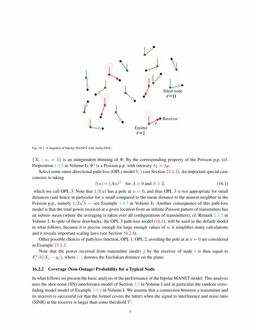
(3) {yi} denotes the location of the receiver for node Xi (we assume here that no two transmittershave the same receiver). We assume that the random vectors {Xi − yi} are i.i.d with |Xi −yi| = r; i.e. each receiver is at distance r from its transmitter (see Figure 16.1). There is nodifficulty extending what is described below to the case where these distances are independentand identically distributed random variables, independent of everything else.

(4) {Fi = (F ji : j)}where F ji denotes the virtual power emitted by node i (provided ei = 1) towardsreceiver yj . By virtual power F ji , we understand the product of the effective power of transmitteri and of the random fading from this node to receiver yj (cf. Remark 2.3.1 in Volume I). Therandom vectors {Fi} are assumed to be i.i.d. and the components (F ji , j) are assumed to beidentically distributed (distributed as a generic random variable (r.v.) denoted by F ) with mean1/µ assumed finite. In the case of constant effective transmission power 1/µ and Rayleigh fading,F is exponential with mean 1/µ (see Section 23.2.4). In this case, it is reasonable to assume thatthe components of (F ji : j) are independent, which is the default option in what follows. Thisis justified if the distance between two receivers is larger than the coherence distance of thewireless channel (cf. Section 23.3), which is a natural assumption here. Below, we also considernon-exponential cases which allow one to analyze other types of fading scenarios such as e.g.Rician or Nakagami (see Section 23.2.4) or simply the case without fading (when F ≡ 1/µ isdeterministic).

In addition, we consider a non-negative random variable W independent of Φ modeling the power of thethermal noise. A natural extension consists in considering a random field rather than a random variable.

Since we assume that Aloha is used, the set of nodes that transmit in the reference time slot Φ1 =

1The fact that all receivers are at the same distance from their transmitter is a simplification that will be relaxed in Chapter 16.

4

1e=

Emitter

e=0

Silent node

r

Receiver

Fig. 16.1 A snapshot of bipolar MANET with Aloha MAC.

{Xi : ei = 1} is an independent thinning of Φ; By the corresponding property of the Poisson p.p. (cf.Proposition 1.3.5 in Volume I), Φ1 is a Poisson p.p. with intensity λ1 = λp.

Select some omni-directional path-loss (OPL) model l(·) (see Section 23.1.2). An important special caseconsists in taking

l(u) = (Au)β for A > 0 and β > 2, (16.1)

which we call OPL 3. Note that 1/l(u) has a pole at u = 0, and thus OPL 3 is not appropriate for smalldistances (and hence in particular for u small compared to the mean distance to the nearest neighbor in thePoisson p.p., namely 1/2

√λ — see Example 1.4.7 in Volume I). Another consequence of this path-loss

model is that the total power received at a given location from an infinite Poisson pattern of transmitters hasan infinite mean (where the averaging is taken over all configurations of transmitters); cf. Remark 2.3.5 inVolume I. In spite of these drawbacks, the OPL 3 path-loss model (16.1), will be used as the default modelin what follows, because it is precise enough for large enough values of u, it simplifies many calculationsand it reveals important scaling laws (see Section 16.2.4).

Other possible choices of path-loss function, OPL 1, OPL 2, avoiding the pole at at u = 0 are consideredin Example 23.1.3.

Note that the power received from transmitter (node) j by the receiver of node i is then equal toF ji /l(|Xj − yi|), where | · | denotes the Euclidean distance on the plane.

16.2.2 Coverage (Non-Outage) Probability for a Typical Node

In what follows we present the basic analysis of the performance of the bipolar MANET model. This analysisuses the shot-noise (SN) interference model of Section 2.3 in Volume I and in particular the random cross-fading model model of Example 2.3.9 in Volume I. We assume that a connection between a transmitter andits receiver is successful (or that the formet covers the latter) when the signal to interference and noise ratio(SINR) at the receiver is larger than some threshold T :

5

Definition 16.2.1. Transmitter {Xi} covers its receiver yi in the reference time slot if

SINRi =F ii /l(|Xi − yi|)

W + I1i

≥ T , (16.2)

where the interference I1i is the SN associated with Φ1, namely, I1

i =∑

Xj∈eΦ1, j 6=i Fij/l(|Xj − yi|) and

where T is some SINR threshold.

The last condition might be required in practice for xi to be successfully received by yi due to the use of aparticular coding scheme associated with a given bit-rate (cf. Section 24.3.4). It is also called the non-outageor the capture condition depending on the framework.

Remark: Later, in Section 16.2.3, we shall also consider adaptive coding schemes in which the appropriatechoice of coding scheme is selected for each observed SINR level, which allows one to obtain a bit-rateclose to that given by Shannon’s law for all such SINR.

In what follows we focus on the probability that this property holds true for the typical node of theMANET, given it is a transmitter. This notion can be formalized using Palm theory for stationary markedpoint processes (cf. Section 2.1.2 in Volume I).

Denote by δi the indicator that (16.2) holds, namely, that location yi is covered by transmitterXi. We canconsider δi as a new mark of Xi. The marked point process Φ enriched with these marks is still stationary(cf. Definition 2.1.4 in Volume I). However, in contrast to the original marks ei, yi,Fi, given the points of Φ,the random variables {δi} are neither independent nor identically distributed. Indeed, the points of Φ lyingin dense clusters have a smaller probability of coverage than more isolated points due to interference; inaddition, because of the shot noise variables I1

i , the random variables {δi} are dependent.By probability of coverage of a typical node given it is a transmitter, we understand

P0{ δ0 = 1 | e0 = 1} = E0[δ0 | e0 = 1],

where P0 is the Palm probability associated to the (marked) stationary point process Φ and where δ0 is themark of the point X0 = 0 a.s. located at the origin 0 under P0. This Palm probability P0 is derived from theoriginal (stationary) probability P by the following relation (cf. Definition 2.1.5 in Volume I)

P0{ δ0 = 1 | e0 = 1} =1

λ1|B|E[∑

i

δi1(Xi ∈ B)],

where B is an arbitrary subset of the plane and |B| is its surface. Thus, knowing that λ1|B| is the expectednumber of transmitters inB, the typical node coverage probability is the mean number of transmitters whichcover their receivers in any given window B in which we observe our MANET. Note that this mean is basedon a double averaging: a mathematical expectation – over all possible realizations of the MANET and, foreach realization, a spatial averaging – over all nodes in B.

If the underlying point process is ergodic (as it is the case for our i.m. Poisson p.p. Φ) the typical nodecoverage probability can also be interpreted as a spatial average of the number of transmitters which covertheir receiver in almost every given realization of the MANET and large B (tending to the whole plane; cf.Proposition 1.6.10 in Volume I).

For a stationary i.m. Poisson p.p., the probability P0 can easily be constructed using Slivnyak’s theorem(cf. Theorem 1.4.5 in Volume I): under P0, the nodes of the Poisson MANET and their marks follow the

6

distribution Φ ∪ {(X0 = 0, e0, y0,F0)}, where Φ is the original stationary i.m. Poisson p.p. (i.e. that seenunder the original probability P) and (e0, y0,F0) is a new copy of the mark independent of everything elseand distributed like all other i.i.d. marks (ei, yi,Fi) of Φ under P. (cf. Remark 2.1.7 in Volume I).

Note that, under P0, the node at the origin (the typical node), is not necessarily a transmitter; e0 is equalto 1 or 0 with probability p and 1− p respectively.

Denote by pc(r, λ1, T ) = E0[δ0 | e0 = 1] the probability of coverage of the typical MANET node givenit is a transmitter. It follows from the above construction that this probability only depends on the densityof effective transmitters λ1 = λp, on the distance r and on the SINR threshold T ; it can be expressed usingthree independent generic random variables F, I1,W by the following formula:

pc(r, λ1, T ) = P0{F 00 > l(r)T (W + I1

0 ) | e0 = 1 } = P{F ≥ T l(r)(I1 +W ) } . (16.3)

Note also that this probability is equal to the one-point coverage probability p0(y0) in the GIW+M/GI SINR

cell model of Section 5.3.1 in Volume I associated with the Poisson p.p. intensity λ1. (see the meaningof this Kendall-like notation in Section 5.3 in Volume I). For this reason, our Aloha MANET model is ofthe GI

W+M/GI type, where the GI in the numerator indicates a general distribution for the virtual power ofthe signal F and where the M/GI in the denominator indicates that the SN interference is generated by aPoisson pattern of interferers (M), with a general distribution (G) for their virtual powers. Special cases ofdistributions marks are deterministic (D) and exponential (M). We recall that M/· denotes a SN model witha Poisson point process.

In what follows, we often use the following explicit formula for the Laplace transform of the genericshot-noise I1 =

∑Xj∈eΦ1 Fj/l(|Xj |), which is valid in the Poisson p.p. case whenever the random variables

Fj are independent copies of the generic fading variable F (cf. Corollary 2.3.8 in Volume I):

LI1(s) = E[e−I1s] = exp

{−λ12π

∞∫0

t(

1− LF (s/l(t)))

dt}, (16.4)

where LF is the Laplace transform of F . This can be derived from the formula for the Laplace functional ofthe Poisson p.p. (see Propositions 1.2.2 and 2.2.4 in Volume I).

16.2.2.1 Rayleigh Case

The next result bears on the Rayleigh fading case (F exponential with mean 1/µ). Using the independenceassumptions, it is easy to see that the right-hand side of (16.3) can be rewritten as

pc(r, λ) = pc(r, λ, T ) = E[e−µ(T l(r)(I1+W )

]= LI1(µT l(r))LW (µT l(r)) , (16.5)

where LW is the Laplace transform of W and where LI1 can be expressed as follows from (16.4) whenusing the fact that F is exponential:

LI1(s) = exp

−2πλ1

∞∫0

t

1 + µl(t)/sdt

. (16.6)

Using this observation, one immediately obtains (cf. also Proposition 5.3.3 and Example 5.3.4 in Volume I):

7

Proposition 16.2.2. For the MW+M/M bipolar model,

pc(r, λ1, T ) = LW (µT l(r)) exp{− 2πλ1

∞∫0

u

1 + l(u)/(T l(r))du}. (16.7)

In particular if W ≡ 0 and that the path-loss model (16.1) is used then

pc(r, λ1, T ) = exp(−λ1r2T 2/βK(β)) , (16.8)

where

K(β) =2πΓ(2/β)Γ(1− 2/β)

β=

2π2

β sin(2π/β). (16.9)

Example 16.2.3. The above result can be used in the following context: assume one wants to operate aMANET in a regime where each transmitter is guaranteed a SINR at least T with a probability larger than1− ε, where ε is a predefined quality of service, or equivalently, where the probability of outage is less thenε. Then, if the transmitter-receiver distance is r, the MAP p should be such that pc(r, λp, T ) = 1 − ε. Inparticular, assuming the path-loss setting (16.1), one should take

p = min(

1,− ln(1− ε)λr2T 2/βK(β)

)≈ min

(1,

ε

λr2T 2/βK(β)

). (16.10)

For example, for T = 10dB 2 and OPL 3 model with β = 4, r = 1, one should take p ≈ min (1, 0.064 ε/λ) .

16.2.2.2 General Fading

In what follows, we consider a GIW+M/GI bipolar Aloha MANET model. In this case one can get integral

representations for the probability of coverage on the basis of the results of Section 5.3.1 in Volume I.

Proposition 16.2.4. Consider a GIW+M/GI bipolar model with general fading variables F such that

• F has a finite first moment and admits a square integrable density;• Either I1 or W admit a density which is square integrable.

Then the probability of a successful transmission is equal to

pc(r, λ1, T ) =

∞∫−∞

LI1(2iπl(r)Ts)LW (2iπl(r)Ts)LF (−2iπs)− 1

2iπsds . (16.11)

2A positive real number x is 10 log10(x) dB.

8

Remark: Sufficient conditions for I1 to admit a density are given in Proposition 2.2.6 in Volume I. Roughlyspeaking these conditions require that F be non-null and that the path-loss function l be not constant in anyinterval. This is satisfied e.g. for the OPL 3 and OPL 2 model, but not for OPL 1 – see Example 23.1.3.Concerning the square integrability of the density, which is equivalent to the integrability of |LI1(is)|2(see (Feller 1971, p. 510) and also (2.20 in Volume I)), using (16.4), one can easily check that it is satisfiedfor the OPL 3 model provided P{F > 0} > 0. Moreover, under the same conditions |LI1(is)| is integrable(and so is |LI1(is)|/|s| for large |s|).

Proof. (of Proposition 16.2.4) By the independence of I1 andW in (16.3), the second assumption of Propo-sition 16.2.4 implies that I1 + W admits a density g(·) that is square integrable. The result then followsfrom

pc(r, λ1, T ) = P{ (I1 +W )T l(r) < F } ,

by the Plancherel-Parseval theorem; see e.g. (Bremaud 2002, Th. C3.3, p.157)) and for more details Corol-lary 12.2.2 in Volume I.

16.2.3 Shannon Throughput of a Typical Node

In Section 16.2.2 we assumed that a channel could be sustained if the SINR was above some fixed thresholdT , which corresponds to the case where some minimum bit rate is required (like in e.g. voice). In thissection we consider the situation where there is no minimal requirement on the bit rate T and where thelatter depends on the SINR through some Shannon like formula. This is possible with adaptive coding,where a coding with a high bit-rate is used if the SINR is high, whereas a coding with a low bit-rate is usedin case of lower SINR. We adopt the following definition.

Definition 16.2.5. We define the (Shannon) throughput (bit-rate) of the channel from transmitter Xi to itsreceiver yi to be

Ti = log(1 + SINRi) , (16.12)

where SINRi is as in Definition 16.2.1.

One can then ask about the throughput of a typical transmitter (or equivalently about the spatial average ofthe rate obtained by the transmitters), namely

τ = τ(r, λ1) = E0[T0 | e0 = 1] = E0[log(1 + SINR0) | e0 = 1]

and also about its Laplace transform

LT (s) = E0[e−sT0 | e0 = 1] = E0[(1 + SINR0)−s | e0 = 1] .

9

Let us now make the following simple observations:

τ(r, λ1) = E0[log(1 + SINR0) | e0 = 1]

=

∞∫0

P0{ log(1 + SINR0) > t | e0 = 1 } dt

=

∞∫0

P0{SINR0 > et − 1 | e0 = 1 } dt

=

∞∫0

pc(r, λ1, et − 1) dt =

∞∫0

pc(r, λ1, v)v + 1

dv (16.13)

and similarly

LT (s) = E0[(1 + SINR0)−s | e0 = 1]

= 1−1∫

0

pc(r, λ1, t−1/s − 1) dt = 1− s

∞∫0

pc(r, λ1, v)(1 + v)1+s

dv , (16.14)

provided P{SINR0 = T} = 0 for all T ≥ 0, which is true e.g. when F admits a density (cf. (16.3)). This,together with Propositions 16.2.2 and 16.2.4, lead to the following results:

Corollary 16.2.6. Under the assumptions of Proposition 16.2.2 (namely for the model with Rayleigh fad-ing) and for the OPL 3 path-loss model (16.1)

τ =β

2

∞∫0

e−λ1K(β)r2v vβ2−1

1 + vβ2

LW(µ(Ar)βvβ/2

)dv (16.15)

and

LT (s) =βs

2

∞∫0

(1− e−λ1K(β)r2vLW

(µ(Ar)βvβ/2

)) vβ2−1(

1 + vβ2

)1+s dv , (16.16)

where K(β) is defined in (16.9).

Corollary 16.2.7. Under the assumptions of Proposition 16.2.4 (namely in the model with general fadingF ),

τ =

∞∫0

∞∫−∞

LI1 (2iπvsl(r))LW (2iπvsl(r))LF (−2iπs)− 1

2iπs(1 + v)dsdv (16.17)

and

LT (s) = 1− s∞∫

0

∞∫−∞

LI1 (2iπvsl(r))LW (2iπvsl(r))LF (−2iπs)− 12iπs(1 + v)1+s

dsdv . (16.18)

Here is a direct application of the last results.

10

r = .25 r = .37 r = .5 r = .65 r = .75 r = .9 r = 1Rayleigh 1.52 .886 .480 .250 .166 .0930 .0648Erlang (8) 1.71 .942 .495 .242 .155 .0832 .0571

Table 16.1 Impact of the fading on the mean throughput τ for varying distance r. The Erlang distribution of order 8 mimics the no-fading case; weuse OPL3 3 with A = 1, β = 4 and Rayleigh (exponential) thermal noise W with mean 0.01.

Example 16.2.8. Table 16.1 shows how Rayleigh fading compares to the situation with no fading. TheOPL 3 model is assumed with A = 1 and β = 4. We assume W to be exponential with mean 0.01. We usethe formulas of the last corollaries; the Rayleigh case is with F exponential of parameter 1; to represent theno fading case within this framework we take F Erlang of high order (here 8) with the same mean 1 as theexponential. The reason for using Erlang rather than deterministic is that the latter does not satisfy the firsttechnical condition of Proposition 16.2.4. We see that the presence of fading is beneficial in the far-field,and detrimental in the near-field.

16.2.4 Scaling Properties

We show below that in the Poisson bipolar network model of Section 16.2.1, when using the OPL 3model (16.1) and when W = 0, some interesting scaling properties can be derived.

Denote by pc(r) = pc(r, 1, 1) the value of the probability of coverage calculated in this model withT ≡ 1, λ1 = 1,W ≡ 0 and with normalized virtual powers F ji = µF ji . Note that pc(r) does not depend onany parameter of the model other than the distribution of the normalized virtual power F .

Proposition 16.2.9. In the Poisson bipolar network model of Section 16.2.1 with path-loss model (16.1)and W = 0

pc(r, λ1, T ) = pc(rT 1/β√λ1) .

Proof. The Poisson point process Φ1 with intensity λ1 > 0 can be represented as {X ′i/√λ1 }, where Φ′ =

{X ′i} is Poisson with intensity 1 (cf. Example 1.3.12 in Volume I). Because of this, under (16.1), the Poissonshot-noise interference variable I1 admits the following representation: I1 = λ

β/21 I ′1, where I ′1 is defined

in the same manner as I1 but with respect to Φ′. Thus for W = 0,

pc(r, λ1, T ) = P(F ≥ T (Ar)βI1)

= P(µF ≥ µ(ArT 1/βλ

1/21 )βI ′1

)= pc(rT 1/β

√λ1 ) .

Remark 16.2.10. The scaling of the coverage probability presented in Proposition 16.2.9 is the first ofseveral examples of scaling in

√λ. Recall that this is also how the transport capacity scales in the well-

known Gupta and Kumar law. There are three fundamental ingredients for obtaining this scaling in thepresent context:

11

• the scale invariance property of the Poisson p.p. (cf. Example 1.3.12 in Volume I),• the power-law form of OPL 3,• the fact that thermal noise was neglected.

Note however the following important limitations concerning this scaling. First, when λ → ∞, the nodesare closer to each other and one may challenge the use of OPL 3 (the pole at the origin is not adequate forrepresenting the path loss on small distances). On the other hand, when λ → 0, the transmission distancesare very long; communications become noise limited and the assumption W = 0 may no longer be justified.

16.3 Spatial Performance Metrics

When trying to maximize the coverage probability pc(r, λ1, T ) or the throughput τ(r, λ1), one obtains de-generate maxima at r = 0. Assuming that our MANET features packets which have to reach some distantdestination nodes, a more meaningful optimization consists in maximizing some distance-based character-istics. In the coverage scenario, we for instance consider the mean progress made in a typical transmission:

prog(r, λ1, T ) = rE0[δ0] = rpc(r, λ1, T ) . (16.19)

Similarly, in the digital communication (or Shannon-throughput) scenario, we define the mean transport ofa typical transmission as

trans(r, λ1, T ) = rE0[T0] = rτ(r, λ1) . (16.20)

These characteristics might still not lead to pertinent optimizations of the MANET, as they are concernedwith one (typical) transmission. In particular, they are trivially maximized when p→ 0, when transmissionsare very efficient but very rare in the network. In fact, we need some network (social) performance metrics.

Definition 16.3.1. We call

• (spatial) density of successful transmissions, dsuc, the mean number of successful transmissionsper surface unit;• (spatial) density of progress, dprog, the mean number of meters progressed by all transmissions

taking place per surface unit;• (spatial) density of throughput, dthrou, the mean throughput per surface unit;• (spatial) density of transport, dtrans, the mean number of bit-meters transported per second and

per unit of surface.

The knowledge of pc(r, λ1, T ) or τ(r, λ1) allows one to estimate these spatial network performancemetrics. The link between individual and social characteristics is guaranteed by Campbell’s formula (cf. (2.9in Volume I)).

In what follows we make precise the meaning of the characteristics proposed in Definition 16.3.1 forPoisson bipolar MANETs.

The density of successful transmissions can formally be seen as the mean number of successful trans-missions in some arbitrary subset B of the plane:

dsuc(r, λ1, T ) =1|B|

E[∑

i

eiδi1(Xi ∈ B)].

12

By stationarity, the last quantity does not depend on the particular choice of set B. Let g(x, Φ) = 1(x ∈B)e0δ0. The right hand side of the above equation can be expressed as

1|B|

E[∫R2

g(x, Φ− x) Φ(dx)],

and by Campbell’s formula (2.9 in Volume I) is equal to

λ

|B|

∫R2

E0[g(x, Φ)] dx = λE0[e0δ0] ,

which gives the following result

dsuc(r, λ1, T ) = λ1pc(r, λ1, T ) = λppc(r, λp, T ). (16.21)

Similarly, the density of progress can be defined as the mean distance progressed by all transmissionstaking place in some arbitrary subset B of the plane

dprog(r, λ1, T ) =1|B|

E[∑

i

reiδi1(Xi ∈ B)]

= rλ1pc(r, λ1, T ) , (16.22)

by the same arguments as for (16.21).The spatial density of throughput is equal to

dthrou(r, λ1) =1|B|

E[∑

i

ei1(Xi ∈ B) log(1 + SINRi)]

= λ1τ(r, λ1) (16.23)

and the density of transport to

dtrans(r, λ1) =1|B|

E[∑

i

eir1(Xi ∈ B) log(1 + SINRi)]

= λ1rτ(r, λ1). (16.24)

In the following sections we focus on the optimization of the spatial performance of an Aloha MANET.

16.3.1 Optimization of the Density of Progress

16.3.1.1 Best MAP Given Some Transmission Distance

We already mentioned that a good tuning of p should find a compromise between the average number ofconcurrent transmissions per unit area and the probability that a given authorized transmission is successful.To find such a compromise, one ought to maximize the density of progress, or equivalently the density ofsuccessful transmissions, dsuc(r, λp, T ) = λp pc(r, λp, T ), w.r.t. p, for a given r and λ. This can be doneexplicitly for the Poisson bipolar network model with Rayleigh fading. For this we first optimize w.r.t. λassuming p fixed and then deduce from this the optimal MAP for some fixed λ.

Defineλmax = arg max

0≤λ<∞dsuc(r, λ, T ) ,

whenever such a value of λ exists and is unique. The following result follows from Proposition 16.2.2.

13

Proposition 16.3.2. Under the assumptions of Proposition 16.2.2 (namely for the MW+M/M model), if p = 1,

the unique maximum of the density of successful transmissions dsuc(r, λ, T ) is attained at

λmax =

2π

∞∫0

u

1 + l(u)/(T l(r))du

−1

,

and the maximal value is equal to

dsuc(r, λmax, T ) = e−1λmax LW (µT l(r)) .

In particular, assuming W ≡ 0 and OPL 3 model (16.1)

λmax =1

K(β)r2T 2/β, (16.25)

dsuc(r, λmax, T ) =1

eK(β)r2T 2/β. (16.26)

with K(β) defined in (16.9).

Proof. The result follows from (16.7) by differentiation of the function λpc(r, λ, T ) with respect to λ.

The above result yields the following corollary concerning the tuning of the MAC parameter when λ is fixed.

Corollary 16.3.3. Under assumptions of Proposition 16.2.2 with given r, the value of the MAP p that max-imizes the density of successful transmissions is

pmax = min(1, λmax/λ) .

In order to extend our observations to general fading (or equivalently to a general distribution for vir-tual power), let us assume that W = 0 and let us adopt model OPL 3. Then, for Rayleigh fading, usingLemma 16.2.9, we can easily show that λmax and dsuc(r, λmax) exhibit, up to some constant, the same de-pendence on the model parameters (namely r, T and µ) as that given in (16.25) and (16.26).

Proposition 16.3.4. In the GI0+M/GI bipolar model with OPL 3 and W = 0,

λmax =const1r2T 2/β

, and dsuc(r, λmax) =const2r2T 2/β

, (16.27)

where the constants const1 and const2 do not depend on r, T, µ, provided λmax is well defined.

Proof. Assume that λmax is well defined. 3 By Lemma 16.2.9, const1 = arg maxλ≥0{λpc(√λ)} and

const2 = maxλ≥0{λpc(√λ)}.

14

0

0.005

0.01

0.015

0.02

0.025

0.03

0 0.05 0.1 0.15 0.2

De

nsity o

f su

cce

ssfu

l tr

an

sm

issio

ns dsuc

MAP p

RayleighRician q=0.5Rician q=0.9

Fig. 16.2 Density of successful transmissions dsuc for Aloha in function of p in the Rayleigh and the Rician (with q = 1/2 and q = .9) fadingcases; λ = r = 1, W = 0, and T = 10dB; we use OPL 3 with A = 1 and β = 4.

Example 16.3.5 (Rayleigh versus Rician fading). Figure 16.2 compares the density of success forRayleigh and Rician fading. For this, we use the representations of Propositions 16.2.2 and Proposition16.2.4, respectively. In the Rayleigh case, F is exponential with mean 1. In the Rician case F = q+(1−q)F ′,with 0 ≤ q ≤ 1, where F ′ is exponential with mean 1 and q represents the part of the energy received on theline-of-sight. The density of success is plotted in function of p. We again observe that higher variances arebeneficial for high densities of transmitters (which is here equivalent to the far field case) and detrimental forlow densities. However here, in each case, there is an optimal MAP, and when properly optimized, SpatialAloha does better for lower variances (i.e. for Rician fading with higher q).

16.3.1.2 *General Definition of λmax

In this section, we show that under some mild conditions, λmax is well defined and not degenerate (i.e.0 < λmax < ∞) for a general GI

W+M/GI model. Assume T > 0. Note that dsuc(r, 0, T ) = 0; so under somenatural non-degeneracy assumptions, the maximum is certainly not attained at λ = 0.

Proposition 16.3.6. Consider the GIW+M/GI bipolar model with p = 1 and general fading with a finite mean.

Assume that l(r) > 0 and is such that the generic SN I(λ) =∑

Xj∈eΦ Fj/l(|Xj |) admits a density for allλ > 0. Then

(1) If P{F > 0 } > 0, then pc(r, x, T ) (and so dsuc(r, x, T )) is continuous in x, so that the maxi-mum of the function x→ dsuc(r, x, T ) in the interval [0, λ] is attained for some 0 < λmax ≤ λ;

(2) If for all a > 0, the following modified SN:

I ′(λ) =∑Xj∈eΦ

1(|Xj | > a)Fj/l(|Xj |)

3The question of the definition of λmax is addressed in § 16.3.1.2.

15

has finite mean for all λ > 0, then limx→∞ dsuc(r, x, T ) = 0 and consequently, for sufficientlylarge λ, this maximum is attained for some λmax < λ.

The statement of the last proposition means that for a sufficiently large density of nodes λ, a nontrivialMAP 0 < pmax < 1 equal to pmax = λmax/λ optimizes the density of successful transmissions.

Proof. (of Proposition 16.3.6) Recall that pc(r, λ, T ) = P{ I(λ) ≤ F/(l(r)T−W ) }, where the dependenceof the SN variable I(λ) = I1 = I (note that p = 1) on the intensity of the Poisson p.p. was made explicit.By the thinning property of the Poisson p.p. (stated in Proposition 1.3.5 in Volume I) we can split the SNvariable into two independent Poisson SN terms I(λ+ ε) = I(λ) + I(ε). Moreover, we can do this in sucha way that I(ε), which is finite by assumption, almost surely converges to 0 when ε→ 0. Consequently,

0 ≤ pc(r, λ, T )− pc(r, λ+ ε, T ) = P{ F

l(r)T −W− I(ε) < I(λ) ≤ F

l(r)T −W

},

andlimε→0

(pc(r, λ, T )− pc(r, λ+ ε, T )

)= P

{I(λ) =

F

l(r)T −W

}= 0 ,

where the last equation is due to the fact that I(λ) is independent of F,W and admits a density. Splitting thePoisson p.p. of intensity λ into two Poisson p.p.s with intensity λ− ε and ε respectively, and considering theassociated SN variables I(λ− ε) and I(ε), with I(λ) defined as their sum, one can show in a similar mannerthat limε→0 pc(r, λ− ε, T )− pc(r, λ, T ) = 0. This concludes the proof of the first part of the proposition.

We now prove the second part. Let G(s) = P{F ≥ s }. Take ε > 0 and such that ε < E[I ′(1)] =I′(1) <∞. By independence we have

dsuc(r, λ, T ) = λpc(r, λ, T ) ≤ λE[P{F ≥ I ′(λ)T l(r)|I ′(λ)

}]≤ J1 + J2 ,

where

J1 = E[ λ

I ′(λ)1(I ′(λ) ≥ λ(I ′(1)− ε)

)I ′(λ)G

(I ′(λ)T l(r)

)]J2 = λE

[1(I ′(λ) < λ(I ′(1)− ε)

)].

Since E[F ] =∫∞

0 G(s) ds < ∞, I ′(λ)G(I ′(λ)T l(r)

)is uniformly bounded in I ′(λ) and

I ′(λ)G(I ′(λ)T l(r)

)→ 0 when I ′(λ) → ∞. Moreover, one can construct a probability space such that

I ′(λ) → ∞ almost surely as λ → ∞. Thus, by Lebesgue’s dominated convergence theorem, we havelimλ→∞ J1 = 0.

For J2 and t > 0 we have

J2 ≤ λP0{ e−tI′(λ) ≥ e−λt(I′(1)−ε) }

≤ λE0[e−tI

′(λ)+λt(I′(1)−ε)]

= λ exp{λ(t(I ′(1)− ε)− 2π

∞∫a

s(1− LF (t/l(s))

)ds)}

.

Note that the derivative of t(I ′(1)− ε)− 2π∫∞a s

(1− LF (t/l(s))

)ds with respect to t at t = 0 is equal to

I′(1)− ε− I ′(1) < 0. Thus, for some small t > 0, J2 ≤ λe−λC for some constant C > 0. This shows that

limλ→∞ J2 = 0, which concludes the proof.

16

16.3.1.3 Best Transmission Distance Given Some Transmitter Density

Assume now some given intensity λ1 of transmitters. We look for the distance r which maximizes the meandensity of progress, or equivalently the mean progress prog(r, λ1, T ) = r pc(r, λ1, T ). We denote by

rmax = rmax(λ) = arg maxr≥0

prog(r, λ, T )

the best transmission distance for the density of transmitters λ whenever such a value exists and is unique.Let

ρ = ρ(λ) = prog(rmax(λ), λ, T )

be the optimal mean progress.

Proposition 16.3.7. In the GI0+M/GI bipolar model with OPL 3 function and W = 0,

rmax(λ) =const3T 1/β

√λ, and ρ(λ) =

const4T 1/β

√λ, (16.28)

where the constants const3 and const4 do not depend on R, T, µ, provided rmax is well defined. If F isexponential (i.e. for Rayleigh fading) and l(r) given by (16.1) then const3 = 1/

√2K(β) and const4 =

1/√

2eK(β).

Proof. The result for general fading follows from Lemma 16.2.9. The constants for the exponential case canbe evaluated by (16.8).

Remark 16.3.8. We see that the optimal distance rmax(λ) from transmitter to receiver is of the order of thedistance to the nearest neighbor of the transmitter, namely 1/(2

√λ), when λ → ∞. Notice also that for

Rayleigh fading and l(r) given by (16.1) we have the general relation:

2r2λmax(r) = rmax(λ)2λ. (16.29)

As before, one can show that for a general model, under some regularity conditions, prog(r, λ, T ) iscontinuous in r and that the maximal mean progress is attained for some positive and finite r. We skip thesetechnicalities.

16.3.1.4 Degeneracy of Two Step Optimization

Assume for simplicity a W = 0 and OPL 3 path-loss (16.1). In Section 16.3.1.1, we found that for fixed r,the optimal density of successful transmissions dsuc is attained when the density of transmitters is equal toλ1 = λmax = const1/(r2T 2/β). It is now natural to look for the distance r maximizing the mean progressfor the network with this optimal density of transmitters. But by Proposition 16.3.4

supr≥0

prog(r, λmax, T ) = supr≥0

r pc(r, λmax, T )

= supr≥0

rdsuc(r, λmax, T )

λmax

= supr≥0

rconst2const1

=∞ ,

17

and thus the optimal choice of r consists in taking r = ∞, and consequently λmax = 0. From a practicalpoint of view, this is not of course an acceptable answer. The fact that the optimal value is r =∞ might bea consequence of the fact that we took W = 0. But even if this is the case, the above observation suggeststhat for a small W > 0, a (possibly) finite optimal value of r would be too large from a practical point ofview.

In a network-perspective, one might better optimize a more “social” characteristic of the MANET likee.g. the density of progress dprog = λrpc(r, λ, T ) first in λ and then in r. However in this case one obtainsthe opposite degenerate answer:

supr≥0

dprog(r, λmax, T ) = supr≥0

r dsuc(r, λmax, T ) = supr≥0

rconst2r2T 2/β

= 0 ,

which is attained for r = 0 and λmax =∞.The above analysis shows that a better receiver model is needed to study the joint optimization in the

transmission distance and in λ. We propose such models in Chapter 17, where the receivers are no longersampled as independent marks of the Poisson p.p. of potential transmitters, but belong to the point process ofpotential transmitters; more precisely, they are chosen among the nodes which are silenced by Aloha duringthe considered time slot. As we shall see in Section 17.4 these degeneracies may then vanish.

16.3.2 Optimization of the Density of Transport

16.3.2.1 Best MAP Given Some Transmission Distance

Defineλtransmax = arg max

0≤λ<∞dtrans(r, λ)

whenever such a value of λ exists and is unique. We have the following result.

Proposition 16.3.9. In the M0+M/M bipolar model with OPL 3 and W = 0, the unique maximum λtransmax of

the density of transport dtrans(r, λ) is attained at

λtransmax =x∗(β)r2K(β)

, (16.30)

where x∗(β) is the unique solution of the integral equation∞∫

0

e−xvvβ2−1

1 + vβ2

dv = x

∞∫0

e−xvvβ2

1 + vβ2

dv . (16.31)

Proof. One obtains this characterization by differentiating (16.15) w.r.t. λ1.

Example 16.3.10. Consider the following model: r = 1, fading is Rayleigh with parameter µ = 1; at-tenuation is OPL 3 with A = 1 and β = 4. One finds a unique positive solution to (16.31) which givesλtransmax ≈ 0.157. The associated mean throughput per node is τ(r, λtransmax ) ≈ 0.898. If one defines T ∗ by theShannon-like formula τ(r, λtransmax ) = log(1 + T ∗), one finds T ∗ ≈ 0.8635, which is a much lower SINRtarget than what is usually retained within this setting.

18

16.3.2.2 Best Transmission Distance Given a Density of Transmitters

Assume now some given intensity λ1 = λp of transmitters. We look for the distance r which maximizes themean density of transport, or equivalently the mean throughput τ(r, λ1). We denote by

rtransmax = rtransmax (λ) = arg maxr≥0

rτ(r, λ)

the best transmission distance for this criterion, whenever such a value of r exists and is unique.

Proposition 16.3.11. In the M0+M/M bipolar model with OPL 3, the unique maximum of the density of trans-

port dtrans(r, λ) is attained at

rtransmax =

√y∗(β)λK(β)

, (16.32)

where y∗(β) is the unique solution of the integral equation

∞∫0

e−yvvβ2−1

1 + vβ2

dv = 2y

∞∫0

e−yvvβ2

1 + vβ2

dv . (16.33)

Proof. One obtains this characterization by differentiating (16.15) w.r.t. r.

We do not pursue this line of thought any further. Let us nevertheless point out that the last results canbe extended to more general fading models and also that the same degeneracies as those mentioned abovetake place.

16.3.3 Spatial Reuse in Optimized Poisson MANETs

In wireless networks, the MAC algorithm is supposed to prevent simultaneous neighboring transmissionsfrom occurring, as often as possible, since such transmissions are likely to produce collisions. Some MACprotocols (as e.g. CSMA considered in Section 18.1) create exclusion zones to protect scheduled transmis-sions. Aloha creates a random exclusion disc around each transmitter. By this we mean that for an arbitraryradius there is some non-null probability that all the nodes in the disk with this radius do not transmit at agiven time slot.

Definition 16.3.12. We define the mean exclusion radius as the mean distance from a typical transmitter toits nearest concurrent transmitter

Rexcl = E0[mini 6=0{|Xi| : ei = 1}

].

19

Proposition 16.3.13. For the GIW+M/GI bipolar model, we have

Rexcl = Rexcl(λ1) =1

2√λ1

=1

2√λp

. (16.34)

Proof. The probability that the distance from the origin to the nearest point in the Poisson p.p. Φ1 of intensityλ1 = λp is larger than s is equal to e−λ1πs2 (cf. Example 1.4.7 in Volume I). Thus we have Rexcl =∫∞

0 e−λ1πs2 ds.

Here are two questions pertaining to an optimized scenario and which can be answered using the resultsof the previous sections:

• If r is given and p is optimized, how does the resulting Rexcl compare to r?• If λ is given and r is optimized, how does the resulting r compare to Rexcl?

We address these questions in a unified way using a notion of spatial reuse analogous to the concept ofspectral reuse used in cellular networks.

Definition 16.3.14. The spatial reuse factor of the bipolar Aloha MANET is the ratio of the distance rbetween the transmitter and the receiver and the mean exclusion radius Rexcl.

So if the spatial density of transmitters in this Aloha MANET is λ1, then

Sreuse = Sreuse(λ1, r) =r

Rexcl= 2r

√λ1. (16.35)

Here are a few illustrations.

Example 16.3.15. Consider the GIW+M/GI bipolar model of Section 16.2.1. Assume that the path-loss model

is OPL 3 and thatW = 0. Assume the fixed coding scenario of Section 16.2.2 i.e., the success of a transmis-sion requires a SINR larger than or equal to T . We deduce from Proposition 16.3.4 that the spatial intensityof transmitters that maximizes the density of successful transmissions is λmax = const1/(r2T 2/β). Henceby (16.34)

Rexcl(λmax) =1

2√λmax

= rT 1/β

2√

const1, (16.36)

so that at the optimum, the spatial reuse

Sreuse =2√

const1T 1/β

, (16.37)

is independent of r. For example, for β = 4 and Rayleigh fading, we can use the fact that const1 = 1/K(β)to evaluate the last expressions. For a SINR target of T = 10dB, Rexcl(λmax) ≈ 1.976r. EquivalentlySreuse ≈ 0.506. In order to have a spatial reuse larger than 1, one needs a SINR target less than

(2√

2/π)4

=0.657, that is less than -1.82 dB.

20

Example 16.3.16. Consider the Poisson bipolar network model of Section 16.2.1 with general fading, path-loss model (16.1) andW = 0 and target SINR T . Assume that the spatial density of transmitters is fixed andequal to λ. Let rmax(λ) denote the transmitter-receiver distance which maximizes the mean progress. We getfrom Proposition 16.3.7 that at the optimum r,

Sreuse =const32T 1/β

, (16.38)

for all values of λ. For β = 4 and Rayleigh fading, if we pick a SINR target of 10 dB, then Sreuse ≈ 0.358only. Similarly, Sreuse > 1 iff T < (2/K(β))β/2. For β = 4, this is iff T < 0.164 or equivalently T lessthan -7.84 dB.

Example 16.3.17. Assume the Poisson bipolar network model of Section 16.2.1 with Rayleigh fading,path-loss model (16.1) and W = 0. Consider the optimal coding scenario with Shannon throughput ofSection 16.2.3. The distance between transmitter and receiver is r. We deduce from Proposition 16.3.9 thatin terms of density of transport, the best organization of the MANET is that where the spatial intensity oftransmitters is λtransmax = x(β)/r2K(β). Hence, at the optimum,

Rexcl = r12

√K(β)x∗(β)

, (16.39)

so that

Sreuse = 2

√x∗(β)K(β)

, (16.40)

a quantity that again does not depend on r. For β = 4, one gets x∗(β) ≈ 0.771, so that Rexcl ≈ 1.27r andSreuse ≈ 0.790.

Example 16.3.18. Consider the same scenario as in the last example but assume now that the intensity oftransmitter is λ fixed. Proposition 16.3.11 shows that in order to maximize the mean throughput, in theoptimal scenario, the transmitter-receivers distance rtransmax is such that

Sreuse = 2

√y∗(β)K(β)

. (16.41)

For β = 4, y∗(β) ≈ 0.122 and Sreuse ≈ 0.314.

16.4 Opportunistic Aloha

In the basic Spatial Aloha scheme, each node tosses a coin to access the medium independently of thefading variables. It is clear that something more clever can be done by combining the random selection oftransmitters with the occurrence of good channel conditions. The general idea of opportunistic Aloha is toselect the nodes with the channel fading larger than a certain threshold as transmitters in the reference timeslot. This threshold may be deterministic or random (we assume fading variables to be observable whichis needed for this scheme to be implementable; for more details on implementation issues see (Baccelli,Blaszczyszyn, and Muhlethaler 2009a)).

21

16.4.1 Model Definition

More precisely, in a Poisson MANET, opportunistic Aloha with random MAC threshold can be describedby an i.m. Poisson p.p. Φ = {(Xi, θi, yi,Fi)}, where {(Xi, yi,Fi)} is as described in items (1)–(4) on theenumerated list in Section 16.2, with item (2) replaced by:

(2’) The medium access indicator ei of node i (ei = 1 if node i is allowed to transmit and 0 otherwise)is the following function of the virtual power F ii : ei = 1(F ii > θi), where {θi} are new randomi.i.d. marks, with a generic mark denoted by θ. Special cases of interest are

– that where θ is constant,

– that where θ is exponential with parameter ν.

In this latter case one can obtain a closed-form expression for the coverage probability.

We still assume that for each i, the components of (F ji , j) are i.i.d. Note that {ei} are again i.i.d. marks ofthe point process Φ (which of course depend on the marks {θi, F ii }).

In what follows, we also assume that for each i, the coordinates of (F ji , j) are i.i.d. (cf. assumption (4)of the plain Aloha model of Section 16.2).

The set of transmitters is hence a Poisson p.p. Φ1 (different from that in Section 16.2) with intensityλP(F > θ) (where F is a typical F ii and θ a typical θi, with (F, θ) independent). Thus in order to compareopportunistic Aloha to the plain Aloha described in Section 16.2, one can take p = P{F > θ }, where p isthe MAP of plain Aloha, which guarantees the same density of (selected) transmitters at a given time slot.

16.4.2 Coverage Probability

Note that the virtual power emitted by any node to its receiver, given it is selected by opportunistic Aloha(i.e. given ei = 1) has for law the distribution of F conditional on F > θ. Below, we denote by Fθ a randomvariable with this law.

By the independence of (F ji , j), the virtual powers F ji , j 6= i, toward other receivers are still distributedas F . Consequently, the interference I1

i experienced at any receiver has exactly the same distribution as inplain Aloha. Hence, the probability for a typical transmitter to cover its receiver can be expressed by thefollowing three independent generic random variables

pc(r, λ1, T ) = P{Fθ > Tl(r)(I1 +W ) } , (16.42)

where I1 is the generic SN generated by Poisson p.p. with intensity λ1 = P{F > θ}λ and (non-conditioned)fading variables Fj (as in (16.3)). Using the Kendall-like notation of Section 5.3 in Volume I, we can seepc(r, λ1, T ) as the coverage probability in some GI1

W+M/GI2model in which the distribution of interfering

virtual powers (GI2) is different from that of the useful signal (GI1).

16.4.2.1 Rayleigh Fading and Exponential Threshold Case

We begin our analysis of opportunistic Aloha by a comparison of pc(r, λ1, T ) and pc(r, λ1, T ) of plainAloha when all parameters (T , W , r, etc.) are the same. To get more insight we assume first Rayleighfading. In this case, F is exponential with parameter µ and since θ is independent of F , by the lack ofmemory property of the exponential variable, given that F > θ, the variables θ and F − θ are independent.Moreover, the conditional distribution of F − θ given F > θ is also exponential with parameter µ. Denote

22

by θ the conditional law of θ given that F > θ. Consequently in the Rayleigh fading case (16.42) can berewritten as

pc(r, λ1, T ) = E[e−µ(T l(r)(I

1+W )−eθ)+], (16.43)

where I1,W, θ are independent random variables with distributions described above and a+ = max(a, 0).Comparing (16.43) to the middle expression in (16.5) it is clear that the opportunistic scheme does betterthan plain Aloha with MAP p such that p = P(F > θ) = E

(e−µθ

)= Lθ(µ). This follows from the

fact that the intensity of transmitters is the same in both cases, which implies that the laws of interferencecoincide in both formulas.

In order to evaluate how much better opportunistic Aloha does in the Rayleigh case, we now focus onthe case when θ is exponential (of parameter ν). Note that in this case, θ is also exponential of parameterµ+ ν. This is thus a M1

W+M/M2model.

Proposition 16.4.1. Assume the Poisson bipolar network model of Section 16.2.1 with opportunistic AlohaMAC given by (2’) in Section 16.4.1. Assume Rayleigh fading (exponential F with parameter µ) and expo-nential distribution of θ with parameter ν. Then

pc(r, λ1, T ) =µ+ ν

νLI1(µT l(r))LW (µT l(r))− µ

νLI1((µ+ ν)T l(r))LW ((µ+ ν)T l(r)) ,

where LI1 is given by (16.6) with λ1 = λν/(µ + ν). If moreover W ≡ 0 and the OPL 3 model (16.1) isassumed, then

pc(r, λ1, ν) =µ+ ν

νexp{−λ1T

2/βr2K(β)} − µ

νexp{−λ1

((µ+ ν)T

µ

)2/β

r2K(β)},

with λ1 as above.

Proof. Note that Φ1 is a Poisson p.p. of intensity λν/(ν + µ) and θ is exponential of parameter µ + ν.Using (16.43) we have hence

pc(r, λ1, T )

= E[ T l(r)(I1+W )∫

0

(µ+ ν)e−(µ+ν)xe−µ(T l(r)(I1+W )−x)dx

]+ E

[ ∞∫T l(r)(I1+W )

(µ+ ν)e−(µ+ν)xdx]

=µ+ ν

νE[e−µT l(r)(I1+W ) − e−(µ+ν)T l(r)(I1+W )

]+ E

[e−(µ+ν)T l(r)(I1+W )

],

which completes the proof.

Note that, as expected, when letting ν tend to infinity, under mild conditions, the first expression of the lastproposition tends to LI1(µT l(r))LW (µT l(r)), namely the formula (16.7) of plain Aloha with λ1 = λ orequivalently p = 1.

16.4.2.2 General Case

For a general fading and distribution of θ (for instance deterministic θ, in which case obviously θ = θ), thefollowing result can be proved along the same lines as Proposition 16.2.4.

23

Proposition 16.4.2. Assume the Poisson bipolar network model of Section 16.2.1 with opportunistic AlohaMAC given by (2’) in Section 16.4.1 for some general distribution of F and θ. Take the same assumptionsas in Proposition 16.2.4 except that the condition on F is replaced by the following one

• E[Fθ] <∞ and Fθ admits a square integrable density.

Then

pc(r, λ1, T ) =

∞∫−∞

LI1 (2iπl(r)Ts)LW (2iπl(r)Ts)LFθ(−2iπs)− 1

2iπsds . (16.44)

Proof. It follows immediately from Equation (16.42) and Corollary 12.2.2 in Volume I.

In the case of Rayleigh fading and deterministic θ, the last theorem can be used since Fθ is then theconvolution of a deterministic distribution (with mean θ) and an exponential one (with parameter µ); thissatisfies the assumptions of the proposition. In this case, LFθ(s) = e−sθ µ

µ+s . Obviously it can also be usedwhen θ is exponentially distributed with intensity ν. In particular, for Rayleigh fading, we have LFθ(s) =µ+νµ+ν+s

µµ+s .

Example 16.4.3. Assume Rayleigh fading. In Figure 16.3 we plot the density of successful transmissionsdsuc in function of the parameter ν for three different scenarios:

(1) Opportunistic Aloha with a deterministic threshold θ with value 1/ν, where dsuc =λ1pc(r, λ1, ν), with λ1 = λe−

µν and pc(r, λ1, ν) given by Proposition 16.4.2;

(2) Opportunistic Aloha with a random exponential threshold with parameter ν, where dsuc =λ1pc(r, λ1, ν), with λ1 = λν

µ+ν and pc(r, λ, ν) given by Proposition 16.4.1;(3) Plain Aloha where dsuc = 1/(eK(β)r2T 2/β) is the optimal density of successful transmissions

as obtained in Proposition 16.3.2 (this is of course a constant in ν).

In the particular case considered in this figure, the density of transmitters covering their target receiver isapprox. 56% larger in the optimal opportunistic scheme with exponential threshold than in plain Aloha and134% larger in the deterministic case.

It may look surprising that the curves for the random exponential and the deterministic threshold cases(1 and 2 above) differ so much. One should bear in mind the fact that the two associated MAPs are quitedifferent: p = ν

µ+ν in the former case and p = e−µν in the latter.

Example 16.4.4 (Rayleigh versus Rician fading). (Example 16.3.5 continued).Figure 16.4 compares the density of success of opportunistic Aloha for Rayleigh and Rician (q = 1/2)

fading. (The Rician case with q = .9 has thresholds θ larger than .9 and leads to very small densitiesof success; it is not displayed). The two curves are based on Proposition 16.4.2. Note first that for the twoconsidered cases the density of transmitters are quite different: (exp(−θ) in the Rayleigh case and exp(−2θ)in the Rician case, for θ > 1/2), which explain why the shapes of the curves are so different. Here, we see

24

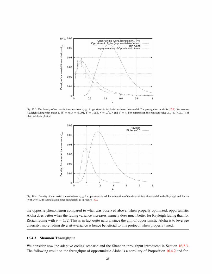
0

0.01

0.02

0.03

0.04

0.05

0.06

0 0.2 0.4 0.6 0.8 1

De

nsity o

f su

cce

ssfu

ll tr

an

sm

issio

ns dsuc

ν

10-3

xOpportunistic Aloha (constant θ = 1/ν)

Opportunistic Aloha (exponential θ of rate ν)Plain Aloha

Implementation of Opportunistic Aloha

Fig. 16.3 The density of successful transmissions dsuc of opportunistic Aloha for various choices of θ. The propagation model is (16.1). We assumeRayleigh fading with mean 1, W = 0, λ = 0.001, T = 10dB, r =

p1/λ and β = 4. For comparison the constant value λmaxpc(r, λmax) of

plain Aloha is plotted.

0

0.01

0.02

0.03

0.04

0.05

0.06

0 1 2 3 4 5 6

De

nsity o

f su

cce

ssfu

l tr

an

sm

issio

ns dsuc

θ

RayleighRician q=0.5

Fig. 16.4 Density of successful transmissions dsuc for opportunistic Aloha in function of the deterministic threshold θ in the Rayleigh and Rician(with q = 1/2) fading cases; other parameters as in Figure 16.2.

the opposite phenomenon compared to what was observed above: when properly optimized, opportunisticAloha does better when the fading variance increases, namely does much better for Rayleigh fading than forRician fading with q = 1/2. This is in fact quite natural since the aim of opportunistic Aloha is to leveragediversity: more fading diversity/variance is hence beneficial to this protocol when properly tuned.

16.4.3 Shannon Throughput

We consider now the adaptive coding scenario and the Shannon throughput introduced in Section 16.2.3.The following result on the throughput of opportunistic Aloha is a corollary of Proposition 16.4.2 and for-

25

0

0.05

0.1

0.15

0.2

0.25

0.3

0 0.2 0.4 0.6 0.8 1

De

nsity o

f th

rou

gh

pu

t dthrou

ν

10-3

xOpportunistic Aloha (constant θ = 1/ν)

Opportunistic Aloha (exponential θ of rate ν)Plain Aloha p=ν

Fig. 16.5 The density of throughput of opportunistic Aloha as a function of its parameter ν and that of plain Aloha. Assumptions are as inFigure 16.3.

mula (16.13).

Corollary 16.4.5. Under the assumptions of Proposition 16.4.2, the mean Shannon throughput of the typicaltransmitting node is

τ =

∞∫0

∞∫−∞

LI1 (2iπvsl(r))LW (2iπvsl(r))LFθ(−2iπs)− 1

2iπs(1 + v)dsdv . (16.45)

Since the assumptions of the last result hold in both deterministic and exponential θ case for Rayleigh fading,we can use (16.45) to evaluate the density of throughput in both cases.

Example 16.4.6. Figure 16.5 plots the density of throughput dthrou for Rayleigh fading and the same threecases of θ as in Example 16.4.3. In the particular case considered in this figure, the density of throughput isapprox. 48% larger in the optimal opportunistic scheme with exponential threshold than in plain Aloha and93% larger in the deterministic case.

Remark: The deterministic threshold case seems to always outperform the exponential threshold case whenboth are tuned optimally.

16.5 Conclusion

The two main assumptions of the chapter are that time is slotted and that the receivers are at some predefinedfrom their transmitters. The last assumption is relaxed in the next chapter. Let us conclude with a fewcomments on how to relax the slotted time assumption.

Time–slots are required in e.g. TDMA (Time Division Multiple Access) and one of the well known ad-vantages of Aloha is that it does not require slotted time. In order to model non-slotted Aloha, one has to

26

take into account the fact that interference (and thus SINR) can vary during a given transmission as someother transmissions may start or terminate. A more detailed packet reception model is hence needed. Forexample, if one assumes a coding with sufficient interleaving, then one can consider that it is the aver-aged SINR, where the averaging is over the whole packet reception period, that determines the success ofreception. In this case a mathematical analysis of non-slotted Aloha is possible e.g. along the lines pre-sented in (Błaszczyszyn and Radunovic 2007; Błaszczyszyn and Radunovic 2008); see also a forthcomingpaper (Błaszczyszyn and Muhlethaler 2010).

27

17Receiver Selection in Spatial Aloha

17.1 Introduction

In this chapter, we consider a few possible scenarios where the receiver of a given transmitter is not necessar-ily at distance r, as in the Poisson bipolar model (cf. Section 16.2.1) considered so far. In a MANET, somerouting algorithm (cf. Section 25.3.1.2) specifies the receivers(s) (relay node(s)) of each given transmitter.The joint analysis and the joint design of MAC and routing are difficult tasks even if we assume the simplestMAC (Aloha). We shall come back to such cross-layer routing schemes in Chapter 22. In this chapter, wemake a first step in this direction by proposing receiver models based on simplifying assumptions on therouting layer. Specifically, we assume one of the following routing principles:

• Each transmitter selects its receiver as close by as possible. We saw in Section 16.3.1.4, in oneof the two-step optimizations (with respect to λ and then r), that it is in some sense best for atransmitter to select his receiver as close by as possible. This justifies the class of routing modelswhich is considered in Section 17.2 and which consist in making as small as possible hops.• Each transmitter targets all available (potential) receivers. This assumption, of interest in multi-

cast scenarios, is considered in Section 17.3.• Each transmitter targets the most distant successful receiver. In this scenario, as in the previous

one, each transmitter targets all available receivers; however, some selection policy is appliedamong the nodes which successfully receive the packet. One selects the node optimizing thepacket progress in a given direction as the relay node. All other nodes discard the packet (this isnot a broadcast scheme). This opportunistic scenario, in which no specific receiver is prescribedin advance by the routing algorithm, and where one selects the best hop at the given time step, isconsidered in Section 17.4.

The above routing principles are considered in conjunction with the following models regarding receiverlocations:

• The independent receiver model, where the potential receivers form a stationary p.p. Φ0 withintensity λ0, independent of the transmitter p.p. Φ. This model, considered in Section 17.2.1,

29

corresponds to the situation where the nodes of Φ transmit to randomly located nodes (accesspoints or relay stations) which are external to the MANET. Several further specifications of thismodel are of interest. For example:

– The independent Poisson receiver model, where Φ0 is some homogeneous Poisson p.p.

– The independent honeycomb receiver model, where Φ0 is some stationary hexagonalgrid; cf. Example 4.2.5 in Volume I.

– The independent Poisson + periodic receiver model, where Φ0 is the superposition oftwo independent p.p.s, a Poisson p.p. of intensity λ0 − ε > 0, and a stationary grid (e.g.the hexagonal one) of intensity ε > 0. The presence of the periodic stations providesan upper-bound on the distance to the nearest neighbor, which can be arbitrarily largein the pure Poisson receiver model. The advantages of this solution will be discussed inSection 17.5.

• The MANET receiver model, where the transmitters of the MANET Φ choose their receivers inthe original set Φ of nodes of the MANET. Two scenarios are considered in Section 17.2.2.

– The nodes of Φ not allowed to access the shared medium form the set of potential re-ceivers; i.e., we have Φ0 = Φ0 = Φ \ Φ1. Note that this scenario assumes some kind ofMAC-aware routing, since the pattern of actual receivers depends on the current MACstatus of the nodes in MANET.

– All the nodes of the MANET are considered as potential receivers; i.e. Φ0 = Φ. In thiscase each transmitter targets some nodes in the MANET without knowing their MACstatus. This assumption requires additional specification of what happens if the pickedreceiver is also transmitting.

The last section of the chapter (§ 17.5) is devoted to time–space scenarios and to the evaluation of the lo-cal delays, which are the random numbers of slots required to transmit a packet in the packet model. In mostpractical cases, these local delays are finite random variables but they have unexpected properties: in manycases, their mean value is infinite; in certain cases, they exhibit an interesting phase transition phenomenonwhich we propose to call the wireless contention phase transition and which has several incarnations. Allthis is central for the analysis of time–space routing in Part V.

17.2 Nearest Receiver Models

Assume that the potential receivers form some stationary p.p. Φ0, which is either external to Φ, as in theindependent receiver model, or a subset of Φ, as in the MANET receiver model.

The common assumption of the present section is that each transmitter selects the nearest point of Φ0 asits receiver.

Formally, this consists in replacing the assumption concerning the distribution of {yi} in (3) of thedefinition of the Poisson bipolar model of Section 16.2.1 by:

(3’) The receiver yi of the transmitterXi ∈ Φ is the point yi = Y ∗i = arg minYi∈Φ0,Yi 6=Xi{|Yi−Xi|}.

In such a generic nearest receiver (NR) routing, we have to assume that the arg min is almost surely welldefined. The (technical) condition Yi 6= Xi that the receiver is not located at the same place as its transmitteris automatically satisfied for all the examples considered in what follows, except the model of Section 17.2.2.

30

Note that Φ′ = {Xi, ei, yi = Y ∗i ,Fi} is no longer an independently marked p.p., since the marks {Y ∗i }jointly depend on Φ0. By specifying the joint distribution of Φ and Φ0, we have particular incarnations ofthis generic model.

NR routing also requires some additional specifications on what happens if two or more transmitterspick the same receiver. Our analysis applies to the following two situations: either the receivers are capableof receiving more than one (in fact, an arbitrarily large) number of transmissions at the same time, or thetarget SINR T is such that T > 1, which excludes such multiple receptions (cf. Remark 17.3.2).

17.2.1 Independent Receiver Models

In the independent receiver model, the nearest receiver yi is almost surely well defined for all i (cf.Lemma 4.2.2 in Volume I).

It is easy to calculate the probability of successful reception pc(INR, λ1, T ) in this Independent NearestReceiver (INR) model, provided one knows the distribution of the distance from the orign to the nearestpoint of Φ0. For example:

Proposition 17.2.1. The coverage probability in the Poisson INR model of intensity λ0 is equal to

pc(Poisson INR, λ1, T ) = 2πλ0

∞∫0

r exp(−λ0πr2)pc(r, λp, T ) dr , (17.1)

where pc(r, λp, T ) is the probability of coverage at distance r, evaluated for the Poisson bipolar model underthe same assumptions except for the receiver location.

Proof. One can easily evaluate the (tail of the) distribution function of the distance from the transmitterX0 = 0 to its receiver Y ∗0 under P0 (recall, P0 is the Palm probability associated to the p.p. Φ of the nodesin MANET; cf. Section 16.2.2)

P0{ |Y ∗0 | > r | e0 = 1 } = P0{ minYi∈Φ0

{|Yi|} > r | e0 = 1 }

= P0{Φ0{B0(r)} = 0 | e0 = 1 }= P{Φ0{B0(r)} = 0 } = e−λ0πr2

, (17.2)

where Bx(r) is the ball of radius r centered at x and where the last but one equality is due to the indepen-dence of Φ0 and Φ (cf. also Example 1.4.7 in Volume I). Thus the result follows when conditioning on |Y ∗0 |and using the independence of Φ0 and Φ.

In the same vein, for the independent honeycomb receiver model,

pc(Hex INR, λ1, T ) =∫C

pc(|x|, λp, T ) dx , (17.3)

where C is the hexagon centered at the origin of the plane of side length ∆ =√

(2π√

3)/λ0 (see Exam-ple 4.2.5 in Volume I).

The other MANET performance metrics considered for the bipolar network model can be evaluated aswell. The general formulas (16.13), (16.14) for the mean Shannon throughput and its Laplace transforms

31

remain true with the appropriate coverage probabilities. Similarly the expressions (16.21) and (16.23), forthe spatial density of success and of throughput, remain valid. However, the evaluation of the mean progressand transport, as well as their densities have to be modified, due to the fact that the distance to the receiveris now a random variable. For example, for the Poisson INR model, we get the following corollary from theproof of Proposition 17.2.1.

Proposition 17.2.2. In the Poisson INR model of intensity λ0, the mean progress and the mean transportare respectively equal to:

prog(Poisson INR, λ1, T ) = 2πλ0

∞∫0

r2 exp(−λ0πr2)pc(r, λp, T ) dr , (17.4)

and

trans(Poisson INR, λ1) = 2πλ0

∞∫0

r2 exp(−λ0πr2)τ(r, λ1) dr . (17.5)

With such modified mean progress and transport, the formulas for the spatial densities can be obtained bymultiplication by λ1 (cf. formulas (16.22) and (16.24) for the original bipolar model).

17.2.2 MANET Receiver Models

In the MANET receiver model, the following two situations aiming at making the smallest possible hops areof particular interest:

• In the MANET Nearest Receiver (MNR) model, each transmitter picks the nearest node of Φwhich is a receiver at the considered time slot as its next relay.• In the MANET Nearest Neighbor (MNN) model, we assume that each transmitter picks the

nearest node of Φ (other than itself) as its receiver, regardless of whether the latter is authorizedto transmit or not at the considered time slot. As already mentioned, this requires additionalspecification of what happens if

(a) a node is chosen as the receiver of two or more different transmitters;

(b) a node which is chosen as receiver by some transmitter is itself a transmitter (i.e. yi ∈Φ1).

For simplicity, in what follows we suppose that T > 1, so that if (a) happens, then at most one ofthe transmitters is successful and the others fail (cf. Remark 17.3.2). If (b) happens we assumethat the transmission fails.1

From the properties of independent thinnings of Poisson p.p. (cf. Proposition 1.3.5 in Volume I), for theAloha MAC, at a given time slot, the transmitters Φ1 and the nodes which are not authorized to transmit,

1In practice the transmitted signal power exceeds the received signal power by at least 40dB, often about 100dB, so T would have to be extremelysmall for (b) to lead to a successful transmission.

32

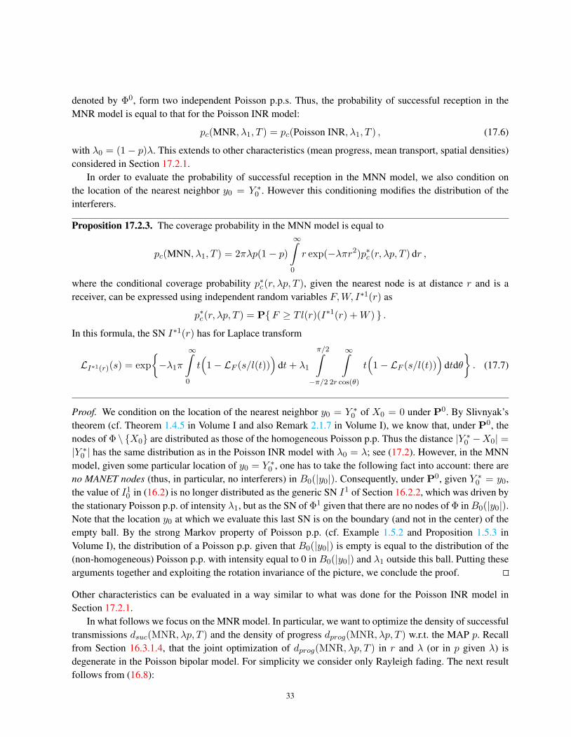
denoted by Φ0, form two independent Poisson p.p.s. Thus, the probability of successful reception in theMNR model is equal to that for the Poisson INR model:

pc(MNR, λ1, T ) = pc(Poisson INR, λ1, T ) , (17.6)

with λ0 = (1− p)λ. This extends to other characteristics (mean progress, mean transport, spatial densities)considered in Section 17.2.1.

In order to evaluate the probability of successful reception in the MNN model, we also condition onthe location of the nearest neighbor y0 = Y ∗0 . However this conditioning modifies the distribution of theinterferers.

Proposition 17.2.3. The coverage probability in the MNN model is equal to

pc(MNN, λ1, T ) = 2πλp(1− p)∞∫

0

r exp(−λπr2)p∗c(r, λp, T ) dr ,

where the conditional coverage probability p∗c(r, λp, T ), given the nearest node is at distance r and is areceiver, can be expressed using independent random variables F,W, I∗1(r) as

p∗c(r, λp, T ) = P{F ≥ T l(r)(I∗1(r) +W ) } .

In this formula, the SN I∗1(r) has for Laplace transform

LI∗1(r)(s) = exp{−λ1π

∞∫0

t(

1− LF (s/l(t)))

dt+ λ1

π/2∫−π/2

∞∫2r cos(θ)

t(

1− LF (s/l(t)))

dtdθ}. (17.7)

Proof. We condition on the location of the nearest neighbor y0 = Y ∗0 of X0 = 0 under P0. By Slivnyak’stheorem (cf. Theorem 1.4.5 in Volume I and also Remark 2.1.7 in Volume I), we know that, under P0, thenodes of Φ \ {X0} are distributed as those of the homogeneous Poisson p.p. Thus the distance |Y ∗0 −X0| =|Y ∗0 | has the same distribution as in the Poisson INR model with λ0 = λ; see (17.2). However, in the MNNmodel, given some particular location of y0 = Y ∗0 , one has to take the following fact into account: there areno MANET nodes (thus, in particular, no interferers) in B0(|y0|). Consequently, under P0, given Y ∗0 = y0,the value of I1

0 in (16.2) is no longer distributed as the generic SN I1 of Section 16.2.2, which was driven bythe stationary Poisson p.p. of intensity λ1, but as the SN of Φ1 given that there are no nodes of Φ inB0(|y0|).Note that the location y0 at which we evaluate this last SN is on the boundary (and not in the center) of theempty ball. By the strong Markov property of Poisson p.p. (cf. Example 1.5.2 and Proposition 1.5.3 inVolume I), the distribution of a Poisson p.p. given that B0(|y0|) is empty is equal to the distribution of the(non-homogeneous) Poisson p.p. with intensity equal to 0 in B0(|y0|) and λ1 outside this ball. Putting thesearguments together and exploiting the rotation invariance of the picture, we conclude the proof.

Other characteristics can be evaluated in a way similar to what was done for the Poisson INR model inSection 17.2.1.

In what follows we focus on the MNR model. In particular, we want to optimize the density of successfultransmissions dsuc(MNR, λp, T ) and the density of progress dprog(MNR, λp, T ) w.r.t. the MAP p. Recallfrom Section 16.3.1.4, that the joint optimization of dprog(MNR, λp, T ) in r and λ (or in p given λ) isdegenerate in the Poisson bipolar model. For simplicity we consider only Rayleigh fading. The next resultfollows from (16.8):

33

Proposition 17.2.4. Consider the MNR model with Rayleigh fading, OPL 3 path loss model and no noise(W = 0). The density of successful transmission and the density of progress in this model are equal to

dsuc(MNR, λp, T ) =λp(1− p)

(1− p) + pT 2/βK(β)/π, (17.8)

dprog(MNR, λp, T ) =

√λp(1− p)

2(

(1− p) + pT 2/βK(β)/π)3/2

. (17.9)

It is easy to see that both densities dsuc and dprog attain their maximal values for some 0 < p < 1that does not depend on λ. For example the density of success admits the following optimal tuning of theparameter p.

Corollary 17.2.5. Under the assumptions of Proposition 17.2.4, we have

arg max0≤p≤1

dsuc(MNR, λp, T ) =1

1 + T 1/β√K(β)/π

,

max0≤p≤1

dsuc(MNR, λp, T ) =λ(

1 + 1

T 1/β√K(β)/π

)(1 + T 1/β

√K(β)/π

) .

17.3 Multicast Mode

In this section we consider the situation where each transmitter broadcasts some common data to manyreceiving nodes (see Chapter 25). More precisely, as in the MNR model considered above, we assume thatthe potential receivers Φ0 = Φ0 = Φ \ Φ1 are those nodes of the MANET Φ which are not authorized totransmit at the considered time slot (a similar analysis can be done for other receiver models) and that eachtransmitter of this time slot targets all the potential receivers of Φ0.

The model features an i.m. p.p. Φ = {Xi, ei,Fi} with Poisson nodes Φ = {Xi} and their MAC indica-tors {ei} as in Section 16.2.1, except that no prescribed receivers {yi} are considered; the virtual powers F jihave the following modified interpretation:

(4’) F ji denotes the virtual power emitted by node i (provided ei = 1) towards node j in Φ0.

17.3.1 SINR-neighbors

Let us consider the coverage scenario of Section 16.2.2 in which a successful transmission requires a SINRnot smaller than some threshold T . More precisely, adapting Definition 16.2.1 to the present scenario, wesay that Xj successfully captures the signal from Xi if

SINRij =F ji /l(|Xi −Xj |)

W + I1ij

≥ T , (17.10)

where I1ij =

∑Xk∈Φ1,k 6=i,j F

jk/l(|Xk −Xj |).

34

Definition 17.3.1. Define the set of SINR-neighbors V (Xi) = V (Xi, Φ) of Xi ∈ Φ as the union of {Xi}and of the subset of potential receivers of Φ0 which successfully capture the packet transmitted by Xi (if Xi

transmits at the given time slot):

V (Xi) = {Xi} ∪

{{Xj : Xj ∈ Φ0 s.t. δ(Xi, Xj) = 1} ifXi ∈ Φ1

∅ otherwise,(17.11)

with δ(Xi, Xj) the indicator of the SINR condition (17.10).

Remark 17.3.2. Nothing guarantees that the receivers of two different transmitters are different, so thatunless a receiver can capture two different packets at the same time, a new type of collision should be takeninto account. However, if T ≥ 1, no two transmitters can ever be successful with the same receiver. Indeed, itfollows from Lemma 17.3.4 that when T ≥ 1 (which is often the case in practice), ifX1 andX2 both belongto Φ1, then V (X1) ∩ V (X2) = ∅. Hence, even in the case where receivers cannot capture two differentpackets at the same time, this type of collision actually never happens for such T .

In what follows we focus on the properties of the set of SINR neighbors of the typical node. For this wedefine the directed graph GSINR with set of nodes Φ and with directed edges connecting each Xi to each ofits neighbors V (Xi) (this graph was already considered in Chapter 8 in Volume I).

The number Houti = card(V (Xi)) of SINR neighbors of node Xi in GSINR is called the out-degree ofthis node. If Xi transmits, the out-degree of Xi is the number of nodes which receive the packet transmittedby node Xi plus 1 (due to the convention that Xi ∈ V (Xi)). If Xi does not transmit, then its out-degree is1. Similarly, the in-degreeHini of Xj ∈ Φ is 1 if this node is a transmitter; if it is not a transmitterHini is thenumber of transmitters captured by Xi at the given time slot, plus 1.

Note that Houti and Hini may be considered as new marks of the nodes of Φ and that the process Φenriched by these mark is still stationary (cf. Definition 2.1.4 in Volume I).

Denote by hout and hin the expected out- and in-degree, respectively, of the typical node of Φ:

hout = E0[Hout0 ], hin = E0[Hin0 ].

Notice that hout (resp. hin) is also the spatial average of the node out-degrees (resp. in-degree) due to thefact that our i.m. Poisson p.p. Φ is ergodic.

The first key result regarding the mean degrees of GSINR follows from the mass transport principle:

Proposition 17.3.3. The mean in-degree of the typical node of GSINR and its mean out-degree are equal; i.e.hin = hout = h.

Proof. This result should not be surprising. Each directed edge has two ends; call them edge-source andedge-destination, respectively. Heuristically (and this argument can be made precise using ergodic theory),hin corresponds to the average number of edge-destinations per node, while hout the average number ofedge-sources per node. Since one edge-source corresponds exactly to one edge-destination both averagesshould coincide.

35

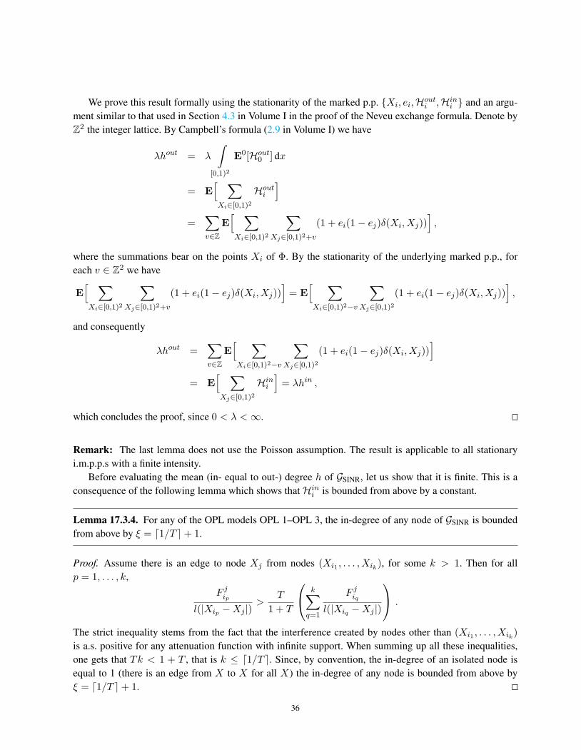
We prove this result formally using the stationarity of the marked p.p. {Xi, ei,Houti ,Hini } and an argu-ment similar to that used in Section 4.3 in Volume I in the proof of the Neveu exchange formula. Denote byZ2 the integer lattice. By Campbell’s formula (2.9 in Volume I) we have

λhout = λ

∫[0,1)2

E0[Hout0 ] dx

= E[ ∑Xi∈[0,1)2

Houti

]=

∑v∈Z

E[ ∑Xi∈[0,1)2

∑Xj∈[0,1)2+v

(1 + ei(1− ej)δ(Xi, Xj))],

where the summations bear on the points Xi of Φ. By the stationarity of the underlying marked p.p., foreach v ∈ Z2 we have

E[ ∑Xi∈[0,1)2

∑Xj∈[0,1)2+v

(1 + ei(1− ej)δ(Xi, Xj))]

= E[ ∑Xi∈[0,1)2−v

∑Xj∈[0,1)2

(1 + ei(1− ej)δ(Xi, Xj))],

and consequently

λhout =∑v∈Z

E[ ∑Xi∈[0,1)2−v

∑Xj∈[0,1)2

(1 + ei(1− ej)δ(Xi, Xj))]

= E[ ∑Xj∈[0,1)2

Hini]

= λhin ,

which concludes the proof, since 0 < λ <∞.

Remark: The last lemma does not use the Poisson assumption. The result is applicable to all stationaryi.m.p.p.s with a finite intensity.

Before evaluating the mean (in- equal to out-) degree h of GSINR, let us show that it is finite. This is aconsequence of the following lemma which shows thatHini is bounded from above by a constant.

Lemma 17.3.4. For any of the OPL models OPL 1–OPL 3, the in-degree of any node of GSINR is boundedfrom above by ξ = d1/T e+ 1.

Proof. Assume there is an edge to node Xj from nodes (Xi1 , . . . , Xik), for some k > 1. Then for allp = 1, . . . , k,

F jipl(|Xip −Xj |)

>T

1 + T

k∑q=1

F jiql(|Xiq −Xj |)

.

The strict inequality stems from the fact that the interference created by nodes other than (Xi1 , . . . , Xik)is a.s. positive for any attenuation function with infinite support. When summing up all these inequalities,one gets that Tk < 1 + T , that is k ≤ d1/T e. Since, by convention, the in-degree of an isolated node isequal to 1 (there is an edge from X to X for all X) the in-degree of any node is bounded from above byξ = d1/T e+ 1.

36

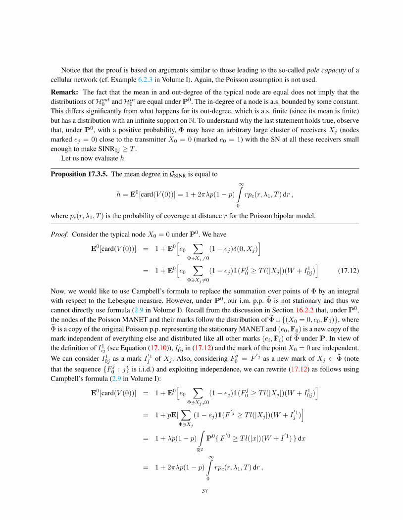
Notice that the proof is based on arguments similar to those leading to the so-called pole capacity of acellular network (cf. Example 6.2.3 in Volume I). Again, the Poisson assumption is not used.

Remark: The fact that the mean in and out-degree of the typical node are equal does not imply that thedistributions ofHout0 andHin0 are equal under P0. The in-degree of a node is a.s. bounded by some constant.This differs significantly from what happens for its out-degree, which is a.s. finite (since its mean is finite)but has a distribution with an infinite support on N. To understand why the last statement holds true, observethat, under P0, with a positive probability, Φ may have an arbitrary large cluster of receivers Xj (nodesmarked ej = 0) close to the transmitter X0 = 0 (marked e0 = 1) with the SN at all these receivers smallenough to make SINR0j ≥ T .

Let us now evaluate h.

Proposition 17.3.5. The mean degree in GSINR is equal to

h = E0[card(V (0))] = 1 + 2πλp(1− p)∞∫

0

rpc(r, λ1, T ) dr ,

where pc(r, λ1, T ) is the probability of coverage at distance r for the Poisson bipolar model.

Proof. Consider the typical node X0 = 0 under P0. We have

E0[card(V (0))] = 1 + E0[e0

∑Φ3Xj 6=0

(1− ej)δ(0, Xj)]

= 1 + E0[e0

∑Φ3Xj 6=0

(1− ej)1(F j0 ≥ T l(|Xj |)(W + I10j)]

(17.12)

Now, we would like to use Campbell’s formula to replace the summation over points of Φ by an integralwith respect to the Lebesgue measure. However, under P0, our i.m. p.p. Φ is not stationary and thus wecannot directly use formula (2.9 in Volume I). Recall from the discussion in Section 16.2.2 that, under P0,the nodes of the Poisson MANET and their marks follow the distribution of Φ∪ {(X0 = 0, e0,F0)}, whereΦ is a copy of the original Poisson p.p. representing the stationary MANET and (e0,F0) is a new copy of themark independent of everything else and distributed like all other marks (ei,Fi) of Φ under P. In view ofthe definition of I1

ij (see Equation (17.10)), I10j in (17.12) and the mark of the pointX0 = 0 are independent.

We can consider I10j as a mark I

′1j of Xj . Also, considering F j0 = F

′j as a new mark of Xj ∈ Φ (notethat the sequence {F j0 : j} is i.i.d.) and exploiting independence, we can rewrite (17.12) as follows usingCampbell’s formula (2.9 in Volume I):

E0[card(V (0))] = 1 + E0[e0

∑Φ3Xj 6=0

(1− ej)1(F j0 ≥ T l(|Xj |)(W + I10j)]

= 1 + pE[∑

Φ3Xj

(1− ej)1(F′j ≥ T l(|Xj |)(W + I

′1j )]

= 1 + λp(1− p)∫R2

P0{F ′0 ≥ T l(|x|)(W + I′1) } dx

= 1 + 2πλp(1− p)∞∫

0

rpc(r, λ1, T ) dr ,

37

where the last equality follows from the fact that F′0, I

′1 have the same distributions as the generic variablesF, I1 considered in Section 16.2.2.

In the case of Rayleigh fading, by Proposition 16.2.2, we obtain the following more explicit result:

Corollary 17.3.6. For Rayleigh fading, the mean degree of the typical node of the graph GSINR is equal to

h = E0[card(V (0))] = 1 + λp(1− p)2π∞∫

0

LW (µT l(r)) exp{−2πλp

∞∫0

v

1 + l(v)/(T l(r))dv}rdr .

In particular, for W ≡ 0 and OPL 3,

h = 1 +(1− p)πT 2/βK(β)

, (17.13)

where K(β) is defined in (16.9).

We consider now the case where F has a general distribution.Recall from Section 16.2.4 that pc(r) = pc(r, 1, 1) denotes the value of the probability of coverage

calculated in the Poisson bipolar MANET model with T ≡ 1, λ1 = 1,W ≡ 0 and normalized virtualpowers distributed as F = µF .

Using Proposition 17.3.5 and the scaling properties of the coverage probability expressed in Proposi-tion 16.2.9, we get:

Corollary 17.3.7. Assume W ≡ 0, OPL 3 and a general distribution of F . The mean degree of the typicalnode of the graph GSINR is equal to

h = 1 +(1− p)2πT 2/β

∞∫0

spc(s) ds , (17.14)

where the constant∫∞

0 spc(s) ds does not depend on any parameter of the model other than the distributionof the normalized virtual power F .

This gives the dependence of the mean degree h in function of the basic model parameters. In particular,we have the same invariance w.r.t. the node density λ as in the coverage probability.

17.3.2 Shannon Multicast Throughput

Consider a multicast scenario with an adaptive coding scheme leading to the Shannon throughput introducedin Section 16.2.3. More precisely, we suppose that each transmitter Xi, ei = 1 broadcasts some informationusing a multi-layer coding scheme that allows each receiver Xj , ej = 0 to receive this information with thethroughput Tij = log(1 + SINRij) (for instance in video broadcast, if the throughput is high, several layersare sent and the video signal is received with high resolution; if it is low, fewer layers are sent and the qualityis lower). Denote by T outi = ei

∑Xj∈Φ0 Tij the total rate with which node Xi floods the network when it

is transmitting. Similarly, denote by T ini = (1 − ei)∑

X∈Φ1 Tji the total rate with which receiver Xi canreceive information from all MANET nodes. Let τ in = E0[T in0 ] and τ out = E0[T out0 ].

The following result is another example of the mass transport principle and can be proved along thesame lines as Proposition 17.3.3.

38

Proposition 17.3.8. For the above multicast MANET model, τ in = τ out = τmcast.

The mean total multicast rate τmcast can be evaluated in terms of the mean Shannon throughput in thecorresponding bipolar model. The following result can be proved along the same lines as Proposition 17.3.5.

Proposition 17.3.9. The mean total throughput of a typical node in the multicast MANET model is equalto

τmcast = 2πλp(1− p)∞∫

0

rτ(r, λ1) dr ,

where τ(r, λ1) is the Shannon throughput evaluated for the Poisson bipolar model.

Using formula (16.13) and Proposition 17.3.5, τmcast can be further related to the coverage probabilitypc(r, λ1, ·) and (interchanging the order of integration) to the mean degree of the multicast graph GSINR. Inparticular, the following result follows from Proposition 17.3.9, formula (16.13) and the scaling propertiesof the coverage probability expressed in Proposition 16.2.9.

Corollary 17.3.10. Assume W ≡ 0, OPL 3 and a general distribution of F . The mean total throughput oftypical node in the multicast MANET model described above is equal to

τmcast = (1− p)βK(β)

∞∫0

spc(s) ds , (17.15)

where K(β) is defined in (16.9) and the constants∫∞

0 spc(s) ds do not depend on any parameter of themodel other than the distribution of the normalized virtual power F . In particular, for Rayleigh fading(exponential F )

τmcast =(1− p)β

2. (17.16)

17.4 Opportunistic Receivers – MAC and Routing Cross-Layer Optimization

In this section we focus on:

• The outage scenario, where a transmission requires a SINR larger than some threshold T ;• The MANET receiver scenario, where the nodes Φ0 = Φ0 = Φ \ Φ1 which are not allowed to

access the shared medium form the set of potential receivers;• The opportunistic routing scenario, where the receiver of a given transmitter is not prescribed in

advance but rather selected so as to maximize the packet progress in a given direction.

17.4.1 Receivers Maximizing Instantaneous Directional Progress

To consider directional progress we need to extend the i.m. p.p. Φ by introducing marks di; the latter arei.i.d. unit vectors in R2 representing directions in which the nodes aim to send their packets. The MANET

39

model considered in this section assumes an i.m. p.p. Φ = {Xi, ei, di,Fi} with Poisson nodes Φ = {Xi}and their MAC indicators {ei} as in Section 16.2.1, with the random cross-fading model with virtual powersFi (see (4’) of Section 17.3). In the opportunistic receiver selection:

(3”) The receiver yi of the transmitter Xi ∈ Φ is its SINR neighbor (cf. Definition 17.3.1) whichmaximizes the effective progress of the transmitted packet in the direction di

yi = arg maxXj∈V (Xi)

{〈Xj −Xi, di〉} . (17.17)

Note that V (Xj) is non-empty (Xi ∈ V (Xi)) and almost surely finite (cf. Lemma 17.3.4). Then the“arg max” in the definition of yi is almost surely well defined for all i (cf. also Lemma 4.2.2 in Volume I).

A major difference between this opportunistic mechanism and all previously considered cases is that ithas much more chance to lead to a successful transmission: for instance, assume that the direction d0 of nodeX0 = 0 (under P0) is that of the x axis; then as soon as X0 has SINR neighbors with a positive abscissa,the transmission is successful. Note that since Xi ∈ V (Xi) the maximal value of 〈Xj −Xi, di〉 in (17.17)is at least 0 and the case when the arg max is attained on Xi is considered as an unsuccessful transmission.

Denote by Di the effective directional progress of the packet transmitted in the given time slot by trans-mitter Xi:

Di = 〈yi −Xi, di〉 = maxXj∈Φ0

{〈Xj −Xi, di〉+δ(Xi, Xj)} , (17.18)

where a+ = a1(a > 0).In what follows we focus on the mean effective directional progress of the packet transmitted by the

typical node of the MANET given it is transmitting in the tagged time slot:

prog(λ, p) = E0[D0 | e0 = 1]

and on the spatial density of this progress:

dprog(λ, p) = λp prog(λ, p) = λE0[D0] ,

where the notation is meant to stress the difference with the effective progress (16.19) and its density (16.22)as considered in the bipolar network model.

17.4.2 Optimization of the Spatial Density of Directional Progress

One of the main objects of this subsection is

p∗ = arg max0<p≤1

{dprog(λ, p)} , (17.19)

whenever the argmax is well defined.In § 16.3.1.4 we saw that in the Poisson bipolar MANET model, the joint optimization of the density of

progress dprog(r, λ1, T ) in p and in the transmission distance r led to degenerate answers due to the fact thatin this model r is not related to the node density.

In contrast, the next lemma shows that the optimization of dprog(λ, p) w.r.t. p is not degenerate (i.e.p = 0 is not the optimal solution). For simplicity we limit ourselves to the OPL 3 model and to Rayleighfading. This result can be extended to more general situations under some conditions on the moments of Fand/or W .

40

Lemma 17.4.1. Assume the OPL 3 model and Rayleigh fading. Then limp→0 dprog(λ, p) = 0 anddprog(λ, 1) = 0.

Proof. Note that D0 increases when the thermal noise decreases. Thus it is enough to prove the result forW = 0, which we assume in what follows. We have

E0[D0 | e0 = 1] =

∞∫0

P0{D0 > s | e0 = 1 } ds

=

∞∫0

P0{V (0) ∩Bc0(s) 6= ∅ | e0 = 1 } ds

≤∞∫

0

min{

1,E0[card(V (0) ∩Bc0(s)) | e0 = 1]

}ds . (17.20)

Following the same arguments as those used to express E0[card(V (0))] in the proof of Proposition 17.3.5and (16.8), we have

E0[card(V (0) ∩Bc0(s)) | e0 = 1] = 2πλ(1− p)

∞∫s

rpc(r, λ1, T ) dr

= 2πλ(1− p)∞∫s

r exp(−λpr2T 2/βK(β)) dr

=π(1− p)pT 2/βK(β)

exp(−λps2T 2/βK(β)) .

The last expression is smaller than 1 for

s ≥ s0(p) =

√1

λpT 2/βK(β)

(log( π(1− p)pT 2/βK(β)

))+

.

Using (17.20), we obtain

λpE0[D0 | e0 = 1] ≤ λps0(p) +πλ(1− p)T 2/βK(β)

∞∫s0(p)

exp(−λps2T 2/βK(β)) ds

= λps0(p) +π√λ(1− p)

√pT 3/βK(β)3/2

∞∫s0(p)√λpT 2/βK(β)

e−s2

ds . (17.21)

Note that s0(1) = 0 and∫∞

0 e−s2

ds < ∞; thus expression (17.21) is equal to 0 for p = 1. In order toevaluate the limit of this expression when p → 0, we use the inequality

∫∞x e−s

2ds ≤ e−x

2, which holds

true for all x ≥ 1/2 (to prove this, one can use the fact that e−s2 ≤ e−x

2+x−s for s ≥ x ≥ 1/2). Note that

41

√ps0(p) ∼

√log(1/p)→∞ when p→ 0. Thus using (17.21) for sufficiently small p, we have

λpE0[D0 | e0 = 1] ≤ λps0(p) +π√λ(1− p)

√pT 3/βK(β)3/2

exp(−s2

0(p)λpT 2/βK(β))

= λps0(p) +√λp

T 1/βK(β)1/2

which tends to 0 when p→ 0 since ps0(p) ∼√p log(1/p)→ 0. This completes the proof.

The following invariance of p∗ with respect to λ can be proved using some refinements of the argumentsused in the proof of Proposition 16.2.9.

Proposition 17.4.2. Assume W = 0, OPL 3 and a general distribution for F . Then the maximal density ofdirectional progress dprog(λ, p) is attained for the MAP p∗ = p∗(T ) satisfying√

p∗H(p∗, T ) = sup0≤p≤1

√pH(p, T ),

for some function H(p, T ) that does not depend on λ.

Remark: This proposition has an important practical implication: it implies that the parameter p can beoptimally tuned regardless of the spatial density of network nodes.

Proof. (of Proposition 17.4.2) The nodes of the Poisson p.p. Φ = {Xi} with intensity λ can be representedas {Xi = X ′i/

√λ }, where Φ′ = {X ′i} is a Poisson with intensity 1 (cf. Example 1.3.12 in Volume I). Let

Φ′ and Φ be the respective marked versions of these p.p.s with (path-wise) the same marks (i.e. the mark ofeach X ′i is equal to that of Xi). Note that under our OPL 3 and W = 0 assumptions, the SINR (in fact theSIR) is invariant with respect to dilations of the points of the p.p. Indeed,

l(|X ′i/√λ−X ′j/

√λ|) = λβ/2l(|X ′i −X ′j |)

and the factor λβ/2 cancels out in the numerator and the denominator of the SINR expression in caseW = 0.This means that

V (Xi, Φ) = 1/√λV (X ′i, Φ

′).

Moreover, the dilation (our scaling) is a conformal mapping (preserves angles). Consequently, the receiver yichosen in V (Xi) according to the maximal directional progress principle (17.17) is equal to y′i/

√λ, where

y′i is chosen in V (X ′i, Φ′) according to the same principle. This concludes the proof.

The functions dprog(λ, p) and H(p, T ) are not known in closed form. In the next section we derive somebounds for them.

17.4.3 *Modified Progress — Bounds on Mean Progress

Consider the following function of Φ under P0, that we call modified progress.

D0 = maxXj∈Φ0

{〈Xj , d0〉+pc(|Xj |, λp, T )} . (17.22)

42

The only difference between progress D0 and modified progress D0 is that one replaces the (random)indicator δ(0, Xj) by the expectation of this indicator given Xj , namely pc(|Xj |, λ1, T ) in the max.This modification will allow us to evaluate the mean values of prog(λ, p) = E0[D0 | e0 = 1] anddgprog(λ, p) = λp prog(λ, p). It is also of practical interest as the latter gives a lower bound to the for-mer:

Proposition 17.4.3. For all λ, p we have prog(λ, p) ≥ prog(λ, p). In consequence dprog(λ, p) ≥dgprog(λ, p).

Proof. Recall that by the property of the independent thinning of Poisson p.p. (cf. Proposition 1.3.5 inVolume I), Φ1 and Φ0 form two independent Poisson p.p’s. Since under P0, givenXj , the indicator δ(0, Xj)is a functional of Φ1 we have

E[D | e0 = 1] = E0[

maxXj∈Φ0

{〈Xj , di〉+pc(|Xj |, λp, T )

} ∣∣∣ e0 = 1]

= E0[

maxXj∈Φ0

{〈Xj , di〉+E0[δ(0, Xj) |Φ0]

} ∣∣∣ e0 = 1]

= E0[

maxXj∈Φ0

{E0[〈Xj , di〉+δ(0, Xj) |Φ0]

} ∣∣∣ e0 = 1]

≤ E0[E0[

maxXj∈Φ0

{〈Xj , di〉+δ(0, Xj)

} ∣∣∣Φ0] ∣∣∣ e0 = 1

]= E0[D0 | e0 = 1] ,

where the last but one step follows from the following simple fact: for any r.vs Z1, Z2, . . . we havemaxi{E[Zi]} ≤ maxi{E[maxi{Zi}]}.

We now focus on the evaluation of prog(λ, p). For this, we use the notation introduced in Sec-tion 16.3.1.3, and in particular: rmax = rmax(λp) = arg maxr≥0{prog(r, λp, T )} and ρ = ρ(λp) =prog(rmax(λ, p), λp, T )}.

For z ∈ [0, 1], let

G(z) =2r2

max

∫{r≥0:ρz/(rpc(r))<1}

r arccos( ρz

rpc(r)

)dr , (17.23)

where the arguments pλ and T are omitted.

Remark 17.4.4. For the GI0+M/GI model with OPL 3, Proposition 16.3.7 shows that G(z) does not depend on

the model parameters λ, p, T, µ. Indeed, in this case

G(z) =2

const3

∫{r≥0:const4z/(rpc(r))<1}

r arccos(

const4zrpc(r)

)dr ,

with pc(·) the function defined in Lemma 16.2.9. In particular, for Rayleigh fading, we have

G(z) = 2∫

{t:et/√

2et≤1/z}

arccos( zet√

2et

)dt . (17.24)

The main result concerning D is:

43

Proposition 17.4.5. We have

FD(z) = P0{ D ≤ z | e0 = 1 } = e−λ(1−p)(rmax(λp))2G(z/ρ(λp)) (17.25)

and

prog(λ, p) = E0[D | e0 = 1] = ρ(λp)

1∫0

1− e−λ(1−p)(rmax(λp))2G(z) dz . (17.26)

Proof. Note in (17.22) that under P0 given e0 = 1 and d0 the variable D has the form of an extremal SNmaxXi∈Φ0 g(Xi) with the response function g(x) = pc(|x|)〈x, d0〉+.

Using Proposition 2.4.2 in Volume I, we get:

P(D ≤ z) = exp[−λ(1− p)

∫R2

1(g(x) > z) dx].

Passing to polar coordinates, we get∫R2

1(g(x) > z) dx = r2maxG(z/ρ) ,

which completes the proof.

Corollary 17.4.6. For the GI0+M/GI model with OPL 3,

prog(λ, p) =const4

T 1/β√λpH(p, T ) (17.27)

dgprog(λ, p) =const4

√λp

T 1/βH(p, T ) , (17.28)

where

H(p, T ) =

1∫0

1− exp[(

1− 1p

) G(z)const3T 2/β

]dz . (17.29)

Note that we have the same scaling of dgprog(λ, p) in the main parameters of the model as that of dprog(λ, p)given in Proposition 17.4.2.

Corollary 17.4.7. Under the assumptions of Corollary 17.4.6, the maximal density of modified progressdgprog(λ, p) is attained for the MAP p∗ = p∗(T ) satisfying√

p∗H(p∗, T ) = sup0≤p≤1

√pH(p, T ).

If such p∗ exists, it does not depend on λ. For Rayleigh fading, this is equivalent to1∫

0

(1 +

G(z)p∗T 2/βC

)exp[(

1− 1p∗

) G(z)2T 2/βC

]dz = 1 . (17.30)

44

G(z)

0

10

20

30

40

50

60

0 0.2 0.4 0.6 0.8 1

z

dprog(λ, p)

0.002

0.003

0.004

0.005

0.006

0.007

0.008

0.009

0 0.02 0.04 0.06 0.08 0.1 0.12 0.14 0.16

10dB

13dB

15dB

p

Fig. 17.1 Left: Plot of the function G∼ with points representing values of G. The total relative error 136

rP (G(z)−G∼(z))2

G2(z), where the

summation is taken over 36 points marked on the plot, is less then 1.27%. Right: Density of modified progress dprog(λ, p) for the M0+M/M

model with OPL 3. Here β = 3, λ = 1 and with T = {10, 13, 15}dB (curves from top to bottom). The optimal values (arg max,max) are{(0.052, 0.0086), (0.035, 0.0055), (0.026, 0.0040)} respectively.

Example 17.4.8. The aim of the present example is to numerically evaluate the G function defined in(17.23) and efficiently trace the function dgprog(λ, p) in the M

0+M/M model with OPL 3. For this, we usethe so-called Lambert W functions LW0 and LW1. These functions can be seen as inverse of the functiont → tet in the domains (−1,∞) and (−∞,−1) respectively; more precisely, for s ≥ −1/e, LW0(s) is theunique solution of LW0(s)eLW0

(s) = s satisfying LW0(s) ≥ −1, whereas for 0 > s ≥ −1/e, LW1(s) isthe unique solution of LW1(s)eLW1

(s) = s satisfying LW1(s) ≤ −1. Let L0(s) = −12LW0(−s−2e−1) and

L1(s) = −12LW1(−s−2e−1) . The following representation of G is equivalent to that in (17.24):

G(z) = 2

L1(1/z)∫L0(1/z)

(L1(s)− L0(s)

)ds ,

= 2

π/2∫arcsin(z)

(L1

(sin sz

)− L0

(sin sz

))ds .

Moreover, the following function

G∼(z) = π(1− z)− 2 ln(z) arccos(z)

approximates G very well over the whole interval 0 < z < 1; cf. Figure 17.1 (Left). We use this approxi-mation to calculate numerically the value of dgprog(λ, p). Figure 17.1 (Right) shows the results for β = 3,λ = 1 and three values of the SINR threshold T = {10, 13, 15}dB. On the plot, we can identify the MAPp∗ that maximizes the density of progress for a given T .

45

17.4.4 *Location of the Optimal Receiver

17.4.4.1 Comparison to the Case with a Restricted Range for Receivers

In what follows we show that each transmitter can restrict its search for an optimal receiver to its vicinity.For this we show first that the optimal density of progress can be approximated by that in a model wherethe domain of reception is restricted to a certain neighborhood of the transmitter. By this we mean that weexclude in the definition of D or D the receivers lying outside some disk with a given radius R.

We have the following straightforward generalization of our previous results:

Proposition 17.4.9. Propositions 17.4.3 and 17.4.5 remain true if we take maxXi∈Φ0,|Xj |≤R(. . .) (withmax ∅ = 0) in (17.18) and (17.22). In this case the function G has to be modified by taking the integralin (17.23) over the region {0 ≤ r ≤ R : ρz/(rpc(r)) < 1}.

The case considered above will be referred to as the restricted range model in what follows.We look for a reception radius R such that for a given p, the density of progress in the restricted range

model is close enough to that of the unrestricted range model. It is convenient to relate the reception radiusR to the intensity λ of transmitters. As we shall see later on, it is convenient to take R = Krmax forsome constant K ≥ 0 (recall, that rmax = rmax(λp) is the distance at which the progress prog(r, λp, T ) =rpc(r, λp, T ) in the corresponding bipolar model is maximal). Denote byGK the function defined by (17.23)with the integral taken over {0 ≤ r ≤ Krmax : ρz/(rpc(r)) < 1} and by progK = progK(λ, p) theassociated mean modified progress in the restricted range model.

We have the following continuity result regarding progK and prog = prog(λ, p).

Proposition 17.4.10. For the GI0+M/GI model with OPL 3 and P{F > 0 } > 0.

0 ≤ prog − progK ≤ ρzK , (17.31)

for some function K 7→ zK , such that limK→∞ zK = 0. For Rayleigh fading, we can take zK =Ke1/2−K2/2, for K ≥ 1.

Proof. Let pc(·) be the function defined in Lemma 16.2.9. By Proposition 17.3.5 and Lemma 17.3.4 weknow that

∫∞0 rpc(r) dr < ∞. Moreover, by Proposition 16.3.6 and Proposition 2.2.6 in Volume I we

know that pc(r) is continuous in r. Thus, rpc(r) → 0 when r → ∞ and for any K ≥ 0, there exists zKsuch that GK(z) = G(z) for z ≥ zK . Moreover zK → 0 when K → ∞. Thus (17.31) follows fromPropositions 17.4.5 and 17.4.9.

Example 17.4.11. Take for example, p = 0.035, T = 13dB and Rayleigh fading. In this case, the meanmodified progress in the unrestricted model is approximately prog = 0.0055/0.035 = 0.157 (cf. Figure 17.1Right), whereas the best mean range is attained for the range attempt rmax = 0.506 and is equal to ρ = 0.307.In order to have a relative difference ε = 0.01 we find the minimal K ≥ 1 such that Ke1/2−K2/2 ≤0.01 · 0.157/0.307 = 0.00513, which is K = 3.768. This means that in the model with reception radiusR = Krmax = 3.768 · 0.506 = 1.905, the mean modified progress (and its spatial density) is within 1% ofthe optimal value of the mean modified progress obtained in the unrestricted model.

46

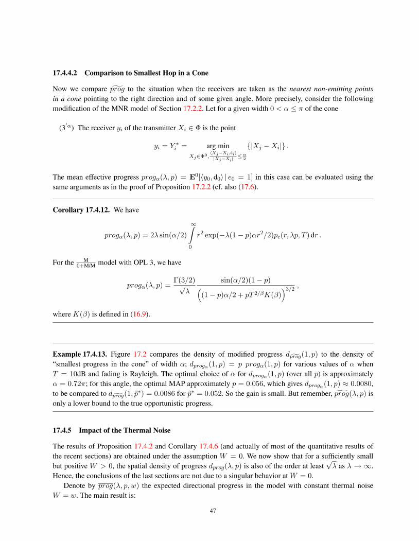
17.4.4.2 Comparison to Smallest Hop in a Cone

Now we compare prog to the situation when the receivers are taken as the nearest non-emitting pointsin a cone pointing to the right direction and of some given angle. More precisely, consider the followingmodification of the MNR model of Section 17.2.2. Let for a given width 0 < α ≤ π of the cone

(3′α) The receiver yi of the transmitter Xi ∈ Φ is the point

yi = Y ∗i = arg minXj∈Φ0,

〈Xj−Xi,di〉|Xj−Xi|

≤α2

{|Xj −Xi|} .

The mean effective progress progα(λ, p) = E0[〈y0, d0〉 | e0 = 1] in this case can be evaluated using thesame arguments as in the proof of Proposition 17.2.2 (cf. also (17.6).

Corollary 17.4.12. We have

progα(λ, p) = 2λ sin(α/2)

∞∫0

r2 exp(−λ(1− p)αr2/2)pc(r, λp, T ) dr .

For the M0+M/M model with OPL 3, we have

progα(λ, p) =Γ(3/2)√

λ

sin(α/2)(1− p)((1− p)α/2 + pT 2/βK(β)

)3/2,

where K(β) is defined in (16.9).

Example 17.4.13. Figure 17.2 compares the density of modified progress dgprog(1, p) to the density of“smallest progress in the cone” of width α; dprogα(1, p) = p progα(1, p) for various values of α whenT = 10dB and fading is Rayleigh. The optimal choice of α for dprogα(1, p) (over all p) is approximatelyα = 0.72π; for this angle, the optimal MAP approximately p = 0.056, which gives dprogα(1, p) ≈ 0.0080,to be compared to dgprog(1, p∗) = 0.0086 for p∗ = 0.052. So the gain is small. But remember, prog(λ, p) isonly a lower bound to the true opportunistic progress.

17.4.5 Impact of the Thermal Noise

The results of Proposition 17.4.2 and Corollary 17.4.6 (and actually of most of the quantitative results ofthe recent sections) are obtained under the assumption W = 0. We now show that for a sufficiently smallbut positive W > 0, the spatial density of progress dprog(λ, p) is also of the order at least

√λ as λ → ∞.

Hence, the conclusions of the last sections are not due to a singular behavior at W = 0.Denote by prog(λ, p, w) the expected directional progress in the model with constant thermal noise

W = w. The main result is:

47

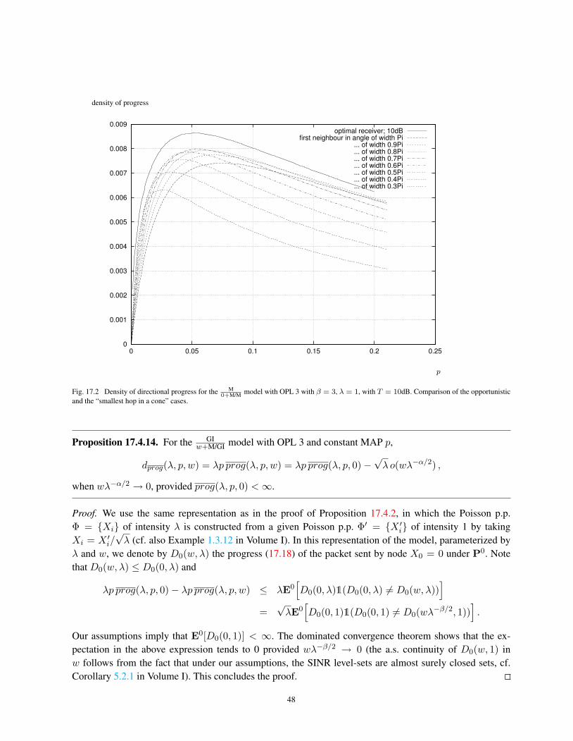
density of progress

0

0.001

0.002

0.003

0.004

0.005

0.006

0.007

0.008

0.009

0 0.05 0.1 0.15 0.2 0.25

optimal receiver; 10dBfirst neighbour in angle of width Pi

... of width 0.9Pi

... of width 0.8Pi

... of width 0.7Pi

... of width 0.6Pi

... of width 0.5Pi

... of width 0.4Pi

... of width 0.3Pi

p

Fig. 17.2 Density of directional progress for the M0+M/M model with OPL 3 with β = 3, λ = 1, with T = 10dB. Comparison of the opportunistic

and the “smallest hop in a cone” cases.

Proposition 17.4.14. For the GIw+M/GI model with OPL 3 and constant MAP p,

dprog(λ, p, w) = λp prog(λ, p, w) = λp prog(λ, p, 0)−√λ o(wλ−α/2) ,

when wλ−α/2 → 0, provided prog(λ, p, 0) <∞.

Proof. We use the same representation as in the proof of Proposition 17.4.2, in which the Poisson p.p.Φ = {Xi} of intensity λ is constructed from a given Poisson p.p. Φ′ = {X ′i} of intensity 1 by takingXi = X ′i/

√λ (cf. also Example 1.3.12 in Volume I). In this representation of the model, parameterized by

λ and w, we denote by D0(w, λ) the progress (17.18) of the packet sent by node X0 = 0 under P0. Notethat D0(w, λ) ≤ D0(0, λ) and

λp prog(λ, p, 0)− λp prog(λ, p, w) ≤ λE0[D0(0, λ)1(D0(0, λ) 6= D0(w, λ))

]=√λE0

[D0(0, 1)1(D0(0, 1) 6= D0(wλ−β/2, 1))

].

Our assumptions imply that E0[D0(0, 1)] < ∞. The dominated convergence theorem shows that the ex-pectation in the above expression tends to 0 provided wλ−β/2 → 0 (the a.s. continuity of D0(w, 1) inw follows from the fact that under our assumptions, the SINR level-sets are almost surely closed sets, cf.Corollary 5.2.1 in Volume I). This concludes the proof.

48

17.5 Local Delays

This section focuses on the packet model. Its main aim is to discuss the mean time to transmit a packetunder Aloha, which will be referred to as the local delay in what follows. This requires the discussion of theunderlying time–space structure. It turns out that this mean time very much depends on the receiver modelwhich is chosen and on the variability of the fading and noise over time.

17.5.1 Space-Time Scenarios

In what follows we add a time-dimension to the basic Poisson bipolar model of Section 16.2.1 and to itsextensions considered in the present chapter, such as the independent Poisson receiver (INR) model, theMANET nearest receiver (MNR) and the nearest neighbor (MNN) model, as well as the multicast model.The idea, already described in Section 2.3.4 in Volume I, consists in assuming that the nodes of the MANETΦ = {Xi} remain unchanged over time and that the marks of these nodes representing their MAC status andother characteristics vary over time. More precisely, consider a common sequence of time slots n = 0, 1, . . .(w.r.t. which all the nodes are perfectly synchronized) and consider the following extensions of the marksintroduced in Section 16.2:

(2s×t) ei(n) is the MAC decision of pointXi of Φ at time n; we always assume that the random variablesei(n) are i.i.d. in i and n; i.e. in space and time, with P{ ei(n) = 1 } = 1−P{ ei(n) = 0 } = p.

(3s×t) yi(n) is the intended receiver of the node i at time n; this receiver may vary over time or notdepending on the receiver model. For example it is fixed (yi(n) ≡ yi) in the basic Poissonbipolar model as well as in the MNN model (cf. (3’) with Φ0 = Φ). On the other hand, it variesin all the models where the choice of the receiver depends on the current MAC status, like forinstance in the MNR and multicast models. For the Poisson INR model one may consider both afixed Poisson receiver p.p. Φ0(n) = Φ0 or a sequence of Poisson p.p.s Φ0(n) which is i.i.d. in n(this might be seen as what happens in the case of receiver Poisson p.p. with high mobility – see1.3.10 in Volume I).

(4s×t) F ji (n) is the virtual power (comprising fading effects) emitted by node i to the receiver of nodej (or to node j in the MANET receiver model) at time n. We adopt the following terminologywith respect to the variability of the virtual powers in time.

– By the fast fading case we understand the scenario when F ji (n) are i.i.d. in n (recall, thatthe default option is that they are also i.i.d. in i, j).

– The slow fading case is that where F ji (n) ≡ F ji , for all n.

Remark: [Terminology] Let us stress that the terminology used here about fading is proper to this mono-graph, where the meaning is that fading remains constant over a slot duration and can be seen as i.i.d. overdifferent time slots. This does not correspond to what is used in many papers of literature. In these papers,fast fading is something not considered here where the channel conditions fluctuate much over a given timeslot. What we call slow fading here would be called shadowing in this literature and what we call fast fadinghere would be be referred to as slow fading.

Regarding the noise variableW , one can consider both i.i.d.W (n) (fast noise) and constantW (n) ≡W(slow noise) scenarios.

49

Note that the p.p. of transmitters Φ1(n) =∑

i δXi1(ei(n) = 1) varies over time due to the MACdecisions. So does the SN

I1i (n) =

∑Xj∈eΦ1(n), j 6=i

F ij (n)/l(|Xj − yi(n)|)

of Φ1(n) \ {Xi} representing the interference at the receiver of the node Xi.Denote by δi(n) the indicator that (16.2) holds at time n (with F , I and W considered at time n);

namely, that location yi(n) (prescribed by the appropriate receiver model) is covered by transmitter Xi withthe required quality at time n.

17.5.2 Local Delay

We now give a general definition of the local delay of the typical node, valid in all our receiver modelsexcept the multicast model of Section 17.3.

Definition 17.5.1. In all single-receiver models, the local delay of the typical node is the number of timeslots needed for node X0 = 0 (considered under the Palm probability P0 with respect to Φ) to successfullytransmit:

L = L0 = inf{n ≥ 1 : δ0(n) = 1} .

This random variable depends on the origin of time (here 1) but we focus on its law below, which does notdepend on the chosen time origin.

The main objective of the remaining part of this section is to study the mean local delay E0[L]. Inparticular, we show that it can be finite or infinite depending on the receiver model and fast or slow fadingand noise model. For some models, it can exhibit the following phase transition: E0[L] <∞ or E0[L] =∞depending on the model parameters (as p, distance r to the receiver, or the mean fading 1/µ). This will bereferred to as the wireless contention phase transition in what follows.

Let S denote all the static elements of the network model: i.e. the elements which are random but whichdo not vary with time n. In all models, we have Φ ∈ S. Moreover, in the slow fading model, we have{Fi} ∈ S and similarly in the slow noise model, W ∈ S . For the fixed Poisson INR and MNN models, wealso have Φ0 ∈ S.

Given a realization of all the elements of S, denote by

πc(S) = E0[e0(1)δ0(1) | S] (17.32)

the conditional probability, given S, that X0 is authorized to transmit by the MAC and that this transmissionis successful at time n = 1. Note that due to our time-homogeneity, this conditional probability does notdepend on n. The following result allows us to express E0[L].

Lemma 17.5.2. In all the receiver models considered above, assuming that the elements which are not static(i.e. which are not in S) are i.i.d., we have

E0[L | S] =1

πc(S)and E0[L] = E0

[ 1πc(S)

]. (17.33)

50

Remark: One can interpret πc(S) as the conditional throughput of node X0, given all the static elementsof the network. Its inverse 1/πc(S) is the conditional local delay of node X0 in this environment. In manycases, this conditional throughput is a.s. positive (so that delays are a.s. finite) for all static environments. Ifthis last condition holds true, by Campbell’s formula, almost surely, all the nodes have a positive conditionalthroughput and finite conditional delay. However, the spatial irregularities of the network imply that thisconditional throughput varies from node to node; in a Poisson configuration, one can find nodes which havean arbitrarily small conditional throughput (and consequently an arbitrarily large conditional delay). Themean local delay E0[L] is the spatial average of these conditional local delays. A finite mean indicates thatthe fraction of nodes in bad shape (for throughput or delay) is in some sense not significant. In contrast,E0[L] = ∞ indicates that an important fraction of the nodes are in a bad shape. This is why the finitenessof the mean local delay is an important performance indicator of the network.

Proof. (of Lemma 17.5.2) Since the elements which are not in S do not change over time, given a realizationof the elements of S, the successive attempts of node X0 to access to the channel and successfully transmitat time n ≥ 1 are independent (Bernoulli) trials with probability of success πc(S). The conditional localdelay L = L0 is then a geometric random variable (the number of trials until the first success in the sequenceof Bernoulli trials) with parameter πc(S). Its (conditional) expectation (given S) is known to be

E0[L | S] =∑n≥1

P0{L ≥ n | S } =∑n≥1

(1− πc(S))n−1 =1

πc(S).

The result follows by integration with respect to the distribution of S .

Example 17.5.3. In order to understand the reasons for which E0[L] may or may not be finite, consider firstthe following two extremal situations. Suppose first that the whole network is independently re-sampledat each time slot (including node locations Φ, which is not our default option). Then S is empty (the σ-algebra generated by it is trivial) and the conditional throughput coincides with the the spatial average ofthe probability of success, namely πc(S) = E0[e0(1)δ0(1)] = p pc, where pc is the coverage probabilityconsidered for the static model. Consequently, in this case of extreme variability (w.r.t. time), we haveE0[L] = 1/(p pc) <∞ provided pc > 0, which holds true under very mild assumptions.

On the other hand, if nothing varies over time (including MAC status, which again is ruled out in ourgeneral assumptions), we have πc(S) = e0(1)δ0(1) (because the conditioning on S determines e0(1)δ0(1)in this case). In this case, under very mild assumptions (e.g. if p < 1), the conditional throughput e0(1)δ0(1)is zero with positive probability, making E0[L] =∞. Note that in this last case, some nodes in the MANETsucceed in transmitting packets every time slot, whereas others never succeed. Having seen the above twoextremal cases, it is not difficult to understand that the mean local delay strongly depends on how much thetime-variability “averages out” the spatial irregularities seen by the MANET nodes.

Note that by Jensen’s inequality,

E0[L] ≥ 1E0[πc(S)]

=1p pc

.

The inequality is in general strict and we may have E0[L] =∞ while pc > 0.In the remaining part of this section we study several particular instances of space-time scenarios.

51

17.5.3 Local Delays in Poisson Bipolar Models

In the Poisson bipolar model, we assume a static location for the MANET nodes Φ and for their receivers{yi}. The MAC variables ei(n) are i.i.d. in i and n. All other elements (fading and noise) follow differenttime scenarios.

17.5.3.1 Slow Fading and Noise Case

Let us consider first the situation where {Fi} and W are static.

Proposition 17.5.4. Assume the Poisson bipolar network model with slow fading and slow noise. If thedistribution of F,W is such that P{WTl(r) > F } > 0, then E0[L] =∞.

Proof. We have

πc(S) = pE0[e0(1)δ0(1) | S]

= pP0{F 00 ≥ T l(r)(W + I1

0 (0)) | S}≤ p1(F 0

0 ≥ T l(r)W ) .

This last indicator is equal to 0 with non-null probability by assumption. Using (17.33), we conclude thatE0[L] =∞.

17.5.3.2 Fast Fading Case

The following auxiliary result will be useful when studying fast Rayleigh fading.

Lemma 17.5.5. Consider the Poisson SN I =∑

Xi∈ΦGi/l(|Xi|), where Φ is some homogeneous Poissonp.p. with intensity α on R2, Gi are i.i.d. random variables with Laplace transform LG(ξ) and l(r) is any re-sponse function (in our case it will always be one of the OPL functions). Denote by LI(ξ |Φ) = E[e−ξI |Φ]the conditional Laplace transform of I given Φ. Then

E[ 1LI(ξ |Φ)

]= exp

{−2πα

∞∫0

v(

1− 1LG(ξ/l(v))

)dv}.

Proof. By the independence of Gi given Φ, we have

E[e−ξI |Φ] =∏Xi∈Φ

E[e−ξLG(ξ/l(|Xi|))]

=∏Xi∈Φ

LG(ξ/l(|Xi|))

= exp{∑Xi∈Φ

log(LG(ξ/l(|Xi|)))}.

Taking the inverse of the last expression and using the known formula for the Laplace transform of thePoisson p.p. (cf. Proposition 1.2.2 in Volume I), we obtain

E[ 1LI(ξ |Φ)

]= exp

{−α

∫R2

(1− e− log(LG(ξ/l(|x|)))

)dx}. (17.34)

52

Passing to polar coordinates completes the proof.

Remark: The extension of the above result to a non-homogeneous Poisson p.p. Φ is straightforward andconsists in replacing the integral α

∫R2(. . .) dx with respect to the Lebesgue measure α dx on R2 in (17.34),

by the integral of the same function with respect to the intensity measure of the considered non-homogeneousPoisson p.p. This extension is useful when we consider the local delay in the MNN model in Section 17.5.4,where the conditioning on the distance to the receiver modifies the intensity of the process of interferers (cf.Proposition 17.2.3) or in the MNN model with closest receiver in a cone (see Remark 17.5.14 below).

Coming back to local delays, let us now consider the situation where the random variables {Fi(n)} arei.i.d. in n. We consider only the Rayleigh fading case.

Proposition 17.5.6. Assume the Poisson bipolar network model with fast Rayleigh fading. We have

E0[L] =1pDW (T l(r)) exp

{2πpλ

∞∫0

vT l(r)l(v) + (1− p)T l(r)

dv},

where

• DW (s) = DslowW (s) = LW (−s) for the slow noise case,• DW (s) = DfastW (s) = 1/LW (s) for the fast noise case.

Proof. In the fast Rayleigh fading case, we have πc(S) = P{F ≥ T l(r)(W + I1) |Φ} for the fast noisecase and πc(S) = P{F ≥ T l(r)(W + I1) |Φ,W} for the slow noise model. Using the assumption on F ,we obtain

πc(S) = LW (µT l(r))E[e−µT l(r)I1 |Φ]

in the fast noise case, andπc(S) = e−µWTl(r)E[e−µT l(r)I

1 |Φ]

for the slow noise case. The result then follows from (17.33) and Lemma 17.5.5 with G = eF . Note that inthis case, LG(ξ) = 1− p+ pLF (ξ), which gives LeF (ξ) = 1− p+ pµ/(µ+ ξ).

Remark 17.5.7 (Wireless contention phase transition for the mean local delay). Proposition 17.5.6shows that in the fast fading and noise case, E0[L] <∞; indeed,

∫∞0 v/l(v) dv <∞. However for the fast

fading and slow noise case, the finiteness of the local delay depends on whether W has finite exponentialmoments of order T l(r)µ. This is a rather strong assumption concerning the tail distribution functionof W . Often this moment is finite only for some sufficiently small value of T l(r)µ. For example, let usassume exponential noise with mean 1/ν. Then LW (−ξ) = ν/(ν − ξ) < ∞ provided T l(r)µ < ν andinfinite for T l(r)µ > ν. This means that in the corresponding Poisson bipolar MANET with a Rayleighfading, exponential noise, we have the following phase transition: the mean local delay is finite wheneverT l(r) < ν/µ and infinite otherwise. Here are a few incarnations of this phase transition:

• For fixed mean transmission power µ−1 (we recall that a typical situation is that where fading hasmean 1 and where µ−1 is actually the effective transmission power) and mean thermal noise ν−1,there is a threshold on the distance r between transmitter and receiver below which the meanlocal delays are finite and above which they are infinite;

53

• For fixed mean thermal noise ν−1 and fixed distance r, there is a threshold on mean transmissionpower µ−1 above which the mean local delays are finite and below which they are infinite;• For fixed mean transmission power µ−1 and fixed distance r, there is a threshold on mean thermal

noise power ν−1 below which the mean local delays are finite and above which they are infinite.

The fact that all transmissions contend for the shared wireless channel may lead to infinite mean local delaysif the system is stressed by either of the phenomena listed above: too distant links, too high a thermal noiseor too low a transmission power.

Remark 17.5.8 (Restart). There is a direct interpretation of the local delay in terms of the so-called Restartalgorithm: assume a file of random size B is to be transmitted over an error prone channel. Let {An}n≥1

be the sequence of channel inter-failure times. If A1 > B (resp. A1 ≤ B), the transmission succeeds(resp. fails) at the first attempt. If the transmission fails at the first attempt, one has to restart the whole filetransmission in the second attempt and so on. Let

N = inf{n ≥ 1 s.t. An > B}

be the first attempt where the file is successfully transmitted. In the classical Restart scheme, the sequence{An}n>0 is assumed to be i.i.d. and independent ofB. It can then be proved (see (Asmussen, Fiorini, Lipsky,Rolski, and Sheahan 2008)) that when B has infinite support and An is light tailed (say exponential), thenN is heavy tailed. This observation comes as a surprise because one can get heavy tails (including infinitefirst moments) in situations where B and An are both light tailed.

Consider the fast fading, slow noise case (and ignore the interference for simplicity). Then the localdelay L0 of node X0 under P0 can be seen as an instance of this algorithm with the following identification:An = F 0

0 (n)e0(n) andB = TWl(r). Later, in some nearest-receiver models we shall see other incarnationsof the above Restart algorithm with deterministicW and where the role of the unboundedness ofB is playedby the distance to the receiver; cf. Remark 17.5.15.

We conclude this remark with a generic interpretation of the fact that the local delay of the typical nodeis heavy tailed. Let Li be the time which elapses between time 0 and the time when the first packet is trans-mitted with success by node i. The ergodic interpretation of the Palm probability (see (10.9 in Volume I))implies that, for all m,

P 0(L0 > m) = limR→∞

1λ|B0(R)|

∑i

1Xi∈B0(R),Li>m,

where the last limit is in the almost sure sense. The fact that the distribution of L0 is heavy tailed under P 0

means that the discrete law P 0(L0 > m) has no exponential moments. In view of the last equation, this isequivalent to saying that the limit of the empirical frequency of the nodes of a large ball which experiencea (first) local delay of more than m time slots decreases slowly with m (more slowly than any exponentialfunction).

17.5.4 Local Delay in the Nearest Receiver Model

In this section we study the Poisson INR and the MANET MNN models. We work out formulas for themean local delay under the following conditions:

54

• fast Rayleigh fading,• fast or slow noise,• a fixed (i.e. not varying with time) pattern of potential receivers, which might be an independent

Poisson process (as in the Poisson INR model) or the MANET pattern itself (as in the MNNmodel)).

Proposition 17.5.9. Assume fast Rayleigh fading and a fixed pattern of potential receivers.

• In the Poisson INR model, we have

E0[L] =2πλ0

p

∞∫0

re−πλ0r2DW (µT l(r))DINRI (µT l(r)) dr , (17.35)

where

DINRI (s) = exp

2πλ

∞∫0

ps

l(v) + (1− p)sv dv

(17.36)

and DW (s) is as in Proposition 17.5.6.• In the MNN model, we have

E0[L] =2πλ

p(1− p)

∞∫0

re−πλr2DW (µT l(r))DMNN

I (r, µT l(r)) dr , (17.37)

where

DMNNI (r, s) = exp

λπ∞∫

0

ps

l(v) + (1− p)sv dv + λ

π2∫

θ=−π2

∫v>2r cos θ

ps

l(v) + (1− p)sv dvdθ

(17.38)

and DW (s) is as in Proposition 17.5.6.

Proof. The proof follows the same lines as that of Proposition 17.5.6; the only modification bears on theconditioning on the distance r to the receiver; i.e. we have to use

E0[L] = E0[E0[L | S, r]] = E0[ 1πc(S, r)

].

Recall also from Proposition 17.2.3, that in the MNN model, we also have to take into account how theconditioning on r modifies the density of the underlying Poisson p.p. of interferers. See the Remark afterProposition 17.5.5 on how to proceed in this situation.

Notice that the integrals in (17.36) and (17.38) are finite for any of the OPL 1-3 models. However, theouter integrals (in r) in (17.35) and (17.37) may be infinite. In order to study this problem note first that wehave the following bounds in the MNN model:

55

Remark 17.5.10. In the MANET receiver case, we have the bounds(DINRI (s)

)1/2≤ DMNN

I (r, s) ≤ DINRI (s) . (17.39)

The two next subsections study the finiteness of the mean local delays in particular cases.

17.5.4.1 Noise Limited Networks

Consider some fixed Poisson receiver model where interference is perfectly cancelled (and only noise has tobe taken into account). In what follows we consider the fast noise scenario.

Independent Poisson Receiver Model (Poisson INR). Consider first the Poisson INR model. For the fastnoise case, the next result follows from (17.35) with DI(s) = 1 and with DW given in Proposition 17.5.6:

Corollary 17.5.11. In the Poisson INR model with fast Rayleigh fading and fast noise, if interference isperfectly canceled, then

E0[L] = 2πλ0

∞∫0

r exp(−πλ0r2)

pLW (µl(r)T )dr.

Hence, E0[L] <∞ whenever

LW (ξ) ≥ η exp

{−πλ0

(ξ

µTAβ

)2/β}(

ξ2(1+ε)/β), ξ →∞, (17.40)

for some positive constants ε and η, and whenever some natural local integrability conditions also hold. Thiscondition requires that there be a sufficient probability mass of W in the neighborhood of 0. For instance,under any of the OPL models, this holds true for a thermal noise with a rational Laplace transform (e.g.Rayleigh) but not for a constant and positive one.

The condition is sharp in the sense that when

LW (ξ) ≤ η exp

{−πλ0

(ξ

µTAβ

)2/β}(

ξ2(1−ε)/β), ξ →∞, (17.41)

for some positive constants ε and η, then E0[L] =∞.

MANET Nearest Neighbor (MNN) Model. In the MNN model (with 0 < p < 1), similar argumentsshow that the same threshold as above holds with

LW (ξ) ≥ η exp

{−πλ

(ξ

µTAβ

)2/β}(

ξ2(1+ε)/β), ξ →∞, (17.42)

implying that E0[L] <∞ and a similar converse statement.

56

17.5.4.2 Interference Limited Networks

In this section, we assume OPL 3 andW ≡ 0. We analyze the Poisson INR and the MNN models separately.

Independent Poisson Receiver Model. In the Poisson INR case, using the fact that

2π

∞∫0

pT l(r)l(v) + (1− p)T l(r)

v dv = p(1− p)2β−1T

2βK(β)r2,

with K(β) defined in (16.9), we get the following result from (17.35) and (17.36):

Corollary 17.5.12. In the Poisson INR model with W = 0, fast Rayleigh fading and OPL 3, we have

E0[L] = 2πλ01p

∞∫0

r exp(−πλ0r

2 + λθ(p, T, β)r2)

dr ,

withθ(p, T, β) =

p

(1− p)1− 2β

T2βK(β) . (17.43)

Notice that θ(p, T, β) is increasing in p and in T . We hence get the following incarnation of the wirelesscontention phase transition:

• If p 6= 0 and λ0π > λθ(p, T, β), then

E0[L] =1p

πλ0

πλ0 − λθ(p, T, β)

=1p

λ0

λ0 − λ 2βΓ( 2

β )Γ(1− 2β )p(1− p)2/β−1T 2/β

<∞ . (17.44)

• If either λ0π < λθ(p, T, β) or p = 0, then E0[L] =∞.

Remark 17.5.13 (Wireless contention phase transition). Here are a few comments on this phase transi-tion.

• The fact that p = 0 ought to be avoided for having E0[L] <∞ is clear;• The fact that λ0 cannot be arbitrarily small when the other parameters are fixed is clear too as

this implies that:

– at any given time slot, the transmitters compete for too small a set of receivers;

– each targeted receiver is too far away from its transmitter.

• For T and β fixed, stability requires that receivers outnumber potential transmitters by a factorwhich grows like p(1 − p)2/β−1 when p varies; if this condition is not satisfied, this drives thesystem to instability because some receivers have too persistent interferers nearby (for instance,if p = 1, a receiver may be very close from a persistent transmitter which most often succeeds,forbidding (or making less likely) the success of any other transmitter which has the very samereceiver).

57

MANET Nearest Neighbor Model. Fix a, r ≥ 0. We have

∞∫ar

pT l(r)l(v) + (1− p)T l(r)

v dv =12r2p(1− p)

2β−1T

2βH(a, T (1− p), β/2) ,

with

H(a,w, b) =

∞∫a2w−1/b

11 + ub

du. (17.45)

Let

J(w, b) =

π/2∫−π/2

H(2 cos(θ), w, b) dθ . (17.46)

From (17.37) and (17.38), we then get the same type of phase transitions as for the Poisson INR modelabove:

• If p 6= 0p

(1− p)1− 2β

T2β

(K(β)

2+ J(T (1− p), β

2))< π, (17.47)

then E0[L] <∞;• If

p

(1− p)1− 2β

T2β

(K(β)

2+ J(T (1− p), β

2))> π, (17.48)

then E0[L] =∞.

We can use the bounds of Remark 17.5.10 to get the following and simpler conditions:

• If p 6= 0 and θ(p, T, β) < π then E0[L] <∞.• If θ(p, T, β) > 2π then E0[L] =∞.

Pole of the Attenuation Function. We show below that this phase transition is not linked to the pole ofthe OPL 3 model at the origin.

For this, consider the OPL 1 case with β = 4. Using (2.27 in Volume I) with t = µ(1− p)T l(r), we getthat in the fixed Poisson receiver model,

∞∫0

pT l(r)l(v) + (1− p)T l(r)

v dv =p

1− p

[− 1

2A2

√(1− p)T l(r) arctan

((Ar0)2

√1

(1− p)T l(r)

)

+π

4A2

√(1− p)T l(r) +

r20

2(1− p)T l(r)

(1− p)T l(r) + (Ar0)4

].

Hence, since l(r) = (Ar)4 for r ≥ r0, the dominant term in the last function is

exp[π

4p√

1− p√Tr2

],

58

when r tends to∞. Let us take the instance of the Poisson receiver model: we get from (17.35) and (17.36)that the mean delay is finite if p 6= 0 and

λ0 > λθ = λπ

2p√

1− p√T

and infinite if either p = 0 or λ0 < λθ.

Remark 17.5.14. It is easy to extend the results of Proposition 17.5.9 to the case where one selects theclosest receiver in a cone rather than the closest receiver in the whole space. For instance, consider the MNNmodel and assume the angle of the cone is π, then

E0[L] =2πλ0

p

∞∫0

re−πλ0r2LW (µT l(r))DI(r, T l(r)) dr , (17.49)

where DW (s) is as in Proposition 17.5.6 and

DI(r, s) = exp

πλ∞∫

0

ps

l(v) + (1− p)sv dv

× exp

2λ

π/4∫θ=0

∞∫0

r

cos(θ)ps

l(v) + (1− p)sv dv dθ

× exp

2λ

π/2∫θ=π/4

∞∫r cos(θ)

ps

l(v) + (1− p)sv dv dθ

.

We get the same phase transition phenomena as above, though with different multiplicative constants. Thisis easily extended to the MANET receiver model.

Remark 17.5.15 (Restart, cont.). We continue the analogy with the Restart algorithm described in Re-mark 17.5.8. Consider the fast Rayleigh fading, with slow, constant noise W = Const in the contex ofone of the nearest receiver models. Then the local time of a packet can be seen as an instance of this algo-rithm with the following identification: An = F 0

0 (n)e0(n) and B = TWl(D), where D is the (random)distance between the node where the packet is located and the target receiver. The support of l(D) is un-bounded (for instance, in the Poisson receiver model, for all the OPL models, the density of D at r > 0 is2λ0π exp(−λ0πr

2)r for r large).The interference limited case can be seen as an extension of the Restart algorithm where the file size

varies over time. More precisely, the model corresponding to the MANET receiver case is that where atattempt n, the file size is Bn = f(Φ, Cn), where Φ is the Poisson p.p. and {Cn}n>0 is an independent i.i.d.sequence (here Cn is the set of fading variables and MAC decisions at time n).

17.5.5 Finite Mean Delays and Diversity

We describe below a few ways of getting finite mean local delay in fast fading scenarios. All the proposedmethods rely on an increase of diversity: more variability in fading, more receivers and more mobility.

59

17.5.5.1 Heavy Tailed Fading

Weibull Fading. Assume OPL 3 and deterministic W > 0. Recall from (17.40) that in this case, the meanlocal delay is infinite (due to the noise constraint) for (fast) Rayleigh fading. However if we assume that Fis Weibull of shape parameter k i.e.

P[F > x] = exp(−(x/c)k),

for some c, with c and k positive constants, then the condition k < 2/β is sufficient to ensure E0[L] < ∞in the noise limited scenario. Indeed then

P(F > l(r)WT ) = exp{−(l(r)TW/c)k

}≥ exp

{−(TW/c)k(Ar)2−ε

},

for r ≥ 1/A, and some ε > 0. Therefore the finiteness of E0[L] (with cancelled interference) follows fromthe fact that the integral

∞∫1/A

r exp{−πλ0r

2 + (TW/c)k(Ar)2−ε}

dr

is finite.

Lognormal Fading. Assume now F is lognormal with parameters (µ, σ), that is log(F ) is N (µ, σ2)(Gaussian of mean µ and variance σ2) and that W is constant. Then

P(F > x) = P(

log(F )− µσ

>log(x)− µ

σ

)

=1√2π

∞∫log(x)−µ

σ

exp(−u2/2)du

∼ 1(log(x)− µ)/σ

exp(−(log(x)− µ)2/2σ2

),

when x→∞. We also have

P(F > x) ≥ (log(x)− µ)/σ1 + (log(x)− µ)2/σ2

exp(−(log(x)− µ)2/2σ2

),

for all x > 0. Thus we get

E0[L] ≤ B +2πλ0

p

∫r,l(r)WT )>µ+C

r exp(−πλ0r

2)

exp(

(log(l(r)WT )− µ)2

2σ2

)1 + (log(x)−µ)2

σ2

log(x)−µσ

dr

< ∞,

where B,C are finite positive constants.Let us conclude that a fading with heavier tails may be useful in the noise limited scenario in that the

mean delay may be infinite for the Rayleigh case and finite for this heavier tailed case.

60

17.5.5.2 Networks with an Additional Periodic Infrastructure

The second line of thought is based on the idea that extra receivers should be added to fill in big voids. Weassume again fast Rayleigh fading in conjunction with the “Poisson + periodic” independent receiver model(cf. Section 17.2.1). In this receiver model, we assume that the pattern of potential receivers consists of aPoisson p.p. and an additional periodic infrastructure. Since there is a receiver at distance at most, say κ,from every point, the closest receiver from the origin is at a distance at most κ and

E0[L] =

κ∫0

DW (µT l(r))DINRI (T l(r))D(dr) ,

where DW , DINRI are as in Proposition 17.5.9 and D(·) is the distribution function of the distance from the

origin to the nearest receiver in this model. This last integral is obviously finite.Notice that periodicity is not required here. The only important property is that each location of the plane

has a node at a distance which is upper bounded by a constant.

17.5.5.3 High Mobility Networks

It was already mentioned in Section 17.5.2 (see in particular Remark 17.5.15) that if one can assume thatthe whole network is independently re-sampled at each time slot (including node locations Φ, which is notour default option) — an assumption which can be justified when there is a high mobility of nodes (seeSection 1.3.3 in Volume I) — then E0[L] = 1/(ppc) <∞ provided pc > 0. This observation can be refinedin at least two ways:

• Assume the Poisson INR model, with fixed potential receives, and high mobility of MANETSnodes, i.e., with Φ = Φ(n) i.i.d. re-sampled at each n ≥ 1. Assume also fast noise and fading.Then one can easily argue that

E0[L] = 2πλ0

∫r>0

r exp(−πλ0r2)

1pLW (µl(r)T )LI1(µl(r)T )

dr.

The finiteness of the last integral can be assessed using arguments similar to those given above.• Assume now the Poisson INR model, with i.i.d. potential receives Φ0(n) and static MANET Φ.

Assume also fast noise and fast fading. Then one can easily argue that

E0[L] = E0

1

p2πλ0

∫∞0 r exp(−πλ0r2)LW (µl(r)T )

∏i 6=0

(1− p+ p 1

1+T l(r)/l(|Xi|)

)dr

.We found no closed form expression for the last expression. However, a convexity argumentshows that the R.H.S. is bounded from above by

2πλ0

∞∫0

r exp(−πλ0r2)

pLW (µl(r)T )E0

1∏i 6=0

(1− p+ p 1

1+T l(r)/l(|Xi|)

) dr .

This last expression is precisely equal to (17.35), i.e., to the mean local delay in the (static)Poisson INR model.

61

Remark: An important remark is in order. In the examples considered in this section, we perform (at leastsome part of) the space average of the probability of success and then a time average to get the mean localdelay. This operation, which makes sense in the case of high mobility (of potential receivers, MANETnodes) always leads to a finite mean local delay. In contrast, in the previous sections (case of static Φ andΦ0), we perform the time average first and then the space average, and we get a different result, which canfor instance be infinite. We shall return to the analysis of local delays in Part V.

17.5.5.4 Shannon Local Delay

One may argue that if the mean delays are infinite in § 17.5, it is primarily because of the coverage logic,where one transmits full packets at time slots when the receiver is covered at the required SINR and whereone wastes all the other time slots. This results in a Restart mechanism (cf. Remark 17.5.8 and 17.5.8),which in turn explains why we have heavy tails and infinite means. Adaptive coding offers the possibility ofbreaking the coverage/Restart logic: it gives up with minimal requirements on SINR and it hence providessome non-null conditional throughput at each time slot, where this throughput depends on the current valueof the SINR (e.g. via Shannon’s formula as described on Section 16.2.3).

There is no difficulty in extending the scenario of Section 16.2.3 to the time dimension exactly as inSection 17.5.1). Let T0 be the bit rate (measured in bits per second) obtained by node X0 at time slot 0within this framework (see (16.12)). It is natural to define the Shannon conditional local delay of node X0

asLSh = LSh0 =

1pE0[T0 | S]

,

namely as the inverse of the time average of T0 given all the static elements (cf. Section 17.5.2). Thisdefinition is the direct analogue of that of the conditional local delay in the packet model. Here, it gives themean delay to transmit a bit, given all static elements (in particular the locations of the nodes). Using thesame arguments as in the analysis of expression (16.13), we obtain

E0[LSh] = E0

[1∫∞

0 πc(v | S)/(v + 1) dv

], (17.50)

where πc(v |Φ) = πc(Φ) is defined in (17.32) and where we made the dependence on T = v explicit.We now show two examples where E0[L] =∞ but E0[LSh] <∞.

Poisson Bipolar Model. Consider the Poisson bipolar model in the slow noise, fast Rayleigh fading sce-nario. We saw in Remark 17.5.7 that in the noise limited case, a necessary condition for E0[L] <∞ is thatthe noise W has finite exponential moment of order T l(r)µ (namely E[e{WTl(r)µ] < ∞). For the meanShannon local delay, we have

E0[LSh] = E[

1∫∞0 e−Wvl(r)µ/(v + 1) dv

]= E

[W∫∞

0 e−vl(r)µ/(v/W + 1) dv

],

in the noise limited case. It is easy to see that the last expression is finite provided E[W ] < ∞ (which ismuch less constraining than the finiteness of the exponential moment).

Poisson Nearest Neighbor Model Consider now the Poisson INR model, with fast Rayleigh fading andOPL 3. Throughout this paragraph, we assume that the network is interference limited.

62

For the packet model, it follows from the discussion after Corollary 17.5.12 that if λ0π < λθ(p, T, β),where θ(·) is given by (17.43), then E0[L] =∞.

We show below that for this scenario, the mean value of the Shannon local delay is always finite. Using(17.50) and a conditioning w.r.t. the distance to the nearest neighbor, we obtain that

E0[LSh] = 2πλ01p

∞∫0

re−λ0πr2E0

[( ∞∫0

1u+ 1

exp{ ∑Xi 6=X0

logLeF(µu(r/|Xi|)β

)}du)−1]

dr

= 2πλ01p

∞∫0

re−λ0πr2E0

[( ∞∫0

1v + rβ

exp{ ∑Xi 6=X0

logLeF(µv/|Xi|β

)}dv)−1]

dr .

In order to derive an upper bound on the last expression, we make use of the following set of inequalities:

∞∫0

exp{. . . }v + rβ

dv ≥ 12rβ

rβ∫0

exp{. . . } dv +

∞∫rβ

exp{. . . }2v

dv

≥ min( 1

2rβ, 1) ∞∫

0

min( 1

2v, 1)

exp{. . . } dv

≥ min( 1

2rβ, 1) 1/2∫

0

exp{. . . } dv ,

and

LeF ≥ 1− plogLeF

(µv/|Xi|β

)≥ −E[eF ]µv/|Xi|β = −pv/|Xi|β ,

for all i, where the last inequality is a consequence of Jensen’s inequality. Let ρ > 0 be some fixed constant.We have hence

E0[LSh] ≤ 2πλ0B

pE0

[exp{− log(1− p)Φ({Xi : |Xi| ≤ ρ})

}( 1/2∫0

exp{−pv

∑|Xi|>ρ

|Xi|−β}

dv)−1]

,

where

B =

∞∫0

2r/(min(r−β, 2))e−λ0πr2dr <∞.

We conclude that for proving E0[LSh] <∞, it is enough to prove that

E0

[exp{− log(1− p)Φ(B0(ρ))

}( 1/2∫0

exp{−pv

∑|Xi|>ρ

|Xi|−β}

dv)−1]

<∞ .

Using the independence of the Poisson p.p. in B0(ρ) and in Bc0(ρ) together with the fact that the Poisson

variable Φ({Xi : |Xi| ≤ ρ}) has finite exponential moments, we see that E0[LSh] <∞ if

E0

[( 1/2∫0

exp{−pv

∑|Xi|>ρ

|Xi|−β}

dv)−1]

<∞.

63

Let J =∑|Xi|>ρ |Xi|−β . We have

E0

[( 1/2∫0

exp{−pv

∑|Xi|>ρ

|Xi|−β}

dv)−1]

= E0[ pJ

1− e−pJ/2]<∞ .

Note that for J small, pJ/(1− e−pJ/2) is close to 2, whereas for J bounded away from 0, we have

E0[ pJ

1− e−pJ/21(J > ε)

]≤ (1− e−pε/2)pE0[J ] = (1− e−pε/2)2pπλ

∞∫ρ

t1−β dt <∞

since β > 2. This concludes the proof of E0[LSh] <∞.

17.5.6 The Multicast Mode

In the multicast mode, we denote by Lm the time for a packet of the typical node to be captured by atleast one among the potential receivers. This multicast local delay will be used in Part V and in particularin opportunistic routing, where it will be important to check whether (and when) at least one receiver wassuccessful in capturing the transmitted packet.

The setting of the present section is the multicast mode of of Section 17.3, which is extended to the space-time scenario described in Section 17.5.1. We only consider the fast fading case and we adopt the followingslight modification regarding the thermal noise, which varies from receiver to receiver. More precisely weconsider the following receiver dependent, fast noise assumption:

(5s×t) {Wi(n) : n ≥ 1} is an i.i.d. sequence, with generic random variable denoted by W , and whereWi(n) represents the thermal noise at node Xi at time n.

Denote by δ(Xi, Xj , n) the indicator that (17.10) holds with F , I considered at time n andW = Wj(n);namely, the indicator that node Xj is covered by transmitter Xi with the required quality at time n.

Definition 17.5.16. The local multicast delay of the typical node is the number of time slots needed fornode X0 = 0 (considered under the Palm probability P0 with respect to Φ) to successfully transmit to somenode in Φ:

Lm = Lm0 = inf{n ≥ 1 : δ(X0, Xj , n) = 1 for some Xj 6= X0 ∈ Φ} .The local multicast number of trials is the number of time slots at which X0 = 0 is authorized to transmitby the MAC which are needed for a successful transmission to some node in Φ:

Lm = Lm0 = #{1 ≤ n ≤ Lm0 : e0(n) = 1} .

Since the number of time slots between two tries is geometric of parameter p, the mean multicast local delayE0[Lm] is obtained from E0[Lm] by the formula

E0[Lm] =E0[Lm]

p.

In particular, both are finite or infinite at the same time, provided p > 0. As we shall see, the local multicastnumber of trials is often more handy to analyze in the present context.

In what follows we restrict our attention to the noise limited case, namely we assume that interference isperfectly cancelled and we give an explicit formula for the distribution function of the number of trials.

64

Proposition 17.5.17. Consider the multicast model with fast Rayleigh fading and receiver-dependent fastnoise as described above. In the noise limited case, for all q ≥ 0

P0[Lm > q] = exp

−2πλ

∞∫0

r

(1−

(1− (1− p)LW (µT l(r))

)q)dr

. (17.51)

Proof. As in the point-to point receiver models, conditioned on Φ, the number of trials until the first suc-cessful transmission is a geometric random variable. Denote by πmc (Φ) the parameter of this variable (i.e.the probability of success given Φ). Then

P{ Lm ≥ q } = E0[(1− πmc (Φ))q] . (17.52)

Let us calculate 1 − πmc (Φ). Note that the latter is the probability that X0 is not able to cover any node attime 0 given that it is authorized to transmit and given the location of all the nodes of Φ. In the noise limitedscenario, we can exploit the independence structure of the marks to evaluate this probability as follows:

1− πmc (Φ) = E0

[ ∏Φ03Xj 6=X0

(1− δ(X0, Xj)

) ∣∣∣∣Φ]=

∏Xj 6=X0

(1− (1− p)P

{F j0 > WjT l(|Xj |)

∣∣∣Φ})= exp

{ ∑Xj 6=X0

log(

1− (1− p)LW (T l(|Xj |)))}

,

where, for simplicity, we omitted the time parameter. Using (17.52) and the form of the Laplace transformof the SN (see Propositions 1.2.2 in Volume I and 2.2.4 in Volume I), we get (17.51) after passing to polarcoordinates.

Corollary 17.5.18. Under the assumptions of Proposition 17.5.17, we have

E0[L] =1p

∞∑q=1

exp

−2πλ

∞∫0

r

(1−

(1− (1− p)LW (µT l(r))

)q)dr

.

If we assume OPL 3,

E0[L] =1p

∞∑q=1

exp

−πλ∞∫

0

(1−

(1− (1− p)LW (µTAβvβ/2β)

)q)dv

.

Note that E0[L] is finite or infinite depending on whether the series on the R.H.S. in the above formulasconverges or diverges. In what follows we work out a sufficient condition for convergence in the OPL 3case.

65

Define the functionf(v) = (1− p)LW (µTAβvβ/2) . (17.53)

Let vm(a) be the unique solution of f(v) = am for any fixed a; (the existence and uniqueness follow from

the monotonicity and continuity properties of the Laplace transform). If one denotes by L−1W the inverse of

LW , then

vm(a) =

L−1W

(a

(1−p)m

)µTAβ

2/β

.

Proposition 17.5.19. A sufficient condition for E0[L] <∞ is that the series∑m

exp{−πλ(1− e−a)vm(a)

}(17.54)

converges for some a > 0. For a = 1, a sufficient condition for this is that(L−1W (u)µTAβ

)2/β

≥ − 1πλ

log(η(u(1− p))1+ε

), u→ 0

for some positive constants η and ε, which holds true if

LW (x) ≥ κ

1− pexp

(− πλ

1 + ε

(x

µTAβ

)2/β), x→∞ , (17.55)

for some positive constants κ and ε.

Proof. For m large enough, for v such that f(v)� 1/m, the function

v → 1−(

1− (1− p)LW (µTAβvβ/2))m

= 1− (1− f(v))m

is close to 0, whereas for f(v)� 1/m, it is close to 1. We have

∫v>0

(1− (1− f(v)))m) dv ≥vm(a)∫v=0

(1− (1− f(v)))m) dv

≥vm(a)∫v=0

(1− (1− f(vm(a))))m) dv

= vm(a)(

1−(

1− a

m

)m)≥ vm(a)

(1− e−a

),

where we used the monotonicity of LW (·) to obtain the second inequality and the bound (1−a/m)m ≤ e−ato get the last one. This proves the first statement of the result. The other statements follow from it.

Here are two simple illustrations pertaining to these conditions.

66

Example 17.5.20 (Exponential Thermal Noise). If W is exponential with mean w, then

vm(1) =1

A2 (µTw)2/β(m(1− p)− 1)2/β

and the last series converges (as a corollary of the fact that (17.55) holds). This can be extended to the casewhen W has a rational Laplace transform.

Example 17.5.21 (Deterministic Thermal Noise). If W is deterministic with mean w, then

f(v) = (1− p) exp(−wµTAβvβ/2) ,

so thatvm(1) =

1

A2 (µTw)2/β(log(m(1− p)))2/β

and the series (17.54) diverges.Let us show that this implies that E0[L] =∞. By direct monotonicity arguments,∫

v>0

(1− (1− f(v))m) dv ≤ vm(1) +

∞∫vm(1)

(1− (1− f(v))m) dv.

But for all α > 1, there exists an M such that for all m ≥M and for all v ≥ vm(1),

(1− f(v))m ≥ exp(−αmf(v)).

Hence, for all m ≥M ,∫v>0

(1− (1− f(v))m) dv ≤ vm(1) +

∞∫v=vm(1)

(1− exp(−αmf(v)) dv

≤ vm(1) +

∞∫v=vm(1)

αmf(v) dv

= vm(1) +

∞∫u=0

αmf(u+ vm(1)) du.

The second inequality follows from the fact that 1−exp(−x) ≤ x. Using now the fact that (u+vm(1))β/2 ≥u + vm(1)β/2 (which follows from a convexity argument and from the fact that vm(1) > 1 for m largeenough) and denoting by K the constant wµTAβ , we get that

∞∫u=0

mf(u+ vm(1)) du =

∞∫u=0

m(1− p) exp(−K(u+ vm(1))β/2)) du

≤∞∫

u=0

m(1− p) exp(−Ku−Kvm(1)β/2) du =1K,

67

since (1− p) exp(−Kvm(1)β/2) = 1/m. Hence∫v>0

(1− (1− f(v))m) dv ≤ vm(1) +1K

and this implies that E0[L] =∞.

Remark 17.5.22 (Time–Space Boolean isolation). In line with the general idea that a noise limited net-work can be seen as a Boolean model (see § 5.3 in Volume I), we can interpret the last results in terms of thefollowing time–space extension of Boolean isolation: we declare a node X ∈ Φ isolated if the local delayof this node is infinite with positive probability, i.e. for all times n where X is a transmitter, for all nodesXj ∈ Φ0(n)

|X −Xj | > l−1

(Fj(n)Wj(n)

).

A sufficient condition for a network to have no isolated node is that the (multicast) local delay of a typicalnode has a finite mean.

17.6 Conclusion

The receivers considered in the MANET receiver model introduced in § 17.2.2 need not be the final packetdestinations. What was done in the present chapter is essentially one-hop analysis.

This one-hop analysis can however be used to assess the performance of multihop routing in a networkwith high node mobility; in this case, the configurations of nodes in two different time slots might be takenas independent and Poisson (see § 1.3.3 in Volume I and § 17.5.5.3); one can then use independence toanalyze the fate of a packet along its route in terms of spatial averages for the one-hop case.

If this high mobility assumption cannot be made, multi-hop analysis is considerably more complex aswe shall see in Part V and particularly in Chapter 22.

68

18Carrier Sense Multiple Access

18.1 Introduction

As explained in §25.1.3, the general idea of Carrier Sense Multiple Access (CSMA) is to schedule transmis-sions in such a way that nodes which are close by never transmit simultaneously. This is of course expectedto improve on Aloha where the rarity of the random channel access is the only mechanism for preventingthe simultaneous transmission of such nodes.

The physical description of the mechanisms allowing the nodes of a network to realize this exclusionrule is as follows: one says that node y is in the contention domain of node x if the power received by xfrom y is above some detection threshold. The neighbors of a node are the nodes in its contention domain.Each node listens to the channel and senses an idle medium if there is no active transmitter in its contentiondomain. CSMA stipulates that each node can transmit only if it senses an idle medium. However, a strategywhere a node transmits as soon as it senses an idle channel is not good since it may lead to a situation whereseveral nodes simultaneously start transmitting when their common neighbor terminates its transmission. Toprevent this, the following backoff mechanism is implemented. Each node senses the medium continuouslyand it maintains a timer; if its medium is sensed busy, a node freezes its timer until the medium becomesidle; when its medium is sensed idle, a node decreases its timer by one unit per time slot and it is only whenits timer expires that a node starts transmitting. After the transmission is completed, the timer is randomlyreinitialized. If the chance that timers of close by nodes expire at the same time is small enough and ifwe neglect propagation delays, this mechanism leads to what is expected, namely a distributed mechanismwhere when a node transmits, there is never an active transmitter in its contention domain. Note howeverthat due to non-negligible propagation delays and other phenomena, collisions can nevertheless occur. Ofcourse the protocol is designed to cope with such collisions but we do consider this question here.

The first challenge of the present chapter is that of the representation of a snapshot of the the set of nodeswhich simultaneously access the channel at some tagged time slot. It is clear that even if the initial set ofMANET nodes is some realization of a Poisson p.p. Φ, then the set of nodes which transmit at the taggedtime slot cannot be obtained by an independent thinning of Φ. Indeed, the latter is again a Poisson p.p. andsuch a p.p. does in no way exclude the presence of nearby nodes as we know (see Chapter 1 in Volume I).

69

In § 18.2, we propose to represent this exclusion rule by a Matern hard-core model (see Section 2.1.3 inVolume I).

The analytical framework proposed in § 18.2 allows us to derive closed form expressions for the densityof nodes accessing the shared medium at the tagged time slot in § 18.3 and for the probability that twonodes of Φ at some given distance access the channel at the tagged time slot in § 18.4. We then show howthe expressions obtained for the last two quantities can be used for evaluating quantities similar to thoseobtained in the Aloha case. In § 18.5, we focus on the bipolar network model and we derive the probabilitythat a transmitting node is successful in ‘covering’ its receiver. This then allows us to optimize the density ofsuccessful transmissions w.r.t. the main protocol parameter, namely the detection threshold. We exemplifythe potential of this analytical framework by comparing the performance of Aloha and CSMA when eachprotocol is optimized (Aloha w.r.t. the MAP and CSMA w.r.t. the detection threshold).

18.2 Matern-like Point Process for Networks using Carrier Sense Multiple Access

Let Φ = {(Xi,mi,Fi)} be an i.m. Poisson p.p., with intensity λ on R2 that integrates a discrete cross-fadingmodel (cf. Example 2.3.9 in Volume I), where

(1) Φ = {Xi} denotes the locations of potential transmitters;(2) {mi} are i.i.d. marks, uniformly distributed on [0, 1](3) {Fi = (F ji : j)}i where F ji denotes the virtual power emitted by node i (provided it is authorized

by the MAC mechanism) towards node Xj (this is similar to (4) of Aloha in Section 16.2). Weassume that the random variables F ji i, j are i.i.d., with mean 1/µ. We denote byG(t) = P{F ≤t} the d.f. of a generic fading variable F .

We specify later the locations of receivers to which the nodes {Xi} wish to transmit their packets.For Xi ∈ Φ, let

N (Xi) = {(Xj ,mi,Fj) ∈ Φ : F ij/l(|Xi −Xj |) ≥ Po, j 6= i} , (18.1)

be the set of neighbors of node Xi. In this definition, Po > 0 is the detection threshold alluded to above andl(·) is some OPL model (for example one of OPL1–OPL3).

The medium access indicators {ei}i are additional dependent marks of the points of Φ defined as follows:

ei = 1(∀Xj∈N (Xi)mi < mj

)(18.2)

(note that P{mi = mj} = 0 for i 6= j). The point process

ΦM := {Xi ∈ Φ : ei = 1} , (18.3)

will be referred to as the Matern CSMA point process. It defines the set of transmitters retained by CSMAas a non-independent thinning of the Poisson p.p. Φ.

Remark 18.2.1. A few important observations are in order:

• This model captures the key requirement that a retained node never has another retained node inits contention domain.

70

• The rationale for the above definition is that CSMA grants a transmission to a given node if thisnode has the minimal back-off timer among all nodes in its contention domain. The assumptionthat back-off timers are i.i.d. makes sense if the timers are initialized according to a memorylesslaw (in place of uniform, one can take any other distribution with a density to get an equivalentmodel).• This construction leads to the following scenario: node x1 is not retained because of it detects

its neighbor x2; moreover node x2 in turn is not retained because it detects its neighbor x3 (i.e,m1 > m2 > m3, where mi is the mark of xi). Consequently, in the above Matern CSMA modelneither x1 nor x2 is retained. But if x3 is not the neighbor of x1, and if x3 does not detect anyof its neighbors then a more reasonable MAC would allow x1 and x3 to transmit simultaneously.Such scenario shows that the Matern CSMA model is conservative.

Unlike in Aloha, in this Matern CSMA model, the probability of medium access of a typical nodep = E0[ei] is not given a priori and it has to be determined.

18.3 Probability of Medium Access

Denote by N = N (λ) the expected number of neighbors of the typical node; N = E0[#N (0)]. By (18.1),Slivnyak’s theorem and Campbell’s formula we have

N = E0

[ ∑(Xj ,mi,F0

j )∈eΦ1(F 0

j /l(|Xi−Xj |) ≥ Po)]

= λ

∫R2

P{F ≥ Pol(|x|) } dx = 2πλ

∞∫0

(1−G(Pol(r))

)r dr .

(18.4)

Example 18.3.1. Here are a few particular cases:

• for Rayleigh fading (exponential F with mean 1/µ)

N = 2πλ

∞∫0

e−Poµl(r)rdr .

• it is also easy to check that under OPL3, the last expression gives

N =2πλΓ(2/β)β(Poµ)2/βA2

.

Proposition 18.3.2. Under the assumptions of the last section,

p = E0[e0] = (1− e−N )/N . (18.5)

71

Proof. Under E0 let us condition on the event m0 = t. Given this condition, we express e0 as the value ofsome extremal shot-noise (cf. Section 2.4 in Volume I). For fixed t define

L(y, x, (m, f)) = 1(f ≥ Pol(|x− y|) andm < t

), (18.6)

where x, y ∈ R2, 0 ≤ m ≤ 1, f ≥ 0. Note that L(0, Xi, (mi, F0i )) = 1 iff the node at the origin (assuming

m0 = t) detects its neighbor (Xi,mi,Fi)) and this neighbor has a timer smaller than t. By (18.2)

e0 = 1

(∀ (Xj ,mj ,Fj) ∈ Φ, L(0, Xj , (mj , F

0j )) = 0

)= 1(ZeΦ = 0) ,

where ZeΦ(0) is the following extremal shot-noise variable

ZeΦ(0) = max(Xj ,mj ,Fj)∈eΦL(0, Xj , (mj , F

0j )) .

Note that ZeΦ(0) takes only two values 0 or 1 and consequently

E0[e0|m0 = t] = P0{ZeΦ = 0|m0 = t } = P0{ZeΦ ≤ 0|m0 = t } .

By Slivnyak’s Theorem and Proposition 2.4.2 in Volume I we have

E0[e0|m0 = t] = exp{−λ∫R2

∞∫0

1∫0

1(L(0, x, (m, f)) = 1) dmG(df)}dx}

= exp{−λt

∫R2

(1−G(Pol(|x|)) }dx}

= exp{−tN } .

The result follows from (18.4) and deconditioning with respect to t.

Remark: Note by the ergodicity of the model that p represents some spatial average, namely an averageover all nodes of the Poisson configuration. More precisely λp is the density of the Matern CSMA pointprocess of nodes authorized to transmit at a given time slot. However, it does not mean that any givennode is selected by the MAC with the time frequency p, even if in different time slots the marks {mi} arere-sampled in an i.i.d. manner.

Corollary 18.3.3. The probability p = p(λ) is asymptotically equivalent to 1/N when λ tends to∞.

The last results can be extended in various ways. Consider for instance the conditional probability, underE0, that node X0 = 0 is retained given that there is a another node of Φ at distance r from the origin.Assuming Rayleigh fading, calculations similar to those made above show that this conditional probabilityis equal to

pr =

1∫0

e−tN(t(

1− e−Poµl(r))

+ (1− t))

dt = p− e−Poµl(r)(

1− e−N

(N )2− e−N

N

). (18.7)

72

18.4 Probability of Joint Medium Access

Unfortunately, neither the distribution function nor the Laplace Transform of the Matern CSMA p.p. areknown in closed form. This means that we cannot proceed to evaluate the probability of events of the form(16.2) pertaining to coverage. Instead, we study below the probability of joint medium access for severalnodes. If such a probability is known for an arbitrary number of points with arbitrary locations, then theLaplace transform of ΦM and thus the distribution of the selected points is determined.

18.4.1 k fold Palm Distribution of the Poisson Point Process

The distribution of the i.m. Poisson p.p. Φ given its has k points located at yi (i = 1, . . . , k) is the so-calledk fold Palm distribution of Φ. For describing it, we need the following independent random objects:

• an i.m. Poisson point process Φ defined as in Section 18.2;• the random variables {mi : i = 1, . . . , k}, which represent the timers of the k additional points

and which are assumed to be i.i.d. and uniformly distributed on [0, 1];• the random vectors

– Fj = (F ij : i = 1, . . . k), j ≥ 1,

– Hi = (Hji : j ≥ 1), i = 1, . . . k,

– Hi = (Hji : j = 1, . . . k, j 6= i), i = 1, . . . k,

all with i.i.d. components with distribution G. Fj , Hi and Hi respectively represent the vectorsof virtual powers emitted by the points of Φ to the points {yi}, by the points of {yi} to Φ andfrom the points of {yi} to themselves.

Consider the following i.m.p.p.

Φ ={(

Xj ,(mj ,Fj , Fj

)): (Xj ,mj ,Fj) ∈ Φ

}∪{(

yi,(mi,Hi, Hi

)): i = 1, . . . , k

}. (18.8)

The k fold Palm distribution of the i.m. Poisson p.p. Φ at y1, . . . , yj is precisely the law of Φ.Define the neighbors of yi in Φ by

N (yi) = NΦ(yi) ∪Ny(yi) ,

where

NΦ(yi) = {Xj ∈ Φ : F ij/l(|Xj − yi|) ≥ Po} ,Ny(yi) = {yj : H i

j/l(|yj − yi|) ≥ Po, j = 1, . . . , k, j 6= i}

and its CSMA status ei by

ei = 1(∀ Xj ∈ NΦ(yi), mi < mj

)1(∀ yj ∈ Ny(yi), mi < mj

), (18.9)

with the convention ei = 1 if N (yi) = ∅.We can now prove the following result.

73

Proposition 18.4.1. Let Φ be the above i.m. point process. Assume t1 < · · · < tk. We have

P{∀ i = 1, . . . , k, ei = 1 | mi = t1, . . . , mk = tk

}(18.10)

= exp{−λ

∑J⊂{1,...,k}

(−1)#J+1tmini∈J

∫R2

∏i∈J

(1−G

(Pol(|x− yi|)

))dx} k∏

j=1

∏i<j

G(Pol(|yi − yj |)

).

Proof. We express ∩ki=11(ei = 1) using some extremal shot-noise as in the proof of Proposition 18.3.2 anduse the first statement of Proposition 2.4.2 in Volume I.

Corollary 18.4.2. The probability that the k points y1, . . . , yk jointly access the medium in the MaternCSMA model given that the underlying Poisson p.p. has points at y1, . . . , yk is equal to

p(y1, . . . , yk) = k!∫

[0,1]k

1(0 ≤ t1 < . . . < tk ≤ 1)P{∀ i = 1, . . . , k, ei = 1 | mi = t1, . . . mk = tk

}dt1 . . . dtk .

We need the following corollary of the last results:

Corollary 18.4.3. Assume Rayleigh fading. Conditionally on the facts that Φ has two points at y1 and y2

with |y1−y2| = r and that y2 is retained in the CSMA Matern point process, the probability of also retainingnode y1 is:

h(r) =2

b(r)−N

(1−e−NN − 1−e−b(r)

b(r)

) (1− e−Poµl(r)

)1−e−NN − e−Poµl(r)

(1−e−N(N )2 − e−N

N

) , (18.11)

where N is defined in (18.4) and

b(r) = 2N − λ∫

R+

2π∫0

e−Poµ

“l(τ))+l(

√τ2+r2−2rτ cos(θ))

”τdθdτ. (18.12)

Proof. Consider the point process Φ with k = 2 and with y1 and y2 as above. Given that the marks of y1

and y2 are t1 and t2 respectively, with t2 > t1, Proposition 18.4.1 gives

P{e1 = 1, e2 = 1 | mi = t1, m2 = t2

}= eΨ

(1− e−Poµl(r)

),

with

Ψ = λt1

∫R2

e−Poµl(|x−y1|)e−Poµl(|x−y2|)dx− λt1∫R2

e−Poµl(|x−y1|)dx− λt2∫R2

e−Poµl(|x−y2|)dx

= −λt1∫R2

(1−

(1− e−Poµl(|x−y1|)

)(1− e−Poµl|x−y2|

))dx− (t2 − t1)N

= −λt1b(r)− (t2 − t1)N .

74

By deconditioning as indicated in Corollary 18.4.2, we get

P{ e1 = 1, e2 = 1 } =2

b(r)− N

(1− e−N

N− 1− e−b(r)

b(r)

)(1− e−Poµl(r)

).

The result then follows from (18.7).

Notice that limr→∞ b(r) = 2N , so that (18.11) gives the following very much expected result:limr→∞ h(r) = p = (1− e−N )/N . The h(·) function is plotted in Figure 18.1.

Fig. 18.1 The h function of Corollary 18.4.3. Here Po = 0.1, p ≈ 0.337, λ = 1, β = 4, A = 1, T = 1, µ = 10.

18.5 Coverage

The aim of this section is twofold: 1) we exemplify the use of the Matern p.p. framework for evaluating theprobability of coverage of a receiver by its transmitter and the density of successful transmissions; 2) weshow how to optimize the latter in a way similar to that of the Aloha case.

18.5.1 Definition

The probabilistic setting of this section is that of §18.2 with Rayleigh fading (F is exponential with parameterµ). Let x be a node of ΦM. With definitions similar to those in Section 16.2, a receiver located at z is coveredby x with level T if:

SINR(z) =F/l(|x− z|)

W (z) +∑

xi∈ΦM\x Fi/l(|xi − z|)> T , (18.13)

75

with F , Fi, i ≥ 1, i.i.d. exponential random variables with parameter µ representing the virtual powers topoint z.

Example 18.5.1. For commercial WiFi devices, the transmitted power P = 1/µ is around 100mW. For802.11b, a SINR level of T1 = 4dB is the minimum required for the receiver to be covered; it then getsan instantaneous bit-rate of (at least) ρ1 =1 Mb/s. Similarly T2 = 7dB, T3 = 11dB and β4 = 16dB arerequired for the higher bit-rates of ρ2 =2 Mb/s, ρ3 =5.5 Mb/s and ρ4 =11 Mb/s, respectively. If the SINRat y is less than T1 = 4dB, the user is not covered.

By analogy with what was done in the bipolar model for the Aloha case (see § 16.2), we assume that eachtransmitter has a single receiver at distance r and we look for the probability pc(r, Po) that a transmittercovers his receiver with level T , where T is a constant. By this, we mean the probability that (18.13) besatisfied given that x is granted the right to transmit by the MAC.

18.5.2 Poisson Approximation

Assume without loss of generality that x = 0, so that |z| = r. By the same arguments as in the Aloha case,

pc(r, Po) = P0(F/l(r)) ≥WT +∑

xi∈ΦM\0

FiT/l(|xi − z|) | 0 ∈ ΦM)

= LW (µT l(r))E0(exp

(−µT l(r)IΦM\0(z)

)| 0 ∈ ΦM

),

where P 0 denotes the Palm probability of the marked Poisson p.p. Φ. Since the (conditional) Laplace trans-form of

IΦM\0(z) =∑

xi∈ΦM\0

Fi/l(|xi − z|)

is not known in closed form, we resort to an approximation based on Corollary 18.4.3 and which consists inapproximating the law of ΦM\0 conditional on the event {0 ∈ ΦM} by that of a non-homogeneous Poissonpoint process of intensity λh with h the function defined in (18.11), that is

E0(exp

(−sIΦM\0(z)

)| 0 ∈ ΦM

)≈ exp

−λ ∫R+

2π∫0

τh(τ)

1 + µl(√

τ2 + r2 − 2rτ cos(θ))/s

dτdθ

.

For instance, if W = 0 and OPL3 is used,

pc(r, Po) ≈ exp

(−λ∫

R+

∫ 2π0

τh(τ)

1+(τ2+r2−2rτ cos(θ))β/2

Trβ

dτdθ

). (18.14)

18.5.3 Optimization

We proceed as in the Aloha case. For some given transmission distance r, we look for the value of thedetection threshold Po which maximizes the density of successful transmissions which, in this setting, isequal to:

dsuc(r, Po) = λppc(r, Po) (18.15)

with p the probability for a node to be granted access to the channel given in (18.5).

76

0.04

0.05

0.06

0.07

0.08

0.09

.1e–2 .1e–1 .1

Po

Fig. 18.2 The density of successful transmissions as defined in (18.15) for r = 1 as a function of Po. Here λ = 1, β = 4,A = 1, T = 1, µ = 10.

Example 18.5.2 (Numerical Example). Figure 18.2 plots the numerical values of dsuc(1, Po) in functionof Po. The underlying model is OPL3 withW ≡ 0 and the parameters are λ = 1, µ = 10,A = 1 and β = 4.

The optimal value P ∗o of Po is appr. 4.10−2, which leads to a value for the probability of transmissionp of appr. 0.22 and an optimal density of successful transmissions dsuc(1, P ∗o ) of appr. 0.095. Using theformulas of Proposition 16.3.2, we get that the corresponding values for Aloha with the same parametersare p ≈ 0.20 and dsuc(1, λmax) ≈ 0.075. So the adaptive nature of CSMA leads to a gain of appr. 25% interms of density of successful transmissions compared to Aloha.

18.6 Conclusion

We conclude with a few words on what more could be done with the tools developed in this chapter andwhat should be done to refine the model.

We have shown that Matern-like point processes offer a conservative computational framework for theevaluation of the channel acces probability and of the density of successful transmissions in large CSMAnetworks with randomly located nodes. This framework could also be used for evaluating other per-nodeor social MANET performance metrics (e.g. pertaining to throughput or transport). For the slotted CSMAcase (which is used for instance in 802.15.4), the time-space analysis of § 17.5 could also in principle beextended.

A first model refinement would focus on the Request To Send – Clear to Send (RTS-CTS) mechanism.This mechanism, which is used in the 802.11 (WiFi) protocols, consists in checking the presence of con-tenders at the receiver and at the transmitter. The geometry of this mechanism should be amenable to an

77

analysis similar to the one performed here. It is only when the typical distance between transmitter and re-ceiver is small compared to the mean distance between two nodes of Φ, that the model without RTS-CTS(considered above) can be considered as a reasonable approximation of the situation with RTS-CTS.

A second and more challenging refinement would consist in the design of more accurate (i.e. less conser-vative) hard core models (see Remark 18.2.1). Models based on e.g. Gibbs fields can be contemplated (seethe bibliographical notes) but they do not lead to closed form expressions, at least in the random locationnetworks considered here.

Non-slotted CSMA is more appropriate for the modeling of 802.11. For a Gibbsian analysis of this classof MAC on the grid, see (Durvy, Dousse, and Thiran 2009) and the references therein.

78

19Code Division Multiple Access in Cellular Networks

19.1 Introduction

This chapter is devoted to the modeling of the Code Division Multiple Access (CDMA). In contrast withAloha or CSMA where some transmitters are prevented from accessing the channel, in CDMA, all simulta-neously access the shared medium and use a direct-sequence spread-spectrum mechanism (see Chapter 25and Section 24.3.3) to cope with interference.

The two main novelties of this chapter are

(1) the fact that we take power control (see § 25.2 in Chapter 25), into account, which means that eachtransmission power is adjusted so as to satisfy the required SINR at the corresponding receiverand no more. We already saw that it was not always possible to solve this power control problem;

(2) the fact that we consider a cellular network (see § 25.3.2 in Chapter 25) rather than a MANET (asin the last three chapters). Such a network features base stations (BS) and mobiles connected tothese base stations. Both on the uplink (UL) and the downlink (DL), we assume that each mobileis served by exactly one BS.

Section 19.2 is focused on the algebraic framework for stating the power control problem. It gives botha necessary and sufficient and a sufficient condition for the feasibility of power control within this cellularnetwork setting. The sufficient condition is shown to lead to distributed power control mechanisms.

The stochastic setting, which is described in § 19.3, is based on a bi-variate p.p. model with a first p.p.representing the set of BSs and a second one representing the set of mobile users. We use the Voronoitessellation w.r.t. the former to define the cells. The main general results are i) a 0-1 law stating that for agiven infinite plane cellular network model, power control is feasible with probability either 0 or 1; ii) aproof of the fact that for all models based on a Poisson user p.p. the feasibility probability is 0.

When power control is not feasible, some admission (or rate) control protocol has to be used to reducethe configuration of mobiles (or to decrease their SINR target) so as to reach a new configuration (or newSINR targets) which is (are) feasible. This is the main objective of § 19.4 where we consider the case oflarge homogeneous networks represented by such bi-variate point processes and where we investigate:

79

• the relations between the density of BSs and the density of mobiles which can be served at agiven bit-rate;• the optimal way to share bandwidth between users when the latter have no minimal bit-rate

requirements.

We show in § 19.5 that the spatial analysis conducted in the first sections of the present chapter can beused to answer questions which arise in time–space scenarios. We exemplify this on the case where usersjoin and leave the network according to some random processes. We show how the spatial analysis allowsone to evaluate the so-called blocking probability, which is the probability that an arriving user is deniedaccess to the network because of the unfeasibility of power control.

19.2 Power Control Algebra in Cellular Networks

We first revisit the power control problem introduced in § 25.2 of Chapter 25 in the particular setting ofcellular networks.

19.2.1 Notation

We use the following notation concerning BS locations and path loss:

• {Xu}u denotes the locations of BSs;• {Y u

m} = Su denotes the locations of the mobiles served by BS u;• l↓um is the path-loss (possibly including some fading model) of the signal on the downlink Xu →Y um;

• l↑um is the path-loss (possibly including some fading model) of the signal on the uplink Y um → Xu.

We assume a direct-sequence spread-spectrum coding (see Section 24.3.3) with some interference can-cellation (see Section 24.3.4). Although this is not critical for our analysis, we assume that this interferencecancellation factor is equal to 1 on the UL as well as on the DL between two different BSs. We denote by

• αu the DL-interference cancellation factor between mobiles of the same BS u. We also use thenotation

αuv =

{αu if u = v

1 if u 6= v;

• ξum the SINR target for mobile Y um. We use the notation ξ↓um, ξ↑um if it is necessary to distinguish

between the DL and the UL. Moreover, for each SINR ξ , we define a modified SINR ξ′

by

ξ′↓u

m=

ξ↓um

1 + αuξ↓um

, ξ′↑u

m=

ξ↑um

1 + ξ↑um

, (19.1)

• P↓um the power of the dedicated BS u for the channel u→ m;• P↑um the power transmitted by mobile m to BS u;• P u the maximal total power allowed for BS u;• Qu the total power of the common channels (used for signaling);• P u = Qu +

∑m P↓

um denotes total power transmitted by BS u;

• P um the maximal power allowed for mobile m ∈ Su;• W u, W u

m, the power of the thermal noise at BS u and at mobile m ∈ Su, respectively.

80

19.2.2 Feasibility of Power Control with Power Constraints

We now describe the power control problems with power constraints (the so-called feasibility problems).

Downlink. We say that the (downlink) power control with power limitations is feasible if there exist non-negative, finite powers P↓um for all base stations u and mobilesm, which satisfy the following two conditions:

(1) SINR condition:

P↓um/l↓

um

W um +

∑v αuv(Qv +

∑n∈Sv P↓

vn)/l↓vm

≥ ξ′↓u

m, ∀u,m ∈ Su . (19.2)

(2) Total power limitation condition: ∑m∈Su

P↓um +Qu ≤ P u, ∀u.

We say that the downlink power control problem (without power limitations) is feasible if there exist non-negative powers P↓um such that condition (1) above is satisfied.

Consider the square matrix A = (auv), auv = αuv∑

m∈Su ξ′↓u

ml↓um/l↓

vm, the vector b = (bu), bu =

Qu+∑

m∈Su ξ′↓u

mW uml↓

um and the identity matrix I, all with the same dimension equal to the number of BSs

(which is possibly infinite).

Lemma 19.2.1. The feasibility of the DL power control problem without power constraint is equivalent tothe existence of finite, non-negative solutions P = (Pu) of the following linear inequality

(I− A)P ≥ b . (19.3)

Proof. Assume that there exists a finite solution P↓um to (19.2). Then

P↓um ≥ l↓

umξ′↓u

m(W u

m +∑v

αuvQv) +

∑n∈Sv

P↓vnl↓

um/l↓

vmξ′↓u

m∀u,m ∈ Su .

By summing this set of inequalities over the mobiles m ∈ Su, we get that Pu =∑

n∈Su P↓un is a finite

solution of (19.3).Conversely, assume that (19.3) admits a finite solution P = (Pu). Then

P↓um = l↓

umξ′↓u

m(W u

m +∑v

αuvQv) + Pvl↓

um/l↓

vmξ′↓u

m∀u,m ∈ Su

is a finite solution of (19.2) since for all v,∑

n∈Sv P↓vn = Pv.

The existence of finite positive solutions of (19.3) depends on the spectral radius of the non-negativematrix A. Since we want to treat the case when there is a countably infinite number of BSs, we define thespectral radius of A in the case where this matrix is of infinite dimension (see (Kitchens 1998) for details).

Let us denote by An = (anuv) the nth power of A, with A0 = I the identity matrix. Moreover, let

A∗ = (a∗uv) =∞∑n=0

An.

81

Note that An (for all n ≥ 0) and A∗ are well defined, but that they may have some or all their entries infinite.If ξ′↓

u

m> 0 and #Su > 0 for all u,m, then anuv > 0 for all n > 1. Thus excluding the case of BSs serving

no mobiles (and mobiles requiring ξ′↓u

m= 0), we get a positive and therefore irreducible matrix A for which

all the power series

Auv(z) =∞∑n=0

anuvzn,

for u, v = 1, 2, . . ., have a common convergence radius 0 ≤ R < ∞ called the convergence radius of A.The reciprocal 1/R is called the Perron value of A or the spectral radius ρ(A) of A (if A is finite, it is thePerron-Frobenius eigenvalue of A). Moreover Auv(R) < ∞ for all u 6= v, and Auu(R) is either finite forall u (in which case A is said to be transient) or infinite for all u (in which case A is said to be recurrent).

Lemma 19.2.2. The condition ρ(A) ≤ 1 is necessary for the downlink power allocation problem withoutpower constraint to be feasible. In case of equality, A has to be transient and b = 0. Then, any solutionof (19.3) is of the form A∗(b + ξ) + z, where ξ ≥ 0 and z ≥ 0 s.t. z = Az, with the last term existing onlyin the infinite-dimensional case.

Remark: It may happen that A∗ has all its entries finite and that the minimal solution A∗ b has all its entriesinfinite. With this precaution, and excluding b = 0, we say for short that (19.3) has solutions iff the spectralradius of A is strictly less than one.

Note that any solution P = (Pu) of (19.3) has the following coordinate-wise solidarity property: if forany u, Pu =∞, then Pu =∞ for all u.

The successive iterations Ψn of the linear operator Ψ defined by Ψ(s) = As + b tend coordinate-wisewith n→∞ to a solution A∗b + z and Ψn(0) increases to the minimal solution.

The condition ρ(A) is difficult to verify, in particular when the number of BSs is large. This explains theuse of the following two sufficient conditions.

Lemma 19.2.3. (1) If for each BS u ∑m∈Su

∑v

αuvξ′↓u

ml↓um

l↓vm

< 1, (19.4)

then the DL power control problem without power limitation is feasible.(2) If for each BS u ∑

m∈Su

(W um +

∑v

αuvPv

l↓vm

)l↓umξ′↓u

m

P u≤ 1− Qu

P u, (19.5)

then the DL power control with power limitation is feasible.

Proof. A sufficient condition for the spectral radius of A to be less than 1, is the substochasticity of A (i.e.all its line-sums are less than 1). This last condition is equivalent to (19.4). Condition (19.5) is equivalentto saying that (I − A)P ≥ b where P = (P u). This is obviously sufficient for the existence of solutionsof (19.3) which satisfy the total power condition.

It can also be shown that if P = (P u) satisfies (19.3) then P↓um = P uf↓um with

f↓um =

(W um +

∑v

αuvPv/l↓

vm

)l↓umξ′↓u

m, m ∈ Su

82

is the minimal solution of the DL power control problem with power limitation.

Uplink. We say that the UL power control with power constraint is feasible if there exist nonnegative,finite powers P↑um such that the following two conditions are satisfied:

(1) SINR condition:P↑um/l↑

um

W u +∑

v

∑n∈Sv P↑

vn/l↑

un

≥ ξ′↑u

m, ∀u,m ∈ Su. (19.6)

(2) power limitation condition:P↑um ≤ P

um, ∀u and m ∈ Su.

We say that the UL power control without power constraint is feasible if there exist nonnegative finite powersP↑um such that condition (1) above is satisfied.

Let J = (Ju) be the vector with entries Ju = W u +∑

v

∑n∈Sv P↑

vn/l↑

un, W the vector (W u) and

let B = (buv) be the square matrix with entries buv =∑

n∈Sv ξ′↑v

nl↑vn/l↑

un, all with dimension equal to the

number of BSs.Simple algebraic manipulations similar to those in the proof of Lemma 19.2.1 show that the feasibility

of the UL power control problem without power constraint is equivalent to the existence of a non-negativefinite solution J = (Ju) to the inequality

(I− B)J ≥W. (19.7)

Thus, we have the following result (cf. Lemma 19.2.2 for a more precise statement).

Lemma 19.2.4. The uplink power allocation problem without power constraint is feasible if and only if thespectral radius of B is less than 1.

Again, the substochasticity of B is a sufficient condition for the feasibility of the UL power allocationproblem without power constraint.

Lemma 19.2.5. If for each BS u ∑m∈Su

∑v

ξ′↑u

ml↑um

l↑vm

< 1 (19.8)

then the uplink power control without power limitation is feasible.

Taking the maximal power constraint of mobiles into account is more tricky than in the DL case and we donot present this here (some conditions can be found in (Baccelli, Błaszczyszyn, and Karray 2004)).

Decentralization of Power Control. We say that a power control condition COND is decentralized if itis of the form

COND ≡ ∀u COND(u) ,

where COND(u) is a condition that depends on the locations and parameters of the mobiles {m ∈ Su}and possibly on the locations and parameters of all other BSs, but not on the number, the location and theparameters of {n ∈ Sv} for v 6= u. The conditions based on the spectral radius of the matrix A or B are not

83

decentralized. The conditions (19.4), (19.5) and (19.8) are decentralized and in each case, COND(u) hasthe following linear form

COND(u) ≡∑m∈Su

fm ≤ Cu , (19.9)

where fm = fum is some virtual load associated to mobile m of BS u (which depends on the consideredcondition) and Cu is the maximal virtual load of the BS allowed by this condition:

• For condition (19.5), the DL load brought by mobile m ∈ Su is:

f↓um =

(W um +

∑v

αuvPv

l↓vm

) l↓umξ′↓umP u

(19.10)

and the maximal total load authorized by (19.5) is equal to Cu = 1 − Qu/P u. Taking P v =P u =∞ in the above formulas gives the load and the maximal load related to condition (19.4).• For condition (19.8) The UL load brought by mobile m served by BS u is equal to

f↑um =

(∑v

1l↑vm

)ξ′↑u

ml↑um (19.11)

and Cu is equal to 1.

Remark: Note that the load f↓um (resp. f↑um) brought by mobile m is the product of the modified SINRtarget ξ′↑

u

m(resp. ξ′↑

u

m), which determines its bit-rate (see Section 24.3.3) and some quantity which depends

on the path-loss conditions of this users, which is primarily related to the network geometry and the fading(as well as the noise, the maximal BS powers and the interference cancellation factor in the case of (19.5)).

19.3 Spatial Stochastic Models

This section describes natural stochastic frameworks for analyzing the power control problem. We modelthe locations of BSs and mobiles maximal powers, noise, target SINRs etc. by marked point processes. Asusual in our approach, we are primarily interested in models on the whole plane that allow one to evaluatespatial averages.

19.3.1 General Stationary Ergodic Model

Let the locations and characteristics of BSs (with their mobiles) be modeled by the following m.p.p.

Φ ={(

Xu,Wu, Qu, αu,

{(Y um, ξ

′↓u

m, ξ′↑

u

m,W u

m

): m ∈ Su

})}u

. (19.12)

Assume the following path-loss model with cross-fading (cf. Example 2.3.9 in Volume I).

1l↓um

=F↓

um

l(|Xu − Y um),

1l↑um

=F↑

um

l(|Xu − Y um), for all u,m , (19.13)

where l(·) is some mean path-loss function (e.g. one of OPL1–OPL3). We have the following general result.

84

Proposition 19.3.1. Assume that the point process Φ with the cross-fading model {F↓um, F↑um}u,m is sta-

tionary and ergodic. Then the (downlink or uplink) power control problem without power constraint isfeasible with probability either 0 or 1.

Proof. We consider here only the downlink case (the proof for the case of uplink is similar). Note that theevents {A∗b <∞}, { convergence radiusR ≤ 1 }, { convergence radiusR > 1 }, {matrix A is transient },{ matrix A is recurrent } are invariant with respect to the discrete shift in R2. Thus, by ergodicity each ofthem has probability 0 or 1. If view of Lemma 19.2.2 the feasibility of the power allocation problem withoutpower constraints can be expressed by means of standard Boolean operations on the above events.

Note that the spectral radius of the random matrix A in the general ergodic model is deterministic too.

19.3.2 Poisson and Honeycomb Voronoi Access Network Model

We use the cellular network model introduced in Section 4.5 in Volume I to describe the locations of BSsand mobiles.

Suppose that ΦBS = {(Xu,Wu, Qu, αu, )}u is some stationary, independently marked point process

with intensity 0 < λBS <∞ describing the locations and characteristics of BSs.Consider a second independently marked Poisson point process ΦMo =

{(Ym, ξ

′↓m, ξ

′↑m,Wm

)}m

with

intensity λMo describing the mobiles and their characteristics. We assume that ΦMo is independent of ΦBS.Let the pattern Su of mobiles served by the BS located at Xu be the set of points of ΦMo located in the

Voronoi cell of point Xu w.r.t. the point process ΦBS; i.e., Su = ΦMo ∩ Cu(ΦBS), for all u. In other words

Su ={Ym ∈ ΦMo : |Ym −Xu| ≤ |Ym −Xv| for all Xv 6= Xu ∈ ΦBS

}.

In accordance with our general notation, we write Ym = Y um for Ym ∈ Su. We call Cu = Cu(ΦBS) the cell of

the BS Xu. Note that with probability one no point of ΦMo belongs to two or more cells. Assume moreoverthe path-loss model (19.13) with F↓um, F↑

um i.i.d. w.r.t. u and m.

Recall from Section 4.5 in Volume I that the mean number of mobiles per BS is M = λMoλBS

. It is conve-nient to relate λBS to the radius R of the (virtual) disc whose area is equal to that of the mean volume of thetypical cell E0[C0] = 1/λBS:

1λBS

= πR2 . (19.14)

Bearing this definition in mind, we call R the radius of the (typical) cell.We consider the following two models for BSs.

Poisson Model. In this case ΦBS is a Poisson p.p. on the plane, with intensity λBS. This scenario will bereferred to as the Poisson-Voronoi (PV) model.

Honeycomb Model. In the honeycomb model, BSs are placed on a regular hexagonal grid. The radiusR of the point process is determined by the distance ∆ between two adjacent BSs by the formula ∆2 =2πR2/

√3. More precisely under the Palm distribution P0, the BSs are located on the grid denoted by

ΦBS = {Xu : Xu = ∆(u1 + u2eiπ/3), u = (u1, u2) ∈ {0,±1, . . .}2}

85

on the complex plane. In order to obtain a stationary distribution for ΦBS, one randomly shifts the pattern ofBSs by a vector uniformly distributed in the cell C0 (cf. Example 4.2.5 in Volume I). Note that the densityof the BSs is related to ∆ by the formula λBS = 1/(πR2) = 2π

√3/∆2. This model will be referred to as

the Hex model.The above models can be seen as two extreme and complementary cases: the Honeycomb model repre-

sents large perfectly structured networks and the Poisson-Voronoi model takes into account the irregularitiesobserved in large real networks.

We have the following important negative result.

Proposition 19.3.2. Consider the Poisson-Voronoi model. For any λBS > 0, λMo > 0 the (uplink or down-link) power control without power limitations is feasible with probability 0.

Proof. We consider here only the downlink. The uplink case is similar. With probability 1, the Poisson pointprocess ΦBS has a cluster of BSs that leads to a super-stochastic (sum of elements in lines > 1) block inmatrix A. Thus the spectral radius of A is larger than 1. In fact, for all arbitrarily large a > 0, we can find ablock with line-sums larger than a and this shows that ρ(A) =∞.

This surprising property reveals some feature of the Poisson-Voronoi model in an infinite plane: thepossible clustering of the BSs allowed by the Poisson model renders the power allocation problem unfeasiblewhatever the parameters of the model. However, even if the geometry of BS is perfectly regular, similarnegative results hold:

Proposition 19.3.3. Consider the Honeycomb model. For any λBS > 0, λMo > 0 the (uplink or downlink)power control without power limitations is feasible with probability 0.

Proof. This time, we use the clustering property of the Poisson p.p. ΦMo and find with probability 1 a clusterof cells (hexagons) with some large enough number of mobiles in each one; this makes the associated blockof matrix A super-stochastic. Thus the spectral radius of A is larger than any given arbitrarily large realnumber a. Consequently, the spectral radius of A is again infinite.

So even for a very low density of mobiles or a very high density of BS, both the Poisson-Voronoi andthe Honeycomb network architectures require some reduction of mobiles or of their target SINR’s in orderto make the power allocation problem feasible.

19.4 Maximal Load Estimation

Tha aim of this section is to show how the decentralized conditions of Section 19.2.2 can be used to enforcethe feasibility of power control.

Two types of mechanisms are considered: admission and rate control.

Population Admission Control. Assume the bit-rates of all mobiles (or equivalently all ξ′↓u

m, ξ′↑

u

mparam-

eters) are fixed. This is the situation for voice calls or certain types of streaming. Admission control thenconsists in reducing the population of mobiles so as to satisfy the sufficient condition ensuring the feasibilityof power control.

86

Bit-rate Control. For so-called elastic traffic (data), one does not need any guarantee on the bit rates (orequivalently the ξ′↓

u

m, ξ′↑

u

mparameters may be adapted). In this case the feasibility of power control can be

attained via a reduction of the bit rates (i.e. a decrease of the SINR targets) of all users in some fair manner.The decentralized admission/rate control policies defined and analyzed below provide conservative

bounds for the maximal load of the network since these conditions are sufficient for the feasibility of powercontrol but not necessary. In what follows we consider a snapshot of such a network and ask the followingquestions:

• For the fixed bit-rate traffic case, given λBS, what is the maximal density of mobiles λMo suchthat the decentralized conditions of Section 19.2.2 hold with sufficiently high probability?• For the elastic traffic case, given λBS, and λMo what are the maximal fair bit-rates such that the

decentralized conditions of Section 19.2.2 hold?

19.4.1 Mean Value Approach

We first analyze the conditions of Section 19.2.2 “in mean”. Assume the stochastic Poisson-Voronoi orHoneycomb access network model of Section 19.3.2 with fixed maximal BS powers P u ≡ P . Denote byα = E[αu], W = E[W ], ξ′↓ = E[ξ′↓ ] and ξ′↑ = E[ξ′↑ ] the mean values of the interference cancellation factor,the thermal noise and the modified SINRs, respectively.

Let π = E[Q]/P be the mean fraction of the maximal power devoted to the common channels. Recallthat M = λMo/λBS is the mean number of mobiles per BS. We have the following “mean result” for thedownlink, where P0 denotes the Palm distribution w.r.t. ΦBS.

Proposition 19.4.1. Assume the OPL3 model with constant fading F↓vm = F↑vm = 1 and constant maximal

powers P u ≡ P . Suppose that the pairs W um, ξ′↓

u

mand αu, ξ′↓

u

mare independent random variables for each

u,m. Then

E0[ ∑m∈S0

f↓0m

]= M ξ′↓

(α+ f + l(R)W g/P↓

)E0[ ∑m∈S0

f↑0m

]= M ξ′↑(1 + f) ,

where R is the radius of the Voronoi cell (see (19.14)) and where f , g are given by

f =

{fPV = 2/(β − 2) for the PV model

fHex ≈ 0.9365/(β − 2) for the Hex model(19.15)

and

g =

{gPV = Γ(1 + β/2) for the PV model

gHex ≈ (1 + β/2)−1 for the Hex model.(19.16)

(fHex, gHex are some constants depending only on β, which are not explicitly known; the above approxima-tion are reasonable for β ∈ [2.2, 5]).

Proof. Note by (19.10) with P u ≡ P

f↓0m =

W 0mξ′↓

0

ml↓

0m

P+ α0ξ

′↓

0

m+∑v 6=0

l↓umξ′↓u

m

l↓vm

.

87

By the Neveu exchange formula (see Theorem 4.3.1 in Volume I)

E0

[α0

∑m∈S0

ξ′↓0

m

]=

λMo

λBSE[α0ξ

′↓

0] = Mαξ′↓ ,

E0

[ ∑m∈S0

W 0mξ′↓

0

ml↓

0m

]= MWξ′↓l(R)g ,

E0

[ ∑m∈S0

∑v 6=0

l↓umξ′↓u

m

l↓vm

]= M ξ′↓f ,

where f and g depend only on the path-loss exponent β of the OPL 3 model. For the PV model, f =(RPL)/M = 2/(β − 2), g = (PL)/(Ml(R)) = Γ(1 + β/2), are evaluated in Example 4.5.1 in Volume I.For the Hex model, these values have to be evaluated numerically. The proof for the up-link is similar.

Corollary 19.4.2. Under the assumptions of Proposition 19.4.1, in order to satisfy condition (19.5) in mean(i.e. taking expectation w.r.t. E0 on both sides of (19.5) with u = 0), we need

M ≤ 1− πξ′↓(α+ f + l(R)N g/P↓)

, (19.17)

where M = λMoλBS

is the mean number of mobiles per BS. We get the mean version of condition (19.4) byletting P↓ →∞ and π → 0 in (19.17).

Similarly, in order to satisfy condition (19.8) in mean, we need

M ≤1/ξ′↑1 + f

, (19.18)

where f is given by (19.15).

Figure 19.1 displays some numerical examples illustrating the above result.

19.4.2 Feasibility Probability

Another and more accurate load estimation is based on the feasibility probability. Let COND by a decen-tralized condition (see Section 19.2.2).

Definition 19.4.3. We define the power control feasibility probability with respect to the decentralized con-dition COND (feasibility probability for short) by P0{COND(0) }; this is also the probability that thiscondition holds for the typical BS, or equivalently the fraction of BSs satisfying this condition.

Here is a refined load estimation based on the feasibility probability:

Definition 19.4.4. For a given density of BS λBS > 0 (equivalently, typical cell radius R < ∞) and a cellrejection probability (CRP) ε > 0, let λεMo = λεMo(λBS) be the maximal density of mobiles (equivalently,the mean number M = M ε(R) of users per cell) such that

P0{COND(0) } ≥ 1− ε . (19.19)

88

M

0

2

4

6

8

10

12

14

16

18

20

22

24

26

28

30

32

34

1 2 3 4 5 6 7 8

R[km]

[DL]

M

0

2

4

6

8

10

12

14

16

18

20

22

24

26

28

30

32

34

1 2 3 4 5

R[km]

[UL]

Fig. 19.1 Mean-load estimations for the downlink (DL) and uplink (UL), for the Hex model (upper curves) and PV model (lower curves). Thenumerical assumptions are: α = 0.4, ξ↓ = ξ↑ = −16dB, Wu = −105dBm, Wm = −103dBm, ePu = 52dBm, Q = 42.73dBm (these valuescorrespond to the UMTS system); the parameters of the OPL 3 model are β = 3.38 and A = 8667, which gives gPV = 1.5325, gHex = 0.3717,gHex|2β = 0.2283, fPV = 1.4493, fHex = 0.6564, f2

Hex = 0.8703, lfHex = 0.4394

The evaluation of the maximal density of mobiles λεMo with respect to a decentralized condition CONDof the form (19.9) requires estimates for the distribution functions of the sum

∑m∈S0

fm (and not only itsmeans), or equivalently estimates of the probability of events of the form:

E(z) ={∑m∈S0

fm ≥ z}, (19.20)

where fm is the load associated to the mobile m under this condition. We briefly review the main ideas forestimating these distributions.

Chebychev’s inequality This requires some ways of estimating (upper-bounding) Var[∑

m∈S0fm].

When this is available, then

P0(E(z)) ≤Var[

∑m∈S0

fm](z −E0[

∑m∈S0

fm])2 .

Gaussian Approximation. If an estimator (an upper bound is enough) of Var[∑

m∈S0fm] is available,

then

P0(E(z)) ≈ Q(z −E0[

∑m∈S0

fm]√Var[

∑m∈S0

fm]

),

where Q(z) = 1/√

2π∫∞z e−t

2/2 dt is the Gaussian tail distribution function.The following result gives the variances for the Honeycomb model.

89

Proposition 19.4.5. Under the assumptions of Proposition 19.4.1 we have the following results for theHoneycomb model:

Var[ ∑m∈S0

f↓0m

]= M ξ′↓

2(W

2l2(R)g|@2β/P↓

2 + α2 + f2 + 2(αf + W l(R)(αg + lf)/P↓

))

Var[ ∑m∈S0

f↑0m

]= M ξ′↑

2(f2 + 1 + 2f)

where f , g are given by (19.15), (19.16), g|@2β denotes g calculated at doubled path-loss exponent and

f2 = f2Hex ≈

0.2343(β − 2)

+1.2907

(β − 2)2(19.21)

andlf = lfHex ≈

0.6362β − 2

; (19.22)

these approximations are appropriate least square fits for β ∈ [2.5, 5].

Proof. Note that for the Honeycomb model, the sum∑

m∈S0fm is a compound Poisson random variable

and we have Var[∑

m∈S0fm

]= ME0[f2

m]. The moments of the random variable fm are calculated nu-

merically.

Remark: The corresponding (exact) values for the PV model are f2PV = 8/(β − 2)2 + 1/(β − 1) and

lfPV = Γ(2 + β/2)/2, but the formula for the variance requires some positive correcting term due to therandomness of the cell size.

We can now give explicit results for the maximal mobile density given some CPR.

Corollary 19.4.6. Under the assumptions of Proposition 19.4.1, using the Gaussian approximation for theHoneycomb model, we get the following maximal mean number of mobiles per cell allowed in the downlinkby condition (19.5) at a given CPR ε:

M ≤ M↓ −(Q−1(ε))2X2

↓2X2↓

(√√√√4(1− π)X↓ξ′↓X

2↓

+ 1− 1), (19.23)

where M↓ is the upper bound for M given by the mean model (i.e., the right-hand-side of (19.17)) and

X↓ = α+ fHex + l(R)W gHex/P↓

X2↓ = W

2l2(R)gHex|@2β/P↓

2 + α2 + f2Hex + 2

(αfHex +Wl(R)(αgHex + lfHex)/P↓

),

Similarly for the uplink (condition (19.8))

M ≤ M↑ −(Q−1(ε))2X2

↑2X2↑

(√√√√ 4X↑ξ′↑X

2↑

+ 1− 1), (19.24)

90

M

0

2

4

6

8

10

12

14

16

18

20

22

24

26

28

30

32

34

1 2 3 4 5 6 7 8

R[km]

[DL]

M

0

2

4

6

8

10

12

14

16

18

20

22

24

26

28

30

32

34

1 2 3 4 5

R[km]

[UL]

Fig. 19.2 Maximal load estimations in Honeycomb model at a given CPR ε = 0.2, 0.1, 0.05, 0.02, 0.01 (solid lines) for the downlink (DL) anduplink (UL). The dashed curves represent the values for the mean model. The numerical assumptions are as on Figure 19.1.User maximal power constraints are taken into account on UL as proposed in (Baccelli, Błaszczyszyn, and Karray 2004).

where M↑ is the upper bound for M given by the mean model (i.e., the right-hand-side of (19.18)) and

X↑ = 1 + fHex

X2↑ = 1 + f2

Hex + 2fHex .

Figure 19.2 illustrates the above result.

19.4.3 Rate Control

We now show how our decentralized conditions can be used to control the bit-rates of mobiles. We use thenotions of an optimal, max-min, α-fair, and proportional fair policy, which are recalled in Chapter 11 inVolume I.

Consider a decentralized condition of the form (19.9) for the feasibility of power control. In what follows,we concentrate on the typical BS and we omit the superscript u = 0. We suppose that all the mobiles of thisBS are served and we look for fair bit-rates which can be sustained when taking condition (19.9) for definingthe set of all feasible rates. Note that this condition is linear in the modified SINR ξ′. However, we wantto study rate (and not SINR) allocation policies and thus we have to relate ξ′ to the corresponding bit-ratesR = {Ri}.

In order to simplify the analysis, we work under the following linearization assumption:

(L) the bit-rate R = R(ξ) is some linear function of the SINR ξ with R(0) = 0 (1).

1This assumption is justified for small SINR. Indeed Shannon’s relation gives log2(1 + ξ) ≈ ξ/ log 2 for small SINR.

91

Note that by (19.1) ξ′n ≤ ξn and thus under assumption (L), the following condition∑n∈S

Rnγn ≤ 1, (19.25)

where γn = fn/(ξ′nC) is also a sufficient condition for the feasibility of power control. So Rnγn can beseen as a new load brought by mobile n.

Denote by R the set of all non-negative rate vectors R = {Rn} satisfying condition (19.25). We cannow identify fair policies under this linear assumption.

Proposition 19.4.7. For α > 0 consider the rate allocation problem under the constraint (19.25). The policyRm = γ

−1/αm /

(∑k∈S γ

1−1/αk

)is α-fair optimal. Consequently,

Rn =1∑

k∈S γkis the max-min fair allocation, (19.26)

Rn =1

(#S)γnis the proportional fair allocation, (19.27)

Rn =1{n ∈ J}∑

j∈J γjis an optimal allocation, (19.28)

where J is any non-empty subset of the set {j ∈ S : γj = mini γi}.

Proof. Let

h(R) =#S∑i=1

R1−αi

1− α, ϕ(R) =

#S∑i=1

γiRi − 1 .

For α > 0, the function h(R) is strictly concave (for α = 1 we interpret r1−α/(1− α) as log r). Moreover,the set {R ≥ 0 : ϕ(R) = 0} is non-empty, compact and convex. Thus h attains a unique maximum on thisset. Denote it by R∗. Then, by the Lagrange multiplier theorem, there exists λ such that

∂h

∂Rm= λ

∂ϕ

∂Rm.

Hence R−αm = λγm which combined with the constraint ϕ(R) = 0 gives the form of the α-fair policy. ByProposition 11.0.5 in Volume I we obtain the form of the max-min, proportional fair and optimal allocationletting α→∞, 1 and 0, respectively.

We can also consider a weighted modification of the optimal allocation (19.28)

Rn =1{m ∈ Jw}∑

j∈Jw γj, (19.29)

where Jw is any non-empty subset of {j ∈ S : wjγj = miniwiγi} and w = (wk : k ∈ S) are givenweights. Let us call (19.29) a weight-based optimal allocation. Note that it maximizes

∑m∈S wmRm under

the constraint (19.25).

Remark: The mean bit-rate offered to the typical user by the proportional fair policy (19.27) in a Poisson-Voronoi network can be evaluated in an explicit way and approximated in Honeycomb one. Note also by theNeveu exchange formula, that this it is equal to E0[1/(#S0)

∑m∈S0

fm/(ξ′mC0)].

92

19.5 A Time–Space Loss Model

The decentralized admission control conditions established in Section 19.2 can be used to prevent the oc-currence of certain ‘infeasible’ configurations of users in a cell. For defining these configurations, two typesof metrics can be considered within this setting:

• A BS-centric one, which consists in analyzing the frequency of the cells where an unconstrained(say Poisson) configuration of users is forbidden, namely cannot be entirely accepted by thecorresponding BS. This leads to the evaluation of the (in)feasibility probability. This approachwas studied in Section 19.4.2 based on the snapshot analysis of the spatial stochastic scenario ofSection 19.3.• A user-centric one; for defining the latter, we have to consider a dynamical system, where users

join and leave, and where a new user may be lost; this happens when the power control of theconfiguration obtained by the new user, together with the set of users already present at his arrival,is not feasible. The user-centric metric in question is then the probability that such a new user islost. This probability, which is the main object of the present section, will be called the blockingprobability. It is defined as the time–ergodic frequency of users which are lost in this dynamicalsystem.

In the remaining part of this section, we show that the two last approaches are in fact equivalent, pro-vided an appropriate time–space scenario is considered for the dynamical system alluded to above. Thisequivalence is established through a spatial Erlang loss formula.

19.5.1 The Classical Erlang Formula

Let us first recall the classical Erlang loss queueing system, which is the simplest instance where a feasibilityprobability and a blocking probability can be defined and compared.

Customers arrive to some infinite server queue (for more on relevant queueing theory, see e.g. (Kleinrock1975)) according to a time Poisson p.p. with intensity λ and each customer has an exponential service timewith mean τ . The number of customers in service in the steady state regime of such an unconstrained modelis a Poisson random variable N with mean λτ (as easily shown by checking that the latter solves the globalor local balance equations of the Markov chain on N describing the evolution of the number of customers inthe system). Consider now some positive integer C. We define the feasibility (resp. infeasibility) probabilityfor C as P(N ≤ C) (resp. P(N > C)).

In the constrained queueing system, one has the same arrival and service laws, but one drops the cus-tomers which arrive when there are C customers already in service and serves normally those which arrivewhen there are less than C customers. The number of customers present in the system is again a Markovchain, this time on {0, 1, . . . , C}. We define the blocking probability as the ergodic frequency with whichcustomers are dropped in this Markov chain. Erlang’s formula (see e.g. (Kelly 1991)) states that the blockingprobability b is

b =P(N = C)P(N ≤ C)

=(λτ)C

C!

( C∑n=0

(λτ)n

n!

)−1

, (19.30)

where N is the Poisson random variable describing the steady state of the non-constrained system. Thisimmediately follows from the fact that the steady state of the constrained process is the truncation 2 of the

2By truncation of the probability distribution F , defined on E, to some subset A of E, we mean the probability distribution F (.)/F (E) on A.

93

Poisson distribution of N to the state space {0, 1, . . . , C}. The last property is a direct consequence of thereversibility of the unconstrained Markov chain.

19.5.2 A Spatial Erlang Formula

The objective of this section is to establish a similar connection between the notion of the feasibility proba-bility of Definition 19.4.3 and the blocking probability of an appropriate dynamical system.

19.5.2.1 The Unconstrained Process

Fix one cell of the honeycomb model described in Section 19.3.2, say that corresponding to BS 0; for sim-plicity we omit the superscript 0 in what follows. Denote this cell by D ⊂ R2. We model the unconstrainedprocess of arrivals to (and departures from) D as a spatial birth-and-death (SBD) process.

• Arrival times and locations: We assume that for all given subsetsA ⊂ D, the inter-arrival times toA are i.i.d. exponential random variables with mean 1/Λ(A), where Λ(·) is some spatial intensitymeasure (see § 1.1 in Volume I). The homogeneous traffic condition is that where Λ(dx) = λdx.Here λ is the mean number of arrivals per unit of area and per unit of time. In particular, usersarrive to D according to the stationary time Poisson p.p. with intensity λ(D) and “choose” theirlocation in D independently, according to the distribution Λ(·)/Λ(D).• User holding times: We assume that each user arriving in D requires a service from BS X0

for some random, exponential duration with mean τ . The service times of different users areindependent.

Denote by Φ(t) = ΦDMo(t) the configuration of users present in D at time t ∈ R. We consider Φ(t) as a

point measure (cf. Chapter 1 in Volume I) on D; i.e. Φ(t) ∈M, where

M = {ν = {Ym}m=1,...,n with Ym ∈ D,m = 1, . . . , n, for some n ≥ 0}

denotes the set of all possible configurations ν = {Ym} of users in cell D.

Proposition 19.5.1. The stationary distribution of the unconstrained SBD process Φ(t) is that of a Poissonp.p. on D with intensity measure τΛ(·).

Proof. The distribution of the Poisson p.p. satisfies the global balance equation of the Markov chain {Φ(t)}(see (Baccelli, Błaszczyszyn, and Karray 2005; Baccelli, Błaszczyszyn, and Karray 2007) for details onM-valued Markov chains).

We also consider the independently marked version

Φ(t) = ΦDMo(t) =

{(Ym ∈ Φ(t), ξ′↓m, ξ

′↑m,Wm

)}m

of Φ(t), where the marks are as in Section 19.3.2.Denote by M set of possible values of Φ. By Proposition 19.5.1, which can easily be extended to i.m.

Poisson p.p.s, the stationary distribution of Φ(t) is that of an i.m. Poisson p.p. Φ with intensity τΛ(·). Wedenote by P the probability under which Φ(t) has its stationary distribution.

Remark: In the spatially homogeneous case Λ(dx) = λdx, the stationary distribution of Φ(0) is that of thei.m. Poisson p.p. ΦMo considered in Section 19.4 and restricted to D; we have λMo = τλ.

94

19.5.2.2 The Constrained Process

Consider now the situation where the arrival process described in Section 19.5.2.1 is modified in that it issubject to some admission control scheme based on a set of condition of the form (19.9) with u = 0. Moreprecisely, assume the user configuration S0 = S, which satisfies (19.9) with C0 = C, is that at the arrivalepoch of a new user; the latter is accepted if the configuration obtained by adding the new customer to Sstill satisfies the set of conditions (19.9) with C0 = C; it is rejected otherwise. Accepted users are servedfor an exponential service time. Rejected users are lost.

A few observations are in order:

• The set of conditions of the form (19.9) could be a singleton i.e. be a single condition like (19.4)or (19.5) or (19.8); it could also be the conjunction of some of these conditions.• Consider for instance the case of Condition (19.4). We proved that if it is satisfied in each cellu, then the global (i.e. whole plane) DL power control problem is feasible. It is why in spite ofthe fact we concentrate on a single cell here, the results still bear on the global inter-cell powercontrol problem. This of course extends to the other conditions.• Since the same admission control is enforced in each cell, what happens in one of them is typical

of what happens in all of them and this explains why we concentrate on the cell of X0.

Denote by Φf (t) the (marked) configuration of users served by the BS X0 at time t under this admissioncontrol. By definition, the process Φf (t), lives in the space of feasible configurations,

Mf ={

(Ym, ξ′↓m, ξ

′↑m,Wm) ∈ M : condition (19.9) holds

}.

The following result gives the stationary distribution of Φf (t):

Proposition 19.5.2. The stationary distribution of the constrained process {Φf (t); t ≥ 0} is the truncationof the distribution of the stationary free process Φ(0) to Mf , i.e.

P{ Φf (0) ∈ Γ } =P{ Φ(0) ∈ Γ }

P{ Φ(0) ∈ Mf },

for all Γ ⊂ Mf .

Proof. This truncation property follows from the reversibility of Φ(t) (cf. Proposition 3.14 in (Serfozo1999)).

19.5.2.3 Blocking Rates

Define the blocking rate bx at x ∈ D as the ergodic frequency with which users are rejected in the station-ary regime of the constrained dynamics in some infinitesimal neighborhood of location x (see (Baccelli,Błaszczyszyn, and Karray 2005) for a precise definition).

Our main result is:

95

Proposition 19.5.3 (Spatial Erlang loss formula). The blocking rate of the constrained process describedin Section 19.5.2.2 is equal to

bx =P{C − fx ≤

∑m∈Φ(0) fm < C

}P{ Φ(0) ∈ Mf }

, (19.31)

where fx is the virtual load of a user located at x and independently marked with a mark having the samelaw as those of the other points of Φ.

Proof. The proof follows from the truncation property established in Proposition 19.5.2. Details can befound in (Baccelli, Błaszczyszyn, and Karray 2005).

Note that (19.31) has the same form as the Erlang loss formula (19.30). In particular, the feasibilityprobability P{ Φ(0) ∈ Mf } (cf. Definition 19.4.3) is the normalizing constant.

19.5.2.4 Approximations of the Blocking Rates

In order to calculate the blocking rates via formula (19.31), one needs the distribution function of

I =∑

m∈Φ(0)

fm

under P (recall that P{ Φ(0) ∈ Mf } = P{ I ≤ C}). For this, we can use e.g. the Gaussian approximationsdeveloped in Section 19.4.2; i.e. we approximate I by the Gaussian random variable with mean µ and vari-ance σ2 equal to those of I under P. These statistics are calculated in Section 19.4 (cf. Propositions 19.4.1and 19.4.5).

Corollary 19.5.4. Under assumptions of Proposition 19.4.1, the Gaussian approximation of the blockingrate is given by:

bx ≈E[Q

((C − fx − µ)/σ

)]−Q

((C − µ)/σ)

1−Q((C − µ)/σ)

, (19.32)

whereQ(z) is the Gaussian tail distribution function and the expectation E is with respect to the virtual loadfx of the user located at x (which might be random due to the marks). Moreover, for constant and smallvalues of fx/σ, the following approximation can by justified

bx ≈fxe−(C−µ)2/(2σ2)

√2πσ2

(1−Q

((C − µ)/σ

)) . (19.33)

Note that in each of the conditions (19.4), (19.5) and (19.8), the function fx is some linear mapping ofthe function

f(x) =∑v 6=0

l(|x|)l(|Xv − x|)

,

96

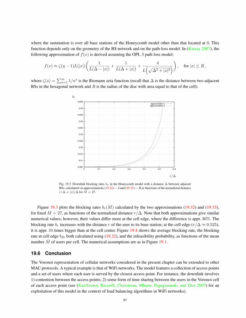
where the summation is over all base stations of the Honeycomb model other than that located at 0. Thisfunction depends only on the geometry of the BS network and on the path-loss model. In (Karray 2007), thefollowing approximation of f(x) is derived assuming the OPL 3 path loss model:

f(x) ≈ ζ(η − 1)L(|x|)(

1L(∆− |x|)

+1

L(∆ + |x|)+

4

L(√

∆2 + |x|2)) , for |x| ≤ R ,

where ζ(s) =∑∞

n=1 1/ns is the Riemann zeta function (recall that ∆ is the distance between two adjacentBSs in the hexagonal network and R is the radius of the disc with area equal to that of the cell).

br

0.005

0.01

0.015

0.02

0.025

0.03

0.035

0.04

0.045

0.05

0.055

0 0.1 0.2 0.3 0.4 0.5 0.6

approximation Iapproximation II

r/∆

Fig. 19.3 Downlink blocking rates bx in the Honeycomb model with a distance ∆ between adjacentBSs, calculated via approximations (19.32) — I and (19.33) — II as functions of the normalized distancer/∆ = |x|/∆ for M = 27.

Figure 19.3 plots the blocking rates br(M) calculated by the two approximations (19.32) and (19.33),for fixed M = 27, as functions of the normalized distance r/∆. Note that both approximations give similarnumerical values; however, their values differ more at the cell edge, where the difference is appr. 30%. Theblocking rate br increases with the distance r of the user to its base station; at the cell edge (r/∆ ≈ 0.525),it is appr. 10 times bigger than at the cell center. Figure 19.4 shows the average blocking rate, the blockingrate at cell edge bR, both calculated using (19.32), and the infeasibility probability, as functions of the meannumber M of users per cell. The numerical assumptions are as in Figure 19.1.

19.6 Conclusion

The Voronoi representation of cellular networks considered in the present chapter can be extended to otherMAC protocols. A typical example is that of WiFi networks. The model features a collection of access pointsand a set of users where each user is served by the closest access point. For instance, the downlink involves1) contention between the access points; 2) some form of time sharing between the users in the Voronoi cellof each access point (see (Kauffmann, Baccelli, Chaintreau, Mhatre, Papagiannaki, and Diot 2007) for anexploitation of this model in the context of load balancing algorithms in WiFi networks).

97

blocking rate, probability

0

0.1

0.2

0.3

0.4

0.5

0.6

0.7

0.8

0.9

1

20 25 30 35 40 45 50 55 60

averagecell edge

infeasibility

M

Fig. 19.4 Downlink average blocking rate: the blocking rate at the cell edge and the infeasibility prob-ability as functions of the mean number of users M per cell.

The main conclusion of the present chapter is that at least in the CDMA framework, power control can beintegrated into the spatial modeling tools advocated in this monograph. Power control can also be consideredwithin this frameworks for e.g. CSMA. However, there are very few mathematical results on power controlin infinite networks. For instance, consider the SINR graph of Definition 8.2.1 in Volume I. We recall that inthe basic SINR graph model, the transmission powers are constant. Consider a model where the SINR graphdoes not percolate for these constant transmission powers. Assume now that one can control the power ofeach transmitter so as to open certain links or so as to diminish the interference created by useless links. Wedo not know whether such a power control can let the SINR graph percolate when leaving all other networkparameters unchanged.

We showed in § 19.5 that the proposed approach extends to time–space scenarios and leads to spatialextensions of the classical loss model. This was exemplified through the Spatial Erlang formula establishedin Proposition 19.5.3. This was done for the constant bit rate (or SINR) scenario. The case of elastic traffic(where no minimal bit rate is required) can also be studied along the same lines. In this case, each arrival isassociated with some volume of data. The users of a BS are then all accepted and are served in a weightedprocessor sharing way; the weights determine bit-rates and are chosen in such a way that 1) the feasibilitycondition is satisfied; 2) some global utility function is maximized (see Chapter 11 in Volume I); the usersleave the system after having transmitted their data. For this case, explicit formulas for the mean throughputand the mean delay can be found in (Błaszczyszyn and Karray 2007).

98

Bibliographical Notes on Part IV

Chapter 16 follows (Baccelli, Blaszczyszyn, and Muhlethaler 2003) and (Baccelli, Blaszczyszyn, andMuhlethaler 2009a), where two-dimensional (2D) scenario is considered. The specificity of 1D scenario (inthe context of Linear Vehicular Ad-hoc NETworks (VANETs)) is explored in (Błaszczyszyn, Muhlethaler,and Toor 2009). Extensions of the analysis to the plain (non-slotted) Aloha and comparisons of to the slottedAloha in 2D scenario can be found in a forthcoming paper (Błaszczyszyn and Muhlethaler 2010).

Among other papers which have proposed methods allowing one to analyze coverage under generalfading conditions, let us quote (Hunter, Andrews, and Weber 2008), where one can find an analysis of theimpact of certain fading scenarios such as e.g. Nakagami. The formalism based on the Fourier L2 isometrywhich is developed in Chapter 16 and which allows one to cope with arbitrary fading (like e.g. Rician) wasproposed in (Baccelli, Blaszczyszyn, and Muhlethaler 2009a). Example 16.2.3 is borrowed from (Hunter,Andrews, and Weber 2008). Several papers have considered the evaluation of the mean throughput in thecontext of a Poisson MANET (e.g. (Ehsan and Cruz 2006) and (Haenggi 2009)). In (Ehsan and Cruz 2006),the authors evaluate the optimal SINR target T that a Poisson MANET using Spatial Aloha ought to usein order to maximize the mean throughput per unit area. The throughput is evaluated as the product of theprobability of coverage and the logarithm of 1 + T (Shannon’s capacity). This definition underestimates thereal throughput obtained by transmitters: given that transmission is successful, namely given that the actualSINR θ at the receiver is larger than T , the throughput is the logarithm of 1 + θ, which is larger than thelogarithm of 1+T . The approach developed in § 16.2.3 tells us how much larger, since we actually computethe distribution and the mean of the logarithm of 1 + θ. In (Haenggi 2009), closed form expressions arederived for specific fading scenarios.

Opportunistic Aloha was also considered in (Venkataraman and Haenggi 2004), where it was analyzedusing a Gaussian approximation for the interference, and in (Weber, Andrews, and Jindal 2007), where itwas called “threshold scheduling”. The exact analysis of opportunistic Aloha presented in § 16.4 is based on(Baccelli, Blaszczyszyn, and Muhlethaler 2009a).

Chapter 17 is primarily based on (Baccelli and Blaszczyszyn 2010). Formula (17.16) on the multicastcase is due to (Jacquet 2008). In relation with smallest hop in a cone, let us quote (Haenggi 2005), where a“n th-nearest-neighbor-in-a-cone” model is used to compare the efficiency of different routing schemes in a

99

Poisson MANET using ALOHA. The space-time scenario described in Section 17.5.1 will be used in Chap-ter 22 and allows one to address many important questions. In particular, it was introduced independently in(Ganti and M. 2009) to analyze the spatio-temporal correlation coefficient of slotted ALOHA.

When applied to Aloha, stochastic geometry can be used to analyze many other interesting problemswhich are not considered in Chapters 16 and 17, such as the optimal division of the available bandwidth intodifferent sub-bands (Jindal, Weber, and Andrews 2008) or power control to compensate for random fading(Jindal, Andrews, and Weber 2008).

The problem of infinite mean local delays observed in Section 17.5 is related to (Jelenkovic and Tan2007a; Jelenkovic and Tan 2007b), where it was shown that a finite population ALOHA model with variableand unbounded size packets has power law transmission delays (although the physical phenomena at handare quite different there and in our spatial MANET model with fixed-packet-sizes).

Chapter 18 follows (Nguyen, Baccelli, and Kofman 2007).The first part of Chapter 19 is based on (Baccelli, Błaszczyszyn, and Tournois 2003; Baccelli,

Błaszczyszyn, and Karray 2004). The feasibility probability was considered in different frameworks inin (Audrey M. Viterbi and Viterbi 1993), where it is called blocking probability and in (Liu and El Zarki1994) and (Evans and Everitt 1999), where it is called the outage probability. Section 19.5 follows (Baccelli,Błaszczyszyn, and Karray 2005). The authors of (Liu and El Zarki 1994) consider the blocking probability(as defined in this section) in a time–space framework and give simulation results which show that the feasi-bility and blocking probabilities are different in general. The time–space scenario considered in Section 19.5has several other incarnations: the case with elastic traffic is considered in (Błaszczyszyn and Karray 2007);the case with user mobility, which causes call cuts due to displacements, is analyzed in (Błaszczyszyn andKarray 2008a). In (Sidi and Starobinski 1997), explicit expressions of blocking probabilities are given fortwo limiting regimes: no mobility and infinite mobility. Further extensions can be found in (Błaszczyszynand Karray 2008b; Błaszczyszyn and Karray 2009). The whole approach is well summarized in (Karray2007).

100

Part V

Multihop Routing in Mobile ad HocNetworks

101

In this part, we study the performance of multihop routing in large MANETs. Readers not familiar withrouting can find some brief introduction to this topic in Part VI. The context is again that of a MANET ofthe Euclidean plane with randomly located nodes represented by a point process. The route followed bya packet is then is a random geometric object on this p.p., which depends on the routing algorithm whichis used. In this part, two main mathematical objects are introduced to describe and analyze these randomgeometric objects: the notion of point map on the p.p. of nodes, which can be seen as a way of describingthe routing algorithm, and the notion of route average, which allows one to define the statistics seen by apacket following the route.

Point Maps

Consider a locally finite set of points φ = {xi} of R2, for instance some realization of a Poisson p.p. A keyfeature of any routing scheme is that the next hop decision for a packet located at node X , and bound to theend destination D, should depend on D and X and not on where the packet comes from. Hence a routingmechanism to D can be defined through a point map on φ, namely a mapping A = AD : φ 7→ φ, whereA(X) is the next hop from node X . Let Ak denote the k-th iterate of A.

Definition. A point map A = AD on the pattern of points φ is a routing to destination D ∈ φ ifA(D) = D and, for all x ∈ φ, Ah(x) = D, for some finite h = h(x) ≥ 1.

Here are a few definitions related to such a routing.

• The smallest integer h = h(x) such thatAh(x) = D is the number of hops of the route from x toD; the latter is defined as the sequence of points p(x,D) =

(x,A(x),A2(x), . . . ,Ah(x) = D

).

• The vector J(x) = A(x)− x ∈ R2 is the jump vector from point x.• The real number P (x) = |x−D| − |A(x)−D| ∈ R is the progress to destination from point x.

Point Maps Associated with Graphs

Often, in addition to the node p.p., we have some underlying graph, where the vertices of the graph are thenodes and the edges represent the links which serve as a support to (or constraints for) the routing protocol.Let G = (φ, E) be such a graph, with E ⊂ φ × φ the set of (non-directed) edges. The elements of the setN (x) = {y ∈ φ : (x, y) ∈ E} will then be referred to as the neighbors of x ∈ φ.

Definition. A graph point map associated with the graph G = (φ, E) is a point map A on φ such that(x,A(x)) ∈ E for each x ∈ φ. In other words A(x) ∈ N (x), for all x ∈ φ.

Examples of graphs

Let φ be some realization of a homogeneous Poisson p.p. Φ; the following examples of graphs, with set ofnodes Φ, are pertinent for modeling multihop wireless communications and are used throughout this part:

• Poisson–Delaunay graph: in connection with Example 4.4.2 in Volume I, we call Poisson–Delaunay graph the graph GDelaunay = (Φ, EDelaunay) the edges of which are the sides of theDelaunay triangles generated by the Poisson p.p. Φ (cf. Definition 4.4.1 in Volume I). Recall that

102

the edges EDelaunay = {(x, y) : x ∈ Φ, y ∈ Nx(Φ)} of this graph connect each point x ∈ Φ ofthe Poisson p.p. to all its Voronoi neighbors Nx(Φ) (cf. Lemma 4.4.3 in Volume I). This graphis very convenient in that it is almost surely connected. Its main weakness within the presentcontext is the lack of realism of Delaunay edges for representing wireless links.• Random geometric graph: this is the Boolean connectivity graph, obtained when having an

edge between two points of the Poisson p.p. iff the distance between them is less than somethreshold Rmax. In the wireless setting, this graph is often referred to as the transmission rangegraph. Here, the neighborhood depends not only on the geometry of the p.p. but also on theparameter Rmax, which is often used to model the maximal transmission range of a wirelessnode (e.g. taking Rmax = max{r : P/l(r) ≥ Po}, where P is the power of the transmitter,l(r) some OPL function and Po is the minimal detection power). This model is equivalent to theconnectivity graph of the Boolean Model (BM) with spherical grains of deterministic radius. Themain problem with this model is that the graph on the whole plane is not connected (more pre-cisely, it is disconnected with probability 1; cf. Proposition 3.2.4 in Volume I). This means that,on this graph, routing is only possible between points of Φ which belong to the same connectedcomponent. A natural idea is to assume that the BM percolates and to consider routing on theunique infinite connected component of the BM (cf. Section 3.2.2 in Volume I). This howeverconsiderably complicates the analysis.• Connected component of the SINR graph: A more pertinent but more complicated model is the

SINR connectivity graph GSINR (see Definition 8.2.1 in Volume I). Recall that for the M/DW+M/D

model, this graph percolates (cf. Section 8.3 in Volume I) and one can consider routing on itsgiant component. 3

Spatial Averages and Route Averages — Routing Paradox

Our main objective within this framework is the analysis of various classes of routing algorithms, whenoperated on Poisson p.p. For all routing algorithms, we are particularly interested in route averages andspatial averages, defined below and on fluctuations around these averages. It is customary to fix the originof the plane O at the destination node D and to consider routing A = AD = AO to the origin of the plane.Let g be some function from R2 to R.

• The route average of g w.r.t. point map A is defined as

r = lim|x|→∞

1h(x)

h(x)−1∑k=0

g(Ak+1(x)−Ak(x)) ,

whenever the last a.s. limit exists and is independent of the direction with which x tends to∞. This definition requires a subsequence of points of Φ which tends to infinity in some fixeddirection; this will be made precise when needed (see e.g. Definition 20.3.1). In this definition,h(x) is the number of hops of the A-route from x to O. For instance, if g(x) = |x|, r is the routeaverage of the jump size.• The spatial average of g w.r.t. the point map A is defined as

s = limρ→∞

1|φ(BO(ρ))|

∑x∈φ∩BO(ρ)

g(A(x)− x)) ,

3It is natural to conjecture that the infinite component of this graph is unique, provided it exists; we are not aware of any published proof of this fact.

103

whenever the last almost sure limit exists. In this definition, BO(ρ) is the ball of center O andradius ρ.

As we shall see, these two types of averages do not coincide in general. This observation belongs to theclass of Palm biases and continues in a sense Feller’s paradox. Feller’s paradox is concerned with stationaryp.p. on the real line (interpreted as time below). The paradox is that statistics made by an observer, whichmeasures the length of the interval that separates time t to the first point of the p.p. after t, in general differwhen t is an arbitrary instant of time (say 0) and when it is the typical point of the p.p.

In the same vein, one can obtain different statistics on e.g. the jump vector associated to a point map A,when this jump is taken from a typical point of the point pattern and when it is taken from the typical pointof some (long) route prescribed by the very same point map A. By analogy, this will hence be called therouting paradox.

The Price of Anarchy in Routing

Another key concern is the price of anarchy within this setting. For most kinds of routing paradigms, onecan define both optimal and greedy versions. The optimal schemes are all based on dynamic programming;they often come with heavy computational and state construction overheads which are problematic in thiswireless and infrastructure-less MANET context. Suboptimal and in particular greedy versions, which arebased on local optimizations and require less exchange of information are often preferred as they come witha much smaller computational cost. Locality can be either in time or space depending on the cases. The mainquestion is then the quantification of the loss of performance between optimal and greedy solutions, whichit is then natural to be baptized price of anarchy (in routing). This price is analyzed in terms of the spaceand route averages alluded to above.

Structure of Part V

Chapter 20 studies optimal (shortest path or minimal weight) routing. Chapter 21 is focused on greedynear-neighbor routing. These two first chapters focus on routes which are made of a collection of adjacentand feasible links seen in a snapshot of the network. In these two chapters, we consider conventional routingprotocols (like e.g. shortest path routing); in these conventional schemes, when a route is determined betweenan origin and a destination, this route remains the same as long as the network nodes do not move and linksremain stable; once the route is determined, the MAC is then used to let packets progress from origin todestination along this route. This allows one to separate the routing problem from the MAC protocol.

In Chapter 22, we study time-space routing where the next relay on the route to the destination changesfrom a packet to the next and where the next hop is selected among the nodes having successfully receivedthe packet (if any), which again depends on the SINR at the receivers. Such a scheme allows one to takeadvantage of the local pattern of transmissions as determined by the MAC and by the fading variables, ateach hop and at each time. Within this context, one can again define both optimal and greedy versions. Oneof the important objects within this framework is Opportunistic routing, a greedy algorithm where, at eachtime slot, each node selects the best relay to route the packet towards its end destination. By best, we meane.g. the relay which maximizes the progress of the packet towards the destination. These SINR-based routingschemes are analyzed in terms of random and time-space point maps.

104

20Optimal Routing

20.1 Introduction

This chapter is focused on optimal multihop routing on (weighted) graphs associated with stationary pointprocesses of the Euclidean plane and in particular Poisson point processes. We focus on the existence andthe evaluation of route averages. More precisely, we establish a generic scaling law which shows that for alarge class of optimal routing schemes, which includes shortest path and minimal weight routing on suchgraphs, the length (or weight) of the optimal path is asymptocically linear in the distance between sourceand destination. The main tool used here is the sub-additive ergodic theorem. The main technicalities bearon proving that the constants in the sub-additive ergodic theorem are not degenerate.

20.2 Optimal Multihop Routing on a Graph

Weights. Consider a locally finite pattern of points φ =∑

i εxi on R2. Consider a graph G = (φ, E) onthis point pattern and assume some non-negative weightsw(x, y) to be associated with each edge (x, y) ∈ E .The following examples of weights are of interest: for y ∈ N (x),

• Graph distance: w(x, y) = wgraph(x, y) = 1;• Euclidean distance: w(x, y) = wEuclid(x, y) = |x − y| (more generally one can considerwα(x, y) = |x− y|α, for some 0 ≤ α <∞);• Random weights e.g. w(x, y) = w(y, x) are i.i.d. random variables.

When a marked pattern of points is considered, more elaborate weights can be contemplated. For instance,consider a standard stochastic scenario for a SN of the M/GI type. For all pairs of points x, y ∈ Φ, letIx,y(.) denote the SN generated by Φ \ {x, y}. Then, in the wireless context, it is natural to consider e.g.w(x, y) = max(Ix,y(x), Ix,y(y)). Another natural example related to the digital communication modelframework is that where the weight of a link is the bidirectional delay of this link, namely

wdelay(x, y) = max

((log(

1 +F yx /l(|x− y|)W + Ix,y(y)

))−1

,

(log(

1 +F xy /l(|x− y|)W + Ix,y(x)

))−1), (20.1)

105

where F yx is the fading from x to y.It is often convenient to extend the definition of weights to all pairs of nodes (x, y) ∈ φ2 by taking

w(x, y) =∞ for y 6∈ N (x).

Optimal Paths. Consider the collection of all paths π of G = (φ, E) between S and D. Each of them isa sequence of the form x1, . . . , xn with n integer, x1 = S and xn = D. Pick some non-negative weightfunction w and define the weight of π as

|π| =n−1∑i=1

w(xi, xi+1) .

We define p∗(S,D) to be the minimal weight path in this collection.Note that it is not guaranteed that such an optimal path exists (at least on an infinite collection of nodes).

However, if φ is locally finite (recall that the realizations of a point process are a.s. locally finite by defini-tion), then a minimal weight path always exists for wgraph or wEuclid. Even if we have existence, uniquenessis not guaranteed. When existence is granted, the collection of minimal weight paths satisfy the dynamicprogramming equation

|p∗(x,D)| = miny∈N (x)

(w(x, y) + |p∗(y,D)|) . (20.2)

Dijkstra’s algorithm (see § 25.3.1.2) uses this to recursively build the optimal paths. Whenever the argminis almost surely uniquely defined for all x, so is the optimal path from S to D. This is the case for wEuclidbut not for wgraph.

Assume uniqueness is granted. Then it follows from the dynamic programming equation that if bothp∗(S,D) and p∗(S′, D) contain node x, then the subpaths of p∗(S,D) and p∗(S′, D) from x to D coincide(and are equal to p∗(x,D)). Hence, under the above existence and uniqueness assumptions, there is a pointmap associated with minimal weight paths to D and this point map is a routing to D.

We have similar results in case we have no uniqueness (e.g. for wgraph). Let P ∗(S,D) denote the col-lection of optimal paths from S to D. Assume that x belongs to some paths of P ∗(S,D) and of P ∗(S′, D).Then the collection of all subpaths of P ∗(S,D) from x toD coincides with that of all subpaths of P ∗(S′, D)from x to D and with P ∗(x,D). In order to define a point map in this case, it is enough to select one of thepaths of P ∗(S,D) in an appropriate way (e.g. the one with minimal Euclidean distance).

Definition 20.2.1. Let D be some destination in φ. We call minimal weight routing (MWR) and denote byA∗ = A∗D the point map associated with the minimal weight path.

If the weights are wgraph or wEuclid, MWR is often referred to as shortest path routing. Note that for allroutings A to D on (φ, E), for all x ∈ φ,

|p∗(S,D)| =h∗(x)∑i=1

w(A∗i−1(x),A∗i(x)

)≤

h(x)∑i=1

w(Ai−1(x),Ai(x)

). (20.3)

Here h(x) (resp. h∗(x)) is the number of hops from x to D in A (resp. A∗).

106

20.3 Asymptotic Properties of Minimal Weight Routing

In this section, we assume that the random graph G = (Φ, E) is jointly stationary with its edge weightsw(xi, yi); i.e. the distribution of the triple G = (Φ, E , w(·)) is the same as that of G + a = (Φ + a, E +a,w(· + a)), for all a ∈ R2, where (x, y) + a = (x + a, y + a) is the shifting of the edge (x, y) ∈ E bythe vector a. This holds for all the instances of weights considered above. We also assume that Φ is a simplep.p. and a/the MWR A∗(w,D) almost surely exists, for all destinations D ∈ Φ. If we have no uniqueness,we assume that |p∗(xi, xj)| is uniquely defined, almost surely for all xi, xj ∈ Φ.

By asymptotic property, we mean here the behavior of the total weight of the optimal route betweentypical points of Φ when the Euclidean distance between them tends to infinity.

The appropriate way of defining ”typical” points xi, xj ∈ Φ that are more and more distant is based onan extension of the notion of routing to routing from s to t, where s, t are not necessarily points of Φ. ByLemma 4.2.2 in Volume I, for all t ∈ R2, the point of Φ which is the nearest to t, which is denoted by x(t)below, is almost surely uniquely defined.

Definition 20.3.1. The MWR to t ∈ R2 w.r.t. (Φ, E , w), where t is not necessarily a point of Φ, is definedas the MWR A∗x(t), w.r.t. (Φ, E , w), to the point x(t) ∈ Φ. The MWR route p∗(s, t) from s ∈ R2 to t ∈ R2

is defined as the optimal route p∗(x(s), x(t)) from x(s) ∈ Φ w.r.t. A∗x(t).

In order to underline the fact that p∗(s, t) depends on the realization of G not only through x(s), x(t) andall other points of Φ, but also through the realizations of the weights if the latter are random, we sometimesuse the notation p∗(s, t, G).

First principles show that the family of minimal weight routes p∗(s, t), s, t ∈ R2, satisfies the followingsubadditivity property:

Lemma 20.3.2. Assume that MWR routes are almost surely well defined between all pairs of points s, t ∈R2. Then for all s, t, v ∈ R2

|p∗(s, t, G)| ≤ |p∗(s, v, G)|+ |p∗(v, t, G)| .

We are now in a position to prove the following general result.

Theorem 20.3.3 (Kingman’s subadditive theorem). Assume that G = (Φ, E , w) is stationary with non-negative edge weightsw(·, ·) and suppose that |p∗(xi, xj , G)| is almost surely well-defined for all xi, xj ∈ Φ.For all vectors d ∈ R2 with |d| = 1 and such that

E[|p∗(0, d, G)|] <∞, (20.4)

the limitlimγ→∞

γ−1E[|p∗(0, γd, G)|] = infγ>0

γ−1E[|p∗(0, γd, G)|] = κd (20.5)

exists with κd <∞. If moreover

E[

supγ1<γ2,γ1,γ2∈I

|p∗(γ1d, γ2d, G)|]<∞ , (20.6)

107

for some non-degenerate finite interval I ⊂ R, then the following limit exists almost surely

Kd = limγ→∞

γ−1|p∗(0, γd, G)| (20.7)

and E[Kd] = κd.

Proof. The result follows from Lemma 20.3.2 and the continuous-parameter sub-additive ergodic theorem(see (Kingman 1973, Theorem 4)).

Remark: If G is motion invariant (stationary and rotation invariant), then the distribution of Kd does notdepend on the direction d.

If G = (Φ, E , w) is stationary and ergodic (cf. Definition 1.6.7 in Volume I and Proposition 1.6.10 inVolume I), then the random variable Kd is constant and equal to κd (i.e. it does not depend on the realizationof G).

If G = (Φ, E , w) is motion invariant and ergodic, then κd ≡ κ.

20.3.1 MWR on the Poisson–Delaunay Graph

Consider the Poisson–Delaunay graph GDelaunay = (Φ, EDelaunay) defined in Example 4.4.2 in Volume I.On GDelaunay, the shortest Euclidean distance paths are almost surely well defined. The same does not holdtrue for the minimal number of hop routing; however the minimal number of hops |p∗(S,D)| required to gofrom S to D is uniquely defined (cf. Corollary 25.3.2).

Proposition 20.3.4. Consider the Delaunay graph GDelaunay = (Φ, EDelaunay, w), on some homogeneousPoisson p.p. Assume edges are independently marked by non-negative random weights w(x, y) = w(y, x)with distribution function F . Then MWR routing on this graph satisfies (20.5) and (20.7) with 0 ≤ Kd =κd = κ <∞ if and only if

E[min(w1, w2, w3)] =

∞∫0

(1− F (u))3 du <∞ , (20.8)

where wi are independent copies of the generic weight.

We sketch the main line of the proof (given in (Vahidi-Asl and Wierman 1990)), which is based on thefollowing fact concerning the site-percolation model (cf. (Russo 1987)).

Lemma 20.3.5. Consider a super-critical site percolation model on the square lattice. LetB be a finite set ofsites. Denote by C the smallest open circuit aroundB (which exists with probability one in the super-criticalregime) and by N the number of sites surrounded by C. Then E[Nα] <∞ for all α > 0.

Proof. [of Proposition 20.3.4] Fix two points, say 0, t ∈ R2. We first show that for all t, E[|p∗(0, t)|] <∞.For this, consider a square-lattice of side length A and associate a site with each square. It is not difficult toshow that if each site of some given circuit of sites is “densely populated” by points of the Poisson p.p. Φ,then one can find two disjoint circuits in the Poisson–Delaunay graph of Φ which are covered by this circuitof sites (cf. Figure 20.1 and see (Vahidi-Asl and Wierman 1990) for details).

108

A

C

H

A

B t0

Fig. 20.1 Three disjoint paths of the Delaunay graph connecting 0 to t.

The probability that a given site is “densely populated” tends to 1 when A tends to ∞. Thus, for Alarge enough, this probability is larger than the critical site-percolation probability. From now on, fixA largeenough for this to hold.

Let B be the smallest rectangular set of sites covering the interval [0, t]. Denote by C the smallestcircuit of “densely populated” sites around B and by H the set of sites surrounded by C. Since both pointsx(0) ∈ Φ and x(t) ∈ Φ have (at least) three neighbors in the Delaunay graph, it is possible to find (at least)three disjoint paths on this graph connecting x(0) to x(t), which lay in C ∪H (cf. Figure 20.1). Call thesepaths pi, i = 1, 2, 3. We have

E[|p∗(0, t)|] ≤ E[ mini=1,2,3

|pi|] =∞∑k=0

P{ mini=1,2,3

|pi| > k } =∞∑k=0

(P{ |p1| > k }

)3.

Denote by L the number of hops and byw1, . . . , wL the weights of the edges of p1. We have |p1| =∑L

i=1wiand

P{ |p1| > k |L = l} ≤l∑

i=1

P{wi > k/l } ≤ l(1− F (k/l)) .

Thus

E[|p∗(0, t)|] ≤ E[L3

∞∑k=0

(1− F (k/L))3

]≤ E[L3] + E[L4]

∞∫0

(1− F (u))3 du ,

and in order to conclude the proof, it remains to prove that E[L4] <∞.Since p1 ⊂ C∪H , and the path p1 can be taken without loops, we have L ≤ Φ(C∪H) =

∑Nn=1 Φ(∆n),

where ∆n are the sites ofC∪H andN is the number of sites inC∪H . Note that the random variables Φ(∆n)are neither i.i.d. nor Poisson distributed because they are defined from the circuit of “densely populated” sitesC. However, when considering all possible values for the set C ∪H , we get

E[L4] =∞∑n=1

∑K=D1∪...∪Dn

E[L4 1(C ∪H = K)]

≤∞∑n=1

∑K=D1∪...∪Dn

E[( n∑

i=1

Φ(Di))41(C ∪H = K)

],

109

where the summation is over all possible finite configurations K of n sites Di, i = 1, . . . , n. Note thatC ∪H = (C ∪H)(Φ) is a stopping set with respect to Φ (see Definition 1.5.1 in Volume I). More precisely,for any bounded setK =

∑ni=1Di, whereDi are fixed sites, one can check whether the event {C∪H(Φ) =∑n

i=1Di } holds or not knowing only which sites Di, i = 1, . . . , n, are “densely populated”. Moreover, forany given site D,

E[(Φ(D))4 |D is not “densely populated”] ≤ E[(Φ(D))4]

≤ E[(Φ(D))4 |D is “densely populated”] ≡ m0 <∞ ,

for some constant m0. Thus

E[L4] ≤∞∑n=1

∑K=D1∪...∪Dn

E[( n∑

i=1

Φ(Di))41(C ∪H = K)

]≤

∞∑n=1

∑K=D1∪...∪Dn

n4m40E[1(C ∪H = K)

]= m4

0E[N4] <∞ ,

where the last inequality follows from Lemma 20.3.5. This completes the proof that E[|p∗(0, t)|] <∞. Now,in order to obtain the result for the supremum E[supu,v∈[0,t] |p∗(u, v)|] < ∞ as required in (20.6), one canconsider the sum of all the lengths of the minimal paths from any point u to any v, both in the interval [0, t].Using similar arguments as above and noting that the number of couples x(u) and x(v) does not exceed N2

one can conclude the result from the fact that E[N6] <∞.

Note that the constant κ in Proposition 20.3.4 can be null. Intuitively κ > 0 provided the weights ware not too small. For addressing this question, consider the independent bond percolation model on thePoisson–Delaunay graph GDelaunay, namely the model where each bond (edge of GDelaunay) is open orclosed independently of everything else. Denote by An the event that there is an open horizontal crossing ofthe rectangle [0, 3n]× [0, n] in this model. Let η∗(p) = lim infn→∞Pp{An}, where Pp denotes the law ofthe model where the probability that a bond is open is p. Finally, denote by p∗c = inf{p > 0 : η∗(p) = 1}.1The following result was proved in (Pimentel 2006).

Proposition 20.3.6. Under assumption (20.8), if F (0) < 1 − p∗c , then the constant κ in Proposition 20.3.4satisfies 0 < κ <∞.

Since the metric wgraph is equivalent to w(x, y) ≡ 1, for all (x, y) ∈ EDelaunay, and since it obviouslysatisfies condition (20.8) and F (0) = 0, we have:

Corollary 20.3.7. For the metric wgraph, 0 < κgraph <∞.

We now focus on the Euclidean metric. Some realization of the Euclidean shortest path route is depictedin Figure 20.2.

1It is shown in (Pimentel 2006) that p∗c ≥ 1−pc, where pc is the critical probability for the independent bond percolation on the Poisson–Delaunaygraph GDelaunay . Moreover, it is conjectured that pc + p∗c = 1.

110

Proposition 20.3.8. Consider the homogeneous Poisson–Delaunay graph GDelaunay = (Φ,EDelaunay, wEuclid) with Euclidean weights. The shortest path on this graph satisfies (20.5) and (20.7) with1 ≤ Kd = κd = κ ≤ 2π

3 cos(π/6) <∞.

The above result can be proved using the following fact from (Keil and Gutwin 1992).

Lemma 20.3.9. Given any finite set φ of points on the plane. For any two points x, y ∈ φ, the Euclideanshortest path p∗(x, y) satisfies

|p∗(x, y)||x− y|

≤ 2π3 cos(π/6)

≈ 2.42 .

Proof. [of Proposition 20.3.8]. Fix two points, say 0, t ∈ R2. One can find a bounded set G = G(Φ), largeenough so as to have p∗(0, t,Φ) = p∗(0, t,Φ ∩G(Φ)). For example G = C ∪H as defined in the proof ofProposition 20.3.4. By Lemma 20.3.9

|p∗(0, t)| = |p∗(0, t,Φ ∩G(Φ))| ≤ 2π3 cos(π/6)

|x(0)− x(t)|

andsups∈[0,t]

|x(0)− x(s)| ≤ t+ 2|x(t/2)− t/2| .

Using the stationarityE[|x(t/2)− t/2|] = E|x(0)|] <∞ .

To justify the upper bound on κ note that

κ ≤ lim|t|→∞

2π3 cos(π/6)

E[|x(0)− x(t)|]|t|

≤ 2π3 cos(π/6)

(1 + lim

|t|→∞

E[|x(0)|]|t|

+ lim|t|→∞

E[|x(t)− t|]|t|

)=

2π3 cos(π/6)

(1 + 2 lim

|t|→∞

E[|x(0)|]|t|

)=

2π3 cos(π/6)

.

For the lower bound on κ, one can use the triangle inequality to obtain |p∗(x(0), x(t)| ≥ |x(0)− x(t)| and

|p∗(0, t)||t|

=|p∗(x(0), x(t)|

|t|≥ |x(0)− x(t)|

|t|≥ 1− |x(0)|

|t|− |x(t)− t|)

|t|.

Thus by (20.5)

κ ≥ 1− lim|t|→∞

(E[|x(0)|]|t|

− E[|x(t)− t|])|t|

)= 1− 2 lim

|t|→∞

E[|x(0)|]|t|

= 1 .

Remark: The conditions ensuring the non-degeneracy of the constant κdelay associated with minimal delayrouting are not known as to the writing of this monograph.

111

0.40.2-0.2-0.4

0.15

0.1

0.05

0

-0.05

-0.1

-0.15

Fig. 20.2 Euclidean shortest path routing on the Poisson–Delaunay graph.

20.3.2 Scale Invariance of the Poisson–Delaunay Subadditive Constants

We now study the scale invariance properties of the Poisson–Delaunay subadditive constants κgraph, κEuclidwith respect to the intensity λ of the underlying Poisson p.p. Recall that if Φ = {xi} is a realization of thePoisson p.p. of intensity λ = 1, then Φ(λ) = {xi/

√λ} is a realization of the Poisson p.p. of intensity λ

(cf. Example 1.3.12 in Volume I). Moreover, if p∗(s, t,Φ) = (x1, . . . , xk) is a shortest path from s to ton GDelaunay(Φ, EDelaunay), then p∗(s, t,Φ)/

√λ = (x1/

√λ, . . . , xk/

√λ) is a shortest path from s/

√λ to

t/√λ on the Delaunay graph generated by Φ(λ). Thus, for wEuclid, we have

|p∗Euclid(s/√λ, t/√λ,Φ(λ))| = |p∗Euclid(s, t,Φ)|/

√λ

and for wgraph, we have|p∗graph(s/

√λ, t/√λ,Φ(λ))| = |p∗graph(s, t,Φ)|.

Consequently for the Euclidean shortest path routing, the ergodic constant does not depend on λ since

κEuclid(λ) = lim|t|→∞

1/|t||p∗Euclid(0, t,Φ(λ)|

= lim|t|→∞

√λ/|t||p∗Euclid(0, t,Φ)|/

√λ

= κEuclid(1) = κEuclid , (20.9)

whereas for the graph distance shortest path routing,

κgraph(λ) = lim|t|→∞

1/|t||p∗graph(0, t,Φ(λ)|

= lim|t|→∞

√λ/|t||p∗graph(0, t,Φ)|

=√λκgraph(1) . (20.10)

We say that that the Euclidean shortest path routing on the Poisson–Delaunay graph approximates theEuclidean distance with a constant stretch of κEuclid. Simulations show that κEuclid is approximately equalto 1.05.

20.3.3 MWR on the Random Geometric Graph

As already mentioned, the random geometric graph has a positive fraction of isolated nodes for all transmis-sion ranges r. Nevertheless, the MWR path between two nodes is well defined when adopting the convention

112

that the weight between two nodes which are not connected by an edge have a fictitious edge with an infiniteweight. When the connectivity range is such that the associated random geometric graph percolates, thenone can consider the MWR between nodes of the infinite connected component of this graph. Letting X(t)denote the node of this infinite component which is the closest to t, where t ∈ R2 and p∗(s, t) the MWRpath from X(s) to X(t), then for all s, t and v ∈ R2,

|p∗(s, t)| ≤ |p∗(s, v)|+ |p∗(v, t)| .

Hence, the linear scaling of (20.7) holds in this case too provided the integrability condition (20.4) holds.

20.3.4 MWR on the SINR Graph

By the same argument as above, when the bidirectional SINR graph GSINR of Definition 8.2.1 in Volume Ipercolates, then the same subadditive inequality holds and this implies a linear scaling of the optimal pathsunder a condition of the type (20.4).

20.4 Largest Bottleneck Routing

One may think of a routing which realizes the optimality principle expressed in Definition 20.2.1 but withthe sum of the weights

∑ki=1w(. . .) replaced by the maximum weight, namely for all routings A to D on

(φ, E), for all x ∈ φ,

h∗(x)maxi=1

w(A∗i−1(x),A∗i(x)

)≤

h(x)maxi=1

w(Ai−1(x),Ai(x)

). (20.11)

For example, if the weight wdelay(x, y) is the inverse of the throughput of the link as defined in (20.1)), sucha routing would select paths with the largest possible (throughput) bottleneck.

Remark: Note that the question whether there exists a path between two given points with all its weightssmaller than a given threshold is in fact a percolation question. If the weights are the inverse of throughputas defined in (20.1), then this boils down to the SINR percolation model studied in Chapter 8 in Volume I.

20.5 Optimal Multicast Routing on a Graph

Consider a finite point pattern φ with an underlying weighed graph (φ, E , w) The optimal multicast tree ofthis point pattern is the minimal weight spanning tree on this graph (see Chapter 13 in Volume I). If thegraph is the complete one and the weight is wEuclid, this is the MST (see § 3.2 in Volume I).

20.6 Conclusion

We shall revisit optimal paths in Chapter 22 in the context of time–space routing. However, in the wirelesscontext, a major drawback of all these classes of optimal routing schemes is the large overhead associatedwith the evaluation of the routing table: in order to determine A∗D(x), the neighbor of node x to which apacket with destination D should be sent, Dijkstra’s algorithm requires that node x discover node D (cf. thelast remark in § 25.3.1.2). Of course this search can be organized in a distributed way by exchanging infor-mation between neighbors as indicated in § 25.3.1.2, but it terminates only after all the paths originating fromx and of weight smaller than |p∗(x,D)| have been discovered (cf. the last statement of Proposition 25.3.1).Moreover, when the topology changes somewhere in the network, the algorithm has to be restarted, which is

113

quite problematic in a mobile network. This explains the interest of the networking community in subopti-mal but locally defined paths such as those considered in the next chapter and at the end of Chapter 22. Theloss in performance due to suboptimality being often more than compensated by the reduction in routingtable overhead.

114

21Greedy Routing

21.1 Introduction

The present chapter is focused on greedy geographic routing. By greedy, we mean that we replace globaloptimality as considered in the last chapter by local (and hence sub-optimal or greedy decisions). The localdecisions of a given node are based on the exchange of location information with its neighbors only (hereagain, we assume the existence of some underlying graph allowing one to define neighborhoods). Hence theterm ’geographic’.

Among the drawbacks of this class of algorithms, let us first quote the fact that they are only applicable tonetworks of nodes located in the Euclidean plane (or space); in addition, these algorithms require that nodeshave some knowledge of their position, and also that the position of the destination be known. Finally, theyare sub-optimal. But all this is compensated by the fact that the overhead associated with the construction ofthe routing table vanishes.

In the present chapter, we first list a few basic geographic routing algorithms and their associated pointmaps (§ 21.2). We study a couple of them. The first one, next-in-strip routing, is a toy example which consistsin using the nodes located in a strip containing the source and the destination as relays. In the second one,smallest hop routing, the next relay is the node which is the closest among those which are closer to thedestination. The rationale, which was already mentioned in Chapter 16, is that it is in a sense best to favorhops to the nearest neighbors.

The main results of the analysis consist of spatial averages which are obtained using new types ofstochastic geometry arguments (§ 21.4), and route averages, which are based on Markovian analysis (§ 21.7).

A key observation is that these two types of averages do not coincide in general. In the smallest hop case,the latter has better performance than the former.

In addition to point-to-point routes, we also consider the multicast (either one-to-many or many-to-one)case. For this, we use the spanning trees that are obtained by taking the union of greedy routes to somecommon destination and which we call radial spanning trees (RST). These spanning trees can be usedeither on a large population of nodes as considered in § 21.5 (e.g. for diffusion in a MANET), or in a meshor a sensor network context, where the main problem consists in building a collection of ’small spanning

115

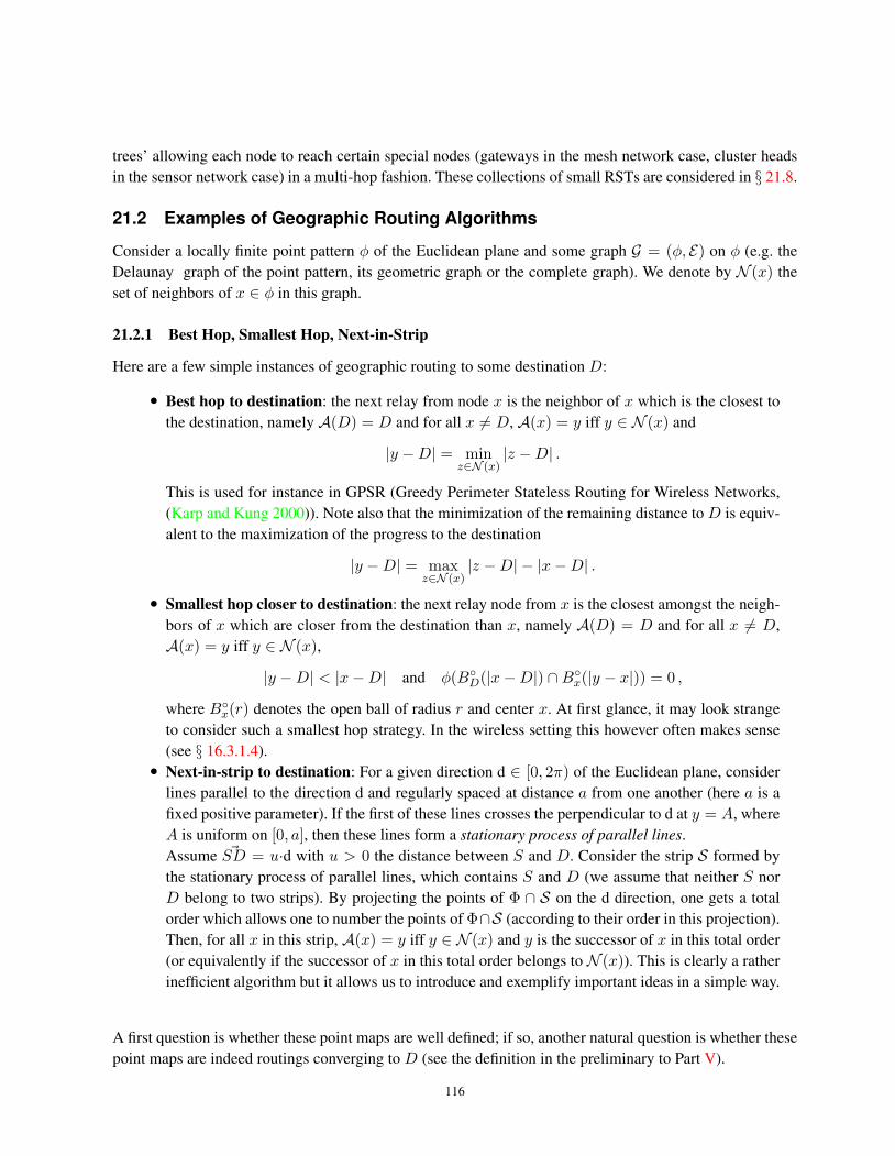
trees’ allowing each node to reach certain special nodes (gateways in the mesh network case, cluster headsin the sensor network case) in a multi-hop fashion. These collections of small RSTs are considered in § 21.8.

21.2 Examples of Geographic Routing Algorithms

Consider a locally finite point pattern φ of the Euclidean plane and some graph G = (φ, E) on φ (e.g. theDelaunay graph of the point pattern, its geometric graph or the complete graph). We denote by N (x) theset of neighbors of x ∈ φ in this graph.

21.2.1 Best Hop, Smallest Hop, Next-in-Strip

Here are a few simple instances of geographic routing to some destination D:

• Best hop to destination: the next relay from node x is the neighbor of x which is the closest tothe destination, namely A(D) = D and for all x 6= D, A(x) = y iff y ∈ N (x) and

|y −D| = minz∈N (x)

|z −D| .

This is used for instance in GPSR (Greedy Perimeter Stateless Routing for Wireless Networks,(Karp and Kung 2000)). Note also that the minimization of the remaining distance to D is equiv-alent to the maximization of the progress to the destination

|y −D| = maxz∈N (x)

|z −D| − |x−D| .

• Smallest hop closer to destination: the next relay node from x is the closest amongst the neigh-bors of x which are closer from the destination than x, namely A(D) = D and for all x 6= D,A(x) = y iff y ∈ N (x),

|y −D| < |x−D| and φ(B◦D(|x−D|) ∩B◦x(|y − x|)) = 0 ,

where B◦x(r) denotes the open ball of radius r and center x. At first glance, it may look strangeto consider such a smallest hop strategy. In the wireless setting this however often makes sense(see § 16.3.1.4).• Next-in-strip to destination: For a given direction d ∈ [0, 2π) of the Euclidean plane, consider

lines parallel to the direction d and regularly spaced at distance a from one another (here a is afixed positive parameter). If the first of these lines crosses the perpendicular to d at y = A, whereA is uniform on [0, a], then these lines form a stationary process of parallel lines.Assume ~SD = u·d with u > 0 the distance between S and D. Consider the strip S formed bythe stationary process of parallel lines, which contains S and D (we assume that neither S norD belong to two strips). By projecting the points of Φ ∩ S on the d direction, one gets a totalorder which allows one to number the points of Φ∩S (according to their order in this projection).Then, for all x in this strip, A(x) = y iff y ∈ N (x) and y is the successor of x in this total order(or equivalently if the successor of x in this total order belongs to N (x)). This is clearly a ratherinefficient algorithm but it allows us to introduce and exemplify important ideas in a simple way.

A first question is whether these point maps are well defined; if so, another natural question is whether thesepoint maps are indeed routings converging to D (see the definition in the preliminary to Part V).

116

21.2.2 Geographic Routing on a Poisson Point Process

In this section, we address the last questions when φ is some realization of a homogeneous Poisson p.p. Φ,under its Palm distribution, namely with an additional point at D.

Random Geometric Graph. On the random geometric graph, with a positive probability, the setN (x) is∅ (or {x} depending on the convention), Hence, on this graph, none of these point maps are routings in thatthere exists a positive fraction of the nodes for which these point maps do not converge to the destination.

One natural solution is to assume that the random geometric graph percolates (see § 3.2 in Volume I)and to limit the ambitions of routing to (source and destination) nodes which belong to the infinite compo-nent. However, this does not work either due the following dead end problem: consider any of the routingmechanisms described above (best hop, smallest hop or next-in-strip to destination D). Even if we assumethat there is a path of the random geometric graph between S and D, the geographic routing algorithm mayreach a dead end node, namely a node X such that all neighbors of X in the random geometric graph aremore distant from D than X . Let us look at what then happens:

• If we take the convention that x /∈ N (x) for all x, then smallest hop routing and next-in-striprouting are undefined at X . For best hop, assume for instance that X was first reached from nodeY and that A(X) = Y ; then best hop reaches a limit cycle Y,X, Y,X, . . ..• If we take the convention that x ∈ N (x) for all x, then smallest hop and next-in-strip are again

ill defined at X whereas best hop stop at X and remains there.

Hence, because of the dead end problem, these algorithms may not converge to the destination when usedon the random geometric graph.

Poisson Delaunay Graph.

Lemma 21.2.1. For all D and x, the set N (x) ∩B◦D(|x−D|)) is almost surely non-empty.

Proof. IfD belongs toN (x), thenD ∈ N (x)∩B◦D(|x−D|)). IfD /∈ N (x), then x lies oustide the Voronoiflower of point x w.r.t φ. Consider the Voronoi tessellation of the finite point pattern {x} ∪ N (x). In thistessellation, x has the same Voronoi flower as in that w.r.t. φ. Since the Voronoi flower contains the Voronoicell, D belongs to at least one of the infinite Voronoi cells of the points of the set N (x). That is, there is (atleast) a point of N (x) closer to D than x.

Using this and the fact that the probability that there are two points at the same distance from x is zero, weget that the point map is almost surely well and uniquely defined for both best and smallest hop routing. Inaddition

Proposition 21.2.2. On the Poisson-Delaunay graph, both best and smallest hop point maps are well definedroutings.

Proof. From the last lemma, either the next hop is D or the distance to D decreases. Since Poisson pointpatterns are almost surely locally finite, each point map leads to D in a finite number of steps.

117

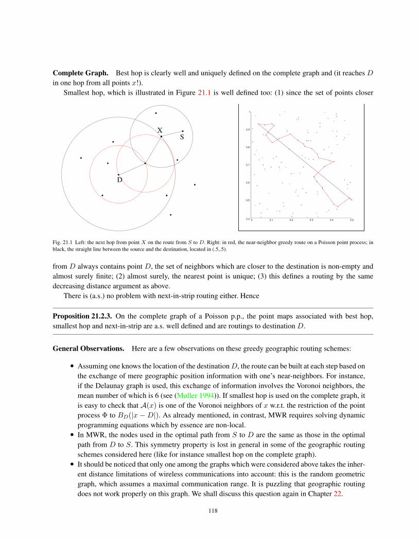
Complete Graph. Best hop is clearly well and uniquely defined on the complete graph and (it reaches Din one hop from all points x!).

Smallest hop, which is illustrated in Figure 21.1 is well defined too: (1) since the set of points closer

D

S

X

0.4

0.5

0.6

0.7

0.8

0.9

1

0 0.1 0.2 0.3 0.4 0.5

Fig. 21.1 Left: the next hop from point X on the route from S to D. Right: in red, the near-neighbor greedy route on a Poisson point process; inblack, the straight line between the source and the destination, located in (.5,.5).

from D always contains point D, the set of neighbors which are closer to the destination is non-empty andalmost surely finite; (2) almost surely, the nearest point is unique; (3) this defines a routing by the samedecreasing distance argument as above.

There is (a.s.) no problem with next-in-strip routing either. Hence

Proposition 21.2.3. On the complete graph of a Poisson p.p., the point maps associated with best hop,smallest hop and next-in-strip are a.s. well defined and are routings to destination D.

General Observations. Here are a few observations on these greedy geographic routing schemes:

• Assuming one knows the location of the destinationD, the route can be built at each step based onthe exchange of mere geographic position information with one’s near-neighbors. For instance,if the Delaunay graph is used, this exchange of information involves the Voronoi neighbors, themean number of which is 6 (see (Møller 1994)). If smallest hop is used on the complete graph, itis easy to check that A(x) is one of the Voronoi neighbors of x w.r.t. the restriction of the pointprocess Φ to BD(|x −D|). As already mentioned, in contrast, MWR requires solving dynamicprogramming equations which by essence are non-local.• In MWR, the nodes used in the optimal path from S to D are the same as those in the optimal

path from D to S. This symmetry property is lost in general in some of the geographic routingschemes considered here (like for instance smallest hop on the complete graph).• It should be noticed that only one among the graphs which were considered above takes the inher-

ent distance limitations of wireless communications into account: this is the random geometricgraph, which assumes a maximal communication range. It is puzzling that geographic routingdoes not work properly on this graph. We shall discuss this question again in Chapter 22.

118

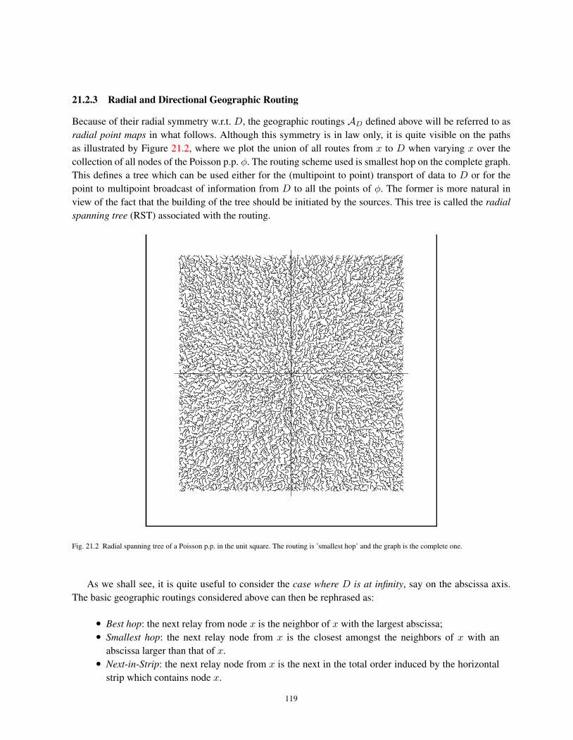
21.2.3 Radial and Directional Geographic Routing

Because of their radial symmetry w.r.t. D, the geographic routings AD defined above will be referred to asradial point maps in what follows. Although this symmetry is in law only, it is quite visible on the pathsas illustrated by Figure 21.2, where we plot the union of all routes from x to D when varying x over thecollection of all nodes of the Poisson p.p. φ. The routing scheme used is smallest hop on the complete graph.This defines a tree which can be used either for the (multipoint to point) transport of data to D or for thepoint to multipoint broadcast of information from D to all the points of φ. The former is more natural inview of the fact that the building of the tree should be initiated by the sources. This tree is called the radialspanning tree (RST) associated with the routing.

–

–

– –

Fig. 21.2 Radial spanning tree of a Poisson p.p. in the unit square. The routing is ’smallest hop’ and the graph is the complete one.

As we shall see, it is quite useful to consider the case where D is at infinity, say on the abscissa axis.The basic geographic routings considered above can then be rephrased as:

• Best hop: the next relay from node x is the neighbor of x with the largest abscissa;• Smallest hop: the next relay node from x is the closest amongst the neighbors of x with an

abscissa larger than that of x.• Next-in-Strip: the next relay node from x is the next in the total order induced by the horizontal

strip which contains node x.

119

These point maps will be referred to as directional point maps and is denoted byAd when the direction is d.The point is that the directional routes in general well approximate the radial ones on large S-D distances,except at the neighborhood of D.

The collection of all directional paths will be referred to as the directional spanning forest (DSF) associ-ated with the routing scheme.

Remark: The question whether the DSF of a Poisson p.p. on the whole plane is an infinite tree is open forall the cases mentioned above.

This chapter primarily focuses on two instances of routing on an homogeneous Poisson point process:next-in-strip and smallest hop. We consider both point to point and multicast schemes and both the radialand the directional cases.

21.3 Next-in-Strip Routing

We consider here next-in-strip routing on the complete graph. We focus on the directional case assumingthat the destination node is located at + infinity along the x direction.

Spatial Averages. From each relay node X , the progress P (X) is an exponential random variable withparameter λa, where λ is the intensity of the Poisson p.p. and a is the width of the strip. Using the fact thatthe absolute value of the difference between two independent uniform random variables on [−a/2, a/2] hasa density at u equal to 2u

a2 for 0 ≤ u ≤ a and equal to 0 elsewhere, we get that the length L(X) of the edgeto the next hop has for Laplace transform

LL(s) =∫r>0

∫0≤u≤a

exp(−s√r2 + u2)

2ua2λa exp(−λar)dudr

and for mean valueE0(L) =

∫r>0

∫0≤u≤a

√r2 + u2

2ua2λa exp(−λar)dudr ,

with L = L(0).

Route Averages. The progress sequence is i.i.d. so that the route average progress coincides with thespatial average progress and is equal to 1/(λa).

Let Xi = (xi, yi). The sequence {yi} is i.i.d. and each yi is uniform on (−a/2, a/2]. The sequence{yi+1 − yi, xi+1 − xi} is stationary and ergodic. Let

li =√

(yi+1 − yi)2 + (xi+1 − xi)2 .

Due to the pointwise ergodic theorem, the route average of the hop lengths 1n

∑ni=0 li converges a.s. to

the spatial mean E0(L) (evaluated above) when n tends to infinity. One can also evaluate the geometricinefficiency of the algorithm defined as

limn→∞

1n

n∑i=0

|yi+1 − yi|

by the same argument.We now give a result generalizing the above observations.

120

Lemma 21.3.1. The projection of the points of the strip on the x axis forms a Poisson p.p. Ψ = {Ti} on theline with intensity λa. Let Φi = STiΦ (resp. Φi = SXiΦ), i ∈ Z, be the node point process Φ translated insuch a way that point Ti (resp. Xi) stands at the origin — see Chapter 10 in Volume I for these definitions.For all functions g : M→ R+,

limn→∞

1n

n∑i=1

g(Φi) = E[g(Φ + δV )] (21.1)

P a.s. where V = (0, U) with U uniform on [−a/2, a/2] and independent of Φ. In addition

limn→∞

1n

n∑i=1

g(Φi) = E0Φ[g(Φ)] (21.2)

P a.s.

Proof. Since {Φi} (resp. {Φi}) is a sequence of marks of Ψ, it follows that Ψ = {Ti, Φi} (resp. Ψ ={Ti,Φi}) is a stationary and ergodic marked point process. The stationarity and the ergodicity are inheritedfrom the fact that the translation operator in the x direction is P-invariant and ergodic. Hence, by the ergodictheorem, for all functions g : M→ R+,

limn→∞

1n

n∑i=1

g(Φi) = E0Ψ[g(Φ0)], (resp. lim

n→∞

1n

n∑i=1

g(Φi) = E0Ψ[g(Φ0)])

P a.s. where P0Ψ is the Palm distribution w.r.t. Ψ. This shows the convergence of route averages. But by

Slivnyak’s theorem,

E0Ψ[g(Φ0)] = E[g(Φ + δV )]

and

E0Ψ[g(Φ0)] = E[g(Φ + δ0)] = E0

Φ[g(Φ)].

21.4 Smallest Hop Routing — Spatial Averages

This section focuses on smallest hop routing on the complete graph of a Poisson p.p.

21.4.1 Edge Length and Progress in Radial Routes

Throughout this section, X is a point of R2 and PO,X is the Palm probability of the Poisson p.p. Φ at(O,X), namely the law of a stationary Poisson p.p. with two additional points, one at the origin O and oneat X . Without loss of generality, we assume that the destination is D = O.

Scale Invariance. Since the route is scale-invariant, without loss of generality, we can set λ = 1; for ageneral λ, all results follow by multiplying distances by

√λ.

121

Edge Length. Let X ∈ R2 and L(X) = |X −A(X)|. For all r ≥ 0,

PO,X(L(X) ≥ r) = 1(r ≤ |X|)P(Φ(B◦X(r) ∩B◦O(|X|)) = 0) = 1(r ≤ |X|)e−M(|X|,r), (21.3)

where M(x, r) is the surface of the lens of the right part of Figure 21.3. Using the formula for the surfacedepicted by the left part of Figure 21.3, we get that :

M(x, r) = x2

(φ− sin(2φ)

2

)+ r2

(π

2− φ

2− sin(φ)

2

), (21.4)

with φ = 2 arcsin r2x . Notice that the distribution function of L(X), which only depends on |X|, is not

theta

����������������������0 T

P(X)

����������������������������������

r

Xpsi phi

0

y

��

Fig. 21.3 Left: the surface of this auxiliary dashed lens is equal to |T |2

2|2θ − sin 2θ|. Right: the dashed lens with surface M(x, r).

stochastically monotone in |X|. Its mean, which is plotted in Figure 21.4, is not monotone in |X| either.Given L(X) = r < |X|, consider the angle θ(X) of the edge from X to A(X). Using the property of

the right part of Figure 21.3 that ψ = π/2 − φ/2, we get that θ(X) is uniformly distributed on the interval(π + arg(X) − ψ, π + arg(X) + ψ), with cosψ = sin(φ/2) = r/(2|X|), that is ψ = arccos r

2|X| . GivenL(X) = |X|, the angle θ(X) is π + arg(X).

The joint distribution function of (L(X), θ(X)) is equal to

1(r ∈ (0, |X|)) ddrM(|X|, r)e−M(|X|,r)dr × 1(θ ∈ (π + arg(X)− ψ, π + arg(X) + ψ))

dθ2ψ

+δ|X|(dr)δπ+arg(X)(dθ)e−M(|X|,|X|). (21.5)

Progress. The progress from point X ∈ Φ is defined as P (X) = |X|− |A(X)|. It is equal to the length ofthe projection of the edge (X,A(X)) on the 0X line. The mean progress is plotted in function of |X| = x

in Figure 21.4.

21.4.2 Asymptotic Analysis

We now look at what happens when |X| tends to infinity. A direct computation gives:

lim|X|→+∞

PO,X(L(X) ≥ r) = exp(−πr2

2). (21.6)

122

In particular,

lim|X|→+∞

EO,X [L(X)] =

∞∫0

e−πr2

2 dr =1√2. (21.7)

By similar arguments, the asymptotic progress has for Laplace transform

lim|X|→+∞

EO,X(e−sP (X)) =1π

∞∫r=0

π/2∫θ=−π/2

e−sr cos θ exp(−πr2

2)πrdrdθ

=

∞∫r=0

π/2∫θ=−π/2

e−sr cos θ exp(−πr2

2)rdrdθ. (21.8)

In particular, the mean asymptotic progress is

lim|X|→+∞

EO,X(P (X)) =1π

∞∫r=0

π/2∫θ=−π/2

exp(−πr2

2) cos θdrdθ =

√2π. (21.9)

0.1

0.2

0.3

0.4

0.5

0.6

0.7

2 4 6 8 10

x

0

0.1

0.2

0.3

0.4

0.5

0.6

2 4 6 8 10

x

Fig. 21.4 Left: Mean of L(X) in function of x. Right: Mean of P (X) in function of x = |X|.

21.5 Smallest Hop Multicast Routing — Spatial Averages

This section is focused on the RST associated with smallest hop routing. In what follows, we study thedegree of nodes in the RST T associated with a Poisson p.p. Φ of intensity 1 which is considered under itsPalm version at O (the root is the origin of the plane).

• when the tree is used for multicasting, the degree determines the number of times a given symbolreceived by the node should be forwarded to the offspring nodes;• when the tree is used for the gathering of information at the root (see Remark 25.3.3), the degree

determines the number of links converging to the node.

123

21.5.1 Degree of Nodes

The degree of the source node O is

D(O) =∑

xi∈Φ\O

1(Φ(B◦xi(|xi|) ∩B◦O(|xi|)) = 0).

Hence, using Campbell’s formula, we get

EOD(O) = 2π

∞∫0

e−r2(2π/3−sin(2π/3)rdr =

π

2π/3−√

3/2∼ 2.56. (21.10)

Lemma 21.5.1. The degree of node O is bounded from above by 5 a.s.

Proof. Order the points directly attached to the origin by increasing polar angle. Let X and Y denote twoneighboring points in this sequence. Assume | ~OX| < | ~OY |. Denote by φ the angle between these twovectors. We have

| ~XY |2 = | ~OX|2 + | ~OY |2 − 2| ~OX|| ~OY | cosφ.

Since Y is attached to the origin, necessarily | ~XY |2 > | ~OY |2, which implies that

2| ~OX|| ~OY | cosφ < | ~OX|2.

Using now the assumption that | ~OX| < | ~OY |, we get cosφ < 1/2. Hence |φ| > π/3.

The degree of node X 6= O is given by :

D(X) = 1 +∑xi∈Φ

1(|xi| ≥ |X|)1(Φ(B◦xi(|X − xi|) ∩B◦O(|xi|)) = 0)1(O /∈ B◦xi(|X − xi|)).(21.11)

Indeed, a point x of norm larger than |X| shares an edge with X if and only if there is no point of smallernorm closer from x than X .

Let X 6= 0 and |X| = r. Obviously, E0,XD(X) depends on r only and with an abuse of notation, weoften write ED(r) in place of E0,XD(X). Taking the expectation of Equation (21.11) w.r.t PO,X , using thefact that the p.p. outside the ball of radius r is Poisson and making use of Campbell’s formula, we get

ED(r) = 1 + E∑xi∈Φ

1(Φ(B◦xi(|X − xi|) ∩B◦O(|xi|)) = 0)1(r ≤ |xi|)1(|xi| > |X − xi|)

= 1 +∫ρ>r

arccos( r2ρ

)∫− arccos( r

2ρ)

e−Q(r,ρ,θ)ρdρdθ,

where Q(r, ρ, θ) is the dashed surface in Figure 21.5 for X = (r, 0) and x = (ρ, θ). The condition that|x| > |X − x| (or equivalently that θ belongs to the interval (− arccos( r

2ρ), arccos( r2ρ)) translates the fact

that the origin should not be contained in this lens. Hence

ED(r) = 1 +∫ρ>r

arccos( r2ρ

)∫− arccos( r

2ρ)

e−ρ2

2|2α−sin 2α|e−

ρ2+r2−2ρx cos θ2

|2β−sin 2β|ρdρdθ,

124

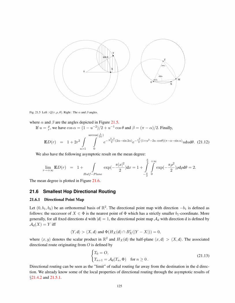
Q(X,T)

��

��

������������������0

X

T

T

��

��

����

��

������������������

theta

alpha

beta

0X

M

Fig. 21.5 Left : Q(r, ρ, θ). Right : The α and β angles.

where α and β are the angles depicted in Figure 21.5.If u = ρ

r , we have cosα = (1− u−2)/2 + u−1 cos θ and β = (π − α)/2. Finally,

ED(r) = 1 + 2r2

∫u>1

arccos( 12u

)∫0

e−u2r2

2(2α−sin 2α)e−

r2

2(1+u2−2u cosθ)(π−α−sinα)ududθ. (21.12)

We also have the following asymptotic result on the mean degree:

limr→+∞

ED(r) = 1 +∫

Half−Plane

exp(−π|x|2

2)dx = 1 +

π2∫

−π2

+∞∫0

exp(−πρ2

2)ρdρdθ = 2.

The mean degree is plotted in Figure 21.6.

21.6 Smallest Hop Directional Routing

21.6.1 Directional Point Map

Let (0, b1, b2) be an orthonormal basis of R2. The directional point map with direction −b1 is defined asfollows: the successor of X ∈ Φ is the nearest point of Φ which has a strictly smaller b1-coordinate. Moregenerally, for all fixed directions d with |d| = 1, the directional point map Ad with direction d is defined byAd(X) = Y iff

〈Y, d〉 > 〈X, d〉 and Φ(HX(d) ∩B◦X(|Y −X|)) = 0,

where 〈x, y〉 denotes the scalar product in R2 and HX(d) the half-plane 〈x, d〉 > 〈X, d〉. The associateddirectional route originating from O is defined by{

T0 = O,

Tn+1 = Ad(Tn,Φ) for n ≥ 0 .(21.13)

Directional routing can be seen as the ”limit” of radial routing far away from the destination in the d direc-tion. We already know some of the local properties of directional routing through the asymptotic results of§21.4.2 and 21.5.1.

125

2.1

2.2

2.3

2.4

2 4 6 8 10y

Fig. 21.6 ED(r) as function of r > 0.

21.6.2 Directed Spanning Forest

We define the Directed Spanning Forest (DSF) Td as the union of all the directional routes stemming fromall the points of Φ.

The following lemma, on the support of the degree of the DSF, is surprising in view of Lemma 21.5.1.

Lemma 21.6.1. The degree of a node of the DSF is not bounded and in the RST, a.s.

supx∈Φ

D(x) = +∞.

Proof. Without loss of generality we take d = −b1. The DSF built on the point set {Xn = (2−n, 3n), n ∈N} ∪ {O} gives: for all n, Ad(Xn) = 0, in particular the degree of the origin is infinite.

We now prove prove the second statement of the lemma.Let M ∈ N∗; for n ≥ 0, we define Un = [2−n − ε, 2−n + ε]× [3n − ε, 3n + ε], U−1 = [−ε, ε]× [−ε, ε],

AM = BO(4M )\(∪−1≤n≤M Un

)and

EM (X) = {Φ(X +AM ) = 0,Φ(X + Un) = 1,−1 ≤ n ≤M}.

We have P(EM (X)) = δ > 0 and if |X − Y | > 2.4M , EM (X) and EM (Y ) are independent (for ε smallenough).

For ε small enough, if EM (X) occurs, the point in U−1(X) has degree at least M in Td. Similarly forthe RST, if |X| is large enough and if EM (X) occurs, the point in U−1(X) has degree at least M in T .

Using the independence of the eventsEM (2k4Mb1), k ∈ N, we deduce that these events appear infinitelyoften.

126

21.7 Space and Route Averages of Smallest Hop Routing

21.7.1 Spatial Averages

The mean values computed in the previous sections are in fact spatial averages. We illustrate this statementon the edge length case.

Consider the RST with root 0 under PO. Let Lr be the sum of the edge length over all points includedin the ball B0(r), namely:

Lr =∑X∈Φ

1(X ∈ B0(r))|X −A(X)| =∑

X∈Φ\{O}

1(X ∈ B0(r))|X −A(X)|. (21.14)

From Campbell’s formula

EOLr =∫

BO(r)

EO,x(L(x))dx = 2π

r∫0

E(0,0),(0,t)(L((0, t)))tdt .

The change of variable u = tr gives

EOLrr2

= 2π

1∫0

uE(0,0),(0,ru)L((0, ru))du.

The dominated convergence theorem together with Equation (21.7) gives

limr→∞

EOLrr2

= 2π

1∫0

u1√2

du = π/√

2. (21.15)

The following stronger result is proved in (Baccelli and Bordenave 2007) using concentration inequalities:

Lemma 21.7.1. Almost surely and in L1,

limr→∞

Lrπr2

= lim|X|→+∞

EO,X [L(X)] =1√2. (21.16)

This extends to other quantities of the form g(A(X) −X), where g is some function from R2 to R, whichallows one to consider e.g. progress.

21.7.2 Route Averages

21.7.2.1 Existence

Two natural questions arise in connection with the definition of e.g. the directional greedy route in (21.13).For all g as above, let

Sn =1n

n∑k=1

g(Tk−1 − Tk), (21.17)

be the empirical route averages associated with g. Here are the two main questions related with this:

(1) Does Sn a.s. converge to some limit when n tends to infinity?(2) If so, does this limit coincide with the corresponding spatial average?

The answer to the first question is positive:

127

Theorem 21.7.2. There exists a unique probability measure π on R2 such that for all measurable functionsg such that g(X) ≤ max(C, |X|α) for some C > 0 and α > 0,

limn→∞

Snn

=∫R2

g(x)π(dx) = π(g). (21.18)

This theorem, which is proved in (Baccelli and Bordenave 2007), leverages the fact that certain sub-sequences of the sequence of segments that constitute a directional route form a Markov chain with a non-discrete state space. This chain is a Harris chain. It admits a small set and it is geometrically ergodic (Meynand Tweedie 1993). This result allows one to characterizes the asymptotic behavior of directional routes:

Corollary 21.7.3. There exists positive constants p and py such that

limn→∞

1n

n−1∑k=0

〈Tk − Tk+1, b1〉 = px = p, (21.19)

limn→∞

1n

n−1∑k=0

|〈Tk − Tk+1, b2〉| = py , (21.20)

where p is the route average of the directional progress and py that of the typical inefficiency; for all α > 0,there exists a constant lα such that

limn→∞

1n

n−1∑k=0

|Tk+1 − Tk|α = lα. (21.21)

21.7.2.2 The Routing Paradox and the Price of Anarchy in Routing

The answer to the second question is negative (in contrast with what happens in the strip routing case): bysimulation of 20000 transitions of the chain, one obtains that p ≈ .504, py ≈ .46 and l1 ≈ .75. The valueof p is significantly larger than the spatial average of the mean asymptotic progress as evaluated in (21.9),which is approx. equal to 0.450. A similar observation holds for l1 when compared to (21.6): as it is the casefor progress, the mean magnitude of the hop from a point to its successor (l1 ≈ .75) is ”boosted” by the factthat one is located on a long route, compared to the spatial average value (which is appr. equal to .71). Theanalysis of the Markov chain alluded to above allows one to understand why this happens.

It can in addition be proved that route averages over long radial paths coincide with route averages onlong directional routes (see (Baccelli and Bordenave 2007) for a proof). Hence, one can rephrase the resultsof the last corollary as follows: consider the greedy route from a source to a destination at distance t fromone another; then for a p.p. Φ with intensity λ,

• The mean number of hops on the greedy route scales like 1.98t/√λ (since this mean number of

hops is approximately equal to t/0.504 for large t when λ = 1);• The greedy route κ-approximates Euclidean distance with κ ≈ 1.48 (since the mean length of

the route is approximately equal to t ∗ 0.75/0.504 for large t when λ = 1).

128

Comparing these results to the corresponding ones on optimal routes on the Poisson–Delaunay graph (see§ 20.3.2), we can say that the price of anarchy which we define as the ratio of the greedy cost and of theoptimal cost is 1.48/1.05 ≈ 1.41 in terms of Euclidean distance.

21.7.2.3 Maximal Deviation

We end this section with a result on the deviation of the path from its mean, also proved in (Baccelli andBordenave 2007). Let R(x) or R(X) denote the path from X = (x, 0) in the DSF with direction −b1; R(x)may be parameterized as a piecewise linear curve (t, Y (t))t≤x in R2. The maximal deviation of this curvebetween x′ and x with x′ ≤ x is defined as

∆(x, x′) = supt∈[x′,x]

|Y (t)|. (21.22)

Theorem 21.7.4. For all x ≥ x′, for all ε > 0 and all integers n,

P(∆(x, x′) ≥ |x− x′|12

+ε) = O(|x− x′|−n).

21.8 Radial Spanning Tree in a Voronoi Cell

In this section, we extend the RST to situations where there is a collection of trees (a forest) rather than asingle one. We use the context of sensor networks (see Remark 25.3.3) to describe the construction. Considertwo independent Poisson p.p.: Φ0 = {x0

n}, the p.p. of cluster heads, of intensity λ0 and Φ1 = {x1n}, the p.p.

of sensor nodes, with intensity λ1. The first p.p. tessellates the plane in Voronoi cells. We denote by Vn theVoronoi cell of point x0

n w.r.t. the points of Φ0. Two forests can then be defined in relation with this VT:

• The family of internal RSTs: the n-th tree of this forest, Tn, is the RST built using the points ofΦ1 that are contained in Vn, with x0

n as a root.• The family of local RSTs: if node X belongs to Vn, one defines its successor as the point of

(Φ1 ∪ {x0n}) ∩ B◦x0

n(|X − x0

n|) that is the closest to X . Notice that this successor does notnecessarily belong to Vn. Nevertheless, this rule defines a forest too (see Lemma 21.8.1). Onethen defines the n-th local RST tree Un as the tree which is the union of all the routes from sensornodes with ultimate successor x0

n.

In what follows, we concentrate on the second case which can be analyzed using the same type of tools asin §21.5. Figure 21.7 depicts a sample of such a forest.

Lemma 21.8.1. Almost surely, there exists no node X of Φ0 such that the sequence of successors of Xbased on the local RST rule contains node X .

Proof. Let {Yi}i≥0 be the sequence of successors of X = Y0. If Yi = X for some i > 0, then necessarilythe points of {Yi} belong to different Voronoi cells (if this were not the case, then the distance to the clusterhead of the cell to which all points belong would be strictly decreasing, which forbids cycles). Then one canrewrite {Yi}i≥0 as

{Yi}i≥0 = {Z0(1), . . . , Z0(n0), Z1(1), . . . , Z1(n1), . . . , Zj(1), . . . , Zj(k), ...}

129

0

0.2

0.4

0.6

0.8

1

0.2 0.4 0.6 0.8 1

Fig. 21.7 Local Voronoi radial spanning trees (in blue) of 600 sensor nodes uniformly and independently distributed in the unit square, w.r.t 10cluster heads (in red), also uniformly and independently distributed in the unit square. The Voronoi cell of one of the cluster heads is depicted inred.

with Zl(1), . . . , Zl(nl) ∈Wl for all 0 ≤ l ≤ j, where {Wj}j≥0 is a sequence of cells such that Wl 6= Wl+1

for all l < j, nl is a sequence of integers and Zj(k) = X . Let Sl denote the cluster head of Wl. Then thedefinition of the local RST implies that a.s.

|X − S0| = |Z0(1)− S0| > |Z0(2)− S0| > · · · > |Z0(n0)− S0| > |Z1(1)− S0|.

Since Z1(1) belongs to W1, we have a.s.

|Z1(1)− S0| > |Z1(1)− S1|.

For the same reasons, for all l = 1, . . . , j − 1

|Zl(1)− Sl| > |Zl(2)− Sl| > · · · > |Zl(nl)− Sl| > |Zl+1(1)− Sl|

and

|Zl+1(1)− Sl| > |Zl+1(1)− Sl+1|, a.s.

130

In addition

|Zj(1)− Sj | > |Zl(2)− Sl| > · · · > |Zj(k)− Sj | = |X − S0|.

Hence a contradiction.

Let Ln denote the total length of all edges from nodes in Vn. Let E0 denote the Palm probability w.r.t.Φ0. We have

Ln =∑m

1(x1m ∈ Vn)Lm,

where Lm is the length of the link that connects x1m to its successor. Using the fact that x1

m ∈ Vn iffΦ0(B◦x1

m(|x1

m−x0n|)) = 0 and the fact that Lm > uwith u < |x1

m−x0n| iff Φ1(B◦x1

m(u)∩B◦x0

n(|x1

m−x0n|)) =

0, we get from Campbell’s formula that

E0

(∑m

1(x1m ∈ Vn)Lm

)= 2πλ1

∞∫r=0

e−λ0πr2

r∫u=0

e−λ1M(r,u)du

rdr,

with M(r, u) the surface of the lens defined in §21.4. Hence

E0 (L0) = 2πλ1

∞∫r=0

e−λ0πr2

r∫u=0

e−λ1M(r,u)du

rdr. (21.23)

21.9 Conclusion

There are several interesting problems in relation with the topics considered in the present chapter. The firstline of thought concerns the extension of the analysis conducted for ”smallest hop closer to destination” toother natural routing schemes.

A second and more general question concerns the classification of greedy routing schemes according tothe following criteria:

• Price of anarchy: how much does the greedy path lose (e.g. in terms of Euclidean length or interms of number of hops) compared to the optimal path(s)?• Comparison of spatial and route averages: given that the latter are more difficult to evaluate than

the former, it would be interesting to learn whether there are general comparison rules betweenthe two. For instance, for strip routing the two types of averages coincide, whereas for ”smallesthop closer to destination”, they differ. Does there exist a general criterion for deciding whethera given routing scheme is of the first kind (with both averages coinciding) or of the second? In”smallest hop closer to destination”, route averages are ”better” than spatial averages (e.g. interms of progress). Can one identify the class of greedy schemes for which this property holdstrue?

In Chapter 20 and in the present chapter, the physical constraints of wireless links were essentiallyignored. Consider for instance ”smallest hop closer to destination”, which was argued to be the most sensiblerepresentation of routing in a wireless network within the context considered in the present chapter. Thedistance from a node to the next hop node may still be arbitrarily large as we saw; in addition the latter nodemay be surrounded by interferers which would result in a very small probability to have a good SINR on theconsidered link. This example shows that the routing principles considered so far should be revisited withinthe SINR geometry framework, which is the object of the next chapter.

131

22Time-Space Routing

22.1 Introduction

In Chapters 20 and 21, MAC and detection were ignored as already mentioned. But in addition time wasabsent (we considered routes on a snapshot as already mentioned) and when throughput was considered, itwas in terms of a Shannon like formula.

In contrast, the time–space multihop routing schemes considered in this chapter take MAC decisions andfading variables into account as well as their variability w.r.t. time. The setting is again a Poisson MANETwith a MAC of the Aloha type. The packet communication model is used, with a definition for the captureof packets which is based on the SINR model of § 16.2.

Here is a first basic dichotomy for the routing schemes to be considered in this chapter. We distinguishbetween:

• Layer-aware routing schemes, where the route between S and D is defined once and for all (e.g.through a static point map as considered in the last two chapters) and where the MAC is thenasked to realize this route coping with the time and space variations of fading;• Cross-layer routing schemes, where there is no predefined route and where the routing scheme

tries to take advantage of the variability of MAC and fading to decide on the next relay for eachpacket at each time slot.

Section 22.2 describes the stochastic setting allowing us to define time–space routing. Section 22.3focuses on the key notions pertaining to this type of routing. In particular, we introduce a new random graphthat we call the time–space SINR graph and the notion of time–space point map. We also define the notionsof route averages associated with these maps.

The other sections of the chapter focus on instances of such time–space routing algorithms. Sec-tion 22.4.2 bears on the layer-aware case whereas all other sections bear on the cross-layer case. Section 22.5is concerned with minimal weight time–space routes. These optimal routes have no practical meaning astheir determination would require full knowledge of the future fading and MAC variables of all nodes.However, their mathematical properties shed light on many other algorithms and in particular on greedy

133

time–space routes. They also provide intrinsic performance limitations on this class of schemes. Greedytime–space routing (called opportunistic routing below) is studied in § 22.6. Let us stress that opportunisticrouting is based on the inherent multicast nature of Spatial Aloha and not on Opportunistic Aloha as definedin Chapter 16.

In terms of performance evaluation, the chapter contains several open questions and a few negativeresults, like e.g. the fact that in several cases, either the mean end-to-end delay of a packet scales super-linearly with the distance between source and destination, or the asymptotic velocity of a typical packet is0, even if this packet is considered as a priority packet and experiences no queuing in the nodes. Among thepositive results, let us quote the optimal tuning of the MAC parameters and the proof of scaling laws. Anotherpractical conclusion of this chapter is that for source-destination pairs at finite distance, opportunistic routingvery significantly outperforms layer-aware routing schemes. This holds true even when the latter use optimalstatic routing algorithms as considered in § 20.2.

22.2 Stochastic Model

We adopt the MANET receiver model introduced in § 17.5, which is briefly recalled below.

22.2.1 MANET Model

In this model the nodes can be represented by an i.m. p.p.. with cross fading (cf. Section 2.3.3.2 in Volume I)and node dependent noise. More precisely we consider the space-time scenario of Section 17.5.1 (see alsoSection 17.5.6), described by Φ = {(Xi, ei(n),Fi(n),Wi(n))}, where:

(1rout) Φ = {Xi} denotes the locations of the MANET nodes. Two options are considered in whatfollows:

– Poisson MANET, where Φ is a Poisson p.p. with intensity λ. This is our default optiondenoted by GI

W+M / GI .

– Poisson MANET Model with an Additional Periodic Infrastructure: we also considernetworks with an additional periodic infrastructure, denoted by GI

W+(M+Gs) / GI in whichΦ = ΦM+ΦGs ; here ΦM is some homogeneous Poisson p.p. with intensity λM and ΦGs

is a stationary p.p. of periodic nodes. The points of ΦGs are assumed to be located on asquare grid Gs with edge length s. See Example 4.2.5 in Volume I on how to constructsuch a stationary periodic structure. We assume that ΦM and ΦGs are independent. Theintensity of ΦGs is 1/s2 and that of Φ is λ = λM + 1/s2. The MAC and the multi-hoprouting mechanisms take place on all the nodes of Φ.

(2rout) ei(n) = {ei(n) : n}i are the MAC indicators of the node i at time n; ei(n) are i.i.d. in i and nwith with P{ e(n) = 1 } = 1−P{ e(n) = 0 } = p.

(4rout) Fi = {F ji (n) : j, n}i are the virtual powers (comprising fading effects) emitted by node i tonodes j at time n. We consider the following scenarios for the time dependence between thefading variables:

– No fading case: F ji (n) ≡ µ−1 for all i, j, n;

– Slow fading case: F ji (n) = F ji (0) for all i, j, n and F ji are i.i.d. as F with mean µ−1.This means that the fading is sampled independently for each transmitter–receiver pairand stay constant for all time slots.

134

– Fast fading case: F ji (n) are i.i.d. for all i, j, n, where F has mean µ−1.

Cf. Remark 17.5.1 on the fast/slow fading terminology.(5rout) Wi = {Wi(n) : n}i is a sequence of i.i.d. (in i and n) non-negative random variables represent-

ing the thermal noise at node i and at time n. This scenario, already considered in Section 17.5.6was called there receiver dependent, fast noise case.

For all points X,Y ∈ R2, let ΦX,Y = Φ ∪ {X,Y }. Let eX and eY be two independent MAC indicatorsequences distributed like e, that one attributes to nodes X and Y respectively, with similar definitions forFX and FY . By arguments similar to those of § 18.4.1, in the Poisson MANET case, the marked p.p. ΦX,Y

is also the Palm version of Φ w.r.t. the two points {X,Y }. We denote the corresponding Palm probabilityand expectation by PX,Y ,EX,Y respectively (i.e., Φ under PX,Y has the same distribution as ΦX,Y underP.)

22.2.2 SINR coverage

We assume that all the nodes are perfectly synchronized and at (discrete) time n the p.p. of transmittersis denoted by Φ1(n) =

∑i δXi1(ei(n) = 1). The interference at the node Xj with respect to the signal

emitted by the node Xi at time n (i.e., the power of the sum of all signals received at Xj at time n exceptthis emitted by Xi) denoted by I1

ij(n), can be represented as the shot-noise variable

I1ij(n) = IΦ1(n)\{Xi} =

∑Xk∈Φ1(n), k 6=i,j

F jk (n)/l(|Xj −Xk|).

Denote by δ(Xi, Xj , n) the indicator that the node Xi covers the node Xj at time n with the SINR atleast T , provided Xi is emitter Xi ∈ Φ1(n) and Xj is potential receiver Xj ∈ Φ0(n) = Φ \ Φ1(n) at timen. Formally δ(Xi, Xj , n) is the indicator that the condition (17.10) holds with F , I considered at time n andW = Wj(n).

22.3 The Time–Space Signal-to-Interference Ratio Graph and its Paths

In this section we will introduce an SINR graph with space-time vertexes. In this framework, as in the SINRgraph of Chapter 8 in Volume I, the random point process on the plane describes the locations of the users ofan ad-hoc network, however we consider also the discrete time dimension, which corresponds to successivetime slots in which these nodes exchange information (here packets). As we will see the study of this newmodel is motivated by multihop routing protocols. In this extended setting, a directed edge represents thefeasibility of the wireless transmission between two given network nodes at a given time.

22.3.1 Definition

Consider a general stationary MANET model Φ as above.Define the set of SINR-neighbors of Xi ∈ Φ at time n as the set of receivers which successfully capture

the packet transmitted by Xi at time n if Xi transmits at that time, and as {Xi} otherwise:

V (Xi, n) =

{{Xi} ∪ {Xj : Xj ∈ Φ0(n) s.t. δ(Xi, Xj , n) = 1} ifXi ∈ Φ1(n)

{Xi} otherwise.(22.1)

135

����

����

����

����

����

����

����

����

����

����

����

����

����

X X Xi+1 j

n+1

n

m

i

Fig. 22.1 The directed graph GSINR on Φ × Z, where Φ is a p.p. on the real line. The transmitters are depicted by black dots and the potentialreceivers by white ones.

The time–space SINR graph GSINR is a directed graph on Φ×Z defined as follows: the nodes of GSINR areall the pairs of the form (Xi, n) with Xi ∈ Φ and n ∈ Z; all edges are of the form ((Xi, n), (Xj , n + 1));there is an edge from (Xi, n) to (Xj , n + 1) if Xj ∈ V (Xi, n) (see Figure 22.1 which gives an illustrationof this graph in the case of a 1D MANET).

Let us stress an important convention in our terminology. By network node, or point, we understand apoint of Φ. A (graph) vertex is an element of Φ× Z; i.e. it represents some network node at some time. Theexistence of a graph edge is to be interpreted as the possibility of a successful communication between twonetwork nodes (those involved in the edge) at time n. This can be rephrased as follows. Suppose that at timen the network node Xi has a packet (containing some information). Then the set of graph neighbors of thevertex (Xi, n) describes all the nodes that can decode this packet at time n+ 1. Thus any path on the graphGSINR represents some possible route of the packet in space and time.

22.3.2 Time–Space Paths

Note first that GSINR has no isolated nodes in the usual sense. Indeed, we have always (Xi, n) connected to(Xi, n + 1). We will consider directed paths on GSINR and call them paths for short. Note that these pathsare self-avoiding due to the fact that there are no loops in the time dimension.

In view of what was said, a path of GSINR originating from node (S, k) and with q (time) steps is acollection of nodes

{(Zi, i)}i=k,...,k+q

such that Zi ∈ Φ for all i, Zk = S and Zi+1 ∈ V (Zi, i) (or equivalently, there is an edge from (Zi, i) to(Zi+1, i+ 1) in GSINR) for all i = k, . . . , q − 1.

The following general terminology is used in the context of such a path:

• its Euclidean length is∑q−1

i=0 |Zi+1 − Zi|;• its time length is its total number of time steps q;• its number of hops H is the number of different points of Φ visited by the path;• if Zi−1 6= X and Zi = X , its local delays at (X, i), denoted by L(X, i) is the smallest integerj > 0 such that Zi+j 6= X (see § 17.5).

136

Denote by Hout,ki (n) the number of paths of length k (i.e. with k edges) originating from (Xi, n).Similarly, denote by Hin,ki (n) the number of such path terminating at (Xi, n). In particular Houti (n) =Hout,1i (n) andHini (n) = Hin,1i (n) are respectively, the out- and in-degree of the node (Xi, n).

The following two results regarding the number of paths are obtained under a general p.p. and fadingassumptions.

Lemma 22.3.1. For a general p.p. Φ and a general fading model, the in-degreeHini of any node of GSINR isbounded from above by the constant ξ = 1/T + 2.

Proof. It follows immediately from the proof of Lemma 17.3.4.

Note also that under some additional assumptions one can take ξ = 1/T + 1 (cf Lemma 17.3.4.)Let

hout,k = E0[Hout,k0 (n)] = E0[Hout,k0 (0)]

andhin,k = E0[Hin,k0 (n)] = E0[Hin,k0 (0)]

be the expected numbers of paths of length k originating or terminating at the typical node, respectively. Inparticular hout = hout,1 and hin = hin,1 are the mean out- and in-degree of the typical node, respectively.

Lemma 22.3.2. For a general p.p. Φ and a general fading model

hin,k = hout,k . (22.2)

Proof. We use the mass transport principle to get that E0[Hout,k0 (0)] = E0[Hin,k0 (0)], which implies thedesired result. Indeed, Campbell’s formula and stationarity give

λhout,k = λ

∫[0,1)2

E0[Hout,k0 (0)]dx

= E[ ∑Xi∈Φ∩[0,1)2

Hout,ki (0)]

=∑v∈Z

E[ ∑Xi∈[0,1)2

∑Xj∈[0,1)2+v

# of paths from (Xi, 0) to (Xj , k)]

=∑v∈Z

E[ ∑Xi∈[0,1)2−v

∑Xj∈[0,1)2

# of paths from (Xi, 0) to (Xj , k)]

= λ

∫[0,1)2

E0[Hin,k0 (k)]dx = λhin,k ,

where # denotes the cardinality. This completes the proof.

Here are immediate consequences of the two above lemmas.

137

Corollary 22.3.3. Under the assumptions of Lemma 22.3.1:

• GSINR is locally finite (both on in- and out-degrees of all nodes are P-a.s. finite).• Hin,ki (n) ≤ ξk P-a.s for all i, n, k.• hin,k = hout,k ≤ ξk for all k.

Here is a graph theoretic summary of further results that one can prove on GSINR graph (see (Baccelli,Błaszczyszyn, and Mirsadeghi 2009) for the details). Some of these results will be revisited in the remainingpart of this chapter.

• This graph is a.s. connected in the sense that for all S and D in Φ and all k ∈ Z, there a.s. existsa path from (S, k) to the set {(D, k + l)}l∈N (cf. Corollary 22.4.4).• For the M

W+(M+Gs) / M fast fading case, if thermal noise is positive, then the first passage perco-lation delay rate is finite (Proposition 22.5.6) and has a positive mean (Proposition 22.5.5). Byfirst passage percolation, we mean here the path from (S, k) to the set {(D, k + l)}l∈N with thesmallest number of time steps N . By delay rate, we mean the limit when it exists of the ratioN/|S −D|, when |S −D| tends to infinity. In many first passage percolation models, the limitof this ratio is a constant and is then referred to as the time constant. As we shall see, this is notthe case here and this explains our terminology.• For the M

W+M / M fast fading case, if thermal noise is positive, then the mean value of the firstpassage percolation delay rate is infinite (cf. Proposition 22.5.9 for the precise statement).

22.4 Routing and Time–Space Point Maps

We now use the time–space SINR graph GSINR in the context of routing in ad-hoc networks. We have alreadyseen in previous chapters that in many cases the route followed by a packet can be naturally described bymeans of the iterations of some point map. We now extend this concept to the time–space scenario of GSINR.

22.4.1 Time–Space Point Maps

A time–space path is often defined from a time–space point map, that is a collection of point maps {An},where An(X) is an algorithm which selects the next hop for a packet located at X at time n in the setV (X,n). The path originating from node (S, k) is then defined by the recursion

Zi+1 = Ai(Zi), i = k, . . . , q − 1 , (22.3)

with initial condition Zk = S. This gives the route followed by a priority packet1 starting from node S ∈ Φat time k.

The fact that this algorithm builds a path of GSINR implies that two key phenomena are taken intoaccount: collisions (lack of capture by any node) and contention for channel (only time slots where the relaytosses heads are used for transmission); in particular, if there is no channel access for X at time k, thenV (X, k) = {X}.

1In the considered MANET, a node may have to relay packets of several flows, namely associated with several S-D pairs; packets located on agiven node may hence have to queue for accessing the shared channel. By priority packet, we mean a packet which is assumed to be scheduledaccording to a preemptive priority rule on each node and which hence never experiences such queuing.

138

22.4.1.1 Radial Point Maps

The following definition is adopted by analogy with our definition of Chapter 21:

Definition 22.4.1. A time–space point map {An} is a radial routing to D if Ai(D) = D, for all i, and if inaddition, for all (S, k), Zi = D, for all i ≥ k + ∆ and for some ∆ = ∆(S, k) ∈ N.

The following terminology is used in the context of such a radial routing:

• its progress at time i is Pi = |Zi−D|−|Zi+1−D|, which may be 0 in case of collision or denialof channel access;• its end-to-end delay ∆ = ∆(S, k) is the total number of time steps required for the priority

packet to go from (S, k) to D;• its number of hops H = H(S, k) is the number of different nodes on the path;• if X is a node of the path originating from (S, k) (which we assume to be self avoiding) the local

delay L(X) = L(X,S, k) at node X is the number of time steps spent by the path at node X .

The following relation holds between these quantities:

∆ =H−1∑i=1

L(Xi) ,

when denoting by S = X1, . . . , XH = D the sequence of (different) nodes of the time–space path.Notice that the path and the end-to-end delay from (S, k) toD and that from (S, k′) toD differ in general

as typical in time–space routing.

Definition 22.4.2. A radial time–space routing satisfies the ball property if the route from S to D is con-tained in the ball BD(|D − S|).

22.4.1.2 Directional Point Maps

We also consider the case where D is located at infinity in some direction d of the plane (cf. Section 21.2.3).A time–space point map which converges to D will then be called a d-directional routing. In line with ourprevious definitions, when D is located at infinity in direction d, for all functions g : R2 → R, the almostsure limit

limN→∞

1N

N−1∑n=0

g(Zn+k+1 − Zn+k) (22.4)

is called the (time–space) route average of g (provided the limit exists). There are other natural route averagestaken hop by hop rather than w.r.t. time, like for instance the route average of the local delay

l = limM→∞

1M

M−1∑m=0

Lm , (22.5)

where Lm is the local delay at the m-th hop of the route. If the last almost sure limit exists, then one caninterpret v = l−1 as the route average velocity (measured in number of hops per time step):

v = limM→∞

M∑M−1m=0 Lm

. (22.6)

The remaining sections investigate the properties of a few basic classes of time–space routing algorithms.

139

22.4.2 Layer-aware Time–Space Point Maps

The simplest time–space routing algorithms are those where routing and MAC are fully separated. Namely,at any time step, the next relay node for a packet located at node X is A(X), where A is some static pointmap on Φ = {Xi}. More precisely the time–space route is then defined by the following time–space pointmap:

Bn(X) =

{A(X) if A(X) ∈ V (X,n),

X otherwise.(22.7)

Note that given Φ, Bn(X) is a random variable with two possible outcomes: X andA(X); as long asA(X)is not an SINR-neighbor of X , the packet stays at X . The first time it is an SINR-neighbor of X , the packetjumps there.

A key property, which contrasts with our findings on the existence of dead ends in geographic routing(see § 21.2.2), is that, for all X and all A such that A(X) is at finite distance from X , all packets located atX make it to A(X) in finite time under natural assumptions:

Lemma 22.4.3. Assume that 0 < p < 1. Then, under either of the following assumptions:

(a) the law of F has an infinite support on R+ (i.e. P{F > s} > 0 for all s) and we have fast fading,(b) W ≡ 0,

the local time L(X,n) of a packet starting at time n in node X is a.s. finite for all n ∈ Z.

Remark: Note that the infinite support assumption holds for all fading models considered so far: Rayleigh,Rician, Nakagami, Lognormal, etc.

Proof. We show that for all X ∈ Φ and all n ∈ Z, the probability that A(X) /∈ V (X,n+ l) for all l ≥ 1 is0.

We consider first case (a). Denote by G the σ-algebra generated by Φ (without its marks). Using the fastfading assumption, we get that conditionally on G,

P [ L(X, 0) ≥ l | G ] =l−1∏i=0

P [A(X) /∈ V (X, i) | G ] =(P [A(X) /∈ V (X, 0) | G ]

)l,

so that it is enough to prove that P [A(X) /∈ V (X, 0) | G ] < 1 to conclude the proof. But we have

P [A(X) ∈ V (X, 0) | G ]=p(1− p)P

[F/l(|X −A(X)|)W + IΦ1\{X,A(X)}

≥ T | G, eX = 1, eA(X) = 0

],

where F is the fading from X to A(X) at time 0, eX (resp. eA(X)) is the MAC decision of X (resp. A(X))at time 0 and IΦ1\{X,A(X)} is the interference atA(X) at time 0. Since F and IΦ1\{X,A(X)} are independent,

P

[F/l(|X −A(X)|)W + IΦ1\{X,A(X)}

≥ T | G, eX = 1, eA(X) = 0

]

=∫

R+

∫R+

H (T (w + z)l(|X −A(X)|)) fA(X)(dz)g(dw) > 0 ,

140

whereH is the tail of the c.d.f. of F , fA(X) is the conditional law of IΦ1\{X,A(X)} given G, eX = 1, eA(X) =0 and g the law ofW . The last (strict) inequality follows from the fact that IΦ1\{X,A(X)} is a.s. finite (becausethe path-loss exponent β is larger than 2) and from the assumption made on the support of F (that it isinfinite). This concludes the proof in this case.

Consider now case (b). Let H denote the σ-algebra generated by Φ and the fading variables (under theslow fading case, these variables do not vary over time). Using the fact that the MAC decisions are i.i.d., weget that

P [ L(X, 0) > l |H, ] = P [A(X) /∈ V (X, 0) |H ]l ,

so that it is enough to prove that P [A(X) /∈ V (X, 0) |H ] < 1. But

P [A(X) ∈ V (X, 0) |H ]

= P

[F/l(|X −A(X)|)IΦ1\{X,A(X)}

≥ T, eX = 1, eA(X) = 0 | H

]

= p(1− p)P[IΦ1\{X,A(X)} ≤

F/l(|X −A(X)|)T

| H, eX = 1, eA(X) = 0]> 0 ,

where the last inequality follows from the fact that the H-conditional law of the Poisson SN processIΦ1\{X,A(X)} puts a positive mass on the interval [0, z] for all positive z.

The following corollary shows that these layer-aware mechanisms are time–space routings to D providedthe underlying static point map is a routing to D (see the introduction of Part V for the definition):

Corollary 22.4.4. Consider a static point map A which is a routing to D (resp. a d-directional routing). Let{Bn} be the associated layer-aware time–space point map (22.7). Under the assumptions of Lemma 22.4.3,{Bn} is a time–space routing to D (resp. a d-directional time–space routing).

Proof. Conditionally on Φ (or H), each local delay is a.s. finite at each node of the route. Hence for all S,all n ≥ 1 and all k ∈ Z, the number of time steps required by this time–space path to reach node An(S)(the n-th node of the static route) is a.s. finite. In particular the end-to-end delay to reach D is a.s. finite. Theproof of the d-directional case is similar.

When taking ’smallest hop to destination’ as static point map (see § 21.2.1) in the last corollary, we get thatthere exists a time–space point map which satisfies the ball property and which is a routing to D.

Here are a few comments on the differences between the static greedy geographic routing schemes con-sidered in Chapter 21 and the layer-aware time–space greedy routings considered here. We found out inChapter 21 that next-in-strip routing on the random geometric graph (which takes the range limitations ofwireless communication into account) does not work properly because of the dead end problem. Corol-lary 22.4.4 shows that the time–space version considered here works better, in that a packet makes it to anyfinite destination (or any finite distance node of the route) in finite time under assumptions (a) or (b) andhence does not suffer of the dead end problem.

Remark 22.4.5. From the proof of the Lemma 22.4.3, we deduce that

• In case (a), conditionally on G, for all X and n, L(X,n) is a geometric random variable with aparameter that depends on X but not on n.

141

• In case (b), the same holds true conditionally onH.

We conclude this section with the analysis of two special cases: directional strip routing and directionalsmallest hop routing. We show that in these two cases, under rather natural conditions, the route average ofthe velocity of a priority packet is 0 (in a sense to be described precisely below). One can rephrase this bysaying that these schemes do not work properly over large scale routes in most practical cases.

22.4.2.1 Directional Strip Routing

Take directional strip routing (see § 21.3) as static point map and consider the associated time–space routingalgorithm as defined by (22.7). We deduce from what precedes that under either (a) or (b), a packet initiallylocated at S reaches the n-th hop of the (static) route in finite time for all n.

Consider now the route average local delay of a prioritypacket in this time–space routing framework.Rather than defining it through (22.5), we define this quantity as

limn→∞

1n

n∑i=0

E[L(Xi) | G] ,

where G denotes the σ-algebra of the Poisson p.p. Φ (without its marks). This allows us to use Lemma 21.3.1by posing g(Φi) = E[L(Xi) | G] (see the definition of Φi in this lemma) which implies that P a.s.,

limn→∞

1n

n∑i=0

E[L(Xi) | G] = E0[L(0)] .

The immediate conclusion is that when E0[L(0)] =∞, then the route average local delay is infinite, so thatthis routing mechanism does not work properly on a more global scale.

Example 22.4.6. Consider the example of fast Rayleigh fading (which falls in the considered frameworkunder assumption (a) of Lemma 22.4.3). In most practical cases, we have E0[L(0)] =∞.

• In the noise limited case, if the thermal noise is bounded from below by a constant W , then, bythe same arguments as in Proposition 17.5.9 (cf. also the discussion in Section 17.5.9), we getthat

E0[L(0)] ≥ λa

p(1− p)

∫r≥0

exp(−λar) exp(µTWl(r))dr =∞,

for all OPL attenuation models considered in this monograph.• In the interference limited case, by the same arguments as in Section 17.5.4.2, when using the

fact that the interference at the receiver is larger than that created by Φ1 in the half plane on theright of the receiver, we get that in the OPL 3 case,

E0[L(0)] ≥ λa

p(1− p)

∫r≥0

exp(−λar) exp(λπp(1− p)

2β−1K(β)T

2β r2)

dr =∞,

for all values of p and T .

142

22.4.2.2 Smallest Hop Directional Routing

Take now for static point map ’smallest hop’ on the complete graph as defined in § 21.2. More precisely,consider the directional point map associated with some direction d. Under Assumption (a) of Lemma 22.4.3,conditionally on G, the local delay at each node of the path is a geometric random variable with a non-degenerate parameter so that the routing mechanism works locally.

The conditions under which the route average local delay is finite are unknown as to the publication ofthis monograph. The fact that the spatial average of the local delay E0[L] in a cone of angle π is infinite (seeRemark 17.5.14) does not immediately imply that l is infinite too. However, if E0[L] = ∞ and the almostsure limit (22.5) holds for some finite l, then the last limit cannot hold in L1.

22.5 Minimal End-to-End Delay Time–Space Paths

The aim of this section is to define optimal paths from S to D within this time–space setting. As alreadymentioned, these optimal paths, which can in principle be obtained by dynamic programming, are in factimpractical. In addition to requiring global knowledge, namely knowledge of what happens far away inspace, they also require the knowledge of future fading variables and MAC indicators. This explains ourfocus on greedy routing schemes in the forthcoming sections. Nevertheless, the scaling law establishedbelow on minimal weight paths is useful for the analysis of these greedy schemes in that it provides thefundamental limitations of all possible time–space schemes.

We focus here on paths with the smallest number of time steps. This is tantamount to finding minimalweight paths on GSINR when associating a weight w = 1 to each edge of this graph.

Consider the set C(k, i, j) of all self-avoiding paths of GSINR which start at time k from node Xi, reachXj at some time l > k and satisfy the ball property. It follows from Corollary 22.4.4 (or from Lemma 22.6.1below) that if either of the two conditions (a) and (b) of Lemma 22.4.3 holds, then for all i, j and k, thisset is non-empty. Since in addition the number of hops in each path of this set is bounded from above byΦ(BXj (|Xi −Xj |)) (thanks to the ball property and the self-avoidance assumption), we have the followingexistence result for optimal time–space routes:

Lemma 22.5.1. Under either of the two assumptions (a) or (b) of Lemma 22.4.3 above, for all i, j and k,there almost surely exists at least one path of C(k, i, j) with minimal number of time steps in GSINR.

Remark: These optimal paths can also be rephrased in terms of first passage percolation in GSINR: amongall paths of GSINR starting from node (Xi, k), the minimal weight path is the ’first’ to reach node Xj .

We can use the same construction as in § 20.3: for t ∈ R2, let X(t) be the point of Φ which is closest tot. For s, d ∈ R2, define p∗(s, d, Φ, k) as a path of GSINR from node (X(s), k) to the set {(X(d), l), l > k},with minimal number of time steps as defined above. Denote by |π| the length of path π. For all triples ofpoints s, v and d in R2, we have

|p∗(s, d, Φ, 0)| ≤ |p∗(s, v, Φ, 0)|+ |p∗(v, d, Φ, |p∗(s, v, Φ, 0)|)| . (22.8)

Let|p∗(s, d, Φ)| = E

(|p∗(s, d, Φ, 0)| | G

)(22.9)

be the conditional expectation of |p∗(s, d, Φ, 0)| given the σ-algebra G generated by Φ (excluding the marks).

143

Using the strong Markov property (w.r.t. time), we get that, conditionally on Φ, the law of|p∗(v, d, Φ, |p∗(s, v, Φ, 0)|)| is the same as that of |p∗(v, d, Φ, 0)|. Assume now the three points to becollinear and such that d ∈ [s, t]. Then, the last relation and (22.8) give

|p∗(s, d, Φ)| ≤ |p∗(s, v, Φ)|+ |p∗(v, d, Φ)| . (22.10)

We are now in a position to use the subadditive ergodic theorem (as in Chapter 20) to derive scalinglaws. For this, we have to check the integrability conditions required by this theorem. We start with a positiveresult on the M

W+(M+Gs) / M model and then give a partially negative result on the MW+M / M model.

22.5.1 Network with an Additional Periodic Infrastructure

In this section, we consider the MW+(M+Gs) / M model introduced in § 22.2. We first present the main result.

Proofs are given in Section 22.5.1.1 below.

Proposition 22.5.2. For the MW+(M+Gs)/M model with fast (Rayleigh) fading, for all unit vectors d ∈ R2, the

non-negative limit κd

κd = limt→∞

|p∗(0, td, Φ)|t

,

exists and is P-a.s. finite. The convergence also holds in L1.

Proof. The result follows from the subadditivity (22.10) and Proposition 22.5.6 (stated and proved in Sec-tion 22.5.1.1 below) by Kingman’s theorem; see Theorem 20.3.3.

Remark 22.5.3. The limit κd is the first passage percolation delay rate namely minimal asymptotic delayper unit Euclidean distance on GSINR. It depends on the direction d ∈ R2. In general, for d fixed, κd isnot a constant but a random variable. For example, for d parallel to the horizontal axis of the grid ΦGs, thelimit κd depends on the distance from the line {td : t ∈ R} to the nearest parallel (horizontal) line of thegrid ΦGs, i.e. on the shift UG UG which makes the grid stationary (see 4.2 in Volume I). For a more precisestatement of this fact and its proof, see (Baccelli, Błaszczyszyn, and Mirsadeghi 2009).

Let us rephrase the above results in different terms.

Corollary 22.5.4. Consider the time–space path(s) starting at time 0 from the point of Φ which is the closestto the origin and reaching the point of Φ which is the closest to t = x·d∈ R2 in the smallest possiblenumber of time steps. Let ∆∗(t) denote the number of time slots of this (these) path(s). Under the foregoingassumptions (fast Rayleigh fading and an additional periodic infrastructure), on the optimal path(s), packetshave a positive asymptotic velocity vd in direction d in the sense that

limx→∞

x

∆∗(x · d)= vd, a.s. (22.11)

with vd = κ−1d a positive (possibly infinite) random variable which only depends on d and on the shift UG

which makes the grid stationary.

144

Note that the same asymptotic velocity is obtained when shifting time (i.e. starting at time k rather than time0).

The main remaining question is whether the κd is strictly positive, The following lemma gives a naturalsufficient condition for E[κd] > 0.

Proposition 22.5.5. For the MW+(M+Gs)/M model with OPL 3 and fast fading, if W is constant and strictly

positive, then E[κd] is strictly positive for all directions d.

The proof is given in Section 22.5.1.1.Note that from the above result, we cannot conclude that the mean velocity E[vd], with [vd defined in

(22.11), is finite for all d.Jensen’s inequality gives the bound E[vd] ≥ 1/E[κd].

22.5.1.1 Proofs*

The following technical result was used in the proof of Proposition 22.5.2.

Proposition 22.5.6. Consider the MW+(M+Gs) / M MANET model introduced in Section 22.2. Assume fast

Rayleigh fading, fast thermal noise and OPL 3. Then for all points u, v of R2,

E

[sup

u1,v1∈[u,v]|p∗(u1, v1, Φ)|

]<∞ ,

where the supremum is taken over u1, v1 belonging to the interval [u, v] ⊂ R2.

In order to prove the last proposition, we first establish the following auxiliary result:

Lemma 22.5.7. Under the assumptions of Proposition 22.5.6, let x, y ∈ Φ∩B0(R) for some R > 0, whereΦ = ΦM + ΦGs . Then the conditional expectation of the local delay L(x, y) for a direct transmission fromx to y, given Φ is such that

E[L(x, y) |Φ] =1

p(1− p)LW (TµAβ|x− y|β)exp{−∑

Φ3Xi 6=x,ylogLeF ′

(T |x− y|β|y −Xi|β

)}(22.12)

≤ 1p(1− p)LW (Tµ(A2R)β)

×e−49 log(1−p)+(2R)βpTC(s,β) (a)

×e−ΦM (B0(2R)) log(1−p) (b)

× exp{−

∑Xi∈ΦM ,|Xi|>2R

log(

1− p+p(|Xi| −R)β

(|Xi| −R)β + T (2R)β)}

, (c)

where C(s, β) <∞ is some constant (which depends on s and β but not on Φ), F ′ is an exponential randomvariable of mean 1 and LeF ′(·) is the Laplace transform of eF ′.

145

Proof. The equality in (22.12) follows from (17.33) and from the same type of arguments as in the proof ofProposition 17.5.6. The bound |x− y| ≤ 2R used in the Laplace transform of W leads to the first factor ofthe upper bound. We now factorize the exponential function in (22.12) as the product of three exponentialfunctions

α := exp{−

∑ΦGs3Xi 6=x,y

}, β := exp

{−

∑ΦM3Xi 6=x,y|Xi|≤2R

}, γ := exp

{−

∑ΦM3Xi,|Xi|>2R

}.

Next we prove that the last three exponentials are upper-bounded by (a), (b) and (c) in (22.12), respectively.

(a) We use |x− y| ≤ 2R and Jensen’s inequality to get

logLeF ′(T |x− y|β|y −Xi|β

)≥ logLeF ′

( T (2R)β

|y −Xi|β)≥ −T (2R)βE[eF ′]

|y −Xi|β= −pT (2R)β|y −Xi|−β.

We now prove that ∑ΦGs3Xi:|y−Xi|>3

√2s

|y −Xi|−β ≤ C(s, β),

for some constant C(s, β). This follows from an upper-bounding of the value of |y −Xi|−β bythe value of the integral 1/s2

∫(|y − x| −

√2s)−β dx over the square with corner points Xi,

Xi + (s, 0), Xi + (0, s) and Xi + (s, s). In this way we obtain

∑ΦGs3Xi:|y−Xi|>3

√2s

|y −Xi|−β ≤ 1s2

∞∫|x−y|>2

√2s

(|y − x| −√

2s)−β dx

=2πs2

∞∫√

2s

t+√

2stβ

dt =: C(s, β) <∞ .

Combining this and what precedes, we get that

exp

− ∑Xi∈ΦGs ,|y−Xi|>2

√s

logLeF ′(T |x− y|β|y −Xi|β

) ≤ exp(T (2R)βC(s, β)).

We also have

logLeF ′( T (2R)β

|y −Xi|β)≥ logLeF ′(∞) = log(1− p) ,

for all Xi ∈ ΦGs and in particular for |y −Xi| ≤ 3√

2s. Hence we obtain

exp{−∑

Xi∈ΦGs

(. . . )} ≤ e−49 log(1−p)+T (2R)βC(s,β) ,

where 49 upper-bounds the number of points Xi ∈ ΦGs such that |y −Xi| ≤ 3√

2s.(b) Using the bound |x− y| ≤ 2R and the inequality logLeF ′(ξ) ≥ logLeF ′(∞) = log(1− p), we

obtainexp{−

∑ΦM3Xi 6=x,y,|Xi|≤2R

(. . . )} ≤ e−ΦM (B0(2R)) log(1−p) .

146

(c) Using the bounds |x − y| ≤ 2R and |y − Xi| ≥ |Xi| − R (the latter follows from the triangleinequality) and the expression LeF ′(ξ) = 1− p+ p

1+ξ , we obtain

exp{−

∑ΦM3Xi,|Xi|>2R

(. . . )}≤ exp

{−

∑Xi∈ΦM ,|Xi|>2R

log(

1−p+p(|Xi| −R)β

(|Xi| −R)β + T (2R)β)}

.

This completes the proof.

Proof of Proposition 22.5.6. Without loss of generality, we assume that (v + u)/2 is the origin of theplane, O. Let B = BO(R) be the ball centered at O and of radius R such that no modification of the pointsin the complement of B modifies X(z) for any z ∈ [u, v] (recall that X(z) is the point of Φ which is theclosest from z). Since Φ = ΦM + ΦGs , with ΦGS the square lattice p.p. with intensity 1/s2, it suffices totake R = |u − v|/2 +

√2s. Let B′ = B0(2R). Given the location of the points of Φ, given two points

x, y ∈ Φ ∩ B, |p∗(x, y)| is not larger than the mean delay L(x, y) of the direct transmission from x to y,given Φ. Note now that

supu1,v1∈[u,v]

|p∗(u1, v1,Φ)| ≤∑

x,y∈Φ∩BE[L(x, y) |Φ]

and using the result of Lemma 22.12 we obtain

supu1,v1∈[u,v]

|p∗(u1, v1,Φ)| ≤ e−49 log(1−p)+(2R)βpTC(s,β)

p(1− p)LW (TµA(2R)β)

× exp{−

∑Xi∈ΦM ,|Xi|>2R

log(

1− p+p(|Xi| −R)β

(|Xi| −R)β + T (2R)β)}

×(

ΦM (B) + π(R+√

2s)2/s2)e−ΦM (B′) log(1−p) ,

where π(R+√

2s)2/s2 is an upper bound of the number of points of ΦGs in B. The first factor in the aboveupper bound is deterministic. The two other factors are random and independent due to the independenceproperty of the Poisson p.p. The finiteness of the expectation of the last expression follows from the finitenessof the exponential moments (of any order) of the Poisson random variable ΦM (B′). For the expectation ofthe second (exponential) factor, we use the known form of the Laplace transform of the Poisson SN (seeProposition 1.2.2 in Volume I) to obtain the following expression

E[exp{−∑

(. . . )}]

= exp{

2πpλM

∞∫R

T (2R)β

vβ + (1− p)T (2R)β(v +R) dv

}<∞

as in Proposition 17.5.6.

Proof of Proposition 22.5.5. For all t ∈ R2, the sequence {Zi}i≥0 of different points of the path from(O, 0) to (t, k > 0) with minimal end-to-end delay is such that

∆∗(t)∑i=1

|Zi−1 − Zi| ≥ |t| −√

2s . (22.13)

147

Since the set of SINR-neighbors of each node is finite at each time step, ∆∗(t)→∞ a.s. when |t| → ∞.Assume that E[κd] = 0. Then Proposition 22.5.4 shows that ∆∗(t)/|t| tends to 0 as t tends to in-

finity in the d direction, which implies that for some subsequence {tk} tending to infinity in this direc-tion, ∆∗(tk)/|tk| tends to 0 a.s. That is for all ε > 0, there exists a random τ such that for all |tk| > τ ,∆∗(tk) < ε|tk|.

This and (22.13) imply that, almost surely, there exists an increasing sequence of integers nk tending to∞ with k and such that for all k, the event π(nk) holds, with:

Event π(n): there exists a time–space path in GSINR which is self-avoiding, originates from (O, 0), has ntime steps and an Euclidean length larger than n/ε.

We conclude the proof by showing that the property π(n) can only happen for a finite number of integersn when ε is small enough. This contradiction implies that κd > 0.

Let PnW denote the set of paths σ of GSINR with n steps and originating fromO at time 0, for the constantthermal noise W . Note that by monotonicity,

PnW ⊂ Pn0 . (22.14)

Let PG denote the conditional expectation definition given the σ-algebra G generated by Φ (excluding themarks). By definition,

PG(π(n)) = PG(⋃

σ∈PnW

{|σ| ≥ n/ε}), (22.15)

where |σ| denotes the Euclidean length of the time–space path σ. So

PG(π(n)) ≤∑σ

PG(σ ∈ PnW , |σ| ≥ n/ε)

=∑σ

PG(σ ∈ PnW , |σ| ≥ n/ε) | σ ∈ Pn0 )PG(σ ∈ Pn0 ), (22.16)

where the sum bears on all possible sequences σ of n-tuples Z1, · · · , Zn of points of Φ and where we used(22.14) to get the last relation. But

PG(σ ∈ PnW , |σ| ≥ n/ε | σ ∈ Pn0 )

≤ supZ1,...,Zn∈ΦPn

i=1|Zi−Zi−1|≥n/ε

EG (δ(O,Z1, 0,W )δ(Z1, Z2, 1,W ) · · · δ(Zn−1, Zn, n− 1,W ) | σ ∈ Pn0 ) ,

where δ(x, y, k,W ) is the indicator of the feasibility of the link from x to y at step k (condition (17.10) attime k) for the thermal noise W . Using now the fast fading assumptions, we get

EG(δ(O,Z1, 0,W )δ(Z1, Z2, 1,W ) · · · δ(Zn−1, Zn, n− 1,W ) | σ ∈ Pn0 )

=n−1∏k=0

EG(δ(Zk−1, Zk, k − 1,W ) | δ(Zk−1, Zk, k − 1, 0) = 1) .

Using now the Rayleigh fading assumptions (and more precisely the memoryless property of the exponentialrandom variable),

EG(δ(Zk−1, Zk, k − 1,W ) | δ(Zk−1, Zk, k − 1, 0) = 1) = exp (−µl(|Zk − Zk−1|)TW )

= exp(−µ(A|Zk − Zk−1|)βTW

).

148

Hence

supZ1,...,Zn∈ΦPn

i=1|Zi−Zi−1|≥n/ε

EG(δ(0, Z1, 0)δ(Z1, Z2, 1) · · · δ(Zn−1, Zn, n1) | σ ∈ Pn0 )

≤ supZ1,...,Zn∈ΦPn

i=1|Zi−Zi−1|≥n/ε

n−1∏k=0

exp(−µ(A|Zk − Zk−1|)βTW

)≤ exp

(−µAβTWnε−β

),

where the last inequality follows from a convexity argument. Using this and (22.16), we get

P0(π(n)) ≤ exp(−µAβTWnε−β

)E0(N n),

where N n denotes the cardinality of Pn. Using now Lemma 22.3.2, we get that

P0(π(n)) ≤ exp(n(log(ξ)−K/εβ)

),

whereK is a positive constant. Hence for ε small enough, the series∑

nP0(π(n)) converges and the Borel–Cantelli lemma implies that π(n) holds for a finite number of integers n.

22.5.2 Poisson MANET Case

In this section we consider the GIW+M / GI model.

22.5.2.1 The Stationary Setting

In the GIW+M / GI model, or even in the M

W+M / M model, the method used above (based on sub-additive ergodictheory) cannot be extended to assess the existence of a positive asymptotic velocity on the optimal path. Themain problem is the lack of integrability of |p∗(s, d, Φ)| in this Poisson MANET case:

Lemma 22.5.8. In MW+M / M model with fast fading and OPL 3, if W is positive and constant, for all s and

d in R2, E[|p∗(s, d, Φ)|] =∞.

Proof. We have|p∗(s, d, Φ)| ≥ Lm(X(s)) ,

where Lm(X(s), Φ) is the multicast local delay (as defined in § 17.5.6) from X(s), the point of Φ which isthe closest to s. In addition,

Lm(X(s)) ≥ Lm(X(s), Φ) ,

where Lm(x(s), Φ) is the multicast local delay in the noise limited case. Hence

E[|p∗(s, d, Φ)|] = E[|p∗(s, d, Φ)|] ≥ E[Lm(X(s), Φ)] .

But using the strong Markov property,

E[Lm(X(s), Φ)] = E0[Lm(0, Φ|B)] ,

149

where E0 is the Palm probability of the Poisson p.p. Φ and Φ|B) is the restriction of Φ to the complementof the open ball B = Bx(|x|), with x ∈ R2 independent of Φ and having for density

dθ2π

2πλr exp(−λπr2),

in polar coordinates. But since we consider here the noise limited case,

E0[Lm(0, Φ|B)] ≥ E0[Lm(0, Φ)]

and since the last quantity is infinite when W is a positive constant (see § 17.5.6), this shows thatE[|p∗(s, d, Φ)|] =∞.

22.5.2.2 The Palm Probability Setting

Here is another approach for assessing the progression of a priority packet on an optimal path. Let S andD be two points of R2. As reference probability space, we take P2

S,D, the Palm probability of order 2 ofthe i.m. Poisson p.p. Φ at S,D. The difference between this setting and that of the last paragraph is that thelatter considers optimal paths on Φ, from X(s) to X(d), namely from the random node which is the closestfrom s to the random node which is the closest to d, where s and d are arbitrary locations of the plane,whereas the former is the the optimal path on Φ when adding two nodes to Φ, one at S and one at D (seethe interpretation of Palm probabilities of Poisson p.p.s in Chapter 9 in Volume I). Below, the optimal pathfrom S to D is still denoted by p∗(S,D, Φ). This is consistent with the notation used so far as, under P2

S,D,X(S) = S and X(D) = D.

Our main result on this Palm setting is that although the mean optimal delay is finite for a finite distancebetween source and destination, it scales super linearly with this distance in the following natural situation:

Proposition 22.5.9. In the MW+M / M model with fast (Rayleigh) fading, for all S and D,

E2S,D[|p∗(S,D, Φ)|] <∞ . (22.17)

However, if the thermal noise W is bounded from below by a positive constant and if OPL 3 is assumed,then

lim|S−D|→∞

E2S,D[|p∗(S,D, Φ)|]|S −D|

=∞ . (22.18)

Proof. The time L(S,D) it takes to go from S to D in one hop is equal to the local delay in the PoissonBipolar model with the distance to the receiver r = |D − S|. The first statement of the lemma follows fromProposition 17.5.6 and from the inequality

E2S,D[|p∗(S,D, Φ)|] ≤ E2

S,D[L(S,D)] <∞ .

For the second statement, let Lm(S) denote the local delay at node S under the multicast mode (§ 17.5.6)and let Lm(S) denote this multicast local delay in the noise limited case. We have

E2S,D[|p∗(S,D, Φ)|] ≥ E2

S,D[Lm(S)] ≥ E2S,D[Lm(S)] .

150

So it is enough to prove that

lim|S−D|→∞

E2S,D[Lm(S)]|S −D|

=∞

to conclude the proof of the second statement.Using the methodology of § 17.5.6, we get that

E2S,D[Lm] =

1p

∞∑q=1

exp

−2πλ∫v>0

(1− (1− (1− p)LW (µl(v)T ))q) vdv

(1− (1− p)LW (µl(r)T ))q

with r = |S −D| and Lm = Lm(S). Let w > 0 be the constant lower bound on W . We have

E2S,D[Lm] ≥ 1

p

∑q

exp

−πλ ∫u>0

(1−

(1− (1− p)e−wµAβuβ/2T

)q)du

(1− (1− p)e−wµAβrβ)T)q

.

Let us show that for q large enough,

exp

−πλ ∫u>0

(1−

(1− (1− p)e−wµAβuβ/2T

)q)du

>1q.

Letf(v) := (1− p) exp(−wµTAβvβ/2) .

and denote by vq the unique solution of

f(v) =1q.

We havevq =

1

A2 (µTw)2/β(log(q(1− p)))2/β.

It is clear that vq tends to infinity as q tends to infinity. Therefore, for all α > 1, there exists a Q such thatfor all q ≥ Q and for all v ≥ vq,

(1− f(v)) ≥ exp(−αf(v)).

Hence, for all q ≥ Q,∫v>0

(1− (1− f(v))q) dv ≤ vq +

∞∫v=vq

(1− (1− f(v))q) dv

≤ vq +

∞∫v=vq

(1− exp(−αqf(v)) dv

≤ vq +

∞∫v=vq

αqf(v) dv

= vq +

∞∫u=0

αqf(u+ vq) du.

151

The third inequality follows from the fact that 1 − exp(−x) ≤ x. Using now the fact that (u + vq)β/2 ≥u+ v

β/2q (for q large enough) and denoting by K the constant wµTAβ , we get that

∞∫u=0

qf(u+ vq) du =

∞∫u=0

q(1− p) exp(−K(u+ vq)β/2)) du

≤∞∫

u=0

q(1− p) exp(−Ku−Kvβ/2q ) du =1K,

since (1− p) exp(−Kvβ/2q ) = 1/q. Hence∫v>0

(1− (1− f(v))q) dv ≤ vq +α

K.

Also it is not difficult to see that, for all constants 0 < C <∞,

vq < logCq , (22.19)

for q large enough, so that

exp

−πλ ∫v>0

(1−

(1− (1− p)e−wµAβuβ/2T

)q)du

≥ C exp(−πλvq)

>1q.

HenceES,D[Lm]|S −D|

≥ 1r

∑q>0

αq

q,

where α = 1− (1− p)e−wµAβTrβ . It is now easy to see that

1r

∑q>0

αq

q=

log(1− α)r

=− log

((1− p)e−wµAβTrβ

)r

= wµAβTrβ−1 + o(r) r →∞ .

Thus limr→∞ 1/r∑

q>0αq

q =∞ which concludes the proof.

22.6 Opportunistic Routing

As already mentioned, opportunistic routing is a short name for greedy routing on the time–space SINRgraph. This belongs to the class of cross-layer routing schemes. Below, we define and analyze the mostnatural version which is of the best hop type. A few variants are considered in § 22.6.5.

The whole section focuses on the GIW+M / GI model.

152

22.6.1 Radial Opportunistic Routes

For Φ as above, define the following family of time–space radial point maps, with destination D: for all n,

An(Xi) = An(Xi, Φ) = arg min{|Xj −D| : Xj ∈ V (Xi, n)} . (22.20)

Note that given Φ, An(Xi) is a random variable, with possibly many different outcome nodes for differentvalues of n (this contrasts with the layer-aware case of § 22.4.2 where the outcome node was either Xi orA(Xi)). The above point maps are almost surely well defined because the probability of finding two or morepoints of the homogeneous Poisson p.p. which are equidistant to D is equal to 0.

Here are two sufficient conditions for this time–space point map to be a routing to D:

Lemma 22.6.1. Under either of the assumptions (a) and (b) of Lemma 22.4.3, the radial opportunistic pointmap originating from S is a routing to D with PS,D-probability one and it satisfies the ball property.

Proof. Without loss of generality, we assume that D is the origin of the plane. The fact that Xi ∈ V (Xi, n)for all i and n implies that no node of norm larger than |Yn| will ever be selected as the next relay. Hence,for all n, |Yn+1| ≤ |Yn|, which proves the ball property.

In order to prove convergence, it is hence enough to show that the probability that Yn+l = Yn for alll ≥ 1 and for some n ≥ k is 0 when Yn 6= O.

We consider first case (a). Denote by G the σ-algebra generated by Φ. Using the fast fading assumption,we get that conditionally on G and on the event Yn = Xi 6= O for a given Xi ∈ Φ ∪ {S},

PS,O{Yn = Yn+1 = · · · = Yn+l | G, Yn = Xi 6= O

}=l−1∏i=0

PS,O{Yn+i = Yn+i+1 | G, Yn+i = Xi 6= O }

=(PS,O{Yn = Yn+1 | G, Yn = Xi 6= O }

)l,

so that it is enough to prove that

PS,O{Yn+1 = Yn | G, Yn = Xi 6= O } < 1

to conclude the proof. The rest of the proof is then as in Lemma 22.4.3.Consider now case (b). Let H denote the σ-algebra generated by Φ and the fading variables Using the

same argument as before, it is enough to prove that

PS,O{Yn+1 = Yn |H, Yn = Xi 6= O } < 1 .

The proof then follows from the fact that theH-conditional law of the Poisson SN process IΦn1 \{Xi}(O) putsa positive mass on the interval [0, z] for all positive z.

Remark: Note that the result of Lemma 22.6.1 cannot be immediately concluded from the fact that atany time and current location of the packet, there is a positive probability of delivering it directly to thedestination. In fact, opportunistic routing is not allowed to wait for such an event.

Remark: Another important remark is that if W > 0 and if there is either no fading or some slow fading,then there is a positive probability that the packet be trapped forever at some isolated node.

We conclude this section by simulations aiming at the comparison of the performance of radial oppor-tunistic routing and layer-aware routing.

153

22.6.2 Simulation of Radial Opportunistic Routes

Simulation Setup The MANET nodes are sampled according to some Poisson p.p. with intensity λ =10−3 nodes /m2 on the square domain [0, 1000] m ×[0, 1000] m. One S-D pair is added, with S and D inopposite parts of the domain, as shown in Figure 22.2, with a distance of about 1130 m from S to D (thisrepresents approx. 9 hops for a transmission range of 140 m).

All nodes are assumed to always have packets to transmit and they always transmit whenever authorizedby the MAC; these transmissions allow us to take the background traffic into account through the interferencecreated at each time slot. The power used by all the transmitters is assumed to be equal to 1. We use theOPL 3 attenuation model with A = 1 and β = 3 and Rayleigh fading with mean 1. The default option forthe thermal noise is W = 0 and that for the capture threshold is T = 10.

A basic simulation experiment allows one to get a sample of the end-to-end delay of one packet ofthe tagged S-D pair flow. For this, we track the time–space route selected for this packet, the transmissionattempts and the selection of the next relay at each relay node. The tagged packet is treated as a higherpriority packet at each node.

We repeat a large number of such basic experiments to evaluate means. Some means are for the samesample of the Poisson node p.p. These correspond to the conditional mean values given the Poisson p.p.Others are based on a resampling of the Poisson p.p. and are to be interpreted as mean values w.r.t. the Palmprobability PS,D.

Layer-Aware Routing Scenario We consider the layer-aware time–space routing scheme associated withthe following static routing: MWR (and more precisely minimal number of hops i.e. Dijkstra’s algorithm)on the random geometric graph with transmission range r. Here we take r such that the graph of the finitewindow used for the simulation is connected with high probability (see § 3.2.1 in Volume I and below tolearn how the tuning of r is done).

Opportunistic Routing The opportunistic routing algorithm is best described by the code for the motionof a tagged packet of the S-D pair flow located at some current node A.Until A is the destination D do:

1. Until A is selected by the MAC to transmit, end-to-end delay++;2. When A is selected by the MAC to transmit do:

2.1. All the nodes which are selected by the MAC to transmit aretransmitters, the remaining nodes are receivers;

2.2. The set of transmitters together with the fading variables at that timeslot determine the interference everywhere at this time slot;

2.3. The set of receivers S which satisfy the SINR capture condition at thistime slot receive the tagged packet successfully;

2.4. Among the nodes of S ∪ {A}, the nearest to the destination, say B, isthe next relay;

2.5. The other nodes of S discard the tagged packet;

2.6. end-to-end delay++;

2.7. if A 6= B then number-of-hops++;

3. A := B.

154

Paths Figure 22.2 gives three examples of radial paths obtained by simulation for different radio channelmodels. The path which is the closest to the segment joining the source to the destination node is obtainedwith the layer-aware routing algorithm. The latter is that associated with the MWR static point map onthe random geometric graph. The second path moving farther away from this segment corresponds toopportunistic routing in the absence of fading. The third path, which allows one to search for relays very faraway from the transmitter corresponds to opportunistic routing in the presence of fast Rayleigh fading.

Time-space opportunistic radial path, M3Time-space opportunistic radial path, M1Shortest pathNodes

0

200

400

600

800

1000

200 400 600 800 1000

Fig. 22.2 Samples of packet paths with opportunistic radial routing (with and without fading) and of a MWR algorithm. M1 is the no fading case;M3 is fast Rayleigh fading.

Three other examples of paths obtained by simulation are given in Figure 22.3. The path which is theclosest to the segment joining the source to the destination node is the layer aware case described above.The second path moving farther away from this segment corresponds to opportunistic routing when allnodes have perfect knowledge of their positions. The third path, which is a path on the right of the direct linebetween the source node and the destination node, corresponds to the case where only 10% of the networknodes having perfect knowledge of their position. The other nodes compute their positions using the simplelocalization algorithm which consists in estimating one’s position as the barycenter of the one’s neighborshaving a perfect knowledge of their position.

Averaging and Confidence Intervals In order to calculate the means values of the performance charac-teristics of interest, we average over 80 different networks connecting a given S-D pair and for each network

155

Fig. 22.3 Samples of packet paths with layer-aware routing and opportunistic radial routing under different assumptions for node positioningassumptions.

we average over 5 packets for the S-D pair. The results are presented with confidence intervals correspond-ing to a confidence level of 95%. Note that some of these confidence intervals are small and can only beseen when zooming in on the corresponding plots.

Tuning of the Layer-Aware Case The end-to-end delays for various values of r and of the transmissionprobability p are presented in Figure 22.4. We see that the best delay is obtained with p = 0.003 and withr = 140 m. This value, which is our default value for layer-aware MWR in what follows, is actually thesmallest value of the transmission range which connects the network with high probability in this case.

Comparison of End-to-End Delays In Figure 22.5, we compare the MWR algorithm and opportunisticrouting. In this figure we give the mean end-to-end delay as a function of p under different fading scenarios.We observe that opportunistic routing significantly outperforms the layer-aware MWR strategy in all cases:the average end-to-end delay of a packet is at least 2.5 times larger for the latter than for the former. We alsosee that the discrepancy between the two becomes much larger for a large p. Moreover, the performance ofopportunistic routing is much less sensitive to a suboptimal choice of p.

Figure 22.6, which refines Figure 22.5 for opportunistic routing, shows that the presence of fading isbeneficial in terms of mean end-to-end delays: in terms of end-to-end delays, opportunistic routing performsroughly four times better in the presence of fading than in the no fading case. Long simulations (not presentedhere) show that fast fading leads to slightly shorter delays than slow fading.

156

5000

10000

15000

20000

25000

30000

35000

40000

0.001 0.002 0.003 0.004 0.005 0.006

Dela

y

Transmission probability

R=140R=160R=180R=200

Fig. 22.4 Layer-Aware MWR: end-to-end delay versus p for various transmission ranges.

0

2000

4000

6000

8000

10000

12000

14000

16000

18000

20000

0 0.002 0.004 0.006 0.008 0.01 0.012 0.014 0.016 0.018 0.02

Dela

y

Transmission probability

time-space opportunistic radial routing, model M1time-space opportunistic radial routing, model M2time-space opportunistic radial routing, model M3

shortest path routing

Fig. 22.5 End-to-end delay in function of the MAP p.

Comparison of Mean Number of Hops and Mean Local Delays Figure 22.7 gives the average numberof hops to reach the destination for the two routing strategies with p varying from 0.001 to 0.02. In thecase without fading, for small values of p, the opportunistic path is shorter (has a smaller mean number ofhops) than the Dijkstra path, whereas it is longer for large values of p. In the presence of fading, opportunisticrouting offers shorter paths than Dijkstra for p ≤ 0.014 and slightly longer paths than Dijkstra for p > 0.014.We also observe that for opportunistic routing, the mean number of hops to reach the destination increaseswith p. This can be easily understood since when p increases, the time–space diversity decreases and thusthe number of hops to reach the destination tends to increase.

Figure 22.8 studies the mean local delay for the same three scenarios as above. We see that in routing, foreach p, the mean delay per hop is much smaller than that for the layer-aware algorithm. This explains whythe average delay is smaller for opportunistic routing than for Dijkstra’s algorithm even though the meannumber of hops may be larger.

157

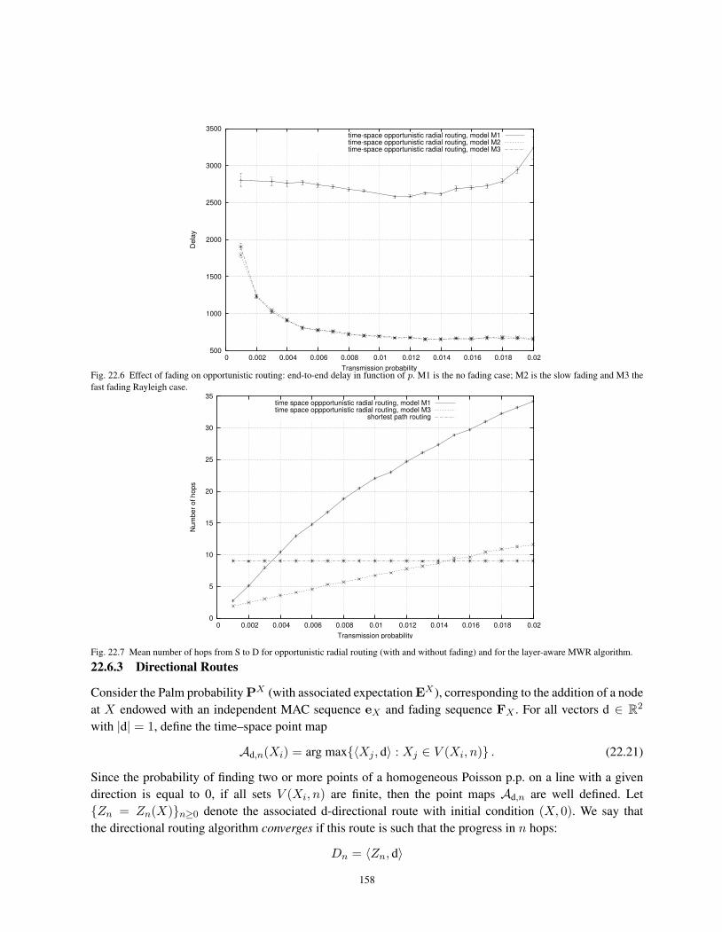
500

1000

1500

2000

2500

3000

3500

0 0.002 0.004 0.006 0.008 0.01 0.012 0.014 0.016 0.018 0.02

Dela

y

Transmission probability

time-space opportunistic radial routing, model M1time-space opportunistic radial routing, model M2time-space opportunistic radial routing, model M3

Fig. 22.6 Effect of fading on opportunistic routing: end-to-end delay in function of p. M1 is the no fading case; M2 is the slow fading and M3 thefast fading Rayleigh case.

0

5

10

15

20

25

30

35

0 0.002 0.004 0.006 0.008 0.01 0.012 0.014 0.016 0.018 0.02

Num

ber

of hops

Transmission probability

time space oppportunistic radial routing, model M1time space oppportunistic radial routing, model M3

shortest path routing

Fig. 22.7 Mean number of hops from S to D for opportunistic radial routing (with and without fading) and for the layer-aware MWR algorithm.

22.6.3 Directional Routes

Consider the Palm probability PX (with associated expectation EX ), corresponding to the addition of a nodeat X endowed with an independent MAC sequence eX and fading sequence FX . For all vectors d ∈ R2

with |d| = 1, define the time–space point map

Ad,n(Xi) = arg max{〈Xj , d〉 : Xj ∈ V (Xi, n)} . (22.21)

Since the probability of finding two or more points of a homogeneous Poisson p.p. on a line with a givendirection is equal to 0, if all sets V (Xi, n) are finite, then the point maps Ad,n are well defined. Let{Zn = Zn(X)}n≥0 denote the associated d-directional route with initial condition (X, 0). We say thatthe directional routing algorithm converges if this route is such that the progress in n hops:

Dn = 〈Zn, d〉

158

0

1000

2000

3000

4000

5000

6000

7000

8000

9000

10000

0 0.002 0.004 0.006 0.008 0.01 0.012 0.014 0.016 0.018 0.02

Local dela

y

Transmission probability

time space oppportunistic radial routing, model M1time space oppportunistic radial routing, model M3

shortest path routing

Fig. 22.8 Mean local delay for opportunistic radial routing (with and without fading) and for the layer-aware MWR algorithm.

tends to∞ when n→∞. Note that Dn+1 ≥ Dn, for all n ≥ 0.We say that the directional routing algorithm progresses if its route is such that |Zn| → ∞when n→∞.

Lemma 22.6.2. Assume that either W ≡ 0 or fading is fast. Then the opportunistic directional routingalgorithm progresses with probability PX one.

Proof. The proof is similar to that of the last lemma and is just sketched.Poisson configurations of points ΦX are locally finite and it is enough to prove that conditionally on

Yn = Xi ∈ ΦX and some appropriate σ-algebra, the event {Zn+1 = Zn } has a probability strictly lessthan 1. For this, one considers the event that node x(= x(Xi), the closest to Xi with 〈x(, d〉 > 〈Xi, d〉,receives the packet transmitted by Xi and one shows that this event has a positive conditional probability.

22.6.4 Scaling Properties of Directional Routes

In the following result P0λ denotes the Palm probability of a Poisson p.p. of intensity λ.

Proposition 22.6.3. Assume OPL 3 and W ≡ 0. Then for any of the fading variation models, the law of thesequence {Zn = Zn(0)}n under P0

λ is the same as that of {Zn/√λ}n under P0

1.

Proof. Note that the distribution of the underlying Poisson p.p. Φ = {Xi)}i under P0λ is the same as the

distribution of Φ(λ) = {(Xi/√λ)}i under P0

1. Moreover, under our assumptions on l and W , the SINR (infact the SIR) is invariant with respect to the scaling Φ(λ) of the p.p. Indeed,

l(|Xi/√λ−Xj/

√λ|) = λβ/2l(|Xi −Xj |)

andIΦn1 (λ)\{Xi/

√λ}(Xj/

√λ) = λβ/2IΦn1 \{Xi}(Xj).

Moreover, the dilation (our scaling) is a conformal mapping (preserves angles). Consequently, the directionalpoint map Ad,n(Xi/

√λ) acting on Φ0(λ) is equal to 1/

√λAd,n(Xi) acting on Φ0

1.

159

It is immediate to extend this to the iterates of order k of the point map. We deduce from this that thedistribution of the Euclidean length of the segments of the directional route scales like 1/

√λ in this case.

Remark 22.6.4. When λ grows large, the network is interference limited and the thermal noise is negligibleand the last scaling law is asymptotically valid. We deduce from this that the number of time steps to progressof some distance r in the direction d asymptotically scales likeCr

√λ at least, whereC is a positive constant.

This is of course compatible with the Gupta and Kumar scaling law.

22.6.5 Related Directional Greedy Point Maps

In connection with (22.21), here are some related time–space directional point maps.

• Largest progress and probability of success:

Ad,n(X) = arg maxXj∈Φ0(n)

{〈Xj −X, d〉pX(Xj)} , (22.22)

where px(y) = Ex,y[δ(x, y, 0) | e0x = 1, e0

y = 0] is the probability of successful transmissionfrom a transmitter at x to a receiver at y ∈ R2, which can be evaluated using the results of §16.2.2.This point map selects the receiver which maximizes the product of the progress in direction dand of the probability of success.• Largest progress and conditional probability of success: this point map maximizes the product

of the progress and of the conditional probability of success given the points of Φ:

Ad,n(X) = arg maxXj∈Φ0(n)

{〈Xj −X, d〉EX [δ(X,Xj , 0) | G, eX = 1, eXj = 0]} , (22.23)

where G is the σ-algebra generated by Φ.• Largest progress and throughput:

Ad,n(X) = arg maxXj∈Φ0(n)

{〈Xj −X, d〉 log

(1 +

F j0 (n)/l(|Xj −X|)W + IΦn1 /{X}(Xj)

)}, (22.24)

where the last term is the throughput of the wireless link from X to Xj .• Smallest hop in a cone:

A(α)d,n(X) = arg min

Xj∈Φ0(n)∩C(X,α,d)

{|Xj −X|} , (22.25)

whereC(x, α, d) = {y ∈ R2, | arg(y − x)− arg(d)| ≤ α/2}

denotes the cone of apex X , direction d and angle α. If α = π, this boils down to smallest hopdirectional routing as defined in (21.13), Chapter 21.

The scaling properties of § 22.6.4 are easily extended to these point maps whenever W ≡ 0. ok?

22.6.6 Route Averages on Radial Time–Space Routes

We conclude with a negative result on the scaling of the delay on all radial time–space routes (and inparticular opportunistic routes) on a Poisson MANET Φ. Let PS,D denote the Palm probability of order 2of Φ at (S,D). Let {An}n by any radial time–space routing to D and let ∆(S,D) denote the end-to-enddelay of the associated route from S to D under PS,D.

160

Corollary 22.6.5. In the MW+M / M model with fast fading and with OPL 3, if the thermal noiseW is bounded

from below by a positive constant, then then for all radial time–space point map to D,

lim|S−D|→∞

ES,D[∆(S,D, Φ)]|S −D|

=∞ , (22.26)

or equivalently the end-to-end delay of a priority packet scales super linearly with distance.

Proof. Optimality implies that∆(S,D) ≥ ∆∗(S,D) ,

with ∆∗(S,D) the optimal number of steps. The result then follows from the second statement of Proposi-tion 22.5.9.

22.7 Conclusion

Here are a few conclusions of practical nature on the packet model over Poisson MANETs.

• Greedy routing on the time–space SINR graph takes information theoretic limitations into ac-count and leverages the physical characteristics of wireless communications. We showed thatthis greedy scheme works well at finite distance, in the sense that it drives a priority packet fromsource to destination in finite time under rather natural conditions.• In contrast, because of the dead end problem, greedy routing on the static random geometric

graph ignores the physical characteristics of wireless links and does not work at finite distance,even in the case where the associated Boolean model percolates and where the source and des-tination nodes belong to the infinite component. Models ignoring these key characteristics mayhence lead to more difficulties than actually needed....• The fact that greedy schemes work well at finite distance should be put in perspective as the mean

end-to-end delays scale super linearly with distance in many practical cases. In a sense, the deadend problem hits back in the greedy time–space scenario: the fact that the mean local delays scalein a more than linear way with distance is again primarily due to the very large number of timesteps that the packet needs to progress from certain relay nodes along the route.

This chapter opens many questions on the packet model. For instance, we are currently working on thefollowing problems:

• In the case of a Poisson MANET with an added periodic infrastructure, does there exist greedyrouting schemes on the time–space SINR graph with delays scaling linearly with distance or witha positive asymptotic velocity?• In the Poisson MANET case, what is the rate at which delays grows to infinity with distance?• How can one integrate packet contention and queueing disciplines (other than preemptive prior-

ity)?

The chapter was centered on the packet model but it should be clear that most of the above questions (optimalroutes, greedy schemes) have natural counter parts in the Shannon capacity model.

Let us conclude by stressing that, more generally, SINR routes on a p.p., both optimal and suboptimal,form fascinating new objects of stochastic geometry which generate a large number of questions at theinterface between communications and probability theory.

161

Bibliographical Notes on Part V

The ergodic properties of MWR in Chapter 20 are directly related to first-passage percolation, an issueextensively studied in the mathematical literature. For instance, first passage percolation on the completePoisson p.p. graph, with weights w(x, y) = |x − y|α, for α > 1 was studied in (Howard and Newman1997). The existence of the Euclidean minimal spanning tree for infinite Poisson point patterns is consideredin (Aldous and Steele 1992). See also (Howard and Newman 1997).

Geographic routing is discussed in (Karp 2000). To the best of our knowledge, the first paper on theperformance evaluation of routing algorithms using spatial p.p. is (Takagi and Kleinrock 1984), where whatwe call directional routing was analyzed. Protocols where one minimizes the remaining distance to desti-nation are considered in (Stojmenovic and Lin 2001a; Stojmenovic and Lin 2001b). The analysis of greedygeographic routing in Chapter 21 is based on (Baccelli and Bordenave 2007) and on (Bordenave 2006). Therouting paradox was first observed in (Baccelli and Bordenave 2007) within the context of smallest hoprouting.

To the best of the authors’ knowledge, the studies presented in (Blum, He, Son, and Stankovic 2003)and (Baccelli, Blaszczyszyn, and Muhlethaler 2003) were the first papers where geographic routing wasused in combination with a MAC protocol and where an opportunistic self election of relays was pro-posed for packets traveling from an origin to a destination node. (Biswas and Morris 2005) also uses thisidea. Both protocols presented in (Blum, He, Son, and Stankovic 2003) and (Biswas and Morris 2005) use802.11 like MAC access solution where the acknowledgement scheme is modified to allow the selection ofthe relay. Chapter 22 is primarily based on (Baccelli, Błaszczyszyn, and Mirsadeghi 2009) and (Baccelli,Blaszczyszyn, and Muhlethaler 2009b). In relation with the variants considered in § 22.6.5, let us quote(Weber, Jindal, Ganti, and Haenggi 2008), where a routing scheme based on the the longest outgoing edgein the SINR graph is studied.

The question of the speed of the delivery of information in large wireless ad-hoc networks was studiedrecently in (Ganti and Haenggi 2009; Jacquet, Mans, Muhlethaler, and Rodolakis 2009). In these papersthe so called delay-tolerant networks are considered and modeled by a spatial SINR or SNR graph withno time dimension. In these models, the time constant (defined there as the asymptotic ratio of the graphdistance to the Euclidean distance) is announced to be finite, even in the pure Poisson case. The reason for

163

the (apparently) different performance of these models lays in the fact that they do not take into accountthe time required for a successful transmission from a given node in the evaluation of the end-to-end de-lay. The heavy-tailness of this time (cf. Section 17.5.6) makes the time constant infinite in the space-timePoisson scenario. This is not so surprising observation in view of (Jelenkovic and Tan 2007a; Jelenkovicand Tan 2007b), although the physical phenomena at hand are quite different there; in our model the spatialirregularities in the ad-hoc network play a role similar to that of the file size variability in papers cited above.

164

Part VI

Appendix: Wireless Protocols andArchitectures

165

The aim of this part is to give a compact survey on the statistical properties of channels which arecommonly used in the analysis of wireless networks. The main focus will be on the principles and most ofthe fine points associated with technological aspects will not be discussed here.

In Chapter 23, we describe scattering and fading channels; this can be seen as the very first level ofstatistical modeling within this context. The presence of scatterers and the resulting multipath propagationtogether with the mobility of the source or the destination lead to the definition of a variety of fading channelsincluding the Rayleigh and Rician models.

Chapter 24 will then outline the theory of detection for such channels with a main emphasis on pointto point channels in scenarios involving a collection of simultaneous transmissions taking place in somedomain. The case of direct-sequence spread-spectrum, where the interference created by other transmissionscan be seen as noise for any given point to point channel, will be discussed, again at the level of principles.This discussion will in particular lead to a comprehensive explanation of the key role played by the SINR insuch a scenario.

The aim of Chapter 25 is to provide a bestiary of classical network architectures and protocols whichwill be used as simple illustrating examples in Part I in Volume I and to which we will return in more detailsin the parts which follow. We will in particular survey the basic medium access control protocols used toorganize the competition between such a collection of transmissions and on multi-hop routing within thiscontext. Among the examples of network architectures which will be outlined, let us quote mobile ad hocnetworks, wifi mesh networks and cellular access networks.

These chapters rely on a variety of scientific domains: physics, with questions pertaining to propagation,the Doppler effect, scattering etc.; information theory, with questions bearing on additive white Gaussiannoise channels, detection theory etc. and finally networking, with routing algorithms or protocols for theorganization of concurrent transmissions sharing a common medium.

All these ingredients are necessary for a full understanding of the main findings concerning SINR, whichare the basis of most of the models of the monograph.

166

23Radio Wave Propagation

In this chapter we will be interested in the propagation of an electromagnetic signal in space, where it is ab-sorbed and reflected by many, possibly moving, obstacles. In such a context, solving and even establishingthe detailed electromagnetic field equations is not feasible. However, for wireless communication engineer-ing, it is often enough to use some macroscopic model that predicts the relationship between transmittedand received signals in a statistical way. In such a model, the impact of the unknown locations of variousobjects which absorb and reflect the signal is represented by some random transformation of the signal.Most macroscopic models just give the mean signal power attenuation for a given distance. They describethe average signal power attenuation for different environments (e.g. an urban environment, the countryside,etc.). Refined statistical models also give the fluctuations of the signal power attenuation around this meanprofile. These models will be used in the analysis of the higher layers (detection, MAC, routing, etc).

23.1 Mean Power Attenuation

Mean power attenuation is concerned with the macroscopic description of the decrease of the signal powerwith the distance between the transmitter and receiver. We will first give two motivating examples and thenintroduce a few simple parametric models.

23.1.1 Motivating Examples

Digital radio communications are based on electromagnetic waves. Assume that the electric signal trans-mitted at time t by an antenna located at the origin of the three dimensional Euclidean space is of the formS(t) = cos(2πft). If f is equal to 1 GHz, the wavelength is λ = c/f , where c is the speed of light, that isλ ∼ 30 cm.

Example 23.1.1 (Free Space Propagation). The simplest propagation model is the free space model whichstates that the signal received at the point (r, θ, ψ) at time t is

Rr,θ,ψ(t) =α(θ, ψ)r

cos(2πf(t− r/c)) =α(θ, ψ)r

cos(2πft− φ), (23.1)

167

where α = α(θ, ψ) denotes the gain of the antenna in the (θ, ψ) direction and where the signal phase φis 2πr/λ. The 1/r term in the amplitude stems from a simple energy conservation law. Hence the powerreceived at distance r is proportional to 1/r2. In the particular case of omni-directional antennas, α(θ, ψ) isconstant.

In the free space model, the power of the signal is attenuated proportionally to 1/r2. In practice however,when the traversed space is not empty, power decreases much faster. We will explain this in the followingexample, where we take into account the reflection of the signal on the ground, and where power decreasesin 1/r4.

Example 23.1.2 (Ground Reflection). If the transmitter and the receiver are above the ground, then oneshould both consider the direct path with length r1 and the reflected path with length r2. Let r denote theground distance between the transmitter and the receiver. Then for r large, r2 − r1 ≈ b/r where b is aconstant that depends on the heights of the transmitter and the receiver. The received signal is then

Rr(t) ≈ α(θ, ψ)(

1r1

cos(2πf(t− r1/c))−1r2

cos(2πf(t− r2/c))), (23.2)

which is easily seen to be of the order of 1/r2 in the far-field, namely when r is large. Hence the power isproportional to 1/r4. The minus sign in the second term of the last equation stems from the fact that the signof the electric field is reversed by the ground reflection; this explains why the two waves interact here in adestructive way.

In view of the two simple scenarios described above, it should be clear that an exact analysis of thepropagation of the signal in a “real” scenario with many obstacles and reflections would be extremely com-plicated. Fortunately this is not necessary as some statistical models of the attenuation of power are oftensufficient for the purpose of radio communication engineering.

23.1.2 Mean Power Attenuation Models

Linked to the two models described above, it is customary to consider the following general macroscopicdistance-and-angle dependent path-gain model according to which the power of the signal received at dis-tance r and in the direction θ, ψ (respectively referred to as the azimuth and the tilt) is equal to

σ2 = σ2(r, θ, ψ) =α2(θ, ψ)l(r)

, (23.3)

where

• l is the omni-directional (isotropic) path loss function 1 (OPL),• α2(θ, ψ) denotes the value of the mean normalized radiation pattern (RP) in the direction θ, ψ;

it takes into account the transmitter and receiver antenna gains.

1This definition of path loss is natural: if the path loss is large, the received signal has a low power.

168

α2(θ)

0

0.2

0.4

0.6

0.8

1

–3 –2 –1 1 2 3

θ

–1

–0.5

0

0.5

1

–1 –0.5 0.5 1

α2(θ)

0

0.2

0.4

0.6

0.8

1

–3 –2 –1 1 2 3

θ

–1

–0.5

0

0.5

1

–1 –0.5 0.5 1

Fig. 23.1 Top: approximation of RP1 by RP2 with θ1 = 112π, θ2 = 2

3π; Cartesian and polar plots. Bottom: in boldface/red, perfect RP modeled

by RP2 with θ1 → π/3− and θ2 → π/3+; Cartesian and polar plots.

Example 23.1.3 (Omni-directional path-loss function). The following examples of isotropic path-lossfunctions will be considered:

(OPL 1) l(r) = (Amax(r0, r))β ,(OPL 2) l(r) = (1 +Ar)β ,(OPL 3) l(r) = (Ar)β ,

for some A > 0, r0 > 0 and β > 2, where β is called the path-loss exponent. Note that OPL3 is a simplifiedmodel making no sense for r close to 0. However it is reasonable for r bounded away from 0. It is thusimportant to use it is with caution. All three cases OPL1–OPL3 give similar values for r > r0 and/or whenAr is large.

Example 23.1.4 (Planar radiation patterns *). We will concentrate on planar RPs, namely RPs such thatα2(θ, ψ) = α2(θ). Apart from a few exceptions, we will use

(RP0) α2 ≡ 1, which corresponds to perfect omni-directional radiation.

169

–10

–5

0

5

10

y

–10 –5 5 10

x

–10

–5

0

5

10

y

–10 –5 5 10

x

Fig. 23.2 Equal-strength power sets (path-loss level sets) for (23.3) with omni-directional attenuation OPL 2 withA = 1000, β = 3, and radiationpatterns RP1 (left), RP2; θ1 = 1

12π, θ2 = 2

3π (right). The contours represent the levels t = {100, 110, 120}dB.

As examples of truly directional RPs we will consider patterns with a 3dB azimuth beam-width of 120◦.Here are two mathematical models with this property:

(RP1) is defined by

α2(θ) =∣∣∣∣sin(ωθ)

ωθ

∣∣∣∣ |θ| ≤ π ,

where ω = 1.81 is chosen such that α2(

13π)

= 12 = 3dB.

(RP2) is defined by

α2(θ) =

1 for |θ| ≤ θ1,∣∣∣∣1− |θ| − θ1

2(π/3− θ1)

∣∣∣∣ for θ1 < |θ| ≤ θ2,∣∣∣∣1− |θ2| − θ1

2(π/3− θ1)

∣∣∣∣ for θ2 < |θ| ≤ π,

where 0 < θ1 <13π < θ2 < π and θ1 + θ2 >

23π are such that α2

(13π)

= 12 = 3dB.

Figure 23.1 illustrates these RP models. Notice that in the above definitions,

• The main and the first secondary lobes can be taken into account.• In RP2, if one lets θ1 → π/3− and θ2 → π/3+ in such a way that (θ2−π/3)/(π/3−θ1)→ 1+,

then RP2 tends to a perfect coverage of the sector (−π/3, π/3).• If θ1 = 1

12π and θ2 = 23π, then RP2 is a piecewise linear approximation of RP1 (these parameters

are chosen by “visual inspection”).

Figure 23.2 depicts the equal-signal-strength set (or path-gain level-set) {y ∈ R2 : σ2(|y|, arg(y)) = t}associated with a few levels t. The antenna has its main lobe in the direction θ = 0 (one also says that itsazimuth is equal to 0) and is located at 0 ∈ R2. We consider both RP 1 and RP 2 and assume l(r) is givenby OPL 2. One sees that a piece-wise-linear radiation pattern RP 1 can be used to approximate RP 2.

170

23.2 Random Fading

The mean model of power attenuation described in the previous section does not capture the importantphenomenon of the variation of the signal power over short distances (of the order of the wavelength) andin time. We will explain the nature of these variations in a few examples and then show a stochastic modelwhich, in some cases, can capture this phenomenon.

23.2.1 Motivating Examples

When the transmitted signal propagates to the receiver, it may actually meet a collection of different objects(called scatterers) on its way, and they may reflect it. This leads to the situation where several differentcopies of the signal are received, each of them propagated along a specific path.

Example 23.2.1 (Scattering and Multipath Fading). Assume for simplicity that there are two paths: path1 is the direct path with distance r1 = r; path 2 stems from the reflection of the signal on a wall at distanced > r from the transmitter and orthogonal to the direction of the direct path, so that r2 = 2d− r. Hence thereceived signal is equal to

R(t) =α

rcos(

2πf(t− r

c

))− α

2d− rcos(

2πf(t− 2d− r

c

)).

The received signal is hence the superposition of two waves with the same frequency f but with a phasedifference of ∆φ = π + 4πf(d − r)/c = π + 4π(d − r)/λ. When ∆φ is an even (resp. odd) multipleinteger of π, the two waves add constructively (resp. destructively). This means that changing r by λ/4 canchange the received signal strength from a local maximum to a local minimum. Note however, that if thedistance between two reception locations is significantly less than λ/4 the strength of the received signalis unchanged. This coherence distance ∆ = λ/4 is of the order of 10 cm when f = 1 GHz. Similarly,changing the frequency f by c/(4(d − r)) leads from a peak to a valley of the signal at a given location.However, if the frequency change is significantly smaller than this value, the signal strength does not vary toomuch. Thus the bandwidth c/(2(d− r)) is called the coherence bandwidth. The reciprocal of the coherencebandwidth is called the delay spread.

The following example shows how mobility (of transmitter, receiver or scatterers) impacts the variationof the signal strength in time.

Example 23.2.2 (Motion and Small Scale Fading). We assume that the receiver is moving at a speed vand in some direction which do not vary over the time interval considered. In the open space model the(direct) path length varies with time as

r (t) = r + vt cos(γ),

where γ is the angle of the path and the receiver motion and where r = r (0). Hence (23.1) should bereplaced by

R(t) =α(θ(t), ψ(t))

r(t)cos (2πft− φ (t)) , (23.4)

where

φ (t) =2πr (t)λ

= φ+v cos(γ)

c2πft.

171

with φ = 2πfr/c = 2πr/λ. If we can assume that the path gain does not change significantly within thetime intervals of interest, then

R(t) ∼ α(θ, ψ)r

cos(

2πf(

1− v cos(γ)c

)t− φ

), (23.5)

where we observe the classical Doppler shift D = −vf cos(γ)/c, i.e. the change of the frequency from f tof +D.

Let us revisit now our simple wall reflection scenario of Example 23.2.1 with the receiver moving to-wards the wall. Path 1 is the direct path with γ1 = 0 (the motion and the transmitter–receiver vectors arecollinear) and r1(t) = r + vt; path 2 stems from the reflection of the signal on the wall and γ2 = π andr2(t) = 2d − r − vt. Then the time between a constructive and a destructive phase combination is c/4vf .More precisely,

R(t) =α

r + vtcos(

2πf((

1− v

c

)t− r

c

))− α

2d− r − vtcos(

2πf((

1 +v

c

)t− 2d− r

c

)). (23.6)

When the mobile is close to the wall, r + vt and 2d − r − vt are of the same order (on a sufficiently smalltime interval) and

R(t) ∼ 2αr + vt

sin(

2πf(t− d

c

))sin(

2πf(vt

c+r − dc

)).

We see that the received signal is the multiplication of some high frequency wave sin(2πf(t − d/c)) (werecall that f is of the order of the GHz) by some low frequency (envelope) wave at fv/c. This means that thestrength of the signal received by this mobile antenna varies in time with the frequency fv/c. The reciprocalof this value, c/vf , is called the coherence time. One can say that the power of the received signal remainsconstant in time intervals significantly smaller than this coherence time. For example if the velocity is of theorder of 60 km/h, fv/c is of the order of 55Hz and the coherence time of the order of 18ms.

In cases with more reflectors, one observes several Doppler shifts of the frequency f . Denote by Dn thatof path n. Then, the Doppler spread is defined as

Ds = supnDn − inf

nDn.

The envelope ofR(t) varies at a time scale of the order of 1/Ds. On time intervals significantly smaller thanthe coherence time Tc = 1/(4Ds), there is no sizable variation of the strength of the received signal. Thistime scale is small compared to that of the variations of the path gain induced by motion due to large scalefading. Hence the terminology of small scale fading.

It should also be clear that a similar phenomenon is also present when the transmitter and/or scatterersare mobile.

An exact analysis of the small time/space scale variations of the signal strength described in the aboveexamples would be too complicated in a real life situation. The stochastic models described below are bettersuited for the description of these phenomena.

23.2.2 Random Scatterers

Consider many static or moving scatterers giving N different copies of the transmitted signal, each propa-gating along a specific path. A signal traveling on path n with length rn arrives with some delay τn = rn/c.

172

Therefore the received signal is

RN (t) =N∑n=1

ξn cos (2πf(t− τn)) =N∑n=1

ξn cos (2πft− φn) , (23.7)

where in the simplest case, φn = 2πfτn and ξn = bnαnrn

, with αn the antenna gain in the direction of path nand bn the variable with value +1 or −1 depending on the number of reflections on path n. More complexscenarios can be considered like

• the case of mobility where φn depends on t via the Doppler shift Dn of path n: φn(t) = φn +2πDnt (cf. (23.4));• the case where each path is reflected on the ground so that when aggregating the effect of path n

and its reflection, we get a formula of the form ξn = bnαnr2n

.

Far-field Assumptions. In the case where transmitter, receiver and scatterers are fixed, the path parametersdo not vary with time t and φn = 2πrn/λ. If we suppose now that rn � λ, which corresponds to the socalled far-field model, then it is reasonable to assume that

• rn/λ − brn/λc is uniformly distributed in [0, 1), so that φn is uniformly distributed in [0, 2π)and the phases {φn} are independent;• the random variables ξn are i.i.d.; and• the sequences {φn} and {ξn} are independent.

Note that under these assumptions, variables bn can be removed in (23.7) without altering the law of thereceived signal R(t).

Claim 23.2.3. Under the above far-field assumptions, the received signal {R(t)} is a centered stationarystochastic process with auto-correlation function

C (s) =12

∑n

E[ξ2n

]cos (2πfs) . (23.8)

Remark: Note that 12 = 1/(2π)

∫ 2π0 cos2(t) dt is the mean power of the transmitted signal and E[ξ2

n] = a2

can be interpreted as the value of the mean path-gain function at a given location; cf. the model aroundEquation (23.3).

Proof. Stationarity stems from the fact that each term of the sum is stationary, which follows from theuniform phase assumption and the independence assumption. The first moment property is clear. Using thefact that the random phases are independent and uniform, one gets that the auto-correlation is

E[R(t+ s)R(t)] =∑n,k

E [ξn cos (2πf (t+ s)− φn) ξk cos (2πft− φk)]

=∑n

E[ξ2n

]E [cos (2πf (t+ s)− φn) cos (2πft− φn)]

=12

∑n

E[ξ2n

]cos (2πfs) .

173

This property extends to the more complex settings considered so far, whenever the uniform phase andindependence properties are satisfied.

Large Number of Random Scatterers in the Far-field. We now study what happens with themodel (23.7) when the number of paths N is large. The setting is that of the far-field model. Moreover,we assume that

• ξn = ξN,n, n = 1, . . . , N , N ≥ 1 are such that the total power of the received signal

E[R(t)2] = C (0) =12

N∑n=1

E[ξ2N,n

]= a2/2 (23.9)

is the same for all N .

A typical example is that where ξN,n = 1√NYn, where {Yn}n∈N is an i.i.d. sequence of positive random vari-

ables with finite second moment a2/2. In this particular case, the central limit theorem implies that RN (t)converges in distribution to a centered Gaussian random variable when N tends to infinity. More gener-ally, we have the following result when we assume that the path gains are independent but not necessarilyidentically distributed.

Claim 23.2.4. If the condition

limN→∞

N∑n=1

E[ξ2N,n1 {ξN,n ≥ εa}

]= 0, for all ε > 0 (23.10)

is satisfied, then RN (t) converges in distribution to a Gaussian random variable N (0, a2) when N → ∞.Similarly, for all k ≥ 1 and for all t1, . . . , tk and β1, . . . , βk ∈ R, the random variable

∑kj=1 βjR(tj)

converges in distribution to a Gaussian random variable when N →∞.

Proof. We apply the Lindeberg version of the central limit theorem (Billingsley 1995, Theorem 27.1 p.359).Let

XN,n = ξN,n cos (2πft− φn) .

SinceX2N,n1 {|[XN,n| ≥ εa} ≤ ξ2

N,n1 {ξN,n ≥ εa}

andN∑n=1

E[X2N,n

]=

12

N∑n=1

E[ξ2N,n

]=a2

2,

Condition (23.10) implies the Lindeberg condition

limN→∞

N∑n=1

E[X2N,n1 {XN,n ≥ εa}

]= 0, for all ε > 0

which allows one to apply Lindeberg’s theorem (Billingsley 1995, Theorem 27.1 p.359).

174

23.2.3 Quadrature Amplitude Modulation (QAM)

Up to now we have considered radio transmission of a simple high frequency sinusoidal signal at the carrierfrequency f = fc. In reality, a low frequency signal S(b)(t) called baseband signal, to be communicatedover the radio, is first transformed into some equivalent high frequency passband signal S(t) which is thentransmitted, propagated, received as R(t) and transformed back to the low frequency baseband represen-tation R(b)(t) of R(t). This procedure is called Quadrature Amplitude Modulation. We now analyze theimpact of our previous stochastic assumptions (large number of random scatterers, far-field) on the variationof the baseband representation of the signal at the receiver.

Denote by S(t) the passband signal and by S(b)(t) the baseband signal. Denote by S(f) the Fouriertransform of S(t) and by S(b)(f) that of S(b)(t), which we assume to exist. The one to one correspondencebetween the two signals is best described through the following relations between their Fourier transforms:

S(f) =1√2

[S(b)(f − fc) +

(S(b)

)∗(−f − fc)

](23.11)

andS(b)(f) =

√2S(fc + f)1{f + fc > 0}. (23.12)

The normalization by√

2 is introduced so that S and S(b) have the same power. We assume that S(b)(f)vanishes for frequencies f outside the baseband [−W/2,W/2] for some bandwidth W/2 < fc, so that S(f)vanishes for frequencies f outside the passband [−W/2 + fc,W/2 + fc].

The fact that S(−f) = S∗(f) shows that S(t) is real, whereas the baseband signal is complex-valued:

S(b)(t) = S(b)I (t) + iS

(b)Q (t)

with S(b)I (t) the in phase component and S(b)

Q (t) the quadrature component. This terminology stems fromthe following time domain up-conversion formula (which follows from (23.11)):

S(t) =√

2S(b)I (t) cos(2πfct)−

√2S(b)

Q (t) sin(2πfct) =√

2R(S(b)(t)ei2πfct

), (23.13)

whereR denotes the real part.Assuming the channel model (23.7), if the passband signal S(t) is transmitted, then the received signal

is equal to

R(t) =√

2R(b)I (t) cos(2πfct)−

√2R(b)

Q (t) sin(2πfct) =N∑n=1

ξnS(t− τn)

=√

2

(N∑n=1

ξn

(S

(b)I (t− τn) cos(2πτn)− S(b)

Q (t− τn) sin(2πτn)))

cos(2πfct)

+√

2

(N∑n=1

ξn

(S

(b)I (t− τn) sin(2πτn) + S

(b)Q (t− τn

)cos(2πτn))

)sin(2πfct) ,

where we used (23.13). Simple trigonometry arguments show that the solution to this equation with a lowfrequency is

R(b)N (t) =

N∑n=1

ξn,Ne−i2πτnS(b)(t− τn). (23.14)

175

One can prove a Central Limit Theorem forR(b)N (t) under conditions similar to (23.10), namely one can show

that when N → ∞, the random variable R(b)N (t) converges in distribution to a complex-valued Gaussian

random variable ZI(t) + iZQ(t) (for more on complex-valued Gaussian random variables, see §24.1). Itis beyond our scope to work out such conditions in detail. Instead, we exemplify this convergence in thefollowing simple case:

Example 23.2.5. Since S(b) is a low frequency signal, it is reasonable to assume for simplicity that it is(piecewise) constant. Then S(b)(t− τn) = S(b). We recall that, under a far-field assumption, ξn = ξn,N andφn = 2πτn are independent and φn is uniformly distributed on [0, 2π). Consequently E[ξnS(b)e−iφn ] =S(b)E[ξn]E[e−iφn ] = 0. This shows that E[ZI ] = E[ZQ] = 0. Let us now calculate the covariance of thereal and imaginary parts of R(b)

N . From (23.14) by independence of the paths

E[R(R(b)

N )I(R(b)N )]

=N∑n=1

E[ξ2n,N ]E

[R(S(b)e−iφn

)I(S(b)e−iφn

)]= 0 ,

where I denotes the imaginary part, since

E[R(S(b)e−iφn

)I(S(b)e−iφn

)]=

((I(S(b)))2 − (R(S(b)))2

)E[sin 2φn

2

]+ I(S(b))R(S(b))E[cos 2φn] = 0 .

Hence ZI and ZQ are uncorrelated and thus independent, provided they form a Gaussian vector. Note alsothat under the assumption

∑Nn=1 ξ

2n,N = a2, we have E[Z2

I + Z2Q] = |S(b)|2a2, namely the mean power of

the baseband signal is the product of |S(b)|2, the power of the baseband signal at the transmitter, and of a2,the mean power attenuation.

Remark: Since ZI and ZQ are independent N (0, |S(b)|2 a2

2 ) random variables (where N (µ, σ2) denotesthe Gaussian law of mean µ and variance σ2), the power Z2

I + Z2Q of the received baseband signal has a χ2

2

distribution (up to a multiplicative constant). More precisely it is an exponential random variable with meana2|S(b)|2 (and its square root has a Rayleigh distribution with parameter a2|S(b)|2).

Inspired by the above remark we will introduce now a basic stochastic model for variations of the re-ceived power.

23.2.4 Rayleigh Fading and its Extensions

In Section 23.1.2 we have modeled the mean received signal power by some fraction a2 = a2(r, θ, ψ) of theemitted power. This mean fraction is a function of the distance between the transmitter and the receiver andof certain angles θ, ψ associated with antenna azimuths and tilts. The last examples lead to the followingnatural random model for the law of the received power.

Definition 23.2.6. We say that the wireless channel exhibits Rayleigh fading if the received power is equalto Pa2F , where P is the power of the transmitted signal, a2 is the mean attenuation function and F isexponential random variable with mean 1.

Note that this definition is only valid when QAM is used in the far-field and when there are many scatterers.In the situation where an important fraction of the power is received on the line-of-sight path, the followingmodel is more pertinent:

176

Definition 23.2.7. We say that the wireless channel exhibits Rician fading if the received power is equal toPa2κ/(κ+ 1) +F/(κ+ 1), where κ/(κ+ 1) is the fraction of the mean power received on the line-of-sightpath and P , a2 and F are as for Rayleigh fading.

When several groups of paths can be distinguished, each group contributing to an exponential power with adifferent mean, one can use a Nakagami fading model (see (Stuber 2001)).

23.3 Conclusion

Note that the above stochastic models give the distribution of the fading F at a given location and at agiven time with respect to some given transmitter. It is difficult to model the fading F = F (t, x, f) in thetime-space-frequency domain x ∈ R3, t ∈ R, f ∈ R+. However, the following remarks will be useful:

• If |x − y| � ∆, where ∆ is the coherence distance (see Example 23.2.1), then one can assumethat F (t, x) = F (t, y).• If |t − s| � Tc, where Tc is the coherence time (see Example 23.2.2), then one can assume thatF (t, x) = F (s, x).• If |t− s| � Tc or |x− y| � ∆ then F (t, x) and F (s, y) can be considered as independent ran-

dom variables. Since the scattering obstacles are different for (sufficiently separated) transmitter–receiver pairs, it makes sense to assume that these random variables are independent for all suchpairs.• Fading depends on the signal frequency. However if the change of frequency is significantly

smaller than the coherence bandwidth (see Example 23.2.2) then the received power at a givenlocation and time does not vary too much.

177

24Signal Detection

The aim of this chapter is to show through a few basic examples how signal to noise and signal to noiseand interference ratios determine error probability and hence throughput on the multipath wireless chan-nels described in the preceding chapter. Detection will be considered in a discrete channel model based onthe sampling theorem which is described first. We start with a few well known facts on complex–valuedGaussian vectors.

24.1 Complex Gaussian Vectors

A complex–valued random vector of dimension n is said to be Gaussian if its real and imaginary parts forma Gaussian vector of dimension 2n. A complex–valued random vector X of dimension n is said to be

• circular-symmetric if eiθX has the same law as X for all θ;• isotropic if for all unitary1 transformations U of Cn, UX has the same law as X .

A complex–valued Gaussian scalar is circular-symmetric iff its real and imaginary parts are i.i.d. and cen-tered. We will denote by N C(0, σ2) this distribution when the variance of the real (or imaginary) part isσ2/2.

A vector of Cn with i.i.d. N C(0, σ2) components is both circular-symmetric and isotropic.

24.2 Discrete Baseband Representation

24.2.1 Linear Model

Assume that the mapping which gives R from S is of the form

R(t) =∑n

ξn(t)S(t− rn(t)

c

)(24.1)

1U is unitary if (Ut)∗U = I with Ut the transpose of U and U∗ its complex conjugate.

179

with ξn(t) = bnαn(t)/rn(t), which is a time dependent version of (23.7), Chapter 23. Let S(b)(t) andR(b)(t) denote the baseband representation of S and R respectively. By calculations similar to those madein § 23.2.2, we conclude that the mapping which gives R(b) from S(b) is

R(b)(t) =∑n

βn(t)S(b)

(t− rn(t)

c

), (24.2)

whereβn(t) = ξn(t)e−2πifc

rn(t)c . (24.3)

Assume now that S(b)(t) is integrable, continuous and band-limited to W . Since the Fourier transformof S(b)(t) vanishes outside [−W/2,W/2], the sampling theorem (Bremaud 2002) states that there is no lossof information in sampling S(b)(t) every 1/W seconds and that

S(b)(t) =∑k∈Z

S(b)[k]sinc(Wt− k), (24.4)

with S(b)[k] = S(b)(k/W ) the k-th sample and

sinc(t) =sin(πt)πt

.

Hence (24.2) can be rewritten as

R(b)(t) =∑n

βn(t)∑k

S(b)[k]sinc(Wt−W rn(t)c− k)

=∑k

S(b)[k]∑n

βn(t)sinc(Wt−W rn(t)c− k), (24.5)

provided the series is absolutely convergent. Thus, the m-th sample of R(b)(t) at multiples of 1/W is

R(b)[m] =∑k

S(b)[k]∑n

βn(m/W ) sinc(m− k −W rn(m/W )

c

).

Substituting m− k = l, we finally get the following discrete time filter:

R(b)[m] =∑l

Hl[m]S(b)[m− l], (24.6)

where

Hl[m] =∑n

βn(m/W ) sinc(l −W rn(m/W )

c

). (24.7)

This map from the sequence of complex input symbols {S(b)[k]}k which are produced at rate W at thetransmitter to the set of output symbols {R(b)[k]}k at the receiver, takes into account both the modulation ofthe signal to its passband version at the transmitter, the propagation of the resulting signal from transmitterto receiver, the conversion back to the baseband at the receiver, and finally the sampling there.

A few important remarks are in order:

• If the functions ξn(.) are constant (as in e.g. Example 23.2.1), then Hl[m] ≡ Hl and the discretelinear filter is time-invariant.

180

• Using the shape of the sinc function, one sees from (24.7) thatHl predominantly selects the pathswith a delay of the order of l/W .• If the mapping which gives R from S is given by

R(t) =∑n

bn(t)αn(t)rn(t)

S

(t− rn(t)

c

)+W (t), (24.8)

where W (t) is a stationary 0-mean additive white Gaussian noise with variance σ2, namely aGaussian process such that E(W (t)W (s)) = σ2

2 1{t = s}, then a similar construction gives thefollowing input–output map:

R(b)[m] =∑l

Hl[m]S(b)[m− l] +W [m], (24.9)

where W [m] is an i.i.d. sequence of N C(0, σ2) random variables.

24.2.2 Time Coherence

From (24.2)–(24.3) and from the fact that ξn(t) and rn(t) vary slowly, one gets that at time t, the linearmap which gives R(b) from S(b) is approximately time invariant on time scales significantly smaller than thecoherence time Tc = 1/(4Ds), where Ds is the Doppler spread at time t, which is defined as

Ds =fcc

maxn,n′|rn(t)− rn′(t)|,

where the maximum bears on all pairs of paths (cf. Example 23.2.1). Similarly, one gets from (24.7) that forall l, the function Hl[m] is approximately a constant in m when m varies over an interval of length less thanWTc.

24.2.3 Frequency Coherence

LetTd = max

n,n′2π

1c|rn(t)− rn′(t)|

be the multipath delay spread at time t. It is natural to define the coherence bandwidth Wc at time t asWc = 1/Td. If the bandwidth of the input W is significantly less than the coherence bandwidth Wc, then thedelay spread is significantly less than the symbol time 1/W so that only one term l0 has to be considered inthe sum (24.9). This case is called flat fading. In most applications, Td is of the order of a microsecond. Thisgives an upper bound on the bandwidth of the input for flat fading to be an acceptable model. The simplestflat fading model is

R(b)[m] = H0[m]S(b)[m] +W [m]. (24.10)

24.2.4 Statistical Model

Consider now the far field of §23.2.2. Since fcrn(t)/c is large, it makes sense to assume that the phase onpath n, which is this quantity modulo 2π, is uniformly distributed on (0, 2π) at any time t. Hence for all n,l and m, the random variable

Xn = ξn(m/W )e−2πifcrn(m/W )

c sinc(l −W rn(m/W )

c

),

181

which occurs in the definition of Hl[m] (24.7), is a circular symmetric complex–valued random variable.Assume that N , the number of scatterers, is large and that the contributions of all paths (path gains andphases) are independent and satisfy a condition of the Lindeberg type. Then for all l andm, the lawHl[m] =∑N

n=1Xn is asymptotically Gaussian circular symmetric (and in particular centered). Hence |Hl[m]| has aRayleigh distribution with a parameter σl that depends on l but not on m, at least for time scales where thedistances rn(.) do not vary significantly.

Not surprisingly, the autocorrelation of the Hl[m] sequence:

Rl(n) = E(Hl[m]Hl[m+ n])

can be shown to become small for values n such that n/W is significantly larger than K/Ds with Ds theDoppler shift of the channel and K some constant, which is a rephrasing of the notion of coherence timealready discussed above.

24.3 Detection

24.3.1 Coherent Detection

Assume a flat fading scenario of the form

Y = HX +W,

where

• X = X[m] and Y = Y [m] are complex–valued;• W = W [m] is N C(0, σ2);• H = H[m] (in the case of Rayleigh fading, H is N C(0, g2)).

Assume H = H[m] to be known by the receiver (this is the coherent detection case). In practice, this canbe implemented using some pilot signal and requires that H[m] does not change too fast with m. Moreprecisely this requires that WTc be large compared to 1 (for instance due to a large coherence time).

Assume antipodal signaling, namely the signal to be transmitted is real and either +a or −a with proba-bility 1

2 .

Remark: Here, and throughout this section, in order to take into account the effect of the distance betweenemitter and receiver, the value of a2 should be interpreted as the mean power of the signal at the receiver.In general, it depends on the value of the emitted power, distance and antenna parameters; cf. the modelsdiscussed in Section 23.1. So one may see the result of this section as given for the emitted power P = 1,mean path-gain equal to a2 and the random channel fading at time m equal to H .

Claim 24.3.1. Under the foregoing assumptions, the maximum likelihood estimator leads to error probabil-ity

Q

(√2a2|H|2σ2

), (24.11)

where Q is the tail of the cumulative distribution function of the N (0, 1) density.

182

Proof. Given that H = h, if the complex number y is received, the maximum likelihood estimator gives +aif

|y − ah| < |y + ah|.

Let v denote the complex number v = h/|h|. The last inequality is equivalent to

|v∗y − a|h| | < |v∗y + a|h| |,

where v∗ denotes the complex conjugate of v. Since a|h| is a real number, this is equivalent to

|R(v∗y)− a|h| | < |R(v∗y) + a|h| |.

Since w = R(v∗W ) is N (0, σ2/2), the probability of error given that +a is transmitted is hence

P (|R(v∗(ha+W )− a|h|)| > |R(v∗(ha+W ) + a|h|)|) = P (|w| > |w + 2a|h||) = P (w < −a|h|).

Hence, in the flat Rayleigh fading scenario, coherent detection leads to a probability of error which is deter-mined by SNR[m] through the relation pe[m] = Q(

√2SNR[m]), where

SNR[m] =a2|H[m]|2

σ2

is the ratio of the power of the received signal to that of the noise power at time m, and |H[m]|2 is exponen-tially distributed with mean 1/g2.

Remark: Notice that (24.11) gives the conditional error probability given the fading. In many situations,its makes sense to decondition this by integration w.r.t. the law of H . However, for so-called opportunisticalgorithms which try to take advantage of the fluctuations (and more precisely of peaks) of fading, we willneed an evaluation of such a conditional error probability.

24.3.2 Repetition Coding

Consider the same flat Rayleigh fading scenario as above. Assume that in order to decrease the probabilityof error, we repeat the same symbol n times, so that the channel becomes

Y [m+ k] = H[m+ k]X[m] +W [m+ k], k = 0, . . . n− 1

or equivalentlyY = XH + W,

where

• Y is a complex–valued vector of dimension n;• X is a scalar with value +a or −a;• H is a complex vector of dimension n;• W is a complex–valued vector of dimension n with i.i.d. N C(0, σ2) components;

183

Claim 24.3.2. Assume H to be known by the receiver. Then the maximum likelihood estimator has theerror probability

Q

(√2a2||H||2σ2

). (24.12)

Proof. The maximum likelihood detector states that +a was transmitted if

||Y − aH|| < ||Y + aH||

Defining v = H/||H||, this holds iff

||v∗ ·Y − a||H|| || < ||v∗ ·Y + a||H|| ||,

where v∗ is the complex conjugate of the transpose of v. This is in turn equivalent to

|R(v∗ ·Y)− a||H|| | < |R(v∗ ·Y) + a||H|| |.

Hence, if +a was transmitted, Y = aH + W and the error probability is

P (|R(v∗ ·W)| > |R(v∗ ·W) + 2a||H|| |.

The conclusion follows from the fact thatR(v∗ ·W) is N (0, σ2/2) which follows from isotropy.

If n/W is small compared to the coherence time of the channel, it makes sense to assume that for allk = 1, . . . , n, H[m + k] = H[m]. In this case ||H|| =

√n|H[m]| so that the error probability is now

pe[m] = Q(√

2nSNR[m] ). Of course, this improvement of the error probability comes with a reduction ofthe data rate which is now W/n bits per second.

24.3.3 Direct-Sequence Spread-Spectrum Coding

In direct-sequence spread-spectrum, one uses a bandwidth W which is larger than the rate W at which bitsare produced. Each bit is encoded using a signature sequence U of length n (n is called the processing gain).One sends one element of this sequence (one chip) every 1/W second, whereas the bit rate is W = W/n

bits per second.In the case of flat Rayleigh fading and whenever the channel changes slowly compared to n/W , the

discrete channel at the chip time scale can be rewritten as

Y = HX + W (24.13)

with

• Y the complex–valued vector (Y [1], . . . , Y [n]) of dimension n;• X the complex–valued vector +aU or −aU (we assume antipodal signaling with a > 0);• W the complex–valued vector (W [1], . . . ,W [n]) of dimension n with i.i.d. N C(0, σ2) compo-

nents;• H a complex scalar (N C(0, g2) in the Rayleigh case).

184

Assume that H is known to the receiver (coherent detection) as well as U. By the same arguments as above,defining v = HU/||HU||, using a maximal likelihood argument implies that +a was transmitted iff

||Y − aHU|| < ||Y + aHU|| ⇔ ||v∗ ·Y − a||HU|| || < ||v∗ ·Y + a||HU|| ||.

Since w = v∗ ·W is N C(0, σ2), this is equivalent to the coherent detection of an antipodal signal ofamplitude a||HU||. Hence

Claim 24.3.3. For direct-sequence spread-spectrum based on pseudo noise sequence U, the probability oferror of (24.13) is

Q

(√2||U||2a2|H|2

σ2

)= Q

(√2||U||2SNR

). (24.14)

The projection on v and the reduction to a scalar problem is referred to as a matched filter.

Remark: If the bandwidth is W , the power of the noise σ2 is equal to N0W with N0 the spectral densityof the Gaussian white noise. In the three formulas given so far for the bit error probability, namely (24.11),(24.12) and (24.14), the argument of the square root is twice the so-called Eb/N0 ratio, with Eb the energyper bit (i.e. either a2|H[m]|2/W in (24.11) or a2||H||2/W in (24.12) or a2||U||2|H|2/W in (24.14)) andwith N0 the spectral density of the noise.

As already explained, the general aim of repetition coding is to decrease the error probability at theexpense of a lower rate (compared to the setting of Claim 24.3.1). In the direct-sequence spread-spectrumcase, we will consider below scenarios where ||U||2 ≈ n; since the noise power ought to beN0W = N0nW ,it follows that Eb/N0 has exactly the same value as in Claim 24.3.1, so that the bit error probability is thesame. Since the bit rate is the same in both cases too (namely W ), we gain nothing at all for one user. Theinterest of the method will only become apparent in the case where a collection of users share the samemedium; this is considered next.

24.3.4 Interference as Noise

Consider now the scenario where K simultaneous transmissions take place. Transmission k is from trans-mitter k to receiver k.

Assume all transmissions use the same direct-sequence spread-spectrum technique with processing gainn. Let Uk denote the pseudo-noise signature sequence of transmitter k. Assume that the signal received byreceiver k is of the form

Yk = H(k, k)Xk +∑

j=1,...,K,j 6=kH(j, k)Xj + Wk (24.15)

with

• Yk the complex–valued vector (Yk[1], . . . , Yk[n]) of dimension n;• Xj the complex–valued vector +ajUj or −ajUj with aj a positive real number;• Wk the complex–valued vector (Wk[1], . . . ,Wk[n]) of dimension n with i.i.d. N C(0, σ2

k) com-ponents;

185

• H(j, k) the fading from transmitter j to receiver k. 2

Assume that the coordinates of Uk are i.i.d. N C(0, 1), and that the vectors Uk are independent. Assumealso that the fading variables, the Gaussian noise and the signatures are independent.

Conditionally on the fading variables Hj,k, the random vector

Vk =∑j 6=k

H(j, k)Xj + Wk

has i.i.d. N C(0, σ2k +

∑j 6=k a

2j |H(j, k)|2) components. Hence we get from (24.14) that:

Claim 24.3.4. Under the foregoing assumptions, the conditional error probability of the channel from trans-mitter k to receiver k, given the fading H(k, k) and Uk is

Q(√

2||Uk||2SINRk), (24.16)

with

SINRk =a2k|H(k, k)|2

σ2k +

∑j 6=k a

2j |H(j, k)|2

(24.17)

the ratio of the power of the signal to the power of interference plus that of noise for this channel.

A few observations are in order:

• The strong law of large number shows that ||Uk||2 ≈ n. Hence,

pek ≈ Q(√

2nSINRk). (24.18)

• If σ2k = WNk

0 , the argument of the square root is now twice the ratio of the energy per bit(Eb ≈ na2

k|H(k, k)|2/W ) and of the sum of the spectral density of the noise (Nk0 ) and the

energy of the interference per chip (∑

j 6=k a2j |H(j, k)|2/W ).

• In the case of Rayleigh fading, for all j and k, |H(j, k)|2 is an exponential random variable withparameter g2

j,k.

Remark: What we have described above is not what is done in practice. To show the robustness of the gen-eral idea, consider the case where the components of Uk are still i.i.d. but instead of beingN C(0, 1) they areof the form eiθ with θ uniform on [0, 2π]; then the projection of (24.15) on vk = H(k, k)Uk/||H(k, k)Uk||leads to the equation

v∗k ·Yk = |H(k, k)|xk||Uk||+∑j 6=k

H(j, k)xjH(k, k)∗U∗k ·Uj

||H(k, k)Uk||+ wk, (24.19)

where wk = v∗k ·Wk is N C(0, σ2k) thanks to isotropy. The conditional law of the random variable

H(k, k)∗U∗k ·Uj

||H(k, k)Uk||=H(k, k)∗

|H(k, k)|U∗k ·Uj√

n

2For instance H(j, k) could beNC(0, g2j,k) with g2

j,k equal to d(j, k)−β where d(j, k) is the distance between transmitter j and receiver k and βis the path loss exponent.

186

given Uk and H(k, k) is circular symmetric (because it is a linear combination of independent circular-symmetric random variables) and approximately Gaussian provided n is large enough (because of the centrallimit theorem). This together with arguments similar to those given above lead to the same conclusion as inClaim 24.3.4 concerning the error probability.

One can go further along these lines and take the components of Uk i.i.d. and e.g. equal to +1 or −1.Another variant consists in using orthogonal sequences rather than pseudo-noise sequences for the sig-

natures. In this case the weight of the interference term in the definition of SINR is different.

Interference Cancellation Factor. Consider a collection of direct-sequence spread-spectrum systemswhere one increases the bandwidth W and the processing gain n while keeping the bit rate W = W/n

constant. Since σ2k = WNk

0 , the error probability for channel k equals Q(√

2Ak ), where

Ak =||Uk||2a2

k|H(k, k)|2

WNk0 +

∑j 6=k

a2j |H(j, k)|2

≈na2

k|H(k, k)|2

WNk0 +

∑j 6=k

a2j |H(j, k)|2

=a2k|H(k, k)|2

WNk0 + 1

n

∑j 6=k

a2j |H(j, k)|2

. (24.20)

So, within this setting, when changing the spread-spectrum bandwidth W and the processing gain n whilekeeping the bit rate W = W/n constant, we see that the relevant ratio for estimating the error probability(and hence guaranteeing some goodput, defined as the mean number of error-less bits transmitted per unit oftime) is the ratio of two terms: the numerator is the power of the received signal; the denominator is a linearfunction of the spectral density of the noise and of the power of the interference, namely

∑j 6=k a

2j |H(j, k)|2.

Within this framework, the factor 1n multiplying the interference power decreases to 0 when n increases (in

what follows, this factor will be referred to as the interference cancellation factor), whereas the factormultiplying the noise spectral density is a constant in n.

Rephrased differently, as long as the interference created by the other users is small compared to n (e.g.as long as there are fewer than n users in a scenario with appropriate symmetry), the system accommodatesa rate of W and an error probability which is approximately that of the case of Claim 24.3.4 to each user.Hence this scheme does almost as well as a frequency division multiple access (FDMA) scenario where onewould reserve a bandwidth of W per user.

24.4 Conclusion

We conclude this chapter by stating that whenever the coherence time is large enough for fading to remainconstant over sufficiently many symbols, the error probability (and hence the goodput or the effective rateat which bits are successfully transmitted) at a given time is determined by the instantaneous SNR at thattime. In the case of direct-sequence spread–spectrum, the error probability is determined by the SINR. Theseresults were obtained in the flat Rayleigh channel case. However similar conclusions hold for more generalsituations, and in particular for non-flat channels of the form (24.9), provided the coherence time is largeenough, and for other kinds of fading models. See e.g. Chapter 3 of (Tse and Viswanath 2005).

187

25Wireless Network Architectures and Protocols

25.1 Medium Access Control

Consider a wireless medium shared by a collection of transmitter–receiver pairs, all located in some domain.Medium Access Control (MAC) is in charge of organizing the simultaneous access of these transmitter–receiver pairs over time and space. The need for such a control stems from the basic observation that whentwo (or more) neighboring transmissions access the shared medium simultaneously, they might jam eachother. To give a precise definition of jamming, we ought to describe precisely the nature of the channel andof the detection procedure. Consider for example the setting of § 24.3.4 where the interference created byother transmitters can be seen as noise. If the SINR of each receiver is above some threshold T , then asufficiently small probability of error can be guaranteed and we say that the two transmissions do not jameach other. If the SINR is below T ′ < T , then the probability of error is high and we say that the twotransmissions jam each other or collide.

Within this context, one defines the contention domain of a reference receiver as the set of locations suchthat if one adds a transmitter there, then the transmission to the reference receiver is jammed (e.g. the signalto interference ratio and hence the SINR at the reference node is below T ′). Note that with such a definition,it is possible for a receiver to have no transmitter in its contention domain and to be jammed nevertheless.

We now give a few examples of MAC used in this book. In these examples, time is slotted and theduration of the slot could for instance be that of the transmission of a fixed number of symbols that we willcall a packet.

25.1.1 Time Division Multiple Access (TDMA)

TDMA is based on a division of time into slots and on an appropriate scheduling of the access of nodes tothe shared medium. The role of the scheduling is to ensure that nodes which transmit in the same time slotdo not jam each other. Note that this is compatible with some spatial reuse in that transmitters which are faraway can use the same time slot provided the power of interference they create at each receiver is such thatSINR is above T . The main drawback of TDMA is that the collision free schedule ought to be computedand then made known to all nodes. If nodes move or join and leave, this schedule has to be re-computed and

189

communicated and this may be quite inefficient.

25.1.2 Aloha

At each time slot, each node tosses a coin with bias p, independently of everything else. Only the nodestossing heads transmit during this time slot; The idea is that for appropriate p, there will be at the sametime a large enough random exclusion zone around any node (and in particular any receiver), and hence asmall enough interference at the receiver. Because of the random nature of the algorithm, collisions may takeplace. Acknowledgments are used to cope with this problem. One of the main advantages of this scheme(also shared by the other schemes described below) is that it is fully decentralized. One can in particular addor delete transmitters or let nodes move without altering the access mechanism.

25.1.3 Carrier sense multiple access (CSMA)

Each node has a timer which indicates its back-off time, namely the number of time slots it should waitbefore transmission. Each node senses the medium continuously; if the medium is sensed busy, namely ifthe node detects a transmitter in its contention domain, the node freezes its timer until the medium becomesfree. When the timer expires, the node starts its transmission and samples a new random back-off time.There are several variants depending on whether carrier sensing is performed at the receiver (which is best)or by the transmitter (which is simpler to implement). Nevertheless, collisions can occur (either becausetwo nodes in the contention domain of each other have sampled timers that expire at the same time slot,or because the SINR at the receiver is smaller than T in spite of the fact that there is no transmitter in itscontention domain. Again acknowledgements are used to face this situation.

25.1.4 Code Division Multiple Access (CDMA)

All nodes transmit simultaneously, so that SINR may be feared to be small. To alleviate this, each node usesa direct-sequence spread-spectrum mechanism with a signature of length n (see § 24.3.3). If the receiverof transmission k knows the signature Uk of transmitter k, then it can use the matched filter described in§ 24.3.3 to detect the symbols sent by this transmitter by considering the other transmissions as noise. Takingas above a definition of collision based on the error probability, we see from (24.18) that it is enough forthe SINR at the receiver to be more than T/n to have no collision. On the more practical side, note that thereceiver has to know the signature of the sender.

25.2 Power Control

Consider K simultaneous transmissions under the setting of § 24.3.4. Assume that transmission k requiresa probability of error pk or equivalently a SINR of Tk with pk = Q(

√2nTk) – see (24.18). Two natural

questions arise:

(1) Is this vector of error probabilities feasible, namely do there exist transmission powers ak, k =1, . . . ,K, such that the probability of error is less than pk for all k = 1, . . . ,K?

(2) If it is feasible, what are the minimal elements of the set of powers such that the probability oferror is less than pk for all k = 1, . . . ,K?

190

In view of (24.17) one can rephrase this question as follows: does the linear system

Pk ≥Tkσ

2k

n|H(k, k)|2+∑j 6=k

PjTk|H(j, k)|2

n|H(k, k)|2, k = 1, . . . ,K (25.1)

admit a positive solution Pk = a2k, and if so what are the minimal elements of the set of solutions?

One can rewrite this system asP ≥ AP + B,

where A is the square matrix of dimension K with entries A(k, j) = Tk|H(j,k)|2n|H(k,k)|2 for j 6= k and 0 otherwise,

and where B is the vector of dimension K with entries B(k) = Tkσ2k

n|H(k,k)|2 .

Claim 25.2.1. Under the assumption that all the variables |H(j, k)| are positive, there exists a finite positivesolution to (25.1) if and only if the spectral radius ρ of A is strictly less than 1, in which case, all solutionsare bounded from below by

P0 =∞∑l=0

AlB. (25.2)

Proof. If ρ < 1, then the last series converges and

P0 =∞∑l=0

AlB = B +∞∑l=1

AlB = B + A∞∑l=0

AlB = B + AP0,

so that P0 is a solution. If P is a solution, then P ≥ B, so that P ≥ B + AB, which in turn implies byinduction that

P ≥ B +L∑l=1

AlB,

for all L.

In other words, once the path gains and the fading variables are given, certain error probabilities are jointlyattainable (those leading to a matrix gain A with a spectral radius less than 1) and others are not. In theformer case, there is a best choice for the amplitude (or the power) of the transmitted signals, and it is givenby (25.2).

25.3 Examples of Network Architectures

25.3.1 Mobile Ad Hoc Networks

Mobile ad hoc networks (MANETs) are wireless networks made of only one type of nodes; each nodecan either transmit or receive on a common frequency band, and there is no fixed infrastructure at all. Suchnetworks use multihop routing: the nodes located between the source and the destination are possibly usedas relays: a relay can receive symbols, buffer them and transmit them to further nodes. Each node can henceat the same time be a terminal (namely either the source or the destination of some traffic) and a router(namely a relay for traffic between other source–destination pairs). An important consequence is that thesuccess of each hop by hop transmission and hence the connectivity between some source and destinationnodes depend on the presence and the location of intermediate relay nodes.

191

25.3.1.1 Medium Access Control

Aloha, along with TDMA, was one of the first MAC protocols used in such radio networks. Today CSMAis one of the most popular schemes within the context of the IEEE 802.11 norm (better known as WiFi).

25.3.1.2 Point-to-point Routing

A major question within the setting of MANETs is that of routing. Point to point routing protocols aredistributed algorithms that compute a route between all pairs of source and destination nodes. Usually thecomputation of this route is based on the exchange of control packets containing topology information andsent by the routing protocol. Distance vector and link state routing protocols are the most common withinthis framework (see e.g. (Keshav 1997)). We will not discuss here the problem of building and maintainingrouting state/tables but rather focus on the construction of routes in two types of routing protocols used insuch networks.

Minimal Weight Routing. Consider a MANET with nodes located in the Euclidean plane. In minimalweight multihop routing, one first defines (i) a graph on the set of nodes where edges are potential wirelesslinks, (ii) a weight for each edge of this graph. For each source–destination (S–D) pair, one selects thepath(s) with minimal weight between S and D (if there are such paths). This path can be found by dynamicprogramming (see Djikstra’s algorithm below). Here are a few examples:

• transmission range graph, minimal number of hops: there are edges between all pairs of nodesand the weight of the edge between nodes x and y is 1 if |x− y| ≤ Rmax and∞ otherwise; theparameter Rmax is the transmission range. This model assumes that it is possible to maintain awireless link to each node at distance less than or equal to Rmax. Notice that with this definition,there may be no path with finite weight from certain sources.• transmission range graph, minimal Euclidean distance: much the same as above except that the

weight between nodes x and y is |x− y| if |x− y| ≤ Rmax and∞ otherwise.• Delaunay graph, minimal number of hops: there is an edge between all pairs of nodes and the

weight of the edge between nodes x and y is 1 if they are neighbors in the Voronoi sense (seeChapter 4 in Volume I) and∞ otherwise. Within this setting, there is a finite weight path for anyS–D pair.• Delaunay graph, minimal Euclidean distance: the same as above excepts that the weight of the

edge between nodes x and y equals |x− y| if they are Voronoi neighbors and∞ otherwise.

This minimal weight path is then used for routing all packets of this S–D pair.

Dijkstra’s Algorithm. The setting features a connected graph with a positive weight associated with eachedge. Denote by N (x) the neighbors of node x in the graph. If for all y ∈ N (x), one knows a/the minimalweight path p∗(y,D) from y to D and its total weight |p∗(y,D)|, then the next hop from x to D in theminimal weight path is any element z in the set

arg miny∈N (x)

(w(x, y) + |p∗(y,D)|)

and the optimal path from y to D is the concatenation of (y, z) and p∗(z,D).

192

Dijkstra’s algorithm (Dijkstra 1959), which is recalled below, constructs optimal paths to D using thisdynamic programming principle in an inductive way, starting from the neighbors x ∈ N (D) ofD (for whichp∗(x,D) = (x,D) and |p∗(x,D)| = w(x,D)).

At each step n ≥ 0 of the procedure, the nodes are subdivided into three sets:

A = A(n) is the set of nodes for which a path of minimum weight to D is already known;B = B(n) is the set of nodes that are connected in one hop to at least one node of A but do notyet belong to A;C = C(n) is the set of nodes that do not belong to A ∪B.

The paths are also subdivided into three sets:

P1 = P1(n) is the set of shortest paths p∗(x,D) connecting the nodes x ∈ A to D (one path pernode);P2 = P2(n) a set of paths connecting the nodes of B to D (one path per node);P3 = P3(n) is the set of all paths to D not yet considered.

INITIALISATION: At step 1, A(1) = {D}, B(1) = N (D) and C(1) the set of all other nodes,whereas P2 is the set of one hop paths (y,D), y ∈ N (D). Let x1 = arg miny∈N (D)w(x,D) (if there aremultiple edges with the same weight, we choose one of them arbitrarily); node x1 is moved to A and theedge (x1, D) is added to P1(1).

LOOP: Suppose we are given A(n − 1), B(n − 1), C(n),Pi(n) (i = 1, 2, 3) and denote by xn the nodeadded to A in step n. At step n+ 1, one performs the following operations:

(1) For all y ∈ N (xn) \A(n):

• If y belongs to set C(n), it is moved to B and the path p, made of the edge (y, xn−1)concatenated to the path from xn to D that belongs to P1, is added to P2.

• If y belongs to set B(n), we check whether the use of the edge (y, xn) gives a path fromy to D with a weight smaller than that in P2(n). If it is so then the former path replacesthe path initially in P2. Otherwise nothing is done.

Note that this update is such that B now contains the 1-hop neighborhood of A(n) and P2 nowcontains exactly one path to D for each node in B.

(2) Let xn+1 be the node in B with a path to D in P2 with minimal weight. Denote this path bypn+1, with any tie-breaking rule. Move it from B to A and move the path pn+1 from P2 to P1.The sets of remaining nodes and paths are denoted by C(n+ 1) and P3(n+ 1) respectively.

The above procedure terminates when all the nodes in the connected component of D are placed in A.The following result is proved by induction on n:

Proposition 25.3.1. For all n ≥ 1,

• for all x ∈ A(n), the path from x in P1(n) is the/a minimal weight path from x to D.• for all x ∈ B(n), after operation (2), the path from x in P2 is the/a minimal weight path from x

to D among the set of paths that only contain nodes of A ∪B;

193

• the minimal weight paths toD are discovered in order of their weights, starting from the smallest.

The last statement of Proposition 25.3.1 shows that:

Corollary 25.3.2. For graphs defined on point patterns in the Euclidean space, for weights equal to Eu-clidean distance, the Dijkstra algorithm places any x in A in a finite number of steps provided x belongs tothe connected component of D and the point pattern is locally finite. The same holds true for the number ofhops provided the graph of the connected component of D to which x belongs has locally finite degree.

Remark: Note that the search of the minimal weight path from x to D which was described above has tobe initiated by the destination D and terminates when x is discovered. In fact by symmetry, this path is thereverse of the minimal weight path from D to x, so that x can find it by initiating Dijkstra’s algorithm andwaiting until D is discovered.

Typically, once this algorithm has been applied, one can construct routing tables to any destination Dwhich tell each node which neighbor is the next hop to D. Once such routing tables are built, the rout-ing algorithm is hence quite local. However, the construction of the routing table (and more generally theconstruction of solutions to the dynamic programming equations) is a non-local procedure.

Geographic Routing. In geographic routing, node positions are used to determine the route to the desti-nation. Geographic routing is often thought of as a way to reduce the routing state of each node. A typicalsituation is that where one selects the next relay of a node n for a given packet as the node which is thenearest to the destination within a set which contains n. This set could be e.g. the set of nodes which receivethe transmitted packets without error, or the set of nodes which are within some transmission range Rmaxof node n. The general principle of choosing the closest node to the destination as next relay among such aset is referred to as radial routing in this monograph.

25.3.1.3 Multicast Routing

In the one-to-many setting, multicasting consists in broadcasting some common symbols from a sourcenode to a collection of destination nodes. Multicast routing then aims at building a tree rooted in the sourcenode and spanning all destination nodes. Such a tree can be used to alleviate significantly the network loadcompared to the point-to-point setting: in the latter case, one establishes a point-to-point route from thesource to each destination and one sends the symbols on each such route, whereas in the multicast setting,one sends the symbols once on each wireless link of the multicast tree: each node of the tree sends thesymbols it receives from its parent node to each of its offspring nodes.

The simplest way of building a multicast spanning tree consists in taking the union of the point-to-pointpaths between the source and each destination.

Remark 25.3.3. Of course, such a spanning tree is also a central object for situations where a collection ofnodes have to send information to a single sink node. This situation shows up in a variety of contexts:

• In sensor networks, terminal nodes have both sensing and relaying capacities. These nodes typi-cally behave like a MANET for transferring information, but all send the information they sense

194

to some special node called a cluster head with enhanced communication capacity (say to asatellite).• On the uplink of WiFi mesh networks where only a subset of the nodes have a wired Internet

connection and where the other WiFi nodes have to send their uplink data to these wired nodes.

25.3.2 Third Generation Cellular Networks

Cellular architectures involve a collection of nodes that belong to two types: concentrator nodes and terminalnodes. Concentrator nodes are assumed to be interconnected by a wired network which will not be discussedhere. Wireless links connect certain terminals to certain concentrators (uplink) and certain concentrators tocertain terminals (downlink). There are no direct wireless links between terminals. In the simplest scenario,each terminal is served by one concentrator for both the uplink and the downlink - for instance the clos-est. More general situations can be considered where the uplink concentrator of a terminal differs from itsdownlink concentrator, or where several concentrators serve the same terminal.

In cellular networks of third generation (3G), concentrators are called base stations . The uplink and thedownlink have separated channels and CDMA is used on both the uplink and the downlink.

25.3.3 Wavelans

Wavelan networks can be seen as some kind of cellular architectures which are made of a collection ofIEEE 802.11 (better known as WIFI) access points which play the role of concentrators and to which usersassociate. These access points are assumed to have wired connections to the Internet. In such networks,the uplink and the downlink are not separated and all nodes (access point and users) access the channelaccording to a CSMA mechanism.

195

Bibliographical Notes on Part VI

Chapters 23 and 24 follow (Tse and Viswanath 2005). Chapter 25 borrows ideas from several sources amongwhich (Keshav 1997). The vision of power control which is described there is due to (Hanly 1999). Prim’salgorithm was discovered in (Jarnık 1930) and later independently in (Prim 1957). The main idea was redis-covered in (Dijkstra 1959).

197

Bibliography

Aldous, D. and J. M. Steele (1992). Asymptotics for euclidean minimal spanning trees on random points.Probab. Thery Relat. Fields 92, 247–258. 163

Asmussen, S., P. Fiorini, L. Lipsky, T. Rolski, and R. Sheahan (2008). Asymptotic behavior of total timesfor jobs that must start over if a failure occurs. Mathematics of Operations Research 33(4), 932–944.54

Audrey M. Viterbi and A. J. Viterbi (1993, 8). Erlang capacity of a power controlled CDMA system.IEEE Journal on Selected Areas in Communications 11(6), 892–899. 100

Baccelli, F. and B. Blaszczyszyn (2010). A new phase transitions for local delays in MANETs. In Proc. ofIEEE INFOCOM, San Diego. to appear, see also http://hal.inria.fr/inria-00435237.99

Baccelli, F., B. Błaszczyszyn, and M. Karray (2004, December). Up and downlink admission/congestioncontrol and maximal load in large homogeneous CDMA networks. MONET 9(6), 605–617. 83, 91,100

Baccelli, F., B. Błaszczyszyn, and M. Karray (2005, March). Blocking rates in large CDMA networks viaa spatial Erlang formula. In Proc. of IEEE INFOCOM, Miami, FL, USA. 94, 95, 96, 100

Baccelli, F., B. Błaszczyszyn, and M. Karray (2007). A spatial markov qeueing process and its applica-tions to wireless loss systems. INRIA, Tech. Rep. 00159330. 94

Baccelli, F., B. Błaszczyszyn, and O. Mirsadeghi (2009). Optimal paths on the space-time SINR randomgraphs. submitted for publication. 138, 144, 163

Baccelli, F., B. Blaszczyszyn, and P. Muhlethaler (2003, November). An Aloha protocol for multihopmobile wireless networks. In Proceedings of the Allerton Conference, Urbana Champaign, Illinois.and IEEE Transactions on Information Theory, 52(2):421–436, 2006. 99, 163

Baccelli, F., B. Blaszczyszyn, and P. Muhlethaler (2009a). A stochastic model for spatial and opportunis-tic aloha. JSAC. Special Issue on Stochastic Geometry and Random Graphs for Wireless Networks,to appear. 21, 99

Baccelli, F., B. Blaszczyszyn, and P. Muhlethaler (2009b, June). Time-space opportunistic routing inwireless ad hoc networks: Algorithms and performance optimization by stochastic geometry. The

199

Computer Journal. 163Baccelli, F., B. Błaszczyszyn, and F. Tournois (2003). Downlink capacity and admission/congestion con-

trol in CDMA networks. In Proc. of IEEE INFOCOM, San Francisco. 100Baccelli, F. and C. Bordenave (2007). The radial spanning tree of a poisson point process. Annals of

Applied Probab. 17(1), 305–359. 127, 128, 129, 163Billingsley, P. (1995). Probability and Measure (3rd ed.). Wiley. 174Biswas, S. and R. Morris (2005). Exor: opportunistic multi-hop routing for wireless networks. In Pro-

ceedings of SIGCOMM ’05, Philadelphia, Pennsylvania, USA, pp. 133–144. 163Błaszczyszyn, B. and M. Karray (2008a). An efficient analytical method for dimensioning of cdma cel-

lular networks serving streaming calls. In Proc. of ACM/ICST VALUETOOLS, Athens, Greece. 100Błaszczyszyn, B. and M. Karray (2009). Dimensioning of the downlink in OFDMA cellular networks via

an erlang’s loss model. In Proc. of European Wireless Conference, Aalborg. 100Błaszczyszyn, B. and M. K. Karray (2007, May). Performance evaluation of scalable congestion control

schemes for elastic traffic in cellular networks with power control. In Proc. of IEEE INFOCOM. 98,100

Błaszczyszyn, B. and M. K. Karray (2008b). An efficient analytical method for dimensioning of CDMAcellular networks serving streaming calls. In Proc. of ValueTools. 100

Błaszczyszyn, B. and P. Muhlethaler (2010). Stochastic analysis of non-slotted Aloha in wire-less ad-hoc networks. In Proc. of IEEE INFOCOM, San Diego. to appear, see alsohttp://hal.inria.fr/inria-00435236. 27, 99

Błaszczyszyn, B., P. Muhlethaler, and Y. Toor (2009). Maximizing throughput of Linear Vehicular Ad-hocNETworks (VANETs) — a stochastic approach. In Proc. of European Wireless Conference, Aalborg.99

Błaszczyszyn, B. and B. Radunovic (2007). M/D/1/1 loss system with interference and applications totransmit-only sensor networks. In Proceedings of IEEE Spaswin 2007. 27

Błaszczyszyn, B. and B. Radunovic (2008). Using transmit-only sensors to reduce deployment cost ofwireless sensor networks. In Proc. of IEEE INFOCOM, Phoenix, AZ. 27

Blum, B., T. He, S. Son, and J. Stankovic (2003). Igf: A state-free robust communication protocol forwireless sensor networks. Technical Report CS-2003-1, University of Virginia CS Department. 163

Bordenave, C. (2006). Navigation on a Poisson point process. Technical Report RR-5790, INRIA. 163Bremaud, P. (2002). Mathematical Principles of Signal Processing. New York: Springer. 9, 180Dijkstra, E. W. (1959). A note on two problems in connexion with graphs. Numerische Mathematik 1,

269–271. 193, 197Durvy, M., O. Dousse, and P. Thiran (2009, March). Self-organization properties of csma/ca systems and

their consequences on fairness. IEEE Transactions on Information Theory 55(3). 78Ehsan, N. and R. L. Cruz (2006). On the optimal sinr in random access networks with spatial reuse. In

Proceedings of the CISS 2006 Conference, Princeton University, NJ, USA. 99Evans, J. and D. Everitt (1999, January). On the teletraffic capacity of CDMA cellular networks. IEEE

Transactions on Vehicular Technology 48. 100Feller, W. (1971). An Introduction to Probability Theory and its Applications, volume II. Wiley. 9Ganti, R. K. and M. Haenggi (2009). Bounds on information propagation delay in interference-limited

ALOHA networks. In Proc. of Workshop on Spatial Stochastic Models for Wireless Networks. 163Ganti, R. K. and H. M. (2009). Spatial and temporal correlation of the interference in aloha ad hoc

networks. IEEE Communications Letters. To appear. 100

200

Gilbert, E. N. (1961). Random plane networks. SIAM J. 9, 533–543. ivGilbert, E. N. (1962). Random subdivisions of space into crystals. The Annals of Mathematical Statis-

tics 33-3, 958–972. ivHaenggi, M. (2005, July). On routing in random rayleigh fading networks. IEEE Transactions on Wireless

Communications 4, 1553–1562. 99Haenggi, M. (2009). Outage, local throughput, and capacity of random wireless networks. IEEE Trans-

actions on Wireless Communications. To appear. 99Haenggi, M., J. Andrews, F. Baccelli, O. Dousse, and M. Franceschetti (Eds.) (2009). Stochastic Geom-

etry and Random Graphs for Wireless Networks. Special Issue of IEEE JSAC. vHanly, S. (1999). Congestion measures in DS-CDMA networks. IEEE Trans. on Comm. 47(3). 197Howard, C. D. and C. M. Newman (1997). Euclidean models of first-passage percolation. Probab. Theory

Relat. Fields 108, 153–170. 163Hunter, A., J. Andrews, and S. Weber (2008). Capacity scaling of ad hoc networks with spatial diversity.

submitted for publication. 99Jacquet, P. (2008). Realistic wireless network model with explicit capacity evaluation. submitted for pub-

lication. Rapport de recherche INRIA RR-6407. 99Jacquet, P., B. Mans, P. Muhlethaler, and G. Rodolakis (2009). Opportunistic routing in wireless ad hoc

networks: Upper bounds for the packet propagation speed. IEEE JSAC, special issue on StochasticGeometry and Random Graphs for Wireless Networks 27, 1192–1202. 163

Jarnık, V. (1930). About a certain minimal problem. Prace Moravske Prırodovedecke Spolecnosti 6, 57–63. in Czech. 197

Jelenkovic, P. and J. Tan (2007a). Can retransmissions of superexponential documents cause subexpo-nential delays? In Proc. of INFOCOM, Anchorage, AL, USA. IEEE. 100, 164

Jelenkovic, P. and J. Tan (2007b). Is aloha causing power law delays? In L. Mason, T. Drwiega, and J. Yan(Eds.), Managing Traffic Performance in Converged Networks. Berlin: Springer. 100, 164

Jindal, N., J. Andrews, and S. Weber (2008, Dec.). Fractional power control for decentralized wirelessnetworks. IEEE Trans. Wireless Communications 7(12), 5482–5492. 100

Jindal, N., S. Weber, and J. Andrews (2008, Dec.). Bandwidth partitioning in decentralized wirelessnetworks. IEEE Trans. Wireless Communications 7(12), 5408–5419. 100

Karp, B. (2000). Geographic routing for wireless networks. Phd thesis, Harvard University. 163Karp, B. and H. T. Kung (2000, August). Gpsr: Greedy perimeter stateless routing for wireless networks.

In 6th Annual International Conference on Mobile Computing and Networking, MobiCom 2000, Au-gust 6.-11., 2000, Boston, Massachusetts, USA, pp. 243–254. ACM / IEEE. 116

Karray, M. K. (2007). Analytic evaluation of wireless cellular networks performance by a spatial Markovprocess accounting for their geometry, dynamics and control schemes. Ph. D. thesis, ENST. 97, 100

Kauffmann, B., F. Baccelli, F. Chaintreau, V. Mhatre, K. Papagiannaki, and C. Diot (2007). Measurement-based self organization of interfering 802.11 wireless access networks. In Proceedings of IEEE IN-FOCOM’07, pp. 1451–1459. 97

Keil, J. M. and C. Gutwin (1992). Classes of graphs which approximate the complete Euclidean graph.Discrete Comput. Geom. 7, 13–28. 111

Kelly, F. P. (1991). Loss networks; special invited paper. Ann. Appl. Probab. 1, 319–378. 93Keshav, S. (1997). An Engineering Approach to Computer Networking. Addison-Wesley. 192, 197Kingman, J. (1973). Subadditive ergodic theory. Annals of Probab. 1, 883–899. 108Kitchens, B. (1998). Symbolic Dynamics. Springer Berlin. 81

201

Kleinrock, L. (1975). Queueing Systems. John Wiley & Sons. iv, 93Liu, Z. and M. El Zarki (1994, May). Sir-based call admission control for DS-CDMA cellular systems.

Selected Areas in Communications, IEEE Journal on 12, 638 –644. 100Meyn, S. and R. Tweedie (1993). Markov Chains and Stochastic Stability. Springer-Verlag. 128Møller, J. (1994). Lectures on Random Voronoi Tessellations, Volume 87 of Lecture Notes in Statistics.

New York: Springer-Verlag. 118Nguyen, H., F. Baccelli, and D. Kofman (2007). A stochastic geometry analysis of dense IEEE 802.11

networks. In Proceedings of IEEE INFOCOM 2007, pp. 1199–1207. 100Pimentel, L. (2006). The time constant and critical probabilities in percolation models. Elect. Comm. in

Probab. 11, 160–168. 110Prim, R. C. (1957). Shortest connection networks and some generalizations. Bell System Technical Jour-

nal 36, 1389–1401. 197Russo, L. (1987). A note on percolation. Z. Wahr. verw. Geb. 43, 39–48. 108Serfozo, R. (1999). Introduction to stochastic networks. New York: Springer. 95Sidi, M. and D. Starobinski (1997). New call blocking versus handoff blocking in cellular networks.

Wireless Networks 3. 100Stojmenovic, I. and X. Lin (2001a). Loop-free hybrid single-path/flooding routing algorithms with guar-

anteed delivery for wireless networks. IEEE Transaction on Parallel and Distributed Systems 12,1023–1032. 163

Stojmenovic, I. and X. Lin (2001b). Power-aware localized routing in wireless networks. IEEE Transac-tion on Parallel and Distributed Systems 12(11), 1122–1133. 163

Stuber, G. L. (2001). Principles of Mobile Communication. Boston: Kluwer AP. 177Takagi, H. and L. Kleinrock (1984). Optimal transmission ranges for randomly distributed packet radio

networks. IEEE Transactions on Communication 32(3), 246–257. 163Tse, D. and P. Viswanath (2005). Foundamentals of Wireless Communication. Cambridge University

Press. 187, 197Vahidi-Asl, M. Q. and J. C. Wierman (1990). First-passage percolation on the Voronoi tessellation and

Delaunay trangulation. In M. Karoski, J. Jaworski, and A. Rucinski (Eds.), Random Graphs’87; Basedon Proceedings of the 3rd International Seminar on Random Graphs and Probabilistic Methods inCombinatorics, June 27 – July 3, pp. 341–359. Chichester: John Wiley & sons. 108

Venkataraman, J. and M. Haenggi (2004, Oct.). Optimizing the throughput in random wireless ad hocnetworks. In Proceedings of the 42st Annual Allerton Conference on Communication, Control, andComputing, Monticello, IL, USA. 99

Weber, S., J. Andrews, and N. Jindal (2007, Nov.). The effect of fading, channel inversion, and thresholdscheduling on ad hoc networks. IEEE Trans. Information Theory 53(11), 4127–4149. 99

Weber, S., N. Jindal, R. K. Ganti, and M. Haenggi (2008, Dec.). Longest-edge routing on the spatialaloha graph. In Proc. IEEE Global Communications Conference (GLOBECOM’08), New Orleans,LA, USA. 163

202

Table of Mathematical Notation and Abbreviations

|X| Euclidean norm of vector X .|B| Lebesgue measure of set B ∈ B.\ set difference.< X,Y > scalar product of vectors X and Y .A parameter of the OPL attenuation models.a.s. almost surely.A(X) (resp. An(X)) radial point map at X (resp. time-space point map at X and at

time n).Ad(X) (resp. Ad,n(X)) d-directional point map at X (resp. time-space point map at X

and at time n).B the Borel σ-algebra of the Euclidean space.BX(r) ball of center X and radius r.β attenuation exponent of the OPL attenuation models.CX(Φ) Voronoi cell of point X w.r.t. the p.p. Φ.C(X,M)(Φ) SINR cell of point X w.r.t. the marks (fading, threshold, power,

etc.) M and the p.p. Φ.D the destination node (in routing context; Part V in Volume II).e (resp. e(n)) indicator of MAC channel access (resp. at time n).E expectation.E0 expectation w.r.t. the Palm probability.εx Dirac measure at x.F (resp. F (n)) fading variable (resp. at time n).GSINR the SINR graph.GSINR the time-space SINR graph.GI General fading.

GIW+GI/GI Kendall-like notation for a wireless cell or network.

203

iff if and only if.i.i.d. independently and identically distributed.IΦ shot noise field associated with the point process Φ.K(β) constant associated with Rayleigh fading SN. See (2.26 in Vol-

ume I) and (16.9 in Volume II)L(X) length to the next hop from point X in a routing algorithm.L(X) local delay at node X .l(.) attenuation function of the OPL models.LΦ Laplace functional of the p.p. Φ.LV Laplace transform of the random variable V .λ the intensity parameter of a homogeneous Poisson p.p.Λ(.) the intensity measure of a Poisson p.p.L.H.S. left hand side.M exponential random variable (or Rayleigh fading).M space of point measures.µ the mean fading is µ−1.N the non-negative integers.N (µ, σ2) the Gaussian law of mean µ and variance σ2 on R.N C(0, σ2) the complex vauled Gaussian law.O the origin of the Euclidean plane (in routing context; Part V in

Volume II).p medium access probability in Aloha.P (X) progress from point X towards destination in a routing algo-

rithm.P probability.P0 Palm probability.pc probability of coverage.Φ point process.Rd Euclidean space of dimension d.S the source node (in routing context; Part V in Volume II).R.H.S. right hand side.T threshold for SINR.Var Variance.V (X) (resp. V (X,n)) set of neighbors of X in GSINR (resp. of (X,n) in GSINR).W (resp. W (n)) thermal noise (resp. at time n).Z the relative integers.

204

Index

3G, see third generation cellular network

access point, 195adaptive coding, 6, 9, 25, 38, 62admission control, 79, 86, 95Aloha, 77, 133, 134, 190

opportunistic, 21, 134spatial, 3

antennaazimuth beam-width, 170

antipodal signaling, 182attenuation

omni-directional, 168azimuth, 168, 170

ball property, 139, 153base station, 79, 93, 195baseband signal, 175, 180beam-width of antenna, 170bipolar model, 4, 76blocking

probability, 93rate, 95

BM, 103percolation, 103

Boolean model (BM)time–space, 68

broadcast, 34

BS, see base station

Campbellformula, 13

capture, 6CDMA, 79, see code division multiple access

admission control, 86power control, 81rate control, 87virtual load, 84

cell rejection probability, 88chip, 184cluster head, 129, 195coherence

bandwidth, 181distance, 171time, 172, 181

collision, 189concentrator, 195contention domain, 189coverage probability

CSMA, 76CPR, see cell rejection probabilityCSMA, 69, see carrier sense multiple access

back-off, 69, 190busy medium, 69contention domain, 69, 190detection threshold, 69, 70, 76

205

idle medium, 69

data rate, 184dead end, 141dead end problem, 117Delaunay

graph, 102, 116, 192delay, 105

end-to-end, 139, 143, 156, 160local, 49, 136, 139

delay rate, 138, 144delay spread, 171density

of progress, 40of successful transmissions, 2, 76, 77of throughput, 2

digital communication model, viii, 9, 105Dijkstra’s algorithm, 106, 154, 192direct-sequence spread-spectrum, 184directed spanning forest, 120directional

progress, 40distribution

circular-symmetric, 179complex-valued Gaussian, 179Gaussian, 176, 182isotropic, 179

diversity, 59DL, see downlinkDoppler

shift, 172spread, 172, 181

downlink, 81, 195DSF, see directed spanning forest, see directed

spanning forestdynamic programming, 106, 193

ergodicity, 121Erlang loss formula, 93error probability, 183Euclidean distance approximation, 112, 128exclusion zone, 190

fadingfast, ix, 49, 135, 142, 156

flat, 181–184heavy tailed, 60lognormal, 60Nakagami, 99, 177Rayleigh, 15, 24, 142, 166, 176Rician, 15, 24, 166, 177slow, ix, 49, 134, 156Weibull, 60

far-field, 11, 168, 173forest, 129

Gaussian vector, 179goodput, 187graph

Delaunay, 102, 108, 110–112, 116, 129, 192random geometric, 103, 112, 116, 154SINR, 98, 103, 113

connectivity, 35, 98time–space, 136, 152

strip, 120, 142transmission range, 103, 192

graph distance, 105

Hex, see honeycomb modelhoneycomb model, 85, 86, 94

i.m.p.p., 70independent nearest receiver, 31independent receiver model, 29infinite connected component, 103, 113infinite server queue, 93INR, see independent nearest receiverinterference, 6

cancellation factor, 80, 187

jump vector, 102

Kendall-like notation, 7Kingman’s theorem, 108, 144

Lambert function, 45local delay, 49, 136, 139, 142

multicast, 64phase transition, 50, 53Shannon, 62

206

MAC, 104, see medium access controlAloha, 3

MANET, 191Aloha, 4nearest neighbor, 32nearest receiver, 32Poisson bipolar model, 4, 76

MANET receiver model, 30, 134MAP, see medium access probability, 22mark of a point process, 121mass transport principle, 35, 38Matern p.p.

CSMA, 70matched filter, 185, 190medium access

control, 189probability, 3

minimal spanning tree, 113MNN, see MANET nearest neighborMNR, see MANET nearest receivermobile ad hoc network, 191mobility, ix, 61

high, 49MST, 113multi-layer coding, 38multicast, 34, 38, 64, 119, 194

one-to-many, 194multipath fading, 171multiple access

carrier sense, 190code division, 190frequency division, 187time division, 189

MWR, see minimal weight routing, 118

Nakagami fading, 99, 177near-field, 11nearest neighbor

in a cone, 59nearest receiver

in a cone, 47network

cellular, 85, 195third generation, 195

delay tolerant, ixinterference limited, 57, 142mobile ad hoc, 191noise limited, 56, 142sensor, 115, 129, 194with periodic infrastructure, 61, 134

non-outage, 6NR, see routing; nearest receiver routingnumber of hops, 102, 136, 160

omni-directional path-loss, 168OPL, 5opportunism, 21, 104opportunistic

Aloha, 21, 134choice of receiver, 40routing, 134, 152

orthogonal signature sequence, 187

packet, 3, 189capture, viii, 133velocity, 139, 144, 145

packet model, viii, 49, 133Palm

distribution, 121paradox

Feller’s, 104routing, 104, 163

passband signal, 175path-gain

distance and angle dependent, 168level-set, 170

path-lossexponent, 169omni-directional, 168

percolationBoolean, 117first passage, 138, 143of bonds, 110of sites, 108SINR, 98, 113

phase transitionwireless contention, 50, 53, 57

point map, 102, 115, 116, 140, 153

207

directional, 119, 120, 125, 139, 158radial, 119, 139, 153time–space, 138, 140, 153, 158time-space, 104

point processergodic, 6, 35

Poisson p.p.Palm distributionk fold, 73

Poisson-Voronoi model, 85pole capacity, 37power control, 2, 79, 190

cellular network, 80feasibility, 81, 93feasibility probability, 88, 93

price of anarchy, 104, 129processing gain, 184progress, 3, 12, 32, 102, 104, 120, 139

directional, 40, 128, 158modified, 42radial, 122

pseudo-noise signature sequence, 184PV, see Poisson-Voronoi model

QAM, see quadrature amplitude modulationquadrature amplitude modulation, 175

radial spanning tree, 115radiation pattern, 168random

cross-fading model, 5, 40, 84rate control, 79, 87, 91Rayleigh fading, 15, 24, 166, 176, 182–184Restart algorithm, 54, 59, 62Rician fading, 15, 24, 166, 177route average, 103, 105, 127, 142, 160

time–space, 133, 139routing, 102

best hop, 29, 116, 119, 152cross-layer, 29, 39, 133, 152directional, 125, 158–160geographic, 115, 118, 163, 194greedy, 104, 115, 152largest bottleneck, 113

layer-aware, 133, 140minimal delay, 111minimal weight, 106, 192multicast, 29, 123, 194multihop, 102, 191nearest receiver, 30–32next-in-strip, 116, 120, 142opportunistic, 29, 39, 104, 134, 152point-to-point, 115, 192, 194radial, 121, 194shortest path, 104, 106, 192smallest hop, 29, 32, 47, 116, 119, 123, 160time–space, 133, 139time-space, 104

routing paradox, 104, 128, 163routing table, 115, 194RP, see radiation patternRST, see radial spanning tree, 119, 123, 127

internal, 129local, 129

S–D, see source–destination pairSBD, see spatial birth and death processscale invariance, 112, 121scaling law

Gupta–Kumar, 11, 160scaling laws, 11, 38, 39scatterer, 171self-avoidance, 143, 148shadowing, 49Shannon

capacity, viii, 9, 18, 25, 99multicast, 38

shot-noise, 5, 50, 135extremal, 44, 72, 74

signature, 184, 185, 187SINR, 186

connectivity graph, 35coverage, 6graph, 98, 103, 113modified, 80, 84neighbor, 35, 135, 140, 148target, 80

slow fading, 134

208

small scale fading, 172SN, see shot noiseSNR, 183source–destination pair, 192spatial

average, 35, 51, 62, 72, 103, 127, 128, 133birth and death process, 94Erlang loss formula, 93, 96reuse, 3, 189

spatial reusefactor, 20

spectral radius, 81, 191standard stochastic scenario

for SN, 105stopping set, 110strip graph, 120, 142strong Markov property, 33, 149subadditive process, 107, 144successful reception, 6

TDMA, see Time Division multiple accesstheorem

Kingman’s, 108, 144Slivnyak’s, 121

thermal noise, 4, 47, 80thinning, 16, 70

independent, 5throughput, 99, 113, 160tilt, 168time average, 62time constant, 138time slot, viiitime–space

graph, 148loss, 93path, 136routing, 139shot-noise, 49SINR graph, 136

time-spacerouting, 104

trafficconstant bit rate, 9elastic, 87

transmission range, 103, 112, 154, 192transport, 12, 32tree

spanning, 194radial, 115

typical node, 6

UL, see uplinkuplink, 83, 195

virtual power, 4, 34, 76Voronoi

cell, 85, 129flower, 117neighbor, 103, 118, 192tessellation, 97, 117

WiFi, 76, 77, 192mesh, 115, 195

209