RESEARCH ARTICLE

Stochastic estimation of flow near the trailing edgeof a NACA0012 airfoil

Ana Garcia-Sagrado • Tom Hynes

Received: 4 February 2010 / Revised: 21 December 2010 / Accepted: 10 March 2011

� Springer-Verlag 2011

Abstract A stochastic estimation technique has been

applied to simultaneously acquired data of velocity and

surface pressure as a tool to identify the sources of wall-

pressure fluctuations. The measurements have been done

on a NACA0012 airfoil at a Reynolds number of

Rec = 2 9 105, based on the chord of the airfoil, where a

separated laminar boundary layer was present. By per-

forming simultaneous measurements of the surface pres-

sure fluctuations and of the velocity field in the boundary

layer and wake of the airfoil, the wall-pressure sources near

the trailing edge (TE) have been studied. The mechanisms

and flow structures associated with the generation of the

surface pressure have been investigated. The ‘‘quasi-

instantaneous’’ velocity field resulting from the application

of the technique has led to a picture of the evolution in time

of the convecting surface pressure generating flow struc-

tures and revealed information about the sources of the

wall-pressure fluctuations, their nature and variability.

These sources are closely related to those of the radiated

noise from the TE of an airfoil and to the vibration issues

encountered in ship hulls for example. The NACA0012

airfoil had a 30 cm chord and aspect ratio of 1.

List of symbols

C Chord of the airfoil (m)

f Frequency (Hz)

h Trailing edge thickness (m)

kx Streamwise wavenumber (1/m)

p0, p0w Fluctuating surface pressure (Pa)

qL Linear wall-pressure fluctuating sources,

qL ¼ dudy

ov0

ox (1/s2)

qL/r Weighted linear wall-pressure fluctuating

sources, accounting for the distance to the

wall (1/m s2)

r Distance between the wall-pressure source and

the point of observation on the surface of the

airfoil (m)

S Saddle point

u0, v0 Streamwise and normal velocity fluctuations

(m/s)

u0s, v0s Stochastically estimated streamwise and normal

velocity fluctuations (m/s)

u0i,s Stochastically estimated velocity fluctuation

(m/s)

u0i Velocity fluctuation (m/s)

U1 Freestream velocity (m/s)

Ue Velocity at the edge of the boundary layer (m/s)

Uc Convection velocity (m/s)

urms Root mean square of velocity fluctuations (m/s)

V Vortex

x Streamwise distance from the airfoil leading

edge (m)

x0 Streamwise distance from the airfoil trailing

edge (m)

y Normal distance from the wall or from the

airfoil extended centre line (m)

z Lateral distance from the airfoil mid-span (m)

A. Garcia-Sagrado � T. Hynes

Whittle Laboratory, Department of Engineering,

University of Cambridge, 1 JJ Thomson Avenue,

Cambridge CD3 0DY, UK

Present Address:A. Garcia-Sagrado (&)

Applied Modelling and Computation Group,

Department of Earth Science and Engineering,

Royal School of Mines, Imperial College London,

Prince Consort Road, London SW7 2BP, UK

e-mail: a.garcia-sagrado@imperial.ac.uk

123

Exp Fluids

DOI 10.1007/s00348-011-1071-9

Rec Reynolds based on the chord of the airfoil

d Boundary layer thickness (m)

d* Boundary layer displacement thickness (m)

s Time delay (s)

U Surface pressure power spectral density

(Pa2/Hz)

UpipjCross-spectra between surface pressure

fluctuations from microphones pi and pj

(Pa2/Hz)

Uup, Uvp Cross-spectra between streamwise and normal

components of velocity and surface pressure

[(m/s)Pa/Hz]

q Density (kg/m3)

LSE Linear stochastic estimation

MLSE Multi-point linear stochastic estimation

MSLSE Multi-point spectral linear stochastic estimation

MQSE Multi-point quadratic stochastic estimation

QSE Quadratic stochastic estimation

TE Trailing edge of the airfoil

1 Introduction

Understanding the relationship between the surface pres-

sure and velocity fields is essential to provide further

insight into the mechanisms responsible for flow-induced

noise and vibration and devise solutions to control the flow

field and minimise their undesirable effects.

Due to the impossibility to measure the pressure fluctu-

ations inside the flow because of the lack of non-intrusive

techniques, measurements of the pressure fluctuating field

have been confined to the wall. Wall-pressure measure-

ments have been done by researchers with the aim to

improve the understanding of the flow structures through

their wall-pressure manifestation (Blake 1970, 1975;

Brooks and Hodgson 1981; Daoud 2004; Hudy et al. 2003;

Gravante et al. 1998; Roger and Moreau 2004; Wark et al.

1998). Furthermore, wall-pressure measurements have been

performed in the literature (Brooks and Hodgson 1981;

Roger and Moreau 2004; Rozenberg et al. 2006, 2007; Yu

and Joshi 1979), in order to obtain surface pressure statistics

upstream of the trailing edge (TE) of an airfoil, which are

intimately related to the statistics of airfoil self-noise.

A few researchers have performed simultaneous mea-

surements of wall pressure and velocity such as Blake

(1975), Daoud (2004) and Goody (1999). Blake (1975)

reported simultaneous measurements of fluctuating surface

pressures on trailing edges of flat struts and of the fluctu-

ating velocities in the wakes that generated those pressures.

The aim was to investigate the influence of trailing edge

shapes on vortex induced vibrations of turbine blades, by

analysing the pressure field and the relationship of the

fluctuating surface pressures with the near wake region of

each trailing edge. Daoud (2004) investigated the pressure

and velocity fields downstream of a separating/reattaching

flow region on a splitter flat plate with fence. As Daoud

(2004) reported, separating/reattaching flows contain

highly energetic structures which generate large wall-

pressure fluctuations that are a direct representation of the

excitation forces produced by the turbulent flow on

the surface. If the excitation happens at the frequencies of

the surface’s resonant modes, considerable vibrations and

noise are generated. Daoud (2004) emphasised the impor-

tance of a better understanding of the wall pressure char-

acteristics to control such unwanted effects. Furthermore,

by measuring the velocity field at the same time, the tur-

bulent flow activity above the surface responsible for the

wall-pressure generation can be investigated. Goody

(1999) measured surface pressure and velocities over a

wing-body junction and a 6:1 prolate spheroid in order to

investigate three dimensional boundary layers. The corre-

lation between surface pressure and velocity was analysed.

However, measurements were only done with a single

pressure transducer instead of using multiple transducers

spatially separated and hence, the analysis of the pressure

field was limited.

In this paper, a stochastic estimation technique has been

applied to the simultaneous measurements of instantaneous

pressure and velocity near the TE of a NACA0012 airfoil,

downstream of a separated laminar boundary layer. From

the cross-correlations between the simultaneously measured

signals, regions of high correlation levels have been asso-

ciated with the location of the main pressure generating

flow structures (Garcia-Sagrado and Hynes 2011). How-

ever, the stochastic estimation technique has permitted a

deeper investigation into the flow structures associated with

the surface pressure generation. First used by Adrian (1977,

1979), this technique estimates the ‘‘pseudo-instantaneous’’

velocity field from its wall-pressure signature. Evolution in

time of the estimated velocity field provides a picture of the

convecting wall pressure generating flow structures and

allows information about the variability and nature of the

sources of the wall-pressure fluctuations.

2 Experimental setup

2.1 Airfoil model and experimental setup

Figure 1 depicts the experimental set-up where the airfoil

investigated has been placed at the exit (open jet configu-

ration) of an open-circuit blower type wind tunnel, sup-

ported by two perspex side walls.

The symmetric airfoil employed in the investigation was

a NACA0012 airfoil with a chord of 300 mm and an aspect

Exp Fluids

123

ratio of 1 that can be seen in Fig. 2. It consisted of three

parts of which the middle one, with a span of 200 mm, was

hollow. This part is also made of three different pieces

allowing the airfoil to be completely dismantled and pro-

viding access to the interior in order to place the instru-

mentation. The two lateral parts are solid and have a span

of 50 mm each.

Measurements of wall-pressure fluctuations are often

carried out in acoustically quiet wind tunnels or are treated

afterwards by applying noise cancellation techniques

(Agarwal and Simpson 1989; Helal et al. 1989; Naguib et al.

1996), in order to minimise the low-frequency contamina-

tion on the surface pressure signals by the facility back-

ground noise. In the present case, measurements were done

in the most quiet wind tunnel available with the internal

walls of the tunnel covered with a foam material (5 cm

thickness) that reduced the background noise of the facility

by up to 20 dB from 100 Hz onwards. This allowed the

measurement of the pressure signature of interest without

the need to apply a noise cancellation technique. Noise

cancellation techniques (Naguib et al. 1996) were applied to

the first set of data, and since it was found that there was no

further improvement by the application of the noise

cancellation methods, these have not been applied to the

data. Furthermore, a series of flat plate measurements with

embedded microphones were carried out to ensure that the

background noise of the wind tunnel with the foam material

was lower than the aerodynamic wall-pressure signature.

The exit of the tunnel has a rectangular cross section of

0.38 m 9 0.59 m (after the foam). The freestream turbu-

lence intensity of the wind tunnel is 0.4% allowing the

investigation of the flow around a NACA0012 in a smooth

non-turbulent inflow.

The results presented in this paper correspond to mea-

surements done at a Reynolds number of Rec = 2 9 105

based on the chord of the airfoil and a freestream velocity of

10 m/s. The TE thickness h was 1.6 mm and h/d* [ 0.3, d*,

being the boundary layer displacement thickness at the edge.

As indicated by Blake (1986), this corresponds to a blunt TE,

where vortex shedding is then normally observed from the

TE. Note that the NACA0012 airfoil was truncated near the

TE in order to have a thickness at the TE of 1.6 mm and

hence, a blunt TE. This resulted in a final chord C of 297 mm.

2.2 Model instrumentation and outline of surface

microphone array

The unsteady surface pressure measurements were per-

formed with microphones FG-3329-P07 from Knowles

Electronics that are 2.5 mm diameter omnidirectional

electret condenser microphones with a circular sensing area

of 0.79 mm.

These microphones have been embedded in the airfoil

under a pin hole of 0.4 mm diameter in order to minimise

attenuation effects at high frequencies due to the finite size

of the microphones. A microphone under a pin hole

arrangement is depicted in Fig. 3a. The geometrical

dimensions of the pin hole configuration (diameter, length

of pin hole) were selected such that the resonant frequency

associated with the arrangement (similar to a Helmholtz

resonator) was greater than 20 kHz which is outside the

range of interest. This was done by performing tests on a

flat plate with microphones under different pin hole geo-

metrical configurations. The dimensions of the microphone

and final pin hole configuration are indicated in Fig. 3c.

Fig. 1 Simplifying sketch of the exit of the wind tunnel and perspex

side walls holding the airfoil

Fig. 2 NACA0012 model used for the experiments: a NACA0012 assembled, b middle hollow part and lateral solid parts and c middle hollowpart made of three different pieces, one of them, an exchangeable TE

Exp Fluids

123

Additional microphones were located within the airfoil

in order to be able to measure the surface pressure fluctu-

ations very close to the TE. These microphones were

located inside the airfoil in a remote microphone arrange-

ment, since due to the reduced space close to the TE, they

could not be placed directly beneath the pin hole. They

were linked to the pin holes on the surface by plastic tubes

of 0.4 mm internal diameter that run along inner passages

and were continued ‘‘infinitely’’ to avoid reflections from

standing waves. The plastic tubes passed through the

interior of small boxes, each one containing a microphone

on one of their lateral sides. The boxes and microphones

were all inside the airfoil. The pressure fluctuations were

felt by the microphones through a small hole in the wall of

the plastic tube and in the wall of the box in contact with

the microphone.

A sketch illustrating this remote microphone arrange-

ment can be seen in Fig. 3b. With this method, it was

possible to measure the pressure fluctuations as close to the

edge as 2 mm (1 % of the chord), less than 1d*TE.

The surface microphone array is depicted in Fig. 4. The

positions of the microphone pin holes on the surface1 are

summarised in Table 1. Note that the black dots represent

the location of the pin holes but do not correspond to their

actual size (0.4 mm).

2.3 Measurement techniques

As mentioned earlier, the unsteady pressure measurements

were performed with FG-3329-P07 microphones from

Knowles Electronics. The sensitivity of the FG-3329-P07

microphone was provided by the manufacturer to be about

22.4 mV/Pa (45 Pa/V) in the flat region of the microphone

response (from 70 to 10,000 Hz approximately). From the

calibrations performed in the laboratory, the sensitivity of

the FG-3329-P07 microphones employed varied approxi-

mately between 20.2 and 23.5 mV/Pa in the flat region.

The microphones were powered by two units with 8

channels each containing the circuits needed for each

microphone (manufactured by the Electronics Develop-

ment Group at the Engineering Department of the Uni-

versity of Cambridge). The microphone signals were

amplified and low-pass filtered (at 30 kHz) before being

connected to the BNC-2090 connector panel. The sampling

frequency was 65,536 Hz, and a total of 223 = 8,388,608

samples were acquired.

A tube with a length of 110 mm was used for the cali-

bration of the microphones. The output from a white noise

Fig. 3 a Microphone under a

pin hole configuration, b remote

microphone arrangement and

c dimensions of microphone and

pin hole configuration

Fig. 4 Surface microphone array. The system of coordinates indi-

cated has its origin at the TE and at the airfoil mid-span

1 The position of the pin holes correspond to the microphone location

for those microphones in the pin hole configuration; microphones in

the remote microphone arrangement are placed further inside the

airfoil.

Exp Fluids

123

signal generator was connected to a loudspeaker that was

placed at one end of the tube. At the other end, in a cap

closing the tube, the FG-3329-P07 microphone and an

ENDEVCO 8507C-1 pressure transducer were placed

equidistant from the centre of the circular cap. The FG-

3329-P07 microphone was placed under a pin hole con-

figuration with the same dimensions as the one on the

airfoil. The ENDEVCO transducer with a diameter of

2.5 mm was placed flush mounted. The ENDEVCO known

calibration (slope of the linear Pa vs. V calibration) is

constant with frequency for the range of frequencies of

interest, i.e., up to 20 kHz. First of all, the performance of

the tube-calibrator was assessed by calibrating another

ENDEVCO pressure transducer whose calibration had

been previously obtained using a Druck DPI520 pressure

indicator as a pressure source. In this case, both END-

EVCO transducers were placed flush mounted on a cap at

the end of the tube.

Two tubes with two different diameters, 10 and

12.5 mm, were used for the calibration of the microphones.

According to acoustic theory (Fahy and Gardonio 2007),

plane wave propagation will occur in the ducts (tube) until

ka & 1.84, where a is the radius of the tube and k = x/c is

the wavenumber (c the speed of sound). Hence, the men-

tioned tubes provided a calibration of the microphones up

to f & 20 kHz when using the tube of 10 mm diameter and

f & 16 kHz with the tube of 12.5 mm diameter.

In order to calibrate the microphones connected to pin

holes very close to the TE, and hence, placed inside the

airfoil using the remote arrangement, the tube of 12.5 mm

diameter was employed. In this case, the calibration tube

was left open at the opposite end of the loudspeaker and it

was placed upside down covering the microphone to be

calibrated and an ENDEVCO flush mounted on a small flat

plate connected during the calibration to the TE of the

airfoil. This way, the microphones under the remote

arrangement could be calibrated in situ and their frequency

response (amplitude and phase versus frequency) could be

obtained. The attenuation and possible resonances induced

by the plastic tube used to connect the microphone with the

pin hole on the surface were accounted for by this in situ

calibration (calibration method described next). Examples

of the calibration of two of these remote microphones are

given in Fig. 5. Note the deviation of the frequency

response of the microphone under the remote arrangement

from the frequency response of the same microphone under

the pin hole configuration. The measured signal was first of

all converted into the frequency domain by means of cal-

culating its Fourier transform, resulting in an amplitude

(Volts) and a phase versus frequency. The microphone

frequency response obtained from the calibration was then

applied to the measured amplitude and phase for each

frequency. Then the inverse Fourier transform was per-

formed resulting in a signal with pressure units. Note that

the units of the microphone frequency response amplitude

are dB (20 log10 (A/Aref), where Aref is 1V/0.1Pa (1/0.1

V/Pa) and A is the amplitude of the calibration in V/Pa

(1/A Pa/V)).

The method employed in the calibration of the FG-3329-

P07 microphones is based on the calibration procedure

from Mish (2001). The calibration consists of taking two

different measurements (a and b) as it has been sketched in

Table 1 Positions of

microphones in the airfoil

model (chord C = 297 mm)

a Chordwise distance from the

LE to the microphone location

(to the pin hole)b Chordwise distance from the

TE to the microphone location

(to the pin hole)c Microphones placed using the

remote microphone

arrangement sketched in Fig. 3b

Microphone number xa/C Distance from

TEb, x0 (mm)

Distance from

mid-span, z (mm)

1c, 25c 0.99 2.0 0, 2

2c, 26c, 27c 0.98 5.0 0, 4, 10

3c 0.97 10.0 0

4, 15, 16, 17, 18, 19, 24 0.92 25.0 0, 5, 10, 15, 35, 65, -35

5 0.90 30.0 0

6 0.88 35.0 0

7 0.86 40.0 0

8 0.83 50.0 0

9 0.80 60.0 0

10 0.76 70.0 0

11 0.70 89.2 0

12 0.61 117.2 0

13 0.42 173.2 0

14 0.16 250.0 0

1psc 0.99 2.0 0

2psc 0.98 5.0 0

8ps 0.83 50.0 0

Exp Fluids

123

Fig. 6. In the first one, (a), the output signal from the white

noise source is measured at the same time as the output

signal from the ENDEVCO (with the BNC-2090 board).

Since the calibration of the ENDECVO is known, the

output signal from the speaker can be calculated. Once the

output from the speaker is known, since the input to the

speaker has also been measured at the same time, the

speaker response can be calculated.

In the second measurement, (b), the output signal from

the white noise source is measured at the same time as the

output from the FG-3329-P07 microphone. The frequency

response of the system formed by the speaker and micro-

phone can be calculated and since from measurement a),

the speaker response was obtained, the FG-3329-P07

microphone response can be calculated.

The above-described calibration method provided the

frequency response, i.e., amplitude and phase calibration of

each individual microphone used in the measurements of

the surface pressure fluctuations over the frequency range

of interest (20 Hz to 20 kHz). Note that these FG-3329-

P07 microphones clip if the signal is[30 Pa ([124 dB). It

was checked that the surface pressure fluctuations on the

airfoil under the flow conditions investigated were lower

than that limit.

A total of 223 = 8,388,608 samples were recorded in

order to characterise the wall-pressure field. The uncer-

tainty in the surface pressure spectra was mainly due to the

statistical convergence error, which is inversely propor-

tional to the number of records used. In order to reduce this

error, the spectra was calculated as the average of the

spectra of individual data records obtained from dividing

the pressure time series into a sequence of records. The

total number of records used was 1,024 resulting in an

uncertainty of about 3% (1=ffiffiffiffiffi

Nr

p;Nr being the number of

records).

The velocity measurements have been performed with

constant temperature hot-wire anemometry. The hot-wire

instrumentation included a fully integrated constant tem-

perature anemometer with built-in signal conditioning. The

AC and DC components were logged separately using

different pre-amplifier gains in order to ensure the adequate

resolution of the fluctuating AC component. This compo-

nent was obtained by band-pass filtering the signal between

1 Hz and 30 kHz. The hot-wire signal was then recon-

structed by adding the DC level to the zero-mean filtered

AC output and thereby enhancing the signal resolution.

The cross-wire probe that was used to simultaneously

measure the normal and streamwise components of

velocity was a subminiature boundary layer probe, espe-

cially designed by Dantec to given specifications. The

length of the wires was 0.7 mm with a diameter of 2.5 lm.

From specifications, the angle between each wire and the

horizontal axis is 45� and the angle between the wires is

90�. This subminiature cross-wire allowed measurements

as close to the surface of the airfoil as 0.3 mm, which is

approximately 3% of dTE or 15% of d�TE.

Boundary layer and turbulence intensity profiles from

the cross-wire probe were firstly compared with those

Fig. 5 Examples of the frequency response (amplitude and phase) from two of the microphones connected to pin holes very close to the TE and

thus located in the airfoil using the remote microphone configuration

Fig. 6 Method employed in the calibration of the FG-3329-P07

microphones (Following Mish 2001)

Exp Fluids

123

measured by a single hot-wire. This was a Dantec type P15

boundary layer probe with a tungsten element of 1.2 mm

length and 5 lm diameter set to an overheat ratio of 1.8.

The hot-wire probe was calibrated in the freestream

region of the test section by logging the voltage from the

probe together with the total and static pressures at

approximately the same position. These pressures and

hence the freestream velocity were measured with a pitot-

static probe that was placed at the same height as the hot-

wire in the test section and at a different spanwise location.

A best-fit calibration for King’s law (E2 - A = BUn) was

then found, where A, B and n are calibration constants and

A = Eo2 is the zero flow output voltage. The effect of air

temperature drift was taken into account with the correc-

tion described by Bearman (1971).

The surface of the airfoil was found by using a resis-

tance circuit that measured the electrical contact between

the probe and the surface. In order to take into account

the proximity of the surface and its effect on the cooling

of the wire, a traverse with no flow was performed to find

out the Cox (1957) correction to be applied to the mea-

sured data.

A yaw calibration was performed in a calibration tunnel

to determine the relationship between the effective cooling

velocity for each wire and the streamwise and cross-stream

velocity components u and v and to confirm the angle

between the two wires of the cross-wire configuration. The

calibration was carried out by changing the yaw angle of

the cross-wire probe over a certain range in a known

velocity flow (magnitude and direction) and recording the

output of the wires at every angle.

In a single hot-wire probe, the wire is perpendicular to

the flow direction experiencing the most cooling influence

and resulting in the maximum output voltage for a given

velocity. The angle between the velocity vector and the

normal to the wire in a plane that contains both, wire and

velocity, is zero. If there is an angle between the flow

direction and the normal to the wire, the wire mainly reg-

isters the cooling effect of the component normal to the wire

and very small amount of cooling results from the parallel

component. The velocity corresponding to the ‘‘net’’ cool-

ing influence is the effective cooling velocity, Ue.

The form of the yaw-response function used has been

that proposed by Champagne et al. (1967) and Champagne

and Sleicher (1967), that was previously introduced by

Hinze (1959). This function is expressed below as:

Ue ¼ UF2ð90� aÞ¼ U cos2ð90� aÞ þ k2 sin2ð90� aÞ

� �1=2 ð1Þ

where U is the flow velocity magnitude and a is the angle

between the velocity direction and the wire. Therefore,

90 - a is the angle between the velocity direction and the

normal to the wire, i.e., the yaw angle. The parameter k is a

constant that is determined from the yaw calibration, and

k2sin2(90 - a) is associated with the cooling influence of

the velocity component parallel to the wire.

A logging frequency of 65,536 Hz, equal to the sam-

pling frequency of the microphones, was used. For the

mean and rms profiles, a total of 219 = 524,288 samples

for the AC signal and of 217 = 131,072 samples for the DC

signal were acquired. When acquiring simultaneously

velocity and surface pressure data, 220 = 1,048,576 sam-

ples were acquired at each channel of the data acquisition

board. In order to calculate the cross-correlation between

velocity and pressure, a total of 256 records were used. The

velocity spectra were calculated by averaging 512 records,

resulting in an uncertainty due to statistical convergence

error of about 4%. For the cross-spectra between velocity

and surface pressure, a total of 2,048 records were

employed and the uncertainty is approximately 2%.

The velocity with the cross-wire probe was measured at

approximately 80 wall-normal (y) locations. These loca-

tions went from y = 0.3 mm to 40 mm with increments of

approximately 0.05 mm (0.007d) up to 0.1d, 0.1 mm

(0.014d) up to 0.2d, 0.5 mm (0.071d) up to d, 1 mm

(0.140d) up to 1.5d and 5 mm (0.710d) up to at least 2d.

For verification of the cross-wire calibration and mea-

surement procedure, the boundary layer and turbulence

intensity profiles at several positions were compared with

those measured with a single hot-wire. A good agreement

between the two measurements was observed with a

maximum error of 3% of U1 for the boundary layer profile

and of 1% of U1 for the turbulence intensity profile. The

plots have not been included for brevity.

To check for a possible interference caused by the

presence of the cross-wire probe on the wall-pressure

measurements, the microphones output (autospectra) was

compared with the cross-wire probe at different y locations

(not included for conciseness). The results with the cross-

wire located further away from the wall was considered as

the no interference case. The spectra corresponding to the

cross-wire position closer to the wall showed good agree-

ment with the other spectra, indicating that the microphone

measurements were not affected by the presence of the

probe in the flow.

The velocity measurements were taken in the mid-span

region of the airfoil after confirming that the same velocity

results were obtained at different spanwise locations within

that region.

3 Principle of stochastic estimation technique

In Garcia-Sagrado and Hynes (2011), a cross-correlation

analysis between the velocity in the wake and in the

boundary layer of the airfoil and the surface pressure

Exp Fluids

123

fluctuations in the region near the TE shed light on the

identification of flow structures associated with the surface

pressure fluctuations. However, that identification was

based on time-averaged statistical information which does

not disclose in detail the nature and variability of the

mechanisms of the wall-pressure generation. In order to

improve the understanding and provide additional infor-

mation about the relationship between the flow field and

the surface pressure, a stochastic estimation of the velocity

field associated with wall-pressure events was carried out.

With this technique, important information can be gathered

about the instantaneous dynamics and spatio-temporal

structure of the various events and their evolution (Gue-

zennec 1989).

The ‘‘quasi-instantaneous’’ velocity at different normal

positions over the surface of the airfoil, i.e., at the locations

of the cross-wire traverse, has been estimated from the

wall-pressure fluctuations as if the velocity at all the dif-

ferent positions over the wall had been measured simulta-

neously and at the same time as the pressure signals from

the microphones on the surface. Evolution in time of the

estimated velocity provides a picture of the quasi-instan-

taneous flow structures passing by the streamwise location

of the cross-wire and affords further information about the

wall-pressure generating mechanisms.

The turbulent velocity field, u0i;sðro þ Dr; t þ sÞ, has

been estimated from a known surface pressure signature or

event, p0wðro; tÞ, where ro ¼ ðxo; 0; zoÞ, with components xo,

0 and zo, in the streamwise, wall-normal and spanwise

direction, respectively, is the location of the pressure event,

subscript i refers to the velocity component and s denotes

stochastic estimation. The estimated mean-removed

velocity u0i;sðro þ Dr; t þ sÞ is obtained from a Taylor series

expansion in terms of the mean-removed surface pressure

event p0wðro; tÞ.u0i;sðro þ Dr; t þ sÞ ¼ Aiðro þ Dr; sÞp0wðro; tÞ þ Biðro

þ Dr; sÞp02w ðro; tÞ þ � � � ð2Þ

where Aiðro þ Dr; sÞ and Biðro þ Dr; sÞ are the estimation

coefficients for the linear and quadratic terms, respectively.

The objective of the stochastic estimation technique is

to obtain these coefficients Ai and Bi in order to be able to

calculate the velocity from Eq. 2. When only the linear

term in the equation is employed, the estimation is known

as Linear Stochastic Estimation (LSE), whereas when the

first two terms are included in the estimation, it is called

Quadratic Stochastic Estimation (QSE). Both can be

implemented using a single point of observation (data

from a single microphone or pressure transducer on the

surface of the airfoil) or multiple points simultaneously,

leading to what is called multi-point stochastic estimation,

linear (MLSE) or quadratic (MQSE). In the current

investigation, a multi-point estimation has been used

since, as proved by different authors such as Bonnet et al.

(1998) and Daoud (2004), it provides generally a more

accurate estimation of the dominant flow structures than

single-point estimations.

3.1 Single-point LSE

The single-point LSE provides a linear estimation of the

conditional velocity field from the surface pressure of a

single point of observation:

u0i;sðro þ Dr; t þ sÞ ¼ Ai;linðro þ Dr; sÞp0wðro; tÞ ð3Þ

In order to determine the linear estimation coefficients,

Ai,lin, the long-time mean squared error between the

measured velocity and its estimate, eiðro þ DrÞ, is

minimised, leading to:

Ai;lin ¼u0iðro þ Dr; t þ sÞp0wðro; tÞ

p20w ðro; tÞ

¼ u0iðro þ Dr; t þ sÞp0wðro; tÞp02w;rmsðro; tÞ

ð4Þ

Therefore, Ai,lin is equal to the ratio between the cross-

correlation of u0i and p0w, at the time delay s between the

estimate and the pressure event, and the square of the root-

mean-square of the surface pressure.

The equations to obtain the coefficients for the single-

point QSE can be found in Daoud (2004) or Naguib et al.

(2001)

3.2 Multi-point LSE (MLSE)

The multi-point LSE is based on a weighted linear

combination of surface pressure events at multiple

positions. The relationship between the estimated veloc-

ity and the surface pressure would be in this case (the

surface pressure p0w has been called p0 to simplify the

equations):

u0i;s¼Ai;1p01þAi;2p02þAi;3p03þAi;4p04þAi;5p05þAi;6p06þAi;7p07 ð5Þ

using seven observation points on the surface of the airfoil,

corresponding to the seven streamwise microphones closer

to the TE. In this case, Ai;1;Ai;2. . .Ai;7 are the unknown

coefficients, p01 is the microphone closer to the TE at 2 mm

upstream (x/C = 0.99) and p07 is the seventh microphone

upstream of the TE in the streamwise direction, at 40 mm

from the edge (x/C = 0.86). As in the single-point LSE, the

coefficients are determined by minimising the mean square

error between the estimate and the measured velocity

leading to:

Exp Fluids

123

Au;1

Au;2

Au;3

..

.

Au;7

2

6

6

6

6

6

4

3

7

7

7

7

7

5

¼

p01p01 p01p02 p01p03 . . . p01p07p02p01 p02p02 p02p03 . . . p02p07p03p01 p03p02 p03p03 . . . p03p07

..

. ... ..

. ... ..

.

p07p01 p07p02 p07p03 . . . p07p07

2

6

6

6

6

6

6

4

3

7

7

7

7

7

7

5

�1u0p01u0p02u0p03

..

.

u0p07

2

6

6

6

6

6

4

3

7

7

7

7

7

5

ð6Þ

Similar expression for the normal component of the

velocity v0.The inverse matrix on the right-hand side of Eq. 6 con-

tains data from the two-point correlation between the data

of the seven streamwise microphones closer to the TE. The

second matrix on the right-hand side represents the cross-

correlation between the velocity and the surface pressure

from all the microphones used in the MLSE. Note that the

cross-correlation values must not be normalised (i.e. they

must not be the cross-correlation coefficient values).

3.3 Multi-point spectral LSE (MSLSE)

Multi-point Spectral LSE (MSLSE), which is an extension

to the classical stochastic estimation technique described

above, was applied in this case (Tinney et al. 2006; Ewing

and Citriniti 1997).

The coefficients for the calculation of the stochastically

estimated mean-removed velocity are in this case a func-

tion of the frequency f and relate the Fourier transforms of

the estimated velocities with the Fourier transforms of the

surface pressure events:

u0fi;sðf Þ ¼ Afi;1ðf Þp0f 1ðf Þ þ Afi;2ðf Þp0f 2ðf Þ þ � � �þ Afi;7ðf Þp0f 7ðf Þ ð7Þ

Similarly as in the previous cases, the coefficients are

determined by minimising the mean squared error between

the estimate and the actual measured velocity, leading to a

similar expression to Eq. 6 to be solved for each frequency

but instead of with cross-correlations between the different

signals, with the cross-spectral density between signals

(Up0ip0j, Uu0p0 and Uv0p0). The solution from these equations

leads in this case, to an array of complex spectral

estimation coefficients Afi,j(f).

Afu;1

Afu;2

Afu;3

..

.

Afu;7

2

6

6

6

6

6

4

3

7

7

7

7

7

5

¼

Up01p0

1Up0

1p0

2Up0

1p0

3. . . Up0

1p0

7

Up02p0

1Up0

2p0

2Up0

2p0

3. . . Up0

2p0

7

Up03p0

1Up0

3p0

2Up0

3p0

3. . . Up0

3p0

7

..

. ... ..

. ... ..

.

Up07p0

1Up0

7p0

2Up0

7p0

3. . . Up0

7p0

7

2

6

6

6

6

6

4

3

7

7

7

7

7

5

�1 Uu0p01

Uu0p02

Uu0p03

..

.

Uu0p07

2

6

6

6

6

6

4

3

7

7

7

7

7

5

ð8Þ

Similar expression for the normal component of the

velocity v0.

As Tinney et al. (2006) summarised, the advantage of

the Multi-point Spectral Linear Stochastic Estimation

(MSLSE) is that for fields where the estimated condition is

separated in time (typically by a convection velocity:

s ¼ Dx=Uconv), the time lag s between the unconditional

source, p0j(t - s), and the conditional estimator, u0i(t), is

embedded in the spectral estimator.

It is important to remark that in the cases where the

unconditional terms are marginally correlated within

themselves, the quality of results expected from both the

MLSE and the MSLSE will be limited. This is particularly

the case in situations such as the present study where

surface pressure is used to estimate the velocity. There is a

high level of filtering that occurs between the pressure field

and the velocity field, that is, the pressure field is driven by

the most compact/coherent flow structures. Therefore, a

‘‘decent’’ correlation between velocity and pressure as well

as between the pressure field itself is necessary if good

results are to be obtained from stochastic estimation tech-

niques. The level of the correlation marks the success or

failure of the technique in identifying the dynamic flow

structure associated with the surface pressure generation.

4 Results

The laminar boundary layer over the surface of the airfoil

present at Rec = 2 9 105, separated at approximately

x/C = 0.65 (x & 193 mm) and reattached a short distance

upstream of the TE, at about x/C = 0.97 (x & 288 mm).

The results shown correspond to a cross-wire location at

5 mm upstream of the TE of the airfoil (x/C = 0.98, x =

292 mm), which is immediately downstream of the reat-

tachment point. The cross-wire was traversed normally to

the surface of the airfoil. The surface pressure signals used

for the multi-point stochastic estimation of the velocity

over the surface at that position correspond to the signals

from the seven streamwise microphones closer to the TE,

covering a region of 40 mm upstream of the TE, between

x/C = 0.86 to x/C = 0.99. The results from the multi-point

spectral LSE will be shown.

Figure 7 illustrates the MSLSE mean-removed velocity

vector field together with the pressure time series at

x/C = 0.97, from the microphone immediately upstream of

the location of the cross-wire at x/C = 0.98. The stochas-

tically estimated velocity vector has been plotted for two

consecutive time windows. The fluctuating surface pres-

sure has been normalised by p0rms. The horizontal axis

represents the normalised time. Figure 8 represents the

stochastically estimated velocity vector viewed in a frame

of reference moving with 0:6U1. For this, the mean

velocity has been added to the fluctuating components of

the velocity u0 and v0 and then, the convection velocity

Exp Fluids

123

0:6U1 has been subtracted from the horizontal velocity

component. The saddle points and vortices associated with

positive and negative pressure peaks, respectively, have

been indicated in the figure with letter S and letter V. They

are well identified when viewed in a frame of reference

moving with a similar velocity to that of the vortex cores

(Fiedler 1988; Vernet et al. 1999).

In turbulent boundary layer cases, the convection

velocity can be calculated from the wall-pressure wave-

number-frequency (kx-f) spectra that displays an inclined

ridge where most of the fluctuating energy is concentrated.

A line representing the peak locus of the spectrum ridge

passes through the origin and its slope (f/kx) indicates the

convection velocity of the dominant wall-pressure distur-

bances. In the current case, where the laminar boundary

layer separates, due to the dominant periodic disturbances,

no spectrum ridge could be observed in the kx-f spectra. On

the contrary, most of the energy was concentrated around

the main tonal peaks. No convection velocity could hence

be extracted in this way for this case.

To investigate the effect of the convection velocity, the

stochastically estimated velocity vectors were viewed in

different frames of reference, using different convection

velocities. It was observed how varying the velocity of the

frame of reference affected the location of the vortical

structures and saddle points. With lower constant convec-

tion velocity, the saddles and vortex cores appeared closer

to the wall whereas with higher values they moved further

away. However, as Adrian et al. (2000) observed, the fact

that the vortices are recognisable with the three convection

velocities indicates that it is not necessary to remove an

eddy’s exact translational velocity, sometimes, a window-

averaged streamwise velocity works well identifying a

majority of vortices in a given flow. In the current case,

0:6U1 seems to be a good averaged value. It will be seen

later, that with this convection velocity, when plotting the

0

1

2

3

4

5y/

δ*

0 10 20 30 40 50 60−5

0

5

τ Ue/δ*

p’/p

rms

(a)

0

1

2

3

4

5

y/δ*

60 70 80 90 100 110 120−5

0

5

τ Ue/δ*

p’/p

rms

(b)

Fig. 7 Surface pressure time series p0 at x/C = 0.97 and stochasti-

cally estimated mean-removed velocity vectors at x/C = 0.98 (5 mm

upstream of the TE) using MSLSE for two consecutive time windows

Fig. 8 Surface pressure time series p0 at x/C = 0.97 and stochasti-

cally estimated velocity vectors at x/C = 0.98 (5 mm upstream of the

TE) using MSLSE for two consecutive time windows, viewed in a

frame of reference moving with 0:6U1

Exp Fluids

123

velocity vectors superimposed onto the spanwise vorticity,

the centres of the vortices coincide with regions of high

vorticity.

Note that following Daoud (2004), the time s is defined

as s = -(t - t0) with t \ t0, t0 being an arbitrary time

offset. It is possible to display different time windows of

the data by selecting different values of t0. With this

operation, the normalised s values have been folded, that

is, they increase in the time-backward direction. Hence, by

reversing the time, the progress of information with

increasing time is from right to left. The motivation for this

is that it allows to view the vector field in a frame of ref-

erence where increasing s may be considered as increasing

downstream distance by using Taylor’s hypothesis of frozen

turbulence.

The stochastically estimated velocity field viewed in a

frame of reference moving with the velocity of the vortex

cores can be used to depict the spatial velocity field con-

sidering Taylor’s hypothesis of frozen turbulence (Taylor

1938). This hypothesis which in its more rigorous form is

only applicable to statistically stationary, homogeneous

flows, affords an approximation to obtain spatial informa-

tion from temporal data.

Following a similar analysis as Daoud (2004), it can

be argued that the applicability of the hypothesis holds

fairly well if as Taylor (1938) showed, urms/Uc � 1, Uc

being the convection velocity of the main flow struc-

tures. Furthermore, the hypothesis is appropriate over a

time window T that is much smaller than an eddy ‘‘turn-

over time’’, l/urms, where l is the characteristic length

scale of the dominant eddies. The latter means that there

is hardly any time for the eddy to evolve and change

state during T. Therefore, T should be much smaller than

l/urms. The dominant length scale l of the structures

associated with the wall-pressure generation was esti-

mated from the wall-pressure wavenumber-frequency (kx-

f) spectra, which has not been incorporated in the paper

for brevity. If kxpeak is the wavenumber associated with

the peak in the spectra, then l & 1/kxpeak. In this case,

kxpeak & 45 and l & 0.022 m. Examining the velocity

(turbulent intensity, urms=U1) in the region upstream of

the TE covered by the seven microphones used in the

estimation, a value of urms of about 0:1U1 is selected

(the turbulent intensity profiles were presented in Garcia-

Sagrado and Hynes (2011). Consequently, considering

that Ue � U1, the structural features can be considered

as spatial structures over a time window TUe/d* � (l/

0.1Ue)Ue/d*, hence, TUe/d

* � l/0.1d*. For an estimated

d* of 1.82 mm at this location (Garcia-Sagrado and

Hynes 2011), TUe/d* � 120. Thus, over a time window

TUe/d* & 12, the Taylor’s hypothesis can be considered

to hold reasonably well and the observed structures can

be regarded as spatial structures. This time window has

been indicated as a reference in the velocity vector plots

of Fig. 8.

In both Figs. 7 and 8, the periodic nature of the struc-

tures is clearly observed. The vortex cores seem to be at a

distance from the wall equal to y/d* & 2, and the saddles or

stagnation points result from the vortex interactions. As the

vortex cores convect past a point of observation on the

wall, they produce negative pressure and the saddle points

generate positive pressure values. In addition to the main

vortices and saddle points, there seems to be other small

vortices below the saddle points that are rotating in coun-

terclockwise direction, in contrast to the principal clock-

wise vortices.

The time between two vortices (or two saddle points) is

sUe/d* & 23, which is equivalent to a normalised fre-

quency fd*/Ue of 0.044. These observations are in agree-

ment with the results from the cross-correlations between

velocity and pressure presented in Garcia-Sagrado and

Hynes (2011) Furthermore, these results corroborate that in

this case, the surface pressure generation is dominated by

the passage of the periodic structures. The periodicity of

the structures can be further confirmed in Fig. 9, where the

surface pressure power spectral density referenced to

po = 20 lPa has been represented for streamwise micro-

phones covering a region between x/C = 0.61 and

x/C = 0.99. A main sharp peak can be seen at a frequency

close to 200 Hz at all microphones.2 This peak is related to

the periodic vortical structures originated in the separated

shear layer and is associated with the instabilities from the

laminar boundary layer, the so-called Tollmien–Schilich-

ting (T–S) instability waves that become amplified along

the separated shear layer. These disturbances interact with

the Kelvin–Helmholtz (K–H) instabilities from the sepa-

rated shear layer that could be related to the second peak

(&230 Hz). The peaks in the spectra seem to be part of a

complex mechanism where the different instabilities

interact. The peak close to 400 Hz corresponds to the first

harmonic of the fundamental peak.

In order to confirm that the convection velocity selected

to plot the velocity vectors in Fig. 8 is the velocity of the

vortex cores and that the circulatory patterns observed in

the vectors are indeed vortices, the vorticity which is a

frame of reference independent measure is plotted next.

Note that there can also be regions of high vorticity without

necessarily the existence of a vortex. Nonetheless, it is

generally expected that vortex cores will be associated with

regions of high vorticity.

Figure 10 shows the spanwise vorticity, xz;s ¼ ov0sox �

ou0soy ,

that has been calculated from the stochastically estimated

2 With the value of the displacement thickness d* at the location of

the cross-wire of approximately 2 mm and the velocity Ue of 10 m/s,

the normalised frequency fd*/Ue is 0.04.

Exp Fluids

123

velocity field by means of a central-finite-difference

scheme. Note that when calculating the termov0sox , the tem-

poral variation is converted into spatial variation by con-

sidering ov0

ox ¼ ov0

ototox and invoking Taylor’s hypothesis in

combination with the local mean velocity. The estimated

velocity vectors of Fig. 8 have been plotted superimposed

onto the contours of vorticity. The vortices have been rep-

resented by a circular arrow indicating the direction of the

rotation and the saddle points by a small circle. The vortex

cores identified in Fig. 8 coincide reasonably well with the

localised regions of high vorticity; hence, this confirms the

existence of vortices whose cores move with a velocity

equal or similar to 0:6U1, which was the velocity of the

frame of reference selected to ‘‘visualise’’ the vortices.

Poisson’s equation governs the pressure fluctuations for

incompressible turbulent flows:

1

qr2p ¼ � o2

oxioxjðUiUjÞ ð9Þ

where p is the pressure, q the fluid density and Ui is the

total velocity. By applying Reynolds decomposition and

for a two-dimensional flow such as the particular flow

under investigation, with only one important mean shear

component, that is homogeneous in the spanwise and

streamwise direction (the latter being an approximation for

boundary layer flows), the previous equation can be written

as:

1

qr2p0 ¼ �2

du

dy

ov0

ox� u0i;ju

0j;i ð10Þ

where u is the mean streamwise velocity, the prime denotes

the mean-removed or fluctuating quantities. The second

term on the right-hand side of the equation has been

expressed using tensor notation.

Equation 10 indicates that the surface pressure fluctua-

tions are a function of the ‘‘flow sources’’ in the turbulent

flow field. The first term on the right-hand side of the

Fig. 9 Surface pressure power spectral density referenced to

po = 20 lPa at different streamwise locations

Fig. 10 Spanwise vorticity and

associated stochastically

estimated velocity vectors using

MSLSE at x/C = 0.98 (5 mm

upstream of the TE) at a

particular time window, viewed

in a frame of reference moving

with 0:6U1

Exp Fluids

123

equation represents the turbulence–mean shear interaction.

It is linear with respect to the velocity fluctuations and is

sometimes called the rapid term because it responds faster

to changes in the mean flow. The second term on the right-

hand side represents the turbulence interaction with itself.

It is non-linear with respect to the velocity fluctuations and

is sometimes called the slow term because it responds to

changes in the mean flow only after the mean flow alters

the turbulence. Often, the two source terms are also

referred to as the mean-turbulent and the turbulent-turbu-

lent sources, respectively. These have been expressed

below as q(x,y,z,t) that represents the spatial distribution of

the strength of the flow pressure sources at time t.

qðx; y; z; tÞ ¼ �2du

dy

ov0

ox� u0i;ju

0j;i ð11Þ

Most investigations of surface pressure fluctuations in

wall-bounded flows consider only the linear term, and the

simplification is normally justified by the large value of

du/dy in comparison with the turbulent velocity gradients

of the non-linear term. An order of magnitude analysis

similar to the one done by Daoud (2004) can also be used

to confirm this.

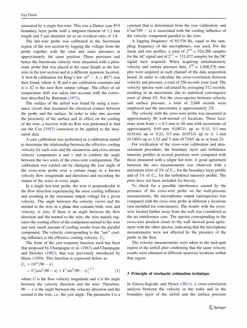
Figure 11a illustrates the time evolution of the y distri-

bution of the linear pressure sources qL that have been

normalised by Ue2/d*2. It has been calculated from the

stochastically estimated or ‘‘quasi-instantaneous’’ velocity

field. It can be observed that negative pressure peaks

coincide with negative pressure sources and positive peaks

are associated with positive pressure sources. The sources

seem to be distributed across the boundary layer

(d & 3.8d*) and there seems to be good coincidence

between the negative pressure sources and the location of

the strong clockwise vortices observed in the flow structure

of Fig. 8. The positive pressure sources appear upstream

and downstream of these vortices, occupying the same

region of the boundary layer as the negative sources. This

scenario confirms that these dominant clockwise vortices

are responsible for the pressure generation in this particular

case. The term qv0/qx from qL is very strong in the region

near the cores of the main vortices and switches between

negative and positive values creating the negative and

positive pressure sources illustrated in Fig. 11a. The

strength of qv0/qx decreases away from the vortex cores,

however, near the wall, the values of the sources associated

with the wall-pressure generation are still very high. This is

due to the term du/dy from qL, i.e., the mean velocity

gradient, that increases substantially near the wall.

On account of the 1/r decay present in the integral

solution to the Poisson equation, the source term has been

weighted as such and the results are presented in Fig. 11b.

The results from Fig. 11b seem to indicate that from the

point of view of the pressure, the strongest sources are near

the wall, although since the pressure is the result of the

integration over the flow volume, weaker sources that

extend over larger volumes may be equally important as

stronger, more localised sources (Daoud 2004). Hence, it

can be concluded that in the present case, the wall-pressure

sources are distributed across a significant part of the

boundary layer.

5 Conclusions

The complex mechanisms present in the generation of

surface pressure fluctuations by a separated laminar

boundary layer convecting past an airfoil have been inves-

tigated by performing simultaneous measurements of the

surface pressure fluctuations and of the velocity field in the

boundary layer and wake of a NACA0012 airfoil, especially

in the region close to the trailing edge. These detailed

measurements have provided further understanding about

0 20 40 60 80 100 120-5

0

5

τ Ue/δ*

p’/p

rms

0

1

2

3

4

5y/

δ*

-0.2

0

0.2

qLδ*2/U

e2

(a)

-0.2

0

0.2

0 20 40 60 80 100 120

τ Ue/δ*

qL/r δ*3/U

e2

-5

0

5

p’/p

rms

0

1

2

3

4

5

y/δ*

(b)

Fig. 11 Surface pressure time series p0 at x/C = 0.97 and pseudo-

instantaneous linear pressure source, qL, at x/C = 0.98 (5 mm

upstream of the TE). a Contours of qL and b contours of qL weighted,

taking into account the distance to the point of observation of the

pressure

Exp Fluids

123

the flow structures responsible for the wall-pressure gen-

eration. These flow structures comprise the sources of the

wall-pressure field, which are closely related to the sources

of the so-called airfoil self-noise. Improving the under-

standing between the velocity field and the surface pressure

fluctuations is also very important for the flow-induced

vibration problems found in ship hulls or submarine peri-

scopes for example.

The stochastic estimation technique presented in this

paper provided a picture of the ‘‘quasi-instantaneous’’

(velocity vectors) flow structures convecting past the

location of a cross-wire and revealed information about the

variability and evolution of the sources of the wall-pressure

generation. From the stochastic estimation technique, due

to the dominance of the large-scale vortices from the sep-

arated shear layer, the pseudo-instantaneous linear pressure

sources (qL ¼ �2 dudy

ov0

ox) were found to be distributed across

the boundary layer.

Acknowledgments This work was funded by the UK Department of

Trade and Industry under the MSTTAR DARP programme. The

MSTTAR DARP was supported by Rolls-Royce plc and BAE Sys-

tems. The authors are grateful for fruitful discussions with Ahmed

Naguib and his students Mohamed Daoud and Laura Hudy from

Michigan State University and with Charles Tinney from University

of Poitiers (currently at the University of Texas at Austin) and

Lawrence Ukeiley from Florida State University. Special thanks for

their support to Phil Joseph, Neil Sandham, Tze Pei Chong and

Richard Sandberg from the University of Southampton and John

Coupland and Philip Woods from Rolls-Royce and BAE Systems,

respectively. The authors wish to thank Gavin Ross for his out-

standing technical help with the airfoil model instrumentation and the

experimental facility. Ana Garcia-Sagrado also gratefully acknowl-

edges the financial support from the Zonta International Amelia

Earhart Fellowship.

References

Adrian R (1977) On the role of conditional averages in turbulence

theory. In: Proceedings of the 4th biennal symposium on

turbulence in liquids. Princeton, NJ

Adrian R (1979) Conditional eddies in isotropic turbulence. Phys

Fluids 22:2065–2070

Adrian R, Meinhart C, Tomkins C (2000) Vortex organisation in the

outer region of the turbulent boundary layer. J Fluid Mech

422:1–54

Agarwal NK, Simpson RL (1989) A new technique for obtaining the

turbulent pressure spectrum from the surface pressure spectrum.

J Sound Vib 135((2):346–350

Bearman PW (1971) Correction for the effect of ambient temperature

drift on Hotwire measurements in incompressible flow. DISA Inf

11:25–30

Blake W (1970) Turbulent boundary-layer wall-pressure fluctuations

on smooth and rough walls. J Fluid Mech 44:637–660

Blake WK (1975) A statistical description of pressure and velocity

fields at the trailing edges of a flat structure. Technical report,

David W. Taylor Naval Ship R&D Center Report No. 4241

Blake W (1986) Mechanics of flow induced sound and vibration,

Volume I (General Concepts and Elementary Sources) and

Volume II (Complex Flow-Structure Interactions). Applied

Mathematics and Mechanics Volume 17-I and Volume 17-II

Bonnet J, Delville J, Glauser M, Antonia R, Bisset D, Cole D, Fiedler

H, Garem J, Hilberg D, Jeong J, Kevlahan N, Ukeiley L,

Vincendeau E (1998) Collaborative testing of eddy structure

identification methods in free turbulent shear flows. Exp Fluids

25:197

Brooks TF, Hodgson TH (1981) Trailing edge noise prediction from

measured surface pressures. J Sound Vib 78:69–117

Champagne FH, Sleicher CA (1967) Application of multi-point

correlation techniques to aerodynamic flows. Am Inst Aeronaut

Astronaut 28:177–182

Champagne FH, Sleicher CA, Wehrmann OH (1967) Turbulence

measurements with inclined hot-wires. Part. 1 Heat transfer

experiments with inclined hot-wire. J Fluid Mech 28:153–175

Cox RN (1957) Wall neighborhood measurements in turbulent

boundary layers using a hot-wire anemometer. A.R.C. Report

19191

Daoud MI (2004) Stochastic estimation of the flow structure

downstream of a separating/reattaching flow region using wall-

pressure array measurements, Ph.D. thesis, Michigan State

University

Ewing D, Citriniti J (1997) Examination of a LSE/POD complemen-

tary technique using single and multi-time information in the

axisymmetric shear layer. In: Sorensen, Hopfinger, Aubry (eds)

Proceedings of the IUTAM symposium on simulation and

identification of organised structures in flows. Kluwer, Lyngby,

pp 375–384

Fahy FJ, Gardonio P (2007) Sound and structural vibration: radiation,

transmission and response. Elsevier, Amsterdam

Fiedler HE (1988) Coherent structures in turbulent flows. Prog

Aerospace Sci 25:231–269

Garcia-Sagrado A, Hynes T (2011) Wall pressure sources near an

airfoil trailing edge under separated laminar boundary layers.

AIAA J (submitted)

Goody MC (1999) An experimental investigation of pressure

fluctuations in three-dimensional turbulent boundary layers,

Ph.D. thesis, Virginia Polytechnic Institute and State University,

Blacksburg, VA

Gravante SP, Naguib AM, Wark CE, Nagib HM (1998) Character-

isation of the pressure fluctuations under a fully developed

turbulent boundary layer. AIAA J 36(10)

Guezennec Y (1989) Stochastic estimation of coherent structures in

turbulent boundary layers. Phys Fluids A 1:1054–1060

Helal HM, Casarella MJ, Farabee T (1989) An application of noise

cancellation techniques to the measurement of wall pressure

fluctuations in a wind tunnel. Am Soc Mech Eng 22:14–22

Hinze JO (1959) Turbulence: an introduction to its mechanism and

theory. McGraw-Hill Series in Mechanical Engineering, New York

Hudy L, Naguib A, Humphreys W (2003) Wall-pressure-array

measurements beneath a separating/reattahing flow region. Phys

Fluids 15:706–717

Mish PF (2001) Mean loading and turbulence scale effects on the

surface pressure fluctuations occurring on a NACA0015 airfoil

immersed in grid generated turbulence, Master thesis, Virginia

Polytechnic Institute and State University, Blacksburg, VA

Naguib AM, Gravante SP, Wark C (1996) Extraction of turbulent

wall-pressure time-series using an optimal filtering scheme. Exp

Fluids 22:14–22

Naguib A, Wark C, Juckenhfel O (2001) Stochastic estimation and

flow sources associated with surface pressure events in a

turbulent boundary layer. Phys Fluids 13:2611–2626

Roger M, Moreau S (2004) Broadband self-noise from loaded fan

blades. AIAA J 42(3)

Rozenberg Y, Roger M, Moreau S (2006) Effect of blade design at

equal loading on broadband noise. In: Proceedings of the 12th

Exp Fluids

123

AIAA/CEAS aeroacoustics conference, Cambridge, Massachu-

setts. AIAA Paper No. 2006-2563

Rozenberg Y, Roger M, Guedel A, Moreau S (2007) Rotating blade

self noise: experimental validation of analytical models. In:

Proceedings of the 13th AIAA/CEAS aeroacoustics conference,

Rome. AIAA Paper No. 2007-3709

Taylor G (1938) The spectrum of turbulence. Proc R Soc Lond Ser A

164:476–490

Tinney C, Coiffet F, Delville J, Hall A, Jordan P, Glauser M (2006)

On spectral linear stochastic estimation. Exp Fluids 41:763–775

Vernet A, Kopp GA, Ferre JA, Giralt F (1999) Three-dimensional

structure and momentum transfer in a turbulent cylinder wake.

J Fluid Mech 394:303–337

Wark C, Naguib A, Ojeda W, Juckehoefel O (1998) On the

relationship between the wall pressure and velocity field in a

turbulent boundary layer. Am Inst Aeronaut Astronaut, AIAA

Paper No. 98-2642

Yu JC, Joshi MC (1979) On sound radiation from the trailing edge of

an isolated airfoil in a uniform flow. AIAA Paper 79-0603

Exp Fluids

123