Stochastic Analytics in the Database - IBM · Stochastic Analytics in the Database Chris Jermaine*...
66
1 August, 2010 Stochastic Analytics in the Database Chris Jermaine* Ravi Jampani Luis Perez Mingxi Wu Fei Xu U. Florida Gainesville *Rice University Peter J. Haas Kevin Beyer Vuk Ercegovac Bo Shekita IBM Almaden Research Ctr.
Transcript of Stochastic Analytics in the Database - IBM · Stochastic Analytics in the Database Chris Jermaine*...

1August, 2010
Stochastic Analyticsin the Database
Chris Jermaine* Ravi Jampani
Luis PerezMingxi Wu
Fei Xu
U. Florida Gainesville*Rice University
Peter J. HaasKevin Beyer
Vuk ErcegovacBo Shekita
IBM Almaden Research Ctr.

2August, 2010
Outline
• Motivation via examples• MCDB: Monte Carlo Database System• MC3: MCDB + map-reduce• Future directions

3August, 2010
Problem Setting
• Large data sets• Missing or uncertain data• Stochastic models used to “guess” values
– Model gives probability distribution on data values• Want to run BI queries over guessed values• Want to assess uncertainty in query answers
– Risk assessment– Decisionmaking
??
?

4August, 2010
Ex. 1: Portfolio Values
CustID OptionID NumShares …
23 50
……
…
…
John Smith
…
OptionID InitVal … StrikeP
23 $4.00
OVal
…
…
…
$2.35 ?
… …
Customer EuroCallOptions
SELECT SUM (c.NumShares * o.Val)FROM Customer c, EuroCallOptions oWHERE c.OptionID = o.OptionID
AND c.CustType = ‘Institutional’
Sample fromNormal dist’n
( )+ Δ = + Δ + Δ( ) ( ) ( ) ( ) ( ) jV t t V t rV t t a V t V t tZ
Simulation approximation (Euler formula):
( ) ( )= + = −final OVal max ( ) ,0dV rV dt a V V dW V t S
Modified Black-Scholes model for European call option:
Option valueone month from now
(exercise date)

5August, 2010
Ex. 2: Pricing Decisions
• Can analyze arbitrary dynamic customer segments when determining effect of price increase
• Similar approach for web-click behavior (EBay, Websphere portal)• Issues: Complex model, huge number of dynamic parameters
Data for allcustomers pr
ice
demand
Global demanddistribution (prior)
Data for onecustomer pr
ice
demand
Individual demanddistribution (posterior)
CustIDUnitPrice
Order Amount
J. Smith $10.20 500
… … …
Bayes Theorem
6August, 2010
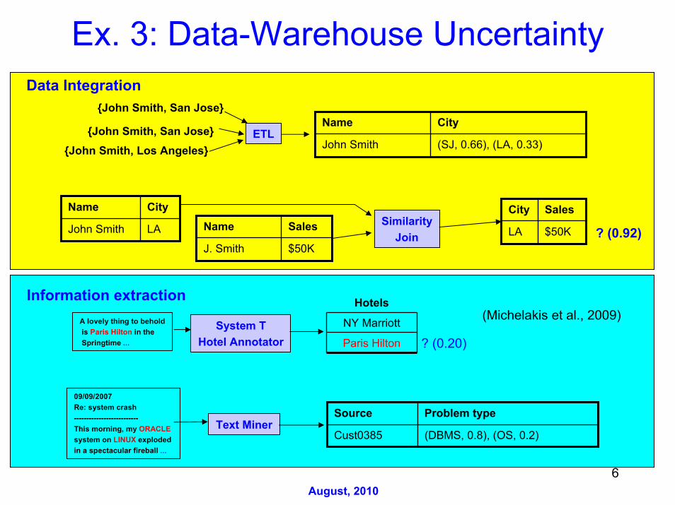
Ex. 3: Data-Warehouse Uncertainty
ETL{John Smith, San Jose}{John Smith, Los Angeles}
Name City
John Smith (SJ, 0.66), (LA, 0.33)
Text MinerSource Problem type
Cust0385 (DBMS, 0.8), (OS, 0.2)
09/09/2007Re: system crash--------------------------This morning, my ORACLEsystem on LINUX explodedin a spectacular fireball …
Name City
John Smith LA Name Sales
J. Smith $50K
SimilarityJoin
City Sales
LA $50K ? (0.92)
Data Integration
Information extraction Hotels
NY Marriott
Paris Hilton
A lovely thing to beholdis Paris Hilton in theSpringtime …
System THotel Annotator ? (0.20)
{John Smith, San Jose}
(Michelakis et al., 2009)

7August, 2010
Risk Due to Data Uncertainty
• Ex: Value of assets (for financial reporting, compliance, business-process monitoring)
SELECT SUM (s.amount)FROM SALES s, CUST cWHERE s.ID = c.ID
AND c.city = ‘Los Angeles’
prob
abili
tyTotal LA sales
5%VaR
expectedanswer
• Ex: ERP– # OS experts needed for help desk– Based on (uncertain) extracted text data from last year– Provide principled safety factor
Query-resultdistribution

8August, 2010
Traditional Workflow
Analyst (PhD)Develops model
Model
Datareduction
Model fitting Model application& querying
Arena, R, Matlab,…
Model
• Data extraction slow and bug-prone• Only coarse-grained modeling• No encapsulation for user
• Hard to re-link model results to DB• Hard to deal with data updates• Sensitivity, what-if analysis are hard
Goal: Integrate model with Database Model
Arena, R, Matlab,…

9August, 2010
Prior Work
• MauveDB (Deshpande & Madden 06)– Continuous deterministic models only
• Probabilistic databases(Trio, MayBMS, ORION, MystiQ, K-relations, et al.)– For data-warehouse uncertainty– Hard-wired, limited uncertainty model (deterministic skeleton)– Limited queries (top-k)– Complexity issues– Independence assumptions– What-if analysis is hard

10August, 2010
Outline
• Motivation • MCDB: Monte Carlo Database System• MC3
• Future directions

11August, 2010
The MCDB System
Q(D) = Select SUM(sales)
AS t_sales
SchemaVG Functions
Parameter Tables
Random DB = D
Monte CarloGenerator
Monte Carlo
Estimator
i.i.d. samples from possible-worlds
dist’n
E [ t_sales ]Var [ t_sales ]q.01 [ t_sales ]
HistogramError bounds
Inference
ˆˆ
ˆ
Q(d1)Q(d2)
:Q(dn)
i.i.d. samples from query-result
dist’n
d1
d2
dn
...
Q
Q
Q

12August, 2010
MCDB Example
Q: SELECT SUM(Amount) FROM SALES
AS t_sales
CID Region
102 NewEngland
226 Midwest
CUST_ATTR
CID Shape
102 1.2
226 0.7
AMT_SHAPE
Region Scale
NewEngland 7.0
Midwest 2.1
AMT_SCALE
CID Amount
102 $120.00
226 $60.00
Gamma(shape, scale)
CID Amount
CID Shape Scale
102 1.2 7.0
2.1226 0.7
SALES
CID Amount
102 $80.00
226 $90.00
CID Amount
102 $80.00
226 $130.00
d1 d2
VG function
d3
Q(d1) = $180 Q(d2) = $170 Q(d3) = $210
E[t_sales] = $186.67 STD[t_sales] = $20.82ˆ ˆ

13August, 2010
Advantages of MCDB
• Flexible and extensible uncertainty model– Can capture extended relational models (Trio, MayBMS, Mystiq,…)– Can capture huge range of stochastic models
• Can bring complex stochastic models to data (no extraction needed)
• Encapsulates complexity– Once expert has written VG function, naïve user can run queries
• Can handle arbitrary SQL queries
• What-if analysis, sensitivity analysis, data updates are easy

14August, 2010
VG FunctionsValue WeightSan Jose 0.66
San Francisco 0.34 DiscreteChoice()parameter table
Pseudorandom #seed
• Used to generate instances of values in random tables– Parameter tables are standard relational tables (can index, etc.)– Library of standard functions: DiscreteChoice, Normal, Poisson, …– Can define custom functions (similar to UDFs)
ValueSan Jose
output table(instance)

15August, 2010
Pseudorandom Number Generators (PRNG)
• Needed by VG function– E.g., to generate “random” sales values
• Produces a deterministic sequence of seeds– Appears random– Cycles around
• Typical PRNG recurrence:– Si+1 = M * Si mod m– Seed S = vector of k unsigned integers– M is a matrix
• Transform seeds to desired random samples• Cycle usually “split” into disjoint segments
– Skip factor• Keeping only initial seed, S0, is sufficient to
regenerate sequence
Sn-1S0 S2
S1
PRNG Cycle of Seeds
. ..

16August, 2010
VG Functions and Correlation
ID1 ID2 Cov1
1
2
1 1.23
2 0.17
2 2.45
MDNormal()
Pseudorandom #seed
ID Mean1
2
3.68
4.75
V1 V21.21 2.13
ID Val1
2
1.21
2.13
or
Correlatedcolumns
Correlatedrows

17August, 2010
Schema Syntax: ExampleCREATE TABLE RAND_CUST (CID, GENDER, MONEY, LIVES_IN) ASFOR EACH d in CUSTWITH MONEY AS Gamma((SELECT n.SHAPE FROM MONEY_SHAPE n WHERE n.CID = d.CID),(SELECT sc.SCALE FROM MONEY_SCALE sc WHERE sc.REGION =
d.REGION),(SELECT SHIFT FROM MONEY_SHIFT))WITH LIVES_IN AS DiscreteChoice ((SELECT c.NAME, c.PROBFROM CITIES cWHERE c.REGION = d.REGION)
)SELECT d.CID, d.GENDER, m.VALUE, l.VALUEFROM MONEY m, LIVES_IN l

18August, 2010
Query Processing
• Naïve approach– Repeatedly instantiate DB and run query– Has horrible performance
• MCDB approach– Execute query plan once– Process tuple bundles instead of tuples
• Represents tuple in all simulated possible worlds (MC reps)• Permits a variety of performance optimizations

19August, 2010
Tuple Bundles (4 MC Repetitions)
(Jane, Smith, 20)(Jane, Smith, 21)
--(Jane, Smith, 21)
Tuple bundle
(Jane, Smith, (20,21,x,21), (T,T,F,T), Seed) Representation
(Jane, Smith, (T,T,F,T ), Seed) Compressed representation
isPresent
Basic ideas: (a) Keep bundles in compressed form whenever possible(b) Apply selections early to compressed bundles(c) Amortize I/O, network costs, etc. over multiple reps

20August, 2010
Operations on Tuple Bundles• Seed:
• Split:
• Inference:
(Jane, Smith, --, --) u(Jane, Smith, --, --, Seed)
(Jane, Smith, (20,21,20,21), (T,T,T,T), Seed) u(Jane, Smith, 20, (T,F,T,F), Seed),(Jane, Smith, 21, (F,T,F,T), Seed)
(Jane, Smith, (20,21,20,21), (T,T,T,T), Seed) u(Jane, Smith, 20, 0.5), Also: Aggregate
(Jane, Smith, 21, 0.5)

21August, 2010
Standard Operations• Select (FNAME = ‘Jane’ AND AGE = 20)
• Join (equijoin on Department #)
(Jane, Smith, (20,21,20,21), (F,T,T,T), Seed)(John, Jones, (32,31,20,30), (T,T,F,T), Seed)(Jane, Jones, (21,23,22,22), (T,T,T,T), Seed) u
(Jane, Smith, (20,21,20,21), (F,F,T,F), Seed)
(Smith, (D1,D2,D2,D1), (F,T,T,T), Seed1) (Jones, (D1,D2,D2,D2), (T,T,F,T), Seed2) u
(Smith, D2, Jones, D2, (F,T,F,F), Seed1, Seed2)
Uses SPLIT+
sort-merge

22August, 2010
Estimation and Inference
MCDB inference operator
TotSales Frac
20K
…
0.324
…
OutputTable
WITH Stats(Mu, Var) AS (SELECT SUM(Val1*Frac),
SUM(Val*Val1*Frac) - SUM(Val1*Frac)*SUM(Val1*Frac)
FROM OutputTable)SELECT Mu AS Mean, SQRT(Var) AS Stdev,
1.96*SQRT(Var)/SQRT(1000) AS CIHWFROM Stats
Distincttuple values
Frac. replications where
value appears(vs bit vector)
WITH CumDistFn(TotSales, Cum, PrevCum) AS (SELECT TotSales,
SUM(Frac) OVER (ORDER BY TotSalesROWS BETWEEN UNBOUNDED PRECEDING AND CURRENT ROW),
SUM(Frac) OVER (ORDER BY TotSalesROWS BETWEEN UNBOUNDED PRECEDING AND 1 PRECEDING)
FROM OutputTable)SELECT Val FROM CumDistFnWHERE Cum >= 0.5 AND PrevCum < 0.5SQL queries

23August, 2010
Experimental Queries
• Q1: Next year’s revenue gain from Japanese products– Assuming current trends hold– Each order duplicated Poisson # of times– Poisson mean = (this year)/(last year) for customer
• Q2: Order Delays– From placement to delivery– Fitted Gamma distribution for each delay type (for each part)
• Q3: What if we had used cheapest supplier?– TPC-H only has current prices– Prior prices generated by backwards random walk with drift
• Q4: Change in profits with 5% price increase– Bayesian model of customer demand– Based on all customers orders at current price

24August, 2010
Results 1 (1000 Reps*)
8.2 8.25 8.3 8.35 8.4 8.45 8.5
x 109
0
20
40
60
Revenue change
Fre
qu
ency
Q1
200 250 300 350 400 4500
20
40
60
80
Days until completion
Fre
qu
ency
Q2
1.3375 1.338 1.3385 1.339 1.3395 1.34 1.3405 1.341
x 1010
0
10
20
30
40
Total supplier cost
Fre
qu
ency
Q3
−8.842 −8.84 −8.838−8.836−8.834−8.832 −8.83 −8.828
x 1010
0
20
40
60
80Q4
Additional profits
Fre
qu
ency
Long tail inDelivery times
*Q3 histogram based on 350 reps

25August, 2010
Results 2: Execution Times (Min)Query 1 rep 10 reps 100 reps 1000 repsQ1 25 25 25 28Q2 36 35 36 36Q3 37 42 87 222*Q4 42 45 60 214
*Based on 350 reps
• Much faster than naïve method in all cases
vs 25000, 36000

26August, 2010
Outline
• Motivation• MCDB• MC3: MCDB + map-reduce• Future directions

27August, 2010
Motivation
• Exploit massive parallelism of MCDB computations– Extend domain of applicability
• Faster path to market?– Forward-looking architecture
• Handle semi-structured, nested data– E.g., web-click example: Petabytes of log file data
• Local expertise/interest in map-reduce– Learning experience for interesting analytical problem– MCDB computations often CPU-intensive– Ease of prototyping

28August, 2010
Technical Issues
• How to represent bundles?• How to specify map-reduce jobs?• How to parallelize?• How to seed tuple bundles?

29August, 2010
A Cluster-Computing Infrastructure
Jaql
Map-Reduce
HDFS
High-level query language for
semi-structured JSON data
Distributed File System
Parallel batch processing
Hadoop
www.jaql.org//code.google.com/p/jaql
Initial prototype built in a few weeks

30August, 2010
Map-Reduce Overview
PartitionedInput File:
PartitionedOutput File:
M1
M4
M2
M3
R1
R2
[(K, V)]
(K, V)
(Km, [Vm])
[Vr]
[(Kr, Vr)]
• Programmer focus:– Map: (K,V) → [(Km,Vm)]– Reduce:
(Km, [Vm]) → [(Kr,Vr)]
• System provides:– Parallelism– Sorting– Synchronization– Fault tolerance– Resource allocationOn commodity hardware
[(Km, Vm)]
(NULL, “This is a line of text”)
[(“This”,1),…,(“text”,1)]
(“This”, [1,1,…,1])
[(“This”,528),(“is”,2000),…]
Ex: parallel word counting

31August, 2010
MCDB Example
Q: SELECT SUM(Amount) FROM SALES
AS t_sales
CID Region
102 NewEngland
226 Midwest
CUST_ATTR
CID Shape
102 1.2
226 0.7
AMT_SHAPE
Region Scale
NewEngland 7.0
Midwest 2.1
AMT_SCALE
CID Amount
102 $120.00
226 $60.00
Gamma(shape, scale)
CID Amount
CID Shape Scale
102 1.2 7.0
2.1226 0.7
SALES
CID Amount
102 $80.00
226 $90.00
CID Amount
102 $80.00
226 $130.00
d1 d2
VG function
d3
Q(d1) = $180 Q(d2) = $170 Q(d3) = $210
E[t_sales] = $186.67 STD[t_sales] = $20.82ˆ ˆ

32August, 2010
JSON and MC3
[{cid: 102, region: NewEngland}, …]
[{cid: 102, shape: 1.2, scale: 7.0}, …]
[{cid: 102, shape: 1.2, scale: 7.0, seed: 306576301}, …]
[{cid: 102, shape: 1.2, scale: 7.0, amount: { seed: 306576301,
samples: [$120.30, $65.00, … ] },isPresent: [T, T, … ]
}, …]
Join + Project
Seed
Instantiate

33August, 2010
JAQL and MC3: Example1 $cust = READ(hdfs(‘cust_attr’));$shape = READ(hdfs(‘amt_shape’));
$scale = READ(hdfs(‘amt_scale’));
2 JOIN $shape, $cust, $scaleWHERE $shape.cid == $cust.cid
AND $cust.region == $scale.regionINTO {$shape, $scale}
//Seed3 → TRANSFORM { $.*, seed: GetSeed() }//Instantiate: generate array of 1000 samples
4 → TRANSFORM GenAmounts($.seed, $.shape, $.scale, 1000)// Sum all sales tuple bundles
6 → GROUP INTO ArraySum($)// Compute the distribution
7 → TRANSFORM Distribution($)8 → WRITE(hdfs(‘result’));

34August, 2010
Example of a Query Plan
Read ‘CUST_ATTR’
Read ‘AMT_SHAPE’
Join (cid)
Join (region)
1. Final ArraySum2. Distribution3. Write ‘result’
Map
Read
1. GetSeed2. GenAmounts3. Partial ArraySum
Reduce
Read ‘AMT_SCALE’
Job 3
Job 2
Job 1

35August, 2010
Parallelism Schemes
• Inter-tuple parallelism– Partition tuple bundles among nodes– Natural fit with Map-Reduce– Good when many bundles or cheap VG functions
• Intra-tuple parallelism– Split up tuple bundles
• Break Monte Carlo replications into chunks– Apply inter-tuple parallelism methods to chunks– Good when few tuples with
• Expensive VG functions and/or• Many MC replications
Tuple 1: (r1,…,r1000)
Tuple 2: (r1,…,r1000)…
Tuple 1: (r1,…,r500)
Tuple 1: (r501,…,r1000)
…
Tuple 2: (r1,…,r500)
Tuple 2: (r501,…,r1000)

36August, 2010
Distributed Seeding
• Must avoid overlapping seed sequences• Maximize parallelization (tuples on different processors)• Minimize seed size stored in each tuple
…Tuple 1 Tuple 2 Tuple n

37August, 2010
Skip-Ahead Method• Well512a generator: period = 2512
• Assume inter-tuple parallelism (for simplicity)• Assume that we know (or have good upper bound for)
– # of bundles seeded per node (= b)– # of seeds per VG function call (= c)– # MC reps (= n)
Tuple j at node i:
Tuple j at node i: Makem = b × i + j
skips of length c × nto get to starting point
{cid: 102, shape: 1.2, scale: 7.0}
{cid: 102, shape: 1.2, scale: 7.0, seed: [i, j] }Actually, only O(log m)
skips needed:pre-computeSkip factors
Seeding
Instantiation

38August, 2010
Scale-up Results:Inter-Tuple Parallelism
• Implemented two nontrivial queries from MCDB paper– Jaql: Map-Reduce plan = original MCDB plan– Good scalability with inter-tuple parallelism
0 1 2 3 4 5 6 7 8 9 10600
850
1100
1350
1600
1850
Number of Servers
Run
ning
Tim
e (s
)
Q4Q1

39August, 2010
Speed-up Results:Intra-Tuple Parallelism
• Implemented two call-option queries (Euro and Asian)– Euro option: expensive VG function, good speed-up– Asian option: cheap VG function, speed-up curve flattens
• Sequential merging of chunks starts to dominate– Moral: choose appropriate parallelization scheme
0 4 8 16 24 32 40 48 56 64 72 80048
16
24
32
40
48
56
64
72
80
Number of Cores
Spe
edup
Ideal SpeedupEuropean OptionAsian Option

40August, 2010
Outline
• Motivation• MCDB• MC3
• Future directions

41August, 2010
An End-to-End ERP Scenario
Requirements formechanics and parts
(safety margin)
Automobile problem reports (text)
My S-Class slipped out of gear …
ProbIE
My S-Class slipped out of gear …
Tire Problem (0.2)
Transmission problem (0.9)
ProbabilisticBI querying
SELECT COUNT(REPORTS)
WHERE P_TYPE = ‘transmission’

42August, 2010
Future Directions• Tail Sampling
– Extreme-quantile (VAR) estimation and more– “Gibbs cloner” approach
• Performance– Query optimization
• E.g., push down inference & instantiation,choose parallelization scheme
• Improve JAQL rewriter (MC3 aware)?• Re-use of partial results, multi-query optimizations?
– Sequential and/or adaptive simulation? (MC3)– Combine with exact methods? Sampling?– Indexing, etc.
• Functionality– User-defined precision– Semi- and unstructured data– Robust, full-featured re-implementation (underway)
• Possible Applications– Automotive ERP– Health records

43August, 2010
Related Projects• RAQA: Resolution-aware query
answering for Business Intelligence[Sismanis et al., ICDE09]
– Uncertainty due to entity resolution– OLAP querying (roll-up, drill-down)– Bounds on query answers– Implemented via SQL queries– Conservative approach
• ProbIE: Probabilistic info extraction[Michelakis et al., SIGMOD09]
– For rule-based IE system (e.g., SystemT)– Provides confidence #’s for base/derived
annotations– Based on “rule history”, lower-level results– MaxEnt-based learning approach
• Other Monte Carlo/Statistics analysis in Hadoop (XAP)
– Operational risk calculations– RICARDO: synthesis of R and Hadoop
[Das et al., SIGMOD10]– Recommender systems
City State Strict range Status
San Francisco CA [$30,$230] guaranteed
San Jose CA [$70,$200] non-guaranteed
State Strict range Status
CA [$230,$230] guaranteed
Sum(Sales) group by City,State
Sum(Sales) group by State
Annotator rulesLabeled training dataRule features
probIE
Annotation probability
Statisticalmodel
Text
Annotator
Annotation +Rule history
Learning phase
Deploymentphase

44August, 2010
Further Details:
www.almaden.ibm.com/cs/people/[email protected]
Thank You!
• MCDB: SIGMOD 2008• MC3: SIGMOD 2009• ProbIE: SIGMOD 2009• MCDB-R: VLDB 2010

45August, 2010
Backup Slides

46August, 2010
Clinic-Capacity Risk
Medical data for allcustomers
Pharmacy data for allcustomers
Stochasticdosage model
Cox hazard-ratedisease model
CustID Time period Resource needed
Jane Smith June-Sept ?
… …
Clinic-resourcedemand model

47August, 2010
Individual Click Behavior (EBay)
• Can analyze arbitrary dynamic customer segments when determining effect of changing EBay pages
Click data for allEBay customers
Global Markov modeldistribution (Dirichelet prior)
Data for onecustomer
Individual Markov modeldistribution (posterior)
x32
p1
p4
p3
p2
x13
x14x34
x24
y32
p1
p4
p3
p2
y13
y14y34
y24

48August, 2010
Logistics Under Uncertainty• Retailer: ship from warehouses to outlets today or tomorrow?• Deterministic tables
• Random tables
• Queries:
• Issues:– Complicated statistical models for purchase quantity (how to integrate in DB?)– Uncertainty (random tables) depend dynamically on huge number of parameters
ITEM_ID QUANTITY
curtains 50
… …
ShipmentITEM_ID QUANTITY
curtains 20
… …
In_StockITEM_ID Price
curtains $120
… …
Current_Price
CUST_ID ITEM_ID QUANTITY
Smith curtains ?
… …
Sales_W_ShipCUST_ID ITEM_ID QUANTITY
Smith curtains ?
… …
Sales_WO_Ship
SELECT SUM (c.price * s.quantity)FROM SALES_W_SHIP s, CUR_PRICE cWHERE c.ITEM_ID = s.ITEM_ID
SELECT SUM (c.price * s.quantity)FROM SALES_WO_SHIP s, CUR_PRICE cWHERE c.ITEM_ID = s.ITEM_ID

49August, 2010
Data Uncertainty - Continued
{JohnSmith, age 42} Privacy FilterName Age
John Smith Between 40 and 50
Event Time
Buffer overflow 10/17/2007:18:20:02System Monitor
t
f(t)
Anonymization
Measurement Uncertainty
Sensor_ID Temp (F)
S23 78.32Sensor
t
f(t)
78.32

50August, 2010
VG Function Implementation• C++ class with four
public methods– Initialize: set up data
structures, seed RNG– TakeParams: read in
“parameter vector”– OutputVals: return
random value(s) for possible world
• Return NULL when done
– Finalize: clean up
If newRep:newRep = falseuniform = myRanDGen()probSum = i = 0while (uniform >= probSum)
i++probSum += L[i].wt / totWeight
return L[i].valElsenewRep = truereturn NULL
OutputVals methodFor DiscreteChoice()

51August, 2010
Schema Syntax: Example 1
• Goal: generate random customer table– MONEY, LIVES_IN are uncertain attributes– MONEY has Gamma dist’n
• shift, shape, scale parameters– Use DiscreteChoice for LIVES_IN value– Customers are mutually independent, given region
• Parameter table schemas– CUST (CID, GENDER, REGION)– CITIES (NAME, REGION, PROB)
• Probabilities sum to 1 in each region– MONEY_SHIFT (SHIFT)– MONEY_SCALE (REGION, SCALE)– MONEY_SHAPE (CID, SHAPE)
Normalizedstorage
1 row, 1 column

52August, 2010
Schema Syntax: Example 2
CREATE TABLE RAND_CUST (CID, GENDER, MONEY, LIVES_IN) ASFOR EACH d in CUSTWITH MLI AS MyJointDistribution(…)SELECT d.CID, d.GENDER, MLI.V1, MLI.V2FROM MLI
MLI has 1 row, 2 columns
• Suppose MONEY and LIVES_IN are correlated

53August, 2010
Schema Syntax: Example 3• Correlated sensors
– Sensors in same “sensor group” are correlated (multivariate normal)• Parameter table schemas
– S_PARAMS (ID, LAT, LONG, GID)– MEANS (ID, MEAN)– COVARS (ID1, ID2, COV)
CREATE TABLE SENSORS (ID, LAT, LONG, TEMP) ASFOR EACH g in (SELECT DISTINCT GID FROM S_PARAMS)WITH TEMP AS MDNormal (
(SELECT m.ID, m.MEAN FROM MEANS m S_PARAMS ssWHERE m.ID = ss.ID AND ss.GID = g.GID),(SELECT c.ID1, c.ID2, c.COV FROM COVARS c, S_PARAMS ssWHERE c.ID1 = ss.ID AND ss.GID = g.GID)
)SELECT s.ID, s.LAT, s.LONG, t.VALUEFROM S_PARAMS s, TEMP t WHERE s.ID = t.ID

54August, 2010
Instantiate Operation
“inner” input pipes“outer”input pipe
B1 B2 B3
pipe fork
πVGAtts seed{ }∪
πInAtts1 seed{ }∪ πInAtts2 seed{ }∪ πInAtts3 seed{ }∪πOutAtts seed{ }∪
Qin,1 Qin,2 Qin,3Qout
outputpipe M ergeseed
VG Function
Sortseed
M ergeseed
For-eachclause
VG functionargs

55August, 2010
Q4 Details• Effect on profits of 5% price increase
– Want more accuracy than usual aggregated demand functions• E.g, exploit detailed point-of-sale data
– For each part• Fit “prior” demand-function distribution to all customers (MLE)• Determine “posterior” distribution for each cust. (Bayes Thm)• Generate random demand for each customer at new price• Use rejection algorithm to sample from posterior
P
Q{Gamma(a,b)
Gamma(c,d)

56August, 2010
Multi-PRNG Method• When # of seeds per VG function call is unknown• When skip-ahead for huge PRNG is hard to implement• Collisions possible, but probability < 10-17
Seeding at node i Instantiation of tuple j
G1
G2
bundle j
bundle j
G3
G4
16 ints
4 ints
6 ints
(small)
s0
(huge)
Shared by All nodes
6 ints x [# bundlesat nodes 0 to (i-1)]
(medium)
(medium)

57August, 2010
Nested-Data Experiments
• TPC-H schema is used• Two different ways to nest data
– Nest lineitem table under orders table– Nest lineitem table under partsupp table
• Modified version of Q4 from MCDB paper– Compare MC3 execution time to flat scheme– First nesting scheme: running time is slower– Second nesting scheme: running time is faster
• Only uncertain “leaf attributes” are supported

58August, 2010
Probabilistic Information Extraction in a Rule-Based System
Annotator Candidate-Generation Rules Rule PrecisionPerson
PersonPhone HighHigh
Medium
HighHighLow
PhoneNumber HighMedium
Low
P1: <Salutation><CapitalizedWord><CapitalizedWord> P2: <First Name Dictionary><Last Name Dictionary>P3: <CapitalizedWord><CapitalizedWord>
Ph1: <PhoneClue><\d{3}-\d{3}-\d{4}>Ph2: <\d{3}-\d{3}-\d{4}>Ph3: <\d{5}
PP1: <Person><“can be reached at”><PhoneNumber>PP2: <“call”><Person><0-2 tokens><PhoneNumber>PP3: [<Person><PhoneNumber>]sentence
+ Consolidation ruleConsolidate(“Joe Smith”, “Mr. Joe Smith”) = “Mr. Joe Smith”
Derivedannotator
Baseannotator
Baseannotator
Motivation: System T Hand-crafted rules for specific domain:

59August, 2010
Annotations
Goal: Attach probabilities to annotations in a principled, scalable manner

60August, 2010
Quantifying this uncertainty is critical as
• Extracted facts can then be queried using probabilistic databases
• Confidence numbers can be used by information integration and search applications
• It helps in improving the recall of annotators!!

61August, 2010
Our approach
• Propose a probabilistic framework for handling uncertainty in rule-based IE– Each annotation is associated with a confidence
• the probability that the annotation is correct– Probability is obtained by augmenting each annotator with
a statistical model• Design considerations
– Applicable to grammar and declarative rule-based IE systems
– Scale to annotators with a large number of (correlated) rules
– Support incremental improvements in accuracy of probability estimates
• as rules, data, or constraints are added

62August, 2010
Rule Histories and Features
Please call Heather Choate at
span
P1 P2 P3r = ( 0, 1 , 1)
P1: <Salutation><CapitalizedWord><CapitalizedWord> P2: <First Name Dictionary><Last Name Dictionary>P3: <CapitalizedWord><CapitalizedWord>
Rule history
• Rule features– Qualitative correlations and anti-correlations– Ex: “Rules P1 and P2 tend to occur together”
• Rule history

63August, 2010
ProbIE Framework(Base Annotator)
Annotator rulesLabeled training data
Rule featuresprobIE
Annotation probability
Statisticalmodel
Text AnnotatorConsolidated span +
Rule history
Learning phase
Extraction (deployment) phase

64August, 2010
Probability Model of Uncertainty• Binary random variables associated with text and annotator
– A(s) = 1 iff span s is actually a Person– K(s) = 1 iff span s is annotated as a Person by consolidator– R(s) = (R1(s),R2(s),…,Rk(s)) is stochastic rule history on span s
• Ri(s) = 1 iff ith rule holds at least once on span s
• Annotation probability:
q(r) = P(A(s) = 1 | R(s) = r, K(s) = 1)
• Indirect approach (estimate a prob dist’n rather than many small probs)– Estimate
p0(r) = P(R(s) = r | A(s) = 0, K(s) = 1)
p1(r) = P(R(s) = r | A(s) = 1, K(s) = 1) u
= P(A(s) = 1 | K(s) = 1)
– is easy to estimate empirically– Serious data-sparsity problem for p0 and p1: 2k possible histories, little training data– Solution: Fit a parametric model
1
1 0
p (r)q(r)p (r) (1 )p (r)
π=π + − π

65August, 2010
A Parametric Model• Parametric exponential model for p1 (model for p0 is similar):
– Recall: p1(r) = P(R(s) = r | A(s) = 1, K(s) = 1) with R(s) = (R1(s),…,Rk(s))– From features to constraints
P(R3(s) = 1 | A(s) = 1, K(s) = 1) = a3 (one marginal constraint per rule)
P(R2(s) = 1 and R7(s) = 1 | A(s) = 1, K(s) = 1) = a2,7 (important correlations)
where constants a3, a2,7, etc. computed from training data– Approximate p1 by “simplest” (maximum entropy) distribution satisfying constraints– Equivalent to maximum-likelihood fit of parameter vector for exponential distribution
– Use improved iterative scaling (IIS) to fit from training data
• Model-decomposition methods for IIS scalability to many rules and constraints
• Augment training data to handle constraints with 0 right-hand side
• Methodology extends to derived annotators such as PersonPhone
{ }1 c cc C
1p (r; ) exp f (r)Z( ) ∈
θ = θθ ∑ fc = Indicator function
for constraint c

66August, 2010
Some Experimental Results(Pay-As-You-Go)
Person annotator(No inter-rule constraints)
Person annotator(4 inter-rule constraints)