STM103 Spring 2009 - Harvard University ‐ Introduction to Stata ‐2009 1 STM103 Spring 2009...

Norris ‐ Introduction to Stata ‐2009 1

STM103 Spring 2009

INTRODUCTION TO STATA

1. DOWNLOADING DATA: ...................................................................................................................... 2 Assignment 1 preparation .......................................................................................................................... 3 Select variables ........................................................................................................................................... 3

2. STARTING A STATA SESSION .............................................................................................................. 4 Opening, Saving, and Closing the data file ................................................................................................. 5 Keeping a log record of a Stata Session ...................................................................................................... 5 Using Operators .......................................................................................................................................... 5

3. WORKING WITH DATA ....................................................................................................................... 6 To see what your selected variables contain: ............................................................................................ 6 To look at the % distribution in categorical variables ................................................................................ 7 To look at a table combining two categorical variables ............................................................................. 7 Creating and Changing Values of Variables ................................................................................................ 8 Labeling Variables and Values .................................................................................................................... 9 Using Functions .......................................................................................................................................... 9 Deleting Variables and Observations ......................................................................................................... 9 list ......................................................................................................................................................... 10 Analysis of continuous (scale) variables ................................................................................................... 10 Correlations .............................................................................................................................................. 10 Estimating Linear Models (OLS and 2‐Stage Least Squares) ..................................................................... 11 Estimating Non‐Linear Models (Logit and Probit) .................................................................................... 11 logit ......................................................................................................................................................... 11 probit ........................................................................................................................................................ 12

4. MAKING GRAPHS ............................................................................................................................. 12 Histogram ................................................................................................................................................. 12 Scatterplot ................................................................................................................................................ 12 Bar graphs ................................................................................................................................................. 13 Printing your graph ................................................................................................................................... 13

5. UTILITIES ......................................................................................................................................... 13 Viewing the Data ...................................................................................................................................... 13 Creating and Submitting a Do File ............................................................................................................ 13

6. CONVERTING DATA FILES (EXCEL TO STATA) .................................................................................... 14 This provides a brief introduction to using Stata for the QoG dataset analysis. Stata is available on all of the computers in the Kennedy School’s computer lab. If you have a home computer you may want to purchase a copy of Stata from the CMO. Stata is available for Windows98, Windows 2000, Windows ME, Windows XP, Windows NT, Macintosh, and UNIX operating systems. The Stata User’s Guide is also available from the CMO.

The commands outlined below assume that you are using Stata for Windows. Throughout this text, anything appearing in Bold font is a Stata command, whereas anything in red italics is a variable name which you should change for your specific analysis. Menu commands are indicated as, e.g., File | Open, to indicate that you first go to the File menu and then choose the Open option. The Blue Courier is the type of output you should generate. As a shortcut, you can also just copy and paste any of the command lines here directly into your Stata Command window then run.


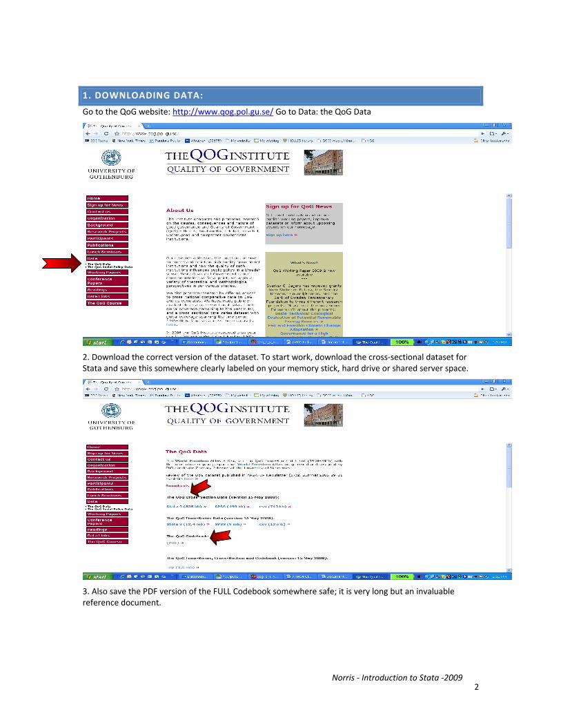
1. DOWNLOADING DATA:

Go to the QoG website: http://www.qog.pol.gu.se/ Go to Data: the QoG Data

2. Download the correct version of the dataset. To start work, download the cross‐sectional dataset for Stata and save this somewhere clearly labeled on your memory stick, hard drive or shared server space.

3. Also save the PDF version of the FULL Codebook somewhere safe; it is very long but an invaluable reference document.


ASSIGNMENT 1 PREPARATION

The aim is to write a professional report assessing and comparing the problems of democratic governance reform in one world region. Pick your region:

Latin America and the Caribbean,

Africa,

Asia,

Central and Eastern Europe,

Middle‐East

Western Europe

Think about the key problems of democratic governance in the region. From your experience and your reading, what are the priorities for agencies? Can you rank them? Focus on the most important 2‐3 issues in the first instance. Then look carefully at the shared dataset codebook. Start by selecting 3‐4 indicators which relate to the problems you have decided to focus upon. The shared class dataset provides the following indicators, along with many others:

1. Freedom House index of political rights and civil liberties 2. Polity IV Project Democracy and Autocracy scales 3. Cheibub and Gandhi Democracy‐Autocracy classification 4. Vanhanen Democracy Index 5. World Values Survey/Global Barometers Attitudinal surveys 6. Kaufmann/Kray World Bank Institute Good governance indicators 7. Transparency International Corruption index

SELECT VARIABLES

You can use the whole dataset without doing anything further but there are a LOT of variables in the dataset. To simplify your life and make it less confusing, for this exercise you will find it easier to identify a sub‐set of key variables from the What It Is list which you want to use.

You can always go back to select more variables at a later stage (none are deleted) but first work out which variables to put into your subset i.e. what is important as indicators of democratic governance for your region. Note in Stata it matters whether variable names are in capitals or not.

Select the first ones listed below and pick about 5‐10 to add. Write down details in the list below so that you have this handy. Look in the full codebook for more details about the construction and meaning of each.

Name Brief description Type

cname Country name Nominal

ht_region Global region: 10 categories Nominal

chga_regime Cheibub and Ghandi: Type of democratic or autocratic regime Nominal

fh_status Freedom House: classification of states into free, semi‐free and not‐free

Ordinal

p_polity Combined polity score of democracy and autocracy Scale ‐10/+10

fh_cl Freedom House civil liberties Scale 7‐pt

fh_pr Freedom House political rights Scale 7‐pt

wbgi_vae World Bank: Voice and accountability estimate Scale

wbgi_pse World Bank: Political stability estimate Scale

wbgi_gee World Bank: Government effectiveness Scale


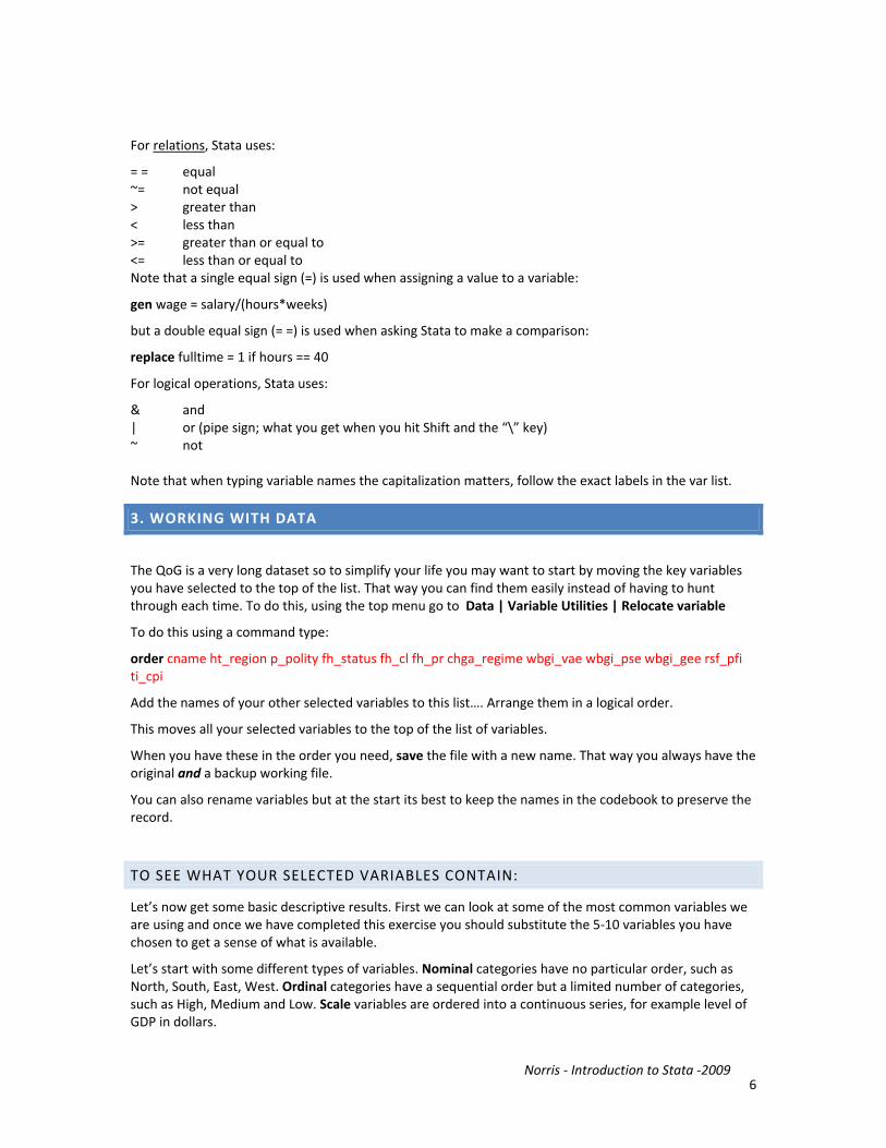
rsf_pfi Reporters without Borders: Press Freedom Index Scale 100‐pts

ti_cpi Transparency International: Corruption Perception Index Scale 100‐pts

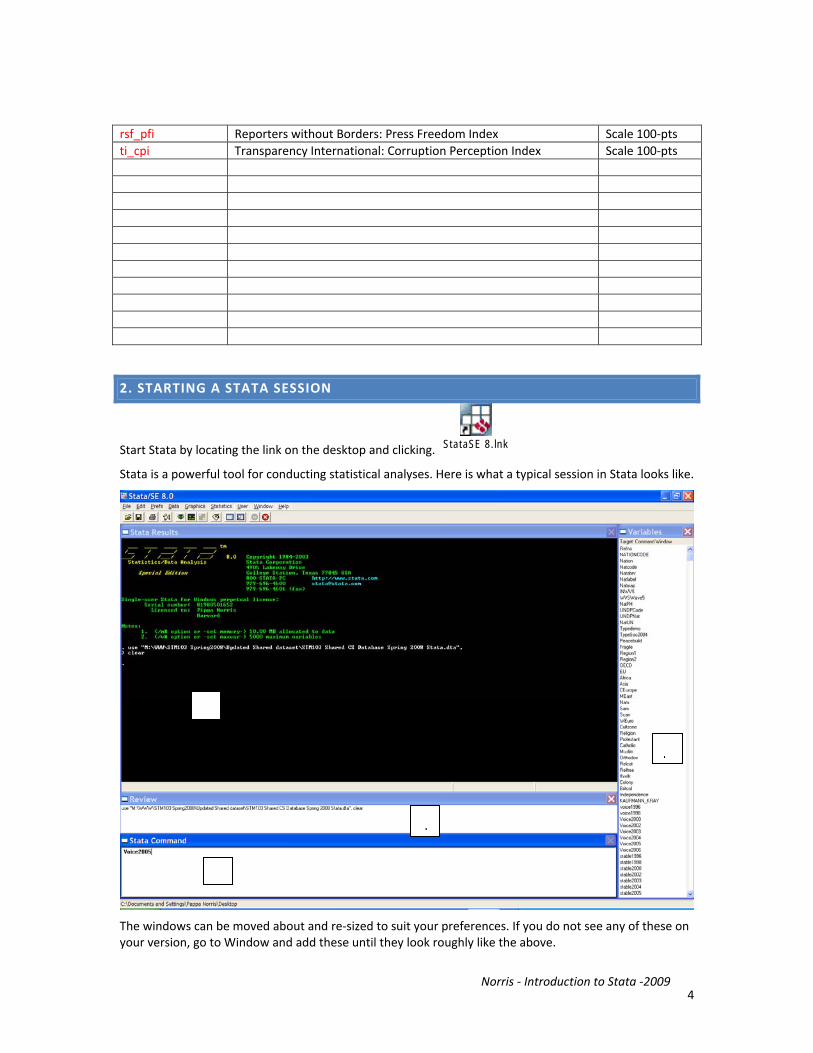
2. STARTING A STATA SESSION

Start Stata by locating the link on the desktop and clicking. StataSE 8.lnk

Stata is a powerful tool for conducting statistical analyses. Here is what a typical session in Stata looks like.

The windows can be moved about and re‐sized to suit your preferences. If you do not see any of these on your version, go to Window and add these until they look roughly like the above.

b

d


a. Here the Results window lists the outcome.

b. The Variables window, on the left, lists the names of all the variables included in the shared dataset.

c. You can enter commands in two ways. To start learning the program, you can use the drop down menus, similar to those common in Microsoft programs. This is useful for beginners. Once you become more familiar with the program, you will want to type in commands directly, to save time, using the Command window at the bottom center of the screen. A command tells Stata what to do – e.g, to open a file, to run a regression, to calculate a mean of a variable, etc.

d. The Review window shows a list of all the commands you have already run. (Here, it shows that I have opened a data file.) If you click on a previously‐run command in the Review window, it will appear in the Command window and you can edit it or run it again.

OPENING, SAVING, AND CLOSING THE DATA FILE

You will then need to open the data file you have saved. You may need to boost the memory allocated.

Set memory 80000

File | Open

File| Save As

It is also always useful to have a backup copy of your data. This way, no matter what you do to change or recode the variables, you always have a copy of the older version. It is also useful practice to save your data file at the end of each session under a new sequential version (eg STM103_2, STM103_3, so that you have the old and newest file in case you need to revert back.

File | Exit

Whenever you finish, to exit Stata.

KEEPING A LOG RECORD OF A STATA SESSION

File| log

To save a file (“log”) of your results, you will need to create a log file. Stata gives you two choices of file formats for your log file, .log (text file) and .smcl (formatted log file). The .smcl files will look nicer when printed. You should never ever cut and paste your Stata output directly into your report; always simplify, clean and transfer in a professional and clean format.

To start a log file interactively, choose File | Log | Begin, select the directory you want to save the log file in, and give it a name (such as job1). Alternately, you can click on the fourth icon from the left on the icon bar, which looks like a scroll.

File |Log | Close

USING OPERATORS

Stata uses the following arithmetic operators:

+ add ‐ subtract * multiply / divide ^ raise to the power


For relations, Stata uses:

= = equal ~= not equal > greater than < less than >= greater than or equal to <= less than or equal to Note that a single equal sign (=) is used when assigning a value to a variable:

gen wage = salary/(hours*weeks)

but a double equal sign (= =) is used when asking Stata to make a comparison:

replace fulltime = 1 if hours == 40

For logical operations, Stata uses:

& and | or (pipe sign; what you get when you hit Shift and the “\” key) ~ not Note that when typing variable names the capitalization matters, follow the exact labels in the var list.

3. WORKING WITH DATA

The QoG is a very long dataset so to simplify your life you may want to start by moving the key variables you have selected to the top of the list. That way you can find them easily instead of having to hunt through each time. To do this, using the top menu go to Data | Variable Utilities | Relocate variable

To do this using a command type:

order cname ht_region p_polity fh_status fh_cl fh_pr chga_regime wbgi_vae wbgi_pse wbgi_gee rsf_pfi ti_cpi

Add the names of your other selected variables to this list…. Arrange them in a logical order.

This moves all your selected variables to the top of the list of variables.

When you have these in the order you need, save the file with a new name. That way you always have the original and a backup working file.

You can also rename variables but at the start its best to keep the names in the codebook to preserve the record.

TO SEE WHAT YOUR SELECTED VARIABLES CONTAIN:

Let’s now get some basic descriptive results. First we can look at some of the most common variables we are using and once we have completed this exercise you should substitute the 5‐10 variables you have chosen to get a sense of what is available.

Let’s start with some different types of variables. Nominal categories have no particular order, such as North, South, East, West. Ordinal categories have a sequential order but a limited number of categories, such as High, Medium and Low. Scale variables are ordered into a continuous series, for example level of GDP in dollars.


First let’s summarize your selected variables. Type:

sum ht_region p_polity fh_cl fh_pr

Variable | Obs Mean Std. Dev. Min Max

-------------+--------------------------------------------------------

ht_region | 192 4.526042 2.644633 1 10

p_polity | 160 1 14.45487 -77 10

fh_cl | 192 3.385417 1.821166 1 7

-------------+--------------------------------------------------------

fh_pr | 192 3.364583 2.156785 1 7

chga_regime | 189 .3968254 .4905386 0 1

This is very useful for looking at your selected variables to see what they are like, whether nominal, ordinal or scale (continuous). E.g. chga_regime is a binary 2‐ category variable. Try this for a couple of your variables and add notes to your selected vars on page 2.

summarize can be abbreviated to sum. You can also look at more detail. eg

sum ht_region, detail

You can do the same just for one selected region

sum p_polity if ht_region == 1, detail

TO LOOK AT THE % DISTRIBUTION IN CATEGORICAL VARIABLES

For categorical variables, try the following which generates some simple frequencies ie look at the number of countries (Freq) and the percent column.

. tab1 ht_region

The Region of the Country | Freq. Percent Cum.

----------------------------------------+-----------------------------------

1. Eastern Europe and post Soviet Union | 27 14.06 14.06

2. Latin America | 20 10.42 24.48

3. North Africa & the Middle East | 20 10.42 34.90

4. Sub-Saharan Africa | 48 25.00 59.90

5. Western Europe and North America | 27 14.06 73.96

6. East Asia | 6 3.13 77.08

7. South-East Asia | 11 5.73 82.81

8. South Asia | 8 4.17 86.98

9. The Pacific | 12 6.25 93.23

10. The Caribbean | 13 6.77 100.00

----------------------------------------+-----------------------------------

Total | 192 100.00

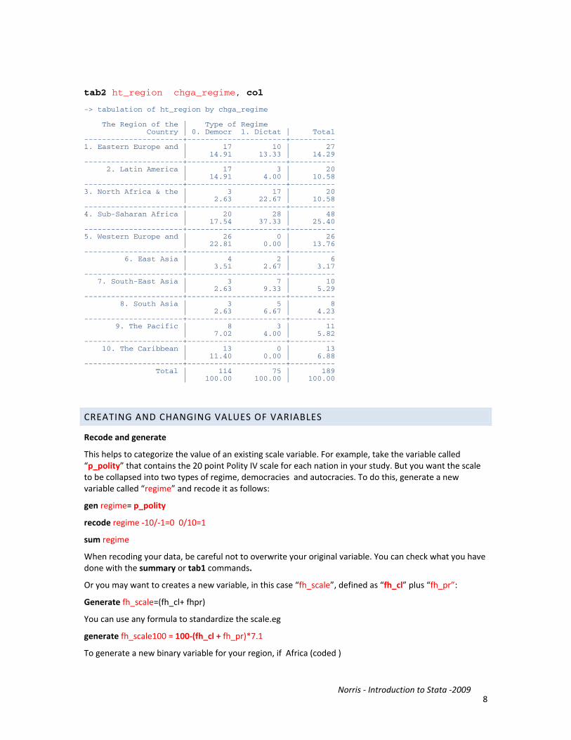
TO LOOK AT A TABLE COMBINING TWO CATEGORICAL VARIABLES


tab2 ht_region chga_regime, col -> tabulation of ht_region by chga_regime The Region of the | Type of Regime Country | 0. Democr 1. Dictat | Total ----------------------+----------------------+---------- 1. Eastern Europe and | 17 10 | 27 | 14.91 13.33 | 14.29 ----------------------+----------------------+---------- 2. Latin America | 17 3 | 20 | 14.91 4.00 | 10.58 ----------------------+----------------------+---------- 3. North Africa & the | 3 17 | 20 | 2.63 22.67 | 10.58 ----------------------+----------------------+---------- 4. Sub-Saharan Africa | 20 28 | 48 | 17.54 37.33 | 25.40 ----------------------+----------------------+---------- 5. Western Europe and | 26 0 | 26 | 22.81 0.00 | 13.76 ----------------------+----------------------+---------- 6. East Asia | 4 2 | 6 | 3.51 2.67 | 3.17 ----------------------+----------------------+---------- 7. South-East Asia | 3 7 | 10 | 2.63 9.33 | 5.29 ----------------------+----------------------+---------- 8. South Asia | 3 5 | 8 | 2.63 6.67 | 4.23 ----------------------+----------------------+---------- 9. The Pacific | 8 3 | 11 | 7.02 4.00 | 5.82 ----------------------+----------------------+---------- 10. The Caribbean | 13 0 | 13 | 11.40 0.00 | 6.88 ----------------------+----------------------+---------- Total | 114 75 | 189 | 100.00 100.00 | 100.00

CREATING AND CHANGING VALUES OF VARIABLES

Recode and generate

This helps to categorize the value of an existing scale variable. For example, take the variable called “p_polity” that contains the 20 point Polity IV scale for each nation in your study. But you want the scale to be collapsed into two types of regime, democracies and autocracies. To do this, generate a new variable called “regime” and recode it as follows:

gen regime= p_polity

recode regime ‐10/‐1=0 0/10=1

sum regime

When recoding your data, be careful not to overwrite your original variable. You can check what you have done with the summary or tab1 commands.

Or you may want to creates a new variable, in this case “fh_scale”, defined as “fh_cl” plus “fh_pr”:

Generate fh_scale=(fh_cl+ fhpr)

You can use any formula to standardize the scale.eg

generate fh_scale100 = 100‐(fh_cl + fh_pr)*7.1

To generate a new binary variable for your region, if Africa (coded )


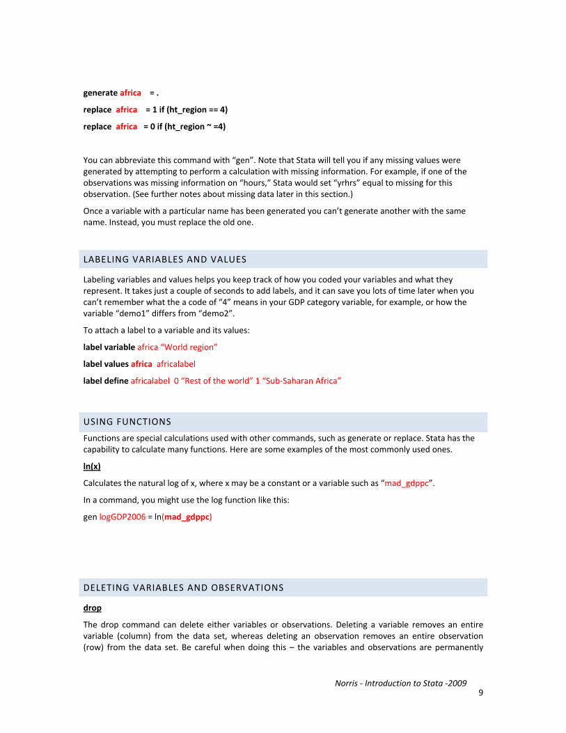
generate africa = .

replace africa = 1 if (ht_region == 4)

replace africa = 0 if (ht_region ~ =4)

You can abbreviate this command with “gen”. Note that Stata will tell you if any missing values were generated by attempting to perform a calculation with missing information. For example, if one of the observations was missing information on “hours,” Stata would set “yrhrs” equal to missing for this observation. (See further notes about missing data later in this section.)

Once a variable with a particular name has been generated you can’t generate another with the same name. Instead, you must replace the old one.

LABELING VARIABLES AND VALUES

Labeling variables and values helps you keep track of how you coded your variables and what they represent. It takes just a couple of seconds to add labels, and it can save you lots of time later when you can’t remember what the a code of “4” means in your GDP category variable, for example, or how the variable “demo1” differs from “demo2”.

To attach a label to a variable and its values:

label variable africa “World region”

label values africa africalabel

label define africalabel 0 “Rest of the world” 1 “Sub‐Saharan Africa”

USING FUNCTIONS

Functions are special calculations used with other commands, such as generate or replace. Stata has the capability to calculate many functions. Here are some examples of the most commonly used ones.

ln(x)

Calculates the natural log of x, where x may be a constant or a variable such as “mad_gdppc”.

In a command, you might use the log function like this:

gen logGDP2006 = ln(mad_gdppc)

DELETING VARIABLES AND OBSERVATIONS

drop

The drop command can delete either variables or observations. Deleting a variable removes an entire variable (column) from the data set, whereas deleting an observation removes an entire observation (row) from the data set. Be careful when doing this – the variables and observations are permanently


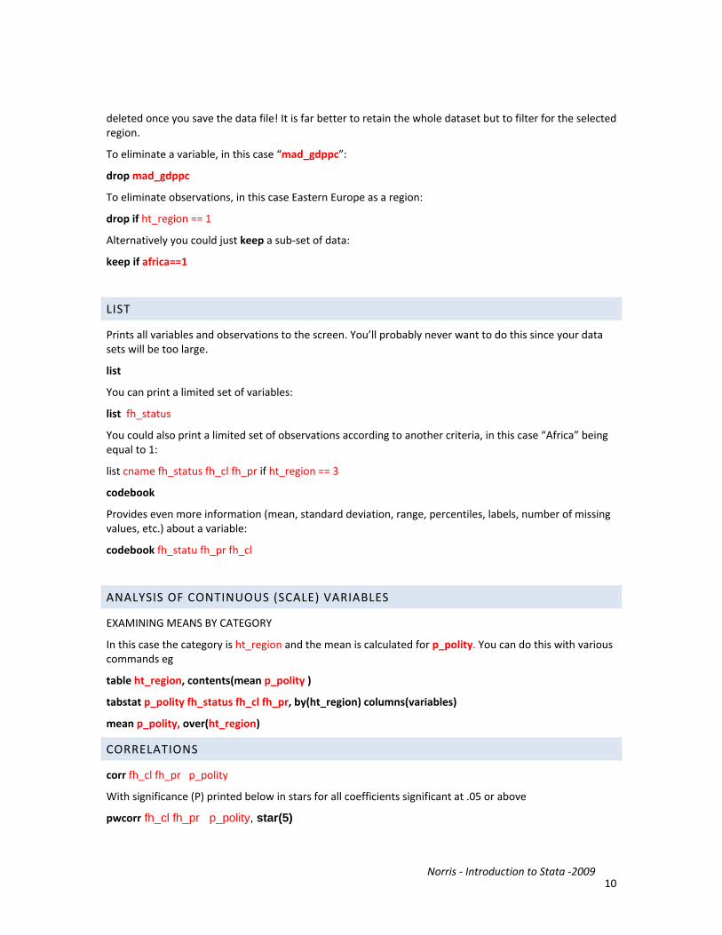
deleted once you save the data file! It is far better to retain the whole dataset but to filter for the selected region.

To eliminate a variable, in this case “mad_gdppc”:

drop mad_gdppc

To eliminate observations, in this case Eastern Europe as a region:

drop if ht_region == 1

Alternatively you could just keep a sub‐set of data:

keep if africa==1

LIST

Prints all variables and observations to the screen. You’ll probably never want to do this since your data sets will be too large.

list

You can print a limited set of variables:

list fh_status

You could also print a limited set of observations according to another criteria, in this case “Africa” being equal to 1:

list cname fh_status fh_cl fh_pr if ht_region == 3

codebook

Provides even more information (mean, standard deviation, range, percentiles, labels, number of missing values, etc.) about a variable:

codebook fh_statu fh_pr fh_cl

ANALYSIS OF CONTINUOUS (SCALE) VARIABLES

EXAMINING MEANS BY CATEGORY

In this case the category is ht_region and the mean is calculated for p_polity. You can do this with various commands eg

table ht_region, contents(mean p_polity )

tabstat p_polity fh_status fh_cl fh_pr, by(ht_region) columns(variables)

mean p_polity, over(ht_region)

CORRELATIONS

corr fh_cl fh_pr p_polity

With significance (P) printed below in stars for all coefficients significant at .05 or above

pwcorr fh_cl fh_pr p_polity, star(5)


ESTIMATING LINEAR MODELS (OLS AND 2‐STAGE LEAST SQUARES)

regress

Calculates an ordinary least squares (OLS) regression, in this case for a regression of the dependent “p_polity” on the independents “GDP” and “al_ethnic”. Note that the dependent variable is the first variable listed.

regress p_polity mad_gdppc al_ethnic

If you wish to only include observations with “Africa” equal to 1 in the regression:

regress p_polity mad_gdppc al_ethnic if africa == 1

To run a regression with robust standard errors:

regress Stable2006 GDP2006 Africa, robust

To run two‐stage least squares where “GDP” is endogenous and “z1" is an exogenous instrumental variable:

regress p_polity al_ethnic (mad_gdppc z1)

Note: If you run a regression containing more than 40 variables, Stata will return an error code saying:

matsize too small

To overcome this problem, reset the maximum number of variables Stata will estimate using the matsize command; the number should be greater than or equal to the total number of variables in the regression.

set matsize 150

predict

Calculates the predicted value for each observation using the coefficients from the last regression estimated and saves these as a variable called “yhat”:

predict yhat

To calculate the residual for each observation using the most recently estimated regression model and save these as a variable called “ehat”:

predict ehat, residual

test

Calculates an F‐test of a joint hypothesis concerning the coefficients in the most recently

estimated linear regression model, in this case with the null hypothesis H0: βage = βsex = 0:

test al_ethnic mad_gdppc

ESTIMATING NON‐LINEAR MODELS (LOGIT AND PROBIT)

LOGIT

Estimates a model suitable for a dichotomous dependent variable. In this case, the variable “chga_regime” equals 1 for democracy and 0 for autocracy.

logit chga_regime al_ethnic mad_gdppc


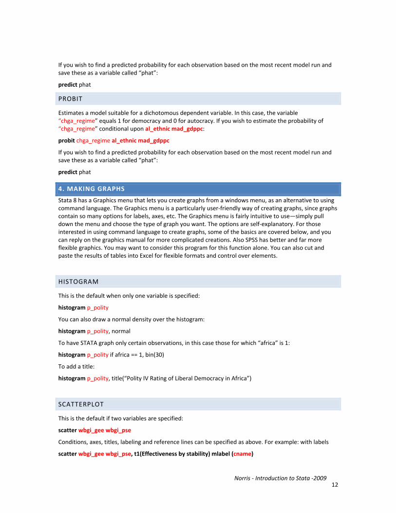
If you wish to find a predicted probability for each observation based on the most recent model run and save these as a variable called “phat”:

predict phat

PROBIT

Estimates a model suitable for a dichotomous dependent variable. In this case, the variable “chga_regime” equals 1 for democracy and 0 for autocracy. If you wish to estimate the probability of “chga_regime” conditional upon al_ethnic mad_gdppc:

probit chga_regime al_ethnic mad_gdppc

If you wish to find a predicted probability for each observation based on the most recent model run and save these as a variable called “phat”:

predict phat

4. MAKING GRAPHS

Stata 8 has a Graphics menu that lets you create graphs from a windows menu, as an alternative to using command language. The Graphics menu is a particularly user‐friendly way of creating graphs, since graphs contain so many options for labels, axes, etc. The Graphics menu is fairly intuitive to use—simply pull down the menu and choose the type of graph you want. The options are self‐explanatory. For those interested in using command language to create graphs, some of the basics are covered below, and you can reply on the graphics manual for more complicated creations. Also SPSS has better and far more flexible graphics. You may want to consider this program for this function alone. You can also cut and paste the results of tables into Excel for flexible formats and control over elements.

HISTOGRAM

This is the default when only one variable is specified:

histogram p_polity

You can also draw a normal density over the histogram:

histogram p_polity, normal

To have STATA graph only certain observations, in this case those for which “africa” is 1:

histogram p_polity if africa == 1, bin(30)

To add a title:

histogram p_polity, title(“Polity IV Rating of Liberal Democracy in Africa”)

SCATTERPLOT

This is the default if two variables are specified:

scatter wbgi_gee wbgi_pse

Conditions, axes, titles, labeling and reference lines can be specified as above. For example: with labels

scatter wbgi_gee wbgi_pse, t1(Effectiveness by stability) mlabel (cname)


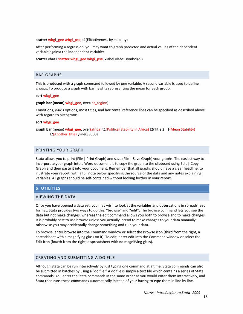
scatter wbgi_gee wbgi_pse, t1(Effectiveness by stability)

After performing a regression, you may want to graph predicted and actual values of the dependent variable against the independent variable:

scatter yhat1 scatter wbgi_gee wbgi_pse, xlabel ylabel symbol(o.)

BAR GRAPHS

This is produced with a graph command followed by one variable. A second variable is used to define groups. To produce a graph with bar heights representing the mean for each group:

sort wbgi_gee

graph bar (mean) wbgi_gee, over(ht_region)

Conditions, y‐axis options, most titles, and horizontal reference lines can be specified as described above with regard to histogram:

sort wbgi_gee

graph bar (mean) wbgi_gee, over(africa) t1(Political Stability in Africa) t2(Title 2) l1(Mean Stability) l2(Another Title) yline(33000)

PRINTING YOUR GRAPH

Stata allows you to print (File | Print Graph) and save (File | Save Graph) your graphs. The easiest way to incorporate your graph into a Word document is to copy the graph to the clipboard using Edit | Copy Graph and then paste it into your document. Remember that all graphs should have a clear headline, to illustrate your report, with a full note below specifying the source of the data and any notes explaining variables. All graphs should be self‐contained without looking further in your report.

5. UTILITIES

VIEWING THE DATA

Once you have opened a data set, you may wish to look at the variables and observations in spreadsheet format. Stata provides two ways to do this, “browse” and “edit”. The browse command lets you see the data but not make changes, whereas the edit command allows you both to browse and to make changes. It is probably best to use browse unless you actually intend to make changes to your data manually; otherwise you may accidentally change something and ruin your data.

To browse, enter browse into the Command window or select the Browse icon (third from the right, a spreadsheet with a magnifying glass on it). To edit, enter edit into the Command window or select the Edit icon (fourth from the right, a spreadsheet with no magnifying glass).

CREATING AND SUBMITTING A DO FILE

Although Stata can be run interactively by just typing one command at a time, Stata commands can also be submitted in batches by using a “do file.” A do file is simply a text file which contains a series of Stata commands. You enter the Stata commands in the same order as you would enter them interactively, and Stata then runs these commands automatically instead of your having to type them in line by line.


For your problem sets, it is strongly recommended that you use do files. Some of the problem sets will require many Stata commands, and it is inevitable that you will need to make changes and run these series of commands a number of times. When you have all of your commands in a single file, it is much easier to go back to that file and make the necessary changes than to have to retype every command.

Creating a Do file

To start creating a do file, click on the Do file editor button (fifth from the right, looks like an envelope with a pencil on it), choose the Do file editor option under the Window menu, or type doedit in the Command window. Note that since a do file is a written list of commands as entered in the Command window, you cannot use the Stata menus within a do file. Instead you need to use the typed (Command window) commands.

6. CONVERTING DATA FILES (EXCEL TO STATA)

The easiest way to convert data files is to use the software program StatTransfer. This program is on the lab computers and allows you to convert your data to or from a variety of different file formats (Stata, SAS Transport, Excel, SPSS, QuatroPro, FoxPro, etc.).

To convert a file from Excel to Stata:

a) Click on the application StatTransfer in the “Data Analysis” folder.

b) Select “Excel Worksheet” for “Input File Type.”

c) Use “Browse” to identify the Excel file you want to convert from. (If the first row of the worksheet contains the variable names, the program will use these as the variable names.)

d) Select “Stata Version 8” as the “Output File Type.” (Since Stata 8.0 is a recent release, it is possible that the version of StatTransfer you’re using will not have Stata Version 8 as an option. If this is the case, save it as a version 7 file; you should still be able to open the file in version 8.)

e) Type in the path and name of the file you wish to create.

f) Begin the conversion by clicking on “Begin Transfer.”

Stata also allows you to read in binary and ASCII files directly. However, in most cases it is easier to first convert your data to a spreadsheet and then convert it to Stata using StatTransfer.


SUMMARY OF SPSS AND STATA COMMANDS

SPSS Command Stata Command(s)

ADD FILES append

AGGREGATE collapse

ANOVA anova

AUTORECODE destring encode

CASESTOVARS reshape wide

COMMENT * /* */

COMPUTE generate replace egen

CORRELATIONS correlate pwcorr

CROSSTABS tabulate tab2

DATA LIST infile infix insheet

DELETE VARIABLES keep drop

DESCRIPTIVES summarize

DISPLAY describe

DOCUMENT notes

DO IF xyzcommand if

DO REPEAT foreach

ECHO display

ERASE erase

EXAMINE tabulate x, summarize(y)

EXECUTE no equivalent

EXPORT no equivalent

FACTOR factor

FILE LABEL label data

FILTER xyzcommand if (___)

FLIP xpose

FORMATS format

FREQUENCIES tabulate

SPSS Command Stata Command(s)

GET FILE use

GET SAS fdause

GRAPH graph

IF generate __ if __

IGRAPH graph

INCLUDE FILE do ___

LIST list

LOGISTIC REGRESSION logistic

LOOP forvalues

MATCH FILES merge

MEANS tabulate __, summarize(__)

MISSING VALUES none

MIXED xtmixed

NOMREG mlogit

PLUM ologit

PROBIT probit

RECODE recode

RECORD TYPE no equivalent

REGRESSION regress

RELIABILITY alpha

RENAME VARIABLES rename

SAMPLE sample

SAVE save

SELECT IF keep if drop if

SORT CASES sort

SPLIT FILE by

SUMMARIZE tabulate ___, summarize(___)

TEMPORARY.SELECT IF (___).

xyzcommand if (___)

T‐TEST ttest

VALUE LABELS

VARIABLE LABELS


Notes:

STM103 Spring 2009 - Harvard University ‐ Introduction to Stata ‐2009 1 STM103 Spring 2009...

Documents

Transcript of STM103 Spring 2009 - Harvard University ‐ Introduction to Stata ‐2009 1 STM103 Spring 2009...