Thanks go to Mumtaz Hussain and Dilip Parajuli for excellent research assistance.1

The limited amount of empirical work on transport costs include Sampson and Yeats (1976) and Pace2

(1979) on OECD countries; Brodsky and Sampson (1979) and Yeats (1976) on Latin America and Asia; and, morerecently, Amjadi and Yeats (1995), Amjadi, Reincke, and Yeats (1996), and UNCTAD (1995) on sub-Saharan Africa. These studies document differences in shipping costs but do not directly estimate the relationship between shipping costsand manufactured exports or economic growth.

Steven RadeletJeffrey SachsJanuary 1, 1998

Shipping Costs, Manufactured Exports, and Economic Growth1

In the Wealth of Nations, Adam Smith put great stress on the relationship betweengeographic location and international trade. Smith observed that a more extensive division oflabor was likely to develop first along sea coasts and navigable rivers, where transport costs wereespecially low:

As by means of water-carriage a more extensive market is opened to every sort of industrythan what land-carriage alone can afford it, so it is upon the sea-coast, and along the banksof navigable rivers, that industry of every kind naturally begins to sub-divide and improveitself, and it is frequently not till a long time after that those improvements extendthemselves to the inland part of the country.

Smith attributed the rapid development of civilizations around the Mediterranean basin to therelative ease of sea-based trade in the region. He saw the shortage of navigable rivers into inlandregions of Africa as a detriment to development on that continent. He also noted the pattern ofrapid development in the New World: “In our North American colonies, the plantations haveconstantly followed either the sea-coast or the banks of navigable rivers, and have scarce anywhere extended themselves to any considerable distance from both.” And so it was in the UnitedStates that the first and most extensive development was along the coast lines; the Mississippi,Ohio, and Hudson River valleys; and the Great Lakes region.

Are Smith’s observations of any relevance today? Are geographical location, especiallyaccess to the sea, still important determinants of a country’s development prospects? Thoughinterest in transport costs has recently risen in the theory of international trade (see, for example, Krugman, 1996), there continues to be almost no empirical work on the role of shipping costs inpatterns of trade and development. In this paper we examine some empirical evidence on2

differences in shipping costs across developing countries, and its impact on manufactured exportsand economic growth. We find that geographical considerations -- specifically access to the seaand distance to major markets -- have a strong impact on shipping costs, which in turn influencesuccess in manufactured exports and long-run economic growth. Countries with lower shipping

Specifically, we exclude SITC (Revision 1) 0-4, 61, 63, 66, 68, and 9.3

The data were prepared by Andrew Mellinger, and are described in Mellinger (1998).4

costs have had faster manufactured export growth and overall economic growth during the pastthirty years than country’s with higher shipping costs. The evidence suggests that high-shippingcost countries will find it more difficult to promote export-led development, even if they reducetariff rates, remove quantitative restrictions, and follow prudent macroeconomic policies. At aminimum, firms in such countries would be forced to pay lower wages to compensate for highertransport costs in order to be able to compete on world markets for manufactures. The requiredoffset in wages might be quite substantial in the usual case for developing countries in whichimported inputs constitute a high proportion of the value of exports. In such sectors, hightransport costs can easily wipe out export profitability even if wage levels were to fall to zero. Asa result, geographically remote countries such as Mongolia, Rwanda, Burundi, Bolivia may notrealistically be able to replicate the East Asian model of rapid growth based on the export oflabor-intensive manufactes.

Casual observation suggests that Smith’s observation of a strong tie between access to thesea and manufactured trade holds true today. Table 1 shows the top 15 developing countryperformers between 1965-90 in terms of annualized growth of non-primary-based manufacturedexports (that is, excluding manufactured exports derived from natural resources, such asdiamonds, plywood, and mineral manufactures ), measured as a percent of GDP. For each year t,3

we calculate (X - X )/GDP , where X is the level of manufactured exports in dollars, and GDPt t-1 t-1

is total GDP in dollars. This measure of export growth, denoted GEXGDP is then averaged overthe years 1965 to 1990. For each country, we also show the share of the population living within100 kilometers of the sea coast, denoted as POP100km based on original calculations at HIIDusing Graphical Information Systems (GIS) data on world population. For our sample of 924

developing countries, the (unweighted) average proportion of the population near the coastline is45 percent. We see that in all except one of the high-export-growth countries, the proportion ofthe population near the coast is much higher than the average. In fact, in most of the top fifteenexporters, nearly the entire population lives within the 100 km radius (often because the economyitself is a small island). Later in the paper we demonstrate that the link between POP100km andGEXGDP during 1965-90 is in fact large and statistically significant, even after controlling forother determinants of export growth. Notice that no landlocked countries are among the topfifteen exporters. Notice as well that almost all of the successful countries are located eitherdirectly on major shipping routes or are close to a major developed-country market (Tokyo,Western Europe, or the United States)

Our focus is on developing countries, which we define as countries with a PPP-adjustedGDP (in 1985 dollars) of $5,000 or less in 1965, using the Penn World Tables Version 5.1. Inany event, most OECD countries, with the exceptions of Australia and New Zealand, are locatedvery close to their major markets -- the other developed countries -- so that transport costs areless of an issue. Our specific concern is with developing countries wishing to initiate labor-intensive export-led growth in manufactures, as in East Asia. Is this development strategydependent on favorable geography? Is it limited to coastal economies close to the major

advanced-country markets?

We begin in the next section by examining some data on shipping costs, and exploringsome factors that might account for differences in these costs across countries. The followingsection examines the relationships between shipping costs, wages, and competitiveness ininternational trade. We then proceed to explore directly the possible relationships betweenshipping costs and long-run economic growth. The final section discusses some otherconsiderations and caveats. We observe, for example, that transport costs are tending to fall overtime, that air shipment provides a viable alternative for at least some production processes, andthat some aspects of shipping costs (customs clearance, ports fees) are very much under thecontrol of policymakers.

Some Determinants of Shipping Costs

Consider the costs of imports. The FOB (free on board) price measures the cost of animported item at the point of shipment by the exporter, specifically as it is loaded on to a carrierfor transport. The CIF (cost-insurance-freight) price measures the cost of the imported item atthe point of entry into the importing country, inclusive of the costs of transport, includinginsurance, handling, and shipping costs, but not including customs charges. The CIF/FOB band,which is our basic measure of shipping costs (SC) is defined as SC = (CIF/FOB) - 1. We measureshipping costs for each country from the point of view of the country’s imports, because that ishow the data are generally available, though obviously shipping costs apply both in the directionof imports and exports. Notice that SC will depend not only on the charges for shipping astandardized type of freight (e.g. a twenty foot equivalent container) but also on the compositionof trade. For very high value added commodities per unit weight (e.g. precious metals) will havevery low CIF/FOB markups. The costs of shipping agricultural exports, similarly, will differdepending on whether they are perishable or dry bulk and the extent to which they have beenprocessed (e.g., groundnuts vs. groundnut oil). Metals and minerals will also differ, depending onthe specific commodity, for example whether the cargo is liquid (e.g., LNG, petroleum) or solid,etc. Thus, countries will differ in their average CIF/FOB ratios not only because of truedifferences in shipping costs for a given composition of goods, but also because of differences inthe commodity mix. We hope that since the import basket of developing countries is morehomogeneous than the export mix, the measure of the CIF/FOB ratio will reveal true differencesin shipping costs rather than commodity mix effects.

In the empirical work below, we use the CIF/FOB ratios published by the IMF (IFSYearbook, 1995), and shown in Table 2. These figures, of course, are not a perfectly accuratemeasure of actual CIF/FOB ratios, since they are in many cases estimated by IMF staff based onincomplete information. For most countries, they show little variance over time, indicating thatIMF staff retain a constant CIF/FOB conversion factor once it is established for a country, andrevise it only infrequently. Nevertheless, these data are relatively consistent and complete, andprovide a good starting point for examining the general costs of international shipping for almostall countries in the world. Surprisingly, more direct shipping cost data — e.g. from transportcompanies — is generally proprietary information and therefore hard to assemble for a largenumber of countries on a systematic basis. We also examined data on shipping costs to the

United States, based on detailed US Department of Commerce data on imports from each countryin the world recorded on both a CIF and FOB basis (as compiled by Feenstra, et al, 1997). Although this data provides very accurate information on shipping costs to the US, it is notindicative of general shipping costs, since the US is not the major market for many countries. Wewere unsuccessful in finding similar import data bases (where data is recorded in both CIF andFOB terms) for Japan or major European countries.

Shipping costs as measured by the CIF/FOB ratios are likely to differ across countries forseveral reasons. First, and most obviously, countries that are located further from major marketsare likely to face higher shipping costs than proximate countries. Second, overland transportcosts tend to be considerably higher than sea freight costs. Thus, for a given distance from mainmarkets, countries with a higher proportion of transit by land will tend to have higher overallshipping costs. Third, there are extra costs to inter-modal transport (e.g. in which freight must beshipped both by land and sea), because of the extra costs of transferring between transport modes. Fourth, shipping costs differ because of differences in the quality of ports administration and/orports infrastructure. Countries with better functioning ports authorities, less red tape for tradersto work through, and more transparent and less corrupt customs clearance are likely to havelower overall shipping costs. Variations in basic port and handling fees can differ widely acrosscountries. Similarly, countries with adequate port capacity, stronger ports infrastructure, andmore sophisticated packaging and loading technologies are likely to have lower shipping costs.

Landlocked countries tend to face enormous cost disadvantages. They must pay the highcosts of overland transport from the neighboring ports. These costs are increased by thebureaucratic and often political costs of crossing at least one additional international border.Infrastructure linking the inland economy with the port may be very poor, since there is a need forcoordinating infrastructure investments in roads, customs houses, and so forth, between thelandlocked country and the port country. The roads linking the landlocked country with the portmay be poorly policed and maintained. Often the coastal economy has no interest in supportingeconomic development in the landlocked country (and may even have an interest in hinderingdevelopment), for geo-strategic reasons. All of these risks probably add to insurance costs, aswell as to basic shipment costs. The only alternative for landlocked countries is to ship by air,which is prohibitively expensive for most goods other than those with the very highest value perunit weight.

The extra shipping costs for six landlocked African countries are shown in Table 3. Thesedata, which are drawn from UNCTAD, show the cost of exporting general cargo from severalAfrican countries to destinations in Northern Europe, East Asia, and North America. The datainclude sea shipment costs for all countries, plus the additional road or rail costs for landlockedcountries. Landlocked countries pay between 25% (Malawi, shipping by rail through Tanzania)and 228% (Burundi, shipping by road through Tanzania) more for similar export shipments toNorthern Europe than their coastal neighbors, even though the overland distances are a smallproportion of the total transport distances. The CIF/FOB data reinforce the conclusions drawnfrom the UNCTAD African data on the extra shipping costs for landlocked countries. For the 97developing countries in our sample, the mean CIF/FOB band in 1965 (the beginning of the timeperiod under review) was 12.9%. For the 80 coastal economies, the average was 11.8%, while

lnSCi ' "0 % "1 lnDISTi % "2 LANDLOCKi % "3 lnGDPi % Li

Note that for the purposes of this analysis, since we are analyzing the extra shipping cost of countries that are5

isolated from major markets, we do not count Austria and Switzerland among the group of landlocked countries. Although they are landlocked, they sit in the midst of the European market, and are thus not economically isolated in thesame sense as other landlocked countries. The cif/fob bands for Austria and Switzerland are 1.8% and 4.1%, amongstthe lowest in the world.

for the 17 fully landlocked countries the average was 17.8%. Thus, the cost of freight andinsurance for landlocked developing countries was, on average, 50% higher than for coastaleconomies.

Results from a simple regression analysis of CIF/FOB ratios are consistent with the basicideas about the underlying determinants of shipping costs, including geography and portefficiency. As our measure of proximity to major world markets, we use the logarithm of the seadistance from each country to nearest major industrial country market. Specifically, we look atthe minimum distance of the country to one of four major ports: Rotterdam, New York, LosAngeles, or Tokyo. (In further work, we will explore taking weighted average distances, basedon the shares of trade with the various markets). The basic specification is:

where SC is the shipping cost in country i (as measured by the CIF/FOB band), DIST is the seai

distance to the nearest major world market, LANDLOCK is a dummy variable (=1) forlandlocked countries, and GDP is PPP-adjusted gross domestic product in 1965 (in 1985 dollars). According to the regression estimates in Table 4, each 10% increase in sea distance is associatedwith a 1.3% increase in shipping costs. For a country with the mean shipping distance (1,900miles) and income levels in our sample, an extra 1,000 miles of sea distance tends to increase theCIF/FOB band by about 0.6 percentage points. In addition, as expected, the results stronglyconfirm that landlocked countries pay more for freight and insurance. At the means for the5

other variables, a landlocked country pays about 5.6 percentage points more for shipping than acoastal economy (i.e., an increase in the CIF/FOB band from 8.9% to 14.5%). This represents anincrease of 63% in freight and insurance costs for landlocked countries, after controlling for theother variables. The difference is statistically significant.

With respect to the quality of ports administration and infrastructure, comparable data onport quality are available for only a small number of countries, so in our base regression, we useas a proxy the log of 1965 GDP per person, measured in constant purchasing power parity prices(Penn World Tables, 1995). Generally speaking, higher income countries are likely to have betterports infrastructure and more efficient ports administration than lower income countries. Theresults show that countries with higher average income in 1965 indeed had significantly lowershipping costs. Each 10% increase in average income is associated with 0.29% lower freightcosts as measured by the CIF/FOB ratio. For a country with the mean shipping distance andincome levels in our sample, an increase in GDP per capita of PPP$500 is associated with andecrease of about 0.5 percentage points in the CIF/FOB band. Note that these three variables

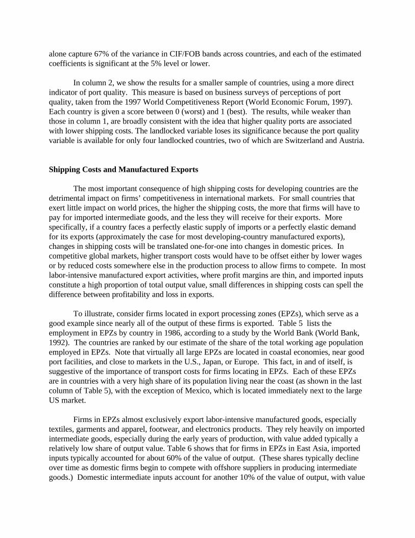
alone capture 67% of the variance in CIF/FOB bands across countries, and each of the estimatedcoefficients is significant at the 5% level or lower.

In column 2, we show the results for a smaller sample of countries, using a more directindicator of port quality. This measure is based on business surveys of perceptions of portquality, taken from the 1997 World Competitiveness Report (World Economic Forum, 1997). Each country is given a score between 0 (worst) and 1 (best). The results, while weaker thanthose in column 1, are broadly consistent with the idea that higher quality ports are associatedwith lower shipping costs. The landlocked variable loses its significance because the port qualityvariable is available for only four landlocked countries, two of which are Switzerland and Austria.

Shipping Costs and Manufactured Exports

The most important consequence of high shipping costs for developing countries are thedetrimental impact on firms’ competitiveness in international markets. For small countries thatexert little impact on world prices, the higher the shipping costs, the more that firms will have topay for imported intermediate goods, and the less they will receive for their exports. Morespecifically, if a country faces a perfectly elastic supply of imports or a perfectly elastic demandfor its exports (approximately the case for most developing-country manufactured exports),changes in shipping costs will be translated one-for-one into changes in domestic prices. Incompetitive global markets, higher transport costs would have to be offset either by lower wagesor by reduced costs somewhere else in the production process to allow firms to compete. In mostlabor-intensive manufactured export activities, where profit margins are thin, and imported inputsconstitute a high proportion of total output value, small differences in shipping costs can spell thedifference between profitability and loss in exports.

To illustrate, consider firms located in export processing zones (EPZs), which serve as agood example since nearly all of the output of these firms is exported. Table 5 lists theemployment in EPZs by country in 1986, according to a study by the World Bank (World Bank,1992). The countries are ranked by our estimate of the share of the total working age populationemployed in EPZs. Note that virtually all large EPZs are located in coastal economies, near goodport facilities, and close to markets in the U.S., Japan, or Europe. This fact, in and of itself, issuggestive of the importance of transport costs for firms locating in EPZs. Each of these EPZsare in countries with a very high share of its population living near the coast (as shown in the lastcolumn of Table 5), with the exception of Mexico, which is located immediately next to the largeUS market.

Firms in EPZs almost exclusively export labor-intensive manufactured goods, especiallytextiles, garments and apparel, footwear, and electronics products. They rely heavily on importedintermediate goods, especially during the early years of production, with value added typically arelatively low share of output value. Table 6 shows that for firms in EPZs in East Asia, importedinputs typically accounted for about 60% of the value of output. (These shares typically declineover time as domestic firms begin to compete with offshore suppliers in producing intermediategoods.) Domestic intermediate inputs account for another 10% of the value of output, with value

added in the EPZ enterprise itself generally around 30%. The precise coefficients vary by sector,as shown by firms in Malaysian EPZs in the early 1980s. Electronics firms imported 78% of thevalue of output, with textile firms importing around 49%. This suggests that the penalty forhigher shipping costs would be especially burdensome for electronics exporters.

A simple numerical example makes the point. Consider a prototypical firm producinglabor intensive manufactured exports from a coastal location, shown in column 1 of Table 7. Following the data described above, CIF imports, domestic inputs, and value added account for60%, 10%, and 30% of the value of FOB output. Suppose that initially this firm faces a CIF/FOBratio of 12% both for imports and exports, and that the demand for its exports and its supply ofimported inputs is perfectly elastic. If this firm were to move to a landlocked country, all of theextra shipping costs would have to be absorbed by lower domestic value added (assuming, forsimplicity, that other domestic intermediate input prices remain unchanged). As shown in column2, an increase in shipping costs of just 6 percentage points, with the CIF/FOB ratio rising to 18%,would wipe off one-third of domestic value added. Assuming that value added is substantiallywage costs, the wage itself would have to be reduced by around two-thirds in order toaccommodate the rise in transport costs! Krugman (1997) has made a similar point concerningthe high elasticity of wages with respect to transport costs in cases where the share of importedinputs in domestic output is high.

Under these circumstances, firms in landlocked countries would not necessarily beprecluded from competing on world markets, but they would almost certainly have to paysubstantially lower wages. For some production processes with a lower import content, such astextiles, shipping costs would have less impact. Zimbabwe, for example, has had some success inmanufacturing textiles for export to markets in Southern Africa. By contrast, for productionprocesses with a high import content, such as electronics, shipping costs can reduce potentialvalue added dramatically. Columns 3 and 4 of Table 7 show that for a typical landlocked country(with a CIF/FOB band of 18%), value added in electronics would only be half the value added in acoastal economy. Under these circumstances, a CIF/FOB band of 24% would wipe out all thevalue added in electronics production. Five of the countries listed in Table 2 have a cif factorgreater than 24%, as undoubtedly do many other countries for which data are not available.

Since shipping costs can have such a huge impact on value added and profitability in labor-intensive manufactured exports, it stands to reason that countries with higher freight andinsurance costs would face great difficulty in promoting these activities. Countries with highershipping costs would be less likely to attract foreign investment in export activities, and theirdomestic firms would tend to be less competitive on international markets. To test this idea, weexamined a wide range of variables that might be closely associated with the average annualgrowth rate of non-primary manufactured exports. Since some countries can record a very highgrowth rate when the volume of exports is very small, we again measure the growth ofmanufactured exports relative to GDP in the previous year (as in Table 1). This analysis expandson the earlier results found in Radelet, Sachs, and Lee (1997).

In addition to geography, government policies influence manufactured exports. Low tariffrates, relatively few quotas, and the absence of barriers to foreign exchange transactions (i.e.

A country is considered to be open if it meets minimum criteria on four aspects of trade policy: (i) average6

tariff rates, (ii) extent of imports governed by quotas and licensing, (iii) average export taxes, and (iv) the size of theblack market premium on the exchange rate.

The overall index is itself an average of five indicators of the quality of public institutions, including: (i) the7

perceived efficiency of the government bureaucracy; (ii) the extent of governmental corruption; (iii) efficacy of the ruleof law; (iv) the presence or absence of expropriation risk; and (v) the perceived risk of repudiation of contracts by thegovernment.

currency convertibility on the current account) are all likely to help firms become morecompetitive in international markets. Of particular importance is likely to be low tariff rates forintermediate inputs and raw materials, since, as we have seen, these can account for a high shareof final output. We use the openness measure constructed by Sachs and Warner (1995), which isthe fraction of years between 1965 and 1990 that the country was considered to be open to trade. 6

Similarly, the quality of public-sector institutions and their relationship to the functioning ofmarkets are likely to be important to exporters. To capture these policy dimensions, we use theindex of institutional quality from Knack and Keefer (1995), which is based on data compiled inthe International Country Risk Guide (1995). This index aims to measure the security of7

property and contractual rights, the efficiency of the government's intervention in markets, and theallocation of public goods.

In addition to government policies, economic structure is likely to affect manufacturedexports. We know that export-GDP ratios are lower in larger economies, so we expect theexport growth to GDP ratios similarly to be lower in larger economies. We measure market sizeby the log of the initial level of gross domestic product in 1965. In addition, greater naturalresource abundance is likely to detract from manufactured exports. Countries with abundantnatural resources are less apt to export manufactured products, as strong resource exports tend toappreciate the real exchange rate (the relative price of tradeable to non-tradeable goods), andthereby to reduce the profitability of exports of manufactures (other than resource-basedmanufactures). We measure natural resource abundance by the share of net exports of primaryproducts (exports minus imports) in GDP, a variant of the measure initially used by Sachs andWarner (1995).

Geographical attributes other than those captured by the shipping cost variable may alsoaffect manufactured exports. In particular, we include the ratio of a country’s coastline distance(in km) to its total land area (in km ). Countries with a longer coastline are likely to have more2

ports, have a larger share of the population with relatively easy access to the sea, and have alarger share of economic activity grounded in international trade. In using this variable, we followAdam Smith, who stressed the importance of England’s long coastline for its sea-based trade. “England, on account of the natural fertility of the soil, of the great extent of the sea-coast inproportion to that of the whole country, and of the many navigable rivers which run through it,and afford the conveniency of water carriage to some of the most inland parts of it, is perhaps aswell fitted by nature as any large country in Europe, to be the seat of foreign commerce, ofmanufactures for distant sale, and of all of the improvements which these can occasion.” (Emphasis added). An alternative, and similar measure, is the proportion of the population livingrelatively near the sea. A larger share of the population living near the sea would tend to raise

GEXGDPi ' $0 % $1 OPENi % $2 INSTi % $3 lnGDPi % $4 NRi % $5 COASTi % $6 lnSCi % Ti

the proportion of trade in the economy for any given CIF/FOB shipping costs. As in Table 1, theparticular measure we use is the share of the population living within 100 kilometers of the sea in1995, as calculated by Mellinger, using GIS-based data on the global population.

We examined the relationship between these variables and the annual weighted growthrate of non-primary manufactured exports for 43 developing countries between 1965 and 1990. The basic form of the regression is:

where GEXGDP is the annual average growth of exports as a share of GDP, OPEN is the Sachs-Warner openness index, INIT is institutional quality, NR is net natural resource exports as a shareof GDP, COAST is the ratio of coastline to land area, and SC is shipping costs. In our estimates,we use a base-year (1965) measure of the CIF/FOB ratio, to ensure that any observed linkbetween shipping costs and export growth is a result of the effect of shipping costs on exports,rather than a result of export growth on reduced shipping costs. In the estimates we excludeSingapore, Hong Kong and Korea from the sample since their growth rates were such largeoutliers from the rest of the sample (in addition, data for Taiwan are not available). However, thebasic conclusions hold with even greater force for these countries.

The results are shown in Table 8. Countries with more open trading systems recorded anaverage growth rate for non-primary manufactured exports that was about 0.5 percentage pointsper year higher than for more closed economies, after controlling for other variables. Theestimated coefficient is highly statistically significant and is robust to alternative specifications. The size of the coefficient is relatively large, since it is approximately equal to the average growthrate of non-primary manufactured exports (as a share of GDP) for the sample. Similarly,institutional quality has a strong and positive relationship with exports. Each one point increase inthis index (on a scale of 1-10) is associated with a 0.13 percentage point increase in the dependentvariable. The size of the domestic economy has the expected negative relationship withmanufactured export growth, but the estimated coefficient is not significant at standard levels. Column 3 shows the results when this variable is excluded. Natural resource abundance is alsonegatively correlated with non-primary manufactured exports. Each ten percentage point increasein the share of net primary product exports is associated with a 0.174 percentage point increase inthe export growth rate. Natural-resource-abundant countries, in general, have much lowergrowth in manufactured exports. Of course, there are some exceptions, such as Malaysia, whichrecorded one of the fastest growth rates in the world for non-primary manufactured exportsduring the period.

As expected, geographical attributes strongly influence the growth of manufacturedexports. The longer a country’s coastline relative to its area, the higher is the growth ofmanufactured exports. Using the alternative measure of the share of the population living within100 km of the coast, the results are even stronger. One possible problem with this variable is thatthe causality could run the other way, from exports to coast population, through internal

migration, since the variable is measured in 1995. To control for this possibility, we alsoestimated the relationship with instrumental variables, using the proportion of the land area within100 km of the coast as an instrument for the proportion of the population within 100 km of thecoast. The IV estimate confirms the importance of the coastal share as a cause, rather than effect,of manufactured exports.

The results also show a close link between shipping costs and growth of non-primarymanufactured exports. In this case, we use the 1965 CIF/FOB band, to eliminate the possibilitythat rapid export growth led to reduced shipping costs. We estimated the relationship usingalternatively the CIF/FOB band and the log of the CIF/FOB band, and obtained somewhatstronger results with the latter. The estimated coefficient is significant at the 1% level, and isfairly robust across different specifications. The estimated coefficient of about -0.5 implies thatan increase in the cif band from 12% to 17% would reduce the long-term annual growth rate ofnon-primary manufactured exports by about 0.2 percentage points of GDP.

Transport Costs and Economic Growth

Shipping costs are also likely to affect a country’s long-run rate of economic growth. There are several channels through which shipping costs could affect growth. First, as we haveseen, is the relationship between shipping costs and manufactured exports. Radelet, Sachs andLee (1997) observed that the countries that have been most successful in promoting non-primarymanufactured exports have generally been the same countries that have recorded the fastest ratesof economic growth during the past thirty years, with very few exceptions. To the extent thatexports are crucial for earning the foreign exchange to purchase imported capital goods necessaryfor growth, successful export performance and overall economic growth will be closely linked. (See Sachs, 1997, for a simple model of this effect). Second, for exporters of primary products,higher shipping costs would reduce the rents earned from natural resources, thereby possiblylowering aggregate saving rates and investment. Third, higher shipping costs would raise theprice of all imported capital goods, which would tend to reduce real investment and slow theprocess of technology transfer through capital imports.

To test the linkages of shipping costs and aggregate growth, we estimated the relationshipbetween economic growth and a wide range of variables, including shipping costs, for a group of64 developing countries between 1965 and 1990 (this is the sub-sample of countries for which therelevant data could be assembled). The framework is an extension of the cross-country growthanalysis pioneered by Barro. Specifically, we build on the results in Radelet, Sachs and Lee(1997), which did not directly consider the impact of shipping costs. A full description of themodel and the data set, estimation results for a wide set of possible explanatory variables, and abroad discussion the use of neoclassical growth models for this approach are contained in theprevious paper and need not be repeated in detail here. To summarize, four broad sets of variablesappear to be most closely associated with economic growth across countries between 1965-90:initial conditions (income level, health, and education), government policies, demographiccharacteristics, and geographic and resource endowments (including shipping costs). The elevenspecific variables we include account for a very satisfactory 83 percent of the variance in growth

rates across countries. The results are in Table 9. (For a complete discussion of the non-shippingcost variables, see Radelet, Sachs, and Lee, 1997).

We find a strong relationship between shipping costs and economic growth, aftercontrolling for the ten other variables. The estimated coefficient is highly significant, and remainsso across alternative specifications. The results imply that doubling shipping costs (e.g., from an8% to 16% cif band) is associated with slower annual growth of slightly more than one-half ofone percentage point. All else being equal, a landlocked country with shipping costs 50% higherthan a similar coastal economy could expect slower growth of about 0.3 percentage points peryear. Column 2 shows the results excluding the demographic variables, and column 3 includesregional dummy variables, with little impact on the estimated shipping cost variable. Column 4shows the results when limiting the sample to the countries included in the earlier regressions onnon-primary manufactured exports, for which complete data are available. The estimatedcoefficient for the shipping variable is larger for this set of countries, and remains highlystatistically significant.

Additional Considerations and Concluding Observations

Shipping costs are undoubtedly falling over time for all countries as improved technologiesreduce port time and speed sea travel. Unfortunately, this trend is not evident in the IMF’spublished CIF/FOB bands, which do not show a significant time trend. This is most likely due tothe IMF’s tendency to update these estimates only infrequently. By contrast, the implicitCIF/FOB band from the US Department of Commerce import data show a significant downwardtrend over time. Containerization and the resulting ease of moving goods from ship to truck orrail, for example, have reduced port costs and loading time. Shipping costs are much less of abarrier to international trade and a greater division of labor than they once were. There arereasons to believe that these costs will continue to fall in the future. Moreover, for someactivities, shipping costs are much less of an issue than for others. For relatively lightweightgoods per unit value, air shipment can be a viable alternative for landlocked countries, reducingthe importance of goods ports and coastal location. For some services, the costs oftelecommunications is far more important than the costs of shipment of goods. Data entryoperations are increasingly carried out in remote locations with little more than a satellite hookupand reliable phone lines.

In addition, as we have noted, shipping costs are not completely exogenous, as they can beinfluenced by government policies. The quality of ports, roads, and rail infrastructure is likely toinfluence shipping costs. Moreover, ports fees, ease of customs clearance, and the extent ofbureaucratic red tape involved in shipping all add to shipping costs, and in some cases probablyrival the costs of sea shipment itself. For example, one World Bank study noted that port chargesfor clearing a 20-foot container in Cote d’Ivoire and Senegal were $1,100 and $910, respectively,compared to ocean freight costs to Europe of around $1400 (Amjadi, Reincke, and Yeats, 1996). For landlocked countries, simply the costs associated with crossing an additional border, ratherthan distance or travel costs themselves, possibly add substantial amounts to transport costs. Thus, governments, working either alone or in cooperation with their neighbors, can take steps to

reduce the burden of transport costs on local firms.

The basic conclusion of this analysis is that geographic isolation and higher shipping costsmay make it much more difficult if not impossible for relatively isolated developing countries tosucceed in promoting manufactured exports. Firms from such countries will likely have to paylower wages to workers and accept smaller returns on capital to compensate for higher shippingcosts. For some production processes with a high import content and small profit margins, suchas electronics, high shipping costs can essentially eliminate more remote countries frominternational competition. For countries with higher shipping costs, it becomes all the moreimportant to get basic macroeconomic and trade policies right, to cut red tape in ports operations,and to expedite customs clearance. Even under these circumstances, countries in remotelocations will find it much harder to succeed in promoting labor-intensive manufactured exportsthan other countries with more favorable locations.

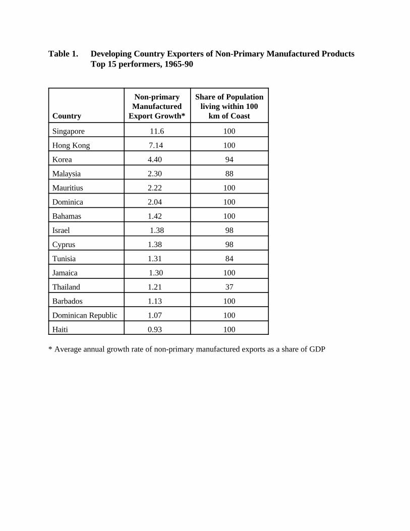
Table 1. Developing Country Exporters of Non-Primary Manufactured ProductsTop 15 performers, 1965-90

Country Export Growth* km of Coast

Non-primary Share of PopulationManufactured living within 100

Singapore 11.6 100

Hong Kong 7.14 100

Korea 4.40 94

Malaysia 2.30 88

Mauritius 2.22 100

Dominica 2.04 100

Bahamas 1.42 100

Israel 1.38 98

Cyprus 1.38 98

Tunisia 1.31 84

Jamaica 1.30 100

Thailand 1.21 37

Barbados 1.13 100

Dominican Republic 1.07 100

Haiti 0.93 100

* Average annual growth rate of non-primary manufactured exports as a share of GDP

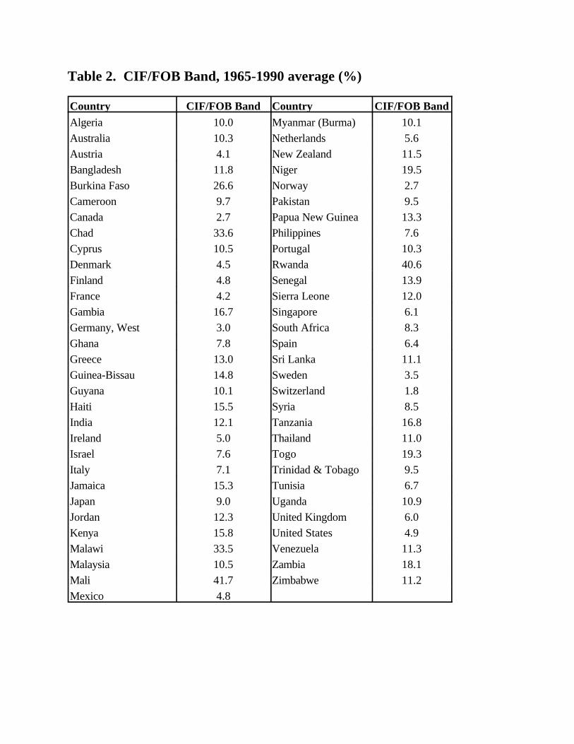
Table 2. CIF/FOB Band, 1965-1990 average (%)

Country CIF/FOB Band Country CIF/FOB BandAlgeria 10.0 Myanmar (Burma) 10.1

Australia 10.3 Netherlands 5.6

Austria 4.1 New Zealand 11.5

Bangladesh 11.8 Niger 19.5

Burkina Faso 26.6 Norway 2.7

Cameroon 9.7 Pakistan 9.5

Canada 2.7 Papua New Guinea 13.3

Chad 33.6 Philippines 7.6

Cyprus 10.5 Portugal 10.3

Denmark 4.5 Rwanda 40.6

Finland 4.8 Senegal 13.9

France 4.2 Sierra Leone 12.0

Gambia 16.7 Singapore 6.1

Germany, West 3.0 South Africa 8.3

Ghana 7.8 Spain 6.4

Greece 13.0 Sri Lanka 11.1

Guinea-Bissau 14.8 Sweden 3.5

Guyana 10.1 Switzerland 1.8

Haiti 15.5 Syria 8.5

India 12.1 Tanzania 16.8

Ireland 5.0 Thailand 11.0

Israel 7.6 Togo 19.3

Italy 7.1 Trinidad & Tobago 9.5

Jamaica 15.3 Tunisia 6.7

Japan 9.0 Uganda 10.9

Jordan 12.3 United Kingdom 6.0

Kenya 15.8 United States 4.9

Malawi 33.5 Venezuela 11.3

Malaysia 10.5 Zambia 18.1

Mali 41.7 Zimbabwe 11.2

Mexico 4.8

Table 3. Transport Costs, Coastal and Landlocked Countries in Africa

Based on export shipments in 1995, US dollars, per twenty-foot equivalent (TEU)

CoastalCountry Inland route Landlocked Country Northern Europe Japan North America

Destination

Senegal 1,610 4,100 n.a.

via Senegal: Mali 2,380 4,870 n.a.

additional cost (%) 48% 19%

Ghana 1,815 3,025 2,460

via Ghana: Burkina Faso 2,615 3,825 3,260

additional cost (%) 44% 26% 33%

Cameroon 1,520 n.a. n.a.

via Cameroon: Central African Rep. 2,560 n.a. n.a.

additional cost (%) 68%

Tanzania 1,380 1,350 2,000

via Tanzania by road: Rwanda 3,880 3,850 4,500

additional cost (%) 181% 185% 125%

Burundi 4,530 4,500 5,150

additional cost (%) 228% 233% 158%

Zambia 3,250 3,220 3,870

additional cost (%) 136% 139% 94%

Malawi 3,090 3,060 3,710

additional cost (%) 124% 127% 86%

via Tanzania by rail: Zambia 2,380 2,350 3,000

additional cost (%) 72% 74% 50%

Malawi 1,730 1,700 2,350

additional cost (%) 25% 26% 18%

Source: UNCTAD “Review of Maritime Transport 1995"

Table 4. Determinants of Shipping Costs

Dependent Variable: Shipping Cost (CIF/FOB band, log), 1965-1990 average

Independent CoefficientsVariable (t-statistics)

I II

Shipping Distance(log)

0.13 0.21(2.25) (3.17)

Landlocked 0.43 0.19(2.96) (0.60)

GDP per capita (1965, log)

-0.30(-4.38)

Port Quality -0.09(-1.36)

Number of Countries 61 31

Adjusted R 0.67 0.412

Note: Constant term not reported.

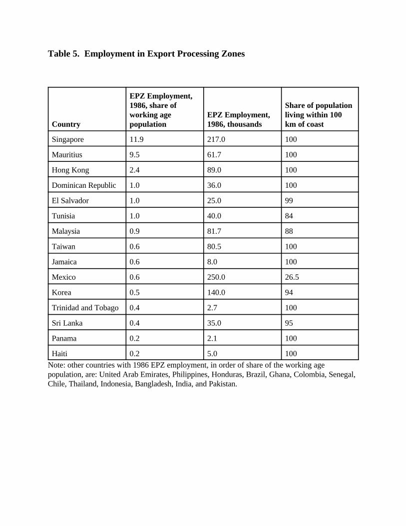
Table 5. Employment in Export Processing Zones

Country population 1986, thousands km of coast

EPZ Employment,1986, share of Share of populationworking age EPZ Employment, living within 100

Singapore 11.9 217.0 100

Mauritius 9.5 61.7 100

Hong Kong 2.4 89.0 100

Dominican Republic 1.0 36.0 100

El Salvador 1.0 25.0 99

Tunisia 1.0 40.0 84

Malaysia 0.9 81.7 88

Taiwan 0.6 80.5 100

Jamaica 0.6 8.0 100

Mexico 0.6 250.0 26.5

Korea 0.5 140.0 94

Trinidad and Tobago 0.4 2.7 100

Sri Lanka 0.4 35.0 95

Panama 0.2 2.1 100

Haiti 0.2 5.0 100

Note: other countries with 1986 EPZ employment, in order of share of the working agepopulation, are: United Arab Emirates, Philippines, Honduras, Brazil, Ghana, Colombia, Senegal,Chile, Thailand, Indonesia, Bangladesh, India, and Pakistan.

Table 6. Export Processing Zones: Imports, Exports, and Value Added

Imports/ Value Added/ Wages/Output (%) Output (%) Output (%)

Indonesia (1978-82) 61 n.a. n.a.

Malaysia (1975-82) 66 n.a. 8

Korea (1972-78) 54 30 n.a.

Philippines (1975-82) 61 31 14

Malaysian electronics (1982) 78 21 8

Malaysian textiles (1982) 49 13 9

Source: Warr (1984, 1987, 1989)

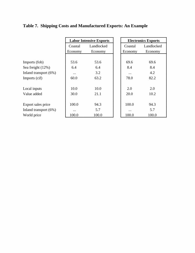
Table 7. Shipping Costs and Manufactured Exports: An Example

Labor Intensive Exports Electronics ExportsCoastal Landlocked Coastal Landlocked

Economy Economy Economy Economy

Imports (fob) 53.6 53.6 69.6 69.6 Sea freight (12%) 6.4 6.4 8.4 8.4 Inland transport (6%) ... 3.2 ... 4.2 Imports (cif) 60.0 63.2 78.0 82.2

Local inputs 10.0 10.0 2.0 2.0 Value added 30.0 21.1 20.0 10.2

Export sales price 100.0 94.3 100.0 94.3 Inland transport (6%) ... 5.7 ... 5.7 World price 100.0 100.0 100.0 100.0

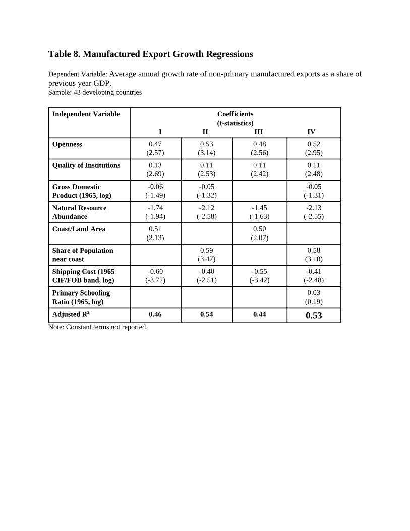
Table 8. Manufactured Export Growth Regressions

Dependent Variable: Average annual growth rate of non-primary manufactured exports as a share ofprevious year GDP. Sample: 43 developing countries

Independent Variable Coefficients(t-statistics)

I II III IV

Openness 0.47 0.53 0.48 0.52(2.57) (3.14) (2.56) (2.95)

Quality of Institutions 0.13 0.11 0.11 0.11(2.69) (2.53) (2.42) (2.48)

Gross DomesticProduct (1965, log)

-0.06 -0.05 -0.05(-1.49) (-1.32) (-1.31)

Natural ResourceAbundance

-1.74 -2.12 -1.45 -2.13(-1.94) (-2.58) (-1.63) (-2.55)

Coast/Land Area 0.51 0.50(2.13) (2.07)

Share of Populationnear coast

0.59 0.58(3.47) (3.10)

Shipping Cost (1965CIF/FOB band, log)

-0.60 -0.40 -0.55 -0.41(-3.72) (-2.51) (-3.42) (-2.48)

Primary SchoolingRatio (1965, log)

0.03(0.19)

Adjusted R 0.46 0.54 0.442 0.53Note: Constant terms not reported.

Table 9. Cross Country Growth RegressionsDependent Variable: Growth of real per capita GDP, 1965-90Sample: Developing Countries

Independent Variable Coefficients(t-statistics)

I II III IV

Initial GDPper capita (1965, log)

-1.73 -1.87 -1.84 -1.74(-7.00) (-7.86) (-6.21) (-4.94)

Life Expectancy (1965, log) 3.46 4.42 3.39 4.25(2.65) (3.99) (2.60) (2.76)

Primary Schooling Ratio(1965, log)

0.62 0.65 0.60 0.52(2.08) (2.14) (2.02) (1.09)

Openness 2.12 2.32 1.97 2.18(5.25) (5.87) (4.62) (4.70)

Government Savings Rate 0.14 0.14 0.14 0.17(4.97) (4.98) (4.94) (3.68)

Quality of Institutions 0.30 0.33 0.37 0.28(3.35) (3.80) (3.43) (2.46)

Growth of Working AgePopulation

0.80 0.45(1.81) (0.86)

Growth of Total Population -0.68 -0.36(-1.53) (-0.66)

Natural ResourceAbundance

-5.06 -5.01 -4.62 -8.24(-4.09) (-4.06) (-3.66) (-2.85)

Tropics -0.81 -0.80 -0.52 -0.41(-2.60) (-2.52) (-1.44) (-0.97)

Shipping Cost(CIF/FOB band, log)

-0.81 -0.89 -0.76 -1.28(-2.76) (-3.06) (-2.54) (-3.34)

Asia -0.44(-0.92)

Latin America -0.53(-1.12)

Sub-Saharan Africa -1.01(-1.82)

Number of Countries 64 64 64 41

Adjusted R 0.83 0.82 0.83 0.732

Note: Constant term not reported.