Stephen K. McNees

Vice President and Economist, FederalReserve Bank of Boston. Kiln Gilboand Delia Sawhney provided valuableresearch assistance. The author wouldlike to thank James S. Duesenberry forconstructive comments.

Just as consumers maximize their well-being (or "utility") subject totheir budget constraints and businesses maximize profits subject totechnological constraints, macroeconomic policymakers can, in prin-ciple, be viewed as maximizing policy goals, subject to feasibility

constraints imposed by the behavior of the household, business, andexternal sectors of the economy. For example, the central bank (hence-forth the Fed) can control some policy instrument quite precisely, eitherthe volume of (some measure of) bank reserves or a price (some short-terminterest rate). The policy instrument is manipulated to achieve the bestfeasible outcome in terms of the Fed’s ultimate objectives or policy goals.

In practice, the relationship between policy instruments and policygoals is highly uncertain and may be quite complex. Any linking ofpolicy instruments and policy goals, even a fixed nondiscretionary"rule," presumes,~at least implicitly, some knowledge of how themacroeconomy works. Clearly, experts disagree on how best to modelthe economy. In addition, monetary policy affects the economy onlyafter a lag. The policy decision made today has impacts months or evenyears in the future and therefore presumes, explicitly or implicitly, someforecast of future conditions. More fundamentally, economic policy mayhave several goals, each of which takes on a different importance atdifferent times, and these goals can come into conflict.

Given the uncertainties, numerous factors have been offered aspossible influences on monetary policy. Some have argued that policydepends importantly on the particular individual who is President ofthe United States or Chairman of the Fed, or on the political party inpower. Others have argued that monetary policy depends on the stanceof fiscal policy--as measured by the federal deficit, the debt, or gov-ernment spending. (See Dwyer 1985 for a review of this literature.) Itis widely believed that the Fed concentrates on stabilizing financialmarkets, such as the foreign exchange value of the dollar, securitiesprices, or interest rates.

This article develops a simpler approach; it findsthat monetary policy has been influenced by bothforecasts of and past experience with three broadfactors--inflation, economic activity, and the mone-tary aggregates. The degree of influence of eachfactor has, however, varied within this commontheme: in the past 22 years at least two specific shiftshave occurred, resulting in three "policy regimes."The most important shifts stemmed from differencesin the importance attached to the monetary aggre-gates, as well as from changes in the appropriatedefinition of "money." Other shifts may have oc-curred in policymakers’ forecast horizon and in theirpreferred measure of economic activity. This studyfinds no impact on policy from the particular individ-ual who is Chairman of the Fed or President of theUnited States, or from the political party holding thePresidency. It also finds no systematic reaction tovarious measures of fiscal policy, exchange rates, orstock prices.

Policy Goals, Instruments, and RegimesThe primary goals of monetary policy are fairly

evident low inflation and high levels of employ-ment and economic growth. Monetary policy hastended to "lean against the wind"--tightening wheninflation is high and easing when economic activity islow or falling. In addition, in its role as lender of lastresort, the Fed is concerned with stability in thefinancial markets. This abstract objective could takeseveral alternative concrete forms--stabilization ofexchange rates, stock prices, interest rates (in partic-ular, "even-keeling" during Treasury refundings), oreven the growth of some monetary aggregate. Thisstudy looks for evidence of each of these motives. Itfinds clear evidence of a role for money growth,mixed evidence for interest-rate smoothing, and littleevidence for the other potential objectives.

Attempts to describe the Fed’s behavior, to char-acterize it as "tight" or "easy," depend importantlyon which variable is assumed to be the instrument ofmonetary policy. If the Fed sets a short-term interestrate, the quantity of reserves (and money) will bedetermined endogenously by the public’s demand forreserves. In that case, attributing demand-drivenmovements in reserves (or money) to monetary pol-icy would result in spurious correlations. Similarly, ifthe Fed sets a reserve path, short-term interest ratesare determined by the demand for those reserves, sothat changes in interest rates cannot be attributed

directly to policy. The validity of empirical efforts tomodel monetary policy hinges critically on whetherthe policy instrument has been correctly identified.

The terminology of the theory of monetary policyhas become a morass. In an authoritative guide,Davis (1990, pp. 2-5) points out that policy instru-ments are on the opposite end of the spectrum fromthe "ultimate targets" of monetary policy. Examplesof instruments "include open market operations, thediscount rate, and in earlier periods, required reserveratios and Regulation Q ceilings on deposit interestrates. Just one step along the spectrum beyond theseinstruments are ’operating targets,’ measures thatcan be controlled with a rather high degree of preci-sion through manipulation of the policy instru-ments." Examples of "potential operating targetsinclude measures such as nonborrowed reserves, thenonborrowed monetary base, and short-term moneymarket rates, most notably the federal funds rate."

Even though open market operations are a purepolicy instrument, because the Fed has completecontrol over the quantity of securities it purchases orsells, the Fed’s "operating target," which cannot befixed exactly on a hourly, daily, or perhaps evenweekly basis, is a better empirical measure of themonetary policy instrument. First, some open marketoperations are purely "defensive" in nature; they areconducted simply to offset shocks to the reservemarket and have no implications for monetary policy.Second, the connotation of the word target in "oper-

The primary goals of monetarypolicy are fairly evident,-

low inflation and high levelsof employment andeconomic growth.

ating target" can be misleading. Target is commonlyused in association with both intermediate targets--such as monetary or credit aggregates or even nom-inal GNP--and the "ultimate targets" or policy goals.The essential dimension of the spectrum runningfrom policy instruments to policy goals (or "ultimatetargets") is the degree of precision with which themeasure can be controlled by policy. Clearly, control

4 November/December 1992 New England Economic Review

of intermediate targets and policy goals is highlyimprecise. In contrast, operating targets can be con-trolled with a very high degree of precision overperiods as long as a quarter, a month, or even a week.Because the focus of this inquiry is not the daily orweekly behavior of the Fed but rather its behavior ata quarterly frequency--the same frequency as GNPdata--referring to the "operating target" as a policyinstrument seems to be a useful simplification. Simi-larly, a finding that financial market variables do nothave an important influence on monetary policy at aquarterly frequency does not rule out the possibilitythat financial market variables could affect the daily,weekly, or even monthly timing within a calendarquarter.

Over the post-World War II period, there havebeen numerous changes in the Fed’s policy instru-ment. (See Meulendyke 1990 for a more completeaccount.) From World War II until the Treasury-Federal Reserve Accord in March 1951, the Fedpegged the yield of Treasury securities to minimizethe cost of Treasury financing. After the Accord,throughout most of the 1950s and 1960s, Fed atten-tion was focused on free reserves and short-termmoney market rates. (See Peele 1971, p. 154.) Theacceleration of inflation in the late 1960s led to strongcriticisms of the Fed’s interest-rate targeting proce-dures: rising nominal short-term rates should not beconstrued as a restrictive policy in an environment ofaccelerating inflation and money growth. (See, forexample, Friedman 1968.) In response to this dissat-isfaction, the Fed retained the federal funds rate asthe primary guide to day-to-day operations but, start-ing about 1970, formally adopted monetary growth asan intermediate target influencing the federal fundsrate. (See DeRosa and Stern 1977; Ribe 1979; Meu-lendyke 1990, pp. 461-62.) In contrast to an ultimatetarget or policy goal, an intermediate target is of nointrinsic importance but its behavior is thought to bean indicator, ideally an early indicator or predictor, ofthe ultimate policy goal. In this case, money growthwas used as a precursor of future inflation. Theenhanced attention to money growth was formalizedin a 1975 congressional resolution and embodied inThe Full Employment and Balanced Growth Act of1978, known as the Humphrey-Hawkins Act.

October 6, 1979 marks a clear and abrupt shift inmonetary policy’s operating procedures. Rising infla-tion, a falling dollar, and persistent overshooting ofthe M1 growth targets combined to cause a shift inemphasis to nonborrowed reserves, with an eyetoward greater control of money growth. This shift in

Figure 1

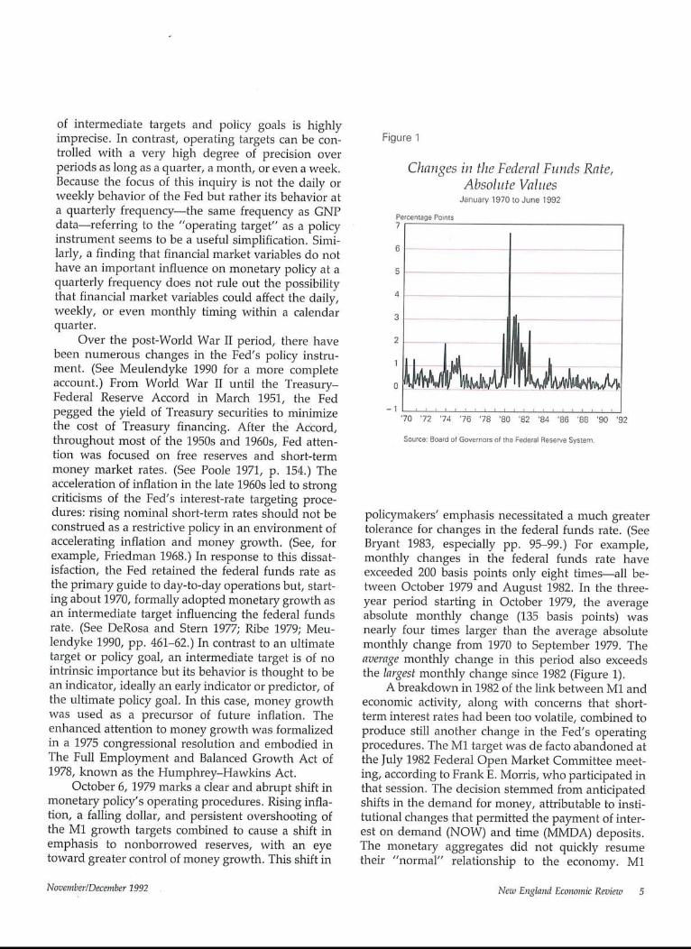
Changes in the Federal Funds Rate,Absolute Values

January 1970 to June 1992

Percentage Points7

6

5

4

3

2

1

0

-1’70 ’72 ’74 ’76 ’78 ’80 ’82 ’84 ’86 ’88 ’90 ’92

Source: Beard of Governors of the Federal Reserve S,/stern.

policymakers’ emphasis necessitated a much greatertolerance for changes in the federal funds rate. (SeeBryant 1983, especially pp. 95-99.) For example,monthly changes in the federal funds rate haveexceeded 200 basis points only eight times--all be-tween October 1979 and August 1982. In the three-year period starting in October 1979, the averageabsolute monthly change (135 basis points) wasnearly four times larger than the average absolutemonthly change from 1970 to September 1979. Theaverage monthly change in this period also exceedsthe largest monthly change since 1982 (Figure 1).

A breakdown in 1982 of the link between M1 andeconomic activity, along with concerns that short-term interest rates had been too volatile, combined toproduce still another change in the Fed’s operatingprocedures. The M1 target was de facto abandoned atthe July 1982 Federal Open Market Committee meet-ing, according to Frank E. Morris, who participated inthat session. The decision stemmed from anticipatedshifts in the demand for money, attributable to insti-tutional changes that permitted the payment of inter-est on demand (NOW) and time (MMDA) deposits.The monetary aggregates did not quickly resumetheir "normal" relationship to the economy. M1

November/December 1992 New England Economic Reviezo 5

growth vastly exceeded its long-run targets in both1985 and 1986, and in February 1987 M1 targets wereformally abandoned because of uncertainties aboutMl’s underlying relationship to the behavior of theeconomy and its sensitivity to economic and financialcircumstances.

With the demotion and eventual dismissal of M1targeting, M2 became the paramount monetary ag-gregate in Fed policy deliberations. At the same time,the relationship between M2 and economic activityhas not been sufficiently close to warrant relativelytight short-term targeting such as occurred fromOctober 1979 through 1982. In recent years, "In theabsence of a reliable intermediate target, the [Federal

Acknowledging that shifts have occurred, the econo-metric challenge is to see whether the differences canbe explicitly, formally modeled. One of the primaryuses of a model is as a base from which to measurechange. "Structural change" cannot be defined, letalone measured, without some conception of aninitial structure. Throughout most of the post-WorldWar II period, the primary instrument of monetarypolicy has been some short-term interest rate such asthe Treasury bill or federal funds rate. This articlecould be regarded as an investigation of whether aformal model can capture the variations in the policyinstrument and in the factors influencing policywithin a simple, underlying framework.

Acknowledging that shifts inpolicy regimes have occurred, the

econometric challenge is to seewhether the differences can beexplicitly, formally modeled.

Open Market] Committee has followed develop-ments of the economy and prices directly and hasobserved a variety of economic statistics, in additionto the monetary aggregates, that point to futuremoves in the goal variables" (Meulendyke 1990, p.471).

In short, two clear shifts in monetary policyoperating procedures have occurred since 1970, whenmonetary growth targets were first formally adopt-ed--the first in October 1979 and the second in mid1982, associated with the payment of interest on andchange in the definition of "money." In what follows,the period before October 1979 will be referred to as"regime one," the nearly three-year period afterOctober 1979 as "regime two," and the period sincemid 1982 as "regime three."

Different policy regimes can be studied empiri-cally in two different ways. In a strict sense, differentpolicy regimes, particularly those involving differentpolicy instruments, are independent, essentially non-comparable episodes. Each regime can only be stud-ied in isolation because each is technically a differentform of behavior. In contrast, it can be more infor-mative to try to incorporate these acknowledgeddifferences in behavior into a common framework.

The Data

All "actual" data--GNP, unemployment, and"money"--have been taken from contemporaneousdocuments, as opposed to the latest revisions, inorder to better represent the information available topolicymakers at the time their policy decisions weremade. The forecasts used are the ones prepared bythe staff of the Board of Governors and presented atFederal Open Market Committee meetings. Becausethese forecasts are not publicly available until fiveyears after the fact, the forecasts of a prominentcommercial forecasting service have been spliced onto complete the sample for recent years.

The ResultsTable 1 presents several versions of a federal

funds rate reaction function, fit to the period 1970:IIIto 1992:II. The first equation is the simplest, relatingthe federal funds rate (RFF) to its previous level andto actual values of the inflation rate (P), the unem-ployment rate (UR), real GNP growth (Q), and thequarterly growth rate of the narrow money stock(M1,1). Each of these variables has the expected signand is statistically significant at conventional levels ofsignificance. However, the "fit"--a 116-basis-pointstandard error--is only slightly better than that (128basis points) of a simple fourth-order autoregressionof the federal funds rate on its own lagged values.The fit can be improved about 22 percent--to a90-basis-point standard error--simply by allowingmoney growth to take on a different importance inthe three different regimes; note also that moneygrowth is measured by the one-quarter growth rate of

6 November/December 1992 New England Economic Review

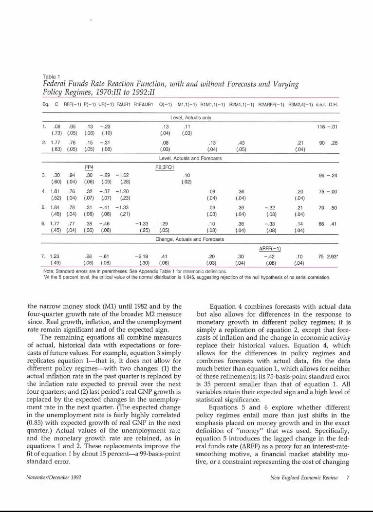
Table 1Federal Funds Rate Reaction Function, with and zoithout Forecasts and VaryingPolicy Regimes, 1970:Ili to 1992:1IEq. C RFF(-1) P(-1) UR(-1) FAUR1 R1F&UR1 Q(-1) M1,1(-1) RIM1,1(-1) R2M1,1(-1) R2&RFF(-1) R3M2,4(-1) s.e.r.D.H.

Level, Actuals only1. .08 .95 .13 -.23 .13 .11 116 -.01

(.73) (.05) (.06) (.10) (.04) (.03)

2. 1.77 .76 .15 -.31 .08 .13 .43 .21 90 .26(.63) (.05) (.05) (.08) (.03) (.04) (.05) (.04)

Level, Actuals and Forecasts

R2,3FQ1.10 99 -.24

(.02)

FP4

3. .30 .94 .30 -.29 -1.62(.60) (.04) (.06) (.09) (.28)

4. 1.81 .76 .32 -.37 -1.20(.52) (.04) (.07) (.07) (.23)

5. 1.84 .78 .31 -.41 -1.33(.48) (.04) (.06) (.06) (.21)

6. 1.77 .77 ,38 -.46(.45) (.04) (.06) (.06)

.09 .36 .20 75 -,00(.04) (.o4) (.04).09 .39 -.32 .21 70 .50

(.03) (.04) (.08) (.04)-1.33 .29 .10 .36 -.33 .14 66 .41

(.25) (.05) (.03) (,04) (.08) (.04)Change~ Actuals and Forecasts

f, RFF(- 1)7. 1.23 .28 -.61 -2.19 .41 .20 .30 -.42 .10 75 2.93*

(.49) (.06) (.08) (.30) (.06) (.03) (.04) (.08) (.04)Note: Standard errors are in parentheses. See Appendix Table 1 for mnemonic definitions."At the 5 percent level, the critical value of the normal distribution is 1.645, suggesting rejection of the null hypothesis of no serial correlation.

the narrow money stock (M1) until 1982 and by thefour-quarter growth rate of the broader M2 measuresince. Real growth, inflation, and the unemploymentrate remain significant and of the expected sign.

The remaining equations all combine measuresof actual, historical data with expectations or fore-casts of future values. For example, equation 3 simplyreplicates equation 1--that is, it does not allow fordifferent policy regimes--with two changes: (1) theactual inflation rate in the past quarter is replaced bythe inflation rate expected to prevail over the nextfour quarters; and (2) last period’s real GNP growth isreplaced by the expected changes in the unemploy-ment rate in the next quarter. (The expected changein the unemployment rate is fairly highly correlated(0.85) with expected growth of real GNP in the nextquarter.) Actual values of the unemployment rateand the monetary growth rate are retained, as inequations 1 and 2. These replacements improve thefit of equation 1 by about 15 percent--a 99-basis-pointstandard error.

Equation 4 combines forecasts with actual databut also allows for differences in the response tomonetary growth in different policy regimes; it issimply a replication of equation 2, except that fore-casts of inflation and the change in economic activityreplace their historical values. Equation 4, whichallows for the differences in policy regimes andcombines forecasts with actual data, fits the datamuch better than equation 1, which allows for neitherof these refinements; its 75-basis-point standard erroris 35 percent smaller than that of equation 1. Allvariables retain their expected sign and a high level ofstatistical significance.

Equations 5 and 6 explore whether differentpolicy regimes entail more than just shifts in theemphasis placed on money growth and in the exactdefinition of "money" that was used. Specifically,equation 5 introduces the lagged change in the fed-eral funds rate (~RFF) as a proxy for an interest-rate-smoothing motive, a financial market stability mo-tive, or a constraint representing the cost of changing

November/December 1992 Nezo England Economic Reviezo 7

the policy instrument. If one of these factors is atplay, the Fed will be more reluctant, other thingsequal, to continue to change interest rates in the samedirection as recent changes.

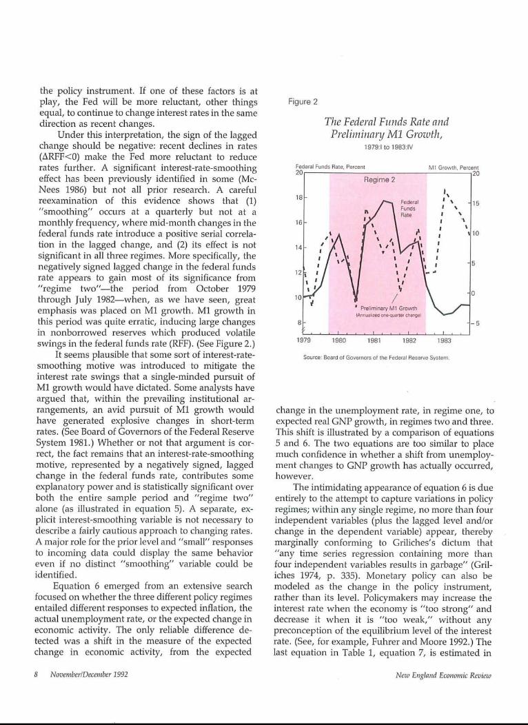
Under this interpretation, the sign of the laggedchange should be negative: recent declines in rates(ARFF<0) make the Fed more reluctant to reducerates further. A significant interest-rate-smoothingeffect has been previously identified in some (Mc-Nees 1986) but not all prior research. A carefulreexamination of this evidence shows that (1)"smoothing" occurs at a quarterly but not at amonthly frequency, where mid-month changes in thefederal funds rate introduce a positive serial correla-tion in the lagged change, and (2) its effect is notsignificant in all three regimes. More specifically, thenegatively signed lagged change in the federal fundsrate appears to gain most of its significance from"regime two"--the period from October 1979through July 1982--when, as we have seen, greatemphasis was placed on M1 growth. M1 growth inthis period was quite erratic, inducing large changesin nonborrowed reserves which produced volatileswings in the federal funds rate (RFF). (See Figure 2.)

It seems plausible that some sort of interest-rate-smoothing motive was introduced to mitigate theinterest rate swings that a single-minded pursuit ofM1 growth would have dictated. Some analysts haveargued that, within the prevailing institutional ar-rangements, an avid pursuit of M1 growth wouldhave generated explosive changes in short-termrates. (See Board of Governors of the Federal ReserveSystem 1981.) Whether or not that argument is cor-rect, the fact remains that an interest-rate-smoothingmotive, represented by a negatively signed, laggedchange in the federal funds rate, contributes someexplanatory power and is statistically significant overboth the entire sample period and "regime two"alone (as illustrated in equation 5). A separate, ex-plicit interest-smoothing variable is not necessary todescribe a fairly cautious approach to changing rates.A major role for the prior level and "small" responsesto incoming data could display the same behavioreven if no distinct "smoothing" variable could beidentified.

Equation 6 emerged from an extensive searchfocused on whether the three different policy regimesentailed different responses to expected inflation, theactual unemployment rate, or the expected change ineconomic activity. The only reliable difference de-tected was a shift in the measure of the expectedchange in economic activity, from the expected

Figure 2

The Federal Funds Rate andPreliminary M1 Growth,

1979:1 to 1983:1V

Federal Funds Rate, Percent

~8

16

14

Regime 2

[VII Growth, Percent2O

15

10

12

10

8

1979 1980 1981 1982 1983

Source: Board of Governors of the Federal Reserve System.

change in the unemployment rate, in regime one, toexpected real GNP growth, in regimes two and three.This shift is illustrated by a comparison of equations5 and 6. The two equations are too similar to placemuch confidence in whether a shift from unemploy-ment changes to GNP growth has actually occurred,however.

The intimidating appearance of equation 6 is dueentirely to the attempt to capture variations in policyregimes; within any single regime, no more than fourindependent variables (plus the lagged level and/orchange in the dependent variable) appear, therebymarginally conforming to Griliches’s dictum that"any time series regression containing more thanfour independent variables results in garbage" (Gril-iches 1974, p. 335). Monetary policy can also bemodeled as the change in the policy instrument,rather than its level. Policymakers may increase theinterest rate when the economy is "too strong" anddecrease it when it is "too weak," without anypreconception of the equilibrium level of the interestrate. (See, for example, Fuhrer and Moore 1992.) Thelast equation in Table 1, equation 7, is estimated in

8 November/Dece~nber 1992 New England Economic Review

change, rather than level, form. The change in thefederal funds rate is related to its own past value andto the same variables for inflation, economic activity,and money growth as are used in equation 6. Theoverall results are similar for the two formulations.The minor differences are that the interest-rate-smoothing variable--the negatively signed change--is significant in all regimes, while the role of M1growth is larger in regime one, and the expectedchange in the employment rate is more important.

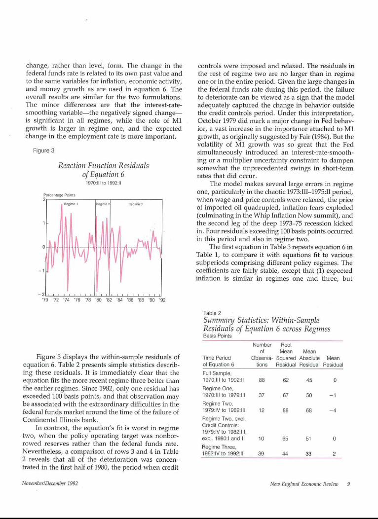
Figure 3

Reaction Function Residualsof Equation 6

1970:111 to 1992:11

Percentage Points2

Regime

1

Regime

’70 ’72 ’74 ’76 ’78 ’80 ’82

Regime 3

’84 ’86 ’88 ’90 ’92

controls were imposed and relaxed. The residuals inthe rest of regime two are no larger than in regimeone or in the entire period. Given the large changes inthe federal funds rate during this period, the failureto deteriorate can be viewed as a sign that the modeladequately captured the change in behavior outsidethe credit controls period. Under this interpretation,October 1979 did mark a major change in Fed behav-ior, a vast increase in the importance attached to M1growth, as originally suggested by Fair (1984). But thevolatility of M1 growth was so great that the Fedsimultaneously introduced an interest-rate-smooth-ing or a multiplier uncertainty constraint to dampensomewhat the unprecedented swings in short-termrates that did occur.

The model makes several large errors in regimeone, particularly in the chaotic 1973:III-1975:II period,when wage and price controls were relaxed, the priceof imported oil quadrupled, inflation fears exploded(culminating in the Whip Inflation Now summit), andthe second leg of the deep 1973-75 recession kickedin. Four residuals exceeding 100 basis points occurredin this period and also in regime two.

The first equation in Table 3 repeats equation 6 inTable 1, to compare it with equations fit to varioussubperiods comprising different policy regimes. Thecoefficients are fairly stable, except that (1) expectedinflation is similar in regimes one and three, but

Figure 3 displays the within-sample residuals ofequation 6. Table 2 presents simple statistics describ-ing these residuals. It is immediately clear that theequation fits the more recent regime three better thanthe earlier regimes. Since 1982, only one residual hasexceeded 100 basis points, and that observation maybe associated with the extraordinary difficulties in thefederal funds market around the time of the failure ofContinental Illinois bank.

In contrast, the equation’s fit is worst in regimetwo, when the policy operating target was nonbor-rowed reserves rather than the federal funds rate.Nevertheless, a comparison of rows 3 and 4 in Table2 reveals that all of the deterioration was concen-trated in the first half of 1980, the period when credit

Table 2Summary Statistics: Within-SampleResiduals of Equation 6 across RegimesBasis Points

Number Rootof Mean Mean

Time Period Observa- Squared Absolute Meanof Equation 6 tions Residual Residual ResidualFull Sample,1970:111 to 1992:11 88 62 45 0Regime One,1970:111 to 1979:111 37 67 50 -1Regime Two,1979:1V to 1982:111 12 88 68 -4Regime Two, excl.Credit Controls:1979:1V to 1982:111,excl. 1980:1 and II 10 65 51 0Regime Three,1982:1V to 1992:11 39 44 33 2

November/December 1992 New England Economic Review 9

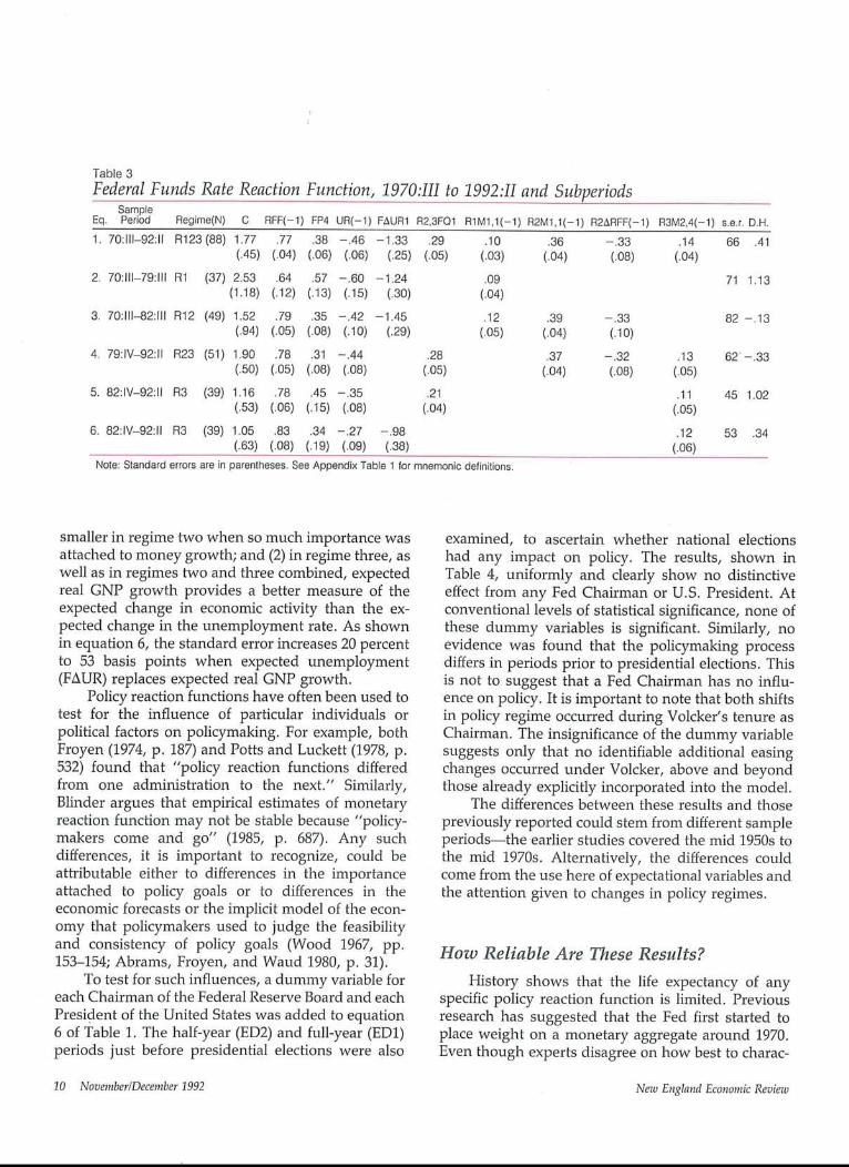
Table 3Federal Funds RateReaction

SampleEq. Period Regime(N) C RFF(-1)

1. 70:111-92:11 R123 (88) 1.77 .77 .38 -.46 -1.33(.45) (.04) (.06) (.06) (.25)

2. 70:111-79:111 R1 (37) 2.53 .64 .57 -.60 -1.24(1.18) (.12) (.13) (.15) (.30)

3. 70:111~2:111 R12 (49) 1.52 .79 .35 -.42 -1.45(.94) (.05) (.08) (.10) (.29)

4. 79:1V-92:11 R23 (51) 1.90 .78 .31 -.44(.50) (.05) (.08) (.08)

5. 82:1V-92:11 R3 (39) 1.16 .78 .45 -.35(.53) (.06) (.15) (.08)

Function, 1970:111 to 1992:II and Subperiods

FP4 UR(-1) F&UR1 R2,3FQ1 RIM1,1(-1) R2Ml,1(-1) R2&RFF(-1) R3M2,4(-1) s.e.r.D.H.

.29 .36 -.33 .14 66 .41(.05) (.04) (.08) (.04)

71 1.13

.28(.05)

.21(.04)

.10(.03)

.09(.04).12

(.o5).39 -.33

(.04) (.10)

.37 -.32(.04) (.08)

6. 82:1V-92:11 R3 (39) 1.05 .83 .34 -.27 -.98(.63) (.08) (.19) (.09) (.38)

Note: Standard errors are in parentheses. See Appendix Table 1 for mnemonic definitions.

82 -.13

.13 62 -,33(.o5)

.11 45 1.02(.05)

.12 53 .34(.o6)

smaller in regime two when so much importance wasattached to money growth; and (2) in regime three, aswell as in regimes two and three combined, expectedreal GNP growth provides a better measure of theexpected change in economic activity than the ex-pected change in the unemployment rate. As shownin equation 6, the standard error increases 20 percentto 53 basis points when expected unemployment(F/~UR) replaces expected real GNP growth.

Policy reaction functions have often been used totest for the influence of particular individuals orpolitical factors on policymaking. For example, bothFroyen (1974, p. 187) and Potts and Luckett (1978, p.532) found that "policy reaction functions differedfrom one administration to the next." Similarly,Blinder argues that empirical estimates of monetaryreaction function may not be stable because "policy-makers come and go" (1985, p. 687). Any suchdifferences, it is important to recognize, could beattributable either to differences in the importanceattached to policy goals or to differences in theeconomic forecasts or the implicit model of the econ-omy that policymakers used to judge the feasibilityand consistency of policy goals (Wood 1967, pp.153-154; Abrams, Froyen, and Waud 1980, p. 31).

To test for such influences, a dummy variable foreach Chairman of the Federal Reserve Board and eachPresident of the United States was added to equation6 of Table 1. The half-year (ED2) and full-year (ED1)periods just before presidential elections were also

examined, to ascertain whether national electionshad any impact on policy. The results, shown inTable 4, uniformly and clearly show no distinctiveeffect from any Fed Chairman or U.S. President. Atconventional levels of statistical significance, none ofthese dummy variables is significant. Similarly, noevidence was found that the policymaking processdiffers in periods prior to presidential elections. Thisis not to suggest that a Fed Chairman has no influ-ence on policy. It is important to note that both shiftsin policy regime occurred during Volcker’s tenure asChairman. The insignificance of the dummy variablesuggests only that no identifiable additional easingchanges occurred under Volcker, above and beyondthose already explicitly incorporated into the model.

The differences between these results and thosepreviously reported could stem from different sampleperiods--the earlier studies covered the mid 1950s tothe mid 1970s. Alternatively, the differences couldcome from the use here of expectational variables andthe attention given to changes in policy regimes.

How Reliable Are These Results?

History shows that the life expectancy of anyspecific policy reaction function is limited. Previousresearch has suggested that the Fed first started toplace weight on a monetary aggregate around 1970.Even though experts disagree on how best to charac-

10 November/December 1992 New England Economic Review

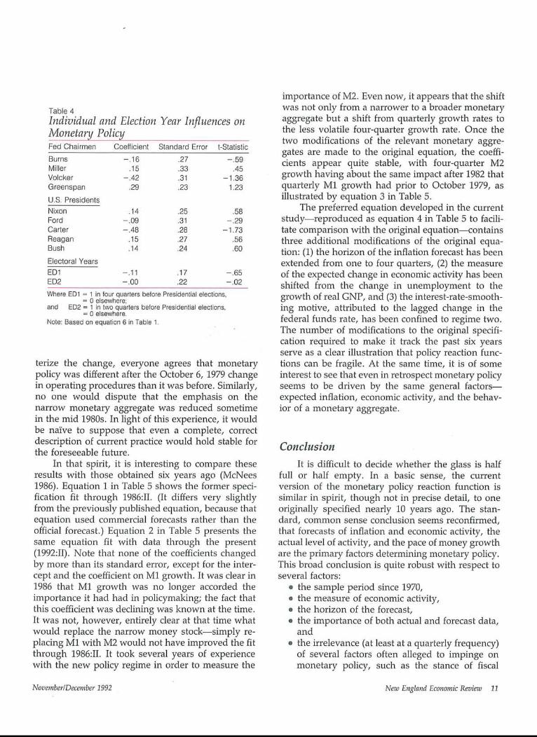
Table 4Individual and Election Year Influences onMonetar~j Polic~ ........Fed Chairmen

BurnsMillerVolckerGreenspan

U.S. PresidentsNixonFordCarterReaganBush

Coefficient Standard Error t-Statistic-.16 .27 -.59

.15 .33 .45-.42 .31 -1.36

.29 .23 1.23

.14 .25 .58-.09 .31 -.29-.48 .28 -1.73

.15 .27 .56

.14 .24 .60Electoral YearsED1 -.11 .17 -.65ED2 -.00 .22 -.02Where ED1 = 1 in four quarters before Presidential elections,

= 0 elsewhere;and ED2 = 1 in two quarters before Presidential elections,

= 0 elsewhere.Note: Based on equation 6 in Table 1.

terize the change, everyone agrees that monetarypolicy was different after the October 6, 1979 changein operating procedures than it was before. Similarly,no one would dispute that the emphasis on thenarrow monetary aggregate was reduced sometimein the mid 1980s. In light of this experience, it wouldbe naive to suppose that even a complete, correctdescription of current practice would hold stable forthe foreseeable future.

In that spirit, it is interesting to compare theseresults with those obtained six years ago (McNees1986). Equation 1 in Table 5 shows the former speci-fication fit through 1986:II. (It differs very slightlyfrom the previously published equation, because thatequation used commercial forecasts rather than theofficial forecast.) Equation 2 in Table 5 presents thesame equation fit with data through the present(1992:I0. Note that none of the coefficients changedby more than its standard error, except for the inter-cept and the coefficient on M1 growth. It was clear in1986 that M1 growth was no longer accorded theimportance it had had in policymaking; the fact thatthis coefficient was declining was known at the time.It was not, however, entirely clear at that time whatwould replace the narrow money stock---simply re-placing M1 with M2 would not have improved the fitthrough 1986:II. It took several years of experiencewith the new policy regime in order to measure the

importance of M2. Even now, it appears that the shiftwas not only from a narrower to a broader monetaryaggregate but a shift from quarterly growth rates tothe less volatile four-quarter growth rate. Once thetwo modifications of the relevant monetary aggre-gates are made to the original equation, the coeffi-cients appear quite stable, with four-quarter M2growth having about the same impact after 1982 thatquarterly M1 growth had prior to October 1979, asillustrated by equation 3 in Table 5.

The preferred equation developed in the currentstudy--reproduced as equation 4 in Table 5 to facili-tate comparison with the original equation---containsthree additional modifications of the original equa-tion: (1) the horizon of the inflation forecast has beenextended from one to four quarters, (2) the measureof the expected change in economic activity has beenshifted from the change in unemployment to thegrowth of real GNP, and (3) the interest-rate-smooth-ing motive, attributed to the lagged change in thefederal funds rate, has been confined to regime two.The number of modifications to the original specifi-cation required to make it track the past six yearsserve as a clear illustration that policy reaction func-tions can be fragile. At the same time, it is of someinterest to see that even in retrospect monetary policyseems to be driven by the same general factors--expected inflation, economic activity, and the behav-ior of a monetary aggregate.

ConclusionIt is difficult to decide whether the glass is half

full or half empty. In a basic sense, the currentversion of the monetary policy reaction function issimilar in spirit, though not in precise detail, to oneoriginally specified nearly 10 years ago. The stan-dard, common sense conclusion seems reconfirmed,that forecasts of inflation and economic activity, theactual level of activity, and the pace of money growthare the primary factors determining monetary policy.This broad conclusion is quite robust with respect toseveral factors:

¯ the sample period since 1970,¯ the measure of economic activity,¯ the horizon of the forecast,¯ the importance of both actual and forecast data,

and¯ the irrelevance (at least at a quarterly frequency)

of several factors often alleged to impinge onmonetary policy, such as the stance of fiscal

November/December 1992 New England Economic Review 11

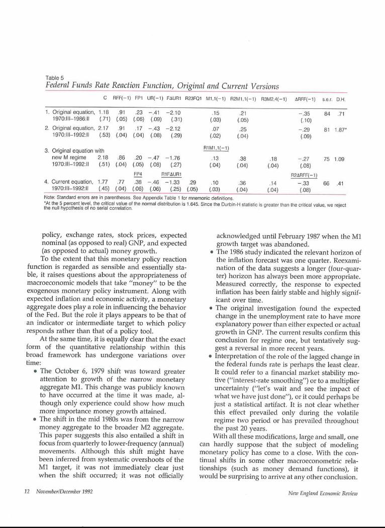
Table 5

_Fe~der_al Funds Rate Reaction Function, Original and Current VersionsC RFF(-1) FP1 UR(-1) F~UR1 R23FQ1 M1,1(-1) R2M1,1(-1) R3M2,4(-1) &RFF(-1) s.e.r.D.H.

1. Original equation, 1.18 .91 .23 -.41 -2.10 .15 .21 -.35 84 .711970:111-1986:11 (.71) (.05) (.06) (.09) (.31) (.03) (.05) (.10)

2. Original equation, 2.17 .91 .17 -.43 -2.12 .07 .25 -.29 81 1.87"1970:111-1992:11 (.53) (.04) (.04) (.08) (.29) (.02) (.04) (.09)

3. Original equation with RIM1,1(-1!

newMregime 2.18 .86 .20 -.47 -1.76 .13 .38 .18 -.27 75 1.091970:111-1992:11 (.51) (.04) (.05) (.08) (.27) (.04) (.04) (.04) (.08)

FP._~_4 R1F&UR1 R2&RFF(-I!4. Current equation, 1.77 .77 .38 -.46 -1.33 .29 .10 .36 .14 -.33 66 .41

1970:111-1992:11 (.45) (.04) (.06) (.06) (.25) (.05) (.03) (.04) (.04) (.08)Note: Standard errors are in parentheses. See Appendix Table 1 for mnemonic definitions."At the 5 percent level, the critical value of the normal distribulion is 1.645. Since the Durbin-H statistic is greater than the critical value, we rejectthe null hypothesis of no serial correlation.

policy, exchange rates, stock prices, expectednominal (as opposed to real) GNP, and expected(as opposed to actual) money growth.To the extent that this monetary policy reaction

function is regarded as sensible and essentially sta-ble, it raises questions about the appropriateness ofmacroeconomic models that take "money" to be theexogenous monetary policy instrument. Along withexpected inflation and economic activity, a monetaryaggregate does play a role in influencing the behaviorof the Fed. But the role it plays appears to be that ofan indicator or intermediate target to which policyresponds rather than that of a policy tool.

At the same time, it is equally clear that the exactform of the quantitative relationship within thisbroad framework has undergone variations overtime:

¯ The October 6, 1979 shift was toward greaterattention to growth of the narrow monetaryaggregate M1. This change was publicly knownto have occurred at the time it was made, al-though only experience could show how muchmore importance money growth attained.

¯ The shift in the mid 1980s was from the narrowmoney aggregate to the broader M2 aggregate.This paper suggests this also entailed a shift infocus from quarterly to lower-frequency (annual)movements. Although this shift might havebeen inferred from systematic overshoots of theM1 target, it was not immediately clear justwhen the shift occurred; it was not officially

acknowledged until February 1987 when the M1growth target was abandoned.

¯ The 1986 study indicated the relevant horizon ofthe inflation forecast was one quarter. Reexami-nation of the data suggests a longer (four-quar-ter) horizon has always been more appropriate.Measured correctly, the response to expectedinflation has been fairly stable and highly signif-icant over time.

¯ The original investigation found the expectedchange in the unemployment rate to have moreexplanatory power than either expected or actualgrowth in GNP. The current results confirm thisconclusion for regime one, but tentatively sug-gest a reversal in more recent years.

¯ Interpretation of the role of the lagged change inthe federal funds rate is perhaps the least clear.It could refer to a financial market stability mo-tive ("interest-rate smoothing") or to a multiplieruncertainty ("let’s wait and see the impact ofwhat we have just done"), or it could perhaps bejust a statistical artifact. It is not clear whetherthis effect prevailed only during the volatileregime two period or has prevailed throughoutthe past 20 years.With all these modifications, large and small, one

can hardly suppose that the subject of modelingmonetary policy has come to a close. With the con-tinual shifts in some other macroeconometric rela-tionships (such as money demand functions), itwould be surprising to arrive at any other conclusion.

12 November/December 1992 New England Economic Reviezo

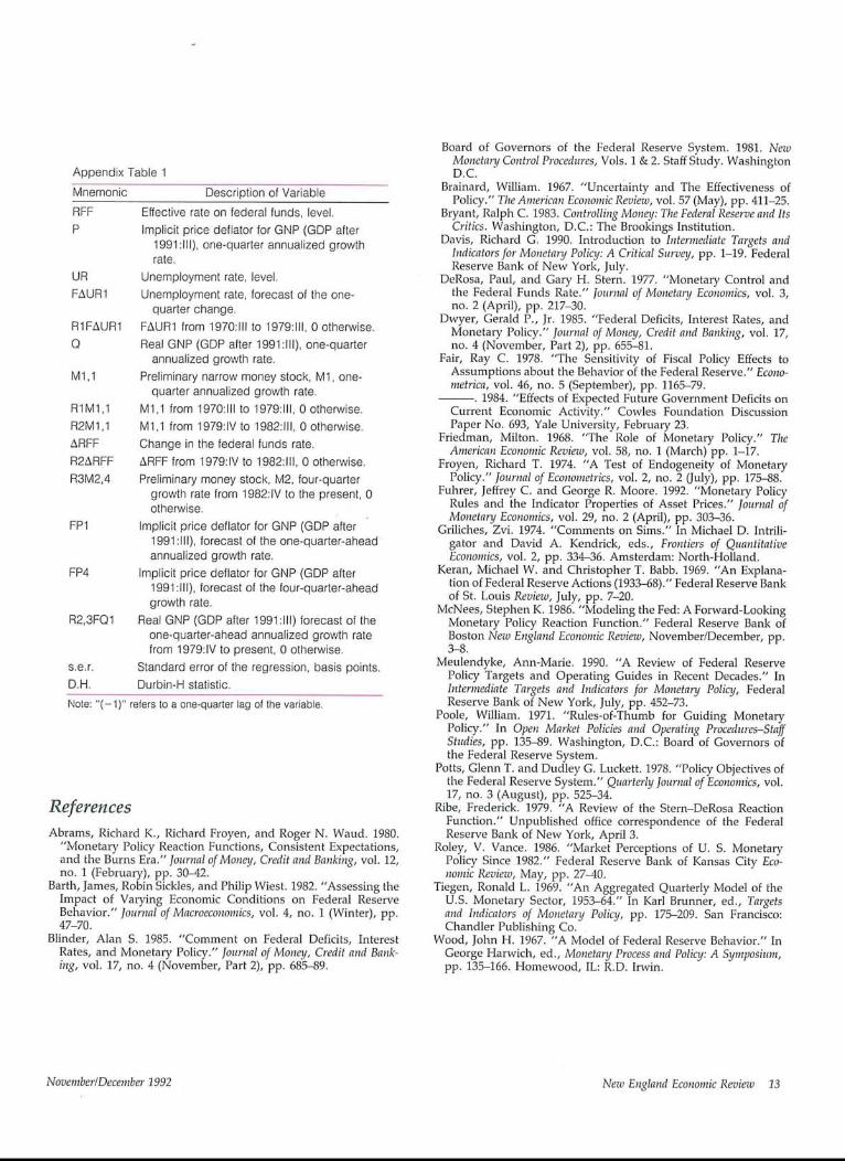
Appendix Table 1

Mnemonic Description of VariableRFF Effective rate on federal funds, level.P Implicit price deflator for GNP (GDP after

1991:111), one-quarter annualized growthrate.

UR Unemployment rate, level.F,~UR1 Unemployment rate, forecast of the one-

quarter change.R1FAUR1 FAURI from 1970:111 to 1979:111, 0 otherwise.Q Real GNP (GDP after 1991:111), one-quarter

annualized growth rate.M1,1 Preliminary narrow money stock, M1, one-

quarter annualized growth rate.R1M1,1 M1,1 from 1970:111 to 1979:111, 0 otherwise.R2Ml,1 M1,1 from 1979:1V to 1982:111, 0 otherwise.,&RFF Change in the federal funds rate.R2ARFF &RFF from 1979:1V to 1982:111, 0 otherwise.R3M2,4 Preliminary money stock, M2, four-quarter

growth rate from 1982:1V to the present, 0otherwise.

FP1 Implicit price deflator for GNP (GDP after1991:111), forecast of the one-quarter-aheadannualized growth rate.

FP4 Implicit price deflator for GNP (GDP after1991:111), forecast of the four-quarter-aheadgrowth rate.

R2,3FQ1 Real GNP (GDP after 1991:111) forecast of theone-quarter-ahead annualized growth ratefrom 1979:1V to present, 0 otherwise.

s.e.r. Standard error of the regression, basis points.D.H. Durbin-H statistic.Note: "(-1)" refers to a one-quarter lag of the variable.

ReferencesAbrams, Richard K., Richard Froyen, and Roger N. Waud. 1980.

"Monetary Policy Reaction Functions, Consistent Expectations,and the Burns Era." Journal of Money, Credit and Banking, vot. 12,no. 1 (February), pp. 3(~42.

Barth, James, Robin Sickles, and Philip Wiest. 1982. "Assessing theImpact of Varying Economic Conditions on Federal ReserveBehavior." Journal of Macroeconomics, vol. 4, no. 1 (Winter), pp.47-70.

Blinder, Alan S. 1985. "Comment on Federal Deficits, InterestRates, and Monetary Policy." Journal of Money, Credit and Bank-ing, vol. 17, no. 4 (November, Part 2), pp. 685~9.

Board of Governors of the Federal Reserve System. 1981. NewMoneta~d Control Procedures, Vols. 1 & 2. Staff Study. WashingtonD.C.

Brainard, William. 1967. "Uncertainty and The Effectiveness ofPolicy." The American Economic Review, vol. 57 (May), pp. 411-25.

Bryant, Ralph C. 1983. Controlling Money: The Federal Reserve and ItsCritics. Washington, D.C.: The Brookings Institution.

Davis, Richard G. 1990. Introduction to Intermediate Targets andIndicators for Monetary Policy: A Critical Survey, pp. 1-19. FederalReserve Bank of New York, July.

DeRosa, Paul, and Gary H. Stern. 1977. ’qVlonetary Control andthe Federal Funds Rate." Journal of Monetatlj Economics, vol. 3,no. 2 (April), pp. 217-30.

Dwyer, Gerald P., Jr. 1985. "Federal Deficits, Interest Rates, andMonetary Policy." Journal of Money, Credit and Banking, vol. 17,no. 4 (November, Part 2), pp. 655-81.

Fair, Ray C. 1978. "The Sensitivity of Fiscal Policy Effects toAssumptions about the Behavior of the Federal Reserve." Econo-metrica, vol. 46, no. 5 (September), pp. 1165-79.

--. 1984. "Effects of Expected Future Government Deficits onCurrent Economic Activity." Cowles Foundation DiscussionPaper No. 693, Yale University, February 23.

Friedman, Milton. 1968. "The Role of Monetary Policy." TheAmerican Economic Review, vol. 58, no. 1 (March) pp. 1-17.

Froyen, Richard T. 1974. "A Test of Endogeneity of MonetaryPolicy." Journal of Econometrics, vol. 2, no. 2 (July), pp. 17,%88.

Fuhrer, Jeffrey C. and George R. Moore. 1992. "Monetary PolicyRules and the Indicator Properties of Asset Prices." Journal ofMonetand Economics, vol. 29, no. 2 (April), pp. 303-36.

Griliches, Zvi. 1974. "Comments on Sims." In Michael D. Intrili-gator and David A. Kendrick, eds., Frontiers of QuantitativeEconomics, vol. 2, pp. 334-36. Amsterdam: North-Holland.

Keran, Michael W. and Christopher T. Babb. 1969. "An Explana-tion of Federal Reserve Actions (1933-68)." Federal Reserve Bankof St. Louis Review, July, pp. 7-20.

McNees, Stephen K. 1986. "Modeling the Fed: A Forward-LookingMonetary Policy Reaction Function." Federal Reserve Bank ofBoston New England Economic Review, November/December, pp.3-8.

Meulendyke, Ann-Marie. 1990. "A Review of Federal ReservePolicy Targets and Operating Guides in Recent Decades." InIntermediate Targets and Indicators for Monetanj Policy, FederalReserve Bank of New York, July, pp. 452-73.

Poole, William. 1971. "Rules-of-Thumb for Guiding MonetaryPolicy." In Open Market Policies and Operating Procedures-StaffStudies, pp. 135-89. Washington, D.C.: Board of Governors ofthe Federal Reserve System.

Potts, Glenn T. and Dudley G. Luckett. 1978. "Policy Objectives ofthe Federal Reserve System." Quarterly Journal of Economics, vol.17, no. 3 (August), pp. 525-34.

Ribe, Frederick. 1979. "A Review of the Stern-DeRosa ReactionFunction." Unpublished office correspondence of the FederalReserve Bank of New York, April 3.

Roley, V. Vance. 1986. "Market Perceptions of U. S. MonetaryPolicy Since 1982." Federal Reserve Bank of Kansas City Eco-nomic Review, May, pp. 27-40.

Tiegen, Ronald L. 1969. "An Aggregated Quarterly Model of theU.S. Monetary Sector, 195~64." In Karl Brunner, ed., Targetsand Indicators of Monetary Policy, pp. 175-209. San Francisco:Chandler Publishing Co.

Wood, John H. 1967. "A Model of Federal Reserve Behavior." InGeorge Harwich, ed., Monetary Process and Policy: A Symposium,pp. 135-166. Homewood, IL: R.D. Irwin.

November/December 1992 New England Economic Review 13