Steganographic Application of improved Genetic Shifting algorithm against RS analysis - BScEE final...
105
המחלקה להנדסת חשמל ואלקטרוניקה שם הפרויקטGenetic Shifting algorithm Steganographic Application of improved against RS analysis RS יישום של אלגוריתם סטגנוגרפי משופר להזזה גנטית להתמודדות מול ניתוח פרויקט הנדסי דו" ח מסכם הוכן לשם השלמת הדרישות לקבלת תואר ראשון בהנדסהB. Sc מאת פורינסון ודים307716068 בהנחייתMScEE קפלן ולדיסלב הוגש למחלקה להנדסת חשמל ואלקטרוניקה המכללה האקדמית להנדסה סמי שמעון באר- שבע תמוז תש ע" ה יולי2015
-
Upload
vladislav-kaplan -
Category
Engineering
-
view
13 -
download
1
Transcript of Steganographic Application of improved Genetic Shifting algorithm against RS analysis - BScEE final...

המחלקה להנדסת חשמל ואלקטרוניקה
שם הפרויקט
Genetic Shifting algorithm Steganographic Application of improved
against RS analysis
RS יישום של אלגוריתם סטגנוגרפי משופר להזזה גנטית להתמודדות מול ניתוח
פרויקט הנדסי
מסכםח "דו
B. Sc הוכן לשם השלמת הדרישות לקבלת תואר ראשון בהנדסה
מאת
307716068פורינסון ודים
בהנחיית
MScEE קפלן ולדיסלב
ואלקטרוניקה הוגש למחלקה להנדסת חשמל
סמי שמעון המכללה האקדמית להנדסה
שבע-באר
2015יולי ה"עתמוז תש

המחלקה להנדסת חשמל ואלקטרוניקה
שם הפרויקט
Application of improved Steganographic Genetic Shifting algorithm
against RS analysis
RS יישום של אלגוריתם סטגנוגרפי משופר להזזה גנטית להתמודדות מול ניתוח
פרויקט הנדסי
ח מסכם"דו
הוכן לשם השלמת הדרישות לקבל
תואר ראשון בהנדסה
מאת
פורינסון ודים 307716068
בהנחיית המנחה
MScEE קפלן ולדיסלב
הוגש למחלקה להנדסת חשמל ואלקטרוניקה
המכללה האקדמית להנדסה סמי שמעון
שבע-באר
תאריך לועזי תאריך עברי

המחלקה להנדסת חשמל ואלקטרוניקה
הפרויקט שם
Application of improved Steganographic Genetic Shifting algorithm
against RS analysis
RS יישום של אלגוריתם סטגנוגרפי משופר להזזה גנטית להתמודדות מול ניתוח
פרויקט הנדסי
ח מסכם"דו
הוכן לשם מילוי דרישות חלקיות לקבלת
תואר ראשון בהנדסה
מאת
פורינסון ודים 307716068
בהנחיית המנחה
MScEEקפלן ולדיסלב
הוגש למחלקה להנדסת חשמל ואלקטרוניקה
המכללה האקדמית להנדסה סמי שמעון
שבע-באר
: ______________חתימת הסטודנט : ________תאריך
: ______________חתימת המנחה : ________תאריך
: _________הפרויקטיםאישור ועדת : ________תאריך

המחלקה להנדסת חשמל ואלקטרוניקה
:תחום הפרויקט
(Image and Video Processing) תמונות ווידאו עיבוד
(Communications) תקשורת
:סוג הפרויקט
(Implementation) תכנון
(Research) מחקר
Key words:
Steganography, Steganalysis, Digital image, LSB, RS analysis, Genetic
algorithm.

המחלקה להנדסת חשמל ואלקטרוניקה
תקציר
, בניגוד לקריפטוגרפיה אשר מתעסקת בקידוד מידע. שיטה להסתרת מידע נמסר", מדע"סטגנוגרפיה היא
סטגנוגרפיה מטביעה את המסר . הרעיון העקרי של סטגנוגרפיה הוא הסתרת העובדה כי המסר קיים
עם התפתחות , במהלך השנים האחרונות'(. טקסט וכו, וידאו, קובץ שמע, תמונה)הסמוי במדיה דיגיטלית
שיטת הסטגנוגרפיה . שיטות סטגנוגרפיה דיגיטלית צברו פופולריות רבה, יכולות עיבוד תמונות דיגיטליות
עם האבולוציה . בתמונת המעטפת nt Bit)LSB (Last Significa -השכיחה ביותר היא החלפת ה
תפקיד האלגוריתם של הסטגואנליזה . לשיטות הסטגואנליזה חשיבות רבה, הנרחבת של הסטגנוגרפיה
RS-אלגורתים הסטגואנליזה המכובד ביותר הוא שיטת ה. הוא לגלות מסר סמוי בתוך כל סוג של מדיה
שן וואנג . סטטיסטי המיושם על גבי הפיקסלים של תמונהאשר מגלה מסר סטגנוגרפי על ידי ניתוח [, 1]
מבצעת Genetic Shifting method (GSM) .GSMיצרו אלגורתים חדש המבוסס על [ 2]ואחרים
שומר על הסטטיסטיקה של GSM-אלגוריתם ה. מניפולציה ושינוי של הפיקסלים בתמונה המקורית
מטרת הפרוייקט היא להראות . RS-ידי שיטת ה וקשה לגילוי על, התמונה לאחר הטבעת המסר הסמוי
על ידי שימוש בשיטות מתמטיות RS-כנגד שיטת ה GSM-את היעילות והיציבות של אלגוריתם ה
.וסטטיסטיות

המחלקה להנדסת חשמל ואלקטרוניקה
Abstract
Steganography is a “science”, the method of hiding sent information. Unlike cryptography that
deals with coding of information, the main idea of steganography is hiding the fact that the message
exists. It embeds the secret message in cover media (image, audio, video, text, etc.). During the
last years with the development of digital image processing, methods of digital steganography
have gained a lot of popularity. The most popular steganography method is LSB (Last Significant
Bit) replacement in the cover image. With extensive evolution of steganography, Steganalysis
methods have a lot of importance. Steganalysis algorithms role is to detect a hidden secret message
inside any media. The most notable Steganalysis algorithm is the RS method [1], which detects
stegamesage by the statistical analysis applied on image pixels.
Shen Wang and others [2] created a new algorithm based on Genetic Shifting method (GSM).
GSM performs manipulation and modification of the original image pixels. GSM algorithm keeps
image statistic after inserting a hidden message and is hard to be detected by the RS analysis. The
goal of the project is to demonstrate effectiveness and stability of GSM algorithm against RS
analysis by using mathematical and statistical methods.

המחלקה להנדסת חשמל ואלקטרוניקה
Table of Contents
1. Introduction……………………..……………………………………….….……………........1
1.1 Background…………………………………..…………………………….…….…….….......1
1.2 Applications and usage..…………………………………………………...….……….….......1
1.3 Digital steganography advantage…………………..…………………………….……...…….2
1.4 Engineering problem…..……………………………..………………….….…….……….......2
1.5 Project Objectives………………………..……………………....………………………........3
2. Literature survey…………………………………………………………………………..…..4
2.1 Steganography techniques limitations………………………………………………………...4
2.2 Terminology and Definitions……………………………………………………………….....4
2.2.1 Steganography……………………………………………………………………………..4
2.2.2 Secret message………………………………………………………………….…………4
2.2.3 Cover media………………………………………………………….……………....…....4
2.2.4 Key 𝑘………………………………………………………………………………...….…4
2.2.5 Stegoimage…………………………………….…………………………………………..5
2.2.6 Steganographic algorithm………………………………………………………..………..5
2.2.7 Steganographic system or Stegasystem……………………...………………..….……….5
2.2.8 Steganalysis…………………………………………………………..………………...…6
2.2.9 Steganalyst ………………………………………………………………………………..6
2.2.10 Attack on steganography system…………………...……………………………………..6
2.3 Stegattacks methods and classes…………………………………………………………...….7
2.3.1 Classes of the stegattacks……………………………………...…………………………..7
2.3.2 The results of stegattack………………………………………………….………………..7
2.3.3 Three main methods are used to perform stegattack……………...……………...……….7
2.4 Human eye properties………………………………….………………………………………7
2.4.1 Human eye brightness sensitivity………………………………………………………….8
2.4.2 Human eye frequency sensitivity………………………………...………………………..9
2.4.3 Masking effect……………………………………………………………………………10

המחלקה להנדסת חשמל ואלקטרוניקה
2.5 Classification of Steganography Categories…………………………...……………………..11
2.6 Classification of Steganography Methods………………………………………………..…..12
2.6.1 Substitution methods substitute redundant parts of a cover with a secret message (spatial
domain)……………………………………………………………………………………....12
2.6.2 Transform domain techniques embed secret information in a transform space of the signal
(frequency domain)…………………………………………………………..………………13
2.6.3 Spread spectrum techniques adopt ideas from spread spectrum communication…………13
2.6.4 Statistical methods encode information by changing several statistical properties of a cover
and use hypothesis testing in the extraction process………………………………………….13
2.6.5 Distortion techniques store information by signal distortion and measure the deviation from
the original cover in the decoding step………………………………………………………..14
2.6.6 Cover generation methods encode information in the way a cover for secret communication
is created……………………………………………………………………………………...14
2.7 Classification of Steganalysis Categories…………………………………………………….14
2.8 Classification of Steganalysis Methods and Techniques…………………………………….15
2.8.1 Visual Attacks……………………………………………………………………………15
2.8.2 Histogram Analysis Attack………………………………………………………………16
2.8.3 Statistical Analysis Attack………………………………………………………………..17
2.8.4 Stego Only Attack………………………………………………………………………..17
2.8.5 Known Cover Attack……………………………………………………………………..17
2.8.6 Known Message Attack…………………………………………………………………..18
2.8.7 Blind Steganalysis………………………………………………………………………..18
2.8.8 Semi-blind………………………………………………………………………………..18
2.9 RS Steganalysis algorithm………………………………………………………………..…..18
2.10 Genetic Shifting algorithm (GSM)……………………………………………………….21
2.10.1 Steps of GSM…………………………………………………………………………….22
3. Description and system requirements………………………………………………………...24
3.1 Program interface…………………………………………………………………………….24
3.2 Front panel view………………………………………………………………...……………25

המחלקה להנדסת חשמל ואלקטרוניקה
3.3 Steps for basic encoding and decoding procedure of images…………………………………26
3.4 LSB steganography steps…………………………………………………………………….30
3.5 Digital image definition……………………………………………………………………....31
3.6 Message embedding mathematical definition………………………………………………..31
4. Steps of experiment, discussion and definition……………………………………………….33
4.1 Steps definition……………………………………………………….………………………33
4.2 Build LabVIEW based steganography system……………………………………………….33
4.3 Perform basic message coding and recovery. Compare visual image degradation…………..35
4.3.1 Perform LSB-1 coding…………………………………………………………………...35
4.3.2 Comparing tool…………………………………………………………………………...37
4.3.3 Perform LSB-2 coding…………………………………………………………………...39
4.3.4 Perform LSB-3 coding…………………………………………………………………...41
4.3.5 Perform LSB-4 coding…………………………………………………………………...43
4.3.6 Intermediates conclusions………………………………………………………………..44
4.4 Compare visual degradation through common tools (Histogram, STD)…………………….44
4.4.1 Histogram………………………………………………………………………………...44
4.4.2 Intermediates conclusions………………………………………………………………..49
4.5 RS analysis (Fridrich algorithm) routine implementation……………………………………49
4.5.1 Confirm validity of RS analysis on gray images………………………………………….49
4.5.2 Intermediates conclusions………………………………………………………………..56
4.5.3 RS analysis for LSB – 2, 3, 4 levels………………………………………………………57
4.5.4 Intermediate conclusion………………………………………………………………….63
4.6 Implement secure generic steganography method for RS baseline shifting for LSB-1…….…63
4.6.1 Perform basic message encoding and recovery with shifting algorithm………………….63
4.7 Perform RS analysis comparison for different message length with GSM for RS shifting and
without, use different “snake” division array image representation…………………………64
4.7.1 13 division snaked array analysis………………………………………………………...64
4.7.2 29 division snaked array analysis………………………………………………………...67
4.7.3 51 division snake array analysis………………………………………………………….69

המחלקה להנדסת חשמל ואלקטרוניקה
4.7.4 Intermediate conclusion………………………………………………………………….70
5. Summary, compare results and conclusions………………………………………………….71
6. Problems and solutions……………………………………………………………………….73
Attachments…………………………………………………………………...……………….A-1
A. Introduction to LabVIEW……………………………………………………………….….A-1
A.1 L LabVIEW pre phrase………………..................................................................................A-1
A.2 Dataflow Programming…………………………………………………………………….A-1
A.3 Graphical Programming…………………………………………………………………….A-2
A.4 The LabVIEW Environment……………………………………………………………….A-2
A.5 Front Panel………………………………………………………………………………….A-3
A.6 Block Diagram……………………………………………………………………………...A-4
A.7 Controls Palette……………………………………………………………………………..A-5
A.8 Function Palette…………………………………………………………………………….A-7
A.9 Tools palette………………………………………………………………………………..A-8
A.10 Wiring…………………………………………………………………………………..A-8
A.11 SubVis………………………………………………………………………………….A-8
B. Main program procedures………………………………….……………………………….B-1
B.1 Open image sequence……………………………………………………………………….B-1
B.2 Message to image embedding……………………………………………………………….B-1
C. Comparing tool procedures…………………………………………………………………C-1
D. Additional literature survey…………………………………………………………………D-1

המחלקה להנדסת חשמל ואלקטרוניקה
List of Figures
Figure 2.2.1 Simplified model of Stegasystem…………………………………………………....6
Figure2.4.1 Human eye sensitivity to contrast and threshold of indistinguishability ∆ 𝐼………….8
Figure 2.4.2 Experimental data by Aubert (1865), Koenig and Brodhun (1889) and Blanchard
(1918). It indicates that the Weber-Fechner law - according to which the smallest perceptible
change in intensity ∆ 𝐼 vs. intensity level I is constant……………………………………………..9
Figure 2.4.3 Sensitivity of eye for the colors…………………………………………………….10
Figure 2.4.4 Herman Grid………………………………………………………………………..11
Figure 2.7.1 The hierarchy of the classification of Steganalysis techniques……………………..15
Figure 2.8.1 Grayscale image visual attack example…………………………………………….16
Figure 2.8.2 Grayscale image filter visual attack example………………………………………16
Figure 2.8.3 Grayscale image Cover image versus Stegoimage histogram………………………17
Figure 2.9.1 RS-diagram of an image taken by a digital camera. The X-axis is the percentage of
pixels with flipped LSBs, the Y-axis is the relative number of regular and singular groups with
mask M…………………………………………………………………………………………...21
Figure 2.10.1 Basic diagram of proposed GSM method…………………………………………23
Figure 3.1.1 “Steganography” directory view…………………………………………………...24
Figure 3.2.1 Detailed program front panel view………………………………………………....25
Figure 3.3.1 “Encoding / Decoding” dashboard view……………………………………………26
Figure 3.3.2 “Input files” directory view………………………………………………………...27
Figure 3.3.3“Cover Images” directory view………………………………………………….….27
Figure 3.3.4 Resulting “Stegoimage” directory view……………………………………………28
Figure 3.3.5 message recovery process………………………………………………………….29
Figure 3.3.6 Resulting recovered message view…………………………………………………29
Figure 3.4.1 LSB steps…………………………………………………………………………...30
Figure 4.2.1 Program block diagram view……………………………………………………….34
Figure 4.2.2 Detailed Program block diagram view……………………………………………...34
Figure 4.3.1 LSB-1 Cover and Stego visual comparison, Input Data5.txt have been embedded...36
Figure 4.3.2 1LSB “Grey” pattern, Input Data5.txt have been embedded…………………....…37
המחלקה להנדסת חשמל ואלקטרוניקה
Figure 4.3.3 Compare tool front panel view………………………………………………….......38
Figure 4.3.4 Compare tool calculation panel view……………………………………………….38
Figure 4.3.6 LSB-3 Cover and Stego visual comparison, Input Data5.txt have been embedded…41
Figure 4.3.7 LSB-3 “Grey” pattern visual comparison, Input Data5.txt have been embedded….42
Figure 4.4.1 Histogram and STD representation in LabVIEW…………………………………..45
Figure 4.4.2 Cover image versus Histogram……………………………………………………..45
Figure 4.4.3 LSB-1 and LSB-2 level versus Cover image Histogram……………………………46
Figure 4.4.4 LSB-3 and LSB-4 level versus Cover image Histogram…………………….……...46
Figure 4.5.1 LabVIEW RS analysis implementation…………………………………………….49
Figure 4.5.1 Plot legend (applicable for all next RS stegoanalisys plots)………………………..50
Figure 4.5.2 Example 1. RS analysis results on Stegoimage……………………………………..51
Figure 4.5.3 Example 2. RS analysis results on Stegoimage……………………………………..52
Figure 4.5.4 Images used in next RS analysis……………………………………………………53
Figure 4.5.5 Plot Image 1 𝑅𝑚 − 𝑆𝑚 versus bit replaced………………………………………….55
Figure 4.5.6 Plot Image 2 𝑅𝑚 − 𝑆𝑚 versus bit replaced………………………………………….55
Figure 4.5.7 Plot Image 3 𝑅𝑚 − 𝑆𝑚 versus bit replaced………………………………………….56
Figure 4.5.8 Plot LSB-1 Average Image3 𝑅𝑚 − 𝑆𝑚 versus bit replaced. (Red line represents
normalized linear trend line dependence.)………………………………………………………..57
Figure 4.5.9 Image2 LSB-2, 3, 4 RS analysis graph representation……………………………..58
Figure 4.5.10 Image 2 LSB-2 RS analysis plot…………………………………………………..60
Figure 4.5.11 Image 2 LSB-3 RS analysis plot………………………………………………….60
Figure 4.5.12 Image 2 LSB-4 RS analysis plot…………………………………………………..61
Figure 4.5.13 Average LSB-2 RS analysis plot. (Red line represents normalized linear trend line
dependence.)……………………………………………………………………………………..61
Figure 4.5.14 Average LSB-3 RS analysis plot. (Red line represents normalized linear trend line
dependence.)……………………………………………………………………………………..62
Figure 4.5.15 Average LSB-4 RS analysis plot. (Red line represents normalized linear trend line
dependence.)……………………………………………………………………………………..62
Figure 4.6.1 Example image 8 × 8 matrix representation………………………………………63

המחלקה להנדסת חשמל ואלקטרוניקה
Figure 4.6.2 Example image “snake” representation………………………………………….....63
Figure 4.6.3 “snake” dividing…………………………………………………………………....64
Figure 4.7.1 Average shifted with 13 division LSB-1 RS analysis plot. (Red line represents
normalized linear trend line dependence.)………………………………………………………..66
Figure 4.7.2 Average shifted with 29 division 1LSB RS analysis plot…………………………...68
Figure 4.7.3 Average shifted with 51 division 1LSB RS analysis plot…………………………...70
Figure A.1 Block diagram of Dataflow Programming…………………………………………A-2
Figure A.2 Getting started window…………………………………………………………….A-3
Figure A.3 Example of Front panel view………………………………………………………A-4
Figure A.4 Example of Block diagram view…………………………………………………...A-5
Figure A.5 Controls palette view……………………………………………………………….A-6
Figure A.6 Function palette view………………………………………………………………A-7
Figure A.7 Tools palette view………………………………………………………………….A-8
FigureB.1 Image opening by using Standard opening procedure in LabVIEW………………..B-1
Figure B.2 Message to binary chain conversion………………………………………………..B-2
Figure B.3 Message to image merges LabVIEW implementation……………………………..B-3
Figure B.4 Genetic shifting algorithm LabVIEW implementation…………………………….B-3
Figure C.1 comparing tool LabVIEW implementation………………………………………...C-1
Figure C.2 comparing tool image binarisation…………………………………………………C-1

המחלקה להנדסת חשמל ואלקטרוניקה
List of Tables
Table 3.6.1 capacity as function of LSB level……………………………………………………32
Table 4.3.1 Used messages sizes…………………………………………………………………35
Table 4.3.2 Cover image pixel matrix……………………………………………………………39
Table 4.3.3 Stegoimage pixel matrix…………………………………………………………….39
Table 4.3.4 Difference image pixel matrix……………………………………………………….39
Table 4.3.5 LSB-2 Cover and Stego visual comparison…………………………….……………40
Table 4.3.8 LSB-4 Cover and Stego visual comparison………………………………………….43
Table 4.4.1 Histogram degradation trough of message enlargement for LSB-4 level……………47
Table 4.4.2 STD graph degradation trough of LSB level increase……………………………….48
Table 4.5.1 message number versus message length…………………………………………….50
Table 4.5.1 Example 1 𝑅𝑚, 𝑆𝑚, 𝑅−𝑚, 𝑆−𝑚 pairs versus message volume………………………..51
Table 4.5.2 Example 1 𝑅𝑚, 𝑆𝑚, 𝑅−𝑚, 𝑆−𝑚 pairs versus message volume………………………...53
Table 4.5.3 𝑅𝑚/𝑆𝑚 differences versus message volume…………………………………………54
Table 4.5.4 Average 𝑅𝑚/𝑆𝑚 differences versus message volume……………………………….56
Table 4.5.5 Image 2 RS analysis results………………………………………………………….59
Table 4.7.1 Shifted with 13 division LSB-1 RS analysis results………………………………….65
Table 4.7.2 Shifted with 29 division 1LSB RS analysis results………………………………….67
Table 4.7.3 Shifted with 51 division 1LSB RS analysis results………………………………….69

המחלקה להנדסת חשמל ואלקטרוניקה
1
1. Introduction
1.1 Background
In modern word information is has great value. With global computer networks appearance volume
of transmitted and received information has been increased, a lot of data transferred via global
webs. And as results of easy accessibility to different information, sometimes to high sensitive
information, there is a need to protect data security and threat unauthorized access to information.
On other hand, with advancements in digital communication technology and the growth of
computer power and storage, the difficulties in ensuring individuals’ privacy become increasingly
challenging. Data, intellectual property and privacy protection – this is scabrous problem with that
we face on a daily basis.
Various methods have been investigated and developed to perform data protection and personal
privacy. Encryption is probably the most obvious one, and then comes steganography. Encryption
lends itself to noise and is generally observed while steganography is not observable.
Unfortunately it is sometimes not enough to keep the contents of a message secret, it may also be
necessary to keep the existence of the message secret.
Steganography is the art and science of invisible communication. This is accomplished through
hiding information in other information, thus hiding the existence of the communicated
information. The word steganography is derived from the Greek words “stegos” meaning “cover”
and “grafia” meaning “writing” defining it as “covered writing”.
1.2 Applications and usage:
In general, steganography approaches hide a message in a cover e.g. text, image, audio file, etc.,
in such a way that is assumed to look innocent and there for would not raise suspicion [3].
Except to transfer secret information or embed secret messages into media, one of important and
perspective application of steganography is to protect intellectual property and copyright on digital
media, images, books to avoid unauthorized copying and theft. The special, mark (DIGITAL
WATER MARK) is embedded in to protected object, this mark is invisible by eye but can be
detected by the software features.

המחלקה להנדסת חשמל ואלקטרוניקה
2
In recent years digital image-based steganography has established itself as an important discipline
in signal processing.
1.3 Digital steganography advantage:
The advantage of steganography algorithm is because of its simple security mechanism. Because
the steganographic message is integrated invisibly and covered inside other harmless sources, it is
very difficult to detect the message without knowing the existence and the appropriate encoding
scheme.
The main advantages of digital images steganography is:
There are a variety of methods used in which information can be hidden in the images.
Relatively large volume of digital images representation, that allows the embedding of
large amount of information.
Known size of the cover media, that absence of restrictions, requirements imposed by real-
time.
Presence of relatively large textural regions in most digital images that have noise structure
and well suited for information integration.
Weak sensitivity of the human eye to minor changes the color of the image, brightness,
contrast and the noise presence.
Image steganography has come quite far with the development of fast, powerful graphical
computers.
1.4 Engineering problem:
In this work three main problems are appeared:
Build working steganography model, based on LabVIEW software.
Understand and perform RS analysis attack based on Fridrich works.
Improve existing Shen Wang and al [2] Genetic Shifting Method (GSM).
Validate effectiveness of GSM against Fridrich RS analysis [1].

המחלקה להנדסת חשמל ואלקטרוניקה
3
1.5 Project Objectives:
The main purpose of this work is to study LSB based Steganographic and Steganalysis methods.
Implement and study RS Fridrich algorithm [1]. In second part of work introduce modified
“Genetic shifting Algorithm” proposed by Shen Wang and al [2], method of embedding secret
message in to digital image, without causing visual degradation of cover/stego image and to avoid
stegamesage presence detection by RS Analysis algorithm.
Opposite to Shen Wang steganography method, which performs final stegoimage bits
manipulation, this paper is deals with original “cover” image. Changes are made in cover image
with target to “worsen” bits statistics. And as a result of this permutations, secret message
embedding provides “positive” statistics changes that affect RS analysis determine message
existence.
The current project objectives are:
1. Perform comparison visual and statistical analysis for different message length.
2. Check what message length can be embedded into cover image without visual or statistical
image degradation.
3. Check dependence of the image degradation from embedded message length.
4. New Stego optimized Genetic Shifting Algorithm definition.
5. Confirm effectiveness of new method in interaction with Fridrich RS algorithm, for Grey
scale images.

המחלקה להנדסת חשמל ואלקטרוניקה
4
2. Literature survey
2.1 Steganography techniques limitations [3], [4], [5].
Research in hiding data inside image using steganography techniques has been done by many
researches. Some methods have some limitations, such as:
1. Stegoimage capacity - length of embedded message. Ability to hide messages inside image
without visual or statistical image degradation.
2. Computation limitation – algorithms or methods which requires high computer resources and
many computer (program) time for data processing.
3. Recovery problems – “tricks” steganography methods which have problem with recovery secret
message without errors and lost data.
4. Low security methods – algorithms which can be simply or detected by different
Steganalysis procedures: visual analysis, statistical analysis, histograms, etc.
2.2 Terminology and Definitions[3], [4]:
2.2.1 Steganography.
Is a “science”, the method of hiding of sending information. Unlike cryptography that deals with
coding of information, the main idea of steganography is hiding the fact that the message exists.
2.2.2 Secret message.
A message m, which will be embedded in to cover media.
2.2.3 Cover media.
Image, audio file, test or other kind of containers b, which can be used for secret data embedding.
2.2.4 Key 𝑘.
The method that define algorithm of specific Stegasystem.

המחלקה להנדסת חשמל ואלקטרוניקה
5
2.2.5 Stegoimage.
This is image with secret message embedded inside. Can defined like container of form 𝑏𝑚,𝑘 for
key using systems or 𝑏𝑚 for no key using systems.
2.2.6 Steganographic algorithm.
This is two ways transformation is applied on the media container. Forward steganographic
transformation meet equation 2.2.1 and inverse steganographic transform according to equation
number 2.2.2
(2.2.1) 𝐹: 𝑀 𝑥 𝐵 𝑥 𝐾 → 𝐵
(2.2.2) 𝐹−1: 𝐵 𝑥 𝐾 → 𝑀
Need remember condition number 2.2.3 for key used systems.
(2.2.3) 𝐹(𝑚, 𝑏, 𝑘) = 𝑏𝑚,𝑘 ; 𝑎𝑛𝑑 𝐹−1(𝑏𝑚,𝑘, 𝑘) = 𝑚
Or condition 2.2.4 for no key used systems.
(2.2.4) 𝐹(𝑚, 𝑏) = 𝑏𝑚 ; 𝑎𝑛𝑑 𝐹−1(𝑏𝑚, 𝑘) = 𝑚
2.2.7 Steganographic system or Stegasystem.
This is set of tools and methods are used to generate a secret channel of information transmission.
The following assumptions should be considered in the stegosystem:
1. The steganalyst has a complete knowledge of the steganographic systems and the details of
their implementation. The only information that remains unknown is the presence and content
hidden message.

המחלקה להנדסת חשמל ואלקטרוניקה
6
2. If the steganalyst somehow can detect the fact of hidden message existence, it should not allow
him to remove this message from the media. And in ideal case, not allow him to detect the
message volume (length).
Basic Steganographic “key” used system is presented in Figure 2.1.1
Figure 2.2.1 Simplified model of Stegasystem.
2.2.8 Steganalysis.
Steganalysis algorithms role is to detect a hidden secret message inside any media.
2.2.9 Steganalyst.
The person, whose role is to work with cover media to detect the fact of secret image presence.
Recovery or destroy the secret message.
2.2.10 Attack on steganography system
This is applying Steganalysis on cover media to detect secret message existence. Unlike
Cryptography, a disclosure (crack) of steganography system, this is determine whether the hidden
information in the container, and the opportunity to prove this approval to the third party with a
high degree of certainty.

המחלקה להנדסת חשמל ואלקטרוניקה
7
2.3 Stegattacks methods and classes [5], [6]:
2.3.1 Classes of the stegattacks:
Attack with the knowledge of the modified media only.
Attack with knowledge of unmodified container.
2.3.2 The results of stegattack:
Detect secret message presence.
Recover secret message from stegoimage.
Destroy the message in case no possibility to recover message.
2.3.3 Three main methods are used to perform stegattack:
Visual analysis – detect visual image degradation by “naked” eye.
Statistical Histogram and STD analysis.
Detection methods are based on data hiding analyzing the characteristics of the probability
distribution of the container.
2.4 Human eye properties [3].
The properties of the human eye used in the steganography and for stega- algorithms development.
Visual Attacks are widely regarded as the simplest form of Steganalysis. A visual attack largely
involves examining the subject file with the naked eye to identify any obvious inconsistencies. In
visual analyzing stage, steganalyst must to decide is an image whether interest for future analysis
or not, in another words decide presence stega-message in cover image. Of course, the first rule
of steganography is that any modifications made to a file should not result in quality degradation,
so a good method implementation will create stegoimage that do not look any more suspicious
than the cover image. However, when we remove the parts of the image that were not altered as a
result of embedding a message, and instead concentrate on the likely areas of embedding in
isolation, it is usually possible to observe signs of manipulation. It can therefore be argued that the
key aspect of a successful visual attack is to correctly determine which features of the image can

המחלקה להנדסת חשמל ואלקטרוניקה
8
be ignored (redundant data), and which features should be considered (test data) in order to test
the hypothesis that a suspect image contains steganography.
Can be selected three most important characteristics that influence to the background noise in the
images: selectivity to brightness fluctuations, frequency sensitivity and masking effect.
2.4.1 Human eye brightness sensitivity.
Human eye brightness sensitivity can be measured through next experiment (scheme of experiment
is displayed in Figure 2.4.1):
The person has to focus on the test monotone picture, after the eye is adapted to the illuminance 𝐼
of the picture, start gradually change the brightness around the central spot. Changing of
illuminance ∆ 𝐼 continue as long as it will not be detected.
Figure2.4.1 Human eye sensitivity to contrast and threshold of indistinguishability ∆ 𝑰
Figure 2.4.2 shows the dependence of the minimum contrast sensitivity in brightness 𝐼 ∆𝐼⁄ changes.
As can be seen from the Figure 2.4.2, for mid-range brightness variations the contrast value is
approximately constant. Whereas for small and large brightness threshold indistinguishable
increases. It was found that ∆ 𝐼 ≈ 0.01 − 0.03 𝐼 for medium brightness values.

המחלקה להנדסת חשמל ואלקטרוניקה
9
Figure 2.4.2 Experimental data by Aubert (1865), Koenig and Brodhun (1889) and
Blanchard (1918). It indicates that the Weber-Fechner law - according to which the
smallest perceptible change in intensity ∆ 𝑰 vs. intensity level I is constant.
But according to new modern research in this branch detected that for smallest brightness values
the threshold indistinguishable decreases, that is human eye is more sensitive for noise in this
range.
2.4.2 Human eye frequency sensitivity.
Human eye frequency sensitivity determined by the fact that people are much more susceptible to
low frequency (LF) than to the high frequency (HF) noise.
The experiment to detect frequency sensitivity is very same to previous one, but in this case
changes are applying on spatial frequency of the picture as long as it will not be detected by eye.
Human eye to color sensitivity dependents is presented in Figure 2.4.3.

המחלקה להנדסת חשמל ואלקטרוניקה
10
Figure 2.4.3 Sensitivity of eye for the colors.
2.4.3 Masking effect.
The Human eye construction is divide incoming visual signal into independent components, every
component have different spatial and frequency properties. These components transmitted by
different photoreceptors to the retina. In case, few components have same (or very close) spatial
and frequency characteristics they affect same photoreceptors in the eye. As result of this case the
masking effect is presence.
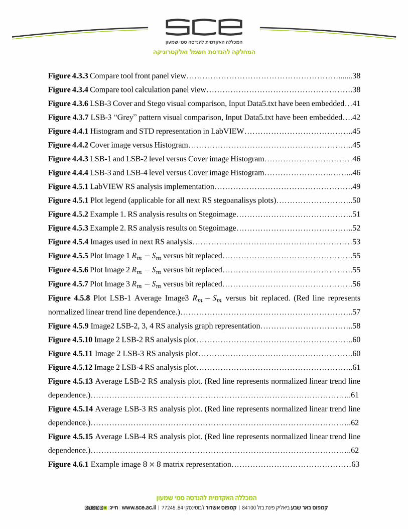
The perfect example of disorientation of Human eye this is Herman Grid presented in Figure 2.4.4.
The intensity at a point in the visual system is not simply the result of a single receptor, but the
result of a group of receptors which respond to the presentation of stimuli in what is called a
receptive field.
המחלקה להנדסת חשמל ואלקטרוניקה
11
Figure 2.4.4 Herman Grid
The most of high quality stegaalgorithms are use Human eye properties are listed above. Usage of
these properties helps to avoid stegoimage visual detection and as result of this the stegoimage
can’t be attacked by digital Steganalysis.
2.5 Classification of Steganography Categories [6].
Steganography is classified into 3 categories:
Pure steganography where there is no stego- key. It is based on the assumption that no other
party is aware of the communication;
Secret key steganography where the stego key is exchanged prior to communication. This
is most susceptible to interception;
Public key steganography where a public key and a private key is used for secure
communication;

המחלקה להנדסת חשמל ואלקטרוניקה
12
2.6 Classification of Steganography Methods [6].
Substitution methods substitute redundant parts of a cover with a secret message (spatial
domain);
Transform domain techniques embed secret information in a transform space of the signal
(frequency domain);
Spread spectrum techniques adopt ideas from spread spectrum communication;
Statistical methods encode information by changing several statistical properties of a cover
and use hypothesis testing in the extraction process;
Distortion techniques store information by signal distortion and measure the deviation from
the original cover in the decoding step;
Cover generation methods encode information in the way a cover for secret communication
is created;
2.6.1 Substitution methods substitute redundant parts of a cover with a secret message (spatial
domain).
These techniques use the pixel gray levels and their color values directly for encoding the message
bits. These techniques are some of the simplest schemes in terms of embedding and extraction
complexity. The major drawback of these methods is amount of additive noise that creeps in the
image which directly affects the Peak Signal to Noise Ratio and the statistical properties of the
image.
One of the common and popular data hiding methods is based on manipulating the Least
Significant Bit (LSB) planes, by direct replacing the LSB’s of the pixel value of the cover image
with the secret message bits. This is the simplest of the digital steganography methods and good
example for explain the main idea behind the bit manipulating theory. The imbedding process
consists of the sequential substitution of each LSB of image pixel for the bit message.

המחלקה להנדסת חשמל ואלקטרוניקה
13
2.6.2 Transform domain techniques embed secret information in a transform space of the signal
(frequency domain):
These techniques try to encode message bits in the transform domain coefficients of the image.
Data embedding performed in the transform domain is widely used for robust watermarking.
Similar techniques can also realize large capacity embedding for steganography. Candidate
transforms include discrete cosine Transform (DCT), discrete wavelet transform (DWT), and
discrete Fourier transform (DFT). By being embedded in the transform domain, the hidden data
resides in more robust areas, spread across the entire image, and provides better resistance against
signal processing.
2.6.3 Spread spectrum techniques adopt ideas from spread spectrum communication:
Spread-spectrum communication describes the process of spreading the bandwidth of a
narrowband signal across a wide band of frequencies. This can be accomplished by modulating
the narrowband waveform with a wideband waveform, such as white noise. After spreading, the
energy of the narrowband signal in any one frequency band is low and therefore difficult to detect.
In these techniques typically uses a binary signal, within very low power white Gaussian noise.
The resulting signal, perceived as noise, is then combined with the cover image to produce the
stegoimage.
2.6.4 Statistical methods encode information by changing several statistical properties of a cover
and use hypothesis testing in the extraction process:
Statistical methods for hiding information based on altering some statistical properties of the
image. They are based on verification of statistical hypotheses. The idea of this method is to change
statistical pattern of the image in manner, whereby received side only can to distinguish modified
image from not modified.

המחלקה להנדסת חשמל ואלקטרוניקה
14
2.6.5 Distortion techniques store information by signal distortion and measure the deviation from
the original cover in the decoding step:
Distortion techniques require the knowledge of the original cover in the decoding process.
Embedding scheme is based on consistent cover image modification by using pseudorandom bits
permutations. The sender first choses 𝐿(𝑚) different cover-pixels he wants to use for information
transfer. Such a selection can again be done using pseudorandom number generators or
pseudorandom permutations. To encode a 0 in one pixel, the sender leaves the pixel unchanged:
to encode a 1, he adds a random value ∆ 𝑋 to the pixel’s color. Although this approach is similar
to a substitution system, there is one significant difference: the LSB of the selected color values
do not necessarily equal secret message bits. In particular, no cover modifications are needed when
coding 0. Furthermore, ∆ 𝑋 can be chosen in a way that better preserves the cover’s statistical
properties.
2.6.6 Cover generation methods encode information in the way a cover for secret communication
is created:
In contrast to all embedding methods presented above, where secret information is added to a
specific cover by applying an embedding algorithm, some steganographic applications generate a
digital object only for the purpose of being a cover for secret communication.
2.7 Classification of Steganalysis Categories [6].
Normally, Steganalysis can be dividing into two main categories:
Visual Attacks
Statistical Attacks
The next Figure 2.7.1 provides visual scheme of Steganalysis hierarchy. Every analysis starts with
visual inspection, only then the steganalyst decides to continue with complicated analysis or not.

המחלקה להנדסת חשמל ואלקטרוניקה
15
Figure 2.7.1 The hierarchy of the classification of Steganalysis techniques.
2.8 Classification of Steganalysis Methods and Techniques [4], [6].
2.8.1 Visual Attacks.
Steganalysis by visual attack was used early in Steganalysis research. The idea of visual attacks is
to remove any parts of the image that cover the message in order for the human eye to distinguish
where there is any hidden message or still image content. An example for sequential embedding
can be to extract the LSB plane of the image and check for any possible suspicious structure in the
image. The LSB plane of a natural grayscale image can be seen in Figure 2.8.1, where it is clear
that there are not any suspicious structures, while viewing the LSB plane of a Stego made with

המחלקה להנדסת חשמל ואלקטרוניקה
16
sequential embedding we can see some sort of structure on the left-most part which can lead to
further investigation in the image.
Natural image Stegoimage
Figure 2.8.1 Grayscale image visual attack example.
Another more technical way to make a visual attack is to apply specific filters on the image and compare it
with a known natural image filtered with same filter, like displayed in Figure 2.8.2.
Natural image filtered Stegoimage filtered
Figure 2.8.2 Grayscale image filter visual attack example.
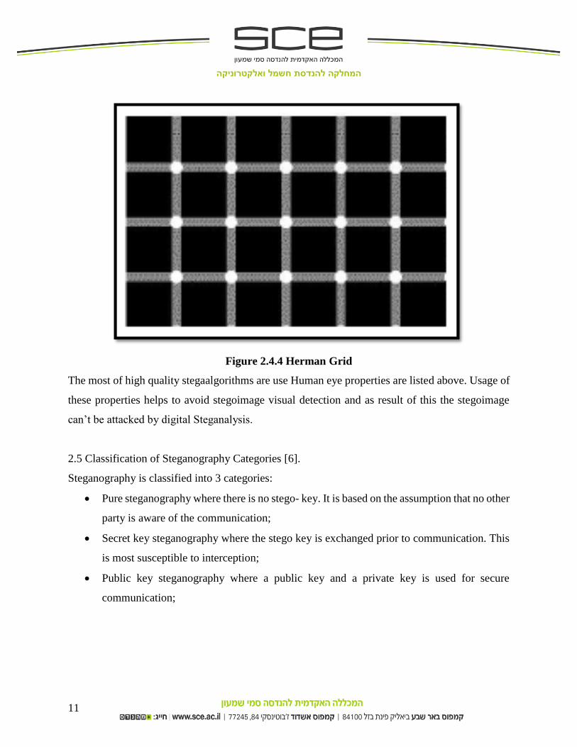
2.8.2 Histogram Analysis Attack.
Histograms analysis attack works on JPEG sequential and pseudo-random embedding type stegosystems.
It can effectively estimate the length of the message embedded and it is based on the loss of histogram
symmetry after embedding. Figure 2.8.3 is displays comparison of natural and stegoimage histograms.
המחלקה להנדסת חשמל ואלקטרוניקה
17
Natural image Natural image histogram Stegoimage histogram
Figure 2.8.3 Grayscale image Cover image versus Stegoimage histogram.
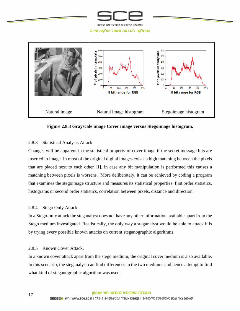
2.8.3 Statistical Analysis Attack.
Changes will be apparent in the statistical property of cover image if the secret message bits are
inserted in image. In most of the original digital images exists a high matching between the pixels
that are placed next to each other [1], in case any bit manipulation is performed this causes a
matching between pixels is worsens. More deliberately, it can be achieved by coding a program
that examines the stegoimage structure and measures its statistical properties: first order statistics,
histograms or second order statistics, correlation between pixels, distance and direction.
2.8.4 Stego Only Attack.
In a Stego-only attack the steganalyst does not have any other information available apart from the
Stego medium investigated. Realistically, the only way a steganalyst would be able to attack it is
by trying every possible known attacks on current steganographic algorithms.
2.8.5 Known Cover Attack.
In a known cover attack apart from the stego medium, the original cover medium is also available.
In this scenario, the steganalyst can find differences in the two mediums and hence attempt to find
what kind of steganographic algorithm was used.

המחלקה להנדסת חשמל ואלקטרוניקה
18
2.8.6 Known Message Attack.
A known message attack can be used when the hidden message is revealed. The steganalyst by
knowing the hidden message can attempt to analyze the Stegoimage for future attacks. Even by
knowing the message, this may be very difficult and may even be considered equivalent to the
Stego-only attack.
2.8.7 Blind Steganalysis.
Technique is designed to work on all types of embedding techniques and image formats. In a few
words, a blind Steganalysis algorithm ‘learns’ the difference in the statistical properties of pure
and Stego images and distinguish between them. The ‘learning’ process is done by training the
machine on a large image database. Blind techniques are usually less accurate than targeted ones,
but a lot more expandable.
2.8.8 Semi-blind.
Technique Steganalysis works on a specific range of different Stego-systems. The range of the
Stego-systems can depend on the domain they embed on, i.e. spatial or transform.
2.9 RS Steganalysis algorithm [1].
Among the methods, the RS Steganalysis algorithm proposed by Fridrich [1], is considered as the
most reliable and accurate method to detect LSB replacing and other bit manipulation
steganography. Fridrich et al. propose a statistical method that uses high order statistics.
This algorithm is worked with regular and singular groups to measure relationship of pixels.
LSB replacement violates the proportion between regular and singular groups and the existence of
the steganography is detected, the secret message length can be estimated by the amount of regular
and singular groups.
In current work RS method is used like reference to prove the viability of proposed improved
Genetic Shifting Algorithm.

המחלקה להנדסת חשמל ואלקטרוניקה
19
According to Fridrich method the image is partitioned into not overlapping groups of a fixed shape.
The LSB embedding increase the noisiness in the image, and thus expects that the value of
discrimination function 𝑓 to increase after LSB embedding. The LSB embedding process
described using flipping functions 𝐹1𝑎𝑛𝑑 𝐹−1.
Positive flipping 𝐹1 – transformation relationship between 2𝑖 𝑎𝑛𝑑 (2𝑖 + 1) (0-1, 2-3… 254-255).
Negative flipping 𝐹−1 – transformation relationship between (2𝑖 − 1)𝑎𝑛𝑑 2𝑖 (-1-0, 1-2… 255-
256).
None flipping 𝐹0.
The relationship between two flipping according to equation 2.9.1
(2.9.1) 𝐹−1 = 𝐹1(𝑥 + 1) − 1
Define 𝐹0 according to equation 2.9.2
(2.9.2) 𝐹1(𝑥) = 𝑥
Now we are can define flipping group – applying flipping function on pixels of image block,
according to 2.9.3.
(2.9.3) 𝐹(𝐺) = (𝐹𝑀(1)(𝑥1), 𝐹𝑀(2)(𝑥2), … 𝐹𝑀(𝑛)(𝑥𝑛)
Regular and Singular groups subject to the next rules: equations 2.9.4 and 2.9.5
(2.9.4) 𝑓(𝐹(𝐺)) > 𝑓(𝐺)
(2.9.5) 𝑓(𝐹(𝐺)) < 𝑓(𝐺)
The discrimination function 𝑓and the flipping operation 𝐹 define three types of pixel groups. By
using concept of shifted LSB flipping or negative mask applying. Each group is classified as

המחלקה להנדסת חשמל ואלקטרוניקה
20
“regular” ,“singular” or “unchanged” depending on whether the pixel noise within the group is
increased or decreased after flipping the LSB’s of fixed set pixels within each group (the pattern
of pixels to flip is called the “mask” M). The classification is repeated for a dual type of flipping.
Some theoretical analysis and some experimentation show that the proportion of regular and
singular groups form curves quadratic in the amount of message embedded by the LSB method.
Under a similar assumption to above, this time about the proportions of regular and singular groups
with respect to the standard and dual flipping, sufficient information can be gained to estimate the
proportion of an image in which data is hidden. Statistically tested that applying flipping on typical
image total number of “Regular” groups will be larger than the total number of “Singular” groups.
For positive flipping, denote the number of Regular groups for mask 𝑀 as 𝑅𝑚 (in percents of all
groups). Similarly, 𝑆𝑚 will denote the number of Singular groups. In the same way 𝑅−𝑚 and 𝑆−𝑚
are defined as the number of Regular and Singular blocks after the negative flipping.
In case embedding “zero” message in typical cover image 𝑅𝑚 is approximately equal to 𝑅−𝑚, and
the same should be true for 𝑆𝑚 and 𝑆−𝑚.
According to Fridrich statistically analysis permutations in LSB plane forces the difference
between 𝑅𝑚 and 𝑆𝑚 to zero as the length m of the embedded message increases. Another words,
after flipping some quantity of LSB we obtain result 𝑅𝑚 ≈ 𝑆𝑚. But this applies opposite effect on
𝑅−𝑚 and 𝑆−𝑚 components- their difference increases with the length m of imbedded message.
The principle of Fridrich steganalytic method, which called RS Steganalysis, is to estimate the four
curves of the RS diagram and calculate their intersection using extrapolation. Fridrich collected
experimental evidence that the 𝑅−𝑚 and 𝑆−𝑚curves are well modeled with straight lines, while
second-degree polynomials can approximate the “inner” curves 𝑅−𝑚 and 𝑆−𝑚 reasonably well.
Statistical data accumulated by Fridrich is presented in Figure 2.9.1.

המחלקה להנדסת חשמל ואלקטרוניקה
21
Figure 2.9.1 RS-diagram of an image taken by a digital camera. The X-axis is the
percentage of pixels with flipped LSBs, the Y-axis is the relative number of regular and
singular groups with mask M.
2.10 Genetic Shifting algorithm (GSM) [2].
Shen Wang and al [2], propose new “Genetic” based algorithm in which the existence of the secret
message is hard to be detected by the RS analysis [1]. And better visual quality of stegoimage can
be achieved by this steganography method. The main idea of Genetic algorithm to search for a best
adjustment matrix. Genetic algorithm is a general optimization algorithm. After secret message is
embedded and stegoimage is received the type (regular or singular) of the block can be changed
by a proper adjustment. Pixel adjustment of stegoimage is performed to make 𝑅𝑚 ≈ 𝑆𝑚, 𝑅−𝑚 ≈
𝑆−𝑚 and keep image statistic characteristics. Hence, the RS analysis cannot detect the existence
of the stegomessage. This is method was used as the base for current work. But main disadvantage
of proposed method is performing manipulation on the stego and not on the original image. In this
case adjustment matrix (secret key) should be transmitted with every image.

המחלקה להנדסת חשמל ואלקטרוניקה
22
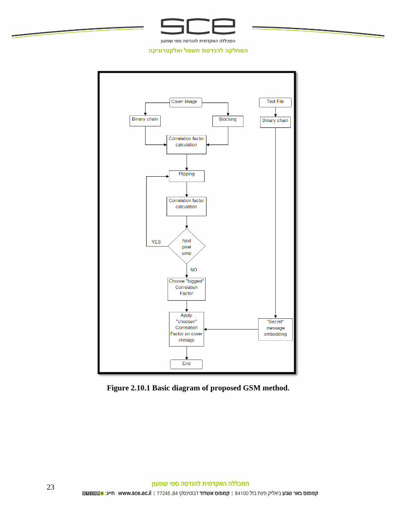
2.10.1 Steps of GSM.
Perform operations same to regular LSB method: convert cover image to binary numbers
chain.
In next step perform “Correlation Factor” calculation of original image, by equation 2.10.1.
(2.10.1)
𝐶 = ∑(𝑖 + 1) − 𝑖
𝑁 − 1
𝑁
𝑖
Where 𝑁 – this is number of pixels, and (𝑖 + 1) and 𝑖 are indicate current and next pixel
values.
After the first Correlation Factor is calculated apply non-positive flipping 𝐹− and no-negative
flipping 𝐹+ on first pixel of original image binary chain.
Perform Correlation Factor calculation for these new values, according to formula (6.1)
Move to the next pixel and perform step 4 again.
Continue to calculate Correlation Factors till last pixel of the original image.
Need to choose biggest value of Correlation Factor from all Correlation Factors are calculates
in previous steps and adjust original image according to this value.
For example, original cover image consist of three pixels, calculate Correlation Factors by using
equation 2.10.1. The result is four Correlation factors equation 2.10.2, where 𝐶0 is Correlation
Factor for original binary chine and 𝐶1𝐶2𝐶3 values for other pixels.
(2.10.2) 𝐶0𝐶1𝐶2𝐶3
Choose the biggest value from the result and apply on the original image. After that LSB
manipulation can be performed. See Figure 2.10.1 for diagram of Shen Wang [2] GSM method.
המחלקה להנדסת חשמל ואלקטרוניקה
23
Figure 2.10.1 Basic diagram of proposed GSM method.

המחלקה להנדסת חשמל ואלקטרוניקה
24
3. Description and system requirements.
3.1 Program interface.
Main Directory – Steganography, Figure 3.1.1;
Cover Images – list of images to run though;
Input files – text messages with different length for simulation;
Output files – recovered messages;
Stegoimage – images with embedded message;
New_Encoding+Decoding_RGB.vi– code/decode/extract message and perform RS/GSM with 1D
array representation;
Figure 3.1.1 “Steganography” directory view.

המחלקה להנדסת חשמל ואלקטרוניקה
25
3.2 Front panel view.
Figure 3.2.1 displayed program front panel view.
Figure 3.2.1 Detailed program front panel view.
1. Source cover image;
2. Result stegoimage;
3. Cover Histogram and STD statistic window;
4. Stegoimage Histogram and STD statistic window;
5. RS analysis results on Stegoimage;
6. LSB level to be used (up to LSB-4);
7. Start shifting (GSM);
8. Standard deviation evaluation;
9. Snaked array length;
10. Open output result text message;
11. Decode message from stegoimage;
12. Encode message into cover message;
13. Stop button;
14. Start / stop menu;

המחלקה להנדסת חשמל ואלקטרוניקה
26
3.3 Steps for basic encoding and decoding procedure of images.
1. Load “Encoding / Decoding” dashboard, presented in Figure 3.3.1
Figure 3.3.1 “Encoding / Decoding” dashboard view
2. Choose number of LSB bits included in embedding message into image, by using “Bits
Embedded” up/down button.
3. Choose Shifted array length by using “Division of shifted array” toggle.
4. Pushing “Encode” button will start Encoding process. The encoding process - this is
embedding messages from “Input files” Figure 3.3.2, directory into images preloaded to
“Cover Images” directory, Figure 3.3.3.

המחלקה להנדסת חשמל ואלקטרוניקה
27
Figure 3.3.2 “Input files” directory view
Figure 3.3.3“Cover Images” directory view
Input text files have different size to learn statistical and visual degradation of images after
message embedding. Encoding process generate seven “Stego” images, for every encoding image
- product of different message size embedded, in the “Stego images” directory, see Figure 3.3.4.
First text file have zero value and required to design RS analysis graphical and statistical
representation

המחלקה להנדסת חשמל ואלקטרוניקה
28
Figure 3.3.4 Resulting “Stegoimage” directory view
Every stegoimage presented in “Stegoimages” directory have different message size imbedded
inside. Image ending with Data5 have maximum message length and have ending Data have zero
message imbedded respectively.
5. To start the recovery of message from “Stego” image need to push “Decode” button. This
action is open window for choosing specific image for text recovery. This process is
presented in Figure 3.3.5.

המחלקה להנדסת חשמל ואלקטרוניקה
29
Figure 3.3.5 message recovery process.
User sign the required image and press “OK” button after thereafter.
6. Pressing “Open output” button will open recovered text message, Figure 3.3.6.
Figure 3.3.6 Resulting recovered message view.
The output message size depends of original image size, LSB number and input message size.

המחלקה להנדסת חשמל ואלקטרוניקה
30
3.4 LSB steganography steps.
1. Convert the secret data (message that will be imbedded in to cover image) to binary form.
2. Read cover image and convert decimal form of the cover image to binary form.
3. Replace of Least Significant Bit of image with bits from a message by using LSB encoder.
4. Repeat previous operation many times as needed to imbed the all message in to the image.
5. After manipulating with LSB is done and all message inserted in to the cover image convert
the new binary matrix back to decimal form and to a pixels.
6. The new image which is obtained after this process is named “Stego- image”.
Figure 3.4.1 LSB steps.
המחלקה להנדסת חשמל ואלקטרוניקה
31
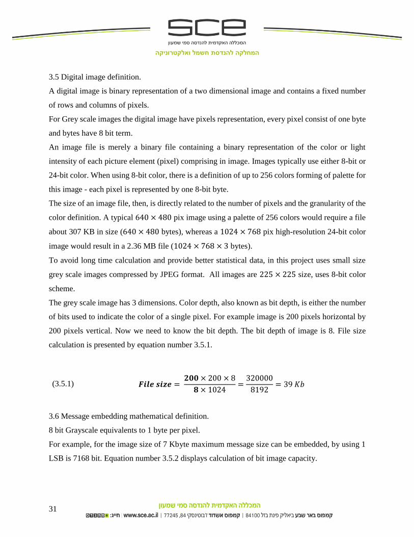
3.5 Digital image definition.
A digital image is binary representation of a two dimensional image and contains a fixed number
of rows and columns of pixels.
For Grey scale images the digital image have pixels representation, every pixel consist of one byte
and bytes have 8 bit term.
An image file is merely a binary file containing a binary representation of the color or light
intensity of each picture element (pixel) comprising in image. Images typically use either 8-bit or
24-bit color. When using 8-bit color, there is a definition of up to 256 colors forming of palette for
this image - each pixel is represented by one 8-bit byte.
The size of an image file, then, is directly related to the number of pixels and the granularity of the
color definition. A typical 640 × 480 pix image using a palette of 256 colors would require a file
about 307 KB in size (640 × 480 bytes), whereas a 1024 × 768 pix high-resolution 24-bit color
image would result in a 2.36 MB file (1024 × 768 × 3 bytes).
To avoid long time calculation and provide better statistical data, in this project uses small size
grey scale images compressed by JPEG format. All images are 225 × 225 size, uses 8-bit color
scheme.
The grey scale image has 3 dimensions. Color depth, also known as bit depth, is either the number
of bits used to indicate the color of a single pixel. For example image is 200 pixels horizontal by
200 pixels vertical. Now we need to know the bit depth. The bit depth of image is 8. File size
calculation is presented by equation number 3.5.1.
3.6 Message embedding mathematical definition.
8 bit Grayscale equivalents to 1 byte per pixel.
For example, for the image size of 7 Kbyte maximum message size can be embedded, by using 1
LSB is 7168 bit. Equation number 3.5.2 displays calculation of bit image capacity.
(3.5.1)
𝑭𝒊𝒍𝒆 𝒔𝒊𝒛𝒆 = 𝟐𝟎𝟎 × 200 × 8
𝟖 × 1024=
320000
8192= 39 𝐾𝑏

המחלקה להנדסת חשמל ואלקטרוניקה
32
(3.5.2) 7 𝐾𝑏 × 1024 = 7168 𝑏𝑦𝑡𝑒𝑠
7168 𝑏𝑦𝑡𝑒𝑠 × 8 𝑏𝑖𝑡 = 57344 𝑏𝑖𝑡
We are replacer one bit in every byte. In case we are try to embed message larger than maximum
image capacity the message will be cut, and part of information will be lost.
Table number 3.6.1 demonstrate maximum possible embedded message capacity as function of
LSB level to be used in same image size.
LSB level Maximum message size
1 7 Kb
2 14 Kb
3 21 Kb
4 28 Kb
Table 3.6.1 capacity as function of LSB level.

המחלקה להנדסת חשמל ואלקטרוניקה
33
4. Steps of experiment, discussion and definition.
4.1 Steps definition.
All experiments and research to be performed in LabVIEW environment.
1. Build LabVIEW based steganography system.
2. Perform basic message coding (Cover Image) up to LSB-4 for gray images.
3. Perform basic message recovery (Stegoimages) up to LSB-4 for gray images.
4. Compare visual image degradation.
5. Compare visual degradation through common tools (Histogram, STD).
6. Perform study of coded message saturation (message of different length) vs. recovery and
image degradation per different LSB coding at gray images.
7. Build RS analysis (Fridrich algorithm) routine.
8. Confirm validity of RS analysis on gray images.
9. Implement secure genetic steganography method for RS baseline shifting for LSB-1. (GSM
for RS shifting).
10. Perform basic message recovery with GSM for RS shifting for LSB-1.
11. Perform RS analysis comparison for different message length with GSM for RS shifting
and without, use different “snake” division array image representation.
12. Conclusion.
4.2 Build LabVIEW based steganography system.
Next Figures 4.2.1 and 4.2.2 are displays most important parts of steganography system block
diagram.

המחלקה להנדסת חשמל ואלקטרוניקה
34
Figure 4.2.1 Program block diagram view.
Figure 4.2.2 Detailed Program block diagram view.

המחלקה להנדסת חשמל ואלקטרוניקה
35
Two loops chosen for taking images and messages permutation.
First step – open image.
Same time we could perform math analysis and RS analysis of the image without message.
In case if we need to mask RS dependency we could press.
Next we start to open shortest message, convert it from ASCII to Int U8 in binary code.
Next step we are interleaving image with message – for 1LSB image opens to 1D array,
for 2LSB to 2D array and so on. Every image byte consequently getting be changed by
value of message bit (1 bit in byte for 1 LSB 2 bits in byte for 2LSB and so on) – by this
getting the stegoimage.
After receiving of stegoimage we run math analysis and RS analysis of the image with
message.
RS and Math analysis will be displayed.
In text (inner) loop we are taking same image, but longer message.
All the process will repeat itself.
After we use all the messages, we going to the next image in directory and all the process
come back until we will not use all the images and messages.
4.3 Perform basic message coding and recovery. Compare visual image degradation.
Visual Attacks are widely regarded as the simplest form of Steganalysis. A visual attack largely
involves examining the subject file with the naked eye to identify any obvious inconsistencies.
4.3.1 Perform LSB-1 coding.
Prepare six messages of different length to be embed in to images, according to table 4.3.1:
Input Data.txt 0 bytes
Input Data0.txt 699 bytes
Input Data1.txt 2.17 KB (2,225 bytes)
Input Data2.txt 3.95 KB (4,055 bytes)
Input Data3.txt 4.12 KB (4,222 bytes)
Input Data4.txt 4.78 KB (4,896 bytes)
Input Data5.txt 36.0 KB (36,920 bytes)
Table 4.3.1 Used messages sizes.

המחלקה להנדסת חשמל ואלקטרוניקה
36
Also use six different Grey scale images. All images are 225 × 225 𝑝𝑖𝑥𝑒𝑙𝑠 size, uses 8-bit color
scheme. Images have different patterns with different grey scale distributions. One of the images
this is lines pattern of few shadows of grey. This is image provides better visual comparing
capabilities.
Compare Cover (original) image with Stegoimage. Figure 4.3.1 displays visual comparison.
Cover image Stegoimage
Figure 4.3.1 LSB-1 Cover and Stego visual comparison, Input Data5.txt have been
embedded.
No any visual degradation seen, even if zoom in to both images.
In next step try to recover message from Stegoimage. The recovered text file size is 6.21 KB (6,361
bytes), 1177 words text, equivalent to 2.5 pages in WORD format. We can see that by using 1LSB
level only possibly to embed enough amount of information in relatively small image.
Perform similar comparison of special “Grey scale” pattern, Figure 4.3.2:

המחלקה להנדסת חשמל ואלקטרוניקה
37
Cover image Stegoimage
Figure 4.3.2 1LSB “Grey” pattern, Input Data5.txt have been embedded.
The result is same – no any visual image degradation.
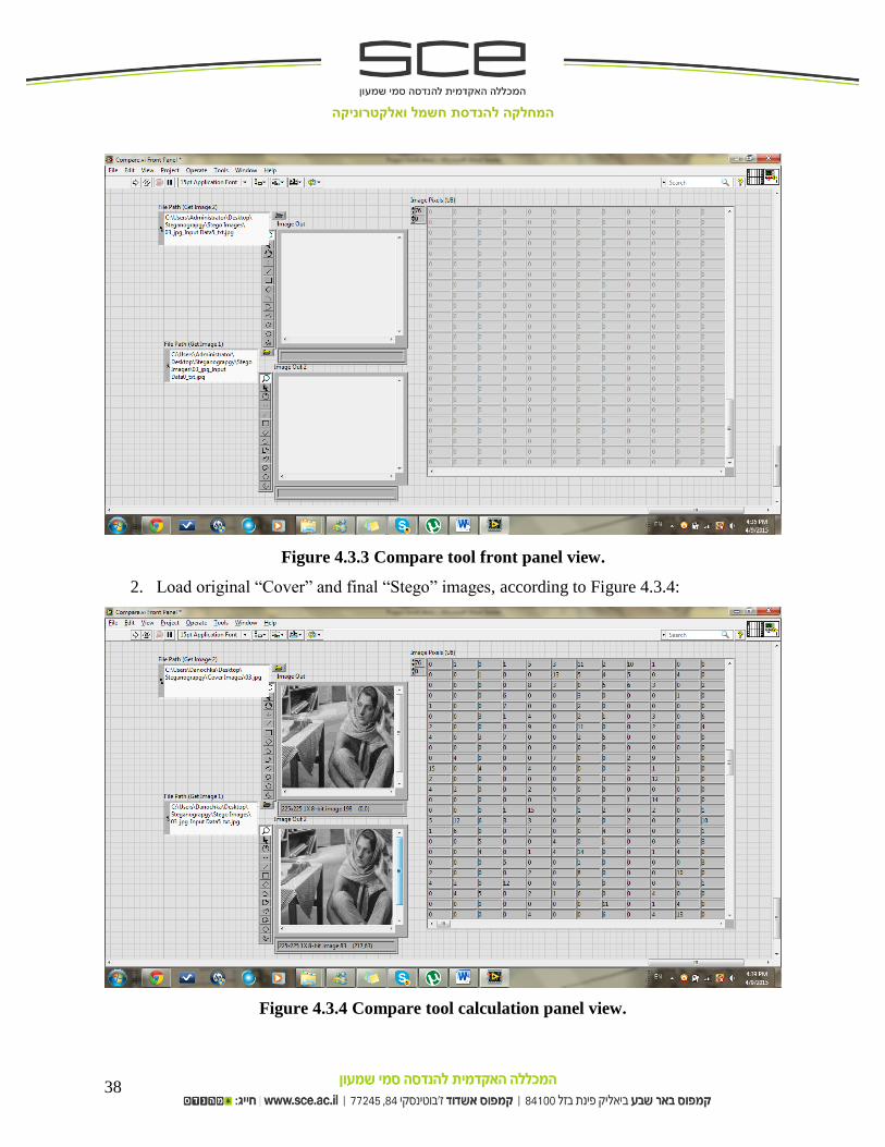
4.3.2 Comparing tool.
Prepare comparing tool, LabVIEW based also, to validate message embedding in to image. The
function of the comparing tool is calculating the difference between bit matrices of Cover image
and bit matrices of Stego Image to determinate percentage of pixels permutations.
The comparing procedure is simple:
1. Open comparing LabVIEW based tool.
Figure 4.3.3 is displayed Comparing tool front panel.
המחלקה להנדסת חשמל ואלקטרוניקה
38
Figure 4.3.3 Compare tool front panel view.
2. Load original “Cover” and final “Stego” images, according to Figure 4.3.4:
Figure 4.3.4 Compare tool calculation panel view.

המחלקה להנדסת חשמל ואלקטרוניקה
39
The number in matrix is shows bits difference between two images. Zero, denotes no differences.
For example, take small part of the compare matrix of “Gray scale” image, presented in Tables
4.3.2 and 4.3.3.
67 70 55 88 96 80 121 98
91 73 56 73 81 42 80 80
108 104 58 108 80 80 59 79
78 100 64 128 105 131 73 78
61 78 93 119 146 126 109 103
72 79 89 120 129 97 113 132
81 81 49 101 79 73 92 109
100 86 48 76 85 76 109 78
Table 4.3.2 Cover image pixel matrix.
66 71 55 88 96 80 121 98
90 72 56 72 81 42 80 81
109 104 59 109 81 80 58 79
79 100 65 129 104 131 72 78
60 79 93 118 146 127 108 102
73 79 88 121 129 96 112 132
80 80 48 100 78 72 92 109
100 86 48 76 84 76 109 78
Table 4.3.3 Stegoimage pixel matrix.
From Table 4.3.4 can see, that not every pixel has been changed.
0 1 0 0 0 0 0 0
0 0 0 0 0 0 0 1
1 0 1 1 1 0 0 0
1 0 1 1 0 0 0 0
0 1 0 0 0 1 0 0
1 0 0 1 0 0 0 0
0 0 0 0 0 0 0 0
0 0 0 0 0 0 0 0
Table 4.3.4 Difference image pixel matrix.
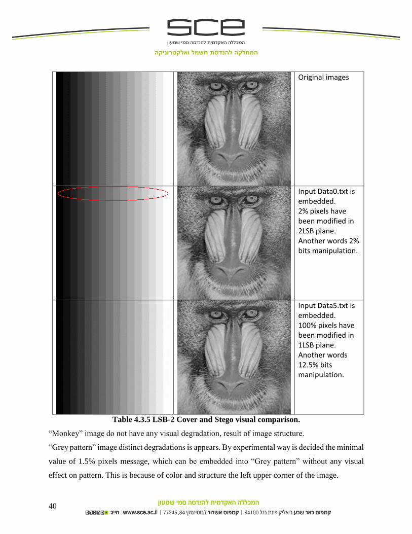
4.3.3 Perform LSB-2 coding.
Use scheme of experiment is analog to LSB-1 coding. Table 4.3.5 provide us by Cover and
Stego visual comparison results.
המחלקה להנדסת חשמל ואלקטרוניקה
40
Original images
Input Data0.txt is embedded. 2% pixels have been modified in 2LSB plane. Another words 2% bits manipulation.
Input Data5.txt is embedded. 100% pixels have been modified in 1LSB plane. Another words 12.5% bits manipulation.
Table 4.3.5 LSB-2 Cover and Stego visual comparison.
“Monkey” image do not have any visual degradation, result of image structure.
“Grey pattern” image distinct degradations is appears. By experimental way is decided the minimal
value of 1.5% pixels message, which can be embedded into “Grey pattern” without any visual
effect on pattern. This is because of color and structure the left upper corner of the image.
המחלקה להנדסת חשמל ואלקטרוניקה
41
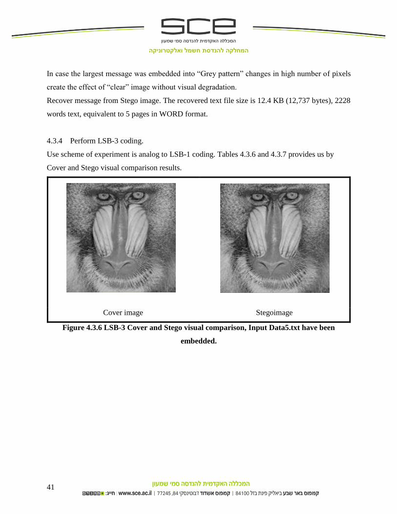
In case the largest message was embedded into “Grey pattern” changes in high number of pixels
create the effect of “clear” image without visual degradation.
Recover message from Stego image. The recovered text file size is 12.4 KB (12,737 bytes), 2228
words text, equivalent to 5 pages in WORD format.
4.3.4 Perform LSB-3 coding.
Use scheme of experiment is analog to LSB-1 coding. Tables 4.3.6 and 4.3.7 provides us by
Cover and Stego visual comparison results.
Cover image Stegoimage
Figure 4.3.6 LSB-3 Cover and Stego visual comparison, Input Data5.txt have been
embedded.
המחלקה להנדסת חשמל ואלקטרוניקה
42
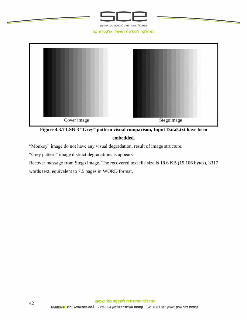
Cover image Stegoimage
Figure 4.3.7 LSB-3 “Grey” pattern visual comparison, Input Data5.txt have been
embedded.
“Monkey” image do not have any visual degradation, result of image structure.
“Grey pattern” image distinct degradations is appears.
Recover message from Stego image. The recovered text file size is 18.6 KB (19,106 bytes), 3317
words text, equivalent to 7.5 pages in WORD format.

המחלקה להנדסת חשמל ואלקטרוניקה
43
4.3.5 Perform LSB-4 coding
Use scheme of experiment is analog to LSB-1 coding. Table 4.3.8 provide us by Cover and
Stego visual comparison results.
Original images
Input Data4.txt is embedded. 8% pixels have been modified in 4LSB plane. Another words 4.3% bits manipulation.
Input Data5.txt is embedded. 100% pixels have been modified in 4LSB plane. Another words 50% bits manipulation.
Table 4.3.8 LSB-4 Cover and Stego visual comparison.
Both of the images have distinct degradation after LSB-4 manipulation.

המחלקה להנדסת חשמל ואלקטרוניקה
44
Recover message from Stego image. The recovered text file size is 24.8 KB (25,477 bytes), 4468
words text, equivalent to 10 pages in WORD format – this is a maximum text file size can be
imbedded into 225 × 225 𝑝𝑖𝑥𝑒𝑙𝑠 image by using 4LSB plane.
4.3.6 Intermediates conclusions.
Image color and structure have important value in steganography process. One tone images are
unsuitable for steganography, due to high sensitivity to bits manipulation – high statistical
dependence between closed pixels. Opposite, images with more small details, wide spectrum of
shadows and with structural margins are ideal candidates for steganography, even high LSB levels
and large messages use.
4.4 Compare visual degradation through common tools (Histogram, STD).
4.4.1 Histogram.
“Image histogram, is a type of histogram that acts as a graphical representation of the tonal
distribution in digital image. It plots the number of pixels for each tonal value. By looking at the
histogram for a specific image a viewer will be abble to judge the entire tonal distribution. The
horisontal axis of the graph represents the tonal variations, while the verticalaxis represents the
number of pixels in that particular tone. The left side of the horisontal axis represents the black
areas, the middle represents medium grey and the right hand side represents pure white areas.
Thus, the istogramm for a very dark image will have the majority of its data points on the left side
and sentre og graph. Conversely, the histogram for a very bright image with few dark areas will
have most of its ata points on the right side and centre of the graph.
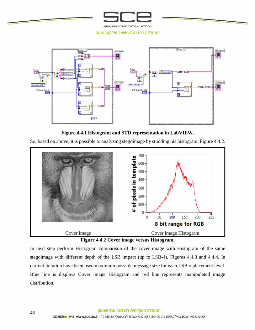
So, based on above, it is possible to analising stego image by studing his histogram. LabVIEW
Histogram and STD representation demonstrated in Figure 4.4.1.
Compare Histogram of the cover image with Histogram of the same stegoimage by with different
depth of the LSB impact. In current iteration have been used maximum possible message size for
each LSB replacement level.
המחלקה להנדסת חשמל ואלקטרוניקה
45
Figure 4.4.1 Histogram and STD representation in LabVIEW.
So, based on above, it is possible to analyzing stegoimage by studding his histogram, Figure 4.4.2.
Cover image Cover image Histogram
Figure 4.4.2 Cover image versus Histogram.
In next step perform Histogram comparison of the cover image with Histogram of the same
stegoimage with different depth of the LSB impact (up to LSB-4), Figures 4.4.3 and 4.4.4. In
current iteration have been used maximum possible message size for each LSB replacement level.
Blue line is displays Cover image Histogram and red line represents manipulated image
distribution.

המחלקה להנדסת חשמל ואלקטרוניקה
46
1LSB level 2LSB level
Figure 4.4.3 LSB-1 and LSB-2 level versus Cover image Histogram.
3LSB level 4LSB level
Figure 4.4.4 LSB-3 and LSB-4 level versus Cover image Histogram.
Next Table 4.4.1 can us to see “how” stegoimage Histogram is depredate in dependence of input
message volume.

המחלקה להנדסת חשמל ואלקטרוניקה
47
No message inside 4LSB level 699 bytes message
4LSB level 2,225 bytes message 4LSB level 4,055 bytes message
4LSB level 4,222 bytes message 4LSB level 6,201 bytes message
4LSB level 25,477 bytes message
Table 4.4.1 Histogram degradation trough of message enlargement for LSB-4 level.
STD degradation of Stegoimage in dependence of LSB level is presented in Table 4.4.2.

המחלקה להנדסת חשמל ואלקטרוניקה
48
Cover image Cover image STD
1LSB level 2LSB level
3LSB level 4LSB level Table 4.4.2 STD graph degradation trough of LSB level increase.

המחלקה להנדסת חשמל ואלקטרוניקה
49
4.4.2 Intermediates conclusions.
In most of the original digital images exists a high matching between the pixels that are placed
next to each other [1], in case any bit manipulation is performed this causes a matching between
pixels is worsens. This is reason for high histogram sensitive for any bits replacements.
But in same time, we can see, that 1LSB level do not dramaticaly impact image histigram, and in
case no clean image histogram presents to cmpare, this is immposible to determinate stegomesage
is exists. In turn, have low sensitivity to LSB permutations and up to 3LSB can’t to provide exact
information according to message presents.
4.5 RS analysis (Fridrich algorithm) routine implementation.
4.5.1 Confirm validity of RS analysis on gray images.
Algorithm require transform image to 1D array in snake pattern (snake array).
Apply positive 𝐹1 and negative 𝐹−1 flipping on resulting array.
Evaluate amount of 𝑅𝑚 and 𝑅−𝑚 (regular groups) for positive and negative flipping.
Evaluate amount of 𝑆𝑚 and 𝑆−𝑚 (singular groups) for positive and negative flipping.
𝑅0 𝑎𝑛𝑑 𝑆0 represents Unchanged groups and not used for analysis.
LabVIEW RS analysisand representation demonstrated in Figure 4.5.1, and results plot legend is
presented in Figure 4.5.1.
Figure 4.5.1 LabVIEW RS analysis implementation.
המחלקה להנדסת חשמל ואלקטרוניקה
50
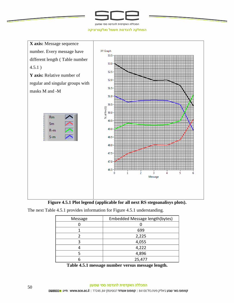
X axis: Message sequence
number. Every message have
different length ( Table number
4.5.1 )
Y axis: Relative number of
regular and singular groups with
masks M and -M
Figure 4.5.1 Plot legend (applicable for all next RS stegoanalisys plots).
The next Table 4.5.1 provides information for Figure 4.5.1 understanding.
Message Embedded Message length(bytes)
0 0
1 699
2 2,225
3 4,055
4 4,222
5 4,896
6 25,477
Table 4.5.1 message number versus message length.

המחלקה להנדסת חשמל ואלקטרוניקה
51
Perform RS analysis according to Fridrich algorithm on our images, use LSB-1 level. RS analyzing
result plot and data are displayed in Figures 4.5.2, 4.5.3 and Tables 4.5.1, 4.5.2.
Just to remember, according to RS algorithm we are expect that 𝑅𝑚 𝑎𝑛𝑑 𝑆𝑚 pair will strive to
equality and 𝑅−𝑚 𝑎𝑛𝑑 𝑆−𝑚 pair will strive to opposite ways.
Figure 4.5.2 Example 1. RS analysis results on Stegoimage.
Message Message length(bytes) % of Rm % of Sm % of R-m % of S-m
0 0 54.9 45.1 49.8 50.2
1 699 53.8 46.2 50.7 49.3
2 2,225 52.1 47.9 52.1 47.9
3 4,055 51.5 48.5 52.6 47.4
4 4,222 51.4 48.6 52.7 47.3
5 4,896 50.8 49.2 53.2 46.8
6 25,477 49.8 50.2 53.8 46.2
Table 4.5.1 Example 1 𝑹𝒎, 𝑺𝒎, 𝑹−𝒎, 𝑺−𝒎 pairs versus message volume.
המחלקה להנדסת חשמל ואלקטרוניקה
52
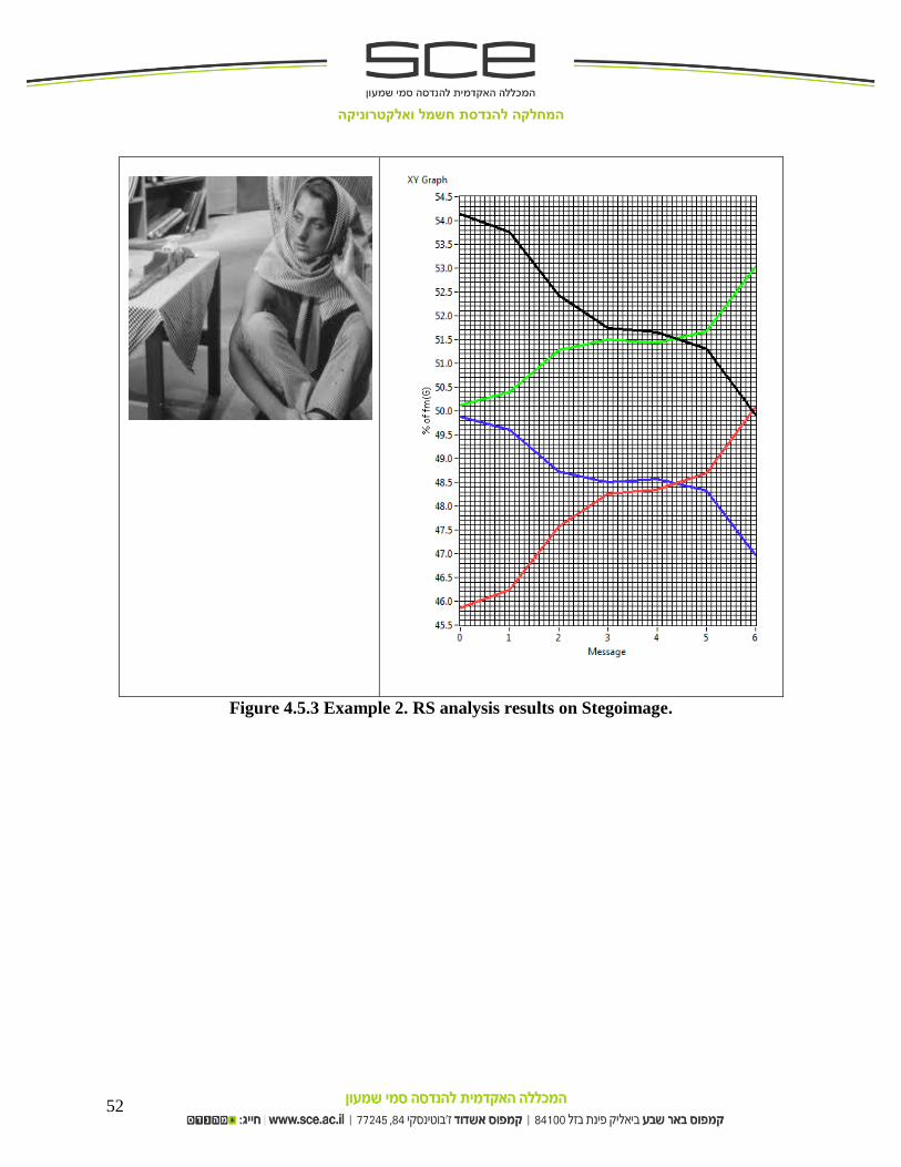
Figure 4.5.3 Example 2. RS analysis results on Stegoimage.

המחלקה להנדסת חשמל ואלקטרוניקה
53
Message Message length(bytes) % of Rm % of Sm % of R-m % of S-m
0 0 54.1 45.9 50.1 49.9
1 699 53.8 46.2 50.4 49.6
2 2,225 52.4 47.6 51.3 48.7
3 4,055 51.7 48.3 51.5 48.5
4 4,222 51.7 48.3 51.4 48.6
5 4,896 51.3 48.7 51.7 48.3
6 25,477 49.9 50.1 53 47
Table 4.5.2 Example 1 𝑹𝒎, 𝑺𝒎, 𝑹−𝒎, 𝑺−𝒎 pairs versus message volume.
For more demonstrative confirmation of this Fridrich postulate, perform statistical analysis of
received data. Analysis of 3 different images from Figure 4.5.4 is present in Table 4.5.3, where
“diff” column represents numerical 𝑅𝑚/𝑆𝑚 differences values for each message length.
Image1 Image 2 Image 3
Figure 4.5.4 Images used in next RS analysis.

המחלקה להנדסת חשמל ואלקטרוניקה
54
Image1
Message % of Rm % of Sm diff
Message length(bytes) % of imager
0 54.9 45.1 9.8 0 0
1 53.8 46.2 7.6 699 1.05
2 52.1 47.9 4.2 2,225 3.35
3 51.5 48.5 3 4,055 6.11
4 51.4 48.6 2.8 4,222 6.36
5 50.8 49.2 1.6 6,201 9.34
6 49.8 50.2 -0.4 8,169 12.3
Image2
0 54.2 45.8 8.4 0 0
1 53.9 46.1 7.8 699 1.78
2 52.5 47.5 5 2,225 5.67
3 51.8 48.2 3.6 4,055 10.34
4 51.7 48.3 3.4 4,222 10.76
5 50 50 0 6,201 15.8
6 49.8 50.2 -0.4 6,361 16.33
Image3
0 52.5 47.5 6 0 0
1 52 48 5 699 1.05
2 51.8 48.2 4.4 2,225 3.35
3 51.9 48.1 4 4,055 6.11
4 51.7 48.3 4 4,222 6.36
5 50.9 49.1 3.4 6,201 9.34
6 50.8 49.2 0.6 8,169 12.31
Table 4.5.3 𝑹𝒎/𝑺𝒎 differences versus message volume.
Only last (largest) message volumes have been increases, according to estimations. By using
previous data we are can to build dependence plots of 𝑅𝑚 and 𝑆𝑚 differences in percent, by
amount of bits are replaced, in percent’s of all image bits. Figures 4.5.5, 4.5.6 and 4.5.7 provide
us by this data.

המחלקה להנדסת חשמל ואלקטרוניקה
55
Figure 4.5.5 Plot Image 1 𝑹𝒎 − 𝑺𝒎 versus bit replaced.
Figure 4.5.6 Plot Image 2 𝑹𝒎 − 𝑺𝒎 versus bit replaced.
המחלקה להנדסת חשמל ואלקטרוניקה
56
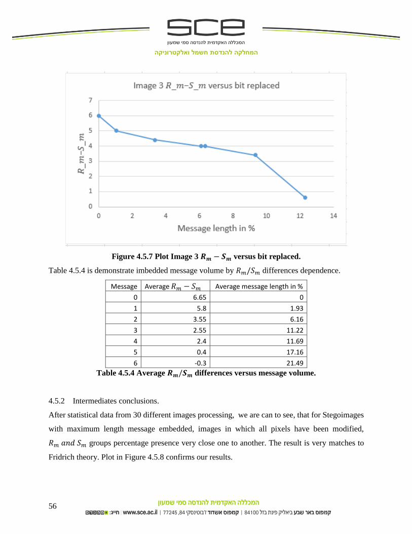
Figure 4.5.7 Plot Image 3 𝑹𝒎 − 𝑺𝒎 versus bit replaced.
Table 4.5.4 is demonstrate imbedded message volume by 𝑅𝑚/𝑆𝑚 differences dependence.
Message Average 𝑅𝑚 − 𝑆𝑚 Average message length in %
0 6.65 0
1 5.8 1.93
2 3.55 6.16
3 2.55 11.22
4 2.4 11.69
5 0.4 17.16
6 -0.3 21.49
Table 4.5.4 Average 𝑹𝒎/𝑺𝒎 differences versus message volume.
4.5.2 Intermediates conclusions.
After statistical data from 30 different images processing, we are can to see, that for Stegoimages
with maximum length message embedded, images in which all pixels have been modified,
𝑅𝑚 𝑎𝑛𝑑 𝑆𝑚 groups percentage presence very close one to another. The result is very matches to
Fridrich theory. Plot in Figure 4.5.8 confirms our results.

המחלקה להנדסת חשמל ואלקטרוניקה
57
Figure 4.5.8 Plot LSB-1 Average Image3 𝑹𝒎 − 𝑺𝒎 versus bit replaced. (Red line represents
normalized linear trend line dependence.).
This is statistical analysis gives us tool to determinate stegamesage presence in the image and
approximate length of presence message. Use presence graphical dependence and know given
image volume we can with high probability determine embedded message existence and
approximate message length. Another words𝑅𝑚 − 𝑆𝑚 differences less 7% indicates LSB
manipulations with high probability.
4.5.3 RS analysis for LSB – 2, 3, 4 levels.
Use Image 2 for example (reference Figure 4.5.4). Figure 4.5.9 and Table 4.5.5 show results of
Image 2 RS analysis for difference LSB levels.

המחלקה להנדסת חשמל ואלקטרוניקה
58
Image 2 LSB-2 RS analysis
LSB-3 RS analysis LSB-4 RS analysis
Figure 4.5.9 Image2 LSB-2, 3, 4 RS analysis graph representation.

המחלקה להנדסת חשמל ואלקטרוניקה
59
2LSB
Message % of Rm % of Sm diff
Message length(bytes)
% of imager
0 54.2 45.8 8.4 0 0
1 54 46 8 699 1.78
2 53.4 46.6 6.8 2,225 5.67
3 52.8 47.2 5.6 4,055 10.34
4 52.7 47.3 5.4 4,222 10.76
5 52.1 47.9 4.2 6,201 15.8
6 50.9 49.1 1.8 12,737 24.31
3LSB
0 54.2 45.8 8.4 0 0
1 54.2 45.8 8.4 699 1.78
2 54.2 45.8 8.4 2,225 5.67
3 53.9 46.1 7.8 4,055 10.34
4 53.9 46.1 7.8 4,222 10.76
5 53.4 46.6 6.8 6,201 15.8
6 52 48 4 19,106 36.47
4LSB
0 54.2 45.8 8.4 0 0
1 54.1 45.9 8.2 699 1.78
2 54 46 8 2,225 5.67
3 53.9 46.1 7.8 4,055 10.34
4 53.9 46.1 7.8 4,222 10.76
5 53.4 46.6 6.8 6,201 15.8
6 50.3 49.7 0.6 25,477 48.56
Table 4.5.5 Image 2 RS analysis results.
Only last (largest) message volumes have been increases, according to estimations. By using
previous data we are can to build dependence plots of 𝑅𝑚 and 𝑆𝑚 differences in percent, by
amount of bits are replaced, in percent’s of all image bits. Figures 4.5.10, 4.5.11 and 4.5.12 provide
us by this data for Image 2 and difference LSB levels.

המחלקה להנדסת חשמל ואלקטרוניקה
60
Figure 4.5.10 Image 2 LSB-2 RS analysis plot.
Figure 4.5.11 Image 2 LSB-3 RS analysis plot.

המחלקה להנדסת חשמל ואלקטרוניקה
61
Figure 4.5.12 Image 2 LSB-4 RS analysis plot.
Next three plots presented in Figures 4.5.13, 4.5.14 and 4.5.15 are average results of LSB-2, LSB-
3 and LSB-4 data analysis.
Figure 4.5.13 Average LSB-2 RS analysis plot. (Red line represents normalized linear trend
line dependence.).

המחלקה להנדסת חשמל ואלקטרוניקה
62
Figure 4.5.14 Average LSB-3 RS analysis plot. (Red line represents normalized linear trend
line dependence.).
Figure 4.5.15 Average LSB-4 RS analysis plot. (Red line represents normalized linear trend
line dependence.).

המחלקה להנדסת חשמל ואלקטרוניקה
63
4.5.4 Intermediate conclusion.
With LSB level recessing and secret imbedded message volume increasing, RS analysis provide
us by more accurate data.
4.6 Implement secure generic steganography method for RS baseline shifting for LSB-1.
4.6.1 Perform basic message encoding and recovery with shifting algorithm.
According to proposed Genetic shifting algorithm all manipulations are performs with Cover
image before secret message embedding is done.
Represent the cover image in matrix form. Use, for example matrix 8 × 8, shows in Figure
4.6.1.
198 185 203 195 172 176 177 183
185 197 183 184 177 180 191 194
191 182 185 178 178 184 182 175
178 180 188 184 183 182 188 196
187 182 188 195 185 190 192 187
169 187 191 178 194 185 182 187
183 195 180 176 194 182 194 180
189 194 187 195 187 200 183 189
Figure 4.6.1 Example image 𝟖 × 𝟖 matrix representation.
Transmit matrix form to “snake”: Run through the line, from left to right, in end of the line
move one step down, come back to left end of the next line and continue the process till down
right matrix corner was reached. The result of this process is displayed in Figure 4.6.2
185 203 195 172 176 177 183 185 … … … 194 187 195 187 200 183
Figure 4.6.2 Example image “snake” representation.
Next step is presented in Figure 4.6.3. Divide “snake” into non overlapping blocks according
to user needs.

המחלקה להנדסת חשמל ואלקטרוניקה
64
Figure 4.6.3 “snake” dividing.
Apply RS algorithm on each block and choose worst case mask, another word chose minimal
𝑅𝑚 − 𝑆𝑚 value.
Move to next block and repeat previous steps.
Continue the sequence till end of chain.
Average all masks received from each block – the results 𝑅𝑚 − 𝑆𝑚 value this final mask that
will be applied on the cover image.
After adjustment mask is applied, perform standard message emending procedure.
It expected, that applied mask must be reduce the image statistic and message imbedding after that,
must be improve image statistic back and against RS Fridrich analysis.
4.7 Perform RS analysis comparison for different message length with GSM for RS shifting and
without, use different “snake” division array image representation.
4.7.1 13 division snaked array analysis.
Examine images presented on Figure 4.5.4 with 13 division Snaked array and summarize the
received data in Table 4.7.1.

המחלקה להנדסת חשמל ואלקטרוניקה
65
Image 1
Message % of Rm % of Sm diff Message
length(bytes) % of
imager
0 58.7 41.3 17.4 0 0
1 57 43 14 699 1.05
2 54.5 45.5 9 2,225 3.35
3 53 47 6 4,055 6.11
4 52.8 47.2 5.6 4,222 6.36
5 51.2 48.8 2.4 6,201 9.34
6 50.5 49.5 1 8,169 12.3
Image 2
0 56.9 43.1 13.8 0 0
1 56 44 12 699 1.33
2 53.7 46.3 7.4 2,225 4.24
3 52.1 47.9 4.2 4,055 7.74
4 52.1 47.9 4.2 4,222 8.06
5 49.9 50.1 -0.2 6,201 11.83
6 49.7 50.3 -0.6 6,361 12.14
Image3
0 54.9 45.1 9.8 0 0
1 53.8 46.2 7.6 699 1.05
2 52.7 47.3 5.4 2,225 3.35
3 52.6 47.4 5.2 4,055 6.11
4 52.5 47.5 5 4,222 6.36
5 52.1 47.9 4.2 6,201 9.34
6 50.6 49.4 1.2 8,169 12.31
Table 4.7.1 Shifted with 13 division LSB-1 RS analysis results.

המחלקה להנדסת חשמל ואלקטרוניקה
66
Plot in Figure 4.7.1 provide us by final graphical presentation of average LSB-1 13 division RS
analysis for three test images.
Figure 4.7.1 Average shifted with 13 division LSB-1 RS analysis plot. (Red line represents
normalized linear trend line dependence.).

המחלקה להנדסת חשמל ואלקטרוניקה
67
4.7.2 29 division snaked array analysis.
Examine images presented on Figure 4.5.4 with 29 division Snaked array and summarize the
received data in Table 4.7.2.
Image 1
Message - % of Rm % of Sm diff Message length(bytes)
% of imager
0 63 37 26 0 0
1 60.9 39.1 21.8 699 1.33
2 56.9 43.1 13.8 2,225 4.24
3 54.5 45.5 9 4,055 7.74
4 54.5 45.5 9 4,222 8.06
5 52.4 47.6 4.8 6,201 11.83
6 51.1 48.9 2.2 6,361 12.14
Image 2
0 60 40 20 0 0
1 58.9 41.1 17.8 699 1.05
2 57.1 42.9 14.2 2,225 3.35
3 55.3 44.7 10.6 4,055 6.11
4 55.5 44.5 11 4,222 6.36
5 51.7 48.3 3.4 6,201 9.34
6 51.1 48.9 2.2 8,169 12.3
Image3
0 58.1 41.9 16.2 0 0
1 56.6 43.4 13.2 699 1.05
2 55 45 10 2,225 3.35
3 54.2 45.8 8.4 4,055 6.11
4 54.3 45.7 8.6 4,222 6.36
5 53.3 46.7 6.6 6,201 9.34
6 50.9 49.1 1.8 8,169 12.31
Table 4.7.2 Shifted with 29 division 1LSB RS analysis results.

המחלקה להנדסת חשמל ואלקטרוניקה
68
Plot in Figure 4.7.2 provide us by final graphical presentation of average LSB-1 29 division RS
analysis for three test images.
Figure 4.7.2 Average shifted with 29 division 1LSB RS analysis plot.

המחלקה להנדסת חשמל ואלקטרוניקה
69
4.7.3 51 division snake array analysis.
Examine images presented on Figure 4.5.4 with 51 division Snaked array and summarize the
received data in Table 4.7.3.
Image 1
Message % of Rm % of Sm diff Message length(bytes)
% of imager
0 67.1 32.9 34.2 0 0
1 64.8 35.2 29.6 699 1.33
2 59.9 40.1 19.8 2,225 4.24
3 56.5 43.5 13 4,055 7.74
4 56.5 43.5 13 4,222 8.06
5 53.5 46.5 7 6,201 11.83
6 51.1 48.9 2.2 6,361 12.14
Image 2
0 64.4 35.6 28.8 0 0
1 63.5 36.5 27 699 1.05
2 60.4 39.6 20.8 2,225 3.35
3 57.4 42.6 14.8 4,055 6.11
4 57.4 42.6 14.8 4,222 6.36
5 50.5 49.5 1 6,201 9.34
6 49.6 50.4 -0.8 8,169 12.3
Image3
0 59.2 40.8 18.4 0 0
1 58.5 41.5 17 699 1.05
2 56.8 43.2 13.6 2,225 3.35
3 56.1 43.9 12.2 4,055 6.11
4 56.2 43.8 12.4 4,222 6.36
5 55.7 44.3 11.4 6,201 9.34
6 52.5 47.5 5 8,169 12.31
Table 4.7.3 Shifted with 51 division 1LSB RS analysis results.

המחלקה להנדסת חשמל ואלקטרוניקה
70
Plot in Figure 4.7.3 provide us by final graphical presentation of average LSB-1 51 division RS
analysis for three test images.
Figure 4.7.3 Average shifted with 51 division 1LSB RS analysis plot.
4.7.4 Intermediate conclusion.
Implemented improved Shifting Algorithm provides high capability to upset the RS analysis
statistical data and ability against RS attacks. Distinctly displayed strong move up of 𝑅𝑚 𝑎𝑛𝑑 𝑆𝑚
pair differences statistics, cause of increasing shifting “shake” division.

המחלקה להנדסת חשמל ואלקטרוניקה
71
5. Summary, compare results and conclusions
This project is meet all objectives was targeting in start of the work:
Working LabVIEW based model for secret message to image encoding/decoding is
implemented.
Study images visual degradation by “naked” eye and Compare visual degradation through
common tools (Histogram, STD).
Study Fridrich RS analysis algorithm is performed.
Checked and proved RS algorithm validity for secret message presence detection into Grey
scale images.
Determined strong dependence of image visual degradation on message length (volume)
and depth of LSB levels manipulations.
Definition and improvement of existing Shen Wang and al [2] Genetic Shifting algorithm.
Checked and proved ability of proposed Shifting algorithm to against RS attack.
Image color and structure have important value in steganography process. Monotonic images are
unsuitable for steganography, due to high sensitivity to bits manipulation – high statistical
dependence between closed pixels. Opposite, images with more small details, wide spectrum of
shadows and with structural margins are ideal candidates for steganography, even high LSB levels
and large messages use.
In most of the original digital images exists a high matching between the pixels that are placed
next to each other [2], in case any bit manipulation is performed this causes a matching between
pixels is worsens. This is reason for high histogram sensitivity for any bits replacements.
But in same time, we can see, that LSB-1 level do not dramatically impact image histogram, and
in case no clean image histogram presents to compare, this is impossible to determinate
stegamesage is exists. By using received statistical data we can with high probability determine
embedded message existence and approximate message length. Another words, 𝑅𝑚 − 𝑆𝑚
differences (under normal conditions) less 7% indicates LSB manipulations with high probability.
Recess of LSB levels manipulations improve RS analysis stability to determine embedded
messages, but in this case visual attack is prefer and easy.

המחלקה להנדסת חשמל ואלקטרוניקה
72
Implemented improved Shifting Algorithm provide high capability to upset the RS analysis
statistical data and ability against RS attacks. Distinctly displayed strong move up of 𝑅𝑚 𝑎𝑛𝑑 𝑆𝑚
pair differences statistics, cause of increasing shifting “shake” division.
The data is provided in this work shows that, for GSM of high level “snake” division (in work
have been taken 51) , the 𝑅𝑚 𝑎𝑛𝑑 𝑆𝑚 pair differences for maximum message length, for LSB-1
level manipulating, approximately equal to “zero” message 𝑅𝑚 𝑎𝑛𝑑 𝑆𝑚 pair differences for non-
shifting case. And we can see that Fridrich RS analysis is not effective and meaningless under this
condition. Additional advantage of proposed method this is the fact that no need to provide secret
key to receive side for embedded message recovery.

המחלקה להנדסת חשמל ואלקטרוניקה
73
6. Problems and solutions.
Long time data processing. To reduce data processing time using of 225 × 225 Grey scale
images was decided.
For more results stability and plausibility images with more small details, wide spectrum
of shadows and with structural margins was decided to use for data collection.
Calculation of modified bits during secret message embedding. For this reason Comparing
tool have been developed.

המחלקה להנדסת חשמל ואלקטרוניקה
74
Literature
[1] Jessica Fridrich, Miroslav Goljan “Practical Steganalysis of Digital Images – State of the Art.”
SUNY Binghamton, Department of Electrical Engineering, Binghamton, NY 13902-6000.
[2] Shen Wang, Bian Yang and Xiamu Niu, “A secure Steganography Method based on Genetic
Algorithm”, School of computer Science and Technology Harbin Institute of Technology.
[3] E.L. Zorin, N.V. Chichvarin “Steganography”, MGTU. N.E. Bauman, Faculty "Information
and Management", Department "Information Security", Moscow 2011.
[4] E.V Selantev “Fundamentals of computer steganography”, Moscow Institute of Electronic
Engineering, Faculty of Information, Moscow 2009.
[5] C.P.Sumathi, T.Santanam and G.Umamaheswari “A Study of Various Steganographic
Techniques Used for Information Hiding” International Journal of Computer Science &
Engineering Survey (IJCSES),Vol.4, No.6, December 2013.
[6] Arooj Nissar , A.H. Mir. “Classification of steganalysis techniques”, Department of
Information Technology, National Institute of Technology, Srinagar 190006, India.
[7] LabVIEW “Getting Startedwith LabVIEW” National Instruments, June 2009, 373427F-01.
[8] http://bilder.buecher.de/zusatz/22/22359/22359536_lese_1.pdf. “A survey of steganographic
techniques” Chapter 3.

המחלקה להנדסת חשמל ואלקטרוניקה
A-1
Attachments
A. Introduction to LabVIEW. [7]
A.1 LabVIEW pre phrase.
LabVIEW (short for Laboratory Virtual Instrumentation Engineering Workbench) is a platform and
development environment for a visual programming language from National Instruments. The graphical
language is named "G". Originally released for the Apple Macintosh in 1986, LabVIEW is commonly used
for data acquisition, instrument control, and industrial automation on a variety of platforms including
Microsoft Windows, various flavors of UNIX, Linux, and Mac OS.
The code files have the extension “.vi”, which is an abbreviation for “Virtual Instrument”. LabVIEW offers
lots of additional Add-Ons and Toolkits.
Virtual Instrumentation is possible because of LabVIEW. LabVIEW is a graphical programming language
that allows scientists and engineers to program their own applications with its easy-to-learn environment.
LabVIEW works seamlessly with NI hardware and contains over 6000 instrument drivers to connect with
your existing hardware.
A.2 Dataflow Programming.
The programming language used in LabVIEW, also referred to as G, is a dataflow programming language.
Execution is determined by the structure of a graphical block diagram (the LV-source code) on which the
programmer connects different function-nodes by drawing wires. These wires propagate variables and any
node can execute as soon as all its input data become available. Since this might be the case for multiple
nodes simultaneously, G is inherently capable of parallel execution. Multi-processing and multi-threading
hardware is automatically exploited by the built-in scheduler, which multiplexes multiple OS threads over
the nodes ready for execution.
LabVIEW follows a dataflow model for running VIs. A block diagram node executes when all its inputs
are available. When a node completes execution, it supplies data to its output terminals and passes the
output data to the next node in the dataflow path. Visual Basic, C++/C#, Java, and most other text-based
programming languages follow a control flow model of program execution. In control flow, the sequential
order of program elements determines the execution order of a program.

המחלקה להנדסת חשמל ואלקטרוניקה
A-2
The block diagram in Figure A.1 shows mathematical function of adds two numbers and then subtracts 50
from result of the addition.
Figure A.1 Block diagram of Dataflow Programming.
A.3 Graphical Programming.
LabVIEW ties the creation of user interfaces (called front panels) into the development cycle. LabVIEW
programs/subroutines are called virtual instruments (VIs). Each VI has three components: a block diagram,
a front panel, and a connector panel. The last is used to represent the VI in the block diagrams of other,
calling VIs. Controls and indicators on the front panel allow an operator to input data into or extract data
from a running virtual instrument. However, the front panel can also serve as a programmatic interface.
Thus a virtual instrument can either be run as a program, with the front panel serving as a user interface,
or, when dropped as a node onto the block diagram, the front panel defines the inputs and outputs for the
given node through the connector pane. This implies each VI can be easily tested before being embedded
as a subroutine into a larger program. The graphical approach also allows users to build programs simply
by dragging and dropping virtual representations of lab equipment with which they are already familiar.
A.4 The LabVIEW Environment.
When opening LabVIEW, the “Getting started window is appears, Figure A.2. This window is used to:
create new VIs, select among the most recently opened LabVIEW files, find examples, and launch the
LabVIEW Help.

המחלקה להנדסת חשמל ואלקטרוניקה
A-3
Figure A.2 Getting started window.
A.5 Front Panel.
When user create a new VI or select an existing VI, the Front Panel and the Block Diagram for
that specific VI will appear.
In LabVIEW, user build front panel, with controls and indicators. Front panel example is shows
in Figure A.3. Controls are knobs, push buttons, dials, and other input devices. Indicators are
graphs, LEDs, and other displays. Controls simulate instrument input devices and supply data to
the block diagram of the VI. Indicators simulate instrument output devices and display data the
block diagram acquires or generates.

המחלקה להנדסת חשמל ואלקטרוניקה
A-4
Figure A.3 Example of Front panel view.
A.6 Block Diagram.
After front panel build is finished, the user add code using Vis and structures to control the front
panel objects. The block diagram contains this code. In some ways, the block diagram resembles
a flowchart. Example of Block diagram is presented in Figure A.4.
The code adding performs by using graphical representations of functions to control the front panel
objects. The block diagram contains this graphical source code. Front panel objects appear as
terminals, on the block diagram. Block diagram objects include terminals, subVIs, functions,
constants, structures, and wires, which transfer data among other block diagram objects.

המחלקה להנדסת חשמל ואלקטרוניקה
A-5
Figure A.4 Example of Block diagram view.
A.7 Controls Palette.
The Controls palette, Figure A.5, contain sub pallets of objects that user can use to create a VI.
The controls palette is available only on the front panel.

המחלקה להנדסת חשמל ואלקטרוניקה
A-6
Figure A.5 Controls palette view.
The lot of categories is representing in controls palette:
1. Modern
2. System
3. Classic
4. Express
5. Control Design & Simulation
6. .Net & ActiveX
7. Signal processing
8. Add ons
9. User Controls
10. Select and control
11. DSC Module
12. RF Communications
13. Sound & Vibration
14. Vision

המחלקה להנדסת חשמל ואלקטרוניקה
A-7
Sub Palette menu is consist from tree different groups: Numerical, Boolean and String & Path.
A.8 Function Palette.
The function palette, Figure A.6, is available on the block diagram only. The function palette
contains the Vis and functions are used to build the block diagram.
Figure A.6 Function palette view.

המחלקה להנדסת חשמל ואלקטרוניקה
A-8
A.9 Tools palette.
The Tools palette, Figure A.7, is available on both the front panel and block diagram. Tools
palette is used to operate and modify front panel and block diagram objects.
Figure A.7 Tools palette view.
The most used tools are:
1. Operating tool
2. Positioning tool
3. Labeling tool
4. Wiring tool
A.10 Wiring.
In order to create the logical flow between the objects on the block diagram, user need to use
wiring tool in order to connect the different objects together.
A.11 SubVis.
Then user insert already completed VI on the new block diagram, LabVIEW consider the VI to
be subVI. Double click on subVI results the subVI block diagram and front panel appears.
Another way to create a subVI this is to convert part of the program in to subVI.
Different connection patterns are available in the “Show connector” menu.

המחלקה להנדסת חשמל ואלקטרוניקה
B-1
B. Main program procedures
B.1 Open image sequence.
Standard opening procedure in LabVIEW, Figure B.1 – incase if the file name with *_c
In order to display image we need RGB (U32) for color and Grayscale (U8) for Gray image.
FigureB.1 Image opening by using Standard opening procedure in LabVIEW.
B.2 Message to image embedding.
• First step of implementation of LSB algorithm – convert byte message (U8) to bit
message (U8) by binarization in Boolean plane, Figure B.2.
• Example 0 converted to 00000000 and 1 converted to 10000000 and so on (for 1LSB)

המחלקה להנדסת חשמל ואלקטרוניקה
B-2
Figure B.2 Message to binary chain conversion.
Second step of implementation of LSB algorithm – merge one bit message (U8) to one
byte in image (U8) by binarization in Boolean plane. This is procedure is presented in
Figure B.3.
Example - 10000000 message will change only one LSB in 8 bytes (the first one) the rest
7 will stay unchanged. After that image array replaced with modified subset.
Message coded in image.

המחלקה להנדסת חשמל ואלקטרוניקה
B-3
Figure B.3 Message to image merges LabVIEW implementation.
The Genetic shifting algorithm procedure is presented in Figure B.4.
Figure B.4 Genetic shifting algorithm LabVIEW implementation.

המחלקה להנדסת חשמל ואלקטרוניקה
C-1
C. Comparing tool procedures
Comparing tool LabVIEW implementation presented in Figure C.1.
Figure C.1 comparing tool LabVIEW implementation.
Image detection and binarisation procedure is displayed in Figure C.2
Figure C.2 comparing tool image binarisation.

המחלקה להנדסת חשמל ואלקטרוניקה
D-1
D. Additional literature survey [5], [6], [8].
D.1 E.L. Zorin, N.V. Chichvarin [1] in their paper represents a wide review of Steganography
principals and theory. Provides a lot of defines and steganography and Steganalysis concepts.
Explains human eye features are used in steganography methods.
D.2 E.V Selantev [2] in his work analyzed steganography methods techniques to hide information
in bitmaps and analysis of steganography software. Describes the features of the developed method
hide information in the images in BMP and JPEG based method Koch-Zhao, using the discrete
cosine transform.
D.3 In R.Chandramouli et.al.’s work [22] the authors analyze adaptive steganographic techniques
which deal with hiding a message without causing statistically significant modifications. It is
secure if the relative entropy of the probability distribution of cover objects and stego-objects is <
or = e. LSB steganography is most simple and straight forward. The steganographic capacities of
LSB based images are analyzed using probability techniques & performance of Steganalysis is
also measured. Only framework of a passive warden is analyzed. For security, message is
encrypted before it is embedded. LSB based technique changes pixel value by ± 1 or leave them
unchanged. The goal of a steganalyst is to estimate if I has hidden data. (I - Index set that denote
the mean subtracted cover image)
D.4 F5 algorithm presented by Pfitzmann and Westfeld [7] based on concept and a practical
embedding method for JPEG images that would provide high steganography capacity without
sacrificing security.
The F5 algorithm embeds message bits into randomly-chosen DCT coefficients and employs
matrix embedding that minimizes the necessary number of changes to embed a message of certain
length. The problems with this algorithm is, limited number of digital image formats is accepted
for embedding secret message and this algorithm have been braking by Jessica Fridrich [6].

המחלקה להנדסת חשמל ואלקטרוניקה
D-2
D.5 In S.Shanmuga Priya et. al’s [7] article the authors propose a novel method based on LSB.
Data embedding is performed using a pair of pixels as a unit, where LSB of the first pixel carries
one bit of information and a function to two pixel values carries another bit of information. The
proposed method shows better performance in terms of distortion and resistance against existing
Steganalysis. Embedding is done in the sharper edge regions using a threshold. PSNR value is
compared for adaptive and non-adaptive techniques of data hiding in gray scale & color images.
D.6 In Fahim Irfan Alam et. al’s paper [10] the authors suggest noise filtering in the beginning
before embedding. After extraction at receiving end, ARQ (Automatic Repeat Request) is used for
error detection & correction. For secure transmission of data, encryption & data hiding are
combined in a single step. Host image and secret data are converted into bit stream. Before
encryption of secret data median filtering is used. The input values are converted to ASCII and
then to binary, the host image RGB values are converted to binary. Substitution is performed
character by character using encryption key. The LSB of every pixel octet is replaced by secret bit
stream.
Error detection and correction ensures correct transmission of data.
D.7 In M.B.Ould MEDENI et.al.’s article [12], the authors propose a novel method for hiding
information within the spatial domain of the gray scale image. The Pixel Value Differencing
(PVD) method segments the cover image into non overlapping blocks containing two connecting
pixels and modifies the pixel difference in each block (pair) for data embedding. While embedding
secret data, each pixel is split into two equal parts. The number of 1’s in the most significant part
is counted and the secret message is embedded in the least part according to the number of
corresponding bits. The proposed method is based on four-pixel differencing and LSB substitution.
D.8 Farid [8] developed a universal blind detection scheme that can be applied to any
steganographic scheme after proper training on databases of original and cover-images. He uses
an optimal linear predictor for wavelet coefficients and calculates the first four moments of the
distribution of the prediction error. The statistics is calculated for a large database of original and

המחלקה להנדסת חשמל ואלקטרוניקה
D-3
stego-images. Fisher linear discriminant statistical clustering is then used to find a threshold that
separates stego-images from original images.
D.9 El-Emam [8] proposed a steganography algorithm to hide a large amount of data with high
security. His steganography algorithm is based on hiding a large amount of data (image, audio,
text) file inside a color bitmap (bmp) image. In his research, the image will be filtered and
segmented where bits replacement is used on the appropriate pixels. These pixels are selected
randomly rather than sequentially.
Chen et al. [9] modified a method used in [10] using the side match method. They concentrated on
hiding the data in the edge portions of the image.
Wu et al. [11], on the other hand, used pixel-value differencing by partitioning the original image
into non-overlapping blocks of two consecutive pixels.
As well as hiding data inside image attracts many researches, also Steganalysis methods provides
a wide space for researches and experiments. But difficult and limitations of Steganalysis methods
is:
Large amounts of information (database usage) need be processed before method implementation.
Most of methods are worked with specific types of images.
Most of methods provides steganalist by information according secret message existence,
and can’t to recovery imbedded message from Stegoimage.
For processing of large volume Stegoimage large technical resources and time spending
are requires.
D.10 Pfitzman and Westfeld [20] introduced a powerful statistical attack that can be applied to any
steganographic technique in which a fixed set of Pairs of Values (PoVs) are flipped into each other
to embed message bits. For example, the PoVs can be formed by pixel values, quantized DCT
coefficients, or palette indices that differ in the LSB. Before embedding, in the cover image the
two values from each pair are distributed unevenly. After message embedding, the occurrences of
the values in each pair will have a tendency to become equal (this depends on the

המחלקה להנדסת חשמל ואלקטרוניקה
D-4
message length). Since swapping one value into another does not change the sum of occurrences
of both colors in the image, one can use this fact to design a statistical Chi-square test. We can test
for the statistical significance of the fact that the occurrences of both values in each pair are the
same. If, in addition to that, the stego-technique embeds message bits sequentially into subsequent
pixels/indices/coefficients starting in the upper left corner, one will observe an abrupt change in
our statistical evidence as we encounter the end of the message.
D.11 Provos and Honeyman [3] extended the chi-square attack by exploiting the sliding window
of a fixed size to obtain the sample data, instead of increasing the window size. In this approach,
it is important to find the appropriate window size for reliable detection.
D.12 Another method to target the Jsteg-like algorithm was proposed by Zhang and Ping [7]. They
considered the histogram shape of quantized DCT coefficients in JPEG images and assumed that
the histogram has symmetry around zero. In this method two groups of pixels are used, one group
is named f0is represents by equation number D.1.
(D.1) ∑ h2i + ∑ h2i+1
And second group f1 is represents by equation number D.2
(D.2) ∑ h2i + ∑ h2i−1
In order to determine whether the JPEG image is stego or not, check that f1 > fo and then calculate
the statistics according to equation number D.3.
(D.3) X2 =
(f0 − f1)2
f0 + f1
If X2is greater than a certain small threshold, then the image will be determined as the stego image.
As an additional information, the method can estimate the length of hidden message as the β value,
like displayed by equation D.4.

המחלקה להנדסת חשמל ואלקטרוניקה
D-5
(D.4) β =
f1 − f0
h1
h1 This is image histogram value.
We have seen that Zhang and Ping attack works better than the extended chi-square attack for the
randomized Jsteg embedding; however, it does not work for the randomized Jphide embedding.