Steady-State Electric and Magnetic Fields

Steady State Electric and Magnetic Fields

45

4

Steady-State Electric and Magnetic Fields

A knowledge of electric and magnetic field distributions is required to determine the orbits ofcharged particles in beams. In this chapter, methods are reviewed for the calculation of fieldsproduced by static charge and current distributions on external conductors. Static fieldcalculations appear extensively in accelerator theory. Applications include electric fields in beamextractors and electrostatic accelerators, magnetic fields in bending magnets and spectrometers,and focusing forces of most lenses used for beam transport.

Slowly varying fields can be approximated by static field calculations. A criterion for the staticapproximation is that the time for light to cross a characteristic dimension of the system inquestion is short compared to the time scale for field variations. This is equivalent to the conditionthat connected conducting surfaces in the system are at the same potential. Inductive accelerators(such as the betatron) appear to violate this rule, since the accelerating fields (which may rise overmany milliseconds) depend on time-varying magnetic flux. The contradiction is removed by notingthat the velocity of light may be reduced by a factor of 100 in the inductive media used in theseaccelerators. Inductive accelerators are treated in Chapters 10 and 11. The study of rapidlyvarying vacuum electromagnetic fields in geometries appropriate to particle acceleration isdeferred to Chapters 14 and 15.

The static form of the Maxwell equations in regions without charges or currents is reviewed inSection 4.1. In this case, the electrostatic potential is determined by a second-order differentialequation, the Laplace equation. Magnetic fields can be determined from the same equation bydefining a new quantity, the magnetic potential. Examples of numerical (Section 4.2) and analog


46

��E � 0, (4.1)

�×E � 0, (4.2)

��B � 0, (4.3)

�×B � 0. (4.4)

�Ex/�x � �Ey/�y � �Ez/�z � 0. (4.5)

(Section 4.3) methods for solving the Laplace equation are discussed. The numerical technique ofsuccessive overrelaxation is emphasized since it provides insight into the physical content of theLaplace equation. Static electric field calculations with field sources are treated in Section 4.4.The classification of charge is emphasized; a clear understanding of this classification is essentialto avoid confusion when studying space charge and plasma effects in beams. The final sectionstreat the calculation of magnetic fields from specific current distributions through direct solutionof the Maxwell equations (Section 4.5) and through the intermediary of the vector potential(Section 4.6).

4.1 STATIC FIELD EQUATIONS WITH NO SOURCES

When there are no charges or currents present. the Maxwell equations have the form

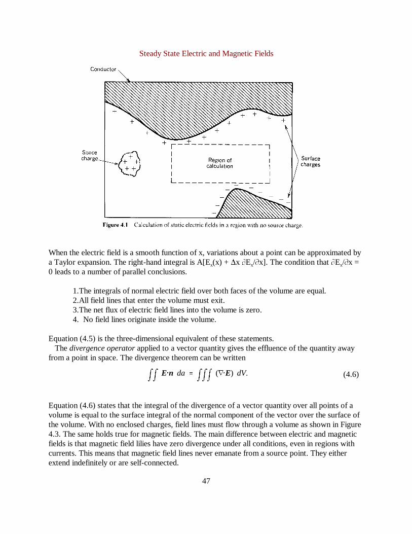
These equations resolve into two decoupled and parallel sets for electric fields [Eqs. (4.1) and(4.2)] and magnetic fields [Eqs. (4.3) and (4.4)]. Equations (4.1)-(4.4) hold in regions such as thatshown in Figure 4.1. The charges or currents that produce the fields are external to the volume ofinterest. In electrostatic calculations, the most common calculation involves charge distributed onthe surfaces of conductors at the boundaries of a vacuum region.

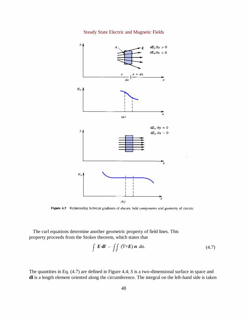
Equations (4.1)-(4.4) have straightforward physical interpretations. Similar conclusions hold forboth sets, so we will concentrate on electric fields. The form for the divergence equation [Eq.(4.1)] in Cartesian coordinates is

An example is illustrated in Figure 4.2. The electric field is a function of x and y. The meaning ofthe divergence equation can be demonstrated by calculating the integral of the normal electricfield over the surface of a volume with cross-sectional area A and thickness∆x. The integral overthe left-hand side is AEx(x). If the electric field is visualized in terms of vector field lines, theintegral is the flux of lines into the volume through the left-hand face. The electric field line fluxout of the volume through the right-hand face is AEx(x + ∆x).


47

�� E�n da � �� (��E) dV. (4.6)

When the electric field is a smooth function of x, variations about a point can be approximated bya Taylor expansion. The right-hand integral is A[Ex(x) + ∆x �Ex/�x]. The condition that�Ex/�x =0 leads to a number of parallel conclusions.

1.The integrals of normal electric field over both faces of the volume are equal.2.All field lines that enter the volume must exit.3.The net flux of electric field lines into the volume is zero.4. No field lines originate inside the volume.

Equation (4.5) is the three-dimensional equivalent of these statements.Thedivergence operatorapplied to a vector quantity gives the effluence of the quantity away

from a point in space. The divergence theorem can be written

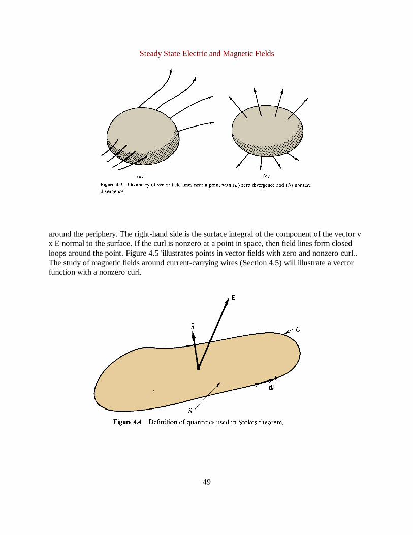
Equation (4.6) states that the integral of the divergence of a vector quantity over all points of avolume is equal to the surface integral of the normal component of the vector over the surface ofthe volume. With no enclosed charges, field lines must flow through a volume as shown in Figure4.3. The same holds true for magnetic fields. The main difference between electric and magneticfields is that magnetic field lilies have zero divergence under all conditions, even in regions withcurrents. This means that magnetic field lines never emanate from a source point. They eitherextend indefinitely or are self-connected.


48

� E�dl � �� (�×E)�n da. (4.7)

The curl equations determine another geometric property of field lines. Thisproperty proceeds from the Stokes theorem, which states that

The quantities in Eq. (4.7) are defined in Figure 4.4;S is a two-dimensional surface in space anddl is a length element oriented along the circumference. The integral on the left-hand side is taken


49

around the periphery. The right-hand side is the surface integral of the component of the vector vx E normal to the surface. If the curl is nonzero at a point in space, then field lines form closedloops around the point. Figure 4.5 'illustrates points in vector fields with zero and nonzero curl..The study of magnetic fields around current-carrying wires (Section 4.5) will illustrate a vectorfunction with a nonzero curl.


50

�×E �

ux uy uz

�/�x �/�y �/�z

Ex Ey Ez

. (4.8)

�× � ux

�Ez

�y�

�Ey

�z� uy

�Ex

�z�

�Ez

�x� uz

�Ey

�x�

�Ex

�y. (4.9)

E � ��φ. (4.10)

��(�φ) � 0,

�2φ � �

2φ/�x2� �

2φ/�y2� �

2φ/�z2� 0. (4.11)

For reference, the curl operator is written in Cartesian coordinates as

The usual rule for evaluating a determinant is used. The expansion of the above expression is

The electrostatic potential functionφ can be defined when electric fields are static. The electricfield is the gradient of this function,

Substituting forE in Eq. (4.1) gives

or

The operator symbolized by�2 in Eq. (4.11) is called the Laplacian operator. Equation (4.11) istheLaplace equation. It determines the variation ofφ (and henceE) in regions with no charge.


51

The curl equation is automatically satisfied through the vector identity�×(�φ)= 0.The main reason for using the Laplace equation rather than solving for electric fields directly is

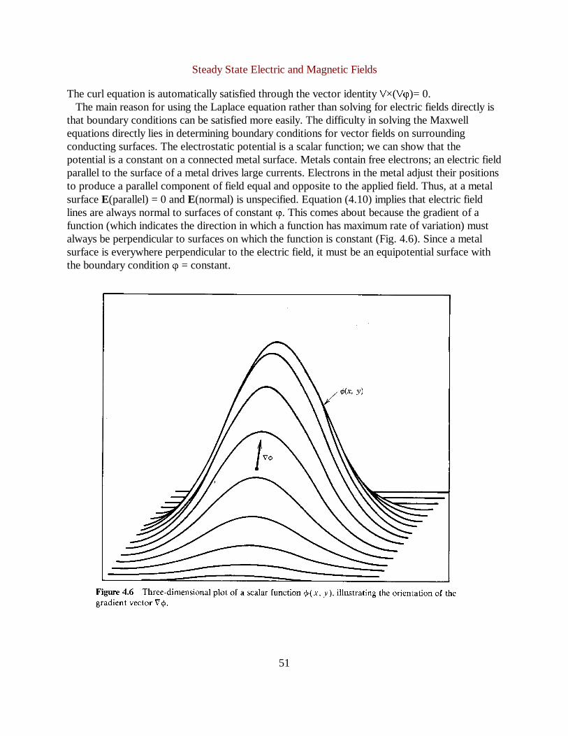
that boundary conditions can be satisfied more easily. The difficulty in solving the Maxwellequations directly lies in determining boundary conditions for vector fields on surroundingconducting surfaces. The electrostatic potential is a scalar function; we can show that thepotential is a constant on a connected metal surface. Metals contain free electrons; an electric fieldparallel to the surface of a metal drives large currents. Electrons in the metal adjust their positionsto produce a parallel component of field equal and opposite to the applied field. Thus, at a metalsurfaceE(parallel) = 0 andE(normal) is unspecified. Equation (4.10) implies that electric fieldlines are always normal to surfaces of constantφ. This comes about because the gradient of afunction (which indicates the direction in which a function has maximum rate of variation) mustalways be perpendicular to surfaces on which the function is constant (Fig. 4.6). Since a metalsurface is everywhere perpendicular to the electric field, it must be an equipotential surface withthe boundary conditionφ = constant.


52

In summary, electric field lines have the following properties in source-freeregions:

(a) Field lines are continuous. All lines that enter a volume eventually exit.(b)Field lines do not kink, curl, or cross themselves.(c)Field lines do not cross each other, since this would result in a point of infinite flux.(d)Field lines are normal to surfaces of constant electrostatic potential.(e) Electric fields are perpendicular to metal surfaces.

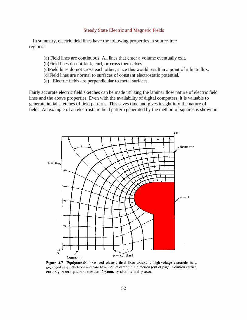
Fairly accurate electric field sketches can be made utilizing the laminar flow nature of electric fieldlines and the above properties. Even with the availability of digital computers, it is valuable togenerate initial sketches of field patterns. This saves time and gives insight into the nature offields. An example of an electrostatic field pattern generated by the method of squares is shown in


53

�2Um � 0. (4.12)

�φ(x�∆/2)/�x � [Φ(i�1,j,k)�Φ(i,j,k)]/∆. (4.13)

�

�x�φ(x)�x

�1∆

�φ(x�∆/2)�x

�

�φ(x�∆/2)�x

Figure 4.7. In this method, a number of equipotential lines between metal surfaces are sketched.Electric field lines normal to the equipotential lines and electrodes are added. Since the density offield lines is proportional to the distance between equipotentials, a valid final solution results whenthe elements between equipotential and field lines approach as close as possible to squares. Theprocess is iterative and requires only some drawing ability and an eraser.

It is also possible to define formally a magnetic potential Um such that

The function Um should not be confused with the vector potential. Methods used for electric fieldproblems in source-free regions can also be applied to determine magnetic fields. We will deferuse of Eq. (4.12) to Chapter 5. An understanding of magnetic materials is necessary to determineboundary conditions for Um.

4.2 NUMERICAL SOLUTIONS TO THE LAPLACE EQUATION

The Laplace equation determines electrostatic potential as a function of position. Resultingelectric fields can then be used to calculate particle orbits. Electrostatic problems may involvecomplex geometries with surfaces at many different potentials. In this case, numerical methods ofanalysis are essential.

Digital computers handle discrete quantities, so the Laplace equation must be converted from acontinuous differential equation to a finite difference formulation. As shown in Figure 4.8, thequantityΦ(i, j, k) is defined at discrete points in space. These points constitute athree-dimensional mesh. For simplicity, the mesh spacing∆ between points in the three Cartesiandirections is assumed uniform. The quantityΦ has the property that it equalsφ(x, y, z) at themesh points. Ifφ is a smoothly varying function, then a linear interpolation ofΦ gives a goodapproximation forφ at any point in space. In summary,Φ is a mathematical construct used toestimate the physical quantity,φ.

The Laplace equation forφ implies an algebraic difference equation forΦ. The spatial positionof a mesh point is denoted by (i, j, k), with x = i∆, y = j∆, and z = k∆. The x derivative ofφ tothe right of the point (x, y, z) is approximated by

A similar expression holds for the derivative at x -∆/2. The second derivative is the difference ofderivatives divided by∆, or


54

�2φ

�x2�

Φ(i�1,j,k) � 2Φ(i,j,k) � Φ(i�1,j,k)]

∆2. (4.14)

Φ(i,j,k) � 1/6 [Φ(i�1,j,k) � Φ(i�1,j,k) � Φ(i,j�1,k)

� Φ(i,j�1,k) � Φ(i,j,k�1) � Φ(i,j,k�1)].(4.15)

Combining expressions,

Similar expressions can be found for the�2φ/�y2 and�2φ/�z2 terms. Setting�2φ1 = 0 implies

In summary, (1)Φ(i, j, k) is a discrete function defined as mesh points, (2) the interpolation ofΦ(i, j, k) approximatesφ(x, y, z), and (3) ifφ(x, y, z) satisfies the Laplace equation, thenΦ(i, j, k)is determined by Eq. (4.15).

According to Eq. (4.15), individual values ofΦ(i, j, k) are the average of their six neighboring


55

R(i,j) � ¼[Φ(i�1,j) � Φ(i�1,j) � Φ(i,j�1) � Φ(i,j�1)] � Φ(i,j) (4.16)

Φ(i,j)n�1 � Φ(i,j)n � ωR(i,j)n. (4.17)

points. Solving the Laplace equation is an averaging process; the solution gives the smoothestflow of field lines. The net length of all field lines is minimized consistent with the boundaryconditions. Therefore, the solution represents the state with minimum field energy (Section 5.6).

There are many numerical methods to solve the finite difference form for the Laplace equation.We will concentrate on themethod of successive ouerrelaxation. Although it is not the fastestmethod of solution, it has the closest relationship to the physical content of the Laplace equation.To illustrate the method, the problem will be formulated on a two-dimensional, square mesh.Successive overrelaxation is an iterative approach. A trial solution is corrected until it is close to avalid solution. Correction consists of sweeping through all values of an intermediate solution tocalculateresiduals, defined by

If R(i, j) is zero at all points, thenΦ(i, j) is the desired solution. An intermediate result can beimproved by adding a correction factor proportional to R(i, j),

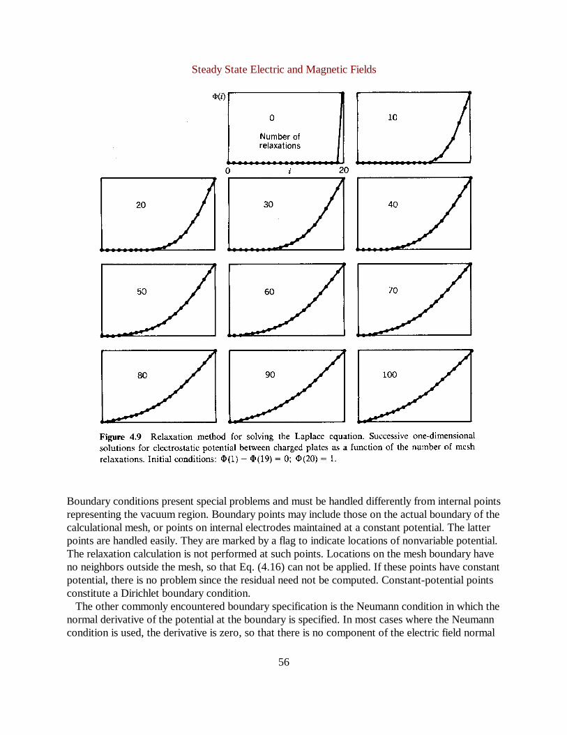
The valueω = 1 is the obvious choice, but in practice values ofω between 1 and 2 produce afaster convergence (hence the term overrelaxation). The succession of approximations resemblesa time-dependent solution for a system with damping, relaxing to its lowest energy state. Theelastic sheet analog (described in Section 4.3) is a good example of this interpretation. Figure 4.9shows intermediate solutions for a one-dimensional mesh with 20 points and withω = 1.00.Information on the boundary with elevated potential propagates through the mesh.

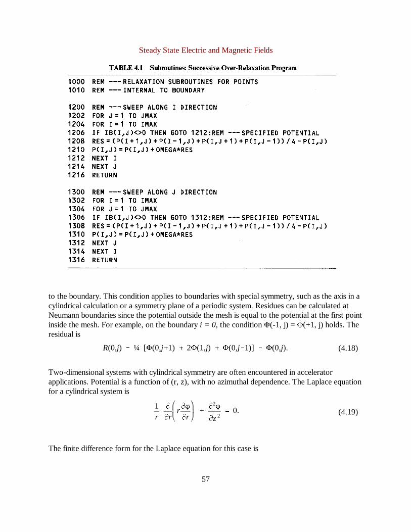
The method of successive overrelaxation is quite slow for large numbers of points. The numberof calculations on ann x nmesh is proportional ton2. Furthermore, the number of iterationsnecessary to propagate errors out of the mesh is proportional to n. The calculation time increasesas n3 . A BASIC algorithm to relax internal points in a 40 x 48 point array is listed in Table 4.1.Corrections are made continuously during the sweep. Sweeps are first carried out along thexdirection and then along they direction to allow propagation of errors in both directions. Theelectrostatic field distribution in Figure 4.10 was calculated by a relaxation program.

Advanced methods for solving the Laplace equation generally use more efficient algorithmsbased on Fourier transforms. Most available codes to solve electrostatic problems utilize a morecomplex mesh. The mesh may have a rectangular or even triangular divisions to allow a closematch to curved boundary surfaces.


56

Boundary conditions present special problems and must be handled differently from internal pointsrepresenting the vacuum region. Boundary points may include those on the actual boundary of thecalculational mesh, or points on internal electrodes maintained at a constant potential. The latterpoints are handled easily. They are marked by a flag to indicate locations of nonvariable potential.The relaxation calculation is not performed at such points. Locations on the mesh boundary haveno neighbors outside the mesh, so that Eq. (4.16) can not be applied. If these points have constantpotential, there is no problem since the residual need not be computed. Constant-potential pointsconstitute a Dirichlet boundary condition.

The other commonly encountered boundary specification is the Neumann condition in which thenormal derivative of the potential at the boundary is specified. In most cases where the Neumanncondition is used, the derivative is zero, so that there is no component of the electric field normal


57

R(0,j) � ¼ [Φ(0,j�1) � 2Φ(1,j) � Φ(0,j�1)] � Φ(0,j). (4.18)

1r

�

�rr�φ

�r�

�2φ

�z2� 0. (4.19)

to the boundary. This condition applies to boundaries with special symmetry, such as the axis in acylindrical calculation or a symmetry plane of a periodic system. Residues can be calculated atNeumann boundaries since the potential outside the mesh is equal to the potential at the first pointinside the mesh. For example, on the boundaryi = 0 , the conditionΦ(-1, j) = Φ(+1, j) holds. Theresidual is

Two-dimensional systems with cylindrical symmetry are often encountered in acceleratorapplications. Potential is a function of (r, z), with no azimuthal dependence. The Laplace equationfor a cylindrical system is

The finite difference form for the Laplace equation for this case is


58

Φ(i,j) �14

(i�½)Φ(i�1,j)i

�

(i�½)Φ(i�1,j)i

� Φ(i,j�1) � Φ(i,j�1) . (4.20)

where r = i∆ and z = j∆.Figure 4.10 shows results for a relaxation calculation of an electrostatic immersion lens. It

consists of two cylinders at different potentials separated by a gap. Points of constant potentialand Neumann boundary conditions are indicated. Also shown is the finite differenceapproximation for the potential variation along the axis, 0(0, z). This data can be used todetermine the focal properties of the lens (Chapter 6).

4.3 ANALOG METHODS TO SOLVE THE LAPLACE EQUATION

Analog methods were used extensively to solve electrostatic field problems before the advent ofdigital computers. We will consider two analog techniques that clarify the nature of the Laplaceequation. The approach relies on finding a physical system that obeys the Laplace equation butthat allows easy measurements of a characteristic quantity (the analog of the potential).

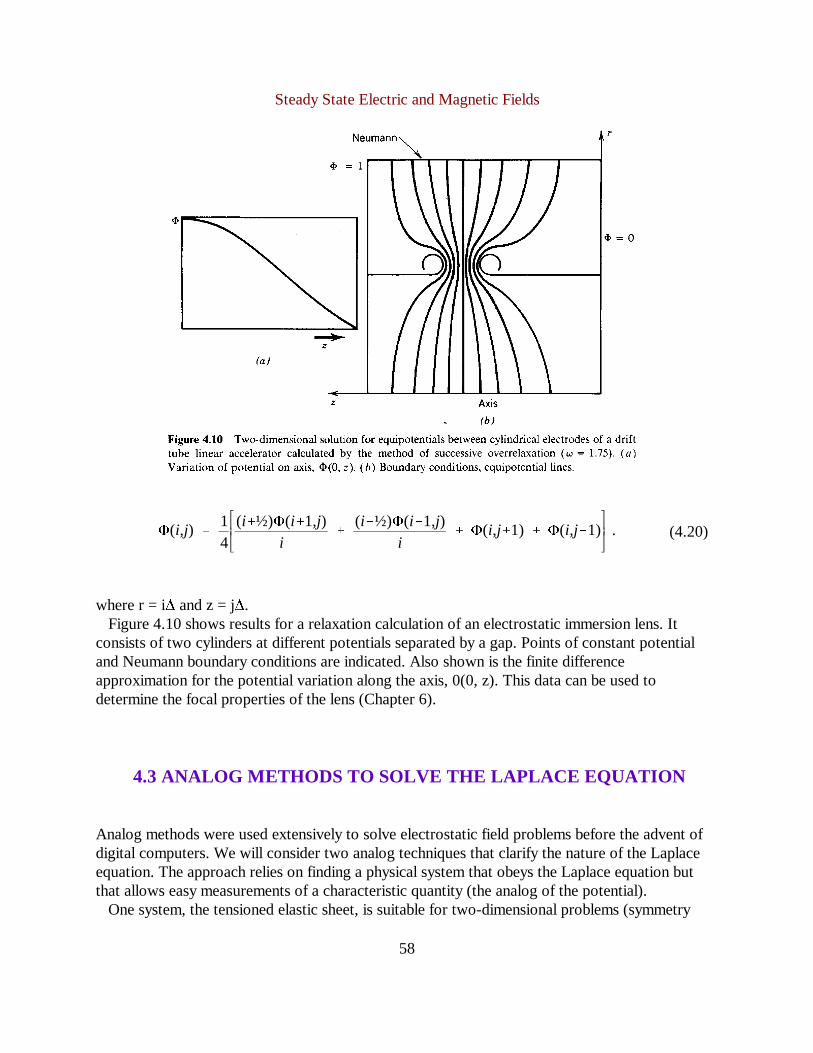
One system, the tensioned elastic sheet, is suitable for two-dimensional problems (symmetry


59

F[(i�½)∆] � T [H(i∆,j∆)�H([i�1]∆,j∆)]/∆,

F[(i�½)∆] � T [H([i�1]∆,j∆)�H(i∆,j∆)]/∆.

F[(i�½)∆] � �F[(i�½)∆],

F[(j�½)∆] � �F[(j�½)∆].

�2H(x,y)/�x2

� �2H(x,y)/�y2

� 0.

along the z axis). As shown in Figure 4.11, a latex sheet is stretched with uniform tension on aframe. If the sheet is displaced vertically a distanceH(x, y), there will be vertical restoring forces.In equilibrium, there is vertical force balance ateach point. The equation of force balance can bedetermined from the finite difference approximation defined in Figure 4.11. In terms of the surfacetension, the forces to the left and right of the point (i∆, j∆) are

Similar expressions can be determined for they direction. The height of the point (i∆, j∆) isconstant in time; therefore,

and

Substituting for the forces shows that the height of a point on a square mesh is the average of itsfour nearest neighbors. Thus, inverting the arguments of Section 4.2,H(x, y) is described by thetwo-dimensional Laplace equation


60

E � ρ j

Height is the analog of potential. To make an elastic potential solution, parts are cut to theshape of the electrodes. They are fastened to the frame to displace the elastic sheet up or down adistance proportional to the electrode potential. These pieces determine equipotential surfaces.The frame is theground plane.

An interesting feature of the elastic sheet analog is that it can also be used to determine orbits ofcharged particles in applied electrostatic fields. Neglecting rotation, the total energy of a ballbearing on the elastic sheet isE = T + mgh(x, y), where g is the gravitational constant. Thetransverse forces acting on a ball bearing on the elastic sheet are Fx = �H/�x and Fy = �H/�y.Thus, ball bearings on the elastic sheet follow the same orbits as charged particles in theanalogous electrostatic potential, although over a considerably longer time scale.

Figure 4.12 is a photograph of a model that demonstrates the potentials in a planar electronextraction gap with a coarse grid anode made of parallel wires. The source of the facet lens effectassociated with extraction grids (Section 6.5) is apparent.

A second analog technique, the electrolytic tank, permits accurate measurements of potentialdistributions. The method is based on the flow of current in a liquid medium of constant-volumeresistivity,ρ (measured in units of ohm-meters). A dilute solution of copper sulfate in water is acommon medium. A model of the electrode structure is constructed to scale from copper sheetand immersed in the solution. Alternating current voltages with magnitude proportional to thosein the actual system are applied to the electrodes.

According to the definition of volume resistivity, the current density is proportional to theelectric field

Figure 4.12 Elastic sheet analog for electrostatic potential near an extraction grid. Elevatedsection represents a high-voltage electrode surrounded by a grounded enclosure. Note thedistortion of the potential near the grid wires that results in focusing of extracted particles.(Photograph and model by the author. Latex courtesy of the Hygenic Corporation.)


61

j � ��φ/ρ. (4.21)

��j � 0. (4.22)

or

The steady-state condition that charge at any point in the liquid is a constant implies that allcurrent that flows into a volume element must flow out. This condition can be written

Combining Eq. (4.21) with (4.22), we find that potential in the electrolytic solution obeys theLaplace equation.

In contrast to the potential in the real system, the potential in the electrolytic analog ismaintained by a real current flow. Thus, energy is available for electrical measurements. Ahigh-impedance probe can be inserted into the solution without seriously perturbing the fields.Although the electrolytic method could be applied to three-dimensional problems, in practice it isusually limited to two-dimensional simulations because oflimitations on insertion of a probe. Atypical setup is shown in Figure 4.13. Following the arguments given above, it is easy to showthat a tipped tank can be used to solve for potentials in cylindrically symmetric systems.

4.4 ELECTROSTATIC QUADRUPOLE FIELD

Although numerical calculations are often necessary to determine electric and magnetic fields inaccelerators, analytic calculations have advantages when they are tractable. Analytic solutionsshow general features and scaling relationships. The field expressions can be substituted intoequations of motion to yield particle orbit expressions in closed form. Electrostatic solutions for awide variety of electrode geometries have been derived. In this section. we will examine thequadrupole field, a field configuration used in all high-energy transport systems. We willconcentrate on the electrostatic quadrupole; the magnetic equivalent will be discussed in Chapter


62

Ex � �kx � Eox/a, (4.23)

Ey � �ky � �Eoy/a. (4.24)

�φ/�x � �Eox/a, �φ/�y � �Eoy/a,

φ � �Eox2/2a � f(y) � C, φ � �Eoy

2/2a � g(x) � C �.

φ(x,y) � (Eo/2a) (y2� x2). (4.25)

φ(x,y)Eoa/2

�

ya

2

�

xa

2

. (4.26)

5.The most effective procedure to determine electrodes to generate quadrupole fields is to work

in reverse, starting with the desired electric field distribution and calculating the associatedpotential function. The equipotential lines determine a set of electrode surfaces and potentials thatgenerate the field. We assume the following two-dimensional fields:

It is straightforward to verify that both the divergence and curl ofE are zero. The fields of Eqs.(4.23) and (4.24) represent a valid solution to the Maxwell equations in a vacuum region. Theelectric fields are zero at the axis and increase (or decrease) linearly with distance from the axis.The potential is related to the electric field by

Integrating the partial differential equations

Takingφ(0, 0) = 0, both expressions are satisfied if

This can be rewritten in a more convenient, dimensionless form:

Equipotential surfaces are hyperbolas in all four quadrants. There is an infinite set of electrodesthat will generate the fields of Eqs. (4.23) and (4.24). The usual choice is symmetric electrodes onthe equipotential linesφo = ±E oa/2. Electrodes, field lines, and equipotential surfaces are plottedin Figure 4.14. The quantitya is the minimum distance from the axis to the electrode, and Eo isthe electric field on the electrode surface at the position closest to the origin. The equipotentials inFigure 4.14 extend to infinity. In practice, focusing fields are needed only near the axis. Thesefields are not greatly affected by terminating the electrodes at distances a few times a fromthe axis.


63


64

��E � (ρ1 � ρ2 � ρ3)/εo. (4.27)

E � E1(applied) � E2(dielectric) � E3(spacecharge). (4.28)

4.5 STATIC ELECTRIC FIELDS WITH SPACE CHARGE

Space chargeis charge density present in the region in which an electric field is to be calculated.Clearly, space charge is not included in the Laplace equation, which describes potential arisingfrom charges on external electrodes. In accelerator applications, space charge is identified withthe charge of the beam; it must be included in calculations of fields internal to the beam. Althoughwe will not deal with beam self-fields in this book, it is useful to perform at least one space chargecalculation. It gives insight into the organization of various types of charge to derive electrostaticsolutions. Furthermore, we will derive a useful formula to estimate when beam charge can beneglected.

Charge density can be conveniently divided into three groups: (1) applied, (2) dielectric, and (3)space charge. Equation 3.13 can be rewritten

The quantityρ1 is the charge induced on the surfaces of conducting electrodes by the applicationof voltages. The second charge density represents charges indielectric materials. Electrons indielectric materials cannot move freely. They are bound to a positive charge and can be displacedonly a small distance. The dielectric charge density can influence fields in and near the material.Electrostatic calculations with the inclusion ofρ2 are discussed in Chapter 5. The final chargedensity,ρ3, represents space charge, or free charge in the region of the calculation. This usuallyincludes the charge density of the beam. Other particles may contribute toρ3, such as low-energyelectrons in a neutralized ion beam.

Electric fields have the property of superposition. Given fields corresponding to two or morecharge distributions, then the total electric field is the vector sum of the individual fields if thecharge distributions do not perturb one another. For instance, we could calculate electric fieldsindividually for each of the charge components,El, E2, andE3. The total field is

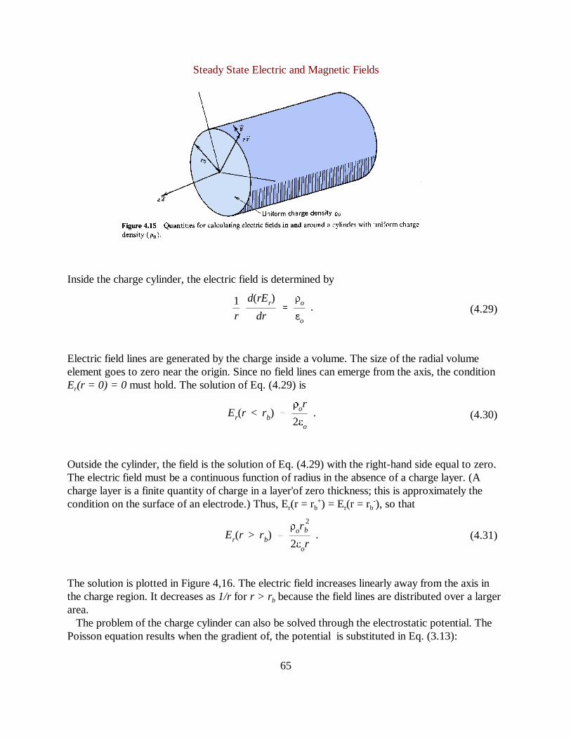
Only the third component occurs in the example of Figure 4.15. The cylinder with uniform chargedensity is a commonly encountered approximation for beam space charge. The charge density isconstant,ρo, from r = 0 to r = rb. There is no variation in the axial (z) or azimuthal (θ) directionsso that�/�z = �/�θ = 0. The divergence equation (3.13) implies that there is only a radialcomponent of electric field. Because all field lines radiate straight outward (or inward forρo < 0),there can be no curl, and Eq. (3.11) is automatically satisfied.


65

1r

d(rEr)

dr�

ρo

εo

. (4.29)

Er(r < rb) �ρor

2εo

. (4.30)

Er(r > rb) �ρor

2b

2εor. (4.31)

Inside the charge cylinder, the electric field is determined by

Electric field lines are generated by the charge inside a volume. The size of the radial volumeelement goes to zero near the origin. Since no field lines can emerge from the axis, the conditionEr(r = 0) = 0 must hold. The solution of Eq. (4.29) is

Outside the cylinder, the field is the solution of Eq. (4.29) with the right-hand side equal to zero.The electric field must be a continuous function of radius in the absence of a charge layer. (Acharge layer is a finite quantity of charge in a layer'of zero thickness; this is approximately thecondition on the surface of an electrode.) Thus, Er(r = rb

+) = Er(r = rb-), so that

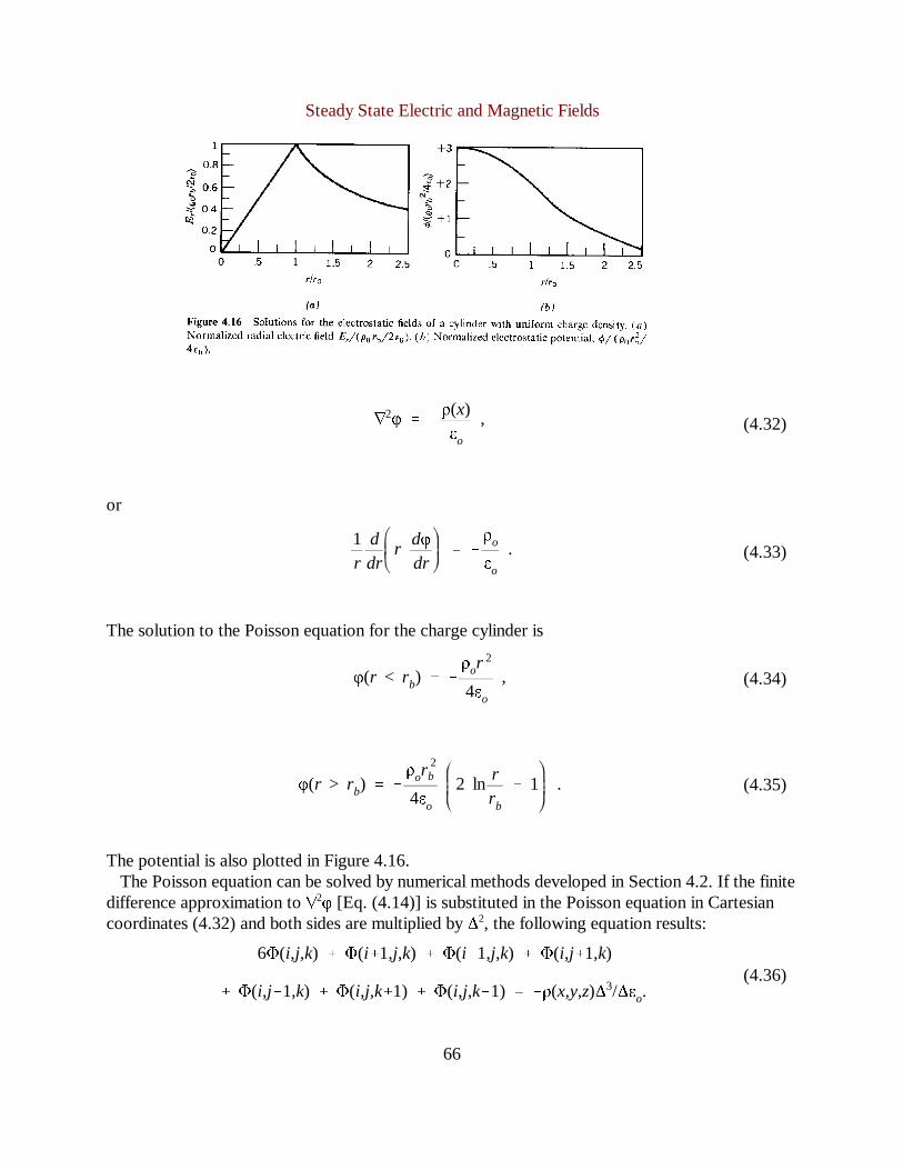
The solution is plotted in Figure 4,16. The electric field increases linearly away from the axis inthe charge region. It decreases as1/r for r > r b because the field lines are distributed over a largerarea.

The problem of the charge cylinder can also be solved through the electrostatic potential. ThePoisson equation results when the gradient of, the potential is substituted in Eq. (3.13):


66

�2φ � �

ρ(x)εo

, (4.32)

1r

ddr

rdφdr

� �

ρo

εo

. (4.33)

φ(r < rb) � �

ρor2

4εo

, (4.34)

φ(r > rb) � �

ρor2b

4εo

2 lnrrb

� 1 . (4.35)

�6Φ(i,j,k) � Φ(i�1,j,k) � Φ(i�1,j,k) � Φ(i,j�1,k)

� Φ(i,j�1,k) � Φ(i,j,k�1) � Φ(i,j,k�1) � �ρ(x,y,z)∆3/∆εo.(4.36)

or

The solution to the Poisson equation for the charge cylinder is

The potential is also plotted in Figure 4.16.The Poisson equation can be solved by numerical methods developed in Section 4.2. If the finite

difference approximation to�2φ [Eq. (4.14)] is substituted in the Poisson equation in Cartesiancoordinates (4.32) and both sides are multiplied by∆2, the following equation results:


67

Φ(i,j,k) � 1/6 [Φ(i�1,j,k) � Φ(i�1,j,k) � Φ(i,j�1,k)

� Φ(i,j�1,k) � Φ(i,j,k�1) � Φ(i,j,k�1)] � Q(i,j,k)/6εo.(4.37)

R(i,j,) � 1/4 [Φ(i�1,j) � Φ(i�1,j) � Φ(i,j�1) � Φ(i,j�1)]

� Φ(i,j) � Q(i,j)/4εo .(4.38)

� B�dl � µo �� jzdA � µoI. (4.39)

Bθ� µoI/2πr. (4.40)

The factorρ∆3 is approximately the total charge in a volume∆3 surrounding the mesh point(i, j,k)when (1) the charge density is a smooth function of position and (2) the distance∆ is smallcompared to the scale length for variations inρ. Equation (4.36) can be converted to a finitedifference equation by defining Q(i, j, k) =ρ(x, y, z)∆3. Equation (4.36) becomes

Equation (4.37) states that the potential at a point is the average of 'its nearest neighbors elevated(or lowered) by a term proportional to the space charge surrounding the point.

The method of successive relaxation can easily be modified to treat problems with space charge.In this case, the residual [Eq. (4.16)] for a two-dimensional problem is

4.6 MAGNETIC FIELDS IN SIMPLE GEOMETRIES

This section illustrates some methods to find static magnetic fields by direct use of the Maxwellequations [(4.3) and (4.4)]. The fields are produced by current-carrying wires. Two simple, butoften encountered, geometries are included: the field outside a long straight wire and the fieldinside of solenoidal winding of infinite extent.

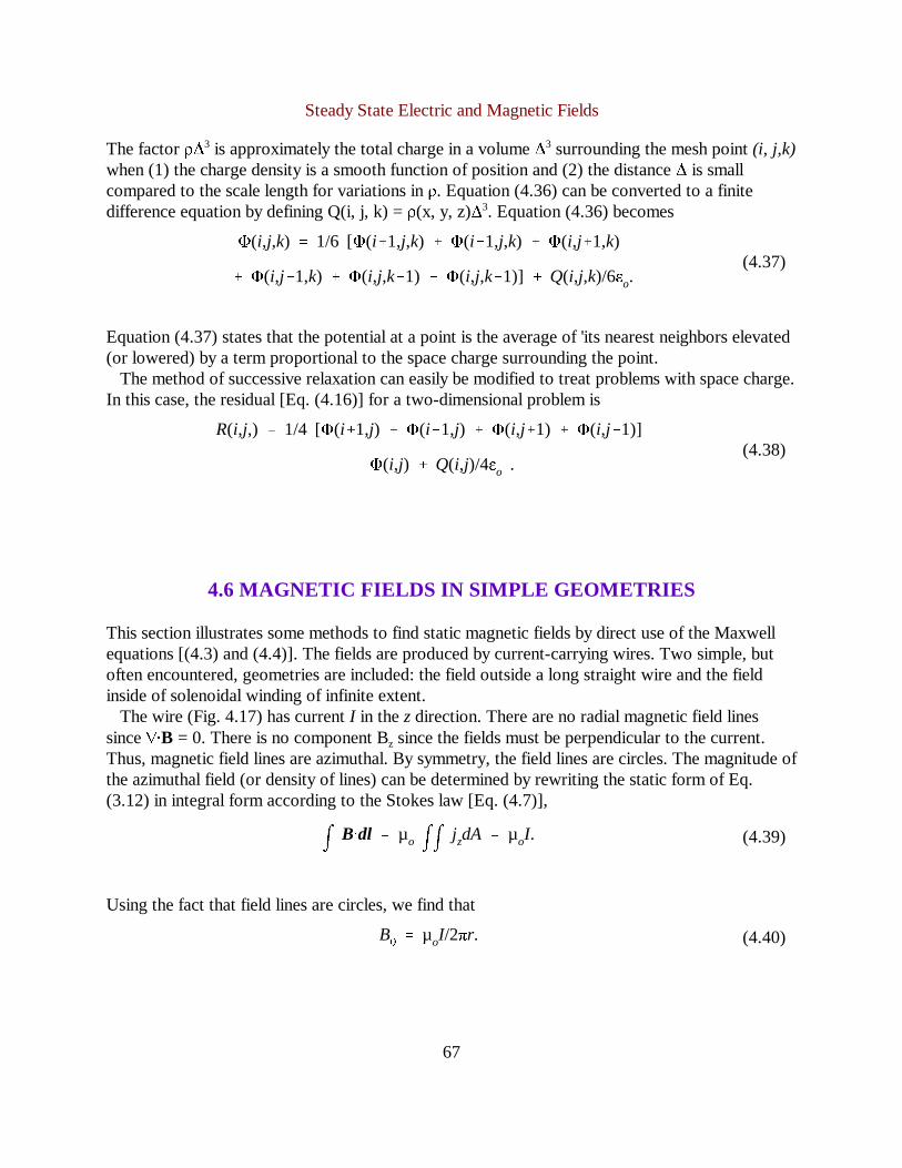
The wire (Fig. 4.17) has currentI in thez direction. There are no radial magnetic field linessince��B = 0. There is no component Bz since the fields must be perpendicular to the current.Thus, magnetic field lines are azimuthal. By symmetry, the field lines are circles. The magnitude ofthe azimuthal field (or density of lines) can be determined by rewriting the static form of Eq.(3.12) in integral form according to the Stokes law [Eq. (4.7)],

Using the fact that field lines are circles, we find that


68

1r

�(rBr)

�r�

�Bz

�z� 0,

�Br

�z�

�Bz

�r� 0. (4.41)

Bo � µo J � µo (N/L) I. (4.42)

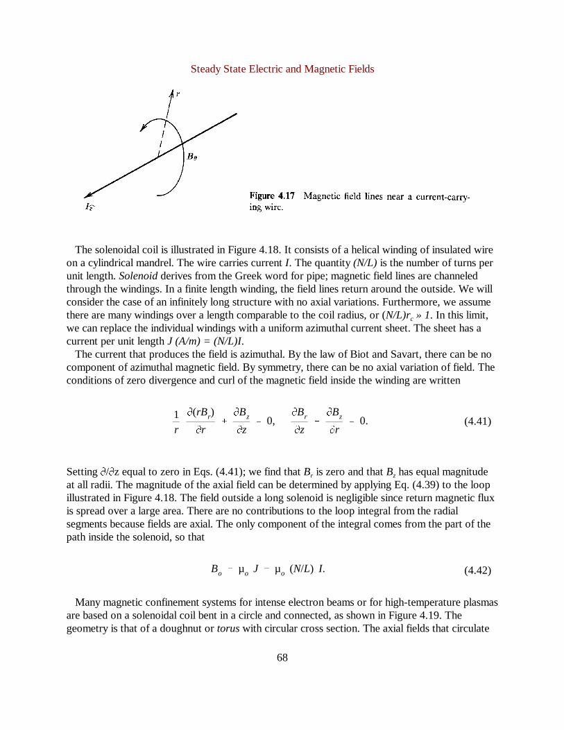
The solenoidal coil is illustrated in Figure 4.18. It consists of a helical winding of insulated wireon a cylindrical mandrel. The wire carries currentI. The quantity(N/L) is the number of turns perunit length.Solenoidderives from the Greek word for pipe; magnetic field lines are channeledthrough the windings. In a finite length winding, the field lines return around the outside. We willconsider the case of an infinitely long structure with no axial variations. Furthermore, we assumethere are many windings over a length comparable to the coil radius, or (N/L)rc » 1. In this limit,we can replace the individual windings with a uniform azimuthal current sheet. The sheet has acurrent per unit lengthJ (A/m) = (N/L)I.

The current that produces the field is azimuthal. By the law of Biot and Savart, there can be nocomponent of azimuthal magnetic field. By symmetry, there can be no axial variation of field. Theconditions of zero divergence and curl of the magnetic field inside the winding are written

Setting�/�z equal to zero in Eqs. (4.41); we find thatBr is zero and thatBz has equal magnitudeat all radii. The magnitude of the axial field can be determined by applying Eq. (4.39) to the loopillustrated in Figure 4.18. The field outside a long solenoid is negligible since return magnetic fluxis spread over a large area. There are no contributions to the loop integral from the radialsegments because fields are axial. The only component of the integral comes from the part of thepath inside the solenoid, so that

Many magnetic confinement systems for intense electron beams or for high-temperature plasmasare based on a solenoidal coil bent in a circle and connected, as shown in Figure 4.19. Thegeometry is that of a doughnut ortoruswith circular cross section. The axial fields that circulate


69

around the torus are calledtoroidal field lines. Field lines are continuous and self-connected. Allfield lines are contained within the winding. The toroidal field magnitude inside the winding is notuniform. Modification of the loop construction of Figure 4.19 shows that the field varies as theinverse of the major radius. Toroidal field variation is small when the minor radius (the radius ofthe solenoidal windings) is much less than the major radius.


70

Bx � �Az/�y, By � ��Az/�x. (4.43)

dAz � 0 � (�Az/�x) dx � (�Az/�y) dy. (4.44)

4.7 MAGNETIC POTENTIALS

The magnetic potential and the vector potential aid in the calculation of magnetic fields. In thissection, we will consider how these functions are related and investigate the physical meaning ofthe vector potential in a two-dimensional geometry. The vector potential will be used to derivethe magnetic field for a circular current loop. Assemblies of loop currents are used to generatemagnetic fields in many particle beam transport devices.

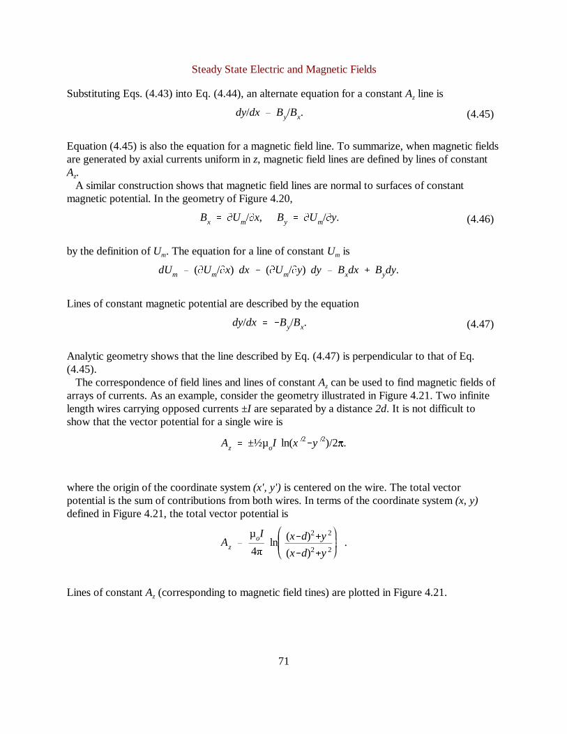
In certain geometries, magnetic field lines and the vector potential are closely related. Figure4.20 illustrates lines of constant vector potential in an axially uniform system in which fields aregenerated by currents in thez direction. Equation (3.24) implies that the vector potential has onlyan axial component,Az. Equation (3.23) implies that

Figure 4.20 shows a surface of constantAz in the geometry considered. This line is defined by


71

dy/dx � By/Bx. (4.45)

Bx � �Um/�x, By � �Um/�y. (4.46)

dUm � (�Um/�x) dx � (�Um/�y) dy � Bxdx � Bydy.

dy/dx � �By/Bx. (4.47)

Az � ±½µoI ln(x �2�y �2)/2π.

Az �µoI

4πln

(x�d)2�y2

(x�d)2�y2

.

Substituting Eqs. (4.43) into Eq. (4.44), an alternate equation for a constantAz line is

Equation (4.45) is also the equation for a magnetic field line. To summarize, when magnetic fieldsare generated by axial currents uniform inz, magnetic field lines are defined by lines of constantAz.

A similar construction shows that magnetic field lines are normal to surfaces of constantmagnetic potential. In the geometry of Figure 4.20,

by the definition ofUm. The equation for a line of constantUm is

Lines of constant magnetic potential are described by the equation

Analytic geometry shows that the line described by Eq. (4.47) is perpendicular to that of Eq.(4.45).

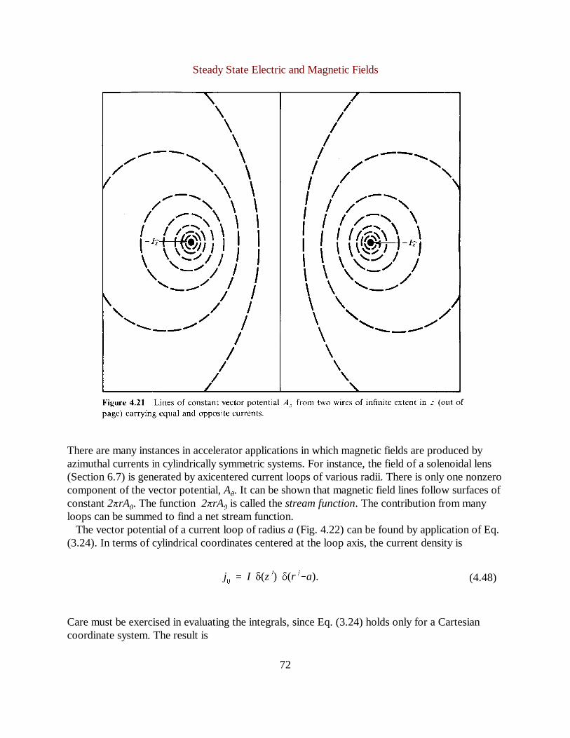
The correspondence of field lines and lines of constantAz can be used to find magnetic fields ofarrays of currents. As an example, consider the geometry illustrated in Figure 4.21. Two infinitelength wires carrying opposed currents±I are separated by a distance2d. It is not difficult toshow that the vector potential for a single wire is

where the origin of the coordinate system(x', y') is centered on the wire. The total vectorpotential is the sum of contributions from both wires. In terms of the coordinate system(x, y)defined in Figure 4.21, the total vector potential is

Lines of constantAz (corresponding to magnetic field tines) are plotted in Figure 4.21.


72

jθ� I δ(z�) δ(r �

�a). (4.48)

There are many instances in accelerator applications in which magnetic fields are produced byazimuthal currents in cylindrically symmetric systems. For instance, the field of a solenoidal lens(Section 6.7) is generated by axicentered current loops of various radii. There is only one nonzerocomponent of the vector potential,A

θ. It can be shown that magnetic field lines follow surfaces of

constant2πrAθ. The function 2πrA

θis called thestream function. The contribution from many

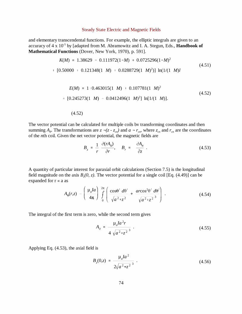
loops can be summed to find a net stream function.The vector potential of a current loop of radiusa (Fig. 4.22) can be found by application of Eq.

(3.24). In terms of cylindrical coordinates centered at the loop axis, the current density is

Care must be exercised in evaluating the integrals, since Eq. (3.24) holds only for a Cartesiancoordinate system. The result is


73

Aθ�

µoIa

4π �

2π

0

cosθ�dθ�

(a 2� r 2

� z2� 2ar cosθ�)½

. (4.49)

M � 4ar/(a 2� r 2

� z2� 2ar),

Aθ�

µoIa

π (a 2� r 2

� z2� 2ar)½

(2�M) K(M) � 2 E(M)M

. (4.50)

Defining the quantity

Eq. (4.49) can be written in terms of the complete elliptic integrals E(M) and K(M) as

Although the expressions in Eq. (4.50) are relatively complex, the vector potential can becalculated quickly on a computer. Evaluating the elliptic integrals directly is usually ineffectiveand time consuming. A better approach is to utilize empirical series tabulated in manymathematical handbook s. These series give an accurate approximation in terms of power series


74

K(M) � 1.38629� 0.111972(1�M) � 0.0725296(1�M)2

� [0.50000� 0.121348(1�M) � 0.0288729(1�M)2)] ln(1/(1�M)l(4.51)

E(M) � 1�0.463015(1�M) � 0.107781(1�M)2

� [0.245273(1�M) � 0.0412496(1�M)2] ln[1/(1�M)].(4.52)

Bz �1r

�(rAθ)

�r, Br � �

�Aθ

�z. (4.53)

Aθ(r,z) �

µoIa

4π �

2π

0

cosθ� dθ�

a 2�z2

�

arcos2θ� dθ�

a 2�z2 3

. (4.54)

Aθ�

µoIa2r

4 a 2�z2 3

. (4.55)

Bz(0,z) �µoIa

2

2 a 2�z2 3

. (4.56)

and elementary transcendental functions. For example, the elliptic integrals are given to anaccuracy of 4 x 10-5 by [adapted from M. Abramowitz and I. A. Stegun, Eds.,Handbook ofMathematical Functions (Dover, New York, 1970), p. 591].

(4.52)

The vector potential can be calculated for multiple coils bv transforming coordinates and thensummingA

θ. The transformations arez�(z - zcn) anda � rcn, wherezcn andrcn are the coordinates

of thenth coil. Given the net vector potential, the magnetic fields are

A quantity of particular interest for paraxial orbit calculations (Section 7.5) is the longitudinalfield magnitude on the axisBz(0, z). The vector potential for a single coil [Eq. (4.49)] can beexpanded for r « a as

The integral of the first term is zero, while the second term gives

Applying Eq. (4.53), the axial field is


75

Bz(0,z) � (B1�B2) � (�B1/�z � �B2/�z) z

� (�2B1/�z2� �

2B2/�z2) z2�...

Bz � µoI / (1.25)3/2 a (4.57)

We can use Eq. (4.56) to derive the geometry of the Helmholtz coil configuration. Assume thattwo loops with equal current are separated by an axial distanced. A Taylor expansion of the axialfield near the axis about the midpoint of the coils gives

The subscript1 refers to the contribution from the coil atz = - d/2, while 2 is associated with thecoil at z = + d/2. The derivatives can be determined from Eq. (4.56). The zero-order componentsfrom both coils add. The first derivatives cancel at all values of the coil spacing. At a spacing ofd= a, the second derivatives also cancel. Thus, field variations near the symmetry point are only onthe order of(z/a)3 . Two coils withd = a are called Helmholtz coils. They are used when a weakbut accurate axial field is required over a region that is small compared to the dimension of thecoil. The field magnitude for Helmholtz coils is

Steady-State Electric and Magnetic Fields

Documents

Transcript of Steady-State Electric and Magnetic Fields