Status of the Regional OSSE Status of the Regional OSSE for Space-Based LIDAR for Space-Based LIDAR

Winds – July 2002Winds – July 2002

Steve KochSteve Koch

Adrian Adrian MarroquinMarroquin

Tom SchlatterTom Schlatter

John SmartJohn Smart

Steve WeygandtSteve Weygandt

Graham Graham FeingoldFeingold

Mike HardestyMike Hardesty

Barry RyeBarry Rye

Dale BarkerDale Barker

CollaboratorsCollaborators NOAA/ETL NOAA/ETL

Lidar Simulation/ DataLidar Simulation/ Data Atmospheric propagationAtmospheric propagation

NOAA/FSLNOAA/FSL Regional Nature RunRegional Nature Run Data assimilationData assimilation AssessmentAssessment

NCARNCAR Quality assessment of model resultsQuality assessment of model results ValidationValidation

NOAA/NWS/NCEP NOAA/NWS/NCEP Global model background gridsGlobal model background grids AdviceAdvice

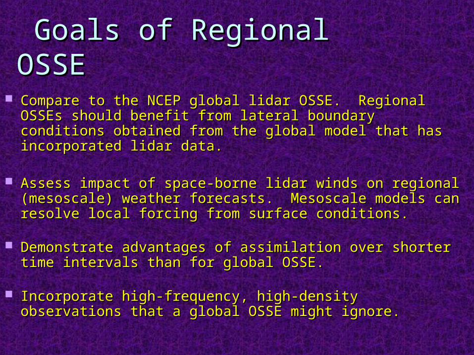
Goals of Regional OSSEGoals of Regional OSSE Compare to the NCEP global lidar OSSE. Regional OSSEs Compare to the NCEP global lidar OSSE. Regional OSSEs

should benefit from lateral boundary conditions obtained should benefit from lateral boundary conditions obtained from the global model that has incorporated lidar data.from the global model that has incorporated lidar data.

Assess impact of space-borne lidar winds on regional Assess impact of space-borne lidar winds on regional (mesoscale) weather forecasts. Mesoscale models can (mesoscale) weather forecasts. Mesoscale models can resolve local forcing from surface conditions.resolve local forcing from surface conditions.

Demonstrate advantages of assimilation over shorter Demonstrate advantages of assimilation over shorter time intervals than for global OSSE.time intervals than for global OSSE.

Incorporate high-frequency, high-density observations Incorporate high-frequency, high-density observations that a global OSSE might ignore.that a global OSSE might ignore.

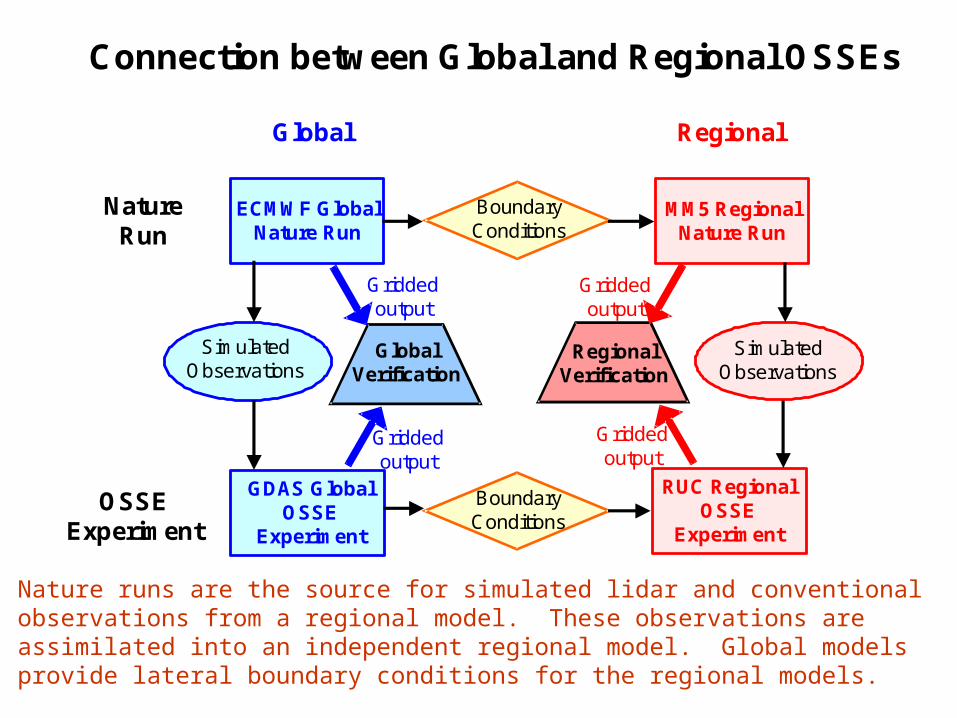
Connection between Global and Regional OSSEs

ECMWF Global Nature Run

GDAS Global OSSE

Experiment

MM5 Regional Nature Run

RUC Regional OSSE

Experiment

Global Regional

Nature Run

OSSE Experiment

Simulated Observations

Boundary Conditions

Boundary Conditions

Simulated Observations

Global Verification

Regional Verification

Griddedoutput

Griddedoutput

Griddedoutput

Griddedoutput

Nature runs are the source for simulated lidar and conventional observations from a regional model. These observations are assimilated into an independent regional model. Global models provide lateral boundary conditions for the regional models.

Regional OSSE Regional OSSE MethodologyMethodology

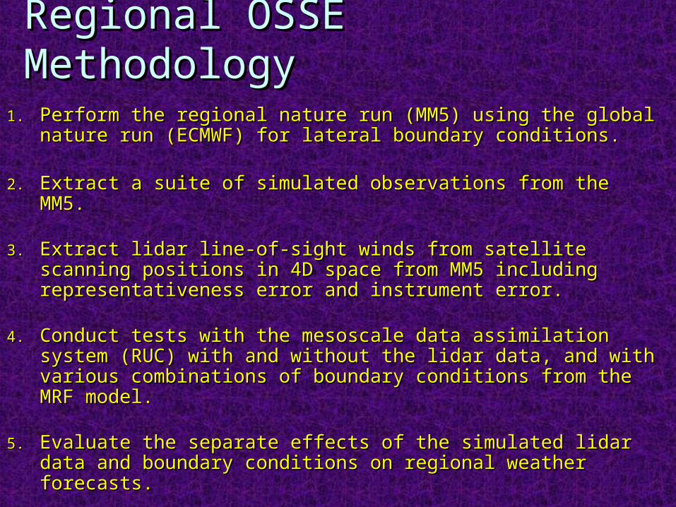
1.1. Perform the regional nature run (MM5) using the global Perform the regional nature run (MM5) using the global nature run (ECMWF) for lateral boundary conditions.nature run (ECMWF) for lateral boundary conditions.

2.2. Extract a suite of simulated observations from the MM5.Extract a suite of simulated observations from the MM5.

3.3. Extract lidar line-of-sight winds from satellite scanning Extract lidar line-of-sight winds from satellite scanning positions in 4D space from MM5 including positions in 4D space from MM5 including representativeness error and instrument error.representativeness error and instrument error.

4.4. Conduct tests with the mesoscale data assimilation Conduct tests with the mesoscale data assimilation system (RUC) with and without the lidar data, and with system (RUC) with and without the lidar data, and with various combinations of boundary conditions from the various combinations of boundary conditions from the MRF model.MRF model.

5.5. Evaluate the separate effects of the simulated lidar data Evaluate the separate effects of the simulated lidar data and boundary conditions on regional weather forecasts.and boundary conditions on regional weather forecasts.

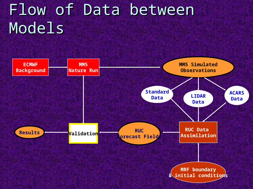
Flow of Data between ModelsFlow of Data between Models

ECMWFBackground

MM5Nature Run

MM5 SimulatedObservations

StandardData LIDAR

Data

ACARSData

RUC Data Assimilation

MRF boundary& initial conditions

RUCForecast Fields

ValidationResults

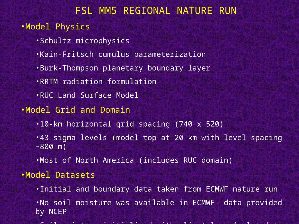
FSL MM5 REGIONAL NATURE RUN

•Model Physics

•Schultz microphysics

•Kain-Fritsch cumulus parameterization

•Burk-Thompson planetary boundary layer

•RRTM radiation formulation

•RUC Land Surface Model

•Model Grid and Domain

•10-km horizontal grid spacing (740 x 520)

•43 sigma levels (model top at 20 km with level spacing ~800 m)

•Most of North America (includes RUC domain)

•Model Datasets

•Initial and boundary data taken from ECMWF nature run

•No soil moisture was available in ECMWF data provided by NCEP

•Soil moisture initialized with climatology (related to USGS landuse)

•Hourly MM5 output (235 GB total) using 36 processors on FSL Jet computer

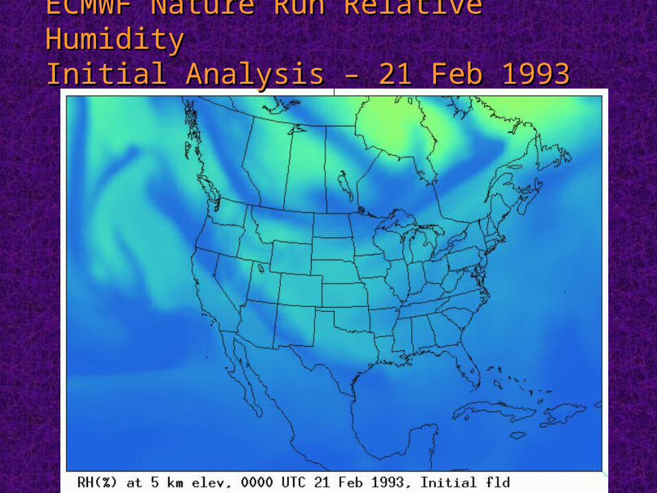
ECMWF Nature Run Relative ECMWF Nature Run Relative HumidityHumidityInitial Analysis – 21 Feb 1993Initial Analysis – 21 Feb 1993

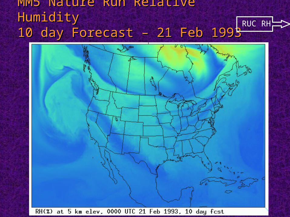
MM5 Nature Run Relative HumidityMM5 Nature Run Relative Humidity10 day Forecast – 21 Feb 199310 day Forecast – 21 Feb 1993

RUC RH

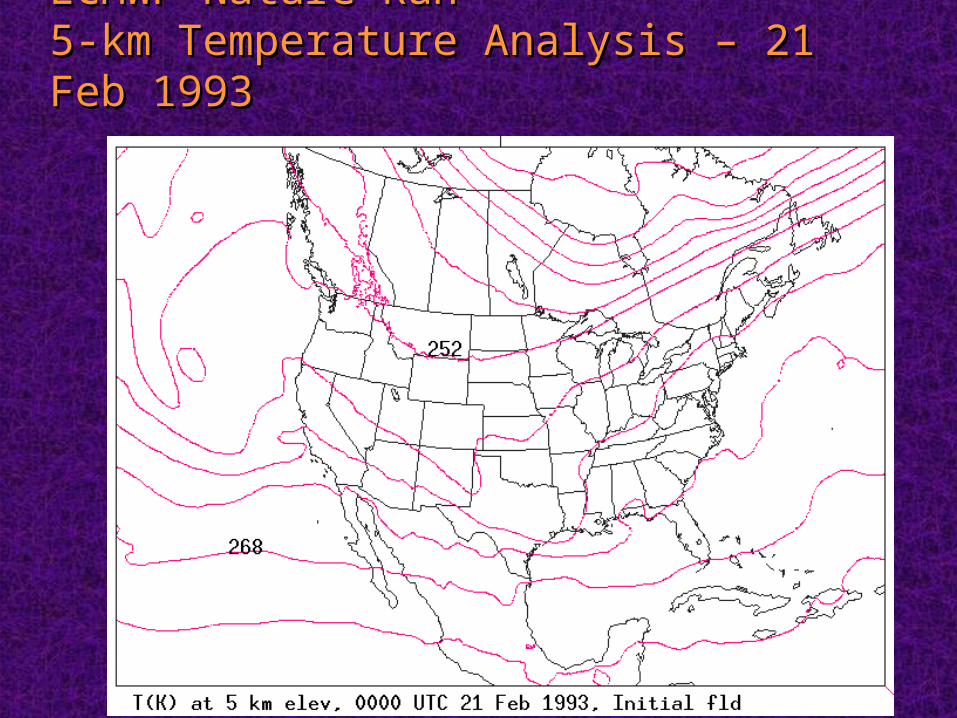
ECMWF Nature Run ECMWF Nature Run 5-km Temperature Analysis – 21 Feb 5-km Temperature Analysis – 21 Feb 19931993

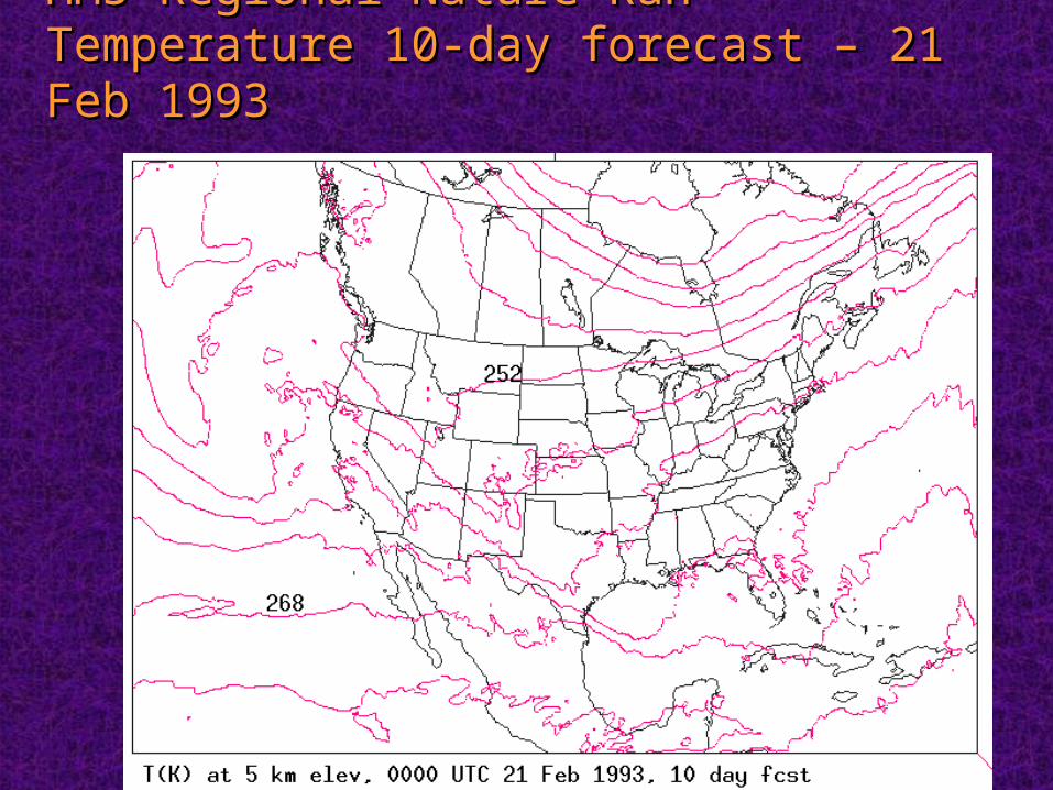
MM5 Regional Nature RunMM5 Regional Nature RunTemperature 10-day forecast – 21 Feb Temperature 10-day forecast – 21 Feb 19931993

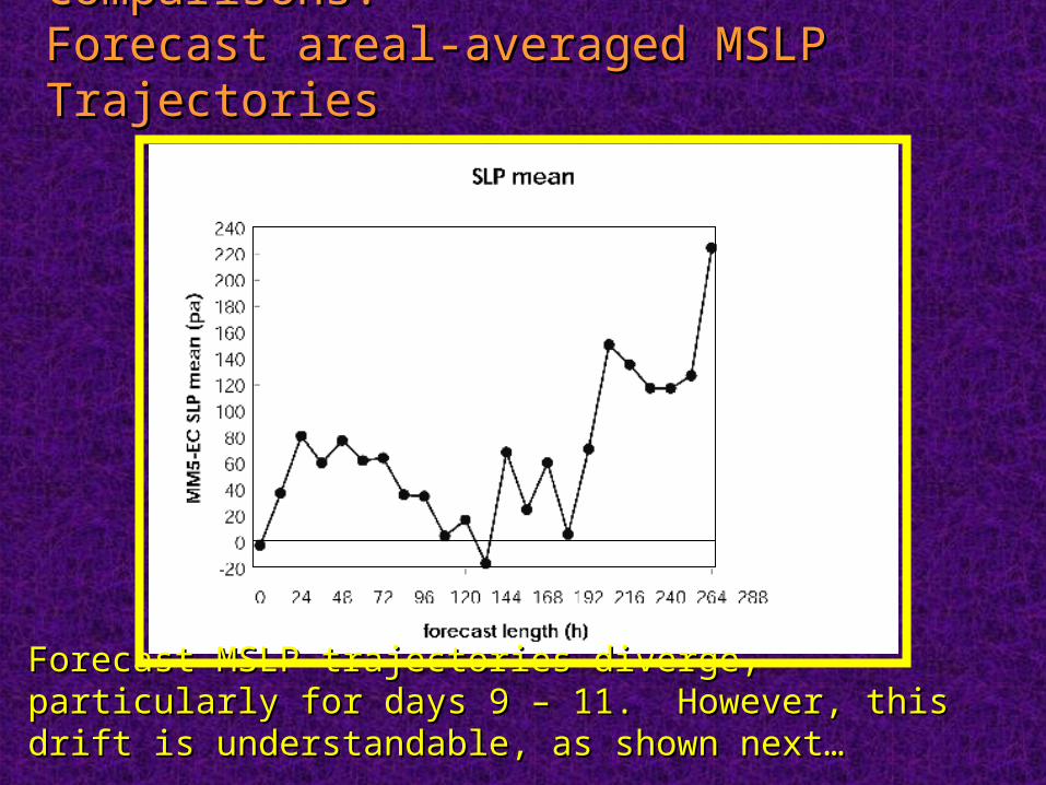
MM5 - ECMWF Nature Run MM5 - ECMWF Nature Run Comparisons:Comparisons:Forecast areal-averaged MSLP Forecast areal-averaged MSLP TrajectoriesTrajectories

Forecast MSLP trajectories diverge, particularly for days Forecast MSLP trajectories diverge, particularly for days 9 – 11. However, this drift is understandable, as shown 9 – 11. However, this drift is understandable, as shown next…next…

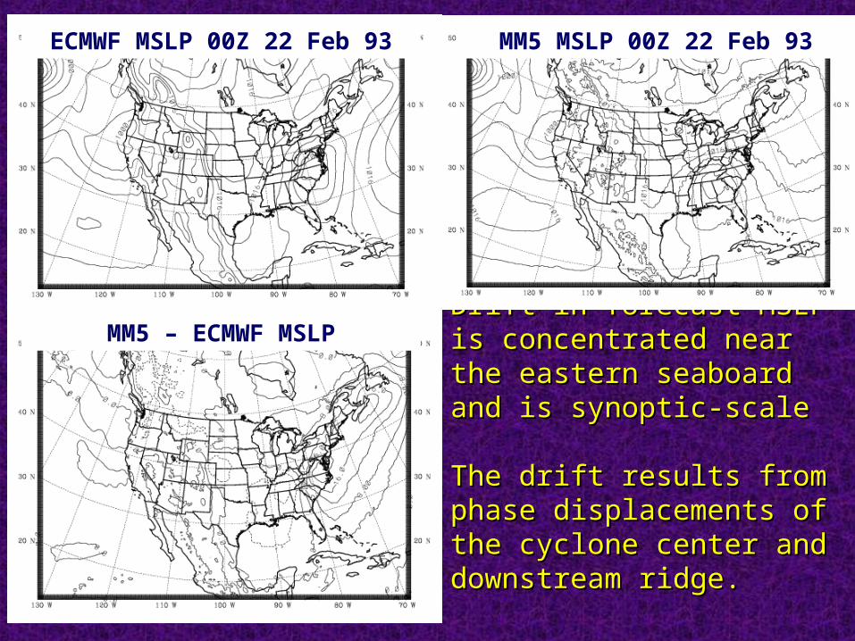
Drift in forecast MSLP is Drift in forecast MSLP is concentrated near the concentrated near the eastern seaboard and is eastern seaboard and is synoptic-scalesynoptic-scale The drift results from The drift results from phase displacements of phase displacements of the cyclone center and the cyclone center and downstream ridge.downstream ridge.

ECMWF MSLP 00Z 22 Feb 93 MM5 MSLP 00Z 22 Feb 93

MM5 – ECMWF MSLP

There is no significant drift in precipitable water.There is no significant drift in precipitable water.

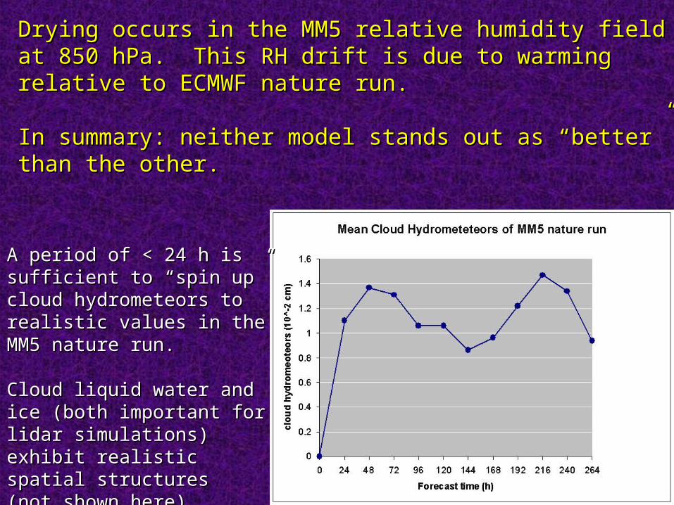
Drying occurs in the MM5 relative humidity field at 850 hPa. This Drying occurs in the MM5 relative humidity field at 850 hPa. This RH drift is due to warming relative to ECMWF nature run. RH drift is due to warming relative to ECMWF nature run.

In summary: neither model stands out as “better” than the other.In summary: neither model stands out as “better” than the other.

A period of < 24 h is A period of < 24 h is sufficient to “spin up” cloud sufficient to “spin up” cloud hydrometeors to realistic hydrometeors to realistic values in the MM5 nature values in the MM5 nature run.run.

Cloud liquid water and ice Cloud liquid water and ice (both important for lidar (both important for lidar simulations) exhibit simulations) exhibit realistic spatial structures realistic spatial structures (not shown here).(not shown here).

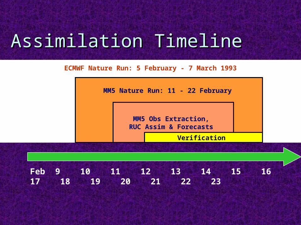
Assimilation TimelineAssimilation Timeline

Feb 9 10 11 12 13 14 15 16 17 18 19 20 21 22 23

MM5 Obs Extraction, RUC Assim & Forecasts

ECMWF Nature Run: 5 February - 7 March 1993

Verification

MM5 Nature Run: 11 - 22 February

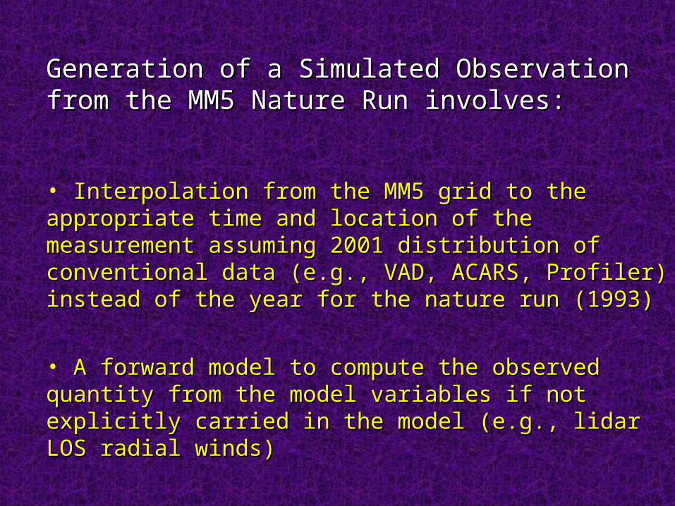
Generation of a Simulated Observation from Generation of a Simulated Observation from the MM5 Nature Run involves:the MM5 Nature Run involves:

• Interpolation from the MM5 grid to the appropriate Interpolation from the MM5 grid to the appropriate time and location of the measurement assuming 2001 time and location of the measurement assuming 2001 distribution of conventional data (e.g., VAD, ACARS, distribution of conventional data (e.g., VAD, ACARS, Profiler) instead of the year for the nature run (1993)Profiler) instead of the year for the nature run (1993)

• A forward model to compute the observed quantity A forward model to compute the observed quantity from the model variables if not explicitly carried in the from the model variables if not explicitly carried in the model (e.g., lidar LOS radial winds)model (e.g., lidar LOS radial winds)

• Specification of error characteristics appropriate for Specification of error characteristics appropriate for the obsthe obs

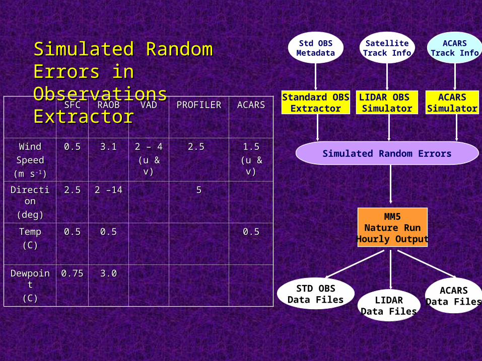
Simulated Random Simulated Random Errors in Observations Errors in Observations ExtractorExtractor

MM5Nature Run

Hourly Output

Standard OBSExtractor

SatelliteTrack Info

LIDAR OBS Simulator

ACARSTrack Info

ACARSSimulator

Std OBSMetadata

STD OBSData Files LIDAR

Data Files

ACARSData Files

Simulated Random Errors

SFCSFC RAOBRAOB VADVAD PROFILERPROFILER ACARSACARS

WindWind

SpeedSpeed

(m s(m s-1-1))

0.50.5 3.13.1 2 – 4 2 – 4

(u & v)(u & v)

2.5 2.5 1.51.5

(u & v)(u & v)

DirectionDirection

(deg)(deg)

2.52.5 2 –142 –14 55

TempTemp

(C)(C)

0.50.5 0.50.5 0.50.5

DewpointDewpoint

(C)(C)

0.750.75 3.03.0

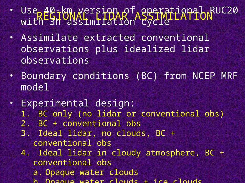
REGIONAL LIDAR ASSIMILATION• Use 40-km version of operational RUC20 with 3h

assimilation cycle

• Assimilate extracted conventional observations plus idealized lidar observations

• Boundary conditions (BC) from NCEP MRF model

• Experimental design:1. BC only (no lidar or conventional obs)2. BC + conventional obs3. Ideal lidar, no clouds, BC + conventional obs4. Ideal lidar in cloudy atmosphere, BC + conventional obs

a. Opaque water cloudsb. Opaque water clouds + ice clouds

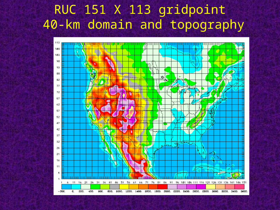
RUC 151 X 113 gridpoint 40-km domain and topography

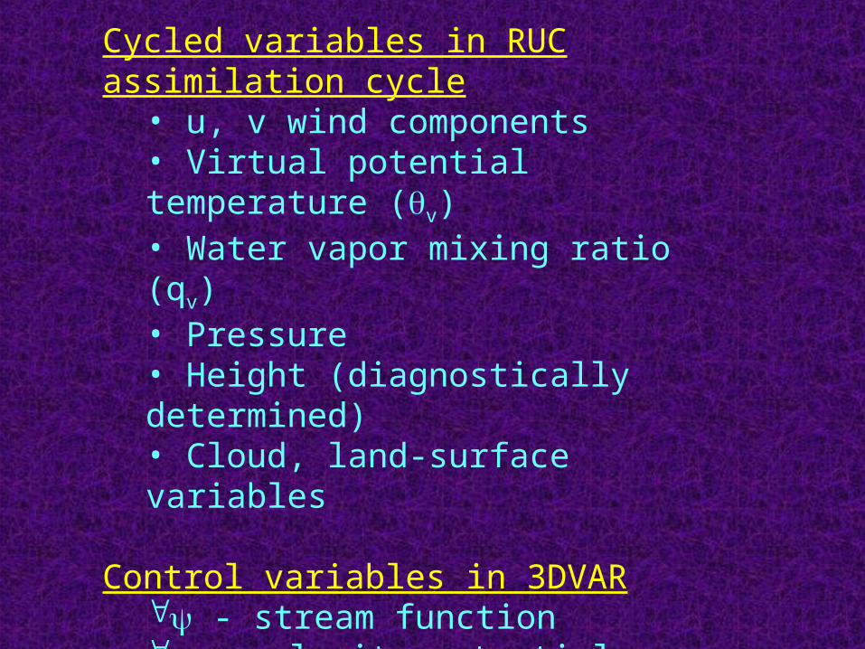
Cycled variables in RUC assimilation cycle• u, v wind components• Virtual potential temperature (v)• Water vapor mixing ratio (qv)• Pressure • Height (diagnostically determined)• Cloud, land-surface variables

Control variables in 3DVAR - stream function - velocity potential•Zunb - unbalanced heightv

•ln (qv )

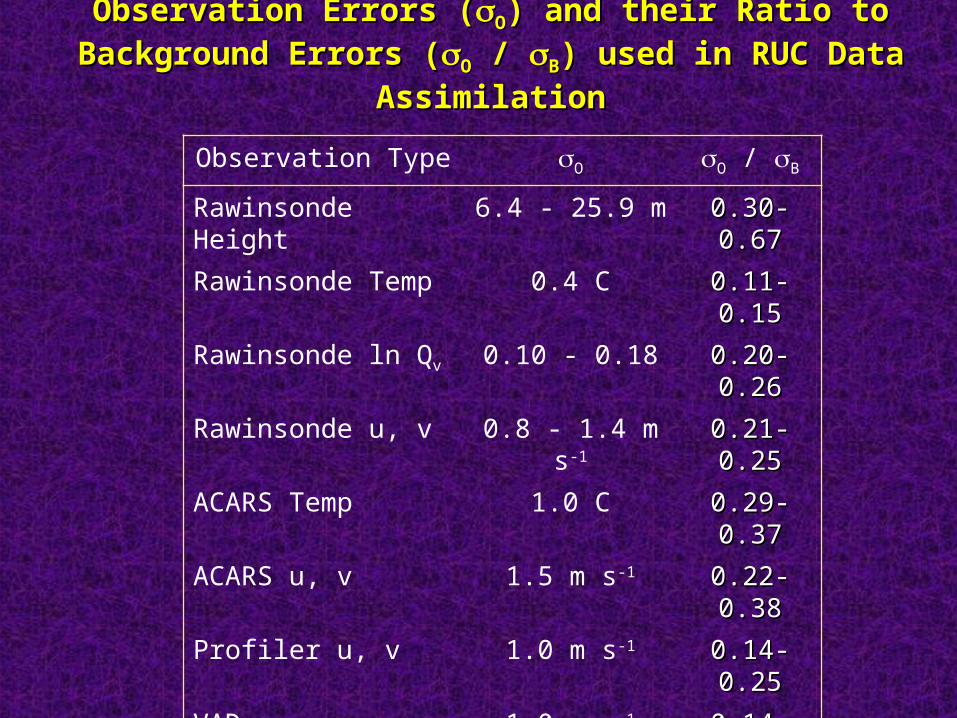
Observation Errors (Observation Errors (OO) and their Ratio to Background ) and their Ratio to Background

Errors (Errors (OO / / BB) used in RUC Data Assimilation) used in RUC Data Assimilation

Observation Type O O / B

Rawinsonde Height 6.4 - 25.9 m 0.30-0.30-0.670.67

Rawinsonde Temp 0.4 C 0.11-0.11-0.150.15

Rawinsonde ln Qv 0.10 - 0.18 0.20-0.20-0.260.26

Rawinsonde u, v 0.8 - 1.4 m s-1 0.21-0.21-0.250.25

ACARS Temp 1.0 C 0.29-0.29-0.370.37

ACARS u, v 1.5 m s-1 0.22-0.22-0.380.38

Profiler u, v 1.0 m s-1 0.14-0.14-0.250.25

VAD u, v 1.0 m s-1 0.14-0.14-0.250.25

Surface u, v 0.5 m s-1 0.130.13

Lidar radial winds 1.0 m s-1

22

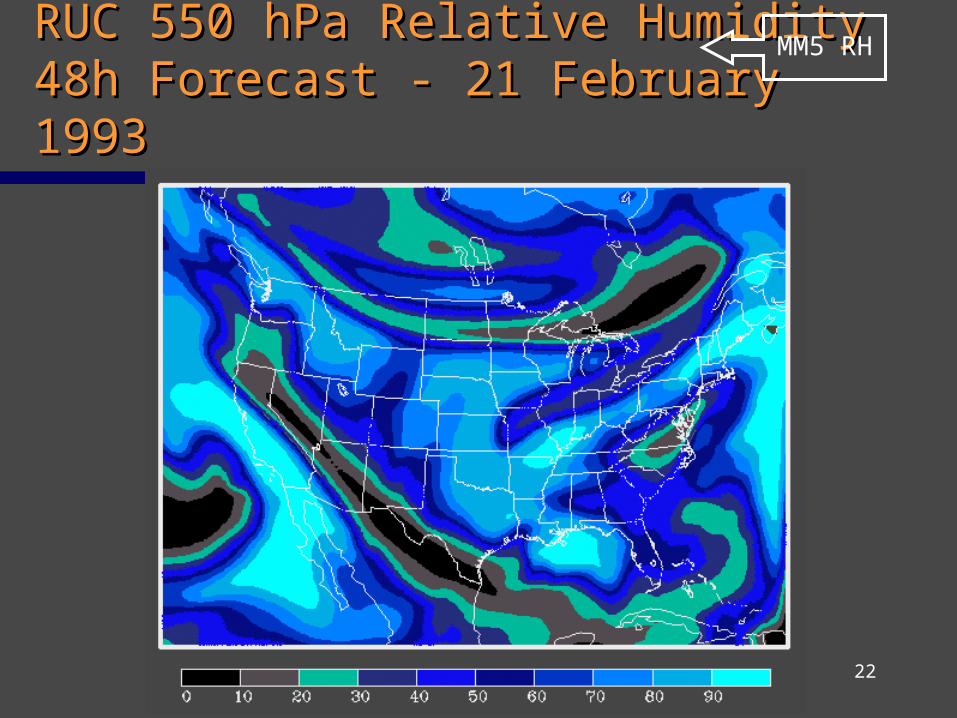
RUC 550 hPa Relative HumidityRUC 550 hPa Relative Humidity48h Forecast - 21 February 1993 48h Forecast - 21 February 1993

MM5 RH

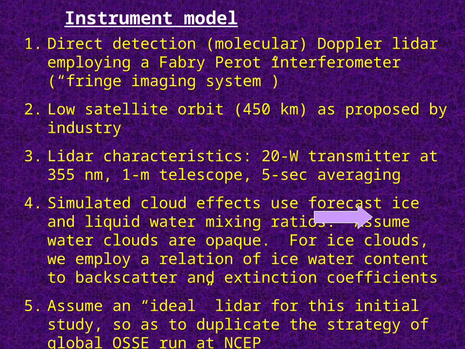
Instrument model1. Direct detection (molecular) Doppler lidar employing a

Fabry Perot interferometer (“fringe imaging system”)

2. Low satellite orbit (450 km) as proposed by industry

3. Lidar characteristics: 20-W transmitter at 355 nm, 1-m telescope, 5-sec averaging

4. Simulated cloud effects use forecast ice and liquid water mixing ratios. Assume water clouds are opaque. For ice clouds, we employ a relation of ice water content to backscatter and extinction coefficients

5. Assume an “ideal” lidar for this initial study, so as to duplicate the strategy of global OSSE run at NCEP

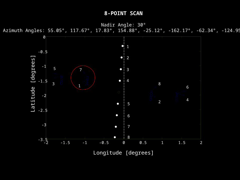
6. Each circular scan is interrupted by 8 “stares” per 1-sec period, consisting of 5 shots averaged over 35 km path

7. Dual-look scanning of the same atmospheric volume

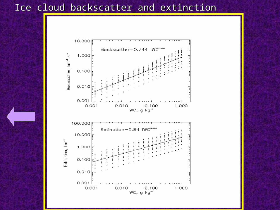
Ice cloud backscatter and extinctionIce cloud backscatter and extinction

3DVAR analyzes horizontal wind: Connection between Global and Regional OSSEs

ECMWF Global Nature Run

GDAS Global OSSE

Experiment

MM5 Regional Nature Run

RUC Regional OSSE

Experiment

Global Regional

Nature Run

OSSE Experiment

Simulated Observations

Boundary Conditions

Boundary Conditions

Simulated Observations

Global Verification

Regional Verification

Griddedoutput

Griddedoutput

Griddedoutput

Griddedoutput

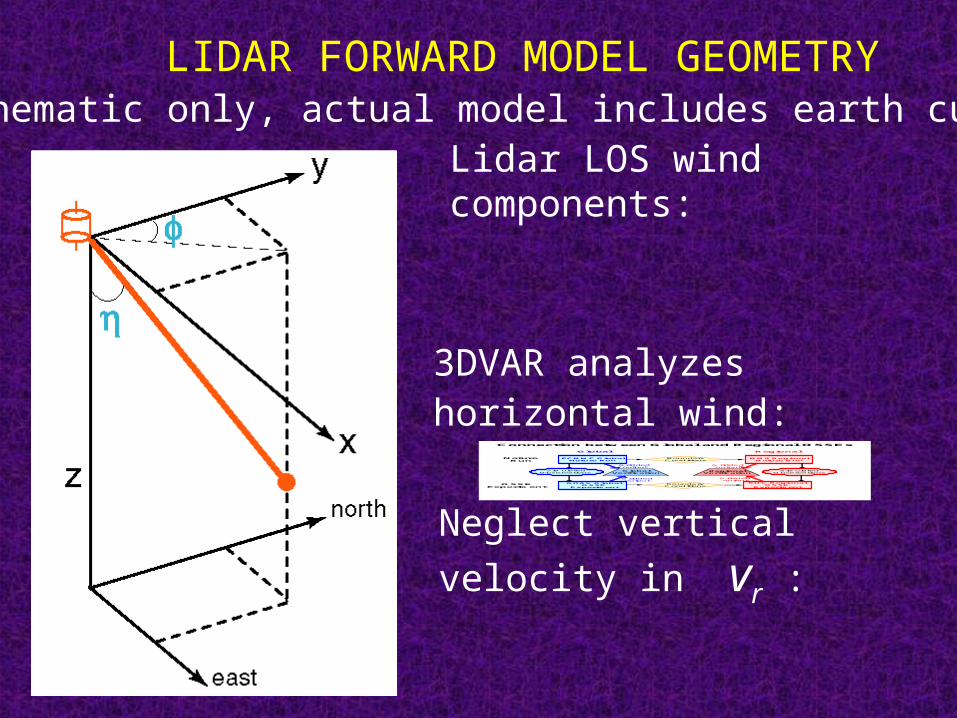
LIDAR FORWARD MODEL GEOMETRY

Lidar LOS wind components:

Neglect vertical velocity in vr :

(schematic only, actual model includes earth curvature)

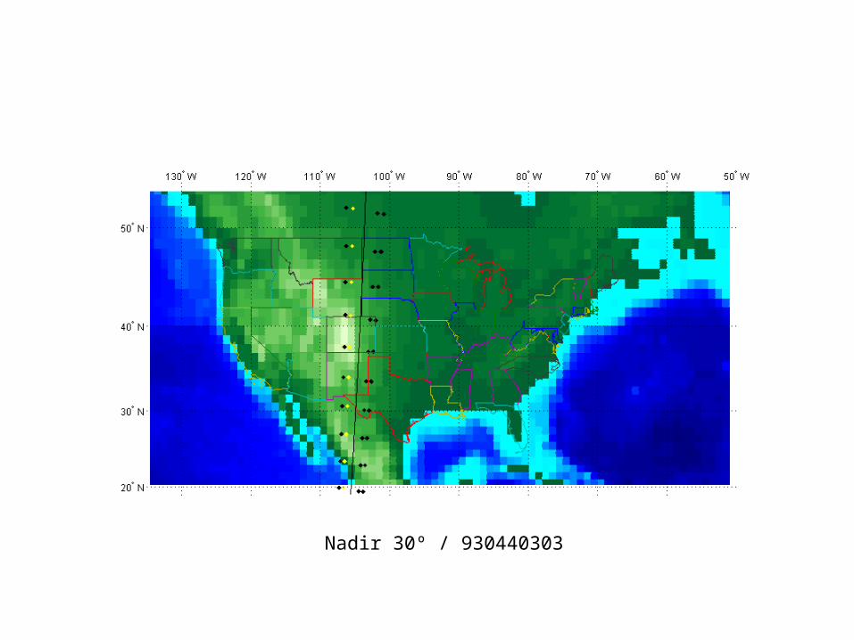
Nadir 30º / 930440303

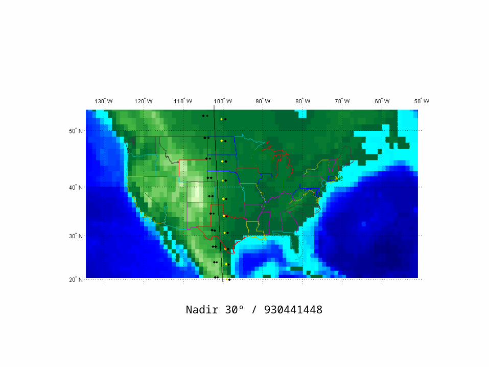
Nadir 30º / 930441448

-2 -1.5 -1 -0.5 0 0.5 1 1.5 2-3.5

-3

-2.5

-2

-1.5

-1

-0.5

0

1

2

3

4

5

6

7

8

1

2

3

4

5

6

7

8

Latit

ude

[deg

rees

]

Longitude [degrees]

8-POINT SCAN

Nadir Angle: 30°Azimuth Angles: 55.05°, 117.67°, 17.83°, 154.88°, -25.12°, -162.17°, -62.34°, -124.95°

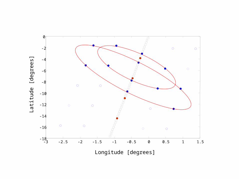
-3 -2.5 -2 -1.5 -1 -0.5 0 0.5 1 1.5-18

-16

-14

-12

-10

-8

-6

-4

-2

0La

titud

e [d

egre

es]

Longitude [degrees]

Remaining TasksRemaining Tasks

Continuous assimilation and forecasts Continuous assimilation and forecasts for test period - compare RUC to MM5 for test period - compare RUC to MM5 nature runnature run

Comparison of LIDAR, no-LIDAR runs Comparison of LIDAR, no-LIDAR runs with control run, including precipitation with control run, including precipitation impactsimpacts

Final Report due 30 September 2002Final Report due 30 September 2002