STATUS OF THE CALIFORNIA SHEEPHEAD (SEMICOSSYPHUS PULCHER) STOCK (2004)

Suzanne H. Alonzo

Center for Stock Assessment Research (CSTAR) and the Institute of Marine Sciences

University of California Santa Cruz

1156 High Street

Santa Cruz CA 95064

Meisha Key

California Department of Fish and Game

20 Lower Ragsdale Dr, Suite 100

Monterey, CA 93940

Teresa Ish

Center for Stock Assessment Research (CSTAR)

Department of Applied Mathematics and Statistics and Jack Baskin School of

Engineering

University of California Santa Cruz

1156 High Street

Santa Cruz CA 95064

Alec D. MacCall

National Marine Fisheries Service

Southwest Fisheries Science Center

Santa Cruz Laboratory

110 Shaffer Road

Santa Cruz, CA 95060

EXECUTIVE SUMMARY ............................................................................................................ 1

1. INTRODUCTION ...................................................................................................................... 3

2. HISTORY OF FISHERY ........................................................................................................... 3

3. BIOLOGICAL INFORMATION ............................................................................................... 7

4. DATA SOURCES AND INITIAL ANALYSIS ...................................................................... 15

5. SINGLE-SEX APPROXIMATION ......................................................................................... 23

7. STATUS OF THE STOCK AND PROJECTIONS ................................................................. 41

8. REVISED MODEL FOLLOWING THE PANEL REVIEW .................................................. 43

9. ACKNOWLEDGEMENTS...................................................................................................... 52

10. REFERENCES ....................................................................................................................... 53

11. TABLES AND FIGURES ...................................................................................................... 59

12. APPENDICIES..................................................................................................................... 146

EXECUTIVE SUMMARY

Stock: California Sheephead (Semicossyphus pulcher) is found along the coast of California

from Monterey Bay southward down into Baja California, Mexico. Sheephead have been fished

recreationally and commercially for most of the last century.

Catches: Post-1950 commercial landings peaked both in the 1950s and the 1990s with

recreational fishing showing an increase in landings in the 1980s and both commercial and

recreational landings have been lower in recent years.

Data and assessment: The California population of California Sheephead was assessed using a

“Stock Synthesis” (hereafter called Synthesis) length-based model. Landings data were

summarized as four distinct fisheries: three commercial fisheries (hook and line, setnet and trap)

and one recreational fishery. Landings data were supplemented by four abundance indices and

length composition data associated with each of the four fisheries. Three of the four abundance

indices were catch per unit effort (CPUE) measures based on landings and effort data from the

California Passenger Fishing Vessel (CPFV) logbook recreational fishery for different time

frames and units of effort. The fourth abundance index was based on the California Cooperative

Oceanic Fisheries Investigation (CalCOFI) larval survey data. Selectivity curves differed among

fisheries and the selectivity of the three CPUE indices from the recreational fishery were

assumed to have the same selectivity as estimated for the recreational fishery.

1

Status of the stock: Changes in the spawning potential ratio based on estimated current and

unfished mature female and male spawning biomass indicates that the stock is below the target

level of 50% of the unfished condition described by the Nearshore Fishery Management Plan

(NFMP). For the most likely scenario, the spawning potential ratio of California Sheephead

(based on mature biomass) has been reduced to 20% of the unfished condition. Application of

the NFMP 60/20 policy indicates that a reduction in allowable catch is warranted.

Recommendations: Data needs include sex-specific age and length records of individual fish

(also by location and fishing depth, if possible) from the recreational and commercial fisheries.

These data are needed to 1) resolve uncertainty about growth rates and the coefficient of

variation in individual size at age; 2) specify current age and lengths at maturity; 3) specify

current age and length at sex change; and to determine the extent of spatial variability in these

life history features. Further refinement of the sex change dynamics and relevant life history

parameters (especially individual variation in growth) would also improve our ability to interpret

the fishery data. Behavioral studies of the effect of removing territorial males and the speed with

which replacement dominant males and harems are re-established would help resolve whether

total fishing closure in some areas is more or less effective than reduced fishing intensity in all

areas. Finally, further information on the abundance and exploitation of Sheephead in Mexico

would improve the ability to assess and manage Sheephead.

2

1. INTRODUCTION

California Sheephead (Semicossyphus pulcher; previously Pimelometopon pulchrum) is in the

genus Labridae. Most species in this genus are small reef fish that are not exploited. In contrast,

California Sheephead can grow to sizes that exceed 80 cm and are found in shallow temperate

waters along the Pacific coast from Monterey Bay, California to Cabo San Lucas, Mexico

(Figure 1.1). In this report, we describe the first quantitative stock assessment of this species

although it has been fished commercially and recreationally for a large part of the past century.

Sections 2 through 7 of this report were prepared prior to a formal stock assessment review, and

are mostly unchanged from the material that was initially presented to the Review Panel. Many

aspects of the assessment model were changed during the review, and the Panel asked for some

follow-up analyses. The final assessment model based on the review is given in section 8, and is

the Assessment Team’s best effort to accommodate the Review Panel’s recommendations.

However, Section 8 itself was not reviewed by the Panel.

2. HISTORY OF FISHERY

2.1 Commercial Fishery: Beginning with the salted fish fishery in the 1800s, California

Sheephead have maintained a presence in the California nearshore fishery. From the early 1920s,

Sheephead sporadically appeared in reported landings for the nearshore fishery, with booms in

harvest from 1927 to 1931, and again from 1943 to 1947, peaking in 1928 at 370,000 lbs.

3

Excluding these periods of high landings, the average annual commercial harvest averaged just

10,000 lbs until the live-fish fishery appeared in the 1980s. The development of this new fishery

corresponded to an upward trend in landings, ultimately reaching a peak of 366,000 lbs in 1997.

During this time, prices, adjusted for inflation, increased from $0.10/lb in the 1940s to 1980s to

over $9.00/lb for live-fish in the 1990s (Stephens 2001).

In just three years (between 1989 and 1992), the nearshore, live-fish trap fishery increased from

2 to 27 boats landing over 52,000 lbs of live fish (Palmer-Zwahlen et al. 1993). Sheephead

accounted for more than 88% of live fish landed in the developing live-fish fishery, which has

greatly contributed to the large increase in total commercial landings. During the early years of

the fishery, commercial hook and line Sheephead landings totaled more than 165,000 lbs, of

which over 66% belonged to the live-fish fishery (Palmer-Zwahlen et al. 1993).

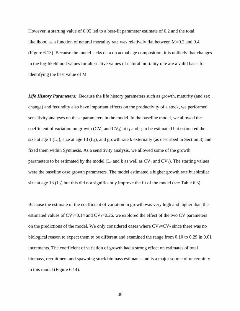
2.2 Recreational Fishery: Sheephead are caught by hook and line as well as by spearfishers

(Young 1973). Landings in the recreational fishery for Sheephead exceeded commercial catch

between 1980 and 1989 (Figure 2.1, Schroeder and Love 2002), and most likely before this as

well, except during the two boom times for the commercial fishery (Palmer-Zwahlen et al.

1993). In 2002, Sheephead ranked 13th in landings in the southern California recreational fishery.

Large, old individuals are especially vulnerable to depletion by recreational spearfishing because

of the ease at which they can be spotted and speared (CDFG 2003).

2.3 Artisanal Fishery: Sheephead represent a large proportion of the artisanal fishery in Baja

California, Mexico, comprising over 25% of the catch, with this proportion increasing in summer

4

months. This fishery is primarily comprised of individuals or small groups fishing with hook and

line on boats less than 8 m long, fishing less than 15 fathoms from shore. The artisanal fishery

tends to be a mixed fishery dominated by Sebastes ssp. In 1994, a study of the artisanal fishery of

the northwestern coast of Baja California (from Santo Tomas to south of Punta Canoas) found

that of 2490 fish caught (representing 2692.7 kg), six hundred forty-five (26%) were Sheephead.

In this sample, the mean standard length of Sheephead was 312.2 ± 56.8 mm (Rosales-Casian

and Gonzalez-Camaho 2003).

2.4 Regulation: Of the 19 nearshore species managed under the Nearshore Fishery Management

Plan (NFMP), 16 (13 species of nearshore rockfish, California scorpionfish, cabezon, and kelp

greenling) are designated as groundfish and fall under the management authority by the Pacific

Fishery Management Council (PFMC). California Sheephead, monkeyface prickleback (also

called monkeyface eel), and rock greenling do not have groundfish designation, thus do not fall

under the management by the PFMC. Furthermore, the PFMC has not actively managed cabezon

or kelp greenling. This lack of PFMC management led to State of California regulations for

California Sheephead, the two greenling species, and cabezon (CDFG 2002). Regulations for

California Sheephead tend to fall under the general nearshore fishery regulations. The

commercial fishery for both trap and hook and line gear is a restricted access fishery. Permits for

the live-fish trap fishery began in 1996 in southern California and a statewide Nearshore Fishery

Permit began in 1999. These permits are limited to individuals who have participated in the

fishery the previous year as well as meeting historical catch criteria.

5

The Sheephead trap and hook and line fisheries reached optimal yield (OY) levels and closed

early for all years, beginning in 2001. According to the NFMP, “Optimum yield (OY) is defined

in FGC §97 as the amount of fish taken in a fishery that does all of the following: (a) provides

the greatest overall benefit to the people of California, particularly with respect to food

production and recreational opportunities, and takes into account the protection of marine

ecosystems, and (b) is the MSY of the fishery, reduced by relevant economic, social, or

ecological factors, and (c) in the case of an overfished fishery, provides for rebuilding to a level

consistent with producing MSY in the fishery (CDFG 2002).” The 2002 OY was set to half that

of total recent catches, and allocated almost 50,000 lbs more to the recreational fishery than the

commercial fishery.

Size restrictions on Sheephead were fairly minimal before 1999 for both the recreational and

commercial fisheries. In 1999, CDFG set the minimum catch size for the commercial fishery to

12 inches (total length) and followed with the same size limit for the recreational fishery in 2001.

To further decrease commercial harvest, the minimum commercial harvest size was increased to

13 inches in 2001. Also in 2001, the 10 fish recreational bag limit was reduced to five (NFMP

Table 1.2-17, CDFG 2002)

In 2002, the Sheephead fishery was aligned with the nearshore rockfish fishery for both the

commercial and recreational fisheries (CDFG 2002). Sheephead are not to be taken

commercially north of Point Conception, Santa Barbara County during March and April, and

south of Point Conception during January and February. This essentially represents a seasonal

closure because the bulk of landings occur south of Point Conception (CDFG 2002). Other

6

season and area closures affecting the Sheephead fishery result from management of the

nearshore fishery. In 2001, taking Sheephead deeper than 20 fathoms in a Cowcod Conservation

Area was banned.

3. BIOLOGICAL INFORMATION

The California Sheephead is a protogynous (female to male) sequential hermaphrodite (Warner

1973; Warner 1975) found near-shore along the Pacific Coast of California and Mexico and into

the Gulf of Mexico (Miller and Lea 1972). Sheephead are generalist carnivores (Cowen 1983)

and feed on species such as mussels (Robles and Robb 1993) and red sea urchins

(Strongylocentrotuys franciscanus) (Tegner and Dayton 1981; Cowen 1983) and may play an

important role in regulating the density of their prey (Cowen 1983; Hobson and Chess 1986;

Robles 1987; Robles and Robb 1993).

3.1 Age and Natural Mortality: Two studies used observed patterns of age structure to estimate

(annual) natural mortality in California Sheephead by assuming age- and sex- independent

mortality. Warner (1975) estimated the annual survival at Catalina Island, California and

Guadalupe Island, Mexico to be approximately 0.7 while Cowen (1990) estimated annual

survivorship in 5 different populations ranging from 0.577 at Guadalupe Island, Mexico to 0.745

at San Nicolas Island, California (see Table 3.1, Figure 1.1). Since the relationship between

mortality rate and survivorship is given by S=e-M (where M is annual natural mortality rate and S

is annual survival), we use M=0.35 as the baseline natural mortality and conduct sensitivity

7

analyses on natural mortality by allowing the parameter to vary ranging from 0.05 to 0.5 in our

assessment. The oldest fish ever reported was 53 years old (Fitch 1974). However, size at age

data based on dorsal spines found fish that were at most 21 years old (Cowen 1990). Therefore

we used the 53-year-old fish to set a realistic lower bound on mortality. Based on Hoenig (1983),

this corresponds with a constant mortality of 0.07 approximately. Thus we use 0.05 as a lower

bound for our sensitivity analyses. The upper bound was determined by the populations with the

lowest observed survival (see Table 3.1).

3.2 Growth: The precise growth patterns as well as size and age distributions of Sheephead in

the wild appear to vary slightly among sites and over time (Warner 1973; Warner 1975; Cowen

1990; DeMartini et al. 1994). The largest individual ever observed was 91 cm (Miller and Lea

1972). DeMartini et al. (1994) found the relationship (R2=0.92 p<0.0001 N=61) between total

length (in inches) LT and wet body weight W (in grams) to be

ln W=ln 0.688 + 2.723 ln LT (3.1)

We used the following relationship from the Recreational Fisheries Information Network

(RecFIN) database to convert total length (LT) in cm to fork length (LF) in cm

LF = -1.4564+1.094 LT (3.2)

8

For our model, we used the power relationship in Equation 3.1 and the length conversion from

Equation 3.2 to calculate the expected relationship (Figure 3.1) between fork length in

centimeters LF and body weight in kilograms W

W=aLFb where a=0.000026935 and b=2.857 (3.3)

Using linear regression, we found the relationship between standard length and total length for

California Sheephead using individual lengths from the Central California Spearfishing

Tournament database (CenCAL, N=100). We excluded one data point because it reported the

biologically impossible situation where total length was less than standard length. This gave the

relationship between standard length in cm Ls and total length in cm LT

LT = 0.604 + 1.207 LS (3.4)

We used the size at age data (converted into fork length using Equations 3.2 and 3.4) for Catalina

Island, California published in Warner (1973) for our baseline estimates and size at age data

from Cowen (1990) for sensitivity analyses on these parameters. Because we did not have any

age data from the fisheries or surveys, we fixed the growth parameters within any single run of

the model rather than allow them to be estimated. However, we performed sensitivity analyses

on these growth parameters as described in greater detail below.

We found the best-fit estimates of growth parameters by minimizing the sum of squared

deviations between the predicted and observed size at age (Hilborn and Mangel 1997). We

9

compared the ability of four different methods of fitting the growth parameters k and Linf to

predict the observed growth data. We first used a Ford Plot (Quinn and Deriso 1999) with an

unconstrained Linf and found the growth parameter k and asymptotic size Linf that best fit the

data. Second, we used a Ford Plot but constrained Linf to be the maximum observed size of 91

cm and only fit the growth rate k. Both of these approaches lead to a good fit between the

predicted change in size between ages and the observed size at age data (SS1=18.68 and

SS2=19.15). Third, we fit the growth rate k using the Schnute (1981) parameterization of the von

Bertalanffy growth equation with an estimated Linf using t1=1, L1=12.92 and t2=13, L2=52.60 cm

fork length (the smallest and largest ages for which a mean size at age was given in Warner

(1975) data). Finally, we fit the Schnute (1981) parameterization with the asymptotic size Linf set

to maximum observed size. The estimated mean size at age predicted from the best-fit growth

parameters using the third and fourth approach did not fit the data well (SS3=1988.71 and

SS4=1687.07). The Ford plot with an unconstrained asymptotic size (predicting the size at time

t+1 from time t) gave the best fit to the observed size at age data and thus we used these

estimates of the growth parameters in the baseline version of the model (k=0.068, Linf=83.86 cm,

Figure 3.2). Although this gave a smaller asymptotic size than the maximum size ever reported,

it was a better fit with the observed size at age data and is consistent with the maximum length of

fish observed in the fisheries (see Section 4). Because Synthesis uses the Schnute

parameterization of the von Bertalanffy growth equation (Schnute 1981; Methot 2000), we used

the parameters t1=1 (years), L1=12.92 (cm fork length), t2=13 (years), L2=52.60 (cm fork length)

and k=0.068 as the baseline values in our model (Figure 3.2). We also used the same method to

find growth parameters for the other populations for which we had data (Warner 1975; Cowen

1990) and used each set of growth parameters (given in Table 3.1, Figure 3.3) in a separate run

10

of the model as a sensitivity analysis on size at age. We also used the error bars in the mean size

at age data given in Warner (1975) to estimate a coefficient of variation in size. The small

sample sizes (N=2 to 12 for each age class) led to a very high estimate for coefficient of variation

of growth per age class (CV=0.3) so we used this value as an upper bound for the Synthesis

model and allowed the model to estimate the coefficient of variation at age (CV1 and CV2).

3.3 Distribution and Abundance: Sheephead are found from Monterey Bay to the Gulf of

California (see Figure 1.1) but are uncommon north of the Point of Conception and are much less

common in the Gulf of California than along the Pacific Coast (Miller and Lea 1972). In the

Channel Islands, densities of 1475-1525 individuals of all sizes per hectare have been observed

(Davis and Anderson 1989) while Cowen (1985) reports densities ranging from 16-290 adult fish

per hectare.

3.4 Dispersal: Tagged adult Sheephead were usually caught again on the same reef (DeMartini

et al. 1994), showed little movement (Davis and Anderson 1989) and a high rate of recapture

(71%, 36 of 51 individuals) (DeMartini et al. 1994). Although weak population structure has

been found between southern California and Baja California, Mexico (Waples and Rosenblatt

1987), the genetic structure is consistent with frequent dispersal among populations, probably at

the early life stages although adults may disperse short distances through deep water. Bernardi et

al. (2003) found no genetic structure between populations of Sheephead both when comparing

Pacific and Gulf of California populations and when comparing California with Mexican

populations along the Pacific coast (FST=0) (Bernardi et al. 2003). Thus, there appears to be high

11

levels of gene flow between populations of Sheephead, at least for evolutionary time scales

(Bernardi et al. 2003).

3.5 Recruitment: Recruitment patterns are temporally and seasonally variable (Cowen 1985;

Cowen 1985; Cowen 1991). Sheephead have a pelagic larval stage prior to recruitment in

shallow waters. Although the pelagic larval duration ranges from 37-78 days, the size at

settlement varies little (range 12.7-16 mm and mean 13.5 mm) and growth after settlement is not

affected by age at settlement (Cowen 1991). A comparison of 9 years of recruitment data found

that recruitment patterns (based on field transects as well as age structure data) are highly

variable but can be related to oceanographic data and proximity to other populations that may

supply larva (Cowen 1985). Cowen (1985) also found a positive relationship between adult

density and recruitment, but did not report any other evidence of density-dependence. Sheephead

larval availability depends on season and peaks July to October and larva are found mainly

nearshore (Cowen 1985).

3.6 Maturity and Sex Change: California Sheephead individuals have been observed to mature

at about 4 years of age and with a mean standard length of 20 cm (Warner 1975) although

individual variation as well as differences among populations exist (Cowen 1990). Sex change

occurs at approximately 30 cm standard length at an age of 7-8 years although it can occur at

standard lengths as low as 18 cm and ages as young as 4 years (Warner 1975; Cowen 1990). The

degree to which sex change is determined by endogenous versus exogenous cues is not known.

However, sex change appears to depend on size rather than age and the size at sex change is

consistent with predictions of the size-advantage model (Cowen 1990). Populations with higher

12

growth rates and higher survival also have larger sizes at sex change and sex ratio seemed to

affect population patterns of sex change as well (Cowen 1990). Warner (1975) reports the

frequency of immature individuals, mature females and mature males at Catalina Island,

California. We used these data to find the L50 (length at which the proportion mature or male is

50%) for maturity and sex change. We then fit these data to a logistic function estimating the

slope parameter that minimized the sum of squared deviations between the predicted and

observed proportion of mature individuals and the proportion of mature individuals that are

female for use in the model. We used the parameters based on the Catalina Island data for our

baseline model and use the other maturity and sex change parameters for sensitivity analyses

(see Table 3.1, Figure 3.4).

3.7 Fecundity: Reproduction occurs June through early October, while sex change occurs during

the winter months (Warner 1975; Cowen 1990). Females appear to spawn multiple times during

the reproductive season. DeMartini et al. (1994) estimated that females spawn approximately 86

times per year (about every 1.3 days) and calculated the batch fecundity of females to be 5755

eggs per spawning event, but found no significant relationship between the number of eggs

released per kilogram of body weight and total female body weight (an average of 15 eggs per

gram of body weight or 15,000 eggs per kg, DeMartini et al. 1994). From these data, we estimate

both the total egg production of a female based on her weight (Figure 3.5 dashed line) as well as

the annual total egg production per kilogram of female body weight (batch fecundity per kg and

number of patches per year, Figure 3.6 dashed line).

13

Warner (1975) found that the ovary weight (OW in grams) of females scaled with standard length

(L in cm) according to

OW=0.00131 L2.95 (3.4)

Warner (1975) also found that on average females have 5377 yolky oocytes per gram of female

gonad. Thus it is also possible to estimate the total and mass-specific egg production from

Warner (1975) and the weight-length relationship given in Equation 3.3 (Figures 3.5 and 3.6).

The difference in the exponents between Equation 3.3 and 3.4 imply that a weak increase in

mass-specific egg production is predicted (Figure 3.6). However, in the weight and size range in

which individuals are actually expected to be female, the relationship is nearly linear.

Furthermore, one set of data measured the number of eggs being spawned while the other

counted the number of oocytes in the gonad. These lead to slightly different estimates of total

egg production. However, the general functional form is basically the same (Figures 3.5 and 3.6).

Since the number of eggs actually spawned by females is a better estimate of total egg

production, we used the DeMartini at al.(1994) based estimates of fecundity for our baseline

version of the model. However, we explored the effect of the lower oocyte production from

Warner (1975) as one of our sensitivity analyses.

Nothing is known about fertilization rates or sperm production in California Sheephead. At high

fishing mortality, the potential for sperm limitation exists since fishing may remove large males

preferentially (Alonzo and Mangel 2004). However in Sheephead, large males may experience

sperm competition from smaller males (Adreani et al. In Press) and thus sperm production may

14

be high in this species (Birkhead and Møller 1998) making the species less prone to sperm

limitation.

4. DATA SOURCES AND INITIAL ANALYSIS

4.1 Fishery Catch Data: We divided the catches into four separate fisheries, three commercial

and one recreational. The commercial fishery was divided by three gear groups: hook and line,

trap and setnet. We attributed all commercial landings to the hook and line fishery prior to 1978,

when the Pacific States Marine Fisheries Commission (PSMFC) began a sampling program so

catch could be estimated by gear. The recreational catch is landed primarily by the Commercial

Passenger Fishing Vessel (CPFV) fleet. Logbook-based catch estimates consistently began

around 1947. Table 4.1 summarizes commercial (by gear) and recreational catch used in this

assessment.

Commercial Catch: Commercial landings date back to 1916 and come from three sources. We

used landings from 1916 – 1977 that were reported in California’s Living Marine Resources: A

Status Report, which include landings brought into California from Mexico. We did not have

catch data for any other fishery prior to 1947, so we calculated the mean catch from 1937-1946

(55.47 metric tons, assumed all hook and line) for the historical catch value used in the baseline

model.

15

We obtained the estimated catch by gear for 1978 – 2003 (1980 data missing) from the

California Cooperative Survey (CALCOM) database (Brenda Erwin, Pers. Comm.). Expansion

procedures were used to estimate commercial catch from sampling commercial market

categories (Pearson and Erwin 1997). The Sheephead market category is fairly clean, which

makes estimating catch for Sheephead more precise than for other species (e.g. rockfish). Catch

for trawl, miscellaneous and unknown gears were low and were allocated proportionally to the

annual landings of the other gear groups. All commercial landings were converted from pounds

to metric tons. During the 1980s some Sheephead were landed under the “miscellaneous

rockfish” market category (Chris Hoeflinger, Pers. Comm.). This practice was not detected by

the limited amount of port sampling at that time. The contribution of “miscellaneous rockfish”

landings to Sheephead catch is treated as negligibly small in this assessment.

We considered three other sources of commercial landings for this assessment: Pacific Coast

Fisheries Information Network (PacFIN), Pacific Fisheries Environmental Laboratory (PFEL)

and the Commercial Fisheries Information System (CFIS). We found no significant differences

in the overlapping time periods for all available sources (Figure 4.1a). We therefore used the

CFIS estimates (also separated by gear) to fill in for the 1980 missing year in the CALCOM data.

We also compared sources that included catch brought into California from Mexico. PFEL

reports landings not including Mexico catch beginning in 1928. California’s Living Marine

Resources: A Status Report includes Mexico catch beginning in 1916. The landings between the

two sources from 1928-1977 showed no significant difference (Figure 4.1b).

16

Recreational Catch: Recreational catch estimates came from two sources. We obtained

recreational landings in numbers of fish from 1947-1979 for the Commercial Passenger Fishing

Vessel (CPFV) fleet from historical Department of Fish and Game (DFG) Fish Bulletins. We

converted numbers of fish to metric tons using an average 3.1 pounds per fish (Young 1969).

Landings were also inflated to account for recreational dive take and discards. We estimated dive

removal to be 2700 fish per year (Young 1973) and applied this back to 1955, which is

approximately the time SCUBA began. Discards were estimated by using the mean discard rate

(15%) for 1980-1989 from the Recreational Fisheries Information Network (RecFIN). We

compared this rate to the logbook discard information from 2000-2003, which was also 15%.

In 1980, the Marine Recreational Fishing Statistical Survey (MRFSS) began sampling, and from

1980-2003 (with a hiatus from 1990-1992) estimated landings, effort and discards are available

from the RecFIN website. We increased the RecFIN estimated landings by an additional 3.84

metric tons per year (an average 2700 fish per year at 3.1 pounds per fish) to account for the

estimated dive take. For the years 1990-1992, we used the landings data from the DFG Fish

bulletins and estimated catch (including dive) and discards as described above for the 1947-1979

time period.

We did not include the removals of Sheephead taken by spearfishing in this assessment for two

reasons. To calculate dive take we used an estimated 3.1 pounds per fish (Young 1973), which

would underestimate removals with this gear in the model, considering they target larger fish. If

the 3.1 average sized fish were used, that would account for an additional 0.043 metric tons a

year, which is minor. We concluded there was not enough information to identify Spearfishing

17

as its own fishery. Secondly, these fish were speared in Central California, and we focused our

assessment on the Southern California population.

4.2 Abundance and CPUE: We used four surveys in this assessment, one to produce an index

of larval abundance and three to produce indices of catch per unit effort (CPUE) in the

recreational fishery.

CalCOFI Larval Survey: To create an index of larval production for Sheephead, we used the

California Cooperative Oceanic Fisheries Investigations (CalCOFI) data (Richard Charter, Pers.

Comm.). These data have been collected in most years since 1951, and are used to track trends in

larval production in southern California and Mexico (Moser et al. 2001).

The initial analysis began with manta and bongo tows pertaining to southern California and

Mexico (lines 77-120), with all stations and months included. We used data from the typical

Sheephead spawning season (June through October). If less than 5 larvae were examined in the

survey over all years in a single month, those months were excluded from our frame. Station

numbers greater than 65 were excluded, since no larvae were found outside of the nearshore

area. Subsetting this dataset resulted in some years being excluded from the analysis, where in

other missing years, surveys were not attempted at all.

We ran this subset of CalCOFI data through a delta-lognormal Generalized Linear Model (GLM)

with year, month and station effects (Stefansson 1996). The spawning output index and catch are

18

variable from year to year (Figure 4.2). Several years had only one positive tow with Sheephead

larvae, so we could not jackknife estimates of precision (at least two are needed).

Recreational Catch per Unit Effort (CPUE): Beginning in 1936, CPFVs were required to turn

in a daily log, reporting the number of anglers aboard as well as the total catch in numbers of fish

by species. Due to World War II, there was a delay in recreational fishing and partyboats did not

begin turning in the mandatory logs and reporting catch consistently until 1947. Initially, effort

was reported in angler days, which switched to angler hours in 1960. Recreational catch and

effort data were taken from 2 sources: CPFV logbooks reported in Fish and Game Bulletins

(1947-1979) and logbook block data provided by the Department of Fish and Game (1980-2003)

(Wendy Dunlap, Pers. Comm.).

We separated the CPFV logbooks reported in Fish and Game Bulletins into two time periods due

to differing units of effort. From 1947-1961, we used catch per angler day and from 1960-1981

we used catch per angler. We did not use angler hours due to missing angler hour information

from 1977-1981. We also investigated converting the earlier CPUE estimates in units of angler

days to anglers (1.216 conversion factor) for a one-unit time series from 1947-1981 (Figure 4.3).

There were differences in the 1947-1961 time period based on the differing units of effort

(p=.004), but they showed similar trends. After running a sensitivity analysis on the one-unit

time series CPUE (which did not affect the outcome), we felt that using the separate two-unit

time series for CPUE would avoid additional uncertainty error. In all cases, the model is more

tenuous in the earlier years.

19

The third CPUE index (catch per angler hour) was calculated using block data from CPFV

logbooks for the time period 1980-2003. In the initial analysis of this time series, we calculated

an index for the entire area with all blocks included using 1980-1994 data (data available at the

time). We ran a delta-gamma GLM with year, month and block effects (Stefansson 1996). We

found that 70% of the cumulative sum of block values came from 40 individual blocks. We

limited further analysis to these 40 blocks because the GLM assumes a proportional change is

equally meaningful in all blocks. This assumption seems to be better met for those blocks in

which Sheephead are most abundant.

We charted the top 40 blocks and came up with 5 distinct geographic fishing areas: the Channel

Islands (including San Miguel, Santa Rosa and Santa Cruz Islands), San Nicolas Island, Santa

Catalina Island, San Clemente Island and the Banks (Tanner and Cortez) (Figure 4.4a). We

found each area had different seasonal and annual patterns (Figures 4.4 b & c) using all data

from 1980-2003 (once available) so we ran five separate delta-gamma GLMs to estimate a local

index value for each area (Ij). To estimate precision, we used the jackknife function so there

would be a variance associated with each index in each area. We assume the local index

represents the density of fish in each area and that blocks (nj) are of equal area. The population of

fish is proportional to the product of density and area. The combined index, I, is

∑= )( jj nII (4.2)

20

Similarly, we estimated the variance for the combined index using combined variances:

))var(()( 2∑= jj InIVar (4.3)

Figure 4.4d represents the combined catch per unit effort index for the 5 geographic areas in the

southern California CPFV fishery from 1980-2003, reconstructing the population as a whole.

We further analyzed a sixth nearshore area and the catch per unit effort was so small that it did

not affect our previous analysis.

The reduction in bag limit enacted in 2002 probably had a small effect on CPUE. Based on bag

size compositions from 1998 to 2001, truncating bags larger than five down to five fish results in

a 2.5% reduction in CPUE (indicating that the 2002 and 2003 CPUEs might be a slight

underestimate of abundance). The actual reduction is smaller than this because of sharing over-

limit catches with other fishermen (“bag-sharing”) and because bag composition in 2002 and

2003 indicate that the limit was not strictly enforced. No correction for the change in bag limit

was made in this assessment. Overall, the results of regulations from management in recent

years (bag limits, trip limits, mesh size in the trap fishery) should be further analyzed once there

is enough information to detect the impacts.

4.3 Fishery Length Composition Data: Length compositions came from many sources,

commercial and recreational. Since all length composition data were reported in either fork

length or total length (mm), we converted all lengths in the model to fork length using the

conversion equation provided by RecFIN (see Equation 3.2). Once converted to fork lengths

21

(cm), we set up 2 cm bins to calculate length compositions, starting at 18 cm. We did not have

any size at age data above 50 cm, so all lengths 50 cm or larger were binned together in the 50

cm bin. We excluded any length compositions in which five or less individuals were sampled per

fishery in a given year. If more than one data source covered any one year, the source with the

largest sample size was used. Table 4.2 summarizes sample sizes available and used for the

baseline model. Length compositions for each fishery are shown in Figures 4.5 a-d.

Commercial Lengths: We obtained fork length compositions for commercial landings from two

sources. The CALCOM sampling database covered years 1993-2003 (no data in 1994). Average

lengths of Sheephead were fairly similar over the years in the hook and line (49.9 cm) and trap

fisheries (51.5 cm). We did not use the CALCOM lengths for trap gear because only one or two

samples were taken in each year; however, CALCOM is our main source for lengths in the hook

and line fishery (n=107).

The second source used for commercial lengths were from the Archive Market Data provided by

the Department of Fish and Game (Steve Wertz, Pers. Comm.). Sheephead did not appear in the

dataset until 1993, and lengths were available for most years from 1993-2003. All trap lengths

used came from this data set (n=1064) as well as the lengths from the setnet fishery (n=58).

Recreational Lengths: There were more data on length available from the recreational fishery

than for the commercial fishery. We used CPFV length information from RecFIN and two CPFV

sampling programs conducted in southern California during the 1970s and the 1980s. The length

information from Central California (CenCAL) Spearfishing Tournament was also evaluated

22

(Dave VenTresca, Pers. Comm.). We chose not to use this source because they represent large

targeted Sheephead in Central California, and this assessment is focused on the Southern

California population.

We generated recreational length compositions (n=2849) for CPFVs from 1980-2003 (no data

1990-1992) through RecFIN. The peak frequency of Sheephead lengths sampled on CPFVs

centers around 30cm (fork length) with 88% of all measured fish ranging between 22 and 44 cm.

We assumed all fish measured were landed with hook and line.

We also used Sheephead length compositions collected from two southern California CPFV

sampling programs. The first program sampled from 1975-1978 and 1683 Sheephead were

measured (Collins and Crooke In prep.). The second sampling program was conducted from

1984-1989 (Ally et al. 1991) where 3472 Sheephead were measured. The average size of fish

landed from 1975-2003 (no lengths in some years) is variable throughout the time period

(Figure 4.6).

5. SINGLE-SEX APPROXIMATION

Most stock dynamic models either assume that population production scales with mature adult

biomass or that individual fecundity increases (monotonically) with length or age. However, in a

protogynous species, as individuals grow older and larger they change from female to male and

thus traditional combined-sex models will overestimate the production of eggs at the population

23

level. Similarly, traditional split-sex models (that assume males and females can occur in all age

classes) cannot readily incorporate the absence of males in early age and size classes and the

predominance of males in later ages and larger sizes. It is certainly preferable to consider the

existence of sex change when relating spawning stock biomass and production to recruitment,

abundance and landings.

We therefore developed, for the first time, a combined-sex (or single-sex) stock assessment

model that includes a dome-shaped maturity function that incorporates both maturity and sex

change. To confirm that the predicted population dynamics would be unaltered by combining sex

change and maturity, we created two separate, parallel models. First, a split-sex sex-changing

population where individuals are born female and mature and become male with a certain

probability (Alonzo and Mangel 2004). Second, a combined-sex model that considers individuals

starting at the same initial size as the split-sex population where cohort fecundity declines,

simulating the sex change from female to male.

5.1 Model Description: We developed identical two-sex (i.e. sex-changing) and single-sex (i.e.

combined-sex) models, where the sole difference between the two models resides in the maturity

and fecundity functions. For growth, maturity, fecundity and mortality, we used the same

parameters described in Section 3 and given in Table 3.1, see Table 5.1 for all model parameters.

Both models use the difference equation-version of the von Bertalanffy growth equation

(Equation 5.1, Figure 5.1 Gulland 1983) for length and weight estimates where L(a)

( ) ( ) ( )( ) ( )( )( ) ( )d

gg

acLaW

kLkaLaL

=

−−+−=+ ∞ εε expexp1expexp1 (5.1)

24

is the length at age in cm, k is the growth rate, εg is the normally distributed uncertainty term for

the growth rate, L∞ is the asymptotic size in cm, W(a) is at age in kg, and c and d are the length-

to weight multipliers. In the weight equation and all subsequent equations, length-at-age is

suppressed to age. In both models, mortality is autocorrelated and varies annually, where ρ is the

autocorrelation parameter and εm is uncertainty

M t +1( )= ρM t( )+ 1− ρ2εm . (5.2)

We assume that sex does not affect growth, so we used the same size-based fishery calculations

for both models. Fishing selectivity for fishery i, θi (Figure 5.2 Methot 2000), is a length-based,

four- parameter double logistic where β1 is the steepness parameter

θi a( ) = pr capture{ }i = Ti

1+ exp −β1 iL − β2 i( )( )( )1+ exp β3 i

L − β4 i( )( )( ) where i =1,2...n (5.3)

of the ascending side, β2, in our case, a length, is the midpoint of the ascending side, β3 is the

steepness parameter of the descending side, β4 is the midpoint of the descending side, also a

length in cm, and Ti is the scaling factor (Methot 2000). We specify two different hypothetical

fisheries with different θi and effort, Ei, for each fishery, loosely based on size composition of

landings from the data. Total fishing mortality, F, for each size-at-age is

F a( )= Eiθi a( )∑ . (5.4)

25

We calculated annual catch, Ci, for each fishery, i, for the single-sex and sex-changing models

whose total populations are represented interchangeably as N(a,t) in equation 5.5 with

observation error, εf.

Ci t( )= Ni a, t( ) 1− exp M t( )− F a( )( )( ) Eiθ i

M t( )( )+ F a( )ε f

a∑ (5.5)

5.2 Creating the Single-Sex and Two-Sex Models: Because Sheephead are protogynous

sequential hermaphrodites, fecundity estimates in the form of egg production must include not

only the proportion of the female population becoming mature, but also the loss of females as

mature females become male. We chose to capture this in two ways: 1) as a single-sex model

where the entire population is female and the fecundity for each age class is determined by the

proportion of the age class that is reproductive as females and 2) as a sex-changing model where

the fecundity for each age class is determined simply by the number of females that are mature

and the number of females is reduced as females become male. In the sex-changing model, all

individuals recruited to the population as females, and became mature with a probability at each

length-at-age, then became male with a different probability at each length-at-age, (Figure 5.3)

pm a( )= 11+ exp r L − L50m( )( ) (5.6)

represented by pf(a) in an equation similar to Equation. 5.6, with r determining the rate of

maturity between lengths and is the length at which half the length class is mature. Because m

L50

26

population size is represented in the single-sex approximation as only female, a single equation

had to encapsulate maturity and the switch from male to female. We adjusted the probability of

maturity based on the conditional between becoming male given that an individual is a mature

female (Equation 5.7).

ps(a) = pm (a)pf (a) (5.7)

Since a portion of the mature females transition to males, the total proportion of mature females

in the cohort declines independently, resulting in a decrease in the number of individuals who

can produce eggs for that cohort (Figure 5.4).

We determine the number of eggs produced, ϕ (Equation 5.8), from a relationship

ϕ(a)sex changing = σNfemale a,t( )pm (a)W a( )ϕ(a)single sex = σN a,t( )ps(a)W a( )

(5.8)

between body weight, W(a), and fecundity where σ is the eggs/kg multiplier. We calculate the

total number of eggs for the age class by multiplying the estimated number of eggs produced by

the size of the age class, N(a,t), and the proportion of the age class that is mature or producing

eggs. We use the Beverton-Holt recruitment (Mace and Doonan 1988; Dorn 2002) where total

recruitment is given by equation 5.9 and h is the steepness parameter, ϕ is the total number of

eggs produced used in place of spawning stock biomass, R0 is virgin recruitment, and φ0 is the

measure of virgin eggs per recruit and εr is process uncertainty in recruitment:

27

( ) ( ) ( )

( ) ( ) ( ) r

a

a

r

a

a

ahhR

ahRtN

ahhR

ahRtN

εϕφ

ϕ

εϕφ

ϕ

∑∑

∑∑

−+−=+

−+−=+

sex single00

sex single0

changingsex 00

changingsex 0

female

)(2.012.0

)(8.01,1

)(2.012.0

)(8.01,1

(5.9)

We use an age-structure model to generate population dynamics. In the sex-changing model,

males and females must maintain separate population dynamics, with individuals within each age

class leaving the female population with a certain probability to join the male population

(Equation 5.10a). The single-sex model (Equation 5.10b) uses a single population

( ) ( ) ( )( )( ) ( ) ( ) ( )( )( ))(1,,)()(exp1,1

)(,)()(exp1,1

femalemalemale

femalefemale

aptaNtaNaFtMtaN

aptaNaFtMtaN

f

f

−+−−=++

−−=++ (5.10a)

N a + 1, t + 1( )= exp −M(t) − F (a)( )N a, t( ) (5.10b)

to represent both the male and female populations.

Both models produced identical results without stochasticity (Figure 5.5) and identical long-term

averages with stochasticity in population size as well as catch yields. Combining sex change and

maturity into a single fecundity equation did not change the population dynamics, as long as the

order of maturity, sex change, reproduction, and mortality were correct.

28

6. STOCK SYNTHESIS MODEL

6.1 Model description: We used the size- and age-structured version of the “Stock Synthesis”

program, hereafter referred to as Synthesis, (Methot 1990; Methot 1998; Methot 2000) to model

the population dynamics of the California Sheephead stock. Synthesis is an age and size-

structured model that projects the survival, growth and reproduction of individual age classes.

Synthesis can incorporate ageing errors and individual variation in growth. Synthesis has three

main components: First, the population model is used to project the size and age structure.

Second, an observation model uses data inputs (in our case landings, CPUE data, survey

information and length compositions, see Section 4) and selectivity functions (logistic functions

with potentially both ascending and descending components) to relate the simulated population

to the data. Third, a statistical model uses a likelihood approach to estimate the best-fit

parameters for the model. Synthesis allows a variety of data types to be combined and used to

estimate parameters in one formulation. A single log-likelihood function is used to calculate the

total log-likelihood value associated with the model and allows emphasis factors to control the

weight of each type of data and parameter in influencing the total likelihood. The likelihood

calculation of our model assumed a multinomial error structure for the length compositions and

log-normal error for the surveys. For more details see Methot (2000).

The preexisting version of Synthesis was not able to incorporate the sex-changing life history of

Sheephead. As described above, the population dynamics of Sheephead can be approximated by

a combined-sex model with a double logistic maturity function (where only individuals that are

mature and female produce eggs, see Section 5). We therefore used a version of Synthesis

29

modified by Rick Methot to allow the maturity function to have both ascending and descending

portions of the equation (synl32r.exe, 1251 KB in size, compiled April 5, 2004). There were 4

parameters associated with the maturity function (see Table 3.1); these gave the probability of

being mature and being female (i.e. the probability of producing eggs). We assumed that

spawning occurs in June for the model, the maximum age class in the model is 20 years of age

(an accumulation ages, accounting for all older fish), and mortality rates are time- and age-

independent. For the original runs of the model we assumed equal likelihood weights (of 1.0) for

all data sources (landings of the four fisheries, length compositions of the four fisheries, three

CPUE indices and the CalCOFI survey). We used a convergence criterion of 0.001 log-

likelihood units for all runs of the model.

Because CPUE data were only available starting in 1947, the landings data described above were

used to generate a landings record from 1947-2003, as well as to estimate historical catch prior to

1947 (see Section 4 for details). Therefore, we used the model to project the population size

structure and abundance during these years. The landings data were used within the model to

estimate fishing mortality and the model assumed that mortality is independent between the four

fisheries (hook and line, setnet, trap and recreational). As a result, the fishing mortality for

fishery i for an age (a) and size (l) class Fa,l(i,t) is given as the product of the selectivity of the

fishery for that size and age class (sa,l(i,t)) and the total instantaneous fishing mortality of that

fishery F(i,t)

Fa,l(i,t) =sa,l(i,t) F(i,t) (6.1)

30

Synthesis estimated the selectivity function associated with each of these fisheries based on

length composition data associated with each fishery (the available length composition data are

described in Section 4) and the statistical model found the parameters for the ascending and

where applicable the descending portions of the selectivity functions that best fit the data and

population projections.

Since no age data associated with the fisheries or surveys were available, the selectivities were fit

as only size-dependent and we explored the possibility of both descending and ascending

portions of the functions (option 8 within Synthesis). The ascending function includes three

parameters: an initial selectivity, a slope, and an inflection point. Including the descending

portion of the function adds four parameters: a size at which the transition from ascending to

descending occurs, a slope, a final selectivity, and an inflection point for the descending portion

of the function.

The three CPUE indices were based on recreational landings and effort data and were therefore

assumed to exhibit the same selectivity as the recreational fishery. The CalCOFI survey was fit

as a spawning biomass index and the maturity and fecundity schedules serve as the selectivity

curve (see below).

We calculated expected growth from the von Bertalanffy growth equation as parameterized by

Schnute (1981) using the growth parameters described in Section 3. Growth was assumed to

depend on age but be independent of time, sex, or maturity. We used Synthesis to calculate the

annual production of eggs from the predicted abundance of individuals at each length, the

31

proportion of individuals predicted to be mature and female at that length and the expected

individual egg production of a fish of that length. Synthesis was used to calculate individual

fecundity from the expected weight W(L) of a fish at a given length L (determined by the

allometric relationship described in Equation 3.3) and a linear relationship between mass-specific

egg production and total body weight. For most years (1947-2000), we allowed recruitment to be

freely estimated within Synthesis. However for the most recent years (2001-2003), we set

recruitment to the model-estimated background recruitment level since the length compositions

from the fisheries would not reflect abundance in these age classes because it takes a fish 3-4

years to be large enough to recruit to the fishery. We allowed the model to fit a Beverton-Holt

stock recruitment curve, but we only used this curve to estimate recruitment in sensitivity

analyses of the baseline model. As part of our sensitivity analyses, we also explored the

possibility of other recent years or the first decade of the model being set at the estimated

background recruitment level.

There were 14 likelihood components: Eight associated with the landings and length

compositions for each fishery, four associated with the CPUE indices and CalCOFI survey and

two associated with the recruitment function. However for all baseline runs of the model the

recruitment model was fit but not used and therefore their likelihood weights were set to zero.

6.2 Model selection: Initial runs of the model focused on finding starting values for the

selectivity parameters and recruitment. We started by allowing the selectivities to only fit the

ascending portion of the selectivity functions. Once the model was stabilized we also explored

the possibility of allowing both ascending and descending portions of the selectivity function.

32

The trap fishery was the only one for which the model ever fit a descending limb. However, in

later runs of the model the descending limb did not improve the fit of the model. Therefore in the

final baseline model, all selectivities were fit as ascending only.

In initial runs of the model, the coefficient of variation in growth parameters (CV1 and CV2)

were fixed and were later allowed to be estimated with an upper bound of 0.29. We also

conducted a sensitivity analysis on CV as described below. During model selection, we also

explored the possibility of allowing recruitment to be freely estimated for all years as well as

increasing the likelihood weight of the estimated stock recruitment curve. This did not affect the

historical situation but may influence the forward projections and interpretation of the current

status of the stock. The freely estimated recruitment values more closely reflected the trends in

the CalCOFI larval abundance index and therefore we used the freely estimate values that are not

fit to a stock recruitment curve for the baseline model. However, extensive sensitivity analyses

explored the influence of varying all of these assumptions (see below).

Because Synthesis was constrained by the age and length structure, estimates of precision that

are externally estimated (e.g. jack knife estimates of standard error for abundance indices) often

lead to values that are more precise than Synthesis is capable of fitting to the data. In initial runs

of the model, the standard error portion of the surveys was not used. In later runs of the model,

we used the internally estimated root mean square error (RMSE) of the deviates to estimate the

standard error value for all four abundance indices. These standard error values were updated in

the data file whenever the results of the model run lead to a different estimated standard error

33

(when rounded to the nearest tenth). In the final runs of the model the standard error of each

survey stabilized so that they did not require updating.

The original runs of the model used the actual sample sizes of the length compositions (with a

maximum of 200). However, we also adjusted the length composition standard sizes to an

estimated effective sample size. Synthesis provides an empirical estimate of the effective sample

size for each length composition used in the model. Rather than use these effective sample sizes

directly, we used these values to estimate the relationship between the true and empirical

effective sample size as suggested by MacCall (1999). For the hook and line and trap fisheries,

the relationship between true sample size and the empirically estimated effective sample size did

not have a significant slope. We therefore replaced the true sample size with the mean of the

effective sample sizes calculated by Synthesis for that fishery. For the recreational and setnet

fisheries, the relationship between the true sample size and the effective sample size calculated

by Synthesis exhibited a significant slope (but negative intercept). We therefore fit the slope only

(the intercept was set at zero) between the true and Synthesis generated effective sample sizes.

We then used this slope to generate estimated effective samples sizes and replaced the true

sample size with the externally estimated sample sizes for these two fisheries. The maximum

value of 200 was retained but only influenced the values for the recreational fishery. Effective

sample sizes were updated between model runs and the relationship between true sample sizes

and final externally estimated sample sizes are given in Figure 6.1. The data file and parameter

file used the in the final version of the baseline model are given in Appendix 1 and 2.

34

6.3 Characteristics of the baseline model:

1) The model considered the years from 1947 through 2003 and assumed that June was the

month in which spawning occurred.

2) The selectivities for the three commercial (hook and line, setnet and traps) and one

recreational fishery were fit as ascending only. The three CPUE indices were treated as surveys

and linked to the selectivity of the recreational fishery. The CalCOFI survey was fit as a

spawning biomass selectivity.

3) Natural mortality, growth, fecundity and maturity parameters were estimated outside of

Synthesis and fixed for all runs of the model as described in Section 3. The coefficient of

variation of growth at age 1 and 2 were fit with an upper bound of 0.29.

4) Recruitment was freely estimated based on the age and length compositions in all but the three

most recent years where recruitment was set at the model-estimated background recruitment. The

stock recruitment curve was estimated but not used in the baseline version of the model (with

likelihood weights of zero for the stock recruitment function).

5) All data sources (landings, length compositions, and surveys) had equal likelihood weights

within the model.

6.4 Results of the model: The likelihood components of the baseline model associated with each

data source are given in Table 6.1 and the parameter values of the baseline model (estimated and

fixed) are given in Table 6.2. All selectivities increased with length and all selectivity parameters

were freely estimated. Trap and recreational fisheries appear to select fish in smaller size classes

than the setnet and hook and line commercial fisheries, which appear to select mainly larger fish

(Figure 6.2). Although some of the fisheries might have been expected to exhibit a dome shaped

35

selectivity, the fact that we did not have size at age data above 50 cm and hence binned the

length compositions above this size may explain the absence of a descending limb in all cases.

The estimated historical total biomass and spawning stock biomass are shown in Figure 6.3a.

Both total and spawning stock biomass were estimated to be lower in the 1950s than any time

since, and current biomass is higher than this “initial” biomass but lower than estimated for

1960-1990. The lower biomass early in the model may correspond to lower water temperatures

in the 1950s compared to the last 50 years. The spawning stock biomass and total biomass show

similar trends although the spawning stock biomass shows larger relative variation through time

than the total biomass. Historical recruitment is also estimated to have been highly variable

through time with very low recruitment in the early years compared to the last 50 years.

However recruitment was estimated to have been highest in the 1980s. The estimated

relationship between spawning stock biomass and recruitment (SRR) is variable but relatively

flat (Figure 6.3c) and the best-fit parameters of the stock recruitment curve reflect this basic

pattern as well (Table 6.2, Appendix 1). The estimated historical spawning stock biomass per

recruit was also estimated to vary greatly through time with low values in the 1950s and recent

years with peaks in the early 1960s and early 1970s (Figure 6.4). We found no evidence for a

relationship between estimated recruitment and sea surface temperature (using the Scripps pier

sea surface temperatures; linear regression where recruitment= temperature, F<0.001 and

p=0.99).

In general the model fit the abundance indices relatively well (Figure 6.4). We estimated

Sheephead abundance to be low early in the trajectory, increase from the 1960s until the mid

36

1980s and then decline from 1985 onward (Figure 6.3a). Recruit per spawning biomass is also

estimated to be highly variable through time (Figure 6.3c). The estimated landings of the

commercial hook and line and trap fisheries also reflected this pattern (Figures 6.6 and 6.7). The

setnet fishery did not harvest much biomass compared to the other three fisheries (Figure 6.8).

Finally, the recreational fishery estimated catches were highest in 1980s and lowest in the 1950s

(Figure 6.9). The model was also able to fit the length composition relatively well given the

small sample size and number of years represented in some cases (Figure 6.10). Exploitation rate

is also estimated to have varied temporally. Exploitation rate was estimated to be high in the late

1940s and 1950s and again starting in 1990 (Figure 6.11).

6.5 Sensitivity analyses and uncertainty: All sensitivity analyses were made in comparison to

the baseline model described above. Unless mentioned otherwise, only one aspect of the model

was changed at a time.

Natural mortality: Because mortality is a very important parameter that influences estimates of

abundance and is difficult to estimate precisely and may vary through time, we conducted a

variety of sensitivity analyses on the mortality parameter M in the model. As described in

Section 3, we allowed mortality to range from 0.05 to 0.5 based on observed maximum ages for

Sheephead. Mortality had a clear effect on estimates of total (Figure 6.12) and spawning biomass

as well as on recruitment . We also allowed the model to estimate mortality. When the model

was started at the baseline value of M=0.35, the model estimated a mortality rate of 0.35 with the

likelihood indicating no significant increase in the fit to the data (Model estimating mortality:

log-likelihood -342.548; Baseline model with fixed mortality value: log-likelihood -342.573).

37

However, a starting value of 0.05 led to a best-fit parameter estimate of 0.2 and the total

likelihood as a function of natural mortality rate was relatively flat between M=0.2 and 0.4

(Figure 6.13). Because the model lacks data on actual age composition, it is unlikely that changes

in the log-likelihood values for alternative values of natural mortality rate are a valid basis for

identifying the best value of M.

Life History Parameters: Because the life history parameters such as growth, maturity (and sex

change) and fecundity also have important effects on the productivity of a stock, we performed

sensitivity analyses on these parameters in the model. In the baseline model, we allowed the

coefficient of variation on growth (CV1 and CV2) at t1 and t2 to be estimated but estimated the

size at age 1 (L1), size at age 13 (L2), and growth rate k externally (as described in Section 3) and

fixed them within Synthesis. As a sensitivity analysis, we allowed some of the growth

parameters to be estimated by the model (L2 and k as well as CV1 and CV2). The starting values

were the baseline case growth parameters. The model estimated a higher growth rate but similar

size at age 13 (L2) but this did not significantly improve the fit of the model (see Table 6.3).

Because the estimate of the coefficient of variation in growth was very high and higher than the

estimated values of CV1=0.14 and CV2=0.26, we explored the effect of the two CV parameters

on the predictions of the model. We only considered cases where CV1=CV2 since there was no

biological reason to expect them to be different and examined the range from 0.10 to 0.29 in 0.01

increments. The coefficient of variation of growth had a strong effect on estimates of total

biomass, recruitment and spawning stock biomass estimates and is a major source of uncertainty

in this model (Figure 6.14).

38

As another sensitivity analysis, we ran otherwise identical versions of the model but varied the

life history parameters (mortality, growth and maturity) in accordance with the estimates from

the five different populations for which we had data (see Section 3 and Table 3.1). These life

history parameters have a combined effect on the estimates of total biomass, recruitment and

spawning biomass (Figures 6.15 and 6.16). However the two sets of parameters for Guadalupe

Island did not fit the data (Figure 6.17) and lead to very different population estimates. In

contrast, the parameters based on California populations all fit the data similarly well and led to

the same general interpretation of the data (Figures 6.15-6.17).

We also ran a version of the model with a slope and significant intercept of the mass-specific

fecundity relationship as described in Section 3 (where instead of an intercept of 129 the slope

and intercept are 34.1 and 5.5; all fecundity parameters are scaled by 10,000 for computational

efficiency). Although it led to a difference in individual fecundity, the same general patterns

were predicted.

Clearly, the life history parameters determining mortality and growth had a strong effect on the

interpretation of the available data. Therefore although we focused on the baseline case for

making management recommendations we also examined a range of values of natural mortality

and coefficient of variation in growth to determine how imprecision in these estimates would

affect our recommendations. We also considered all four sets of life history parameters from

California that fit the data well.

39

Recruitment: We varied the emphasis on the stock-recruitment relationship from 0 to 1 in 0.1

increments. Using the stock recruitment curve decreased the variability of the estimated

recruitment through time (Figure 6.18) but not the overall trend. Changing whether recruitment

early in the model (1947-1958) was set as the background level or freely estimated only affected

predicted population trajectories in those years but all differences were completely gone by the

1960s. We also allowed the last three years to be read off the estimated stock-recruitment curve

rather than set at the background level. This only affected the recruitment estimates in those

years and values from the stock recruitment curve and freely estimated were at or near zero while

the background recruitment level was higher.

Randomization of starting values: We also explored the effect of randomizing the initial values

for all parameters. Starting values were sampled from a uniform distribution within ± 15% of

the baseline value. This procedure was repeated twenty times and had no significant effect on

either the log-likelihood (variation was at most 0.125 likelihood units), individual parameter

values or predicted population trajectories.

Data: In our model we had four sources of abundance indices (three CPUEs from the

recreational fishery and the CalCOFI survey) and length composition data for each of the four

fisheries considered in our model (see Section 4). We explored the impact of individual data

sources on the outcome of the model by increasing and decreasing their likelihood weights over

the range 0.25, 0.50, 1.0, 2.0 and 4.0 while holding the likelihood weight of all other data sources

at one (Figure 6.19-6.23). Only the CPFV logbook CPUE from 1980-2003 did not appear to be

in agreement with the other data sources. We also explored the effect of decreasing or increasing

40

the likelihood weight (using the same range) of all the surveys while holding all of the length

composition sources at a constant likelihood weight of 1.0 as well as the reverse. This led to the

same overall pattern.

Finally, we ran the model with the CPFV logbook based survey for 1947-1981 as one survey

rather as two separate surveys by calibrating the effort units (see Section 4 for a complete

description). This had very little effect on the fit to the survey data (Figure 6.24) or the outcome

of the model (Figure 6.25).

7. STATUS OF THE STOCK AND PROJECTIONS

Using the estimated unfished and current spawning biomass, we calculated the estimated

spawning potential ratio (female SPR) of the stock. However, the spawning biomass only

represents female biomass and the selectivities of the fisheries estimated by Synthesis indicate

that mainly males are targeted by the fishery (Figure 6.2). Although males do not produce eggs,

sperm limitation can affect reproduction of a stock (Alonzo and Mangel 2004). Furthermore,

large males have been observed to be territorial in this species, and may play an important role in

reproduction (Adreani et al. In Press). Therefore, we also examined the “male spawning potential

ratio” (male SPR) and the ratio of total biomass to recruits or the total spawning potential ratio

(total SPR). Based on the results of the baseline model, we estimated an exploitation rate of 0.11

for Sheephead in 2003 and female SPR is estimated to be reduced to 80% of the unfished level.

However, male and total SPR appear to be reduced by a much greater amount (Figure 7.1).

41

However, the estimates of both current and unfished biomass (and thus exploitation as well)

depend on natural mortality, various life history parameters and the coefficient of variation in

growth. These variables in the model, especially natural mortality, represent important sources of

uncertainty. We therefore examined the effect of natural mortality on the estimated status of the

stock (Figure 7.2). We choose to examine two further estimates of natural mortality based on the

oldest fish ever aged (53 years) and the oldest fish found in the samples (21 years) used to

estimate the life history parameters (Warner 1975; Cowen 1990). Using the relationship

published by Hoenig (1983), we estimated natural mortality rates of 0.07 and 0.2 depending on

whether the maximum age of 53 years or 21 years was used. The predicted SPR is very much

affected by the estimate of natural mortality (Figures 7.1 and 7.2) because of the effect of natural

mortality on the estimated total biomass (Figures 6.12 and 6.13). The coefficient of variation in

growth has a similar effect on estimated biomass (Figure 6.14) leading to a similar affect on the

estimated SPR (Table 7.1). We also examined the 4 sets of life history parameters and estimated

the current SPR (female, male and total) based on these different combinations of life history

parameters (Figure 7.3). Clearly natural mortality and growth have important effects on

estimated biomass and thus the interpretation of the data with respect to the status of the stock.

Whether California Sheephead is believed to be below target levels currently depends on

deciding what measure best represents the status of a sex-changing stock. Clearly natural

mortality and variation in growth will also affect our interpretation of the current status of

Sheephead. Although a clear relationship between male spawning biomass and recruitment may

not exist, the relationship between female biomass and recruitment is no more obvious

(Figure 6.3c).

42

We also used Synthesis to explore possible future projections for Sheephead. In these

projections, recruitment was sampled from estimated recruitments from 1970-1995 and fishing

mortality was fixed. In each single projection, the variability in recruitment led to variability in

the predicted total and spawning biomass in the future (Figure 7.4). However, these predictions

are consistent with the observed and estimated historical abundance of Sheephead. For every

scenario, we ran 100 projections over 100 years. We used these projections to determine the

range of possible values for expected total and spawning biomass (Figures 7.5 and 7.6). We

examined the effect of no fishing (fishing mortality F=0) as well as fishing pressure similar to

(F=0.2) and greater than current levels (F=0.5). As expected, increasing fishing mortality shifts

the distribution of expected future biomass to the left (i.e. decreases expected biomass,

Figure 7.7). These projections do not take into account the potential effect of male depletion on

reproduction of the stock since our model assumes that recruitment is independent of spawning

female or male biomass. We also explored the effect of natural mortality on projected biomass.

Decreasing natural mortality leads to a decrease in expected future biomass (Figure 7.8) in the

same way as natural mortality affected the historical estimates of biomass. Similar patterns exist

when the coefficient of variation in size is varied (Figure 7.9).

8. REVISED MODEL FOLLOWING THE PANEL REVIEW

8.1 Requested changes to the model: The review panel requested a number of changes. For

greater resolution of the size distributions, we recalculated the length composition data so that

instead of binning all lengths above 50 cm, we examined 2 cm bins for the entire range of

43

observed lengths (18 cm to 78 cm). The panel also requested that we use an externally estimated

coefficient of variation of size at age. We used the error bars from the mean size at age data for

Catalina Island reported in Warner (Figure 3.2 1975) to estimate the coefficient of variation in

growth (CV) by taking the average of the CV across all age groups (CV1=CV2=0.11). This was

done because the length composition data did not show any clear modal progression of cohorts

that would allow the model to reliably estimate the variation in individual growth around the

growth equation. We therefore used the best available data to estimate CV1 and CV2 externally.

The panel also requested that we consider alternative estimates of natural mortality (M) because

the Catalina-based estimate of mortality was probably an overestimate of natural mortality due to

fishing in the area. Given that the best documented maximum observed age of a fish was 20

years (Cowen 1990), we used the Hoenig relationship (Hoenig 1983) to estimate a baseline

natural mortality of 0.20. We also considered the possibility that the actual natural mortality was

lower (M=0.15) because the maximum observed age could be reduced due to exploitation. A

single fish that was reported to be 53 years old based on its opercles (Fitch 1974) was not used to

estimate maximum age since all other reported samples gave much lower estimates of maximum

ages, between 15 and 30 years (Limbaugh 1955; Warner 1975; Cowen 1985; Cowen 1990). We

also examined the effect of a higher natural mortality (M=0.3) on the results of the model based

on empirical estimates of mortality (Warner 1975; Cowen 1990). Published estimates of

mortality for California Sheephead range from 0.29 to 0.55 (see Table 3.1). However to use

these values in the model as natural mortality assumes that fishing mortality at these sites was

negligible and hence that estimated mortality could be equated with natural mortality. Thus,

44

M=0.3 should be considered the higher end of the reasonable range of estimates for natural

mortality.

As requested by the panel, we explored the treatment of recruitment and added a low emphasis

(likelihood weight of 0.01) on the stock recruitment curve. Estimates of recruitment in the early

years are tenuous because length composition data was only available starting in 1975. A low

emphasis on the stock recruitment curve allows recruitment to be based on the stock-recruitment

relationship when there is not much data available but to be determined by the data when

available. Because the stock-recruitment curve was estimated, we used this relationship to

estimate recruitment in 2001-2003 for the final model. The length composition data could not

estimate recent recruitment events because it takes at least 3-4 years for individuals to recruit to

the fishery. We also fixed the steepness parameter of the stock-recruitment relationship at the

previously estimated value of 0.99. The standard deviation parameter of the stock-recruitment

curve was fixed at 0.8 as requested by the panel. During the review, we determined that the

absence of Sheephead larvae in the CalCOFI survey was due to the fact that labrid larvae were

not identified to species until 1961 (Moser et al. 1994). Therefore the CalCOFI abundance index

for Sheephead started in 1961 for the final version of the model. Finally, to stabilize the model,

the initial age composition was changed from using the background recruitment level to the

virgin recruitment level.

Due to the changes made to the model, we also reexamined the selectivities of the fisheries.

Although the model could fit a descending limb for the trap and recreational fisheries, this did

not significantly improve the fit of the model. Therefore, the final model allowed the

45

selectivities for all four fisheries to be ascending only. Model selection also explored the effect

of the model changes on the root mean square error of the surveys and the effective sample size

as described in section 6. Although small changes in the estimated effective sample size and

standard error did occur, they were not significant and therefore the standard error of the surveys

and effective sample sizes were left the same as in the previous version of the model.

Due to the plasticity of life history characteristics and seeming inconsistencies between the fitted

models and empirical data, at the request of the panel, we reestimated and refitted the length and

maturity data from Cowen (1990) and Warner (1975). Warner’s length data and Cowen’s

maturity and length data had to be read off of the published figures which led to imprecision in

the data entered into the model. Further imprecision in the Cowen data resulted from the

conversion of age based maturity data to size based maturity data. Errors in calculating the Cabo

Thurloe maturity data, as well as in converting between standard, total, and fork lengths were

corrected from the version presented to the panel and we improved the method of converting

age-based data to length-based data by switching from binned lengths to actual lengths

(Table 8.1, Figure 8.1).

The large variation in life history characteristics between locations leads to difficult management

questions in choosing the best policy for the population as a whole when many of our biological

reference points are dependent on our understanding of such characteristics. Given that we know

very little about the triggers of sex change and maturity, only that it tends to be size based, it is

difficult to say how density and sex ratio affect sex change. Many fish species show density

dependent somatic growth (Lorenzen and Enberg 2002), suggesting an interaction between

46

population density and age at maturity or sex change, given the length-sex change-or-maturity

relationship. A possible manifestation of this interaction could be that variation in size at

maturity or sex change in the different populations are driven by density resulting in these

seemingly population specific life history characteristics. To our knowledge there are no data

addressing sex ratio and size or age at sex change for Sheephead.

Because maturity and sex-change schedules are likely to interact strongly with growth curves, we

treat the existing sets of recalculated life history parameters corresponding to Table 3.1, now in

Table 8.1 as “packages.” Accordingly, we compared SPR relationships for the sets of life history

parameters at the four mainland Sheephead study areas: Cabo Thurloe and San Benitos Islands in

Mexico, and San Nicolas and Santa Catalina Islands off southern California (Figure 8.17). The

Catalina Island pattern used as the basis of this assessment is quite similar to the results for Cabo

Thurloe. In contrast, the life history parameters for San Nicolas Island and the San Benitos

Islands indicate that severe depression of the female SPR would occur at the current exploitation

rate. The reason for the latter responses can be seen in Figure 8.1. Maturity and sex change at

San Nicolas Island occurred at much larger sizes, and few fish would reach maturity or sex-

change. For the parameters obtained from the San Benitos Islands, sex change happens so soon

after maturity that overall production of females is low and would be less able to withstand

exploitation. With the exception of Catalina Island, these cases are not intended to reflect actual

conditions, but rather are intended to answer “what-if” kinds of questions.

8.2 Results of the final model: We present the results of the final Sheephead stock assessment

model for the scenario where natural mortality M=0.2 as well as to alternative cases where

47

M=0.15 and M=0.3 for comparison. The likelihood components and final parameter values for

the model are given in Tables 8.2 and 8.3. The parameter and data files for the final model are

given in Appendix 3 and 4. The fishery selectivities estimated by the model indicate that smaller

fish are taken by the recreational and trap fishery compared to the hook and line and setnet

commercial fisheries (Figure 8.2). However, all fisheries target mature individuals while the

hook and line and setnet fishery select mainly males (Figure 8.2). When natural mortality M=0.2,

the historical total biomass and spawning biomass was estimated to start out low, increase during

the late 1970s and early 1980s and then decline starting in the late 1980s (Figure 8.3a). In

contrast, a natural mortality of M=0.15 led to the interpretation that the total and spawning

biomass were high in the 1950s but declined before rising again in the late 1970s and early 1980s

(Figure 8.4a). When natural mortality M=0.3, the changes in historical total and spawning

biomass are similar to the case when M=0.2 except that the overall estimates of biomass are

higher (Figure 8.5a). Estimates of recruitment also depend slightly on the estimate of natural

mortality (Figure 8.3b-8.5b). Although the stock-recruitment relationship estimated by the

model differs among the alternative estimates of natural mortality (Figures 8.3c-8.5c), a clear

stock-recruitment relationship does not exist for any case. The fit between the observed and

predicted abundance indices is good for all three natural mortality estimates and all three

versions of the final model lead to the interpretation that the abundance of Sheephead has

declined in the last 15-20 years (Figures 8.6-8.8). The fit between the predicted and observed

length compositions were also relatively good and almost identical among the three estimates of

natural mortality (Figure 8.9). Exploitation rate is also estimated to have increased in recent

history regardless of the estimate of natural mortality (Figure 8.10).

48

We calculated the spawning potential ratio of Sheephead based on the total mature biomass since

both male and female biomass contribute to spawning potential. This leads to the interpretation,

independent of natural mortality, that Sheephead have declined below target levels (Figure 8.11

CDFG 2002). For the most likely scenario (M=0.2), the spawning potential ratio based on

mature biomass is estimated to be (at the current exploitation rate of 0.23) approximately 20% of

the unfished spawning potential ratio. A lower estimate of natural mortality leads to an even

greater estimated reduction in the spawning potential ratio of California Sheephead.

We also projected the expected distribution of total biomass in the absence of fishing and

following the 60/20 policy of the Nearshore Fishery Management Plan (CDFG 2002). These

projections indicate that the expected distribution of total biomass is variable (Figure 8.12) in all

scenarios. Although estimates of future biomass do depend on the estimate of natural mortality,

all scenarios indicate that Sheephead biomass can be expected to vary through time even in the

absence of fishing (Figures 8.12 and 8.13). In the presence of fishing, total biomass will depend

on actual natural mortality (Figure 8.14). However for the most plausible scenario, the allowable

catch following the NFMP policy is low at the present time when M=0.2 (Figure 8.15) as well

for lower estimates of natural mortality. Even higher estimates of natural mortality lead to the

prediction that catch may have to be reduced substantially under the NFMP policy.

The decline in the catch per unit effort (CPUE) index is reflected in the model output, and

indicates a decline in abundance since the mid-1980s. The model results indicate two combined

causes for the decline, increased fishing pressure, and reduced recruitment. It is unclear whether

the reduced recruitment is associated with the effects of increased fishing pressure, but the

49

recruitment levels during the intense fishing since 1993 are clearly lower than were seen at

similar population level earlier when fishing was less intense (Figures 8.3c, 8.4c and 8.5c). Any

decline in abundance that is directly due to fishing pressure is quickly reversible, and abundance

and associated CPUE should recover quickly, to the extent allowed by recent recruitment levels.

If the decline in recruitment is due to fishing effects, recruitment levels also should increase

quickly with a reduction in fishing intensity. However if the decline in recruitment is due to a

prolonged change in environmental conditions, a reduction in fishing pressure would not result in

recovery to earlier levels of abundance, but catch levels must nonetheless be reduced because the

lower recruitments would be incapable of supporting historical catch levels.

In our projections, we assume that decline in CPUE is due solely to fishing pressure, i.e.,

recruitment will return to previous levels under reduced fishing pressure. Yield (Figure 8.15)

and biomass (Figure 8.16) projections use the same scenario as Figure 8.14 and are separated

into females only (a) and all mature biomass (b). If average recruitment has declined, equivalent

catch levels will be proportionally lower than are given by the projections.

8.3 Sources of Uncertainty: Natural and density-dependent variation in life history

characteristics between localities is a key source of uncertainty for management. We have no

new information on life history parameters for Sheephead, and as requested by CDFG, we used

the four mainland study areas as possible alternative scenarios (Figure 8.17). Results were

discussed at the end of Section 8.1. Appropriate management is strongly dependent on the life

history parameters of the population, and it is possible that those parameters differ from place to

place. Despite those potential differences, note that for all populations, relative mature SPR

50

approaches SPR50% at an exploitation rate around 0.08, suggesting that this may be invariant, and

therefore may be a generally useful reference point for management.

The most important source of uncertainty in the model is the estimate of natural mortality.

Independent of the natural mortality scenario, however, Sheephead appear to have been declining

in abundance and have exhibited a decline in the spawning potential ratio below target levels

with zero or substantially decreased catch allowed under projections following the NFMP

(Figures 8.10 and 8.15 CDFG 2002). Another source of uncertainty includes the lack of data on

the abundance and exploitation of Sheephead in Mexico. Although our data included some fish

from Mexico landed in the U.S., data were not available to indicate the status of the stock in

Mexico. However, recruitment probably occurs between Mexican and U.S. and the populations

are probably linked demographically. This leads to some uncertainty which should be

considered when determining management strategies for Sheephead in California.

51

9. ACKNOWLEDGEMENTS

We thank E.J. Dick, Marc Mangel and his research group, Steve Ralston, and Andi Stephens for

their help. We also thank Rick Methot for adapting his Stock Synthesis program to include the

dome-shaped maturity function and general technical assistance with Synthesis. We also thank

Rich Charter, Brenda Erwin, Milton Love, Wade VanBuskirk, Dave VenTresca, Wendy Dunlap,

Steve Wertz, Howatt King, Bob Leos, Traci Bishop, Eric Knaggs, and Deb Wilson-Vandenberg

for supplying data and for logistical support.

52

10. REFERENCES

Adreani, M. S., R. R. Warner and B. E. Erisman (In Press). "Observations of courtship and

spawning behavior in the California sheephead Semicossyphus pulcher (Pisces:

Labridae)." Environmental Biology of Fishes.

Ally, J. R. R., D. S. Ono, R. B. Read and M. Wallace (1991). Status of major southern California

marine sport fish species with management recommendations, based on analyses of catch

and size composition data collected on board commercial passenger fishing vessels from

1985 through 1987., Calif. Dept. Fish and Game, Mar. Resour. Div. Admin. Rept. 90-2:

376.

Alonzo, S. and M. Mangel (2004). "The effects of size-selective fisheries on the stock dynamics

of and sperm limitation in sex-changing fish." Fishery Bulletin 102(1): 1-13.

Bernardi, G., L. Findley and A. Rocha-Olivares (2003). "Vicariance and dispersal across Baja

California in disjunct marine fish populations." Evolution 57(7): 1599-1609.

Birkhead, T. R. and A. P. Møller (1998). Sperm competition and sexual selection. San Diego ;

London, Academic Press

CDFG (2002). Nearshore Fishery Management Plan. Marine Region, California Department of

Fish and Game: 222.

CDFG (2003). "Review of some California fisheries for 2002: Market Squid, Sea Urchin,

Dungeness Crab, Prawn, Coastal Pelagic Finfish, Albacore, Ocean Salmon, Nearshore

live-fish, Pacific Herring, and recreational." CalCOFI Reports 44: 10-27.

Collins, R. A. and S. J. Crooke (In prep.). An evaluation of the Commercial Passenger Fishing

Vessel record system and the results of sampling southern California catch for species

53

and size composition, 1975-1978., Calif. Dept. Fish and Game, Mar. Resour. Div.

Unavailable draft manuscript.

Cowen, R. K. (1983). "The effect of Sheephead Semicossyphus pulcher predation on Red Sea

Urchin Strongylocentrotus franciscanus populations: an experimental analysis."

Oecologia 58(2): 249-255.

Cowen, R. K. (1985). Ecology and population biology of the sheephead : Semicossyphus

pulcher: xvii, 130 leaves.

Cowen, R. K. (1985). "Large-scale pattern of recruitment by the labrid, Semicossyphus pulcher:

Causes and implications." Journal of Marine Research 43(3): 719-742.

Cowen, R. K. (1990). "Sex change and life history patterns of the labrid, Semicossyphus pulcher,

across an environmental gradient." Copeia 1990(3): 787-795.

Cowen, R. K. (1991). "Variation in the planktonic larval duration of the temperate wrasse

Semicossyphus pulcher." Marine Ecology Progress Series 69(1-2): 9-15.

Davis, G. E. and T. W. Anderson (1989). "Population estimates of four kelp forest fishes and an

evaluation of three in situ assessment techniques." Bulletin of Marine Science 44(3):

1138-1151.

DeMartini, E. E., A. M. Barnett, T. D. Johnson and R. F. Ambrose (1994). "Growth and

production estimates for biomass-dominant fishes on a southern California artificial reef."

Bulletin of Marine Science 55(2-3): 484-500.

Dorn, M. W. (2002). "Advice on west coast rockfish harvest rates from Bayesian meta-analysis

of stock-recruit relationships." North American Journal of Fisheries Management 22(1):

280-300.

54

Fitch, J. E. (1974). Offshore Fishes of California, Department of Fish and Game, State of

California.5th edition

Gulland, J. A. (1983). Fish Stock Assessment. Chichester, UK, Wiley

Hilborn, R. and M. Mangel (1997). The Ecological Detective: Confronting Models With Data.

Princeton, Princeton University Press

Hobson, E. S. and J. R. Chess (1986). "Relationships among fishes and their prey in a nearshore

sand community off southern California USA." Environmental Biology of Fishes 17(3):

201-226.

Hoenig, J. M. (1983). "Empirical use of longevity data to estimate mortality rates." Fishery

Bulletin 81(4): 898-903.

Limbaugh, C. (1955). Fish Life in the Kelp Beds and the Effects of Kelp Harvesting. La Jolla,

CA, University of California, Institute of Marine Resources.

Lorenzen, K. and K. Enberg (2002). "Density-dependent growth as a key mechanism in the

regulation of fish populations: Evidence from among-population comparisons."

Proceedings of the Royal Society of London. B(269): 49-54.

MacCall, A. D., S. Ralston, D. Pearson and W. E. (1999). Status of the bocaccio off California in

1999 and outlook for the next millenium. Appendices to the Status of the Pacific Coast

Groundfish Fishery Through 1999 and Recommended Acceptable Biomass Catches for

2000. Portland, Pacific Managment Fishery Council.

Mace, P. M. and I. J. Doonan (1988). "A generalized bioeconomic simulation model for fish

population dynamics." New Zealand Fishery Assessment. Research Document 88/4 ,

Wellington.

55

Methot, R. (1990). "Synthesis Model: An adaptable framework for analysis of diverse stock

assessment data."

Methot, R. (1998). Program Documentation for the Stock Synthesis Model, Northwest Fisheries

Science Center, National Marine Fisheries Service: 1-40.

Methot, R. (2000). Technical Description of the Stock Synthesis Assessment Program, NMFS:

46.

Miller, D. J. and R. N. Lea (1972). "Guide to the coastal marine fishes of California." Fish

Bulletin 157.

Moser, H. G., R. I. Charter, P. E. Smith, D. A. Ambrose, S. R. Charter, C. A. Meyer, E. M.

Sandknop and W. Watson (1994). "Distributional atlas of fish larvae in the california

current region: taxa with less than 1000 total larvae, 1951 through 1984." CalCOFI Atlas

No. 32.

Moser, H. G., R. I. Charter, P. E. Smith, D. A. Ambrose, W. Watson, S. R. Charter and E. M.

Sandknop (2001). "Distributional atlas of fish larvae and eggs in the southern california

bight region: 1951-1998." CalCOFI Atlas No. 34.

Palmer-Zwahlen, M., J. O'Brien and L. Laughlin (1993). Live-Fish Trap Fishery in Southern

California 1989-1992 and Recommendations for Management, Marine Resources

Division, Department of Fish and Game, State of California.

Pearson, D. and B. Erwin (1997). Documentation of California's commercial market sampling

data entry and expansion programs. . NOAA,.

Quinn, T. J. and R. B. Deriso (1999). Quantitative Fish Dynamics. New York, Oxford University

Press

56

Robles, C. (1987). "Predator foraging characteristics and prey population structure on a sheltered

shore." Ecology 68(5): 1502-1514.

Robles, C. and J. Robb (1993). "Varied carnivore effects and the prevalence of intertidal algal

turfs." Journal of Experimental Marine Biology And Ecology 166(1): 65-91.

Rosales-Casian, J. A. and J. R. Gonzalez-Camaho (2003). "Abundance and importance of fish

species from the artisanal fishery on the Pacific Coast of northern Baja California."

Bulletin of Southern California Academy of Sciences 102(2): 51-65.

Schnute, J. T. (1981). "A versatile growth model with statistically stable parameters." Canadian

Journal of Fisheries & Aquatic Sciences 38: 1128-1140.

Schroeder, D. and M. Love (2002). "Recreational fishing and marine fish populations in

California." CalCOFI Reports 43(0): 182-190.

Stefansson, G. (1996). "Analysis of groundfish survey abundance data: combining the GLM and

delta approaches." ICES Journal of Marine Science 53: 577-588.

Stephens, J. (2001). California Sheephead. California's Living Marine Resources: A Status

Report. W. S. Leet, C. M. Dewees, R. Klingbeil and E. J. Larson, The Resources Agency,

The California Department of Fish and Game. 1: 155-156.

Tegner, M. J. and P. K. Dayton (1981). "Population structure recruitment and mortality of 2 sea

urchins Strongylocentrotus franciscanus and Strongylocentrotus purpuratus in a Kelp

Forest." Marine Ecology-Progress Series 5(3): 255-268.

Waples, R. S. and R. H. Rosenblatt (1987). "Patterns of larval drift in southern California USA

marine shore fishes inferred from allozyme data." Fishery Bulletin 85(1): 1-12.

57

Warner, R. R. (1973). Ecological and evolutionary aspects of hermaphroditism in the California

sheephead, Pimelometopon pulchrum (Ayres), University of California San Diego: xiii,

116 leaves.

Warner, R. R. (1975). "The reproductive biology of the protogynous hermaphrodite

Pimelometopon pulchrum (Pisces: Labridae)." Fishery Bulletin 73: 262-283.

Young, P. H. (1969). "The California partyboat fishery 1947-1967." Fish Bulletin 145: 91.

Young, P. H. (1973). "Partyboat logs show how skin and SCUBA divers fared-1965 through

1970." California Fish and Game 59(1): 62-72.

58

11. TABLES AND FIGURES

Table 3.1 Mortality, growth and maturity parameter estimates for five populations from Warner

(1975) and Cowen (1990). See the text for a description of how the parameters were determined.

Parameters for Catalina (in bold) were used in the baseline model and the other parameter

estimates were used for sensitivity analyses.

POPULATION

PARAMETER Cat

alin

a Is

land

(War

ner)

Gua

dalu

pe Is

land

(War

ner)

San

Ben

itos

Isla

nd (C

owen

)

Gua

dalu

pe Is

land

(Cow

en)

Cab

o Th

urlo

e (C

owen

)

San

Nic

olas

Isla

nd (C

owen

)

Mortality 0.35 0.46 0.43 0.55 0.41 0.29Maximum age in the sample 20 12 10 9 12 2Estimated Linf 83.86 46.03 83.85 45.46 464.16 85.19k growth 0.068 0.064 0.064 0.064 0.007 0.064L1 (age 1) 12.92 14.76 10.93 10.93 10.93 16.40L2 (age 13) 52.60 31.47 49.91 29.39 49.84 53.17L50 maturity 25.24 20.55 33.65 23.44 18.76 31.33L50 sexchange 36.77 24.71 31.77 36.12 26.35 34.64k maturity (slope) 1.060 4.169 0.190 1.506 1.338 0.152k sexchange (slope) 0.32 0.33 3.75 0.81 0.31 0.23

1

59

Table 4.1 Historical California Sheephead landings (mtons) by fishery, 1916-2003.

Hook &

Line Trap SetnetsTotal

Commercial Recreational TOTAL1916 1.61 0.00 0.00 1.61 0.00 1.61 1917 2.68 0.00 0.00 2.68 0.00 2.68 1918 10.42 0.00 0.00 10.42 0.00 10.42 1919 8.15 0.00 0.00 8.15 0.00 8.15 1920 6.61 0.00 0.00 6.61 0.00 6.61 1921 10.85 0.00 0.00 10.85 0.00 10.85 1922 8.26 0.00 0.00 8.26 0.00 8.26 1923 14.35 0.00 0.00 14.35 0.00 14.35 1924 11.01 0.00 0.00 11.01 0.00 11.01 1925 22.14 0.00 0.00 22.14 0.00 22.14 1926 63.02 0.00 0.00 63.02 0.00 63.02 1927 72.30 0.00 0.00 72.30 0.00 72.30 1928 169.04 0.00 0.00 169.04 0.00 169.04 1929 130.83 0.00 0.00 130.83 0.00 130.83 1930 110.54 0.00 0.00 110.54 0.00 110.54 1931 89.97 0.00 0.00 89.97 0.00 89.97 1932 40.64 0.00 0.00 40.64 0.00 40.64 1933 26.58 0.00 0.00 26.58 0.00 26.58 1934 65.11 0.00 0.00 65.11 0.00 65.11 1935 85.29 0.00 0.00 85.29 0.00 85.29 1936 58.32 0.00 0.00 58.32 0.00 58.32 1937 36.95 0.00 0.00 36.95 0.00 36.95 1938 32.67 0.00 0.00 32.67 0.00 32.67 1939 32.37 0.00 0.00 32.37 0.00 32.37 1940 28.28 0.00 0.00 28.28 0.00 28.28 1941 22.28 0.00 0.00 22.28 0.00 22.28 1942 22.80 0.00 0.00 22.80 0.00 22.80 1943 68.51 0.00 0.00 68.51 0.00 68.51 1944 76.50 0.00 0.00 76.50 0.00 76.50 1945 113.21 0.00 0.00 113.21 0.00 113.21 1946 121.17 0.00 0.00 121.17 0.00 121.17 1947 87.77 0.00 0.00 87.77 21.03 108.79 1948 45.46 0.00 0.00 45.46 27.91 73.37 1949 28.81 0.00 0.00 28.81 24.97 53.78 1950 30.03 0.00 0.00 30.03 23.09 53.13 1951 27.86 0.00 0.00 27.86 33.01 60.87 1952 16.43 0.00 0.00 16.43 26.65 43.08 1953 16.07 0.00 0.00 16.07 28.05 44.12 1954 13.24 0.00 0.00 13.24 34.77 48.00 1955 5.97 0.00 0.00 5.97 26.64 32.61 1956 2.98 0.00 0.00 2.98 27.75 30.73 1957 5.00 0.00 0.00 5.00 28.26 33.27 1958 5.16 0.00 0.00 5.16 33.14 38.29 1959 4.64 0.00 0.00 4.64 31.56 36.21 1960 2.15 0.00 0.00 2.15 22.50 24.65

60

(cont.) Hook &

Line Trap SetnetsTotal

Commercial Recreational TOTAL1961 5.72 0.00 0.00 5.72 28.43 34.15 1962 9.22 0.00 0.00 9.22 25.65 34.87 1963 12.71 0.00 0.00 12.71 33.66 46.37 1964 8.13 0.00 0.00 8.13 47.21 55.34 1965 5.51 0.00 0.00 5.51 71.19 76.70 1966 7.25 0.00 0.00 7.25 89.49 96.74 1967 8.90 0.00 0.00 8.90 72.85 81.75 1968 5.78 0.00 0.00 5.78 57.32 63.10 1969 6.03 0.00 0.00 6.03 84.09 90.11 1970 1.73 0.00 0.00 1.73 67.65 69.38 1971 4.02 0.00 0.00 4.02 65.77 69.79 1972 3.21 0.00 0.00 3.21 58.08 61.29 1973 1.39 0.00 0.00 1.39 78.60 79.99 1974 1.69 0.00 0.00 1.69 52.96 54.65 1975 2.74 0.00 0.00 2.74 53.15 55.89 1976 3.78 0.00 0.00 3.78 57.08 60.86 1977 2.91 0.00 0.00 2.91 49.94 52.85 1978 0.94 0.49 3.63 5.05 59.48 64.53 1979 0.23 0.45 3.32 4.00 55.58 59.57 1980 0.85 1.08 2.20 4.13 143.57 147.69 1981 0.36 0.36 5.13 5.86 106.97 112.83 1982 0.44 0.82 4.08 5.34 92.03 97.37 1983 0.88 0.34 4.50 5.73 155.35 161.08 1984 1.96 0.28 9.15 11.40 131.20 142.59 1985 0.17 0.08 12.67 12.93 200.20 213.12 1986 0.39 0.00 12.88 13.27 223.30 236.57 1987 2.76 0.00 12.16 14.92 108.09 123.01 1988 2.84 0.00 10.47 13.31 178.84 192.15 1989 7.84 0.00 7.25 15.09 64.64 79.73 1990 49.60 0.00 6.54 56.14 60.00 116.14 1991 80.43 0.00 6.66 87.09 73.63 160.72 1992 111.20 0.00 6.14 117.34 45.50 162.84 1993 127.11 11.88 4.33 143.31 78.24 221.56 1994 27.06 89.92 0.72 117.70 121.12 238.81 1995 26.40 88.20 0.47 115.08 54.52 169.60 1996 20.89 92.83 0.68 114.40 81.22 195.62 1997 22.02 115.69 1.28 138.98 59.81 198.79 1998 24.79 93.32 0.94 119.04 76.51 195.55 1999 11.24 46.68 0.90 58.82 84.94 143.76 2000 15.16 62.31 1.21 78.68 100.09 178.77 2001 10.96 55.78 1.39 68.13 58.85 126.98 2002 10.34 43.71 0.66 54.71 60.26 114.96 2003 10.87 36.98 0.15 48.00 68.51 116.51

TOTAL 2512.47 741.20 119.50 3373.17 3924.88 7298.05 AVERAGE 28.55 8.42 1.36 38.33 44.60 82.93

61

Table 4.2 Initial sample sizes used for length composition data in the baseline model.

SAMPLE SIZE (n)

Available Used

Commercial

Hook and Line 162 119

Trap 1072 1064

Setnet 67 58

Commercial Subtotal 1301 1241

Recreational Hook and Line 8004 7294

9305

TOTAL* 8535

•Source data did not overlap between years. Source with larger sample size in a year was used. No year was used that had < 5 samples.

62

Table 5.1 A description of the parameters and variables in the Single-Sex Approximation Model.

Parameter Description L(a) Length at age k Growth rate L∞ Asymptotic size εg, εm, εf, εr Error and uncertainty terms W(a) Weight at age c Weight to length scalar d Weight to allometry M(t) Auto-correlated mortality term ρ Auto-correlation term θi Selectivity for fishery, i Ti Scaling factor for selectivity β1i, β3i Steepness for fishing selectivity β2i, β4i Midpoint size for selectivity curves F(a) Fishing mortality Ei Effort for fishery, i C(t) Catch at time, t pm(a) Proportion of age class mature L50m Size at which 50% of individuals mature pf(a) Proportion of age class still female L50f Size at which 50% of individuals are female r Rate of maturity or sex change ps(a) Proportion of age class able to produce eggs ϕ(a)sex change, ϕ(a)single sex Number of eggs produced by age class σ Eggs produced per kg body weight h Steepness of recruitment curve at 20% of virgin SSB R0 Recruitment at virgin SSB S0 Virgin SSB a Maximum number of recruits produced b SSB needed to produce half of a φ0 Lifetime eggs per recruit without fishing

63

Table 6.1 Likelihood components, emphasis levels and their relative values in the final fit of the

baseline model.

Likelihood component Emphasis Value hook and line landings 1 -0.06hooks and line length composition 1 -32.07trap landings 1 0.00trap length compositions 1 -42.90setnet landings 1 0.00setnet length composition 1 -12.87recreational landings 1 -0.06recreational length composition 1 -189.17CPFV logbook CPUE (1947-1961) 1 -12.40CPFV logbook CPUE (1960-1981) 1 -16.93CPFV logbook CPUE (1980-2003) 1 10.10CalCOFI SPB 1 -46.22spawned-recruit curve- individual 0 -2450.28recruit-recruit curve- mean 0 -267579.98ending biomass 0 1036.96 total log-likelihood: -342.5729

64

Table 6.2 The parameter values and estimation status for the baseline model.

PARAMETER VALUE ESTIMATED?Natural mortality 0.35 no Maturity L50 Maturity 25.24 no K (slope) maturity 1.06 no L50 sex change 36.7 no k (slope) sex change 0.32 no Growth L1 12.92 no L2 52.6 no K 0.068 no CV1 0.14 yes CV2 0.26 yes Recruitment Virgin recruitment (SR curve) 1.39 yes Steepness parameter (SR curve) 0.70 yes Standard deviation of recruitment 0.61 yes Background recruitment 0.88 yes Selectivities Hook and line: initial selectivity 0.0058 yes Hook and line: inflection 1.0000 yes Hook and line: slope 0.3081 yes Traps: initial selectivity 0.0055 yes Traps: inflection point 0.3506 yes Traps: slope 0.6895 yes Setnet: initial selectivity 0.0019 yes Setnet: inflection 1.0000 yes Setnet: slope 0.2549 yes Recreational: initial selectivity 0.0012 yes Recreational: inflection 0.3089 yes Recreational: slope 0.5369 yes

65

Table 6.3 Sensitivity analyses on growth: The effect of allowing the growth parameters to be

estimated within the Synthesis model.

PARAMETER Baseline model Growth parameters estimated

L1 12.92 (fixed) 12.92 (fixed)

L2 52.60 (fixed) 51.79 (estimated)

K 0.068 (fixed) 0.099 (estimated)

CV1 0.14 (estimated) 0.13 (estimated)

CV2 0.26 (estimated) 0.24 (estimated)

log-likelihood -342.57 -340.57

66

Table 7.1 The effect of the coefficient of variation in growth on the estimated status of the stock

as measured by the spawning potential ratio. The coefficient of variation in growth parameters

(CV1 and CV2) were assumed to be equal and affect the estimated total biomass which therefore

leads to different estimates of current exploitation among runs of the model that differ in CV1

and CV2.

0.30

0.20

0.10

CV

0.20

0.11

0.07

currentexploitation

0.68

0.80

0.87

relativefemaleSPR

0.19

0.39

0.54

relative male SPR

0.59

0.70

0.77

relativetotal SPR

0.30

0.20

0.10

CV

0.20

0.11

0.07

currentexploitation

0.68

0.80

0.87

relativefemaleSPR

0.19

0.39

0.54

relative male SPR

0.59

0.70

0.77

relativetotal SPR

67

Table 8.1. We refitted the length and maturity data from the Warner and Cowen theses for all

nearshore data sets. The life history parameters in this table were also used to calculate relative

SPR in figure 8.17.

Parameter Cat

alin

a Is

land

(War

ner)

San

Beni

tos I

slan

d (C

owen

)

Cab

o Th

rulo

e (C

owen

)

San

Nic

olas

Isla

nd (C

owen

)

Estimate Linf 83.86 130 145.86 85.19k growth 0.068 0.026 0.028 0.064L1 (age 1) 12.92 7.35 10.16 16.4L2 (age 13) 52.49 40.22 49.38 53.3L50 maturity 25.24 26.9 21.8 33.3L50 sex change 36.77 33.4 30.9 54.5k maturity (slope) 1.06 0.88 0.52 0.78k sex change (slope) 0.32 0.46 0.21 0.54

Population

68

Table 8.2 Likelihood components, emphasis levels and their relative values in the final fit of the baseline model with M=0.20. Other options for M are shown for comparison. M=0.20 M=0.15 M=0.30 Likelihood component Emphasis Value Value Valuehook and line landings 1 0.00 0.00 0.00hook and line length compositions 1 -46.78 -47.83 -45.49trap landings 1 0.00 0.00 0.00trap length compositions 1 -50.69 -51.82 -49.96setnet landings 1 0.00 0.00 0.00setnet length compositions 1 -24.77 -24.31 -26.15recreational landings 1 0.00 0.00 0.00recreational length compositions 1 -238.95 -245.74 -237.56CPFV logbook CPUE (1947-1961) 1 -12.26 -12.29 -12.27CPFV logbook CPUE (1960-1981) 1 -16.82 -16.96 -16.78CPFV logbook CPUE (1980-2003) 1 4.56 -0.10 6.99CalCOFI SPB 1 -34.43 -34.90 -34.44Spawner-recruit curve - individual 0.01 -31.06 -19.57 -32.49Spawner-recruit curve - mean 0.01 -312.35 -10.91 -344.13 Total log-likelihood -423.57 -434.26 -419.42

69

Table 8.3 The parameter values and estimation status for the final Sheephead stock assessment model with M= 0.20. Other options for M are shown for comparison. M=0.20 M=0.15 M=0.30 PARAMETER STATUS VALUE VALUE VALUENatural Mortality FIXED 0.2 0.15 0.3 Maturity L50 Maturity FIXED 25.24 25.24 25.24k (slope) maturity FIXED 1.06 1.06 1.06L50 sex change FIXED 36.7 36.7 36.7k (slope) sex change FIXED 0.32 0.32 0.32 Growth L1 FIXED 12.92 12.92 12.92 LINF FIXED 52.6 52.6 52.6 K FIXED 0.068 0.068 0.068 CV1 FIXED 0.11 0.11 0.11 CV1 FIXED 0.11 0.11 0.11 Recruitment Virgin recruitment (SR curve) ESTIMATED 0.219875 0.2 0.63445662Steepness parameter (SR curve) FIXED 0.99 0.99 0.99Standard deviation of recruitment FIXED 0.8 0.8 0.8Background recruitment FIXED 1.163816 1.163816 1.163816 Selectivities Hook and line: initial selectivity ESTIMATED 0.007365 0.00939618 0.00381731Hook and line: inflection point ESTIMATED 0.520713 0.50218018 0.55852208Hook and line: slope ESTIMATED 0.302354 0.32276091 0.25454652Traps: initial selectivity ESTIMATED 0.011185 0.0115224 0.00705048Traps: inflection point ESTIMATED 0.178 0.17580839 0.1829147Traps: slope ESTIMATED 0.752285 0.76223522 0.7069142Setnet: initial selectivity ESTIMATED 0.000612 0.00082801 0.0002709Setnet: inflection point ESTIMATED 0.656452 0.6313351 0.68210677Setnet: slope ESTIMATED 0.179861 0.18568015 0.17189107Recreational: initial selectivity ESTIMATED 0.002149 0.00245944 0.00139085Recreational: inflection point ESTIMATED 0.14896 0.14578432 0.15768232Recreational: slope ESTIMATED 0.562873 0.57434163 0.54215113

70

Figure 1.1 California Sheephead are found from Monterey Bay, CA to CaboSan Lucas, Mexico. The study areas from Warner (1975) and Cowen (1990) are also shown here.

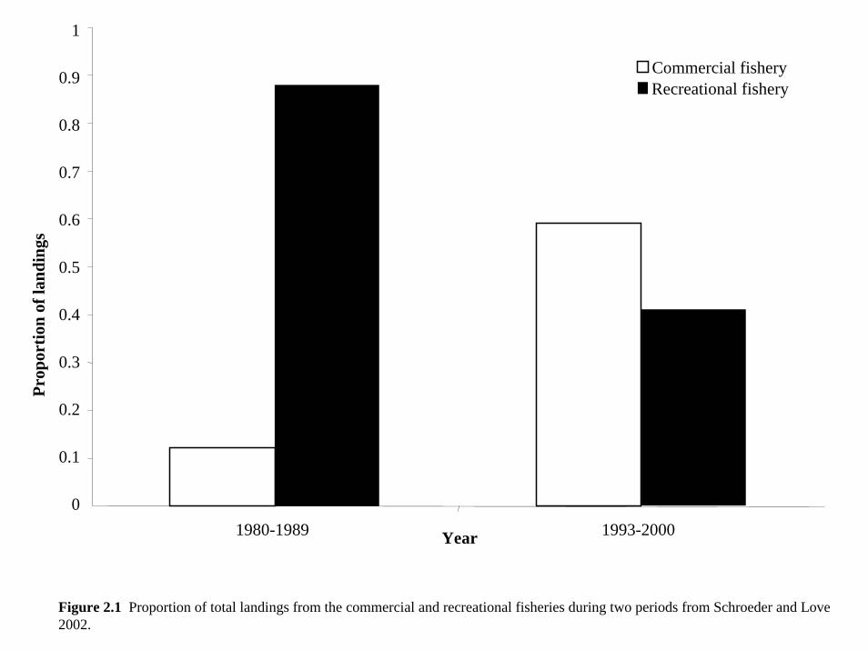
Commercial fisheryRecreational fishery

1980-1989 1993-20000

0.1

0.2

0.3

0.4

0.5

0.6

0.7

0.8

0.9

1

Year

Prop

ortio

n of

land

ings

Figure 2.1 Proportion of total landings from the commercial and recreational fisheries during two periods from Schroeder and Love 2002.

0

3

6

9

12

15

0 20 40 60 80

Fork length (cm)

Wei

ght (

kg)

W(L)=0.000027L2.857

Figure 3.1 The power relationship between length in cm and weight in kg (converted from DeMartini et al. 1994).

0

10

20

30

40

50

60

70

0 5 10 15 20

Age (years)

Fork

leng

th (c

m)

8

44

83 3

2

4322

1113

2528

Figure 3.2 Predicted size at age using the best-fit growth parameters compared with the observed mean size at age data from Warner (1975). Error bars show the 95% confidence interval around the mean size at age and sample sizes per age are also given.

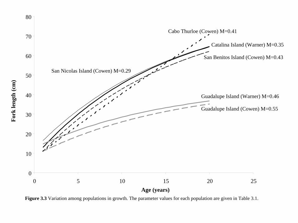
Catalina Island (Warner) M=0.35

Guadalupe Island (Warner) M=0.46

San Benitos Island (Cowen) M=0.43

Guadalupe Island (Cowen) M=0.55

Cabo Thurloe (Cowen) M=0.41

San Nicolas Island (Cowen) M=0.29

0

10

20

30

40

50

60

70

80

0 5 10 15 20 25Age (years)

Fork

leng

th (c

m)

Figure 3.3 Variation among populations in growth. The parameter values for each population are given in Table 3.1.

0

0.2

0.4

0.6

0.8

1

0 10 20 30 40 50 60Fork length (cm)

Prob

abili

ty o

f bei

ng m

atur

e an

d fe

mal

e

Catalina Island(Warner) M=0.35

Guadalupe Island(Warner) M=0.46

Guadalupe Island (Cowen) M=0.55

Cabo Thurloe(Cowen) M=0.41

San Benitos Island (Cowen) M=0.43

San Nicolas Island (Cowen) M=0.29

Figure 3.4 Variation among populations in maturity and sex change. Parameter values are given in Table 3.1.

0

500,000

1,000,000

1,500,000

2,000,000

0 0.5 1 1.5

Total body weight (kg)

Num

ber

of e

ggs o

r oo

cyte

s

Figure 3.5 The relationship between annual egg production or the estimated number of oocytes per female as a function of total body weight in kilograms. The dashed gray line shows the estimated total egg production of females as a function of their body weight (data for the estimate taken from DeMartini et al. 1994). We use this relationship in the baseline Synthesis model. The solid black line shows the number of oocytes per female as a function of female body weight (data for the estimate taken from Warner 1975 and the weight/length relationship published in DeMartini et al. 1994). We used this relationship in a sensitivity analysis.

0

200,000

400,000

600,000

800,000

1,000,000

1,200,000

1,400,000

0.5 1 1.5Weight (kg)

Ann

ual e

gg o

r oo

cyte

prod

uctio

n pe

r kg

bod

y w

eigh

t

.

Figure 3.6 Weight-specific egg production did not increase with individual body weight. The weight range shown is for the weights and lengths (15cm to 50 cm approximately) in which some individuals might be mature and female. The dashed gray line shows the expected number of eggs produced annually per kilogram of female body weight (data for the estimate taken from DeMartini et al. 1994). The solid black line shows the expected number of oocytes per kilogram of female body weight (data for the estimate takenfrom Warner 1975 and the weight/length relationship published in DeMartini et al. 1994). We used the data from DeMartini et al (1994) for the baseline model (slope=0 intercept=129,000) and the Warner derived slope and intercept (slope=55,000 and intercept=341,000) as a sensitivity analysis.

180

020406080

100120140160

1928

1932

1936

1940

1944

1948

1952

1956

1960

1964

1968

1972

1976

Year

Lan

ding

s (m

etri

c to

ns)

Mexico catch

No Mexico catch

0

20

40

60

80

100

120

140

160

1981

1983

1985

1987

1989

1991

1993

1995

1997

1999

2001

Lan

ding

s (m

etri

c to

ns)

PFEL

CFIS

PacFIN

CALCOM

Year

Figure 4.1b Comparing total Sheephead removals between two data sources; one including catch in Mexico (California’s Living Marine Resources - CLMR) and the other not including Mexico catch (PFEL). We used landings caught in Mexico and brought into California for total removals in our baseline model.

Figure 4.1a Comparing commercial landings (metric tons) by data source for overlapping time periods (1981-2002). No significant differences were detected (p=0.999).

catch

index

0

50

100

150

200

250

30019

61

1963

1965

1967

1969

1971

1973

1975

1977

1979

1981

1983

1985

1987

1989

1991

1993

1995

1997

1999

2001

2003

0

0.05

0.1

0.15

0.2

0.25

0.3

0.35

0.4

Year

Cat

ch (m

etri

c to

ns)

Spaw

ning

Inde

x

Figure 4.2 Comparing the annual variation (1961-2003) of landings (p<0.001) and the index of abundance (p=0.032) from CalCOFI larval surveys. Sheephead larvae appeared in the CalCOFI survey in 1961.

CPUE (Angler Day)CPUE (Angler)CPUE (converted to Angler)

0.00

0.01

0.02

0.03

0.04

0.05

0.06

0.0719

47

1949

1951

1953

1955

1957

1959

1961

1963

1965

1967

1969

1971

1973

1975

1977

1979

1981

CPU

E in

dex

YearFigure 4.3 Comparing units of catch per unit effort from 1947-1981from CPFV logbooks. Converting catch per angler day to make one series of catch per angler does not change the general trend in those years; however, there is a difference between thetwo indices (p=0.004). We used the separated time series of differing units in the baseline model; catch per angler day from 1947-1961 and catch per angler from 1960-1981.

Figure 4.4a The CPUE index from 1980-2003 was calculated using logbook block information. Once run through a GLM, we found that 70% of the cumulative block values were in the following five geographic regions: Northern Channel Islands, San Nicolas Island, Santa Catalina Island, San Clemente Island, and Tanner and Cortez Banks.

0

0.05

0.1

0.15

0.2

0.25

1980

1982

1984

1986

1988

1990

1992

1994

1996

1998

2000

2002

CPU

E in

dex

Year

0

0.02

0.04

0.06

0.08

0.1

0.12

0.14

JAN

FEB

MA

R

APR

MA

Y

JUN

JUL

AU

G

SEP

OC

T

NO

V

DEC

Chan IslandsSan Nicolas IslandCatalina IslandSan Clemente IslandBanks

(c)(b)

Chan IslandsSan Nicolas IslandCatalina IslandSan Clemente IslandBanks

Month

Figures 4.4 (b) shows the variability in the CPUE Index and (c) monthly effects for each Geographic Fishing Area. A separate glm was run for each area considering the interactions shown here.

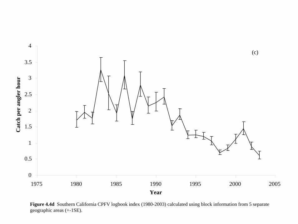
0

0.5

1

1.5

2

2.5

3

3.5

4

1975 1980 1985 1990 1995 2000 2005

Cat

ch p

er a

ngle

r ho

ur

Year

(c)

Figure 4.4d Southern California CPFV logbook index (1980-2003) calculated using block information from 5 separate geographic areas (+-1SE).

(a)

18 22 26 30 34 38 42 46 50 54 58 62 66 70 74 78

19931996199820002003

00.10.20.30.40.5

Percent Frequency

Fork length (cm)Year

1996199920012003

18 22 26 30 34 38 42 46 50 54 58 62 66 70 74 78

00.10.20.3

Percent Frequency

Fork length (cm)Year

(b)

Figures 4.5 shows length compositions for the commercial (a) hook-and-line and (b) trap fisheries.

(c)

19972001

00.10.20.3

PercentFrequency

Fork length (cm) Year

18 22 26 30 34 38 42 46 50 54 58 62 66 70 74 78

18 24 30 36 42 48 54 60 66 72 78197519771981198319851987198919941996199820002002

0

0.2

0.4

Percent Frequency

Fork length (cm)

Year

(d)

Figures 4.5 shows length compositions for the (c) setnet and (d) recreational fisheries.

30

32

34

36

38

40

42

44

46

1975 1977 1979 1981 1983 1985 1987 1989 1991 1993 1995 1997 1999 2001 2003Year

Fork

leng

th (c

m)

Figure 4.6 Average lengths of California Sheephead landed on CPFV’s, 1975-2003 (some years missing). Data for the 1975-1978 sample period are from Collins and Crooke, 1984-1989 sample period are from Ally et al, and all other years are from RecFIN (+- 1SE).

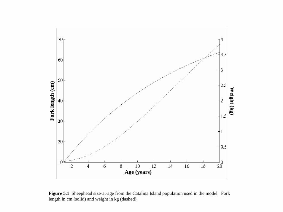
Age (years)

Fork

leng

th (c

m)

Weight (kg)

Figure 5.1 Sheephead size-at-age from the Catalina Island population used in the model. Forklength in cm (solid) and weight in kg (dashed).

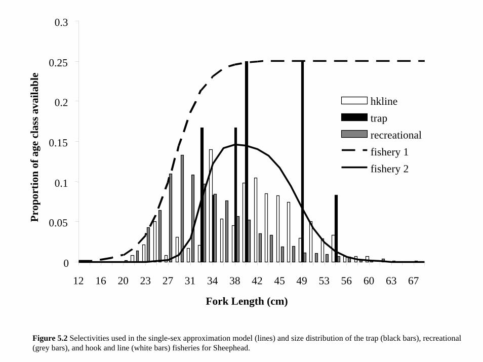
0

0.05

0.1

0.15

0.2

0.25

0.3

12 16 20 23 27 31 34 38 42 45 49 53 56 60 63 67

Fork Length (cm)

Prop

ortio

n of

age

cla

ss a

vaila

ble

hklinetraprecreationalfishery 1fishery 2

Figure 5.2 Selectivities used in the single-sex approximation model (lines) and size distribution of the trap (black bars), recreational (grey bars), and hook and line (white bars) fisheries for Sheephead.

0

0.1

0.2

0.3

0.4

0.5

0.6

0.7

0.8

0.9

1

12 15 17 19 21 23 25 27 30 32 34 36 38 40 42 45 47

Fork Length (cm)

Prop

ortio

n m

atur

e

Figure 5.3a Proportion of length class mature, regardless of sex. The bars show maturity data from Warner (1978), and the fitted line is calculated from Equation 5.6.

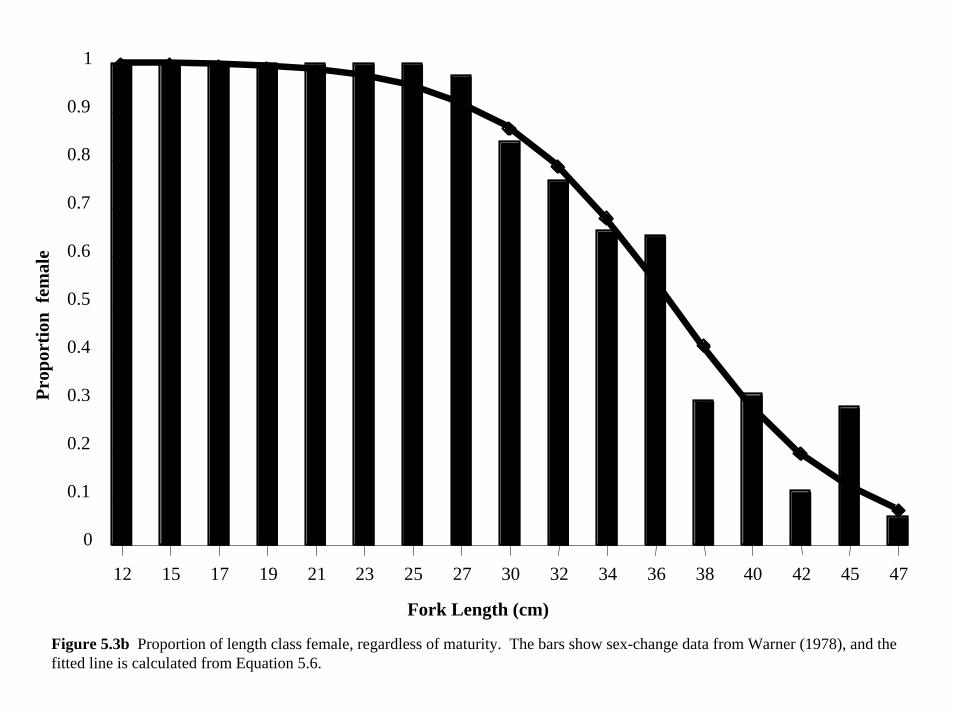
0

0.1

0.2

0.3

0.4

0.5

0.6

0.7

0.8

0.9

1

12 15 17 19 21 23 25 27 30 32 34 36 38 40 42 45 47

Fork Length (cm)

Prop

ortio

n fe

mal

e

Figure 5.3b Proportion of length class female, regardless of maturity. The bars show sex-change data from Warner (1978), and the fitted line is calculated from Equation 5.6.

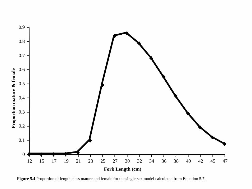
0

0.1

0.2

0.3

0.4

0.5

0.6

0.7

0.8

0.9

12 15 17 19 21 23 25 27 30 32 34 36 38 40 42 45 47Fork Length (cm)

Prop

ortio

n m

atur

e &

fem

ale

Figure 5.4 Proportion of length class mature and female for the single-sex model calculated from Equation 5.7.

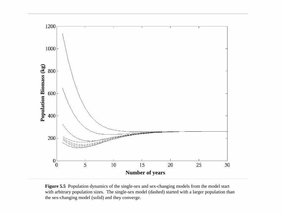
Number of years

Popu

latio

n B

iom

ass (

kg)

Figure 5.5 Population dynamics of the single-sex and sex-changing models from the model start with arbitrary population sizes. The single-sex model (dashed) started with a larger population than the sex-changing model (solid) and they converge.

smoothedEstimated inSynthesis

c) setnet

010203040

0 5 10 15 20 25 30 35 40

a) hook and line

048

121620

0 5 10 15 20 25 30

b) trap

01020304050

0 50 100 150 200 250 300

d) recreational

050

100150200

0 100 200 300 400 500 600 700 800

Actual sample size

Eff

ectiv

e sa

mpl

esi

ze

Figure 6.1 Effective sample sizes used in the Synthesis model.

0

0.1

0.2

0.3

0.4

0.5

0.6

0.7

0.8

0.9

1

10 20 30 40 50

recreational

setnet

trap

hook and line

Sele

ctiv

ity

Length (cm)

Figure 6.2 The selectivities for each of the four fisheries in the best-fit Synthesis model.

010002000300040005000600070008000

1947

1950

1953

1956

1959

1962

1965

1968

1971

1974

1977

1980

1983

1986

1989

1992

1995

1998

2001

Year

Beg

inni

ng b

iom

ass

(met

ric

tons

)

SRR

010002000300040005000600070008000

0 20000 40000 60000 80000Spawning biomass (t)

Rec

ruitm

ent (

t+1)

Recruitment

Biomass

Year

Beg

inni

ng b

iom

ass

(met

ric

tons

)

0500

1000150020002500300035004000

1947

1950

1953

1956

1959

1962

1965

1968

1971

1974

1977

1980

1983

1986

1989

1992

1995

1998

2001

0100002000030000400005000060000700008000090000

BEG BIOEGG PROD.

Egg productiona)

b)

c)

Figure 6.3 (a) The historical total biomass and female spawning biomass (b) recruitment, and (c) the relationship between recruitment and spawning biomass estimated by the baseline Synthesis model.

CPFV logbooks CPUE 1960-1981

00.010.020.030.040.050.060.070.080.090.1

1960

1962

1964

1966

1968

1970

1972

1974

1976

1978

1980

CPU

E (c

atch

per

ang

ler)

CPU

E (c

atch

per

ang

ler

day)

00.01

0.020.03

0.040.05

0.06

0.07

0.08

1947

1949

1951

1953

1955

1957

1959

1961

CPFV logbooks CPUE 1947-1961

CPFV logbooks CPUE 1980-2003

0

0.050.1

0.150.2

0.25

0.3

0.35

0.4

1951

1955

1959

1963

1967

1971

1975

1979

1983

1987

1991

1995

1999

2003

Lar

val a

bund

ance

inde

x

CalCOFI larval survey 1951-2003

CPU

E (c

atch

per

ang

ler

hour

)

0

0.5

1

1.5

2

2.5

3

3.5

1980

1982

1984

1986

1988

1990

1992

1994

1996

1998

2000

2002

YearFigure 6.4 The estimated (solid line) and observed (black squares) abundance indices for the baseline Synthesis model.

0

0.1

0.2

0.3

0.4

0.5

0.6

0.7

0.8

0.9

1

Rec

ruit(

t)/S

SB(t

-1)

1948

1950

1952

1954

1956

1958

1960

1962

1964

1966

1968

1970

1972

1974

1976

1978

1980

1982

1984

1986

1988

1990

1992

1994

1996

1998

2000

2002

Year

Figure 6.5 Recruit per spawning biomass was estimated to be variable through time in the baseline Synthesis model.

0

50

100

150

200

250

1940 1950 1960 1970 1980 1990 2000 2010

Lan

ding

s (m

etri

c to

ns)

Figure 6.6 Landings for the hook and line commercial fishery in the Synthesis model.

0

50

100

150

200

250

1975 1980 1985 1990 1995 2000 2005

Lan

ding

s (m

etri

c to

ns)

Figure 6.7 Landings for the trap commercial fishery in the Synthesis model.

0

50

100

150

200

250

1975 1980 1985 1990 1995 2000 2005

Lan

ding

s (m

etri

c to

ns)

Figure 6.8 Landings for the setnet commercial fishery in the Synthesis model.

0

50

100

150

200

250

1940 1950 1960 1970 1980 1990 2000 2010

Lan

ding

s (m

etri

c to

ns)

Figure 6.9 Landings for the recreational fishery in the Synthesis model.

0 10 20 30 40 50 60

Hook and Line

Length (cm)

Yea

r

199019921994199619982000200220042006

715131012

8152712

Setnet

Length (cm)

Yea

r

1996199719981999200020012002

0 10 20 30 40 50 60

38

12

8

Recreational Trap

Length (cm)

Yea

r1995199619971998199920002001200220032004

0 10 20 30 40 50 60

2211712854168

248301970

1975198019851990199520002005

0 10 20 30 40 50 60Length (cm)

Yea

r

Figure 6.10 Bubble plots representing the fit between the observed and estimated length compositions for the baseline Synthesis model. The area of the circle indicates the deviation between the observed and estimated values. Filled circles represent a positive deviation and empty circles represent a negative deviation. Sample sizes are also given for the commercial fisheries.

0

0.02

0.04

0.06

0.08

0.1

0.12

0.14

0.16

0.18

1940 1950 1960 1970 1980 1990 2000 2010Year

Exp

loita

tion

rate

Figure 6.11 Historical exploitation rate of Sheephead as estimated by the baseline Synthesis model.

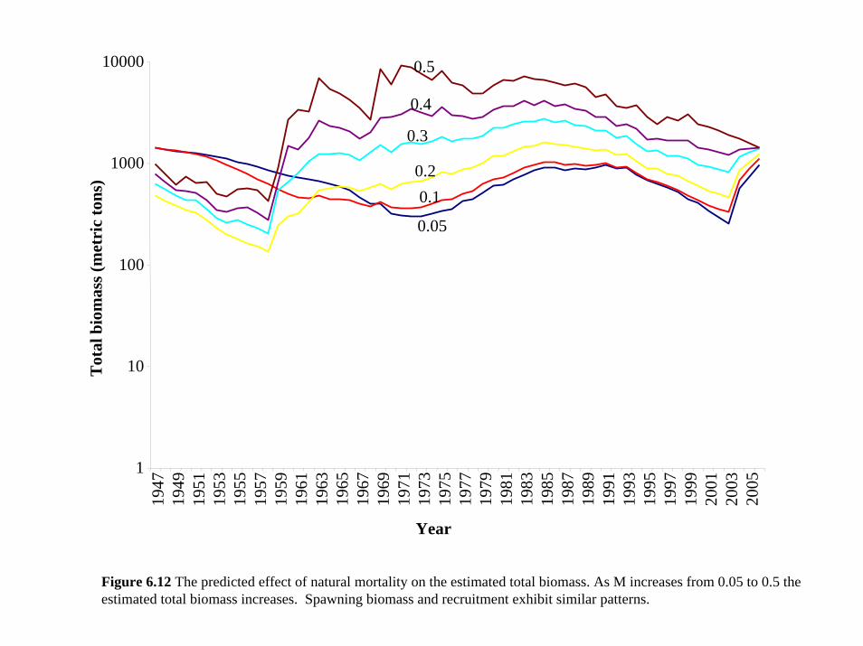
Year

Tot

al b

iom

ass (

met

ric

tons

)

1

10

100

1000

10000

1947

1949

1951

1953

1955

1957

1959

1961

1963

1965

1967

1969

1971

1973

1975

1977

1979

1981

1983

1985

1987

1989

1991

1993

1995

1997

1999

2001

2003

2005

0.05

0.10.2

0.3

0.4

0.5

Figure 6.12 The predicted effect of natural mortality on the estimated total biomass. As M increases from 0.05 to 0.5 the estimated total biomass increases. Spawning biomass and recruitment exhibit similar patterns.

300

320

340

360

380

400

420

0.05 0.1 0.2 0.3 0.4 0.5

-Log

like

lihoo

d

342

343

344

345

346

0.3 0.4 0.5

Mortality

Figure 6.13 The total (negative) log-likelihood of the model for a sensitivity analyses of natural mortality rate as mortality varies from 0.05 to 0.5.

1

10

100

1000

10000

1947

1950

1953

1956

1959

1962

1965

1968

1971

1974

1977

1980

1983

1986

1989

1992

1995

1998

2001

2004

Year

Tot

al b

iom

ass (

met

ric

tons

)

0.1

0.150.2

0.25

0.29

Figure 6.14 The effect of the coefficient of variation in growth (CV1 and CV2) on the estimated total biomass. As CV1 and CV2 increase from 0.10 to 0.29, the estimated total biomass decreases. Spawning biomass exhibits a similar pattern.

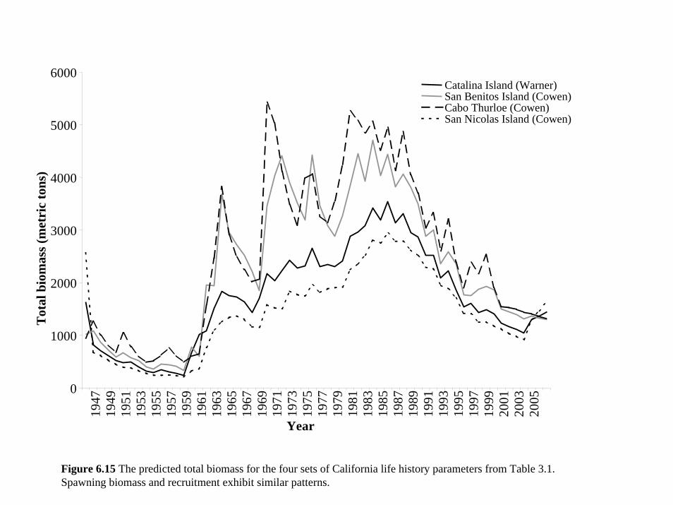
0

1000

2000

3000

4000

5000

6000

1947

1949

1951

1953

1955

1957

1959

1961

1963

1965

1967

1969

1971

1973

1975

1977

1979

1981

1983

1985

1987

1989

1991

1993

1995

1997

1999

2001

2003

2005

Year

Tot

al b

iom

ass (

met

ric

tons

)

Catalina Island (Warner)San Benitos Island (Cowen)Cabo Thurloe (Cowen)San Nicolas Island (Cowen)

Figure 6.15 The predicted total biomass for the four sets of California life history parameters from Table 3.1. Spawning biomass and recruitment exhibit similar patterns.

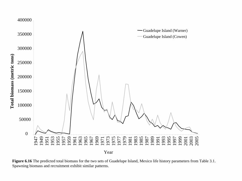
Year

Tot

al b

iom

ass (

met

ric

tons

)

0

50000

100000

150000

200000

250000

300000

350000

400000

1947

1949

1951

1953

1955

1957

1959

1961

1963

1965

1967

1969

1971

1973

1975

1977

1979

1981

1983

1985

1987

1989

1991

1993

1995

1997

1999

2001

2003

2005

Guadelupe Island (Warner)Guadelupe Island (Cowen)

Figure 6.16 The predicted total biomass for the two sets of Guadelupe Island, Mexico life history parameters from Table 3.1. Spawning biomass and recruitment exhibit similar patterns.

0

100

200

300

400

500

600

700

800Catalina

Island(Warner)

GuadelupeIsland

(Warner)

San BenitosIsland

(Cowen)

GuadelupeIsland

(Cowen)Cabo Thurloe

(Cowen)

San NicolasIsland

(Cowen)

-log

like

lihoo

d

Figure 6.17 The negative log likelihood of the model as the life history parameters are varied. The Guadelupe parameters do not lead to a good fit with the data while the parameters from the four California populations fit the data similarly. The parameters used for the baseline model were based on the Catalina data from Warner (1975) which lead to the best fit between the data and the model.

0

1000

2000

3000

4000

5000

6000

7000

800019

4719

4919

5119

5319

5519

5719

5919

6119

6319

6519

6719

6919

7119

7319

7519

7719

7919

8119

8319

8519

8719

8919

9119

9319

9519

9719

9920

0120

0320

05

Year

Rec

ruits

00.10.51

Figure 6.18 The effect of increasing the likelihood weights on the stock recruitment curve from zero to one on the estimated recruitment in the model. The freely estimated values (zero weight on the curve), show greater temporal variation but a similar trend to the other values.

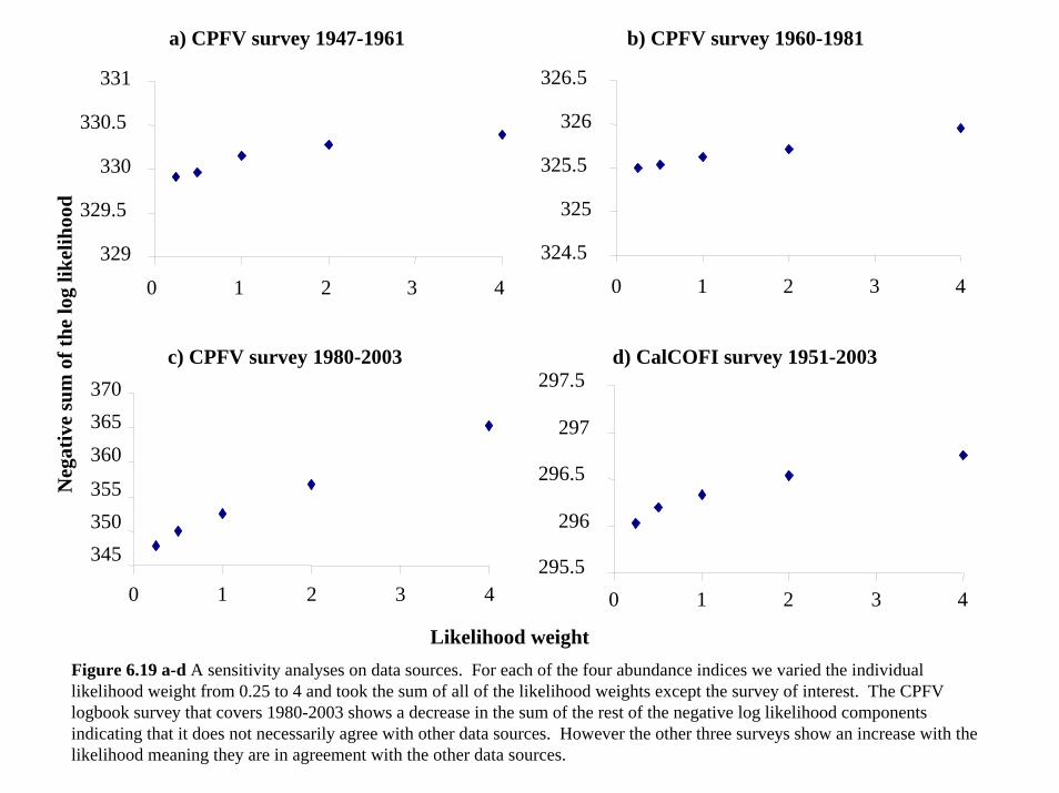
Neg

ativ

e su

m o

f the

log

likel

ihoo

d

Likelihood weight

a) CPFV survey 1947-1961

329

329.5

330

330.5

331

0 1 2 3 4

b) CPFV survey 1960-1981

324.5

325

325.5

326

326.5

0 1 2 3 4

d) CalCOFI survey 1951-2003

295.5

296

296.5

297

297.5

0 1 2 3 4

c) CPFV survey 1980-2003

345350355

360365370

0 1 2 3 4

Figure 6.19 a-d A sensitivity analyses on data sources. For each of the four abundance indices we varied the individual likelihood weight from 0.25 to 4 and took the sum of all of the likelihood weights except the survey of interest. The CPFV logbook survey that covers 1980-2003 shows a decrease in the sum of the rest of the negative log likelihood components indicating that it does not necessarily agree with other data sources. However the other three surveys show an increase with the likelihood meaning they are in agreement with the other data sources.

Neg

ativ

e su

m o

f the

log

likel

ihoo

d a) Hook and line

300305

310315320

325330

0 1 2 3 4c) setnet

320325330335340345350

0 1 2 3 4

b) trap

290295300305310315320

0 1 2 3 4d) recreational length compositions

140145150155

160165170

0 1 2 3 4

Likelihood weight

Figure 6.20 a-d A sensitivity analyses on data sources. For each set of length compositions associated with one of the four fisheries, we varied the individual likelihood weight from 0.25 to 4 and took the sum of all of the likelihood components exceptthe length composition being varied. They all tend to increase with the likelihood weight indicating that they tend to be in agreement with the other data sources.

Likelihood weight

Neg

ativ

e su

m o

f the

log

likel

ihoo

d

a) All four surveys

270

275

280

285

290

0 1 2 3 4

b) All length compositions

60

65

70

75

80

0 1 2 3 4

Figure 6.21 Sensitivity analysis on data sources. We give the total log-likelihood of the model when we (a) varied the likelihood weight of all four surveys simultaneously while keeping all other likelihood weights constant (and equal to 1.0) and (b) varied the likelihood weight of all four sets of length compositions while keeping all other likelihood weights constant.

Figure 6.22 a-d We varied the likelihood weight of each of the four surveys individually while holding all other likelihood weights at the baseline level at one. In each panel, the likelihood component of one survey is shown as another survey’s likelihood weight is varied. We focus on comparing the CPFV surveys with the CalCOFI survey.

46

46.1

46.2

46.3

46.4

46.5

46.6

0 1 2 3 4

a) CPFV 1947-1961 and CalCOFI Survey-L

og li

kelih

ood

com

pone

nt

b) CPFV 1960-1981 and CalCOFI Survey

46.15

46.2

46.25

46.3

46.35

46.4

0 1 2 3 4

c) CPFV 1980-2003 and CalCOFI Survey

46.2146.2246.2346.2446.2546.2646.2746.28

0 1 2 3 4

d) CalCOFI Survey and CPFV 1947-1961

12.2

12.3

12.4

12.5

12.6

12.7

0 1 2 3 4

Likelihood weight

e) CalCOFI Survey and CPFV 1960-1981

16.85

16.9

16.95

17

17.05

0 1 2 3 4

Likelihood weight

-Log

like

lihoo

d co

mpo

nent

f) CalCOFI Survey and CPFV 1980-2003

10

10.05

10.1

10.15

10.2

0 1 2 3 4

Figure 6.22 e-f Continued. We varied the likelihood weight of each of the four surveys individually while holding all other likelihood weights at the baseline level of one. In each panel, the likelihood component of one survey is shown as another survey’s likelihood weight is varied. We focus on comparing the CPFV surveys with the CalCOFI survey.

a) Varying the emphasis on the hook & line length compositions

31.631.8

3232.232.432.632.8

3333.2

0 1 2 3 4

trapsetnetrecreational

b) Varying the emphasis on the trap length compositions

383940414243444546

0 1 2 3 4

hook and linesetnetrecreational

c) Varying the emphasis on the setnet length compositions

Likelihood weight of composition

-log

likel

ihoo

d co

mpo

nent

12.4

12.6

12.8

13

13.2

13.4

13.6

13.8

0 1 2 3 4

hook and linetraprecreational

d) Varying the emphasis on recreational length compositions

186188190192194196198200202

0 1 2 3 4

hook and linetrapsetnet

Figure 6.23 a-d Sensitivity analyses on data sources. We varied the individual likelihood weights of each length composition whileholding all other likelihood weights at the baseline level of one. Each panel represents the change in the individual likelihood componentof the three length compositions while the weight of the fourth set of length compositions is varied.

0

0.01

0.02

0.03

0.04

0.05

0.06

0.07

0.08

0.09

0.10

1947

1950

1953

1956

1959

1962

1965

1968

1971

1974

1977

1980

Year

CPU

E (c

atch

per

ang

ler)

Figure 6.24 Sensitivity analysis on the fit to the combined CPFV (1947-1981) survey. Black squares are the observed values and the solid line is the estimated abundance index.

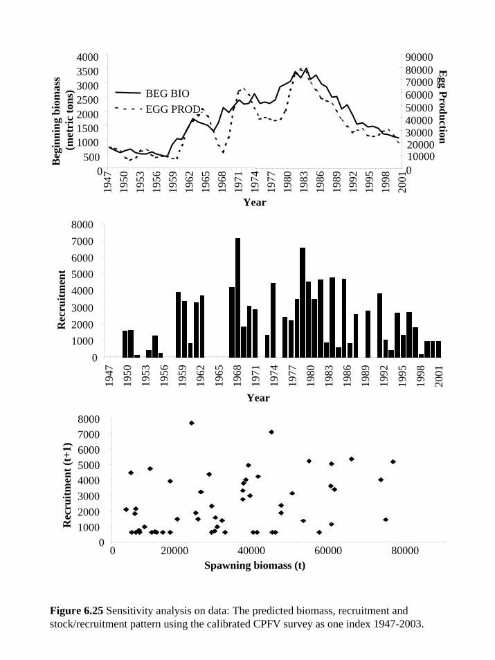
Year

Beg

inni

ng b

iom

ass

(met

ric

tons

)

1947

1950

1953

1956

1959

1962

1965

1968

1971

1974

1977

1980

1983

1986

1989

1992

1995

1998

2001

0500

1000150020002500300035004000

0100002000030000400005000060000700008000090000

BEG BIOEGG PROD.

010002000300040005000600070008000

1947

1950

1953

1956

1959

1962

1965

1968

1971

1974

1977

1980

1983

1986

1989

1992

1995

1998

2001

Year

Rec

ruitm

ent

Spawning biomass (t)

Rec

ruitm

ent (

t+1)

010002000300040005000600070008000

0 20000 40000 60000 80000

Figure 6.25 Sensitivity analysis on data: The predicted biomass, recruitment and stock/recruitment pattern using the calibrated CPFV survey as one index 1947-2003.

Egg Production

Exploitation (catch/total biomass)

Spaw

ning

pot

entia

l rat

io

0

0.2

0.4

0.6

0.8

1

0 0.05 0.1 0.15 0.2

target SPR

estimatedcurrent exploitation

total

female

male (7+)

male (8+)

mature (4+)

Figure 7.1 Estimated status of the stock as predicted by the baseline model. We give the relative spawning potential ratio (SPR) for female, mature (age 4 and above), male (age 7 and above or age 8 and above) and total biomass. Current exploitation is shown with the dashed vertical line. Female spawning potential ratio is estimated to be reduced to 80% of unfished levels while relative male spawning potential ratio is estimated to be reduced by about 65%. Equilibrium calculations are based on current (2003) fishing mortality associated with each fishery.

Exploitation

Spaw

ning

pot

entia

l rat

ioM=0.2 max age=20M=0.07 max age=53

current

0

0.1

0.2

0.3

0.4

0.5

0.6

0.7

0.8

0.9

1

0 0.1 0.2 0.3 0.4 0.5

target

current

target

0

0.1

0.2

0.3

0.4

0.5

0.6

0.7

0.8

0.9

1

0 0.1 0.2 0.3 0.4 0.5

Figure 7.2 Natural mortality affects the estimated status of the stock. We give the relative spawning potential ratio (SPR) for female (thick grey line), male (age 7 and above, thin grey line) and total biomass (black line) for two additional natural mortality values. Natural mortality was estimated using Hoenig (1983) and the observed maximum age of Sheephead from two different sources. For further details see the text. Current estimated exploitation differs between the models as natural mortality changes because the estimated total and spawning biomass are affected by natural mortality. Equilibrium calculations are based on current (2003) fishing mortality associated with each fishery.

0

0.2

0.4

0.6

0.8

1 total SPR

male SPR

female SPR

CatalinaIsland

(Warner)

San BenitosIsland

(Cowen)

CaboThurloe(Cowen)

San NicolasIsland

(Cowen)

Spaw

ning

pot

entia

l rat

io

Figure 7.3 The estimated current status of the stock is also affected by the combination of life history parameters used. We ran the model with each of the six sets of parameters given in Table 3.1 and calculated the estimated relative spawning potential ratios (total, female and male) for each model, this figure shows only the four nearshore populations. Equilibrium calculations are based on current (2003) fishing mortality associated with each fishery.

Figure 7.4 Variable recruitment leads to temporal variation in expected total and spawning biomass even in the absence of fishing mortality. The results presented here are based on a single projection showing for total (black line) and female (grey line) spawning biomass in the absence of fishing assuming that recruitment is selected randomly from model estimated recruitment from 1970-1995.

2000 2020 2040 2060 2080 2100Year

Bio

mas

s (m

etri

c to

ns)

0

500

1000

1500

2000

2500

3000

3500

4000

4500

5000

0

10000

20000

30000

40000

50000

60000

70000

80000

90000

100000

Spaw

ning

bio

mas

s (eg

g x

105 )

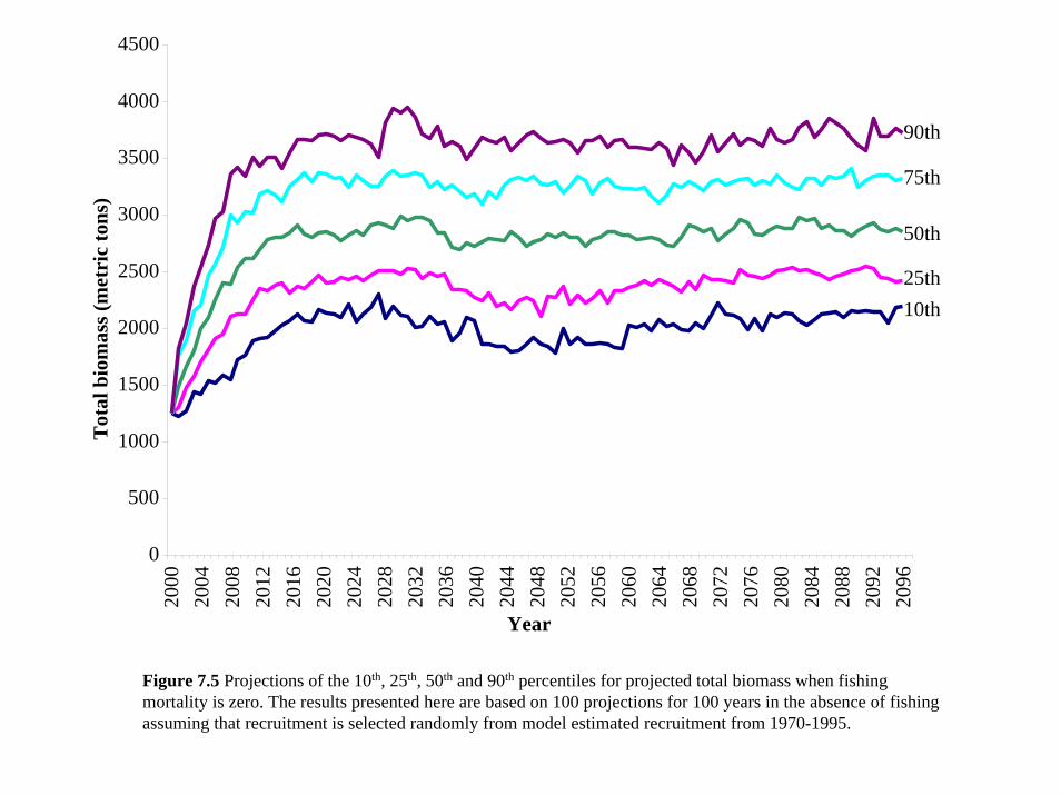
Year

Tot

al b

iom

ass (

met

ric

tons

)

0

500

1000

1500

2000

2500

3000

3500

4000

4500

2000

2004

2008

2012

2016

2020

2024

2028

2032

2036

2040

2044

2048

2052

2056

2060

2064

2068

2072

2076

2080

2084

2088

2092

2096

10th25th

50th

75th

90th

Figure 7.5 Projections of the 10th, 25th, 50th and 90th percentiles for projected total biomass when fishing mortality is zero. The results presented here are based on 100 projections for 100 years in the absence of fishing assuming that recruitment is selected randomly from model estimated recruitment from 1970-1995.

Year

Spaw

ning

bio

mas

s (eg

gs x

105 )

0

10,000

20,000

30,000

40,000

50,000

60,000

70,000

80,000

90,000

2000

2004

2008

2012

2016

2020

2024

2028

2032

2036

2040

2044

2048

2052

2056

2060

2064

2068

2072

2076

2080

2084

2088

2092

2096

10th

25th

50th

75th

90th

Figure 7.6 Projections of the 10th, 25th, 50th and 90th percentiles for projected spawning biomass when fishing mortality is zero. The results presented here are based on 100 projections for 100 years in the absence of fishing assuming that recruitment is selected randomly from model estimated recruitment from 1970-1995.

Total biomass (metric tons)

Freq

uenc

y

0

50

100

150

200

250

0 1000 2000 3000 4000 5000 6000

F=0

F=0.2

F=0.5

Figure 7.7 Frequency distributions of projected total biomass in the future (of the baseline model) when future fishing mortality is fixed at 0, 0.2 and 0.5. The distribution of total biomass is based on projections over 50 years after having allowed the projections to stabilize. The results presented here are based on 100 projections for 100 years assuming that recruitment is selected randomly from model estimated recruitment from 1970-1995.

Total biomass (metric tons)

Freq

uenc

y

M=0.35 (baseline)

0

50

100

150

200

250

0 1000 2000 3000 4000 5000 6000 7000 8000 9000

M=0.2

Figure 7.8 Frequency distributions of projected total biomass in the future (of the baseline model) when fishing mortality is zero (F=0) and natural mortality is 0.35 (baseline case) and 0.2. The distribution of total biomass is based on projections over 50 years after having allowed the projections to stabilize. The results presented here are based on 100 projections for 100 years assuming that recruitment is selected randomly from model estimated recruitment from 1970-1995.

Total biomass (metric tons)

Freq

uenc

y

0

50

100

150

200

250

0 1000 2000 3000 4000 5000 6000 7000 8000 9000

CV fit by the model (baseline)

CV=0.1

CV=0.2

CV=0.3

Figure 7.9 Frequency distributions of projected total biomass in the future (of the baseline model) when fishing mortality is zero and the coefficient of variation is estimated by the model (baseline case), 0.1, 0.2 and 0.3. The distribution of total biomass is based on projections over 50 years after having allowed the projections to stabilize. The results presented here are based on 100 projections for 100 years assuming that recruitment is selected randomly from model estimated recruitment from 1970-1995.

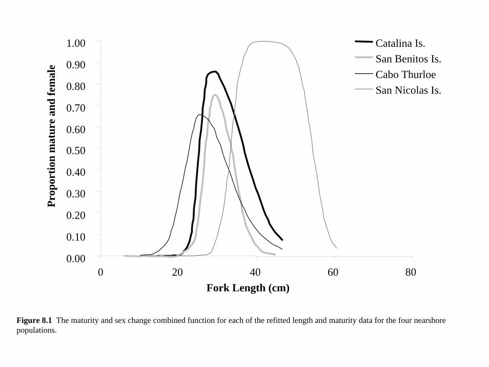
0.00

0.10

0.20

0.30

0.40

0.50

0.60

0.70

0.80

0.90

1.00

0 20 40 60 80Fork Length (cm)

Prop

ortio

n m

atur

e an

d fe

mal

eCatalina Is.San Benitos Is.Cabo ThurloeSan Nicolas Is.

Figure 8.1 The maturity and sex change combined function for each of the refitted length and maturity data for the four nearshore populations.

Length (cm, lower edge of bin)

Sele

ctiv

ity

00.10.20.30.40.50.60.70.80.9

1

10 20 30 40 50 60 70 80

HKLINE

TRAPS

SETNET

RECREATIONAL

Figure 8.2 Estimated selectivities for each of the four fisheries in the final Synthesis model. Results are shown for the case where M=0.2. However, alternative natural mortality values (M=0.15 and M=0.3) lead to the same pattern.

Figure 8.3 (a) The historical total biomass and spawning biomass (b) recruitment, and (c) the relationship between recruitment and spawning output estimated by the final Synthesis model when M=0.2. The round markers indicate recruitment between 1993-2000.

1947

1952

1957

1962

1967

1972

1977

1982

1987

1992

1997

2002

0

500

1000

1500

2000

Year

Rec

ruitm

ent

Year

Beg

inni

ng b

iom

ass

(met

ric

tons

)1000

1500

2000

1947

1952

1957

1962

1967

1972

1977

1982

1987

1992

1997

2002

10000

20000

30000

40000

50000

0

500

0

Total Biomass

Eggs

Egg production

(c)

0200400600800

10001200140016001800

0 10000 20000 30000 40000 50000Female egg production (t)

Rec

ruitm

ent (

t+1)

(b)

(a)

Figure 8.4 (a) The historical total biomass and spawning biomass (b) recruitment, and (c) the relationship between recruitment and spawning output estimated by the final Synthesis model when M=0.15the round markers indicate recruitment between 1993-2000.

0

200

400

600

800

1000

1200

1947

1950

1953

1956

1959

1962

1965

1968

1971

1974

1977

1980

1983

1986

1989

1992

1995

1998

2001

Year

Rec

ruitm

ent

Year

1947

1950

1953

1956

1959

1962

1965

1968

1971

1974

1977

1980

1983

1986

1989

1992

1995

1998

2001

Beg

inni

ng b

iom

ass

(met

ric

tons

)

0

2000

4000

6000

8000

10000

0 20000 40000 60000 80000

Female egg production (t)

Rec

ruitm

ent (

t+1)

0200400600800

10001200140016001800

05000100001500020000250003000035000

Total biomass

Eggs

Egg production

(b)

(c)

(a)

Figure 8.5 (a) The historical total biomass and spawning biomass (b) recruitment, and (c) the relationship between recruitment and spawning output estimated by the final Synthesis model when M=0.3 the round markers indicate recruitment between 1993-2000.

Year

1947

1952

1957

1962

1967

1972

1977

1982

1987

1992

1997

2002

0500

100015002000250030003500

Beg

inni

ng b

iom

ass

(met

ric

tons

)

01000020000300004000050000600007000080000Tot. Biomass

Eggs

0

2000

4000

6000

8000

10000

1947

1952

1957

1962

1967

1972

1977

1982

1987

1992

1997

2002

Year

Rec

ruitm

ent

(a)

(b)

(c)

Egg production

0

200

400

600

800

1000

1200

0 10000 20000 30000 40000Female egg production (t)

Rec

ruitm

ent (

t+1)

Year

00.010.020.030.040.050.060.070.08

1947

1949

1951

1953

1955

1957

1959

1961

CPFV1 CPUE

0

0.02

0.04

0.06

0.08

0.1

1960

1963

1966

1969

1972

1975

1978

1981

CPFV2 CPUE

00.5

11.5

22.5

33.5

1980

1983

1986

1989

1992

1995

1998

2001

CPFV3 CPUE

00.05

0.10.15

0.20.25

0.30.35

0.4

1951

1958

1965

1972

1979

1986

1993

2000

CalCOFI Survey

Inde

x of

abu

ndan

ce

Figure 8.6 The estimated (solid line) and observed (black squares) abundance indices for the final Synthesis model when M=0.2.

00.010.020.030.040.050.060.070.08

1947

1949

1951

1953

1955

1957

1959

1961

CPFV1 CPUE

00.5

11.5

22.5

33.5

1980

1982

1984

1986

1988

1990

1992

1994

1996

1998

2000

2002

CPFV3 CPUE

00.010.020.030.040.050.060.070.080.09

0.1

1960

1962

1964

1966

1968

1970

1972

1974

1976

1978

1980

CPFV2 CPUE

00.05

0.10.15

0.20.25

0.30.35

0.4

1951

1955

1959

1963

1967

1971

1975

1979

1983

1987

1991

1995

1999

2003

CalCOFI Survey

Inde

x of

abu

ndan

ce

YearFigure 8.7 The estimated (solid line) and observed (black squares) abundance indices for the final Synthesis model when M=0.15.

Year

00.010.020.030.040.050.060.070.08

1947

1949

1951

1953

1955

1957

1959

1961

CPFV1 CPUE

00.5

11.5

22.5

33.5

1980

1983

1986

1989

1992

1995

1998

2001

CPFV3 CPUE

0

0.02

0.04

0.06

0.08

0.1

1960

1963

1966

1969

1972

1975

1978

1981

CPFV2 CPUE

00.05

0.10.15

0.20.25

0.30.35

0.4

1951

1958

1965

1972

1979

1986

1993

2000

CalCOFI Survey

Inde

x of

abu

ndan

ce

Figure 8.8 The estimated (solid line) and observed (black squares) abundance indices for the final Synthesis model when M=0.3.

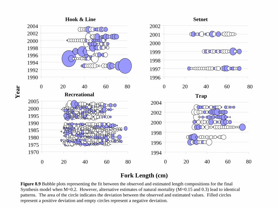
Yea

rHook & Line

19901992199419961998200020022004

0 20 40 60 80Recreational

19701975198019851990199520002005

0 20 40 60 80

Fork Length (cm)

Setnet

1996199719981999200020012002

0 20 40 60 80

Trap

1994

1996

1998

2000

2002

2004

0 20 40 60 80

Figure 8.9 Bubble plots representing the fit between the observed and estimated length compositions for the final Synthesis model when M=0.2. However, alternative estimates of natural mortality (M=0.15 and 0.3) lead to identical patterns. The area of the circle indicates the deviation between the observed and estimated values. Filled circles represent a positive deviation and empty circles represent a negative deviation.

Figure 8.10 Exploitation rate of Sheephead as estimated by the final Synthesis model when M=0.20 (a), M=0.15 (b), and M=0.30 (c).

Exp

loita

tion

Rat

e

00.020.040.060.08

0.10.120.140.16

1940 1950 1960 1970 1980 1990 2000 2010Year

(c)

0

0.05

0.1

0.15

0.2

0.25

0.3

1940 1950 1960 1970 1980 1990 2000 2010

(a)

0

0.05

0.1

0.15

0.2

0.25

0.3

0.35

1940 1950 1960 1970 1980 1990 2000 2010

(b)

Figure 8.11 Relative spawning potential ratio (SPR) for female (upper curve), mature (middle curve), and male (lower curve) biomass based on the final model when M=0.2 (a), M=0.15 (b), and M=0.30 (c). Current exploitations are shown with the vertical thin black line, target exploitations are shown with the vertical solid grey line, and target levels are shown by the horizontal grey line.

(a)

(c)

Exploitation (catch/total biomass)

Rel

ativ

e SP

R

(b)

0

0.2

0.4

0.6

0.8

1

0 0.05 0.1 0.15 0.2 0.25 0.3 0.35

0

0.2

0.4

0.6

0.8

1

0 0.1 0.2 0.3 0.4 0.5

0

0.2

0.4

0.6

0.8

1

0 0.1 0.2 0.3 0.4

Figure 8.12 Projections of the 25th, 50th and 75th percentiles for projected total biomass when fishing mortality is zero for M=0.20 (a), M=0.15 (b), and M=0.30 (c). The results presented here are based on 100 projections for 100 years in the absence of fishing assuming that recruitment is selected randomly from model estimated recruitment from 1970-1995.

0

500

1000

1500

2000

2500

3000

3500

1980 2000 2020 2040 2060 2080 2100 2120

0500

1000150020002500300035004000

1980 2000 2020 2040 2060 2080 2100 2120

Tot

al b

iom

ass (

met

ric

tons

)

Year

(a)

0500

1000150020002500300035004000

1980 2000 2020 2040 2060 2080 2100 2120

(c)

(b)25%50%75%

25%50%75%

25%50%75%

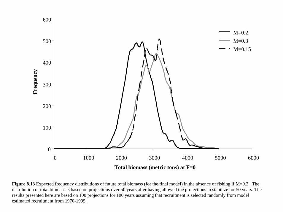
0

100

200

300

400

500

600

0 1000 2000 3000 4000 5000 6000

Total biomass (metric tons) at F=0

Freq

uenc

yM=0.2M=0.3M=0.15

Figure 8.13 Expected frequency distributions of future total biomass (for the final model) in the absence of fishing if M=0.2. The distribution of total biomass is based on projections over 50 years after having allowed the projections to stabilize for 50 years. The results presented here are based on 100 projections for 100 years assuming that recruitment is selected randomly from model estimated recruitment from 1970-1995.

0

100

200

300

400

500

600

700

800

900

1000

0 500 1000 1500 2000 2500 3000 3500 4000

Total biomass (metric tons) at F=Fspr

Freq

uenc

y

M=0.2M=0.3M=0.15

Figure 8.14 Expected frequency distributions of future total biomass (for the final model) when future fishing mortality adopts the 60/20 plan outlined by the NFMP and is set at the target level which allows the spawning potential ratio based on mature biomass to be reduced to 50% of the estimated unfished situation (CDFG 2002). The distribution of total biomass is based on projections over 50 years after having allowed the projections to stabilize for 50 years. The results presented here are based on 100 projections for 100 years assuming that recruitment is selected randomly from model estimated recruitment from 1970-1995.

0

50

100

150

200

250

2004

2006

2008

2010

2012

2014

2016

2018

2020

2022

2024

2026

2028

10th25th50th75th90th

0

20

40

60

80

100

120

140

160

180

2004

2006

2008

2010

2012

2014

2016

2018

2020

2022

2024

2026

2028

Year

Tot

al y

ield

(met

ric

tons

)

10th25th50th75th90th

(a)

(b)

Figure 8.15 Allowable catch under NFMP 60/20 policy (CDFG 2002) for California Sheephead for the final model when M=0.2 for females only (a) and the total mature population (b). Projection assumptions are the same as described in Figure 8.13.

Tot

al b

iom

ass (

met

ric

tons

)

0

500

1000

1500

2000

2500

3000

3500

4000

2004

2006

2008

2010

2012

2014

2016

2018

2020

2022

2024

2026

2028

10th25th50th75th90th

0

500

1000

1500

2000

2500

3000

3500

4000

2004

2006

2008

2010

2012

2014

2016

2018

2020

2022

2024

2026

2028

Year

10th25th50th75th90th

(a)

(b)

Figure 8.16 Projected population bioamass under NFMP 60/20 policy (CDFG 2002) for California Sheephead for the final model when M=0.2 for females only (a) and the total mature population (b). Projection assumptions are the same as described in Figure 8.13.

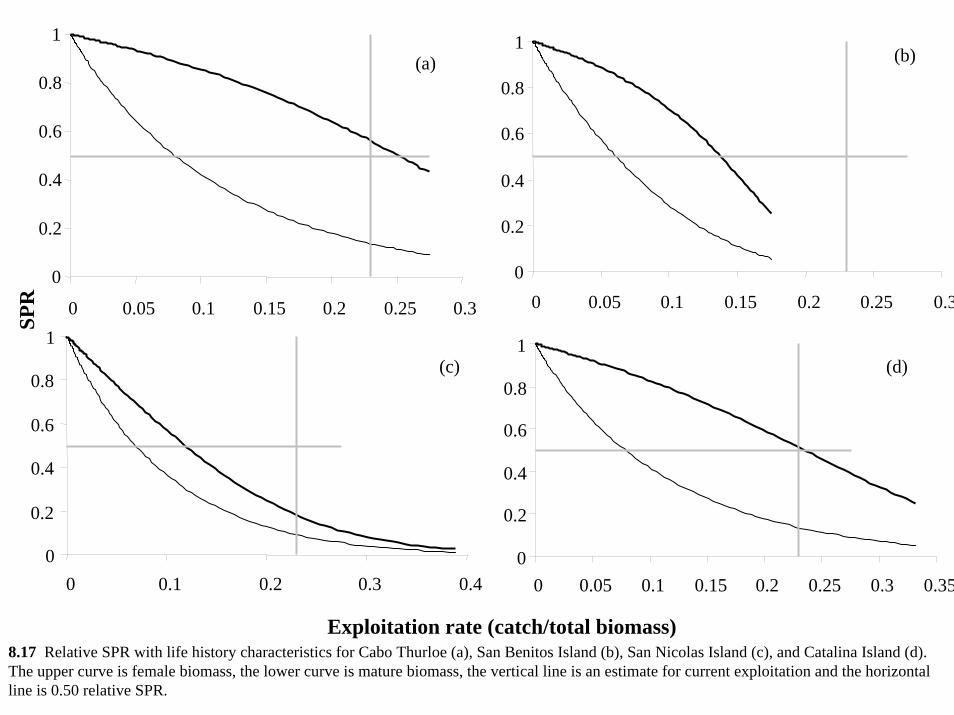
(a)

(c)

(b)

(d)

8.17 Relative SPR with life history characteristics for Cabo Thurloe (a), San Benitos Island (b), San Nicolas Island (c), and Catalina Island (d). The upper curve is female biomass, the lower curve is mature biomass, the vertical line is an estimate for current exploitation and the horizontal line is 0.50 relative SPR.

0

0.2

0.4

0.6

0.8

1

0 0.05 0.1 0.15 0.2 0.25 0.3 0.350

0.2

0.4

0.6

0.8

1

0 0.1 0.2 0.3 0.4

SPR

0

0.2

0.4

0.6

0.8

1

0 0.05 0.1 0.15 0.2 0.25 0.3

0

0.2

0.4

0.6

0.8

1

0 0.05 0.1 0.15 0.2 0.25 0.3

Exploitation rate (catch/total biomass)

12. APPENDICIES

146

APPENDIX 1: The parameter file for the baseline Sheephead model in Synthesis spbase.d13 LOOP1: 8 LIKE: -342.57294 DELTA LIKE: .00025 ENDBIO: 1037. spbase.r01 spbase.p34 Baseline best-fit Sheephead model for the 2004 assessment 100.000000 .001000 BEGIN AND END DELTA F PER LOOP1 3 .95 FIRST LOOP1 FOR LAMBDA & VALUE 1.500 MAX VALUE FOR CROSS DERIVATIVE 1 READ HESSIAN spbase.hes 1 WRITE HESSIAN spbase.hes .001 MIN SAMPLE FRAC. PER AGE 1 20 1 20 MINAGE, MAXAGE, SUMMARY AGE RANGE 1947 2003 BEGIN YEAR, END YEAR 1 12 0 0 0 NPER, MON/PER 6.00 SPAWNMONTH 4 4 NFISHERY, NSURVEY 1 N SEXES 1000. REF RECR LEVEL 0 MORTOPT .350000 .001000 3.000000 'NATMORT ' 0 1 0 .000000 .0000 ! 1 NO PICK .000 -.01 .0000000 HKLINE TYPE: 1 8 SELECTIVITY PATTERN 0 0 0 2 0 0 0 AGE TYPES USED 1.00000 .20 ' HKLINE CATCH ' ! # = 1 VALUE: -.05724 1.00000 .20 ' HKLINE SIZECOMP ' ! # = 2 VALUE: -32.06566 1 0 0 0 0 0 SEL. COMPONENTS .005793 .000100 1.000000 'HKLINE INITIAL S' 2 1 0 .000000 .0000 ! 2 OK .000 -127453.15 .0000099 .999978 .000100 1.000000 'HKLINE INFLECT ' 2 1 0 .000000 .0000 ! 3 OK .000************** .0000000 .308123 .000100 5.000000 'HKLINE SLOPE ' 2 1 0 .000000 .0000 ! 4 OK -.001 -678.28 .0019460 TRAPS TYPE: 2 8 SELECTIVITY PATTERN 0 0 0 4 0 0 0 AGE TYPES USED 1.00000 .20 ' TRAP CATCH ' ! # = 3 VALUE: .00000 1.00000 .20 ' TRAP SIZECOMP ' ! # = 4 VALUE: -42.90195 1 0 0 0 0 0 SEL. COMPONENTS .005481 .000100 1.000000 'TRAPS INITIAL SE' 2 1 0 .000000 .0000 ! 5 OK .000 -56403.75 .0000261 .350618 .000100 1.000000 'TRAP INFLECT ' 2 1 0 .000000 .0000 ! 6 OK .000 -5741.37 .0003282 .689538 .000100 5.000000 'TRAP SLOPE ' 2 1 0 .000000 .0000 ! 7 OK .000 -79.50 .0268074 SETNET TYPE: 3 8 SELECTIVITY PATTERN 0 0 0 6 0 0 0 AGE TYPES USED 1.00000 .20 ' SETNET CATCH ' ! # = 5 VALUE: .00000 1.00000 .20 ' SETNET SIZECOMP ' ! # = 6 VALUE: -12.87307 1 0 0 0 0 0 SEL. COMPONENTS .001891 .000100 1.000000 'SETNET INITIAL S' 2 1 0 .000000 .0000 ! 8 OK .000 -245098.78 .0000049 .999995 .000100 1.000000 'SETNET INFLECT ' 2 1 0 .000000 .0000 ! 9 OK .000************** .0000000 .254941 .000100 5.000000 'SETNET SLOPE ' 2 1 0 .000000 .0000 ! 10 OK .000 -1056.43 .0013201

RECREA TYPE: 4 8 SELECTIVITY PATTERN 0 0 0 8 0 0 0 AGE TYPES USED 1.00000 .20 ' RECREA CATCH ' ! # = 7 VALUE: -.05724 1.00000 .20 ' RECREA SIZECOMP ' ! # = 8 VALUE: -189.16699 1 0 0 0 0 0 SEL. COMPONENTS .001230 .000100 1.000000 'RECREA INITIAL S' 2 1 0 .000000 .0000 ! 11 OK .000 -3000281.69 .0000004 .308864 .010000 1.000000 'RECREA INFLECT ' 2 1 0 .000000 .0000 ! 12 OK .000 -63814.08 .0000950 .536938 .010000 5.000000 'RECREA SLOPE ' 2 1 0 .000000 .0000 ! 13 OK .000 -2673.40 .0010982 CPFV1 TYPE: 5 2 SELECTIVITY PATTERN 0 0 0 0 0 0 0 AGE TYPES USED .000121 0 1 2 Q, QUANT, LOGERROR=1, BIO=1 or NUM=2 1.00000 .20 'CPFV1 Q ' ! # = 9 VALUE: -12.39961 4.000000 -.200000 1.000000 'CPFV1 SELTYPE ' 0 -1947 0 .000000 .0000 ! 14 NO PICK .000 -.01 .0000000 10.000000 .010000 10.000000 'CPFV1 MINSIZE ' 0 -1947 0 .000000 .0000 ! 15 NO PICK .000 -.01 .0000000 100.000000 .001000 100.000000 'CPFV1 MAXSIZE ' 0 -1947 0 .000000 .0000 ! 16 NO PICK .000 -.01 .0000000 CPFV2 TYPE: 6 2 SELECTIVITY PATTERN 0 0 0 0 0 0 0 AGE TYPES USED .000035 0 1 2 Q, QUANT, LOGERROR=1, BIO=1 or NUM=2 1.00000 .20 'CPFV2 Q ' ! # = 10 VALUE: -16.93212 4.000000 -.200000 1.000000 'CPFV2 SELTYPE ' 0 -1960 0 .000000 .0000 ! 17 NO PICK .000 -.01 .0000000 10.000000 .010000 10.000000 'CPFV2 MINSIZE ' 0 -1960 0 .000000 .0000 ! 18 NO PICK .000 -.01 .0000000 100.000000 .001000 100.000000 'CPFV2 MAXSIZE ' 0 -1960 0 .000000 .0000 ! 19 NO PICK .000 -.01 .0000000 CPFV3 TYPE: 7 2 SELECTIVITY PATTERN 0 0 0 0 0 0 0 AGE TYPES USED .001145 0 1 2 Q, QUANT, LOGERROR=1, BIO=1 or NUM=2 1.00000 .20 'CPFV3 Q ' ! # = 11 VALUE: 10.09611 4.000000 -.200000 1.000000 'CPFV3 SELTYPE ' 0 -1980 0 .000000 .0000 ! 20 NO PICK .000 -.01 .0000000 10.000000 .010000 10.000000 'CPFV3 MINSIZE ' 0 -1980 0 .000000 .0000 ! 21 NO PICK .000 -.01 .0000000 100.000000 .001000 100.000000 'CPFV3 MAXSIZE ' 0 -1980 0 .000000 .0000 ! 22 NO PICK .000 -.01 .0000000 CalCOFI TYPE: 8 4 SELECTIVITY PATTERN 0 0 0 0 0 0 0 AGE TYPES USED .000001 0 1 2 Q, QUANT, LOGERROR=1, BIO=1 or NUM=2 1.00000 .20 'CalCOFI SPB ' ! # = 12 VALUE: -46.21517 1 AGEERR: 1: MULTINOMIAL, 0: S(LOG(P))=CONSTANT, -1: S=P*Q/N 200.000 : MAX N FOR MULTINOMIAL 3 1=%CORRECT, 2=C.V., 3=%AGREE, 4=READ %AGREE @AGE .800000 .300000 .950000 '%AGREE @ MIN ' 0 -1980 0 .000000 .0000 ! 23 NO PICK .000 -.01 .0000000 .050000 .000000 .900000 '%AGREE @ MAX ' 0 -1980 0 .000000 .0000 ! 24 NO PICK .000 -.01 .0000000 1.000000 .001000 2.000000 '%AGREE POWER ' 0 -1980 0 .000000 .0000 ! 25 NO PICK .000 -.01 .0000000 .150000 .010000 .300000 'OLD DISCOUNT ' 0 -1980 0 .000000 .0000 ! 26 NO PICK .000 -.01 .0000000 .000000 .001000 .100000 '%MIS_SEXED ' 0 -1980 0 .000000 .0000 ! 27 NO PICK .000 -.01 .0000000 0 END OF EFFORT 0 FIX n FMORTs

2 MATURITY 25.240000 10.000000 100.000000 'MATURITY INFL ' 0 1 0 .000000 .0000 ! 28 NO PICK .000 -.01 .0000000 1.060000 .001000 5.000000 'MATURITY SLOPE ' 0 1 0 .000000 .0000 ! 29 NO PICK .000 -.01 .0000000 .000000 .000000 5.000000 'MATURITY - DD ' 0 1 0 .000000 .0000 ! 30 NO PICK .000 -.01 .0000000 36.700000 10.000000 100.000000 'MATURITY - INFL2' 0 1 0 .000000 .0000 ! 31 NO PICK .000 -.01 .0000000 .320000 .001000 5.000000 'MATURITY - SLP2 ' 0 1 0 .000000 .0000 ! 32 NO PICK .000 -.01 .0000000 1 GROWTH: 1=CONSTANT, 2=MORT. INFLUENCE 1.0000 13.0000 AGE AT WHICH L1 AND L2 OCCUR 1 1=NORMAL, 2=LOGNORMAL 12.920000 1.000000 100.000000 'L1 ' 0 1 0 .000000 .0000 ! 33 NO PICK .000 -.01 .0000000 52.600000 10.000000 100.000000 'LINF ' 0 1 0 .000000 .0000 ! 34 NO PICK .000 -.01 .0000000 .068000 .000100 4.000000 'K ' 0 1 0 .000000 .0000 ! 35 NO PICK .000 -.01 .0000000 .144787 .001000 .290000 'CV1 ' 2 1 0 .000000 .0000 ! 36 OK .000 -16525.43 .0027558 .260825 .001000 .290000 'CV1 ' 2 1 0 .000000 .0000 ! 37 OK -.001 -2272.83 .0140529 0 DEFINE MARKET CATEGORIES 0 ENVIRONMENTAL FXN: [-INDEX] [FXN TYPE(1-4)] [ENVVAR USED] 0 ESTIMATE N ENVIRON VALUES 0 PENALTIES 0 ENVIRONMENT EFFECT ON EXP(RECR) 13 STOCK-RECR 3 1=B-H, 2=RICKER, 3=new B-H, 4=HOCKEY 0 0=recr is mult x averecr, 1=log(DEV) from S-R .00000 -.61 ' SPAWN-RECR-IND ' ! # = 13 VALUE: -2450.28137 .00000 -.30 ' SPAWN-RECR-MEAN ' ! # = 14 VALUE: -267579.98097 1.392113 .200000 15.000000 'VIRGIN RECR MULT' 2 1 0 .000000 .0000 ! 38 OK .000 -1.01 .0000000 .700000 .100000 .990000 'B/H S/R PARAM ' 2 1 0 .000000 .0000 ! 39 OK .000 -1.01 .0000000 .879565 .100000 1000.000000 'BACK. RECRUIT ' 2 1 0 .000000 .0000 ! 40 OK .000 -573.49 .0023595 .610740 .100000 .990000 'S/R STD.DEV. ' 2 1 0 .000000 .0000 ! 41 OK .000 -1.01 .0000000 .000000 -.100000 .100000 'RECR TREND ' 0 1 0 .000000 .0000 ! 42 NO PICK .000 -.01 .0000000 1.000000 .010000 10.000000 'RECR-MULT ' 0 1 0 .000000 .0000 ! 43 NO PICK .000 -.01 .0000000 -2 INIT AGE COMP .10000E-04 .10000E-04 .10000E+04 'RECR 1947 ' 2 1947 0 .00000E+00 .0000 ! 44 BOUND .000 -.01 .0000000 .10000E-04 .10000E-04 .10000E+04 'RECR 1948 ' 2 1948 0 .00000E+00 .0000 ! 45 BOUND .000 -.01 .0000000 .10000E-04 .10000E-04 .10000E+04 'RECR 1949 ' 2 1949 0 .00000E+00 .0000 ! 46 BOUND .000 -.01 .0000000 .379973 .000010 1000.000000 'RECR 1950 ' 2 1950 0 .000000 .0000 ! 47 OK .013 -.32 7.0221005 .908167 .000010 1000.000000 'RECR 1951 ' 2 1951 0 .000000 .0000 ! 48 OK .014 -.33 11.6044858 .258704 .000010 1000.000000 'RECR 1952 ' 2 1952 0 .000000 .0000 ! 49 OK .001 -.37 9.7869974 .10000E-04 .10000E-04 .10000E+04 'RECR 1953 ' 2 1953 0 .00000E+00 .0000 ! 50 BOUND .000 -.01 .0000000 .209285 .000010 1000.000000 'RECR 1954 ' 2 1954 0 .000000 .0000 ! 51 OK .001 -.40 8.9602294 .868467 .000010 1000.000000 'RECR 1955 ' 2 1955 0 .000000 .0000 ! 52 OK -.005 -.38 10.5169026 .256415 .000010 1000.000000 'RECR 1956 ' 2 1956 0 .000000 .0000 ! 53 OK -.003 -.36 13.5930758 .114372 .000010 1000.000000 'RECR 1957 ' 2 1957 0 .000000 .0000 ! 54 OK -.007 -.26 15.0761416 .10000E-04 .10000E-04 .10000E+04 'RECR 1958 ' 2 1958 0 .00000E+00 .0000 ! 55 BOUND .000 -.01 127.7874979 3.843077 .000010 1000.000000 'RECR 1959 ' 2 1959 0 .000000 .0000 ! 56 BIG DX -.052 -.03 81.8756818 3.961665 .000010 1000.000000 'RECR 1960 ' 2 1960 0 .000000 .0000 ! 57 OK -.049 -.02 187.5174318 1.639433 .000010 1000.000000 'RECR 1961 ' 2 1961 0 .000000 .0000 ! 58 BIG DX -.084 -.03 198.3726438 3.557151 .000010 1000.000000 'RECR 1962 ' 2 1962 0 .000000 .0000 ! 59 OK -.045 -.05 116.1409925 3.167107 .000010 1000.000000 'RECR 1963 ' 2 1963 0 .000000 .0000 ! 60 OK -.016 -.08 65.2935513 .10000E-04 .10000E-04 .10000E+04 'RECR 1964 ' 2 1964 0 .00000E+00 .0000 ! 61 BOUND .000 -.01 .0000000 .10000E-04 .10000E-04 .10000E+04 'RECR 1965 ' 2 1965 0 .00000E+00 .0000 ! 62 BOUND .000 -.01 .0000000 .10000E-04 .10000E-04 .10000E+04 'RECR 1966 ' 2 1966 0 .00000E+00 .0000 ! 63 BOUND .000 -.01 .0000000

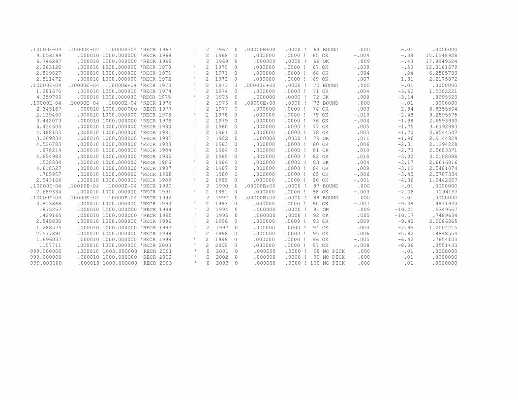
.10000E-04 .10000E-04 .10000E+04 'RECR 1967 ' 2 1967 0 .00000E+00 .0000 ! 64 BOUND .000 -.01 .0000000 4.058199 .000010 1000.000000 'RECR 1968 ' 2 1968 0 .000000 .0000 ! 65 OK -.004 -.38 15.1548928 6.746247 .000010 1000.000000 'RECR 1969 ' 2 1969 0 .000000 .0000 ! 66 OK .009 -.43 17.9949524 2.263120 .000010 1000.000000 'RECR 1970 ' 2 1970 0 .000000 .0000 ! 67 OK -.039 -.50 12.3161679 2.819827 .000010 1000.000000 'RECR 1971 ' 2 1971 0 .000000 .0000 ! 68 OK .004 -.84 6.2505783 2.811472 .000010 1000.000000 'RECR 1972 ' 2 1972 0 .000000 .0000 ! 69 OK -.007 -1.81 2.2175872 .10000E-04 .10000E-04 .10000E+04 'RECR 1973 ' 2 1973 0 .00000E+00 .0000 ! 70 BOUND .000 -.01 .0000000 1.281670 .000010 1000.000000 'RECR 1974 ' 2 1974 0 .000000 .0000 ! 71 OK .004 -3.60 1.5302221 4.359793 .000010 1000.000000 'RECR 1975 ' 2 1975 0 .000000 .0000 ! 72 OK .000 -3.14 .8295523 .10000E-04 .10000E-04 .10000E+04 'RECR 1976 ' 2 1976 0 .00000E+00 .0000 ! 73 BOUND .000 -.01 .0000000 2.345187 .000010 1000.000000 'RECR 1977 ' 2 1977 0 .000000 .0000 ! 74 OK -.003 -2.84 8.8355504 2.139460 .000010 1000.000000 'RECR 1978 ' 2 1978 0 .000000 .0000 ! 75 OK -.010 -2.48 9.2595675 3.442073 .000010 1000.000000 'RECR 1979 ' 2 1979 0 .000000 .0000 ! 76 OK -.004 -1.98 2.6593930 6.434604 .000010 1000.000000 'RECR 1980 ' 2 1980 0 .000000 .0000 ! 77 OK .005 -1.75 3.6192893 4.488103 .000010 1000.000000 'RECR 1981 ' 2 1981 0 .000000 .0000 ! 78 OK .003 -1.70 3.8544547 3.369834 .000010 1000.000000 'RECR 1982 ' 2 1982 0 .000000 .0000 ! 79 OK .011 -1.96 2.9144829 4.526783 .000010 1000.000000 'RECR 1983 ' 2 1983 0 .000000 .0000 ! 80 OK .006 -2.31 2.1294228 .878214 .000010 1000.000000 'RECR 1984 ' 2 1984 0 .000000 .0000 ! 81 OK .010 -2.73 2.5683371 4.654983 .000010 1000.000000 'RECR 1985 ' 2 1985 0 .000000 .0000 ! 82 OK .018 -3.02 3.0108088 .538834 .000010 1000.000000 'RECR 1986 ' 2 1986 0 .000000 .0000 ! 83 OK .004 -3.17 2.6616016 4.618527 .000010 1000.000000 'RECR 1987 ' 2 1987 0 .000000 .0000 ! 84 OK .009 -3.19 2.5481074 .705957 .000010 1000.000000 'RECR 1988 ' 2 1988 0 .000000 .0000 ! 85 OK -.006 -3.45 2.5707334 2.543166 .000010 1000.000000 'RECR 1989 ' 2 1989 0 .000000 .0000 ! 86 OK -.001 -4.36 1.2442657 .10000E-04 .10000E-04 .10000E+04 'RECR 1990 ' 2 1990 0 .00000E+00 .0000 ! 87 BOUND .000 -.01 .0000000 2.689334 .000010 1000.000000 'RECR 1991 ' 2 1991 0 .000000 .0000 ! 88 OK -.003 -7.08 .7294157 .10000E-04 .10000E-04 .10000E+04 'RECR 1992 ' 2 1992 0 .00000E+00 .0000 ! 89 BOUND .000 -.01 .0000000 3.813868 .000010 1000.000000 'RECR 1993 ' 2 1993 0 .000000 .0000 ! 90 OK -.007 -9.09 .4811933 .875257 .000010 1000.000000 'RECR 1994 ' 2 1994 0 .000000 .0000 ! 91 OK .009 -10.01 .5349557 .429165 .000010 1000.000000 'RECR 1995 ' 2 1995 0 .000000 .0000 ! 92 OK .005 -10.17 .7489634 2.545830 .000010 1000.000000 'RECR 1996 ' 2 1996 0 .000000 .0000 ! 93 OK .009 -9.40 2.0086865 1.288574 .000010 1000.000000 'RECR 1997 ' 2 1997 0 .000000 .0000 ! 94 OK .003 -7.95 1.2004215 2.577891 .000010 1000.000000 'RECR 1998 ' 2 1998 0 .000000 .0000 ! 95 OK .006 -5.82 .8848554 1.696037 .000010 1000.000000 'RECR 1999 ' 2 1999 0 .000000 .0000 ! 96 OK -.005 -6.42 .7654103 .107711 .000010 1000.000000 'RECR 2000 ' 2 2000 0 .000000 .0000 ! 97 OK -.008 -8.36 .3551433 -999.000000 .000010 1000.000000 'RECR 2001 ' 0 2001 0 .000000 .0000 ! 98 NO PICK .000 -.01 .0000000 -999.000000 .000010 1000.000000 'RECR 2002 ' 0 2002 0 .000000 .0000 ! 99 NO PICK .000 -.01 .0000000 -999.000000 .000010 1000.000000 'RECR 2003 ' 0 2003 0 .000000 .0000 ! 100 NO PICK .000 -.01 .0000000

sheephead data file for 2004 assessment assembled by Meisha Key & Suzanne Alonzo55.47 1 hkline trap setnet recrea1947 1 87.77 0 0 21.031948 1 45.46 0 0 27.911949 1 28.81 0 0 24.971950 1 30.03 0 0 23.091951 1 27.86 0 0 33.011952 1 16.43 0 0 26.651953 1 16.07 0 0 28.051954 1 13.24 0 0 34.771955 1 5.97 0 0 26.641956 1 2.98 0 0 27.751957 1 5 0 0 28.261958 1 5.16 0 0 33.141959 1 4.64 0 0 31.561960 1 2.15 0 0 22.51961 1 5.72 0 0 28.431962 1 9.22 0 0 25.651963 1 12.71 0 0 33.661964 1 8.13 0 0 47.211965 1 5.51 0 0 71.191966 1 7.25 0 0 89.491967 1 8.9 0 0 72.851968 1 5.78 0 0 57.321969 1 6.03 0 0 84.091970 1 1.73 0 0 67.651971 1 4.02 0 0 65.771972 1 3.21 0 0 58.081973 1 1.39 0 0 78.61974 1 1.69 0 0 52.961975 1 2.74 0 0 53.151976 1 3.78 0 0 57.081977 1 2.91 0 0 49.941978 1 0.94 0.49 3.63 59.481979 1 0.23 0.45 3.32 55.581980 1 0.85 1.08 2.2 143.571981 1 0.36 0.36 5.13 106.971982 1 0.44 0.82 4.08 92.031983 1 0.88 0.34 4.5 155.351984 1 1.96 0.28 9.15 131.21985 1 0.17 0.08 12.67 200.21986 1 0.39 0 12.88 223.31987 1 2.76 0 12.16 108.09

1988 1 2.84 0 10.47 178.841989 1 7.84 0 7.25 64.641990 1 49.6 0 6.54 601991 1 80.43 0 6.66 73.631992 1 111.2 0 6.14 45.51993 1 127.11 11.88 4.33 78.241994 1 27.06 89.92 0.72 121.121995 1 26.4 88.2 0.47 54.521996 1 20.89 92.83 0.68 81.221997 1 22.02 115.69 1.28 59.811998 1 24.79 93.32 0.94 76.511999 1 11.24 46.68 0.9 84.942000 1 15.16 62.31 1.21 100.092001 1 10.96 55.78 1.39 58.852002 1 10.34 43.71 0.66 60.262003 1 10.87 36.98 0.15 68.51

-1 1 1 1 1 1 1 END OF CATCH DATA-1 1 1 1 END OF EFFORTAND CPUE DATA

1947 1 8 5 0.0362 0.4 CPFV Logbook CPUE angler days 1948 1 8 5 0.0423 0.4 CPFV Logbook CPUE angler days 1949 1 8 5 0.0329 0.4 CPFV Logbook CPUE angler days1950 1 8 5 0.0262 0.4 CPFV Logbook CPUE angler days1951 1 8 5 0.0367 0.4 CPFV Logbook CPUE angler days 1952 1 8 5 0.028 0.4 CPFV Logbook CPUE angler days 1953 1 8 5 0.0345 0.4 CPFV Logbook CPUE angler days 1954 1 8 5 0.0404 0.4 CPFV Logbook CPUE angler days1955 1 8 5 0.0284 0.4 CPFV Logbook CPUE angler days1956 1 8 5 0.0283 0.4 CPFV Logbook CPUE angler days1957 1 8 5 0.0282 0.4 CPFV Logbook CPUE angler days1958 1 8 5 0.0352 0.4 CPFV Logbook CPUE angler days1959 1 8 5 0.0308 0.4 CPFV Logbook CPUE angler days1960 1 8 5 0.0224 0.4 CPFV Logbook CPUE angler days1961 1 8 5 0.0307 0.4 CPFV Logbook CPUE angler days 1960 1 8 6 0.0181 0.4 CPFV Logbook CPUE per angler1961 1 8 6 0.0256 0.4 CPFV Logbook CPUE per angler1962 1 8 6 0.0226 0.4 CPFV Logbook CPUE per angler1963 1 8 6 0.0287 0.4 CPFV Logbook CPUE per angler1964 1 8 6 0.0386 0.4 CPFV Logbook CPUE per angler1965 1 8 6 0.0605 0.4 CPFV Logbook CPUE per angler1966 1 8 6 0.0618 0.4 CPFV Logbook CPUE per angler1967 1 8 6 0.0547 0.4 CPFV Logbook CPUE per angler1968 1 8 6 0.0389 0.4 CPFV Logbook CPUE per angler 1969 1 8 6 0.0618 0.4 CPFV Logbook CPUE per angler

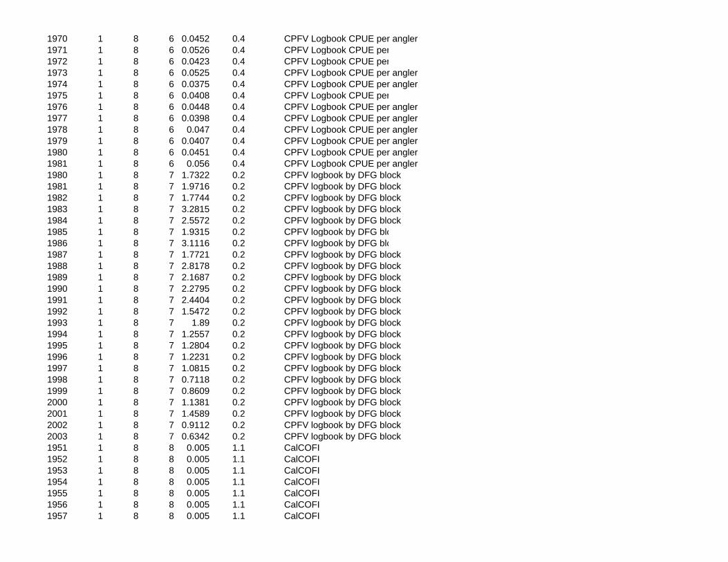
1970 1 8 6 0.0452 0.4 CPFV Logbook CPUE per angler1971 1 8 6 0.0526 0.4 CPFV Logbook CPUE per angler 1972 1 8 6 0.0423 0.4 CPFV Logbook CPUE per angler 1973 1 8 6 0.0525 0.4 CPFV Logbook CPUE per angler 1974 1 8 6 0.0375 0.4 CPFV Logbook CPUE per angler1975 1 8 6 0.0408 0.4 CPFV Logbook CPUE per angler 1976 1 8 6 0.0448 0.4 CPFV Logbook CPUE per angler1977 1 8 6 0.0398 0.4 CPFV Logbook CPUE per angler1978 1 8 6 0.047 0.4 CPFV Logbook CPUE per angler1979 1 8 6 0.0407 0.4 CPFV Logbook CPUE per angler1980 1 8 6 0.0451 0.4 CPFV Logbook CPUE per angler1981 1 8 6 0.056 0.4 CPFV Logbook CPUE per angler1980 1 8 7 1.7322 0.2 CPFV logbook by DFG block1981 1 8 7 1.9716 0.2 CPFV logbook by DFG block1982 1 8 7 1.7744 0.2 CPFV logbook by DFG block1983 1 8 7 3.2815 0.2 CPFV logbook by DFG block1984 1 8 7 2.5572 0.2 CPFV logbook by DFG block1985 1 8 7 1.9315 0.2 CPFV logbook by DFG block 1986 1 8 7 3.1116 0.2 CPFV logbook by DFG block 1987 1 8 7 1.7721 0.2 CPFV logbook by DFG block1988 1 8 7 2.8178 0.2 CPFV logbook by DFG block1989 1 8 7 2.1687 0.2 CPFV logbook by DFG block1990 1 8 7 2.2795 0.2 CPFV logbook by DFG block1991 1 8 7 2.4404 0.2 CPFV logbook by DFG block1992 1 8 7 1.5472 0.2 CPFV logbook by DFG block1993 1 8 7 1.89 0.2 CPFV logbook by DFG block1994 1 8 7 1.2557 0.2 CPFV logbook by DFG block1995 1 8 7 1.2804 0.2 CPFV logbook by DFG block1996 1 8 7 1.2231 0.2 CPFV logbook by DFG block1997 1 8 7 1.0815 0.2 CPFV logbook by DFG block1998 1 8 7 0.7118 0.2 CPFV logbook by DFG block1999 1 8 7 0.8609 0.2 CPFV logbook by DFG block2000 1 8 7 1.1381 0.2 CPFV logbook by DFG block2001 1 8 7 1.4589 0.2 CPFV logbook by DFG block2002 1 8 7 0.9112 0.2 CPFV logbook by DFG block2003 1 8 7 0.6342 0.2 CPFV logbook by DFG block1951 1 8 8 0.005 1.1 CalCOFI 1952 1 8 8 0.005 1.1 CalCOFI 1953 1 8 8 0.005 1.1 CalCOFI 1954 1 8 8 0.005 1.1 CalCOFI 1955 1 8 8 0.005 1.1 CalCOFI 1956 1 8 8 0.005 1.1 CalCOFI 1957 1 8 8 0.005 1.1 CalCOFI

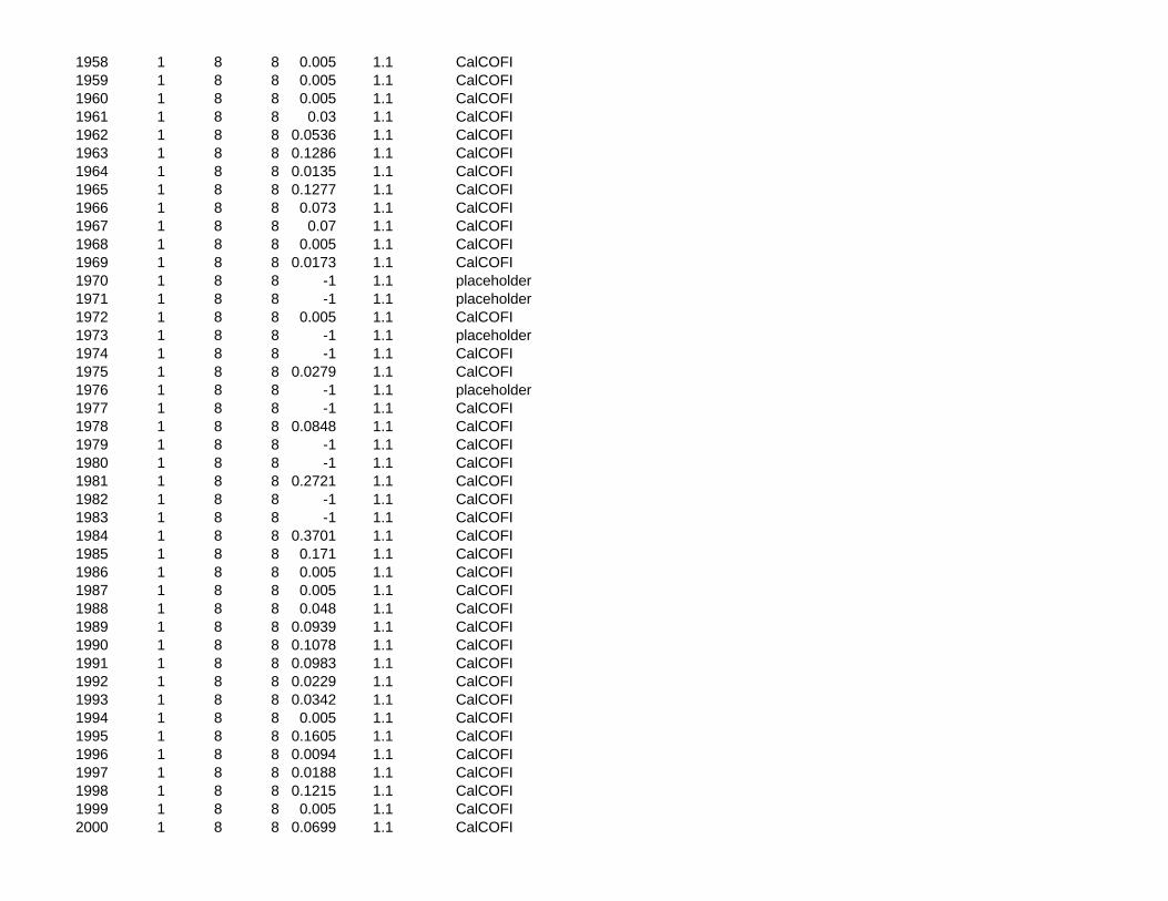
1958 1 8 8 0.005 1.1 CalCOFI 1959 1 8 8 0.005 1.1 CalCOFI 1960 1 8 8 0.005 1.1 CalCOFI 1961 1 8 8 0.03 1.1 CalCOFI 1962 1 8 8 0.0536 1.1 CalCOFI 1963 1 8 8 0.1286 1.1 CalCOFI 1964 1 8 8 0.0135 1.1 CalCOFI 1965 1 8 8 0.1277 1.1 CalCOFI 1966 1 8 8 0.073 1.1 CalCOFI 1967 1 8 8 0.07 1.1 CalCOFI 1968 1 8 8 0.005 1.1 CalCOFI 1969 1 8 8 0.0173 1.1 CalCOFI 1970 1 8 8 -1 1.1 placeholder1971 1 8 8 -1 1.1 placeholder1972 1 8 8 0.005 1.1 CalCOFI 1973 1 8 8 -1 1.1 placeholder 1974 1 8 8 -1 1.1 CalCOFI 1975 1 8 8 0.0279 1.1 CalCOFI 1976 1 8 8 -1 1.1 placeholder1977 1 8 8 -1 1.1 CalCOFI 1978 1 8 8 0.0848 1.1 CalCOFI 1979 1 8 8 -1 1.1 CalCOFI 1980 1 8 8 -1 1.1 CalCOFI 1981 1 8 8 0.2721 1.1 CalCOFI 1982 1 8 8 -1 1.1 CalCOFI 1983 1 8 8 -1 1.1 CalCOFI 1984 1 8 8 0.3701 1.1 CalCOFI 1985 1 8 8 0.171 1.1 CalCOFI 1986 1 8 8 0.005 1.1 CalCOFI 1987 1 8 8 0.005 1.1 CalCOFI 1988 1 8 8 0.048 1.1 CalCOFI 1989 1 8 8 0.0939 1.1 CalCOFI 1990 1 8 8 0.1078 1.1 CalCOFI 1991 1 8 8 0.0983 1.1 CalCOFI 1992 1 8 8 0.0229 1.1 CalCOFI 1993 1 8 8 0.0342 1.1 CalCOFI 1994 1 8 8 0.005 1.1 CalCOFI 1995 1 8 8 0.1605 1.1 CalCOFI 1996 1 8 8 0.0094 1.1 CalCOFI 1997 1 8 8 0.0188 1.1 CalCOFI 1998 1 8 8 0.1215 1.1 CalCOFI 1999 1 8 8 0.005 1.1 CalCOFI 2000 1 8 8 0.0699 1.1 CalCOFI

2001 1 8 8 0.005 1.1 CalCOFI 2002 1 8 8 0.005 1.1 CalCOFI 2003 1 8 8 -1 1.1 CalCOFI

-1 1 1 1 1 1 END OF SURVEY ABUNDANCEDATA-1 -1 (no bins defined for perfect ages)-1 -1 (no bins for imprecise ages)-1 -1 (no bins defined for biased ages)17 17 (17 2-cm length bins [18-50 cm])18 20 22 24 26 28 30 32 34 36 38 40 42 44 46 48 50 83.86

25.2 1.06 length@50%mature, slope (Warner 1975) (could use Cowen 1990 for other estimates)3E-05 2.857 both sexes length-weight (alpha & beta) from deMartini et al. 1994

129 0 eggs/kg on weight (intercept & slope) from deMartini et al. 1994 (could use Warner 1975 instead)3E-05 2.857 both sexes length-weight (alpha & beta) from deMartini et al. 1994

Length compositions 1975 1 4 4 1 79 1 1 17 17 0

0 0 0.0268 0 0.0446 0.0446 0.1339 0.1339 0.1071 0.0625 0.0714 0.0982 0.0804 0.0714 0.0357 0.0357 0.05361976 1 4 4 1 186 1 1 17 17 0

0 0.0038 0.0038 0.0038 0.0113 0.0113 0.0679 0.0792 0.117 0.1434 0.1245 0.0792 0.0981 0.0679 0.0415 0.0415 0.10571977 1 4 4 1 431 1 1 17 17 0

0.0049 0.0016 0.0081 0.0326 0.0765 0.1059 0.1238 0.1238 0.1173 0.0961 0.0586 0.0489 0.0537 0.0244 0.0293 0.0228 0.07171978 1 4 4 1 486 1 1 17 17 0

0.0043 0.0043 0.013 0.0332 0.0506 0.0838 0.1084 0.1084 0.1185 0.0882 0.0607 0.0795 0.0535 0.0419 0.0419 0.0231 0.08671980 1 4 4 1 44 1 1 17 17 0

0 0 0 0.0159 0.0476 0.0635 0.0476 0.0476 0.0794 0.0952 0.0476 0.0317 0.0635 0.0635 0.0476 0.0317 0.31751981 1 4 4 1 58 1 1 17 17 0

0 0.0122 0.0366 0.0244 0.061 0.0488 0.0732 0.122 0.122 0.0732 0.0488 0.0366 0.0488 0.0244 0.0732 0 0.19511982 1 4 4 1 27 1 1 17 17 0

0 0 0 0 0.1026 0.1795 0.1026 0.1795 0.1026 0.1282 0.1538 0.0256 0 0 0 0 0.02561983 1 4 4 1 273 1 1 17 17 0

0 0.0077 0.0077 0.0617 0.0848 0.144 0.1105 0.1465 0.0925 0.0951 0.0771 0.0463 0.0411 0.0257 0.0231 0.0154 0.02061984 1 4 4 1 283 1 1 17 17 0

0.0025 0.0025 0.0223 0.0496 0.1042 0.1117 0.1266 0.1216 0.1216 0.0819 0.1017 0.0397 0.0248 0.0248 0.0223 0.0124 0.02981985 1 4 4 1 381 1 1 17 17 0

0 0 0.0129 0.0221 0.0812 0.1255 0.1255 0.1144 0.1162 0.107 0.0812 0.0664 0.0498 0.0443 0.0148 0.0092 0.02951986 1 4 4 1 534 1 1 17 17 0

0 0.0053 0.0171 0.0315 0.0618 0.0933 0.117 0.1261 0.1209 0.1038 0.0775 0.0631 0.0512 0.0329 0.0184 0.025 0.05521987 1 4 4 1 478 1 1 17 17 0

0 0.0059 0.0132 0.0309 0.0691 0.1 0.1118 0.0765 0.1029 0.0926 0.0897 0.0647 0.0618 0.0397 0.0353 0.0309 0.0751988 1 4 4 1 491 1 1 17 17 0

0 0 0.0029 0.0129 0.0415 0.073 0.073 0.1016 0.0801 0.0801 0.0873 0.0658 0.0644 0.0629 0.0472 0.0372 0.17021989 1 4 4 1 272 1 1 17 17 0

0 0 0.0026 0.0258 0.0672 0.1085 0.1034 0.1085 0.0982 0.1034 0.0982 0.0749 0.0491 0.0388 0.0336 0.0181 0.06981993 1 1 4 1 5 1 1 17 17 0

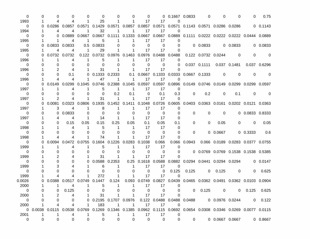
0 0 0 0 0 0 0 0 0 0 0.1667 0.0833 0 0 0 0 0.751993 1 4 4 1 25 1 1 17 17 0

0 0 0.0286 0.0857 0.0571 0.1429 0.0571 0.0857 0.0857 0.0571 0.0571 0.1143 0.0571 0.0286 0.0286 0 0.11431994 1 4 4 1 32 1 1 17 17 0

0 0 0 0.0889 0.0667 0.0667 0.1111 0.1333 0.0667 0.0667 0.0889 0.1111 0.0222 0.0222 0.0222 0.0444 0.08891995 1 1 4 1 5 1 1 17 17 0

0 0 0.0833 0.0833 0.5 0.0833 0 0 0 0 0 0 0.0833 0 0.0833 0 0.08331995 1 4 4 1 29 1 1 17 17 0

0 0 0.0732 0.0732 0.122 0.0732 0.0976 0.1463 0.0976 0.0488 0.0488 0.122 0.0732 0.0244 0 0 01996 1 1 4 1 5 1 1 17 17 0

0 0 0 0 0 0 0 0 0 0 0 0.037 0.1111 0.037 0.1481 0.037 0.62961996 1 2 4 1 31 1 1 17 17 0

0 0 0 0.1 0 0.1333 0.2333 0.1 0.0667 0.1333 0.0333 0.0667 0.1333 0 0 0 01996 1 4 4 1 47 1 1 17 17 0

0 0 0.0149 0.0299 0.1045 0.0746 0.2388 0.1045 0.0597 0.0597 0.0896 0.0149 0.0746 0.0149 0.0299 0.0299 0.05971997 1 1 4 1 5 1 1 17 17 0

0 0 0 0 0 0 0.2 0.1 0 0.1 0.3 0 0.2 0 0.1 0 01997 1 2 4 1 31 1 1 17 17 0

0 0 0.0081 0.0323 0.0806 0.1935 0.1452 0.1411 0.1048 0.0726 0.0605 0.0403 0.0363 0.0161 0.0202 0.0121 0.03631997 1 3 4 1 8 1 1 17 17 0

0 0 0 0.0833 0 0 0 0 0 0 0 0 0 0 0 0.0833 0.83331997 1 4 4 1 14 1 1 17 17 0

0 0 0 0.15 0.05 0.15 0.25 0.05 0.1 0.05 0.1 0 0 0.05 0 0 0.051998 1 1 4 1 5 1 1 17 17 0

0 0 0 0 0 0 0 0 0 0 0 0 0 0.0667 0 0.3333 0.61998 1 4 4 1 74 1 1 17 17 0

0 0 0.0094 0.0472 0.0755 0.1604 0.1226 0.0283 0.1038 0.066 0.066 0.0943 0.066 0.0189 0.0283 0.0377 0.07551999 1 1 4 1 5 1 1 17 17 0

0 0 0 0 0 0 0 0 0 0 0 0 0.0769 0.0769 0.1538 0.1538 0.53851999 1 2 4 1 31 1 1 17 17 0

0 0 0 0 0 0.0588 0.2353 0.25 0.1618 0.0588 0.0882 0.0294 0.0441 0.0294 0.0294 0 0.01471999 1 3 4 1 6 1 1 17 17 0

0 0 0 0 0 0 0 0 0 0 0.125 0.125 0 0.125 0 0 0.6251999 1 4 4 1 272 1 1 17 17 0

0.0026 0 0.0388 0.0517 0.0749 0.1447 0.124 0.093 0.0749 0.0827 0.0439 0.0465 0.0362 0.0491 0.0362 0.0103 0.09042000 1 1 4 1 5 1 1 17 17 0

0 0 0 0.125 0 0 0 0 0 0 0 0 0.125 0 0 0.125 0.6252000 1 2 4 1 31 1 1 17 17 0

0 0 0 0 0 0.2195 0.1707 0.0976 0.122 0.0488 0.0488 0.0488 0 0.0976 0.0244 0 0.1222000 1 4 4 1 183 1 1 17 17 0

0 0.0038 0.0115 0.0538 0.0769 0.1269 0.1346 0.1385 0.0962 0.1115 0.0692 0.0654 0.0308 0.0346 0.0269 0.0077 0.01152001 1 1 4 1 5 1 1 17 17 0

0 0 0 0 0 0 0 0 0 0 0 0 0 0.0667 0.0667 0 0.8667

2001 1 2 4 1 31 1 1 17 17 00 0 0 0 0 0 0.1018 0.1614 0.1333 0.1228 0.0807 0.0772 0.0772 0.0491 0.0526 0.0211 0.1228

2001 1 3 4 1 26 1 1 17 17 00 0 0 0 0.0263 0.0789 0.0526 0.0263 0.0789 0 0.0526 0.0789 0.0263 0.0789 0.1842 0.0263 0.2895

2001 1 4 4 1 101 1 1 17 17 00 0 0 0.0069 0.0417 0.125 0.2153 0.1458 0.1181 0.0764 0.0764 0.0625 0.0694 0.0069 0.0278 0.0069 0.0208

2002 1 2 4 1 31 1 1 17 17 00 0 0 0 0 0.0058 0.0526 0.117 0.1053 0.0994 0.1228 0.0409 0.0643 0.0877 0.0819 0.076 0.1462

2002 1 4 4 1 129 1 1 17 17 00 0 0 0.0109 0.0326 0.0707 0.1848 0.1522 0.1522 0.1196 0.087 0.0489 0.0326 0.0326 0.0217 0.0163 0.038

2003 1 1 4 1 5 1 1 17 17 00 0 0 0 0 0 0 0 0 0.1429 0 0 0 0.2857 0 0 0.5714

2003 1 2 4 1 31 1 1 17 17 00 0 0 0 0 0 0.0814 0.2127 0.1991 0.1719 0.0633 0.0633 0.0724 0.0181 0.0452 0.0362 0.0362

2003 1 4 4 1 195 1 1 17 17 00 0 0 0 0.0072 0.0578 0.2383 0.1805 0.1552 0.083 0.0686 0.0578 0.0578 0.0433 0.0181 0.0072 0.0253

APPENDIX 3: The parameter file for the Review Panel baseline Sheephead model in Synthesis panel.d02 LOOP1: 7 LIKE: -423.56754 DELTA LIKE: .00020 ENDBIO: 239. panel.r01 panel.p11 stage 2 changes requested by panel- virgin recruits, new baseline model search ascending only fir 100.000000 .001000 BEGIN AND END DELTA F PER LOOP1 3 .95 FIRST LOOP1 FOR LAMBDA & VALUE 1.500 MAX VALUE FOR CROSS DERIVATIVE 1 READ HESSIAN spbase.hes 1 WRITE HESSIAN spbase.hes .001 MIN SAMPLE FRAC. PER AGE 1 20 7 20 MINAGE, MAXAGE, SUMMARY AGE RANGE 1947 2003 BEGIN YEAR, END YEAR 1 12 0 0 0 NPER, MON/PER 6.00 SPAWNMONTH 4 4 NFISHERY, NSURVEY 1 N SEXES 1000. REF RECR LEVEL 0 MORTOPT .20000 .001000 3.000000 'NATMORT ' 0 1 0 .000000 .0000 ! 1 NO PICK .000 -.01 .0000000 HKLINE TYPE: 1 8 SELECTIVITY PATTERN 0 0 0 2 0 0 0 AGE TYPES USED 1.00000 .20 ' HKLINE CATCH ' ! # = 1 VALUE: .00000 1.00000 .20 ' HKLINE SIZECOMP ' ! # = 2 VALUE: -46.77540 1 0 0 0 0 0 SEL. COMPONENTS .007365 .000100 1.000000 'HKLINE INITIAL S' 2 1 0 .000000 .0000 ! 2 OK .000 -88714.10 .0000164 .520713 .000100 1.000000 'HKLINE INFLECT ' 2 1 0 .000000 .0000 ! 3 OK .000 -1274.55 .0018583 .302354 .000100 5.000000 'HKLINE SLOPE ' 2 1 0 .000000 .0000 ! 4 OK .000 -317.86 .0069934 TRAPS TYPE: 2 8 SELECTIVITY PATTERN 0 0 0 4 0 0 0 AGE TYPES USED 1.00000 .20 ' TRAP CATCH ' ! # = 3 VALUE: .00000 1.00000 .20 ' TRAP SIZECOMP ' ! # = 4 VALUE: -50.68638 1 0 0 0 0 0 SEL. COMPONENTS .011185 .000100 1.000000 'TRAPS INITIAL SE' 2 1 0 .000000 .0000 ! 5 OK .000 -17408.33 .0000846 .178000 .000100 1.000000 'TRAP INFLECT ' 2 1 0 .000000 .0000 ! 6 OK .000 -19389.62 .0000787 .752285 .000100 5.000000 'TRAP SLOPE ' 2 1 0 .000000 .0000 ! 7 OK .000 -39.55 .0476835 SETNET TYPE: 3 8 SELECTIVITY PATTERN 0 0 0 6 0 0 0 AGE TYPES USED 1.00000 .20 ' SETNET CATCH ' ! # = 5 VALUE: .00000 1.00000 .20 ' SETNET SIZECOMP ' ! # = 6 VALUE: -24.76985 1 0 0 0 0 0 SEL. COMPONENTS .000612 .000100 1.000000 'SETNET INITIAL S' 2 1 0 .000000 .0000 ! 8 OK .000 -1067543.78 .0000012 .656452 .000100 1.000000 'SETNET INFLECT ' 2 1 0 .000000 .0000 ! 9 OK .000 -296.55 .0091487 .179861 .000100 5.000000 'SETNET SLOPE ' 2 1 0 .000000 .0000 ! 10 OK .000 -2802.16 .0010298 RECREA TYPE: 4 8 SELECTIVITY PATTERN 0 0 0 8 0 0 0 AGE TYPES USED 1.00000 .20 ' RECREA CATCH ' ! # = 7 VALUE: .00000 1.00000 .20 ' RECREA SIZECOMP ' ! # = 8 VALUE: -238.95360 1 0 0 0 0 0 SEL. COMPONENTS .002149 .000100 1.000000 'RECREA INITIAL S' 2 1 0 .000000 .0000 ! 11 OK .000 -846539.13 .0000013 .148960 .010000 1.000000 'RECREA INFLECT ' 2 1 0 .000000 .0000 ! 12 OK .000 -216535.95 .0000100 .562873 .010000 5.000000 'RECREA SLOPE ' 2 1 0 .000000 .0000 ! 13 OK .000 -1521.75 .0012841 CPFV1 TYPE: 5

2 SELECTIVITY PATTERN 0 0 0 0 0 0 0 AGE TYPES USED .000083 0 1 2 Q, QUANT, LOGERROR=1, BIO=1 or NUM=2 1.00000 .20 'CPFV1 Q ' ! # = 9 VALUE: -12.25646 4.000000 -.200000 1.000000 'CPFV1 SELTYPE ' 0 -1947 0 .000000 .0000 ! 14 NO PICK .000 -.01 .0000000 10.000000 .010000 10.000000 'CPFV1 MINSIZE ' 0 -1947 0 .000000 .0000 ! 15 NO PICK .000 -.01 .0000000 100.000000 .001000 100.000000 'CPFV1 MAXSIZE ' 0 -1947 0 .000000 .0000 ! 16 NO PICK .000 -.01 .0000000 CPFV2 TYPE: 6 2 SELECTIVITY PATTERN 0 0 0 0 0 0 0 AGE TYPES USED .000069 0 1 2 Q, QUANT, LOGERROR=1, BIO=1 or NUM=2 1.00000 .20 'CPFV2 Q ' ! # = 10 VALUE: -16.82161 4.000000 -.200000 1.000000 'CPFV2 SELTYPE ' 0 -1960 0 .000000 .0000 ! 17 NO PICK .000 -.01 .0000000 10.000000 .010000 10.000000 'CPFV2 MINSIZE ' 0 -1960 0 .000000 .0000 ! 18 NO PICK .000 -.01 .0000000 100.000000 .001000 100.000000 'CPFV2 MAXSIZE ' 0 -1960 0 .000000 .0000 ! 19 NO PICK .000 -.01 .0000000 CPFV3 TYPE: 7 2 SELECTIVITY PATTERN 0 0 0 0 0 0 0 AGE TYPES USED .001813 0 1 2 Q, QUANT, LOGERROR=1, BIO=1 or NUM=2 1.00000 .20 'CPFV3 Q ' ! # = 11 VALUE: 4.56110 4.000000 -.200000 1.000000 'CPFV3 SELTYPE ' 0 -1980 0 .000000 .0000 ! 20 NO PICK .000 -.01 .0000000 10.000000 .010000 10.000000 'CPFV3 MINSIZE ' 0 -1980 0 .000000 .0000 ! 21 NO PICK .000 -.01 .0000000 100.000000 .001000 100.000000 'CPFV3 MAXSIZE ' 0 -1980 0 .000000 .0000 ! 22 NO PICK .000 -.01 .0000000 CalCOFI TYPE: 8 4 SELECTIVITY PATTERN 0 0 0 0 0 0 0 AGE TYPES USED .000002 0 1 2 Q, QUANT, LOGERROR=1, BIO=1 or NUM=2 1.00000 .20 'CalCOFI SPB ' ! # = 12 VALUE: -34.43127 1 AGEERR: 1: MULTINOMIAL, 0: S(LOG(P))=CONSTANT, -1: S=P*Q/N 200.000 : MAX N FOR MULTINOMIAL 3 1=%CORRECT, 2=C.V., 3=%AGREE, 4=READ %AGREE @AGE .800000 .300000 .950000 '%AGREE @ MIN ' 0 -1980 0 .000000 .0000 ! 23 NO PICK .000 -.01 .0000000 .050000 .000000 .900000 '%AGREE @ MAX ' 0 -1980 0 .000000 .0000 ! 24 NO PICK .000 -.01 .0000000 1.000000 .001000 2.000000 '%AGREE POWER ' 0 -1980 0 .000000 .0000 ! 25 NO PICK .000 -.01 .0000000 .150000 .010000 .300000 'OLD DISCOUNT ' 0 -1980 0 .000000 .0000 ! 26 NO PICK .000 -.01 .0000000 .000000 .001000 .100000 '%MIS_SEXED ' 0 -1980 0 .000000 .0000 ! 27 NO PICK .000 -.01 .0000000 0 END OF EFFORT 0 FIX n FMORTs 2 MATURITY 25.240000 10.000000 100.000000 'MATURITY INFL ' 0 1 0 .000000 .0000 ! 28 NO PICK .000 -.01 .0000000 1.060000 .001000 5.000000 'MATURITY SLOPE ' 0 1 0 .000000 .0000 ! 29 NO PICK .000 -.01 .0000000 .000000 .000000 5.000000 'MATURITY - DD ' 0 1 0 .000000 .0000 ! 30 NO PICK .000 -.01 .0000000 36.700000 10.000000 100.000000 'MATURITY - INFL2' 0 1 0 .000000 .0000 ! 31 NO PICK .000 -.01 .0000000 .320000 .001000 5.000000 'MATURITY - SLP2 ' 0 1 0 .000000 .0000 ! 32 NO PICK .000 -.01 .0000000 1 GROWTH: 1=CONSTANT, 2=MORT. INFLUENCE 1.0000 13.0000 AGE AT WHICH L1 AND L2 OCCUR 1 1=NORMAL, 2=LOGNORMAL 12.920000 1.000000 100.000000 'L1 ' 0 1 0 .000000 .0000 ! 33 NO PICK .000 -.01 .0000000 52.600000 10.000000 100.000000 'LINF ' 0 1 0 .000000 .0000 ! 34 NO PICK .000 -.01 .0000000 .068000 .000100 4.000000 'K ' 0 1 0 .000000 .0000 ! 35 NO PICK .000 -.01 .0000000 .110000 .001000 .290000 'CV1 ' 0 1 0 .000000 .0000 ! 36 NO PICK .000 -.01 .0000000 .110000 .001000 .290000 'CV1 ' 0 1 0 .000000 .0000 ! 37 NO PICK .000 -.01 .0000000 0 DEFINE MARKET CATEGORIES 0 ENVIRONMENTAL FXN: [-INDEX] [FXN TYPE(1-4)] [ENVVAR USED] 0 ESTIMATE N ENVIRON VALUES 0 PENALTIES 0 ENVIRONMENT EFFECT ON EXP(RECR) 13 STOCK-RECR 3 1=B-H, 2=RICKER, 3=new B-H, 4=HOCKEY 0 0=recr is mult x averecr, 1=log(DEV) from S-R

.01000 -.80 ' SPAWN-RECR-IND ' ! # = 13 VALUE: -31.05687 .01000 -.30 ' SPAWN-RECR-MEAN ' ! # = 14 VALUE: -312.34996 .219875 .200000 15.000000 'VIRGIN RECR MULT' 2 1 0 .000000 .0000 ! 38 OK .000 -1476.24 .0011552 .990000 .100000 .990000 'B/H S/R PARAM ' 0 1 0 .000000 .0000 ! 39 NO PICK .000 -.01 .0000000 1.163816 .100000 1000.000000 'BACK. RECRUIT ' 0 1 0 .000000 .0000 ! 40 NO PICK .000 -.01 .0000000 .800000 .100000 .990000 'S/R STD.DEV. ' 0 1 0 .000000 .0000 ! 41 NO PICK .000 -.01 .0000000 .000000 -.100000 .100000 'RECR TREND ' 0 1 0 .000000 .0000 ! 42 NO PICK .000 -.01 .0000000 1.000000 .010000 10.000000 'RECR-MULT ' 0 1 0 .000000 .0000 ! 43 NO PICK .000 -.01 .0000000 -1 INIT AGE COMP .122439 .000010 1000.000000 'RECR 1947 ' 2 1947 0 .000000 .0000 ! 44 OK .000 -17.97 .0682950 .130241 .000010 1000.000000 'RECR 1948 ' 2 1948 0 .000000 .0000 ! 45 OK .000 -15.57 .0804081 .138544 .000010 1000.000000 'RECR 1949 ' 2 1949 0 .000000 .0000 ! 46 OK .000 -13.68 .0986575 .146323 .000010 1000.000000 'RECR 1950 ' 2 1950 0 .000000 .0000 ! 47 OK .000 -12.53 .1149593 .151967 .000010 1000.000000 'RECR 1951 ' 2 1951 0 .000000 .0000 ! 48 OK .000 -12.15 .1289720 .151368 .000010 1000.000000 'RECR 1952 ' 2 1952 0 .000000 .0000 ! 49 OK .000 -13.03 .1300624 .153277 .000010 1000.000000 'RECR 1953 ' 2 1953 0 .000000 .0000 ! 50 OK .000 -13.72 .1376645 .159185 .000010 1000.000000 'RECR 1954 ' 2 1954 0 .000000 .0000 ! 51 OK .000 -14.19 .1471341 .164010 .000010 1000.000000 'RECR 1955 ' 2 1955 0 .000000 .0000 ! 52 OK .000 -14.89 .1624994 .160454 .000010 1000.000000 'RECR 1956 ' 2 1956 0 .000000 .0000 ! 53 OK .000 -17.30 .1438551 .147861 .000010 1000.000000 'RECR 1957 ' 2 1957 0 .000000 .0000 ! 54 OK .000 -21.13 .1134823 .139406 .000010 1000.000000 'RECR 1958 ' 2 1958 0 .000000 .0000 ! 55 OK .000 -24.91 .0953660 .129684 .000010 1000.000000 'RECR 1959 ' 2 1959 0 .000000 .0000 ! 56 OK .000 -29.29 .0827939 1.612239 .000010 1000.000000 'RECR 1960 ' 2 1960 0 .000000 .0000 ! 57 OK -.001 -18.21 .3101900 .123475 .000010 1000.000000 'RECR 1961 ' 2 1961 0 .000000 .0000 ! 58 OK .000 -35.81 .0669103 .128971 .000010 1000.000000 'RECR 1962 ' 2 1962 0 .000000 .0000 ! 59 OK .000 -36.28 .0714022 .139058 .000010 1000.000000 'RECR 1963 ' 2 1963 0 .000000 .0000 ! 60 OK .000 -36.64 .0813681 .136999 .000010 1000.000000 'RECR 1964 ' 2 1964 0 .000000 .0000 ! 61 OK .000 -40.45 .0731628 .138859 .000010 1000.000000 'RECR 1965 ' 2 1965 0 .000000 .0000 ! 62 OK .000 -43.54 .0700242 .790001 .000010 1000.000000 'RECR 1966 ' 2 1966 0 .000000 .0000 ! 63 OK .000 -36.85 .1508386 .145598 .000010 1000.000000 'RECR 1967 ' 2 1967 0 .000000 .0000 ! 64 OK .000 -49.97 .0688721 1.294809 .000010 1000.000000 'RECR 1968 ' 2 1968 0 .000000 .0000 ! 65 OK .000 -45.76 .1019342 .123705 .000010 1000.000000 'RECR 1969 ' 2 1969 0 .000000 .0000 ! 66 OK .000 -66.29 .0422911 .116657 .000010 1000.000000 'RECR 1970 ' 2 1970 0 .000000 .0000 ! 67 OK .000 -75.24 .0356947 1.158491 .000010 1000.000000 'RECR 1971 ' 2 1971 0 .000000 .0000 ! 68 OK .000 -73.55 .0404156 .111973 .000010 1000.000000 'RECR 1972 ' 2 1972 0 .000000 .0000 ! 69 OK .000 -146.43 .0183111 .097487 .000010 1000.000000 'RECR 1973 ' 2 1973 0 .000000 .0000 ! 70 OK .000 -185.07 .0134824 .754900 .000010 1000.000000 'RECR 1974 ' 2 1974 0 .000000 .0000 ! 71 OK .000 -124.66 .0216837 .315519 .000010 1000.000000 'RECR 1975 ' 2 1975 0 .000000 .0000 ! 72 OK .000 -108.62 .0272001 .397883 .000010 1000.000000 'RECR 1976 ' 2 1976 0 .000000 .0000 ! 73 OK .000 -81.65 .0388832 1.023903 .000010 1000.000000 'RECR 1977 ' 2 1977 0 .000000 .0000 ! 74 OK .000 -62.89 .0644968 .353467 .000010 1000.000000 'RECR 1978 ' 2 1978 0 .000000 .0000 ! 75 OK -.001 -59.83 .0736734 1.631827 .000010 1000.000000 'RECR 1979 ' 2 1979 0 .000000 .0000 ! 76 OK .000 -56.98 .0757378 1.168362 .000010 1000.000000 'RECR 1980 ' 2 1980 0 .000000 .0000 ! 77 OK -.001 -60.83 .0687749 .939448 .000010 1000.000000 'RECR 1981 ' 2 1981 0 .000000 .0000 ! 78 OK .000 -68.60 .0569848 1.467415 .000010 1000.000000 'RECR 1982 ' 2 1982 0 .000000 .0000 ! 79 OK .000 -82.06 .0470863 .276011 .000010 1000.000000 'RECR 1983 ' 2 1983 0 .000000 .0000 ! 80 OK .000 -98.92 .0394011 1.230623 .000010 1000.000000 'RECR 1984 ' 2 1984 0 .000000 .0000 ! 81 OK .000 -113.38 .0364135 .370393 .000010 1000.000000 'RECR 1985 ' 2 1985 0 .000000 .0000 ! 82 OK .000 -132.94 .0321506 .916670 .000010 1000.000000 'RECR 1986 ' 2 1986 0 .000000 .0000 ! 83 OK .000 -143.72 .0339520 .475524 .000010 1000.000000 'RECR 1987 ' 2 1987 0 .000000 .0000 ! 84 OK .000 -154.02 .0375689 .240262 .000010 1000.000000 'RECR 1988 ' 2 1988 0 .000000 .0000 ! 85 OK .000 -166.74 .0363572 .199216 .000010 1000.000000 'RECR 1989 ' 2 1989 0 .000000 .0000 ! 86 OK .000 -183.44 .0317055 .631694 .000010 1000.000000 'RECR 1990 ' 2 1990 0 .000000 .0000 ! 87 OK .000 -191.65 .0305949 .341172 .000010 1000.000000 'RECR 1991 ' 2 1991 0 .000000 .0000 ! 88 OK .000 -199.47 .0272552 .456879 .000010 1000.000000 'RECR 1992 ' 2 1992 0 .000000 .0000 ! 89 OK .000 -200.63 .0255811 .952528 .000010 1000.000000 'RECR 1993 ' 2 1993 0 .000000 .0000 ! 90 OK .000 -196.20 .0214115 .070550 .000010 1000.000000 'RECR 1994 ' 2 1994 0 .000000 .0000 ! 91 OK .000 -273.20 .0091046 .768997 .000010 1000.000000 'RECR 1995 ' 2 1995 0 .000000 .0000 ! 92 OK .000 -178.19 .0175815 .360388 .000010 1000.000000 'RECR 1996 ' 2 1996 0 .000000 .0000 ! 93 OK .000 -163.99 .0208137 .713896 .000010 1000.000000 'RECR 1997 ' 2 1997 0 .000000 .0000 ! 94 OK .000 -128.97 .0245946

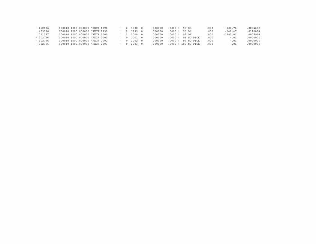
.462676 .000010 1000.000000 'RECR 1998 ' 2 1998 0 .000000 .0000 ! 95 OK .000 -100.76 .0234682 .459330 .000010 1000.000000 'RECR 1999 ' 2 1999 0 .000000 .0000 ! 96 OK .000 -142.47 .0110084 .021097 .000010 1000.000000 'RECR 2000 ' 2 2000 0 .000000 .0000 ! 97 OK .000 -1983.01 .0005914 -.302796 .000010 1000.000000 'RECR 2001 ' 0 2001 0 .000000 .0000 ! 98 NO PICK .000 -.01 .0000000 -.302796 .000010 1000.000000 'RECR 2002 ' 0 2002 0 .000000 .0000 ! 99 NO PICK .000 -.01 .0000000 -.302796 .000010 1000.000000 'RECR 2003 ' 0 2003 0 .000000 .0000 ! 100 NO PICK .000 -.01 .0000000

APPENDIX 4: The data file for the Review Panel baseline Sheephead model in Synthesis "sheephead data file for 2004 assessment, assembled by Meisha Key & Suzanne Alonzo" 55.47 1 hkline trap setnet recrea 1947 1 87.77 0 0 21.03 1948 1 45.46 0 0 27.91 1949 1 28.81 0 0 24.97 NEW VERSION OF THE DATA FILE FOR THE PANEL 1950 1 30.03 0 0 23.09 SAME AS SPBASE.D13 EXCEPT LENGTH COMPOSITION 1951 1 27.86 0 0 33.01 ARE NOT BINNED ABOVE 50CM 1952 1 16.43 0 0 26.65 1953 1 16.07 0 0 28.05 1954 1 13.24 0 0 34.77 1955 1 5.97 0 0 26.64 1956 1 2.98 0 0 27.75 1957 1 5 0 0 28.26 1958 1 5.16 0 0 33.14 1959 1 4.64 0 0 31.56 1960 1 2.15 0 0 22.5 1961 1 5.72 0 0 28.43 1962 1 9.22 0 0 25.65 1963 1 12.71 0 0 33.66 1964 1 8.13 0 0 47.21 1965 1 5.51 0 0 71.19 1966 1 7.25 0 0 89.49 1967 1 8.9 0 0 72.85 1968 1 5.78 0 0 57.32 1969 1 6.03 0 0 84.09 1970 1 1.73 0 0 67.65 1971 1 4.02 0 0 65.77 1972 1 3.21 0 0 58.08 1973 1 1.39 0 0 78.6 1974 1 1.69 0 0 52.96 1975 1 2.74 0 0 53.15 1976 1 3.78 0 0 57.08 1977 1 2.91 0 0 49.94 1978 1 0.94 0.49 3.63 59.48 1979 1 0.23 0.45 3.32 55.58 1980 1 0.85 1.08 2.2 143.57 1981 1 0.36 0.36 5.13 106.97 1982 1 0.44 0.82 4.08 92.03 1983 1 0.88 0.34 4.5 155.35 1984 1 1.96 0.28 9.15 131.2 1985 1 0.17 0.08 12.67 200.2 1986 1 0.39 0 12.88 223.3 1987 1 2.76 0 12.16 108.09 1988 1 2.84 0 10.47 178.84 1989 1 7.84 0 7.25 64.64 1990 1 49.6 0 6.54 60 1991 1 80.43 0 6.66 73.63 1992 1 111.2 0 6.14 45.5 1993 1 127.11 11.88 4.33 78.24 1994 1 27.06 89.92 0.72 121.12 1995 1 26.4 88.2 0.47 54.52 1996 1 20.89 92.83 0.68 81.22 1997 1 22.02 115.69 1.28 59.81 1998 1 24.79 93.32 0.94 76.51 1999 1 11.24 46.68 0.9 84.94 2000 1 15.16 62.31 1.21 100.09 2001 1 10.96 55.78 1.39 58.85 2002 1 10.34 43.71 0.66 60.26

2003 1 10.87 36.98 0.15 68.51 -1 1 1 1 1 1 1 OF CATCH DATA -1 1 1 1 OF EFFORT AND CPUE DATA 1947 1 8 5 0.036178903 0.4 1948 1 8 5 0.042331585 0.4 1949 1 8 5 0.032857006 0.4 1950 1 8 5 0.026239105 0.4 1951 1 8 5 0.036656857 0.4 1952 1 8 5 0.028024765 0.4 1953 1 8 5 0.034549713 0.4 1954 1 8 5 0.040397227 0.4 1955 1 8 5 0.028415067 0.4 1956 1 8 5 0.028273841 0.4 1957 1 8 5 0.028171772 0.4 1958 1 8 5 0.035174085 0.4 1959 1 8 5 0.030774256 0.4 1960 1 8 5 0.022355231 0.4 1961 1 8 5 0.030677383 0.4 1960 1 8 6 0.018103586 0.4 1961 1 8 6 0.025609682 0.4 1962 1 8 6 0.022635962 0.4 1963 1 8 6 0.028675825 0.4 1964 1 8 6 0.038568111 0.4 1965 1 8 6 0.060530182 0.4 1966 1 8 6 0.061805134 0.4 1967 1 8 6 0.054705667 0.4 1968 1 8 6 0.038927611 0.4 1969 1 8 6 0.061815297 0.4 1970 1 8 6 0.045188114 0.4 1971 1 8 6 0.052600786 0.4 1972 1 8 6 0.042316728 0.4 1973 1 8 6 0.052532667 0.4 1974 1 8 6 0.037546657 0.4 1975 1 8 6 0.040767219 0.4 1976 1 8 6 0.044756237 0.4 1977 1 8 6 0.039791441 0.4 1978 1 8 6 0.046977309 0.4 1979 1 8 6 0.040688144 0.4 1980 1 8 6 0.045104848 0.4 1981 1 8 6 0.055954773 0.4 1980 1 8 7 1.732179064 0.2 1981 1 8 7 1.971613638 0.2 1982 1 8 7 1.774373126 0.2 1983 1 8 7 3.281535519 0.2 1984 1 8 7 2.557200197 0.2 1985 1 8 7 1.931451602 0.2 1986 1 8 7 3.111646369 0.2 1987 1 8 7 1.772070442 0.2 1988 1 8 7 2.817807005 0.2 1989 1 8 7 2.168732715 0.2 1990 1 8 7 2.279456015 0.2 1991 1 8 7 2.440362891 0.2 1992 1 8 7 1.547237147 0.2 1993 1 8 7 1.890015687 0.2 1994 1 8 7 1.255741401 0.2 1995 1 8 7 1.280379067 0.2 1996 1 8 7 1.223139248 0.2 1997 1 8 7 1.081495203 0.2 1998 1 8 7 0.71177501 0.2 1999 1 8 7 0.860862578 0.2

2000 1 8 7 1.138076258 0.2 2001 1 8 7 1.45894012 0.2 2002 1 8 7 0.911182492 0.2 2003 1 8 7 0.634184694 0.2 1951 1 8 8 -1 1.1 1952 1 8 8 -1 1.1 1953 1 8 8 -1 1.1 1954 1 8 8 -1 1.1 1955 1 8 8 -1 1.1 1956 1 8 8 -1 1.1 1957 1 8 8 -1 1.1 1958 1 8 8 -1 1.1 1959 1 8 8 -1 1.1 1960 1 8 8 -1 1.1 1961 1 8 8 0.02997 1.1 1962 1 8 8 0.05363 1.1 1963 1 8 8 0.12863 1.1 1964 1 8 8 0.01345 1.1 1965 1 8 8 0.12768 1.1 1966 1 8 8 0.073 1.1 1967 1 8 8 0.07004 1.1 1968 1 8 8 0.005 1.1 1969 1 8 8 0.01733 1.1 1970 1 8 8 -1 1.1 1971 1 8 8 -1 1.1 1972 1 8 8 0.005 1.1 1973 1 8 8 -1 1.1 1974 1 8 8 -1 1.1 1975 1 8 8 0.02788 1.1 1976 1 8 8 -1 1.1 1977 1 8 8 -1 1.1 1978 1 8 8 0.08477 1.1 1979 1 8 8 -1 1.1 1980 1 8 8 -1 1.1 1981 1 8 8 0.27208 1.1 1982 1 8 8 -1 1.1 1983 1 8 8 -1 1.1 1984 1 8 8 0.37014 1.1 1985 1 8 8 0.17095 1.1 1986 1 8 8 0.005 1.1 1987 1 8 8 0.005 1.1 1988 1 8 8 0.04798 1.1 1989 1 8 8 0.09385 1.1 1990 1 8 8 0.10783 1.1 1991 1 8 8 0.09826 1.1 1992 1 8 8 0.02285 1.1 1993 1 8 8 0.03417 1.1 1994 1 8 8 0.005 1.1 1995 1 8 8 0.16048 1.1 1996 1 8 8 0.00941 1.1 1997 1 8 8 0.01878 1.1 1998 1 8 8 0.12147 1.1 1999 1 8 8 0.005 1.1 2000 1 8 8 0.06988 1.1 2001 1 8 8 0.005 1.1 2002 1 8 8 0.005 1.1 2003 1 8 8 -1 1.1 -1 1 1 1 1 1 OF SURVEY ABUNDANCE DATA -1 -1 (no bins defined for perfect ages)

-1 -1 (no bins for imprecise ages) -1 -1 (no bins defined for biased ages) 30 30 (30 2-cm length bins [18-50 cm]) 18 20 22 24 26 28 30 34 36 38 40 42 44 46 48 50 52 54 56 58 60 62 64 66 68 70 72 74 78 83.86 25.2 -1.06 "length@50%mature, slope (Warner 1975) (could use Cowen 1990 for other estimates)" 0.000026935 2.857 both sexes length-weight (alpha & beta) from deMartini et al. 1994 129 0 eggs/kg on weight (intercept & slope) from deMartini et al. 1994 (could use Warner 1975 instead) 0.000026935 2.857 both sexes length-weight (alpha & beta) from deMartini et al. 1994 BEGINNING OF SIZE AND AGE COMPOSITION 1975 1 4 4 1 79 1 30 30 0 0 0 0.026785714 0 0.044642857 0.044642857 0.125 0.116071429 0.0625 0.071428571 0.098214286 0.080357143 0.071428571 0.035714286 0.035714286 0.008928571 0.017857143 0.008928571 0.008928571 0 0 0 0.008928571 0 0 0 0 0 0 1976 1 4 4 1 186 1 30 30 0 0 0.003773585 0.003773585 0.003773585 0.011320755 0.011320755 0.056603774 0.113207547 0.150943396 0.124528302 0.079245283 0.098113208 0.067924528 0.041509434 0.037735849 0.041509434 0.018867925 0.018867925 0.01509434 0.003773585 0.011320755 0 0 0 0 0 0 0 0 1977 1 4 4 1 431 1 30 30 0 0.003257329 0.003257329 0.008143322 0.03257329 0.076547231 0.105863192 0.118892508 0.117263844 0.091205212 0.063517915 0.048859935 0.053745928 0.024429967 0.029315961 0.022801303 0.016286645 0.013029316 0.013029316 0.011400651 0.001628664 0.004885993 0.001628664 0.001628664 0 0.003257329 0 0.001628664 0.003257329 0 1978 1 4 4 1 486 1 30 30 0 0.00433526 0.00433526 0.01300578 0.033236994 0.050578035 0.083815029 0.105491329 0.115606936 0.086705202 0.067919075 0.079479769 0.053468208 0.041907514 0.041907514 0.023121387 0.01300578 0.020231214 0.007225434 0.01734104 0.00433526 0.010115607 0.005780347 0.002890173 0 0.002890173 0.001445087 0.001445087 0 0 1980 1 4 4 1 44 1 30 30 0 0 0 0 0.015873016 0.047619048 0.063492063 0.047619048 0.079365079 0.095238095 0.047619048 0.031746032 0.063492063 0.063492063 0.047619048 0.031746032 0.063492063 0.047619048 0.047619048 0.047619048 0.031746032 0.047619048 0 0 0.015873016 0 0 0.015873016 0 0 1981 1 4 4 1 58 1 30 30 0 0 0.012195122 0.036585366 0.024390244 0.06097561 0.048780488 0.073170732 0.12195122 0.073170732 0.048780488 0.036585366 0.048780488 0.024390244 0.073170732 0 0.06097561 0.036585366 0.048780488 0 0.024390244 0.024390244 0 0 0 0 0 0 0 0 1982 1 4 4 1 27 1 30 30 0 0 0 0 0 0.102564103 0.179487179 0.102564103 0.102564103 0.128205128 0.153846154 0.025641026 0 0 0 0 0 0 0 0 0 0 0 0 0.025641026 0 0 0 0 0

1983 1 4 4 1 273 1 30 30 0 0 0.007712082 0.007712082 0.061696658 0.084832905 0.143958869 0.110539846 0.092544987 0.095115681 0.077120823 0.046272494 0.041131105 0.025706941 0.023136247 0.015424165 0.002570694 0.005141388 0.002570694 0.002570694 0 0.002570694 0.002570694 0 0 0.002570694 0 0 0 0 1984 1 4 4 1 283 1 30 30 0 0.00248139 0.00248139 0.022332506 0.049627792 0.104218362 0.111662531 0.126550868 0.121588089 0.081885856 0.101736973 0.039702233 0.024813896 0.024813896 0.022332506 0.012406948 0 0.014888337 0 0.004962779 0.004962779 0.00248139 0 0.00248139 0 0 0 0 0 0 1985 1 4 4 1 381 1 30 30 0 0 0 0.012915129 0.022140221 0.081180812 0.125461255 0.125461255 0.116236162 0.10701107 0.081180812 0.066420664 0.049815498 0.044280443 0.014760148 0.009225092 0.009225092 0.003690037 0.001845018 0.003690037 0.003690037 0.001845018 0 0.001845018 0.001845018 0 0 0 0.001845018 0 1986 1 4 4 1 534 1 30 30 0 0 0.005256242 0.017082786 0.031537451 0.061760841 0.093298292 0.11695138 0.120893561 0.103810775 0.077529566 0.063074901 0.051248357 0.032851511 0.018396846 0.024967148 0.019710907 0.011826544 0.006570302 0.003942181 0.005256242 0.002628121 0 0 0.00131406 0.00131406 0 0 0 0.002628121 1987 1 4 4 1 478 1 30 30 0 0 0.005882353 0.013235294 0.030882353 0.069117647 0.1 0.111764706 0.102941176 0.092647059 0.089705882 0.064705882 0.061764706 0.039705882 0.035294118 0.030882353 0.027941176 0.013235294 0.013235294 0.001470588 0.005882353 0.004411765 0.004411765 0.002941176 0.001470588 0 0 0 0 0 1988 1 4 4 1 491 1 30 30 0 0 0 0.00286123 0.012875536 0.04148784 0.072961373 0.072961373 0.080114449 0.080114449 0.087267525 0.065808298 0.064377682 0.062947067 0.0472103 0.037195994 0.038626609 0.030042918 0.028612303 0.015736767 0.021459227 0.014306152 0.004291845 0.005722461 0.005722461 0.00286123 0.00286123 0 0 0 1989 1 4 4 1 272 1 30 30 0 0 0 0.002583979 0.025839793 0.067183463 0.108527132 0.103359173 0.098191214 0.103359173 0.098191214 0.074935401 0.049095607 0.03875969 0.033591731 0.018087855 0.020671835 0.015503876 0.005167959 0.018087855 0.002583979 0.005167959 0.002583979 0 0 0 0 0 0 0 1993 1 1 4 1 5 1 30 30 0 0 0 0 0 0 0 0 0 0 0.166666667 0.083333333 0 0 0 0 0 0.083333333 0.083333333 0.083333333 0 0 0 0.166666667 0.083333333 0 0 0.083333333 0 0.166666667 1993 1 4 4 1 25 1 30 30 0 0 0 0.028571429 0.085714286 0.057142857 0.142857143 0.057142857 0.085714286 0.057142857 0.057142857 0.114285714 0.057142857 0.028571429 0.028571429 0 0 0.028571429 0.028571429 0.057142857 0 0 0 0 0 0 0 0 0 0 1994 1 4 4 1 32 1 30 30 0 0 0 0 0.088888889 0.066666667 0.066666667 0.111111111 0.066666667 0.066666667 0.088888889 0.111111111 0.022222222 0.022222222 0.022222222 0.044444444 0 0 0.022222222 0.022222222 0.022222222 0 0 0.022222222 0 0 0 0 0 0 1995 1 1 4 1 5 1 30 30 0 0 0 0.083333333 0.083333333 0.5 0.083333333 0 0 0 0 0 0.083333333 0 0.083333333 0 0.083333333 0 0 0 0 0 0 0 0 0 0 0 0 0 1995 1 4 4 1 29 1 30 30 0

0 0 0.073170732 0.073170732 0.12195122 0.073170732 0.097560976 0.097560976 0.048780488 0.048780488 0.12195122 0.073170732 0.024390244 0 0 0 0 0 0 0 0 0 0 0 0 0 0 0 0 1996 1 2 4 1 31 1 30 30 0 0 0 0 0.1 0 0.133333333 0.233333333 0.066666667 0.133333333 0.033333333 0.066666667 0.133333333 0 0 0 0 0 0 0 0 0 0 0 0 0 0 0 0 0 1996 1 1 4 1 5 1 30 30 0 0 0 0 0 0 0 0 0 0 0 0.037037037 0.111111111 0.037037037 0.148148148 0.037037037 0.074074074 0.037037037 0.222222222 0.111111111 0.148148148 0.037037037 0 0 0 0 0 0 0 0 1996 1 4 4 1 47 1 30 30 0 0 0 0.014925373 0.029850746 0.104477612 0.074626866 0.23880597 0.059701493 0.059701493 0.089552239 0.014925373 0.074626866 0.014925373 0.029850746 0.029850746 0.029850746 0.014925373 0 0 0.014925373 0 0 0 0 0 0 0 0 0 1997 1 3 4 1 8 1 30 30 0 0 0 0 0.083333333 0 0 0 0 0 0 0 0 0 0 0.083333333 0 0 0.083333333 0 0.25 0.25 0 0.083333333 0.083333333 0 0 0.083333333 0 0 1997 1 2 4 1 31 1 30 30 0 0 0 0.008064516 0.032258065 0.080645161 0.193548387 0.14516129 0.10483871 0.072580645 0.060483871 0.040322581 0.036290323 0.016129032 0.02016129 0.012096774 0.02016129 0.008064516 0.004032258 0.004032258 0 0 0 0 0 0 0 0 0 0 1997 1 1 4 1 5 1 30 30 0 0 0 0 0 0 0 0.2 0 0.1 0.3 0 0.2 0 0.1 0 0 0 0 0 0 0 0 0 0 0 0 0 0 0 1997 1 4 4 1 14 1 30 30 0 0 0 0 0.15 0.05 0.15 0.25 0.1 0.05 0.1 0 0 0.05 0 0 0.05 0 0 0 0 0 0 0 0 0 0 0 0 0 1998 1 1 4 1 5 1 30 30 0 0 0 0 0 0 0 0 0 0 0 0 0 0.066666667 0 0.333333333 0.133333333 0.2 0 0.133333333 0 0.066666667 0.066666667 0 0 0 0 0 0 0 1998 1 4 4 1 74 1 30 30 0 0 0 0.009433962 0.047169811 0.075471698 0.160377358 0.122641509 0.103773585 0.066037736 0.066037736 0.094339623 0.066037736 0.018867925 0.028301887 0.037735849 0.018867925 0 0.018867925 0.028301887 0.009433962 0 0 0 0 0 0 0 0 0 1999 1 3 4 1 6 1 30 30 0 0 0 0 0 0 0 0 0 0 0.125 0.125 0 0.125 0 0 0.125 0 0.125 0 0 0 0 0 0.25 0 0 0.125 0 0 1999 1 2 4 1 31 1 30 30 0 0 0 0 0 0 0.058823529 0.235294118 0.161764706 0.058823529 0.088235294 0.029411765 0.044117647 0.029411765 0.029411765 0 0 0 0 0 0 0 0 0 0 0 0 0 0.014705882 0 1999 1 1 4 1 5 1 30 30 0 0 0 0 0 0 0 0 0 0 0 0 0.076923077 0.076923077 0.153846154 0.153846154 0.153846154 0.076923077 0.076923077 0 0.076923077 0 0.153846154 0 0 0 0 0 0 0

1999 1 4 4 1 272 1 30 30 0 0.002583979 0 0.03875969 0.051679587 0.074935401 0.144702842 0.124031008 0.074935401 0.082687339 0.043927649 0.046511628 0.036175711 0.049095607 0.036175711 0.010335917 0.010335917 0.010335917 0.012919897 0.018087855 0.020671835 0.002583979 0.005167959 0.005167959 0.005167959 0 0 0 0 0 2000 1 2 4 1 31 1 30 30 0 0 0 0 0 0 0.219512195 0.170731707 0.12195122 0.048780488 0.048780488 0.048780488 0 0.097560976 0.024390244 0 0.024390244 0 0 0.048780488 0.024390244 0 0.024390244 0 0 0 0 0 0 0 2000 1 1 4 1 5 1 30 30 0 0 0 0 0.125 0 0 0 0 0 0 0 0.125 0 0 0.125 0.125 0.125 0.125 0.125 0 0.125 0 0 0 0 0 0 0 0 2000 1 4 4 1 183 1 30 30 0 0 0.003846154 0.011538462 0.053846154 0.076923077 0.126923077 0.134615385 0.096153846 0.111538462 0.069230769 0.065384615 0.030769231 0.034615385 0.026923077 0.007692308 0.003846154 0.003846154 0.003846154 0 0 0 0 0 0 0 0 0 0 0 2001 1 3 4 1 26 1 30 30 0 0 0 0 0 0.026315789 0.078947368 0.052631579 0.078947368 0 0.052631579 0.078947368 0.026315789 0.078947368 0.184210526 0.026315789 0.052631579 0.131578947 0.052631579 0.026315789 0 0 0 0 0 0.026315789 0 0 0 0 2001 1 2 4 1 31 1 30 30 0 0 0 0 0 0 0 0.101754386 0.133333333 0.122807018 0.080701754 0.077192982 0.077192982 0.049122807 0.052631579 0.021052632 0.024561404 0.024561404 0.024561404 0.028070175 0.010526316 0.003508772 0.007017544 0 0 0 0 0 0 0 2001 1 1 4 1 5 1 30 30 0 0 0 0 0 0 0 0 0 0 0 0 0 0.066666667 0.066666667 0 0 0.266666667 0.066666667 0.066666667 0.066666667 0.133333333 0.066666667 0 0.066666667 0.066666667 0.066666667 0 0 0 2001 1 4 4 1 101 1 30 30 0 0 0 0 0.006944444 0.041666667 0.125 0.215277778 0.118055556 0.076388889 0.076388889 0.0625 0.069444444 0.006944444 0.027777778 0.006944444 0.006944444 0.006944444 0 0.006944444 0 0 0 0 0 0 0 0 0 0 2002 1 2 4 1 31 1 30 30 0 0 0 0 0 0 0.005847953 0.052631579 0.105263158 0.099415205 0.122807018 0.040935673 0.064327485 0.087719298 0.081871345 0.076023392 0.070175439 0.01754386 0.01754386 0.01754386 0.023391813 0 0 0 0 0 0 0 0 0 2002 1 4 4 1 129 1 30 30 0 0 0 0 0.010869565 0.032608696 0.070652174 0.184782609 0.152173913 0.119565217 0.086956522 0.048913043 0.032608696 0.032608696 0.02173913 0.016304348 0.005434783 0 0.010869565 0 0.010869565 0 0 0.005434783 0 0.005434783 0 0 0 0 2003 1 2 4 1 31 1 30 30 0 0 0 0 0 0 0 0.081447964 0.199095023 0.171945701 0.063348416 0.063348416 0.07239819 0.018099548 0.045248869 0.036199095 0.004524887 0 0.009049774 0.004524887 0.009049774 0 0.004524887 0 0.004524887 0 0 0 0 0 2003 1 1 4 1 5 1 30 30 0 0 0 0 0 0 0 0 0 0.142857143 0 0 0 0.285714286 0 0 0.142857143 0.142857143 0 0.142857143 0 0.142857143 0 0 0 0 0 0 0 0

2003 1 4 4 1 195 1 30 30 0 0 0 0 0 0.007220217 0.057761733 0.238267148 0.155234657 0.083032491 0.068592058 0.057761733 0.057761733 0.0433213 0.018050542 0.007220217 0.010830325 0.007220217 0.003610108 0.003610108 0 0 0 0 0 0 0 0 0 0