
Stats 760: Lecture 2
45
© Department of Statistics 2001 Slide 1 Stats 760: Lecture 2
-
Upload
marcia-stephenson -
Category
Documents
-
view
31 -
download
0
description
Stats 760: Lecture 2. Linear Models. Agenda. R formulation Matrix formulation Least squares fit Numerical details – QR decomposition R parameterisations Treatment Sum Helmert. R formulation. Regression model y ~ x1 + x2 + x3 Anova model y ~ A+ B (A, B factors) - PowerPoint PPT Presentation
Transcript of Stats 760: Lecture 2

© Department of Statistics 2001Slide 1
Stats 760: Lecture 2

© Department of Statistics 2001Slide 2
Agenda• R formulation
• Matrix formulation
• Least squares fit
• Numerical details – QR decomposition
• R parameterisations – Treatment– Sum– Helmert

© Department of Statistics 2001Slide 3
R formulation
• Regression model y ~ x1 + x2 + x3
• Anova model y ~ A+ B (A, B factors)
• Model with both factors and continuous variables y ~ A*B*x1 + A*B*x2
What do these mean? How do we interpret the output?

© Department of Statistics 2001Slide 4
Regression model
Mean of observation = 0 + 1x1 + 2x2 + 3x3
Estimate ’s by least squares ie minimize
2
33221101
)(iii
n
ii
xxxy

© Department of Statistics 2001Slide 5
Matrix formulation
nkn
k
n xx
xx
y
y
1
1111
1
1
, X y
Arrange data into a matrix and vector
)()( XbyXby T Then minimise

© Department of Statistics 2001Slide 6
Normal equations
• Minimising b’s satisfy
yXXX TT ̂
)ˆ())ˆ(( )ˆ()ˆ(
)()(
bXbXXyXy
XbyXbyTT
T
Proof: Non-negative, zero when b=beta hat

© Department of Statistics 2001Slide 7
Solving the equations
• We could calculate the matrix XTX directly, but this is not very accurate (subject to roundoff errors). For example, when trying to fit polynomials, this method breaks down for polynomials of low degree
• Better to use the “QR decomposition” which avoids calculating XTX

© Department of Statistics 2001Slide 8
Solving the normal equations
• Use “QR decomposition” X=QR
• X is n x p and must have “full rank” (no column a linear combination of other columns)
• Q is n x p “orthogonal” (i.e. QTQ = identity matrix)
• R is p x p “upper triangular” (all elements below the diagonal zero), all diagonal elements positive, so inverse exists

© Department of Statistics 2001Slide 9
Solving using QRXTX = RTQTQR = RTR
XTy = RTQTy
Normal equations reduce to
RTRb = RTQTy
Premultiply by inverse of RT to get Rb = QTy
Triangular system, easy to solve

© Department of Statistics 2001Slide 10
Solving a triangular system
2231321211
2232322
3333
3
2
1
3
2
1
33
2322
131211
/)(
/)(
/
00
0
rbrbrcb
rbrcb
rcb
c
c
c
b
b
b
r
rr
rrr

© Department of Statistics 2001Slide 11
A refinement• We need QTy:• Solution: do QR decomp of [X,y]
• Thus, solve Rb = r
rQrQqrQQrQyQ
qrQryQRX
r
rRqQyX
TTTT
0
0
0
,
0

© Department of Statistics 2001Slide 12
What R has to do
When you run lm, R forms the matrix X from the model formula, then fits the model E(Y)=Xb
Steps:1. Extract X and Y from the data and the model formula
2. Do the QR decomposition
3. Solve the equations Rb = r
4. Solutions are the numbers reported in the summary

© Department of Statistics 2001Slide 13
Forming X
When all variables are continuous, it’s a no-brainer
1. Start with a column of 1’s
2. Add columns corresponding to the independent variables
It’s a bit harder for factors

© Department of Statistics 2001Slide 14
Factors: one way anova
Consider model y ~ a where a is a factor having 3 levels say.
In this case, we1. Start with a column of ones
2. Add a dummy variable for each level of the factor (3 in all), order is order of factor levels
Problem: matrix has 4 columns, but first is sum of last 3, so not linearly independent
Solution: Reparametrize!

© Department of Statistics 2001Slide 15
Reparametrizing
• Let Xa be the last 3 columns (the 3 dummy variables)
• Replace Xa by XaC (ie Xa multiplied by C), where C is a 3 x 2 “contrast matrix” with the properties
1. Columns of XaC are linearly independent
2. Columns of XaC are linearly independent of the column on 1’s
In general, if a has k levels, C will be k x (k-1)

© Department of Statistics 2001Slide 16
The “treatment” parametrization
• Here C is the matrix
C = 0 0
1 0
0 1
(You can see the matrix in the general case by typing contr.treatment(k) in R, where k is the number of levels)
This is the default in R

© Department of Statistics 2001Slide 17
Treatment parametrization (2)
• The model is E[Y] = Xwhere X is1 0 0
1 0 01 1 0
1 1 01 0 1
1 0 1
• The effect of the reparametrization is to drop the first column of Xa, leaving the others unchanged.
. . .
. . .
. . .
. . .
Observations at level 1
Observations at level 2
Observations at level 3

© Department of Statistics 2001Slide 18
Treatment parametrization (3)
• Mean response at level 1 is
• Mean response at level 2 is
• Mean response at level 3 is
• Thus, is interpreted as the baseline (level 1) mean
• The parameteris interpreted as the offset for level 2 (difference between levels 1 and 2)
• The parameteris interpreted as the offset for level 3 (difference between levels 1 and 3)
. . .

© Department of Statistics 2001Slide 19
The “sum” parametrization
• Here C is the matrixC = 1 0
0 1-1 -1
(You can see the matrix in the general case by typing contr.sum(k) in R, where k is the number of levels)
To get this in R, you need to use the options function
options(contrasts=c("contr.sum", "contr.poly"))

© Department of Statistics 2001Slide 20
sum parametrization (2)
• The model is E[Y] = Xwhere X is1 1 0
1 1 01 0 1
1 0 11 -1 -1
1 -1 -1• The effect of this reparametrization is to drop the last column of Xa,
and change the rows corresponding to the last level of a.
. . .
. . .
. . .
. . .
Observations at level 1
Observations at level 2
Observations at level 3

© Department of Statistics 2001Slide 21
Sum parameterization (3)
• Mean response at level 1 is
• Mean response at level 2 is
• Mean response at level 3 is
• Thus, is interpreted as the average of the 3 means, the “overall mean”
• The parameteris interpreted as the offset for level 1 (difference between level 1 and the overall mean)
• The parameteris interpreted as the offset for level 2 (difference between level 1 and the overall mean)
• The offset for lervel 3 is
. . .
© Department of Statistics 2001Slide 22
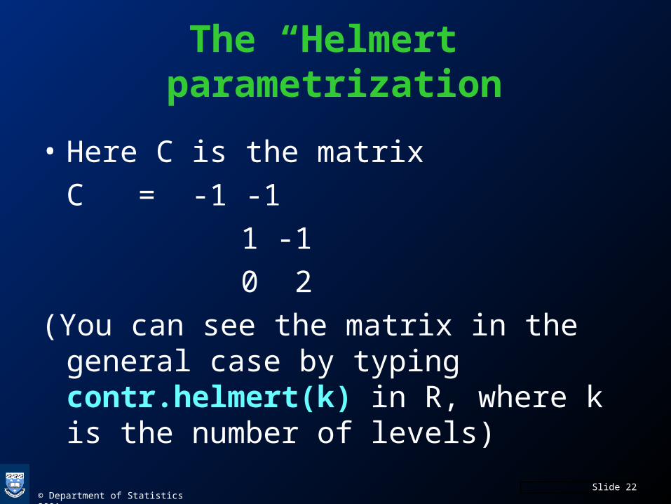
The “Helmert” parametrization
• Here C is the matrix
C = -1 -1
1 -1
0 2
(You can see the matrix in the general case by typing contr.helmert(k) in R, where k is the number of levels)

© Department of Statistics 2001Slide 23
Helmert parametrization (2)
• The model is E[Y] = Xwhere X is1 -1 -1
1 -1 -11 1 -1
1 1 -11 0 2
1 0 2• The effect of this reparametrization is to change all the rows and
columns.
. . .
. . .
. . .
. . .
Observations at level 1
Observations at level 2
Observations at level 3
© Department of Statistics 2001Slide 24
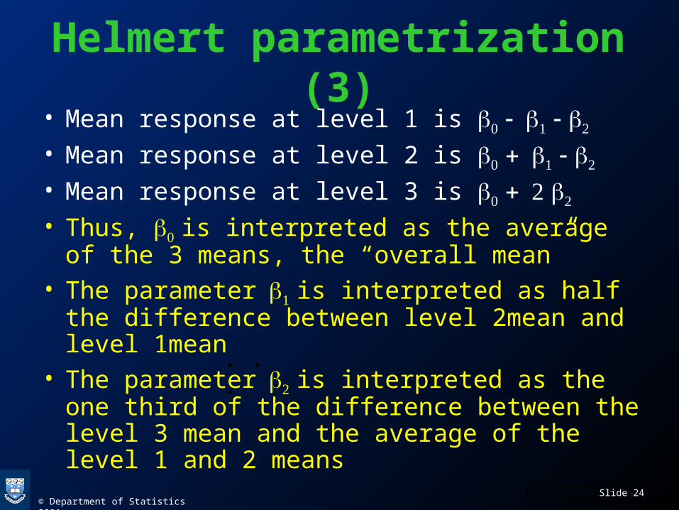
Helmert parametrization (3)
• Mean response at level 1 is
• Mean response at level 2 is
• Mean response at level 3 is
• Thus, is interpreted as the average of the 3 means, the “overall mean”
• The parameteris interpreted as half the difference between level 2mean and level 1mean
• The parameteris interpreted as the one third of the difference between the level 3 mean and the average of the level 1 and 2 means
. . .

© Department of Statistics 2001Slide 25
Using R to calculate the relationship between -parameters and means
TT
TT
XXX
XXX
X
1)(
Thus, the matrix (XTX)-1XT gives the coefficients we need to find the ’s from the ’s

© Department of Statistics 2001Slide 26
Example: One way model
• In an experiment to study the effect of carcinogenic substances, six different substances were applied to cell cultures.
• The response variable (ratio) is the ratio of damages to undamaged cells, and the explanatory variable (treatment) is the substance

© Department of Statistics 2001Slide 27
Dataratio treatment0.08 control + 49 other control obs0.08 choralhydrate + 49 other choralhydrate obs0.10 diazapan + 49 other diazapan obs0.10 hydroquinone + 49 other hydroquinine obs0.07 econidazole + 49 other econidazole obs0.17 colchicine + 49 other colchicine obs

© Department of Statistics 2001Slide 28
> cancer.lm<-lm(ratio ~ treatment,data=cancer.df)> summary(cancer.lm)Coefficients: Estimate Std. Error t value Pr(>|t|) (Intercept) 0.26900 0.02037 13.207 < 2e-16 ***treatmentcolchicine 0.17920 0.02881 6.221 1.69e-09 ***treatmentcontrol -0.03240 0.02881 -1.125 0.262 treatmentdiazapan 0.01180 0.02881 0.410 0.682 treatmenteconidazole -0.00420 0.02881 -0.146 0.884 treatmenthydroquinone 0.04300 0.02881 1.493 0.137 ---Signif. codes: 0 '***' 0.001 '**' 0.01 '*' 0.05 '.' 0.1 ' ' 1
Residual standard error: 0.144 on 294 degrees of freedomMultiple R-Squared: 0.1903, Adjusted R-squared: 0.1766 F-statistic: 13.82 on 5 and 294 DF, p-value: 3.897e-12
lm output

© Department of Statistics 2001Slide 29
Relationship between means and betas
X<-model.matrix(cancer.lm)coef.mat<-solve(t(X)%*%X)%*%t(X)
> levels(cancer.df$treatment)[1] "chloralhydrate" "colchicine" "control" "diazapan"
"econidazole" "hydroquinone"
> cancer.df$treatment[c(1,51,101,151,201,251)]control chloralhydrate diazapan hydroquinone econidazole
colchicine Levels: chloralhydrate colchicine control diazapan econidazole
hydroquinone> round(50*coef.mat[,c(1,51,101,151,201,251)]) 1 51 101 151 201 251(Intercept) 0 1 0 0 0 0treatmentcolchicine 0 -1 0 0 0 1treatmentcontrol 1 -1 0 0 0 0treatmentdiazapan 0 -1 1 0 0 0treatmenteconidazole 0 -1 0 0 1 0treatmenthydroquinone 0 -1 0 1 0 0

© Department of Statistics 2001Slide 30
Two factors: model y ~ a + b
To form X:
1. Start with column of 1’s
2. Add XaCa
3. Add XbCb

© Department of Statistics 2001Slide 31
Two factors: model y ~ a * b
To form X:
1. Start with column of 1’s
2. Add XaCa
3. Add XbCb
4. Add XaCa: XbCb
(Every column of XaCa multiplied elementwise with every column of XbCb)

© Department of Statistics 2001Slide 32
Two factors: example
Experiment to study weight gain in rats
– Response is weight gain over a fixed time period
– This is modelled as a function of diet (Beef, Cereal, Pork) and amount of feed (High, Low)
– See coursebook Section 4.4

© Department of Statistics 2001Slide 33
Data> diets.df gain source level1 73 Beef High2 98 Cereal High3 94 Pork High4 90 Beef Low5 107 Cereal Low6 49 Pork Low7 102 Beef High8 74 Cereal High9 79 Pork High10 76 Beef Low. . . 60 observations in all

© Department of Statistics 2001Slide 34
Two factors: the model
• If the (continuous) response depends on two categorical explanatory variables, then we assume that the response is normally distributed with a mean depending on the combination of factor levels: if the factors are A and B, the mean at the i th level of A and the j th level of B is ij
• Other standard assumptions (equal variance, normality, independence) apply

© Department of Statistics 2001Slide 35
Diagramatically…
Source = Beef
Source = Cereal
Source = Pork
Level=High
11 12 13
Level=Low
21 22 23

© Department of Statistics 2001Slide 36
Decomposition of the means
• We usually want to split each “cell mean” up into 4 terms:– A term reflecting the overall baseline level of
the response– A term reflecting the effect of factor A (row
effect)– A term reflecting the effect of factor B (column
effect)– A term reflecting how A and B interact.

© Department of Statistics 2001Slide 37
Mathematically…Overall Baseline: 11 (mean when both factors are at their baseline levels)
Effect of i th level of factor A (row effect): i111The i th level of A, at the baseline of B, expressed as a deviation from the overall baseline)
Effect of j th level of factor B (column effect) : 1j -11 (The j th level of B, at the baseline of A, expressed as a deviation from the overall baseline)Interaction: what’s left over (see next slide)

© Department of Statistics 2001Slide 38
Interactions• Each cell (except the first row and column) has
an interaction:Interaction = cell mean - baseline - row effect - column
effect
• If the interactions are all zero, then the effect of changing levels of A is the same for all levels of B – In mathematical terms, ij – i’j doesn’t depend on j
• Equivalently, effect of changing levels of B is the same for all levels of A
• If interactions are zero, relationship between factors and response is simple

© Department of Statistics 2001Slide 39
Splitting up the mean: rats
Cell Means
Beef Cereal Pork Baseline col
High 100 85.9 99.5 100
Low 79.2 83.9 78.7 79.2
Baseline row 100 85.9 99.5 100
Split-up
Beef Cereal Pork Row effect
High * * * *
Low * 18.8 0 -20.8
Col effect * -14.1 -0.5 100
Factors are : level (amount of food) and source (diet)
83.9 = 100 + (-20.8) + (-14.1) + 18.8
interaction

© Department of Statistics 2001Slide 40
Fit model> rats.lm<-lm(gain~source+level + source:level)> summary(rats.lm)
Coefficients: Estimate Std. Error t value Pr(>|t|) (Intercept) 1.000e+02 4.632e+00 21.589 < 2e-16 ***sourceCereal -1.410e+01 6.551e+00 -2.152 0.03585 * sourcePork -5.000e-01 6.551e+00 -0.076 0.93944 levelLow -2.080e+01 6.551e+00 -3.175 0.00247 ** sourceCereal:levelLow 1.880e+01 9.264e+00 2.029 0.04736 * sourcePork:levelLow -3.052e-14 9.264e+00 -3.29e-15 1.00000 ---Signif. codes: 0 `***' 0.001 `**' 0.01 `*' 0.05 `.' 0.1 ` ' 1
Residual standard error: 14.65 on 54 degrees of freedomMultiple R-Squared: 0.2848, Adjusted R-squared: 0.2185 F-statistic: 4.3 on 5 and 54 DF, p-value: 0.002299

© Department of Statistics 2001Slide 41
Fitting as a regression model
Note that using the treatment contrasts, this is equivalent to fitting a regression with dummy variables R2, C2, C3
R2 = 1 if obs is in row 2, zero otherwise
C2 = 1 if obs is in column 2, zero otherwise
C3 = 1 if obs is in column 3, zero otherwise
The regression is
Y ~ R2 + C2 + C3 + I(R2*C2) + I(R2*C3)

© Department of Statistics 2001Slide 42
NotationsFor two factors A and B
• Baseline: = 11
• A main effect: i = i1- 11
• B main effect: j = 1j - 11
• AB interaction: ij = ij - i1 - 1j + 11
• Then ij = + i + j + ij

© Department of Statistics 2001Slide 43
Re-label cell means, in data order
Source = Beef
Source = Cereal
Source = Pork
Level=High
1 2 3
Level=Low
4 5 6

© Department of Statistics 2001Slide 44
Using R to interpret parameters
>rats.df<-read.table(file.choose(), header=T)>rats.lm<-lm(gain~source*level, data=rats.df)>X<-model.matrix(rats.lm)>coef.mat<-solve(t(X)%*%X)%*%t(X)>round(10*coef.mat[,1:6]) 1 2 3 4 5 6(Intercept) 1 0 0 0 0 0sourceCereal -1 1 0 0 0 0sourcePork -1 0 1 0 0 0levelLow -1 0 0 1 0 0sourceCereal:levelLow 1 -1 0 -1 1 0sourcePork:levelLow 1 0 -1 -1 0 1
>rats.df[1:6,] gain source level1 73 Beef High2 98 Cereal High3 94 Pork High4 90 Beef Low5 107 Cereal Low6 49 Pork Low
Cell Means
betas

© Department of Statistics 2001Slide 45
X matrix: details (first six rows)
(Intercept) source source level sourceCereal: sourcePork: Cereal Pork Low levelLow levelLow
1 0 0 0 0 0
1 1 0 0 0 0
1 0 1 0 0 0
1 0 0 1 0 0
1 1 0 1 1 0
1 0 1 1 0 1
Col of 1’s XaCa XbCb XaCa:XbCb


