Statistics using ExcelTable 3: t-test assumin unequal variances 2.5 t-test for two samples assuming...

Statistics using Excel

Tsagris Michael

BSc in Statistics

Emai: [email protected]

mailto:[email protected]

Statistics Using Excel Tsagris Michael

2


Contents 1.1 Introduction............................................................................................................4 2.1 Data Analysis..........................................................................................................5 2.2 Descriptive Statistics..............................................................................................6 2.3 Z-test for two samples............................................................................................8 2.4 t-test for two samples assuming unequal variances ............................................9 2.5 t-test for two samples assuming equal variances ..............................................10 2.6 F-test for the equality of variances .....................................................................11 2.7 Paired t-test for two samples...............................................................................12 2.8 Ranks, Percentiles, Sampling, Random Numbers Generation........................13 2.9 Covariance, Correlation, Linear Regression.....................................................15 2.10 One-way Analysis of Variance..........................................................................18 2.11 Two-way Analysis of Variance with replication .............................................19 2.12 Two-way Analysis of Variance without replication........................................21 3.1 Statistical Functions.............................................................................................23 3.2 Spearman’s (non-parametric) correlation coefficient ......................................27 3.3 Wilcoxon Signed Rank Test for a Median.........................................................28 3.4 Wilcoxon Signed Rank Test with Paired Data ..................................................29

3


1.1 Introduction One of the reasons for which these notes were written was to help students and not only to perform some statistical analyses without having to use statistical software such as Splus, SPSS, and Minitab e.t.c. It is reasonable not to expect that excel offers much of the options for analyses offered by statistical packages but it is in a good level nonetheless. The areas covered by these notes are: descriptive statistics, z-test for two samples, t-test for two samples assuming (un)equal variances, paired t-test for two samples, F-test for the equality of variances of two samples, ranks and percentiles, sampling (random and periodic, or systematic), random numbers generation, Pearson’s correlation coefficient, covariance, linear regression, one-way ANOA, two-way ANOVA with and without replication and the moving average. We will also demonstrate the use of non-parametric statistics in Excel for some of the previously mentioned techniques. Furthermore, informal comparisons with the results provided by the Excel and the ones provided by SPSS and some other packages will be carried out to see for any discrepancies between Excel and SPSS. One thing that is worthy to mention before somebody goes through these notes is that they do not contain the theory underlying the techniques used. These notes show how to cope with statistics using Excel.

4


2.1 Data Analysis If the Excel does not offer you options for statistical analyses you can add this option very easily. Just click on the Add-Ins option in the list of Tools. In the dialog box (picture 2) appeared on the screen select the Analysis ToolPack. Excel will “run” this command for a couple of seconds and if select Tools you will see the option Data Analysis added on the list.

Picture 1

5


Picture 2

2.2 Descriptive Statistics The data used in most of the examples are taken from the SPSS file and refer to car measurements (cars.sav). We just copied and pasted the data in a worksheet of Excel. The road is always the same and mentioned already, tha is, by clicking Data Analysis in the list of Tools. The window of picture 3 appears on the screen. We Select Descriptive Statistics and click OK and we are lead to the window of picture 4. In the Input Range white box we specified the data, ranging from cell 1 to cell 406 all in one column. If the first row contained label we could just define it by clicking that option. We also clicked two of the last four options (Summary statistics, Confidence Level for Mean). As you can see the default value for the confidence level is 95%. In other words the confidence level is set to the usual 95%. The results produced by Excel are provided under the picture 3.

Picture 3

6


Picture 4

Column1 Mean 194.0418719 Standard Error 5.221297644 Median 148.5 Mode 97 Standard Deviation 105.2062324 Sample Variance 11068.35133 Kurtosis -0.79094723 Skewness 0.692125308 Range 451 Minimum 4 Maximum 455 Sum 78781 Count 406 Confidence Level(95.0%)

10.26422853

Table 1: Descriptive Statistics

The results are pretty much the same as should be. There are only some really slight differences with regard to the rounding in the results of SPSS but of not importance. The sample variances differ slightly but it is really not a problem. SPSS calculates a 95% confidence interval for the true mean whereas Excel provides only the quantity used to calculate the 95% confidence interval. The construction of this interval is really straightforward. Subtract this quantity from the mean to get the lower limit and add it to the mean to get the upper limit of the 95% confidence interval.

7


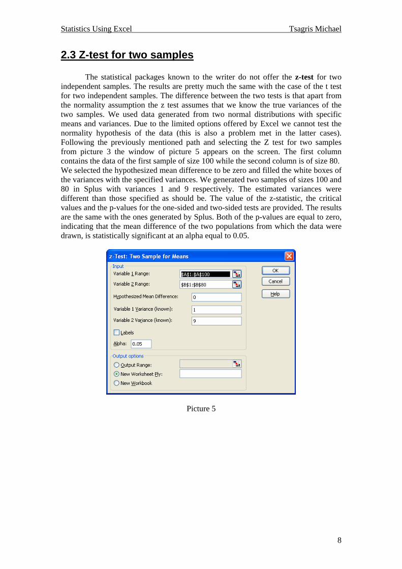
2.3 Z-test for two samples The statistical packages known to the writer do not offer the z-test for two independent samples. The results are pretty much the same with the case of the t test for two independent samples. The difference between the two tests is that apart from the normality assumption the z test assumes that we know the true variances of the two samples. We used data generated from two normal distributions with specific means and variances. Due to the limited options offered by Excel we cannot test the normality hypothesis of the data (this is also a problem met in the latter cases). Following the previously mentioned path and selecting the Z test for two samples from picture 3 the window of picture 5 appears on the screen. The first column contains the data of the first sample of size 100 while the second column is of size 80. We selected the hypothesized mean difference to be zero and filled the white boxes of the variances with the specified variances. We generated two samples of sizes 100 and 80 in Splus with variances 1 and 9 respectively. The estimated variances were different than those specified as should be. The value of the z-statistic, the critical values and the p-values for the one-sided and two-sided tests are provided. The results are the same with the ones generated by Splus. Both of the p-values are equal to zero, indicating that the mean difference of the two populations from which the data were drawn, is statistically significant at an alpha equal to 0.05.

Picture 5

8


z-Test: Two Sample for Means Variable 1 Variable 2

Mean 3.76501977 5.810701181 Known Variance 1 9 Observations 100 80 Hypothesized Mean Difference

0

z -5.84480403 P(Z<=z) one-tail 2.53582E-09 z Critical one-tail 1.644853627 P(Z<=z) two-tail 5.07165E-09 z Critical two-tail 1.959963985

Table 2: Z-test

2.4 t-test for two samples assuming unequal variances Theory states that when the variances of the two independent populations are not known (which is usually the case) we have to estimated them. The use of t-test is suggested in this case (but still the normality hypothesis has to be met unless the sample size is large). There are two approaches in this case; the one when we assume the variance to be equal and the one we cannot assume that. We will deal with the latter case now. We used the same data set as before since we know that the variances cannot be assumed to be equal. We will see the test of the equality of two variances later. Selecting the t-test assuming unequal variances from the window of picture 3 the window of picture 6 appears on the screen. The results generated from SPSS are the same except for some rounding differences.

Picture 6

9


t-Test: Two-Sample Assuming Unequal Variances

Variable 1 Variable 2 Mean 3.76501977 5.810701181 Variance 1.095786123 8.073733335 Observations 100 80 Hypothesized Mean Difference

0

df 96 t Stat -6.115932537 P(T<=t) one-tail 1.0348E-08 t Critical one-tail 1.660881441 P(T<=t) two-tail 2.06961E-08 t Critical two-tail 1.984984263

Table 3: t-test assumin unequal variances

2.5 t-test for two samples assuming equal variances We will perform the same test assuming that the equality of variances holds true. The window for this test following the famous path is that of picture 7.

Picture 7 The results are the same with the ones provided by SPSS. What is worthy to mention and to pay attention is that the degrees of freedom (df) for this case are equal to 178, whereas in the previous case were equal to 96. Also the t-statistics is slightly different. The reason it that different kind of formulae are used in both cases.

10


t-Test: Two-Sample Assuming Equal Variances

Variable 1 Variable 2 Mean 3.76501977 5.810701181 Variance 1.095786123 8.073733335 Observations 100 80 Pooled Variance 4.192740223 Hypothesized Mean Difference

0


Table 4: t-test assuming equal variances

2.6 F-test for the equality of variances We will now see how to test the hypothesis of the equality of variances. The window of picture 8 appears in the usual way by selecting the F-test from the window of picture 3. The results are the sam with the ones provided by Splus. The p-value is equal to zero indicating that there is evidence to reject the assumption of equality of the variance of the two samples at an alpha equal with 0.05.

Picture 8

11


F-Test Two-Sample for Variances Variable 1 Variable 2Mean 3.76501977 5.8107012Variance 1.09578612 8.0737333Observations 100 80 df 99 79 F 0.13572236 P(F<=f) one-tail

0

F Critical one-tail

0.70552977

Table 5: F-test for the equality of variances

2.7 Paired t-test for two samples Suppose that you are interested in testing the equality of two means, but the two samples (or the two populations) are not independent. For instance, when the data refer to the same people before and after a diet program. The window of picture 9 refers to this test. The results provided at table 6 are the same with the ones generated from SPSS. We can also see that the Pearson’s correlation coefficient is calculated.

Picture 9

12


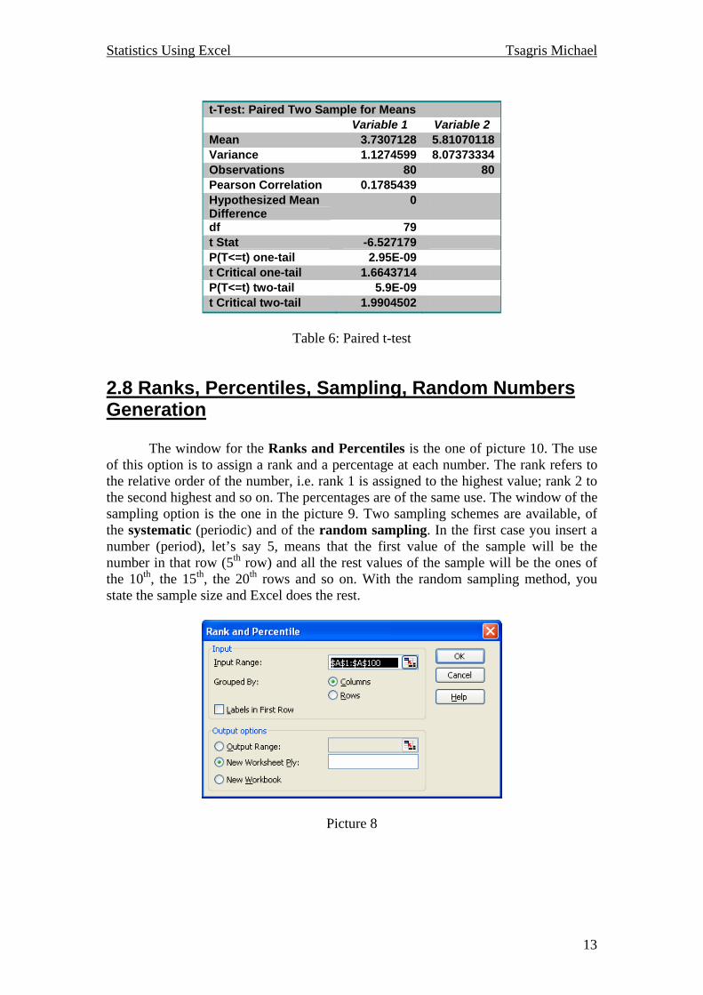
t-Test: Paired Two Sample for Means

Variable 1 Variable 2 Mean 3.7307128 5.81070118Variance 1.1274599 8.07373334Observations 80 80Pearson Correlation 0.1785439 Hypothesized Mean Difference

0


Table 6: Paired t-test

2.8 Ranks, Percentiles, Sampling, Random Numbers Generation The window for the Ranks and Percentiles is the one of picture 10. The use of this option is to assign a rank and a percentage at each number. The rank refers to the relative order of the number, i.e. rank 1 is assigned to the highest value; rank 2 to the second highest and so on. The percentages are of the same use. The window of the sampling option is the one in the picture 9. Two sampling schemes are available, of the systematic (periodic) and of the random sampling. In the first case you insert a number (period), let’s say 5, means that the first value of the sample will be the number in that row (5th row) and all the rest values of the sample will be the ones of the 10th, the 15th, the 20th rows and so on. With the random sampling method, you state the sample size and Excel does the rest.

Picture 8

13


Picture 9 If you are interested in a random sample from a know distribution then the random numbers generation is the option you want to use. Unfortunately not many distributions are offered. The window of this option is at picture 10. In the number of variables you can select how many samples you want to be drawn from the specific distribution. The white box below is used to define the sample size. The distributions offered are Uniform, Normal, Bernoulli, Binomial, and Poisson. Two more options are also allowed. Different distributions require different parameters to be defined. The random seed is an option used to give the sampling algorithm a starting value but can be left blank as well.

Picture 10

14


2.9 Covariance, Correlation, Linear Regression The covariance and correlation of two variables or two columns containing data is very easy to calculate. The windows of correlation and covariance are the same. We present the window of covariance.

Picture 11

Column 1

Column 2

Column 1

1.113367

Column 2

0.531949 7.972812

Table 7: Covariance

The above table is called the variance-covariance table since it produces both of these measures. The first cell (1.113367) refers to the variance of the first column and the last cell refers to the variance of the second column. The remaining cell (0.531949) refers to the covariance of the two columns. The blank cell is white due to the fact that the value is the covariance (the elements of the diagonal are the variances and the others refer to the covariance). The window of the linear regression option is presented at picture 12. (Different normal data used in the regression analysis). We fill the white boxes with the columns that represent Y and X values. The X values can contain more than one column (i.e. variable). We select the confidence interval option. We also select the Line Fit Plots and Normal Probability Plots. Then by pressing OK, the result appears in table 8.

15


Picture 12

SUMMARY OUTPUT Regression Statistics

Multiple R 0.875372 R Square 0.766276 Adjusted R Square

0.76328

Standard Error 23.06123 Observations 80 ANOVA

df SS MS F Significance F

Regression 1 136001 136001 255.7274 2.46E-26 Residual 78 41481.97 531.8202 Total 79 177483

Coefficients Standard Error

t Stat P-value Lower 95% Upper 95%

Intercept -10.6715 8.963642 -1.19053 0.237449 -28.5167 7.173767X Variable 1 0.043651 0.00273 15.99148 2.46E-26 0.038217 0.049085

Table 8: Analysis of variance table

The multiple R is the Pearson correlation coefficient, whereas the R Square is called coefficient of determination and it is a quantity that measures the fitting of the model. It shows the proportion of variability of the data explained by the linear model. The model is Y=-10.6715+0.043651*X. The adjusted R Square is the coefficient of determination adjusted for the degrees of freedom of the model; this is a penalty of the coefficient. The p-value of the constant provides evidence to claim that the constant is not statistical significant and therefore it should be removed from the model. So, if we run the regression again we will just click on Constant is Zero. The results are the same generated by SPSS except for some slight differences due to roundings. The disadvantage of Excel is that it offers no normality test. The two plots also constructed by Excel are presented.

16


X Variable 1 Line Fit Plot

0

50

100

150

200

250

0 2000 4000 6000

X Variable 1

Y YPredicted Y

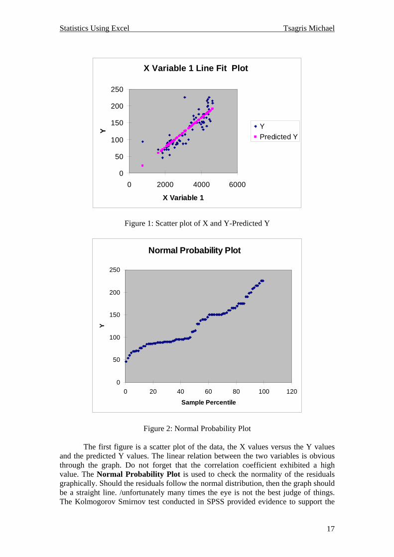
Figure 1: Scatter plot of X and Y-Predicted Y

Normal Probability Plot

0

50

100

150

200

250

0 20 40 60 80 100 120

Sample Percentile

Y

Figure 2: Normal Probability Plot The first figure is a scatter plot of the data, the X values versus the Y values and the predicted Y values. The linear relation between the two variables is obvious through the graph. Do not forget that the correlation coefficient exhibited a high value. The Normal Probability Plot is used to check the normality of the residuals graphically. Should the residuals follow the normal distribution, then the graph should be a straight line. /unfortunately many times the eye is not the best judge of things. The Kolmogorov Smirnov test conducted in SPSS provided evidence to support the

17


normality hypothesis of the residuals. Excel produced also the residuals and the predicted values in the same sheet. We shall construct a scatter plot of these two values, in order to check (graphically) the assumption of homoscedasticity (i.e. constant variance through the residuals). If the assumption of heteroscedasticity of the residuals holds true, then we should see all the values within a bandwidth. We see that almost all values fall within 40 and -40, except for two values that are over 70 and 100. These values are the so called outliers. We can assume that the residuals exhibit constant variance. If we are not certain as for the validity of the assumption we can transform the Y values using a log transformation and run the regression using the transformed Y values.

-60

-40

-20

0

20

40

60

80

100

120

0 50 100 150 200 250

Predicted Values

Res

idua

ls

Series1

Figure 3: Residuals versus predicted values

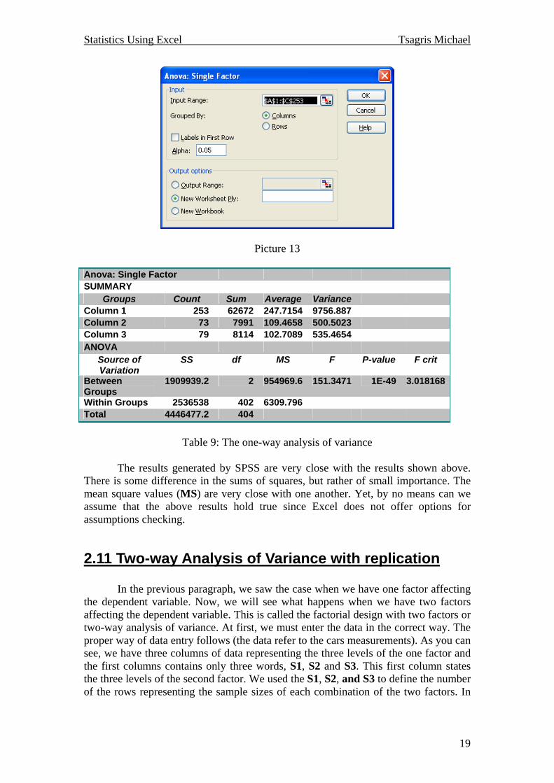
2.10 One-way Analysis of Variance The one-way analysis of variance is just the generalization of the two independent samples t-test. The assumptions the must be met in order for the results to be valid are more or less the same as in the linear regression case. It is a fact that analysis of variance and linear regression are two equivalent techniques. The Excel produces the analysis of variance table but offers no options to check the assumptions of the model. The window of the one way analysis of variance is shown at picture 13. As in the t-test cases the values of the independent variable are entered in Excel in different columns according to the factor. In our example we have three levels of the factor, therefore we have three columns. After defining the range of data in the window of picture 13, we click OK and the results follow.

18


Picture 13

Anova: Single Factor SUMMARY

Groups Count Sum Average Variance Column 1 253 62672 247.7154 9756.887 Column 2 73 7991 109.4658 500.5023 Column 3 79 8114 102.7089 535.4654 ANOVA

Source of Variation

SS df MS F P-value F crit

Between Groups

1909939.2 2 954969.6 151.3471 1E-49 3.018168

Within Groups 2536538 402 6309.796 Total 4446477.2 404

Table 9: The one-way analysis of variance

The results generated by SPSS are very close with the results shown above. There is some difference in the sums of squares, but rather of small importance. The mean square values (MS) are very close with one another. Yet, by no means can we assume that the above results hold true since Excel does not offer options for assumptions checking.

2.11 Two-way Analysis of Variance with replication In the previous paragraph, we saw the case when we have one factor affecting the dependent variable. Now, we will see what happens when we have two factors affecting the dependent variable. This is called the factorial design with two factors or two-way analysis of variance. At first, we must enter the data in the correct way. The proper way of data entry follows (the data refer to the cars measurements). As you can see, we have three columns of data representing the three levels of the one factor and the first columns contains only three words, S1, S2 and S3. This first column states the three levels of the second factor. We used the S1, S2, and S3 to define the number of the rows representing the sample sizes of each combination of the two factors. In

19


other words the first combination the two factors are the cells from B2 to B26. This means that each combination of factors has 24 measurements.

Picture 14 From the window of picture 3, we select Anova: Two-Factor with replication and the window to appear is shown at picture 15.

Picture 15 We filled the two blank white boxes with the input range and Rows per sample. The alpha is at its usual value, equal to 0.05. By pressing OK the results are presented overleaf. The results generated by SPSS are the same. At the bottom of the table 10 there are three p-values; two p-values for the two factors and one p-value for the interaction. The row factor is denoted as sample in Excel.

20


Anova: Two-Factor With Replication SUMMARY C1 C2 C3 Total

S1 Count 24 24 24 72 Sum 8229 2537 2378 13144 Average 342.875 105.7083 99.08333 182.5556 Variance 6668.288 237.5199 508.4275 15441.38



Total Count 72 72 72 Sum 21861 7894 7362 Average 303.625 109.6389 102.25 Variance 9660.181 505.3326 553.3732 ANOVA

Source of Variation


Sample (=Rows) 39713.18 2 19856.59 6.346116 0.002114 3.039508 Columns 1877690 2 938845.2 300.0526 6.85E-62 3.039508 Interaction 73638.1 4 18409.53 5.883638 0.000167 2.415267 Within 647689.7 207 3128.936 Total 2638731 215

Table 10: The two-way analysis of variance with replication

2.12 Two-way Analysis of Variance without replication We will now see another case of the two-way ANOVA when each combination of factors has only one measurement. In this case we need not enter the data as in the previous case in which the labels were necessary. We will use only the three first three rows of the data. We still have two factors except for the fact that each combination contains one measurement. From the window of picture 3, we select Anova: Two-Factor without replication and the window to appear is shown at picture 16. The only thing we did was to define the Input Range and pressed OK. The results are presented under picture 16. What is necessary for this analysis is that there no interaction is present. The results are the same with the ones provided by SPSS, so we conclude once again that Excel works fine with statistical analysis. The disadvantage of Excel is once again that it provides no formulas for examining the residuals in the case of analysis of variance.

21


Picture 16

Anova: Two-Factor Without Replication

SUMMARY Count Sum Average Variance Row 1 3 553 184.3333 11385.33 Row 2 3 544 181.3333 21336.33 Row 3 3 525 175 15379 Column 1 3 975 325 499 Column 2 3 340 113.3333 332.3333 Column 3 3 307 102.3333 85.33333 ANOVA

Source of Variation


Rows 136.2222 2 68.11111 0.160534 0.856915 6.944272 Columns 94504.22 2 47252.11 111.3707 0.000311 6.944272 Error 1697.111 4 424.2778 Total 96337.56 8

Table 11: The two-way analysis of variance without replication

22


3.1 Statistical Functions Before showing how to find statistical measures using the statistical functions available from Excel under the Insert Function option let us see which are these.

• AVEDEV calculates the average of the absolute deviations of the data from their mean.

• AVERAGE is the mean value of all data points. • AVERAGEA calculates the mean allowing for text values of FALSE

(evaluated as 0) and TRUE (evaluated as 1). • BETADIST calculates the cumulative beta probability density function. • BETAINV calculates the inverse of the cumulative beta probability density

function. • BINOMDIST determines the probability that a set number of true/false trials,

where each trial has a consistent chance of generating a true or false result, will result in exactly a specified number of successes (for example, the probability that exactly four out of eight coin flips will end up heads).

• CHIDIST calculates the one-tailed probability of the chi-squared distribution.

• CHIINV calculates the inverse of the one-tailed probability of the chi-squared.

Distribution.

• CHITEST calculates the result of the test for independence: the value from the chi-squared distribution for the statistics and the appropriate degrees of freedom.

• CONFIDENCE returns a value you can use to construct a confidence interval

for a population mean.

• CORREL returns the correlation coefficient between two data sets.

• COVAR calculates the covariance of two data sets. Mathematically, it is the multiplication of the correlation coefficient with the standard deviations of the two data sets.

• CRITBINOM determines when the number of failures in a series of true/false

trials exceeds a criterion (for example, more than 5 percent of light bulbs in a production run fail to light).

• DEVSQ calculates the sum of squares of deviations of data points from their

sample mean. The derivation of standard deviation is very straightforward, simply dividing by the sample size or by the sample size decreased by one to get the unbiased estimator of the true standard deviation.

23


• EXPODIST returns the exponential distribution

• FDIST calculates the F probability distribution (degree of diversity) for two data sets.

• FINV returns the inverse of the F probability distribution.

• FISHER calculates the Fisher transformation.

• FISHERINV returns the inverse of the Fisher transformation.

• FORECAST calculates a future value along a linear trend based on an existing

time series of values.

• FREQUENCY calculates how often values occur within a range of values and then returns a vertical array of numbers having one or more elements than Bins_array.

• FTEST returns the result of the one-tailed test that the variances of two data

sets are not significantly different.

• GAMMADIST calculates the gamma distribution.

• GAMMAINV returns the inverse of the gamma distribution.

• GAMMALN calculates the natural logarithm of the gamma distribution.

• GEOMEAN calculates the geometric mean.

• GROWTH predicts the exponential growth of a data series.

• HARMEAN calculates the harmonic mean.

• HYPGEOMDIST returns the probability of selecting an exact number of a single type of item from a mixed set of objects. For example, a jar holds 20 marbles, 6 of which are red. If you choose three marbles, what is the probability you will pick exactly one red marble?

• INTERCEPT calculates the point at which a line will intersect the y-axis.

• KURT calculates the kurtosis of a data set.

• LARGE returns the k-th largest value in a data set. • LINEST generates a line that best fits a data set by generating a two

dimensional array of values to describe the line.

• LOGEST generates a curve that best fits a data set by generating a two dimensional array of values to describe the curve.

24


• LOGINV returns the inverse logarithm of a value in a distribution.

• LOGNORMDIST Returns the number of standard deviations a value is away

from the mean in a lognormal distribution.

• MAX returns the largest value in a data set (ignore logical values and text).

• MAXA returns the largest value in a set of data (does not ignore logical values and text).

• MEDIAN returns the median of a data set.

• MIN returns the largest value in a data set (ignore logical values and text).

• MINA returns the largest value in a data set (does not ignore logical values

and text).

• MODE returns the most frequently occurring values in an array or range of data.

• NEGBINOMDIST returns the probability that there will be a given number of

failures before a given number of successes in a binomial distribution. • NORMDIST returns the number of standard deviations a value is away from

the mean in a normal distribution.

• NORMINV returns a value that reflects the probability a random value selected from a distribution will be above it in the distribution.

• NORMSDIST returns a standard normal distribution, with a mean of 0 and a

standard deviation of 1.

• NORMSINV returns a value that reflects the probability a random value selected from the standard normal distribution will be above it in the distribution.

• PEARSON returns a value that reflects the strength of the linear relationship

between two data sets.

• PERCENTILE returns the k-th percentile of values in a range.

• PERCENTRANK returns the rank of a value in a data set as a percentage of the data set.

• PERMUT calculates the number of permutations for a given number of

objects that can be selected from the total objects.

25


• POISSON returns the probability of a number of events happening, given the Poisson distribution of events.

• PROB calculates the probability that values in a range are between two limits

or equal to a lower limit.

• QUARTILE returns the quartile of a data set.

• RANK calculates the rank of a number in a list of numbers: its size relative to other values in the list.

• RSQ calculates the square of the Pearson correlation coefficient (also met as

coefficient of determination in the case of linear regression).

• SKEW returns the skewness of a data set (the degree of asymmetry of a distribution around its mean).

• SLOPE returns the slope of a line.

• SMALL returns the k-th smallest values in a data set.

• STANDARDIZE calculates the normalized values of a data set (each value

minus the mean and then divided by the standard deviation). • STDEV estimates the standard deviation of a numerical data set based on a

sample of the data.

• STDEVA estimates the standard deviation of a data set (which can include text and true/false values) based on a sample of the data.

• STDEVP calculates the standard deviation of a numerical data set.

• STDEVPA calculates the standard deviation of a data set (which can include

text and true/false values).

• STEYX returns the predicted standard error for the y value for each x value in regression.

• TDIST returns the Student’s t distribution

• TINV returns a t value based on a stated probability and degrees of freedom.

• TREND Returns values along a trend line.

• TRIMMEAN calculates the mean of a data set having excluded a percentage

of the upper and lower values.

• TTEST returns the probability associated with a Student’s t distribution.

26


• VAR estimates the variance of a data sample.

• VARA estimates the variance of a data set (which can include text and true/ false values) based on a sample of the data.

• VARP calculates the variance of a data population.

• VARPA calculates the variance of a data population, which can include text

and true/false values.

• WEIBULL calculates the Weibull distribution.

• ZTEST returns the two-tailed p-value of a z-test.

3.2 Spearman’s (non-parametric) correlation coefficient The Spearman’s correlation coefficient is the non-parametric alternative of the Pearson’s correlation coefficient. It is the Pearson’s correlation coefficient based upon the ranks of the values rather than the values. In paragraph 2.8 we exhibited how to calculate the ranks for a range of values. The selection of calculation of the ranks will generate this in Excel:

Point Column1 Rank Percent 55 183 1 100.00%43 168 2 98.50%50 163 3 95.70%52 163 3 95.70%63 146 5 94.30%71 145 6 92.90%56 141 7 90.10%69 141 7 90.10%

1 133 9 88.70%49 131 10 87.30%41 130 11 85.90%66 122 12 84.50%

6 121 13 69.00%13 121 13 69.00%14 121 13 69.00%22 121 13 69.00%23 121 13 69.00%34 121 13 69.00%35 121 13 69.00%47 121 13 69.00%

Table 12: Ranks and Percentiles

27


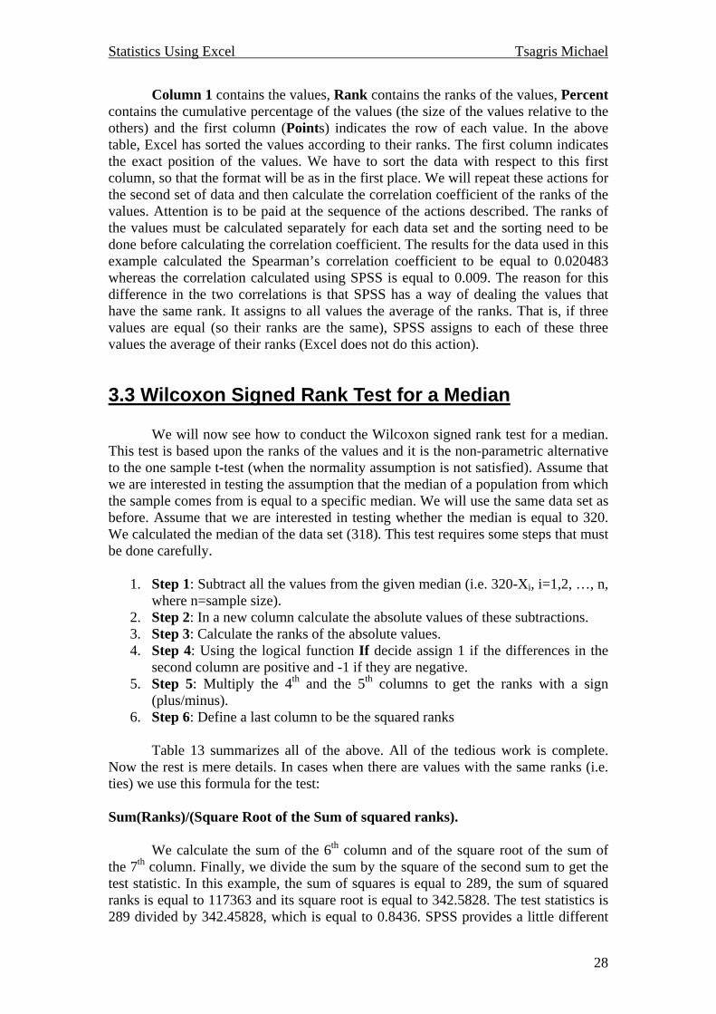
Column 1 contains the values, Rank contains the ranks of the values, Percent contains the cumulative percentage of the values (the size of the values relative to the others) and the first column (Points) indicates the row of each value. In the above table, Excel has sorted the values according to their ranks. The first column indicates the exact position of the values. We have to sort the data with respect to this first column, so that the format will be as in the first place. We will repeat these actions for the second set of data and then calculate the correlation coefficient of the ranks of the values. Attention is to be paid at the sequence of the actions described. The ranks of the values must be calculated separately for each data set and the sorting need to be done before calculating the correlation coefficient. The results for the data used in this example calculated the Spearman’s correlation coefficient to be equal to 0.020483 whereas the correlation calculated using SPSS is equal to 0.009. The reason for this difference in the two correlations is that SPSS has a way of dealing the values that have the same rank. It assigns to all values the average of the ranks. That is, if three values are equal (so their ranks are the same), SPSS assigns to each of these three values the average of their ranks (Excel does not do this action).

3.3 Wilcoxon Signed Rank Test for a Median We will now see how to conduct the Wilcoxon signed rank test for a median. This test is based upon the ranks of the values and it is the non-parametric alternative to the one sample t-test (when the normality assumption is not satisfied). Assume that we are interested in testing the assumption that the median of a population from which the sample comes from is equal to a specific median. We will use the same data set as before. Assume that we are interested in testing whether the median is equal to 320. We calculated the median of the data set (318). This test requires some steps that must be done carefully.

1. Step 1: Subtract all the values from the given median (i.e. 320-Xi, i=1,2, …, n, where n=sample size).

2. Step 2: In a new column calculate the absolute values of these subtractions. 3. Step 3: Calculate the ranks of the absolute values. 4. Step 4: Using the logical function If decide assign 1 if the differences in the

second column are positive and -1 if they are negative. 5. Step 5: Multiply the 4th and the 5th columns to get the ranks with a sign

(plus/minus). 6. Step 6: Define a last column to be the squared ranks

Table 13 summarizes all of the above. All of the tedious work is complete. Now the rest is mere details. In cases when there are values with the same ranks (i.e. ties) we use this formula for the test: Sum(Ranks)/(Square Root of the Sum of squared ranks). We calculate the sum of the 6th column and of the square root of the sum of the 7th column. Finally, we divide the sum by the square of the second sum to get the test statistic. In this example, the sum of squares is equal to 289, the sum of squared ranks is equal to 117363 and its square root is equal to 342.5828. The test statistics is 289 divided by 342.45828, which is equal to 0.8436. SPSS provides a little different

28


test statistics due to the different handling of the tied ranks and the use of different test statistic. There is also another way to calculate a test statistics and that is by taking the sum of the positive ranks. Both Minitab and SPSS calculate another type of test statistic, which is based on either the positive or the negative ranks. What is worthy to mention is that the second formula is better used in the case when there are no tied ranks. Irrespectively of the test statistics used the result will be the same as for the rejection of the null hypothesis. Using the second formula the result is 1401, whereas Minitab provides a result of 1231.5. As for the result of the test (reject the null hypothesis or not) one must look at the tables for the 1 sample Wilcoxon signed rank test. The fact that Excel does not offer options for calculating the probabilities used in the non-parametric tests in conjunction with the tedious work, makes it less popular for use. Values (Xi)

m-Xi absolute(m-Xi)

Ranks of absolute values

positive or negative differences

Ranks Ri

Squared Ranks Ri

2

307 13 13 64 1 64 4096350 -30 30 47 -1 -47 2209318 2 2 67 1 67 4489304 16 16 60 1 60 3600302 18 18 56 1 56 3136429 -109 109 19 -1 -19 361454 -134 134 13 -1 -13 169440 -120 120 17 -1 -17 289455 -135 135 11 -1 -11 121390 -70 70 32 -1 -32 1024350 -30 30 47 -1 -47 2209351 -31 31 43 -1 -43 1849383 -63 63 37 -1 -37 1369360 -40 40 41 -1 -41 1681383 -63 63 37 -1 -37 1369

Table 13: Procedure of the Wilcoxon Signed Rank Test

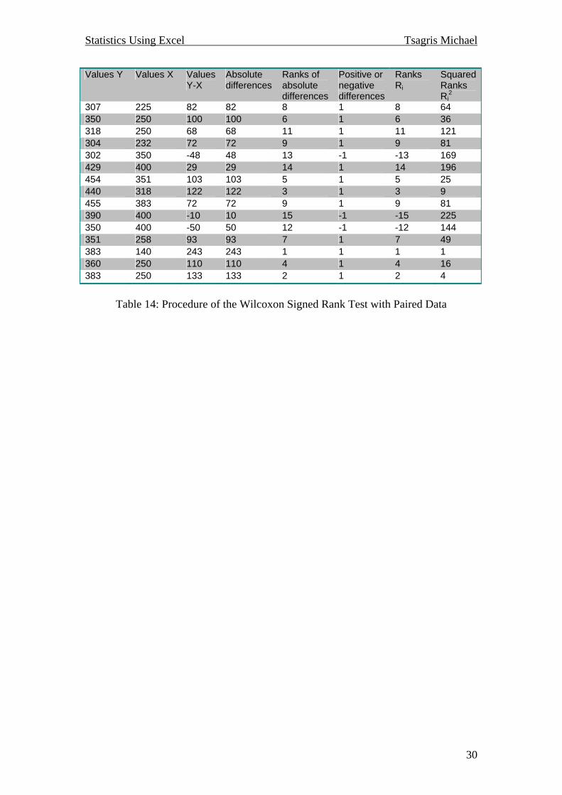
3.4 Wilcoxon Signed Rank Test with Paired Data When we have two samples which cannot be assumed to be independent (i.e. the weight of people before and after a diet) and we are interested in testing the hypothesis that the two medians are equal versus they are not then the use of the Wilcoxon signed rank test with paired data is necessary. This is the non-parametric alternative to the paired samples t-test. The procedure is the same with the one sample case. We will only have to add another column representing the values of the second sample, so the table 13 would have 8 columns instead of 7 and the third column would be the differences between the values of the two data sets. The formulae for the test statistics are the same as before and the results will be different from SPSS due to the fact that Excel (in contrast to SPSS) does not manipulate ties in the ranks. The tables of the critical values for this test must be available in order to decide whether to reject or not the null hypothesis.

29


Values Y Values X Values Y-X

Absolute differences

Ranks of absolute differences

Positive or negative differences

Ranks Ri

Squared Ranks Ri

2

307 225 82 82 8 1 8 64 350 250 100 100 6 1 6 36 318 250 68 68 11 1 11 121 304 232 72 72 9 1 9 81 302 350 -48 48 13 -1 -13 169 429 400 29 29 14 1 14 196 454 351 103 103 5 1 5 25 440 318 122 122 3 1 3 9 455 383 72 72 9 1 9 81 390 400 -10 10 15 -1 -15 225 350 400 -50 50 12 -1 -12 144 351 258 93 93 7 1 7 49 383 140 243 243 1 1 1 1 360 250 110 110 4 1 4 16 383 250 133 133 2 1 2 4

Table 14: Procedure of the Wilcoxon Signed Rank Test with Paired Data

30

Statistics using ExcelTable 3: t-test assumin unequal variances 2.5 t-test for two samples assuming...

Documents

Transcript of Statistics using ExcelTable 3: t-test assumin unequal variances 2.5 t-test for two samples assuming...