This article was downloaded by: [University of Minnesota Libraries, Twin Cities]On: 24 July 2013, At: 11:35Publisher: Taylor & FrancisInforma Ltd Registered in England and Wales Registered Number: 1072954 Registeredoffice: Mortimer House, 37-41 Mortimer Street, London W1T 3JH, UK

Journal of Computational and GraphicalStatisticsPublication details, including instructions for authors andsubscription information:http://www.tandfonline.com/loi/ucgs20

An Efficient Algorithm for Computing theHHSVM and Its GeneralizationsYi Yang a & Hui Zou aa University of Minnesota , Minneapolis , MN , 55455-0213Accepted author version posted online: 25 Apr 2012.Publishedonline: 30 May 2013.

To cite this article: Yi Yang & Hui Zou (2013) An Efficient Algorithm for Computing the HHSVMand Its Generalizations, Journal of Computational and Graphical Statistics, 22:2, 396-415, DOI:10.1080/10618600.2012.680324

To link to this article: http://dx.doi.org/10.1080/10618600.2012.680324

PLEASE SCROLL DOWN FOR ARTICLE

Taylor & Francis makes every effort to ensure the accuracy of all the information (the“Content”) contained in the publications on our platform. However, Taylor & Francis,our agents, and our licensors make no representations or warranties whatsoever as tothe accuracy, completeness, or suitability for any purpose of the Content. Any opinionsand views expressed in this publication are the opinions and views of the authors,and are not the views of or endorsed by Taylor & Francis. The accuracy of the Contentshould not be relied upon and should be independently verified with primary sourcesof information. Taylor and Francis shall not be liable for any losses, actions, claims,proceedings, demands, costs, expenses, damages, and other liabilities whatsoever orhowsoever caused arising directly or indirectly in connection with, in relation to or arisingout of the use of the Content.

This article may be used for research, teaching, and private study purposes. Anysubstantial or systematic reproduction, redistribution, reselling, loan, sub-licensing,systematic supply, or distribution in any form to anyone is expressly forbidden. Terms &Conditions of access and use can be found at http://www.tandfonline.com/page/terms-and-conditions

Supplementary materials for this article are available online.Please go to www.tandfonline.com/r/JCGS

An Efficient Algorithm for Computing theHHSVM and Its Generalizations

Yi YANG and Hui ZOU

The hybrid Huberized support vector machine (HHSVM) has proved its advantagesover the �1 support vector machine (SVM) in terms of classification and variable selec-tion. Similar to the �1 SVM, the HHSVM enjoys a piecewise linear path property andcan be computed by a least-angle regression (LARS)-type piecewise linear solution pathalgorithm. In this article, we propose a generalized coordinate descent (GCD) algorithmfor computing the solution path of the HHSVM. The GCD algorithm takes advantageof a majorization–minimization trick to make each coordinatewise update simple andefficient. Extensive numerical experiments show that the GCD algorithm is much fasterthan the LARS-type path algorithm. We further extend the GCD algorithm to solve aclass of elastic net penalized large margin classifiers, demonstrating the generality ofthe GCD algorithm. We have implemented the GCD algorithm in a publicly availableR package gcdnet.

Key Words: Coordinate descent; Elastic net; Hubernet; Large margin classifiers;Majorization–minimization; SVM.

1. INTRODUCTION

The support vector machine (SVM; Vapnik 1995) is a very popular large margin classifier.Despite its competitive performance in terms of classification accuracy, a major limitation ofthe SVM is that it cannot automatically select relevant variables for classification, which isvery important in high-dimensional classification problems such as tumor classification withmicroarrays. The SVM has an equivalent formulation as the �2 penalized hinge loss (Hastie,Tibshirani, and Friedman 2001). Bradley and Mangasarian (1998) proposed the �1 SVMby replacing the �2 penalty in the SVM with the �1 penalty. The �1 penalization (aka lasso)(Tibshirani 1996) is a very popular technique for achieving sparsity with high-dimensionaldata. There has been a large body of theoretical work to support the �1 regularization. Acomprehensive reference is Buhlmann and van de Geer (2011). Wang, Zhu, and Zou (2008)later proposed a hybrid Huberized support vector machine (HHSVM) that uses the elastic

Yi Yang (E-mail: yiyang@umn.edu) is Ph.D. student and Hui Zou (E-mail: zouxx019@umn.edu) is AssociateProfessor in School of Statistics at University of Minnesota, Minneapolis, MN 55455-0213.

C© 2013 American Statistical Association, Institute of Mathematical Statistics,and Interface Foundation of North America

Journal of Computational and Graphical Statistics, Volume 22, Number 2, Pages 396–415DOI: 10.1080/10618600.2012.680324

396

Dow

nloa

ded

by [

Uni

vers

ity o

f M

inne

sota

Lib

rari

es, T

win

Citi

es]

at 1

1:35

24

July

201

3

AN ALGORITHM FOR COMPUTING THE HHSVM 397

net penalty (Zou and Hastie 2005) for regularization and variable selection and uses theHuberized squared hinge loss for efficient computation. Wang, Zhu, and Zou (2008) showedthat the HHSVM outperforms the standard SVM and the �1 SVM for high-dimensionalclassification. Wang, Zhu, and Zou (2008) extended the least-angle regression (LARS)algorithm for the lasso regression model (Osborne, Presnell, and Turlach 2000; Efron et al.2004, Rosset and Zhu 2007) to compute the solution paths of the HHSVM.

The main purpose of this article is to introduce a new efficient algorithm for computingthe HHSVM. Our study was motivated by the recent success of using coordinate descentalgorithms for computing the elastic net penalized regression and logistic regression (Fried-man, Hastie, and Tibshirani 2010; see also Van der Kooij 2007). For the lasso regression,the coordinate descent algorithm amounts to an iterative cyclic soft-thresholding operation.Despite its simplicity, the coordinate descent algorithm can even outperform the LARSalgorithm, especially when the dimension is much larger than the sample size (see table1 of Friedman, Hastie, and Tibshirani 2010). Other articles on coordinate descent algo-rithms for the lasso include Fu (1998), Daubechies, Defrise, and De Mol (2004), Friedmanet al. (2007), Genkin, Lewis, and Madigan (2007), Wu and Lange (2008), and amongothers. The HHSVM poses a major challenge for applying the coordinate descent algo-rithm, because the Huberized hinge loss function does not have a smooth first derivativeeverywhere. As a result, the coordinate descent algorithm for the elastic net penalizedlogistic regression (Friedman, Hastie, and Tibshirani 2010) cannot be used for solving theHHSVM.

To overcome the computational difficulty, we propose a new generalized coordinatedescent (GCD) algorithm for solving the solution paths of the HHSVM. We also give afurther extension of the GCD algorithm to general problems. Our algorithm adopts themajorization–minimization (MM) principle into the coordinate descent loop. We use anMM trick to make each coordinatewise update simple and efficient. In addition, the MMprinciple ensures the descent property of the GCD algorithm which is crucial for all co-ordinate descent algorithms. Extensive numerical examples show that the GCD can bemuch faster than the LARS-type path algorithm in Wang, Zhu, and Zou (2008). Here weuse the prostate cancer data (Singh et al. 2002) to briefly illustrate the speed advantageof our algorithm (see Figure 1). The prostate data have 102 observations and each has6033 gene expression values. It took the LARS-type path algorithm about 5 min to com-pute the HHSVM paths, while the GCD used only 3.5 sec to get the identical solutionpaths.

A closer examination of the GCD algorithm reveals that it can be used for solving otherlarge margin classifiers. We have derived a generic GCD algorithm for solving a class ofelastic net penalized large margin classifiers. We further demonstrate the generic GCDalgorithm by considering the squared SVM loss and the logistic regression loss. We studythrough numeric examples how the shape and smoothness of the loss function affect thecomputational speed of the generic GCD algorithm.

In Section 2, we review the HHSVM and then introduce the GCD algorithm for comput-ing the HHSVM. Section 3 studies the descent property of the GCD algorithm by makingan intimate connection to the MM principle. The analysis motivates us to further consider ageneric GCD algorithm for handling a class of elastic net penalized large margin classifiers.Numerical experiments are presented in Section 5.

Dow

nloa

ded

by [

Uni

vers

ity o

f M

inne

sota

Lib

rari

es, T

win

Citi

es]

at 1

1:35

24

July

201

3

398 Y. YANG AND H. ZOU

Figure 1. Solution paths and timings of the HHSVM on the prostate cancer data with 102 observations and 6033predictors. The top panel shows the solution paths computed by the LARS-type algorithm in Wang, Zhu, and Zou(2008); the bottom panel shows the solution paths computed by GCD. GCD is 87 times faster.

Dow

nloa

ded

by [

Uni

vers

ity o

f M

inne

sota

Lib

rari

es, T

win

Citi

es]

at 1

1:35

24

July

201

3

AN ALGORITHM FOR COMPUTING THE HHSVM 399

2. THE HHSVM AND GCD ALGORITHM

2.1 THE HHSVM

In a standard binary classification problem, we are given n pairs of training data{xi , yi} for i = 1, . . . , n where xi ∈ Rp are predictors and yi ∈ {−1, 1} denotes class labels.The linear SVM (Vapnik 1995; Burges 1998; Evgeniou, Pontil, and Poggio 2000) looks forthe hyperplane with the largest margin that separates the input data for class 1 and class −1

min(β0,β)

1

2||β||2 + γ

n∑i=1

ξi

subject to ξi ≥ 0, yi

(β0 + xᵀ

i β) ≥ 1 − ξi ∀i, (2.1)

where ξ = (ξ1, ξ2, . . . , ξn) are the slack variables and γ > 0 is a constant. Let λ = 1/(nγ ).Then (2.1) has an equivalent �2 penalized hinge loss formulation (Hastie, Tibshirani, andFriedman 2001)

min(β0,β)

1

n

n∑i=1

[1 − yi

(β0 + xᵀ

i β)]

+ + λ

2||β||22. (2.2)

The loss function L(t) = [1 − t]+ has the expression

[1 − t]+ ={

0,

1 − t,

t > 1t ≤ 1,

which is called the hinge loss in the literature. The SVM has very competitive performancein terms of classification. However, because of the �2 penalty the SVM uses all variables inclassification, which could be a great disadvantage in high-dimensional classification (Zhuet al. 2004). The �1 SVM proposed by Bradley and Mangasarian (1998) is defined by

min(β0,β)

1

n

n∑i=1

[1 − yi

(β0 + xᵀ

i β)]

+ + λ

2||β||1. (2.3)

Just like in the lasso regression model, the �1 penalty produces a sparse β in (2.3). Thus the�1 SVM is able to automatically discard irrelevant features. In the presence of many noisevariables, the �1 SVM has significant advantages over the standard SVM (Zhu et al. 2004).

The elastic net penalty (Zou and Hastie 2005) is an important generalization of the lassopenalty. The elastic net penalty is defined as

Pλ1,λ2 (β) =p∑

j=1

pλ1,λ2 (βj ) =p∑

j=1

(λ1|βj | + λ2

2β2

j

), (2.4)

where λ1, λ2 ≥ 0 are regularization parameters. The �1 part of the elastic net is responsiblefor variable selection. The �2 part of the elastic net helps handle strong correlated variables,which is common in high-dimensional data, and improves prediction.

Wang, Zhu, and Zou (2008) used the elastic net in the SVM classification:

min(β0,β)

1

n

n∑i=1

φc

(yi

(β0 + xᵀ

i β)) + Pλ1,λ2 (β). (2.5)

Dow

nloa

ded

by [

Uni

vers

ity o

f M

inne

sota

Lib

rari

es, T

win

Citi

es]

at 1

1:35

24

July

201

3

400 Y. YANG AND H. ZOU

Figure 2. (a) The Huberized hinge loss function (with δ = 2); (b) the Huberized hinge loss function (withδ = 0.01); (c) the squared hinge loss function; (d) the logistic loss function.

Note that φc(·) in (2.5) is the Huberized hinge loss

φc(t) =⎧⎨⎩

0,

(1 − t)2/2δ,

1 − t − δ/2,

t > 11 − δ < t ≤ 1t ≤ 1 − δ,

where δ > 0 is a pre-specified constant. The default choice for δ is 2 unless specified other-wise. Displayed in Figure 2 panel (a) is the Huberized hinge loss with δ = 2. The Huberizedhinge loss is very similar to the hinge loss in shape. In fact, when δ is small, the two loss func-tions are almost identical. See Figure 2 panel (b) for a graphical illustration. Unlike the hingeloss, the Huberized hinge loss function is differentiable everywhere and has continuous firstderivative. Wang, Zhu, and Zou (2008) derived a LARS-type path algorithm for comput-ing the solution paths of the HHSVM. Compared with the LARS-type algorithm for the�1 SVM (Zhu et al. 2004), the LARS-type algorithm for the HHSVM has significantly lowercomputational cost, thanks to the differentiability property of the Huberized hinge loss.

Dow

nloa

ded

by [

Uni

vers

ity o

f M

inne

sota

Lib

rari

es, T

win

Citi

es]

at 1

1:35

24

July

201

3

AN ALGORITHM FOR COMPUTING THE HHSVM 401

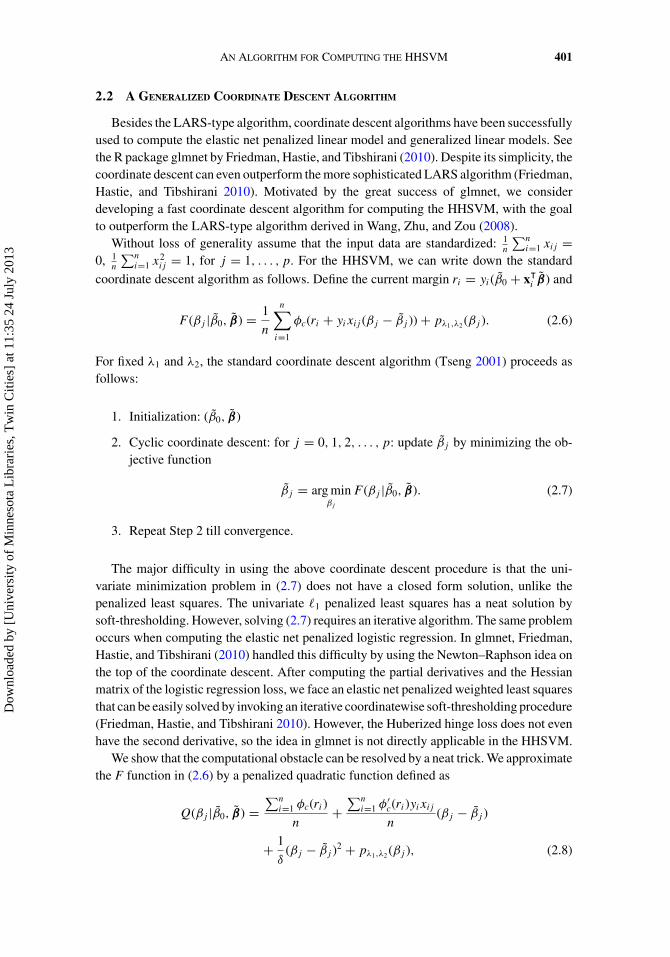
2.2 A GENERALIZED COORDINATE DESCENT ALGORITHM

Besides the LARS-type algorithm, coordinate descent algorithms have been successfullyused to compute the elastic net penalized linear model and generalized linear models. Seethe R package glmnet by Friedman, Hastie, and Tibshirani (2010). Despite its simplicity, thecoordinate descent can even outperform the more sophisticated LARS algorithm (Friedman,Hastie, and Tibshirani 2010). Motivated by the great success of glmnet, we considerdeveloping a fast coordinate descent algorithm for computing the HHSVM, with the goalto outperform the LARS-type algorithm derived in Wang, Zhu, and Zou (2008).

Without loss of generality assume that the input data are standardized: 1n

∑ni=1 xij =

0, 1n

∑ni=1 x2

ij = 1, for j = 1, . . . , p. For the HHSVM, we can write down the standard

coordinate descent algorithm as follows. Define the current margin ri = yi(β0 + xᵀi β) and

F (βj |β0, β) = 1

n

n∑i=1

φc(ri + yixij (βj − βj )) + pλ1,λ2 (βj ). (2.6)

For fixed λ1 and λ2, the standard coordinate descent algorithm (Tseng 2001) proceeds asfollows:

1. Initialization: (β0, β)

2. Cyclic coordinate descent: for j = 0, 1, 2, . . . , p: update βj by minimizing the ob-jective function

βj = arg minβj

F (βj |β0, β). (2.7)

3. Repeat Step 2 till convergence.

The major difficulty in using the above coordinate descent procedure is that the uni-variate minimization problem in (2.7) does not have a closed form solution, unlike thepenalized least squares. The univariate �1 penalized least squares has a neat solution bysoft-thresholding. However, solving (2.7) requires an iterative algorithm. The same problemoccurs when computing the elastic net penalized logistic regression. In glmnet, Friedman,Hastie, and Tibshirani (2010) handled this difficulty by using the Newton–Raphson idea onthe top of the coordinate descent. After computing the partial derivatives and the Hessianmatrix of the logistic regression loss, we face an elastic net penalized weighted least squaresthat can be easily solved by invoking an iterative coordinatewise soft-thresholding procedure(Friedman, Hastie, and Tibshirani 2010). However, the Huberized hinge loss does not evenhave the second derivative, so the idea in glmnet is not directly applicable in the HHSVM.

We show that the computational obstacle can be resolved by a neat trick. We approximatethe F function in (2.6) by a penalized quadratic function defined as

Q(βj |β0, β) =∑n

i=1 φc(ri)

n+

∑ni=1 φ′

c(ri)yixij

n(βj − βj )

+ 1

δ(βj − βj )2 + pλ1,λ2 (βj ), (2.8)

Dow

nloa

ded

by [

Uni

vers

ity o

f M

inne

sota

Lib

rari

es, T

win

Citi

es]

at 1

1:35

24

July

201

3

402 Y. YANG AND H. ZOU

where φ′c(t) is the first derivative of φc(t). We can easily solve the minimizer of (2.8) by a

simple soft-thresholding rule (Zou and Hastie 2005):

βCj = arg min

βj

Q(βj |β0, β)

= S(

2δβj −

∑ni=1 φ′

c(ri )yixij

n, λ1

)2δ

+ λ2, (2.9)

where S(z, t) = (|z| − t)+sgn(z). We then set βj = βCj as the new estimate.

We use the same trick to update intercept β0. Similarly to (2.8), we consider minimizinga quadratic approximation

Q(β0|β0, β) =∑n

i=1 φc(ri)

n+

∑ni=1 φ′

c(ri)yi

n(β0 − β0) + 1

δ(β0 − β0)2, (2.10)

which has a minimizer

βC0 = β0 − δ

2

∑ni=1 φ′

c(ri)yi

n. (2.11)

We set β0 = βC0 as the new estimate.

To sum up, we have a GCD algorithm for solving the HHSVM, see Algorithm 1.The beauty of Algorithm 1 is that it is remarkably simple and almost identical to thecoordinate descent algorithm for computing the elastic net penalized regression. In Section3, we provide a rigorous justification of the use of these Q functions and prove that eachunivariate update decreases the objective function of the HHSVM.

Algorithm 1. The generalized coordinate descent algorithm for the HHSVM.

• Initialize (β0, β).

• Iterate 2(a)–2(b) until convergence:– 2(a). Cyclic coordinate descent: for j = 1, 2, . . . , p,

∗ (2.a.1) Compute ri = yi(β0 + xᵀi β).

∗ (2.a.2) Compute

βCj =

S(

2δβj −

∑ni=1 φ′

c(ri )yixij

n, λ1

)2δ

+ λ2.

∗ (2.a.3) Set βj = βCj .

– 2(b). Update the intercept term∗ (2.b.1) Recompute ri = yi(β0 + xᵀ

i β).

∗ (2.b.2) Compute

βC0 = β0 − δ

2

∑ni=1 φ′

c(ri)yi

n.

∗ (2.b.3) Set β0 = βC0 .

Dow

nloa

ded

by [

Uni

vers

ity o

f M

inne

sota

Lib

rari

es, T

win

Citi

es]

at 1

1:35

24

July

201

3

AN ALGORITHM FOR COMPUTING THE HHSVM 403

2.3 IMPLEMENTATION

We have implemented Algorithm 1 in a publicly available R package gcdnet. As demon-strated in glmnet, some implementation tricks can boost the speed of a coordinate descentalgorithm. We use these tricks in our implementation of Algorithm 1.

For each fixed λ2, we compute the solutions for a fine grid of λ1’s. We start withλmax which is the smallest λ1 to set all βj , 1 ≤ j ≤ p to be zero. To compute λmax, we firstobtain estimates y for the null model without any predictor:

y = arg miny

1

n

n∑i=1

φc(yiy) = arg miny

[n+n

φc(y) + n−n

φc(−y)].

Then by the Karush–Kuhn–Tucker (KKT) conditions 1n| ∑n

i=1 φ′c(y)yixij | ≤ λ1 for all j =

1, . . . , p, we have

λmax = 1

nmax

j|

n∑i=1

φ′c(y)yixij |.

We set λmin = τλmax and the default value of τ is τ = 10−2 for n < p data and τ = 10−4 forn ≥ p data. Between λmax and λmin, we place K points uniformly in the log-scale. Thedefault value for K is 98 such that there are 100 λ1 values.

We use the warm-start trick to implement the solution paths. Without loss of generalitylet λ1[1] = λmax and λ1[100] = λmin. We already have β = 0 for λ1[1]. For λ1[k + 1], thesolution at λ1[k] is used as the initial value in Algorithm 1.

For computing the solution at each λ1, we also use the active-set cycling idea. Theactive-set contains those variables whose current coefficients are nonzero. After a completecycle through all the variables, we only apply coordinatewise operations on the active settill convergence. Then we run another complete cycle to see if the active set changes. If theactive set is not changed, then the algorithm is stopped. Otherwise, the active-set cyclingprocess is repeated.

We need to repeatedly compute ri in Steps 2(a) and 2(b) of Algorithm 1. For that we usean updating formula. For j = 1, . . . , p, 0, suppose βj is updated, let δj = βC

j − βj . Thenwe update ri by ri = ri + yixij δj .

We mention the convergence criterion used in Algorithm 1. After each cyclic update, wedeclare convergence if 2

δmaxj (βcurrent

j − βnewj )2 < ε, as done in glmnet (Friedman, Hastie,

and Tibshirani 2010). In glmnet, the default value for ε is 10−6. In gcdnet, we use 10−8 asthe default value of ε.

2.4 APPROXIMATING THE SVM

Although the default value of δ is 2 unless specified otherwise, Algorithm 1 works forany positive δ. This flexibility allows us to explore the possibility of using Algorithm 1 toobtain an approximate solution path of the elastic net penalized SVM. The motivation fordoing so comes from the fact that limδ→0 φc(t) = [1 − t]+. In Figure 2 panel (b), we showthe Huberized hinge functions with δ = 0.01, which is nearly identical to the hinge loss.

Dow

nloa

ded

by [

Uni

vers

ity o

f M

inne

sota

Lib

rari

es, T

win

Citi

es]

at 1

1:35

24

July

201

3

404 Y. YANG AND H. ZOU

Define

R(β, β0) = 1

n

n∑i=1

[1 − yi

(β0 + xᵀ

i β)]

+ + Pλ1,λ2 (β),

and

R(β, β0|δ) = 1

n

n∑i=1

φc

(yi(β0 + xᵀ

i β)) + Pλ1,λ2 (β).

Let (βsvm

, βsvm0 ) be the minimizer of R(β, β0). Algorithm 1 gives the unique minimizer of

R(β, β0|δ) for each given δ. Denote the solution as (β(δ), β0(δ)). We notice that

φc(t) ≤ (1 − t)+ ≤ φc(t) + δ/2 ∀t,

which yields the following inequalities

R(β, β0|δ) ≤ R(β, β0) ≤ R(β, β0|δ) + δ/2. (2.12)

From (2.12), we conclude that

infβ,β0

R(β, β0) ≤ R(β(δ), β0(δ)) ≤ infβ,β0

R(β, β0) + δ/2. (2.13)

Here is a quick proof of (2.13):

infβ,β0

R(β, β0) ≤ R(β(δ), β0(δ))

≤ R(β(δ), β0(δ)|δ) + δ/2

≤ R(β

svm, βsvm

0 |δ) + δ/2

≤ R(β

svm, βsvm

0

) + δ/2

= infβ,β0

R(β, β0) + δ/2.

The two inequalities in (2.13) are independent of λ1, λ2. They suggest that we can useAlgorithm 1 to compute the solution of a HHSVM with a tiny δ (say, δ = 0.01) and thentreat the outcome of Algorithm 1 as a good approximation to the solution of the elasticnet penalized SVM. We have observed that a smaller δ results in a longer computing time.Our experience suggests that δ = 0.01 delivers a good trade-off between approximationaccuracy and computing time.

3. GCD AND THE MM PRINCIPLE

In this section, we show that Algorithm 1 is a genuine coordinate descent algorithm.These Q functions used in each univariate update are closely related to the MM principle(De Leeuw and Heiser 1977; Lange, Hunter, and Yang 2000; Hunter and Lange 2004).The MM principle is a more liberal form of the famous expectation-maximization (EM)algorithm (Dempster, Laird, and Rubin 1977) in that the former often does not work with“missing data” (see Wu and Lange (2010) and references therein).

Dow

nloa

ded

by [

Uni

vers

ity o

f M

inne

sota

Lib

rari

es, T

win

Citi

es]

at 1

1:35

24

July

201

3

AN ALGORITHM FOR COMPUTING THE HHSVM 405

We show that the Q function in (2.8) majorizes the F function in (2.6):

F (βj |β0, β) ≤ Q(βj |β0, β), (3.1)

F (βj |β0, β) = Q(βj |β0, β). (3.2)

With (3.1) and (3.2), we can easily verify the descent property of majorization update givenin (2.9):

F (βCj |β0, β) = Q

(βC

j |β0, β) + F

(βC

j |β0, β) − Q

(βC

j |β0, β)

≤ Q(βC

j |β0, β)

≤ Q(βj |β0, β)

= F (βj |β0, β).

We now prove (3.1) (note that (3.2) is trivial). By the mean value theorem

φc(ri + yixij (βj − βj )) = φc(ri) + φ′c(ri + t∗yixij (βj − βj ))yixij (βj − βj ) (3.3)

for some t∗ ∈ (0, 1). Moreover, we observe that the difference of the first derivatives forthe function φ satisfies

|φ′c(a) − φ′

c(b)| =

⎧⎪⎪⎪⎪⎪⎪⎪⎨⎪⎪⎪⎪⎪⎪⎪⎩

0 if (a > 1, b > 1) or (a < 1 − δ, b < 1 − δ),|a − b|/δ if (1 − δ < a ≤ 1, 1 − δ < b ≤ 1),|a − (1 − δ)|/δ if (1 − δ < a ≤ 1, b < 1 − δ),|b − (1 − δ)|/δ if (1 − δ < b ≤ 1, a < 1 − δ),|a − 1|/δ if (1 − δ < a ≤ 1, b > 1),|b − 1|/δ if (1 − δ < b ≤ 1, a > 1).

Therefore we have

|φ′c(a) − φ′

c(b)| ≤ |a − b|/δ ∀a, b, (3.4)

and hence,

|φ′c(ri + t∗yixij (βj − βj )) − φ′

c(ri)| ≤ 1/δ|t∗yixij (βj − βj )| (3.5)

≤ 1/δ|yixij (βj − βj )|. (3.6)

Combining (3.3) and (3.6), we have

φc(ri + yixij (βj − βj )) = φc(ri) + φ′c(ri)yixij (βj − βj )

+ (φ′

c(ri + t∗yixij (βj − βj )) − φ′c(ri)

)yixij (βj − βj )

≤ φc(ri) + φ′c(ri)yixij (βj − βj ) + 1/δ

(yixij (βj − βj )

)2.

Summing over i at the both sides of the above inequality and using y2i = 1, 1

n

∑ni=1 x2

ij = 1,we get (3.1).

Dow

nloa

ded

by [

Uni

vers

ity o

f M

inne

sota

Lib

rari

es, T

win

Citi

es]

at 1

1:35

24

July

201

3

406 Y. YANG AND H. ZOU

4. A FURTHER EXTENSION OF THE GCD ALGORITHM

In this section, we further develop a generic GCD algorithm for solving a class of largemargin classifiers. Define an elastic net penalized large margin classifier as follows:

min(β0,β)

1

n

n∑i=1

L(yi(β0 + xᵀi β)) + Pλ1,λ2 (β), (4.1)

where L(·) is a convex loss function. The coordinate descent algorithm cyclically minimizes

F (βj |β0, β) = 1

n

n∑i=1

L(ri + yixij (βj − βj )) + pλ1,λ2 (βj ) (4.2)

with respect to βj , where ri = yi(β0 + xᵀi β) is the current margin. The analysis in Section

3 shows that the foundation of the GCD algorithm for the HHSVM lies in the fact that forthe Huberized hinge loss, the F function has a simple quadratic majorization function. Togeneralize the GCD algorithm, we assume that the loss function L satisfies the followingquadratic majorization condition

L(t + a) ≤ L(t) + L′(t)a + M

2a2 ∀t, a. (4.3)

Under (4.3), we have

F (βj |β0, β)

≤ 1

n

n∑i=1

[L(ri) + L′(ri)yixij (βj − βj ) + M

2x2

ij (βj − βj )] + pλ1,λ2 (βj )

=∑n

i=1 L(ri)

n+

∑ni=1 L′(ri)yixij

n(βj − βj ) + M

2(βj − βj )2 + pλ1,λ2 (βj )

= Q(βj |β0, β),

which means that Q is a quadratic majorization function of F. Therefore, like in Algorithm1, we set the minimizer of Q as the new update

βCj = arg min

βj

Q(βj |β0, β)

and the solution is given by

βCj = S(Mβj −

∑ni=1 L′(ri )yixij

n, λ1)

M + λ2.

Likewise, the intercept is updated by

βC0 = β0 −

∑ni=1 L′(ri)yi

Mn.

To sum up, we now have a generic GCD algorithm for a class of large margin classifierswhose loss function satisfies the quadratic majorization condition, see Algorithm 2.

Dow

nloa

ded

by [

Uni

vers

ity o

f M

inne

sota

Lib

rari

es, T

win

Citi

es]

at 1

1:35

24

July

201

3

AN ALGORITHM FOR COMPUTING THE HHSVM 407

We now show that the quadratic majorization condition is actually satisfied by popularmargin-based loss functions.

Lemma 1. (a) If L is differentiable and has Lipschitz continuous first derivative, that is,

|L′(a) − L′(b)| ≤ M1|a − b| ∀a, b. (4.4)

then L satisfies the quadratic majorization condition with M = 2M1.(b) If L is twice differentiable and has bounded second derivative, that is,

L′′(t) ≤ M2 ∀t,

then L satisfies the quadratic majorization condition with M = M2.

Proof. For part (a) of Lemma 1, we notice that

L(t + a) = L(t) + L′(t1)a = L(t) + L′(t)a + (L′(t1) − L′(t))a

for some t1 between t and t + a. Using (4.4), we have

|(L′(t1) − L′(t))a| ≤ M1|(t1 − t)a| ≤ M1a2,

which implies

L(t + a) ≤ L(t) + L′(t)a + 2M1

2a2.

For part (b), we simply use Taylor’s expansion to the second order

L(t + a) = L(t) + L′(t)a + L′′(t2)

2a2 ≤ L(t) + L′(t)a + M2

2a2.

Figures 2 and 3 show several popular loss functions and their derivatives. We use Lemma1 to show that those loss functions satisfy the quadratic majorization condition.

In Section 3, we have shown that the Huberized hinge loss has Lipschitz continuous firstderivative in (3.4) where M1 = 1/δ. By Lemma 1, it satisfies the quadratic majorizationcondition with M = 2/δ. In this case, Algorithm 2 reduces to Algorithm 1.

The squared hinge loss function has the expression L(t) = [(1 − t)+]2 and its derivativeis L′(t) = −2(1 − t)+. Direct calculation shows that (4.4) holds for the squared hinge losswith M1 = 2. By Lemma 1, it satisfies the quadratic majorization condition with M = 4.

The logistic regression loss has the expression L(t) = log(1 + e−t ) and its derivativeis L′(t) = −(1 + et )−1. The logistic regression loss is actually twice differentiable and itssecond derivative is bounded by 1/4: L′′(t) = ∑n

i=1et

(1+et )2 ≤ 14 . By Lemma 1, it satisfies

the quadratic majorization condition with M = 1/4.We have implemented both Algorithms 1 and 2 in an R package gcdnet. In this article,

we use hubernet, sqsvmnet, and logitnet to denote the funcion in gcdnet for computingthe solution paths of the elastic net penalized Huberized SVM, squared SVM, and logisticregression.

Dow

nloa

ded

by [

Uni

vers

ity o

f M

inne

sota

Lib

rari

es, T

win

Citi

es]

at 1

1:35

24

July

201

3

408 Y. YANG AND H. ZOU

Figure 3. (a) The first derivative of the Huberized hinge loss function (with δ = 2); (b) the first derivative of theHuberized hinge loss function (with δ = 0.01); (c) the first derivative of the squared hinge loss function; (d) thefirst derivative of the logistic loss function.

5. NUMERICAL EXPERIMENTS

5.1 COMPARING TWO ALGORITHMS FOR THE HHSVM

We compare the run-times of hubernet and a competing algorithm by Wang, Zhu, andZou (2008) for the HHSVM. The latter method is a LARS-type path algorithm that exploitsthe piecewise linearity of the HHSVM solution paths. The source code is available athttp://www.stat.lsa.umich.edu/∼jizhu/code/hhsvm/ .

For notation convenience, the LARS-type algorithm is denoted by WZZ. For each givenλ2, WZZ finds the piecewise linear solution paths of the HHSVM. WZZ automaticallygenerates a sequence of λ1 values. To make a fair comparison, the same λ1 sequence isused in hubernet. All numerical experiments were carried out on an Intel Xeon X5560(Quad-core 2.8 GHz) processor.

Dow

nloa

ded

by [

Uni

vers

ity o

f M

inne

sota

Lib

rari

es, T

win

Citi

es]

at 1

1:35

24

July

201

3

AN ALGORITHM FOR COMPUTING THE HHSVM 409

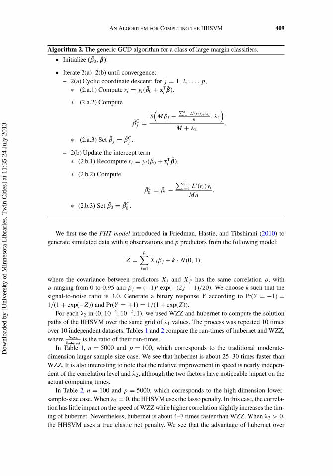
Algorithm 2. The generic GCD algorithm for a class of large margin classifiers.

• Initialize (β0, β).

• Iterate 2(a)–2(b) until convergence:– 2(a) Cyclic coordinate descent: for j = 1, 2, . . . , p,

∗ (2.a.1) Compute ri = yi(β0 + xᵀi β).

∗ (2.a.2) Compute

βCj =

S(Mβj −

∑ni=1 L′(ri )yixij

n, λ1

)M + λ2

.

∗ (2.a.3) Set βj = βCj .

– 2(b) Update the intercept term∗ (2.b.1) Recompute ri = yi(β0 + xᵀ

i β).

∗ (2.b.2) Compute

βC0 = β0 −

∑ni=1 L′(ri)yi

Mn.

∗ (2.b.3) Set β0 = βC0 .

We first use the FHT model introduced in Friedman, Hastie, and Tibshirani (2010) togenerate simulated data with n observations and p predictors from the following model:

Z =p∑

j=1

Xjβj + k · N (0, 1),

where the covariance between predictors Xj and Xj ′ has the same correlation ρ, withρ ranging from 0 to 0.95 and βj = (−1)j exp(−(2j − 1)/20). We choose k such that thesignal-to-noise ratio is 3.0. Generate a binary response Y according to Pr(Y = −1) =1/(1 + exp(−Z)) and Pr(Y = +1) = 1/(1 + exp(Z)).

For each λ2 in (0, 10−4, 10−2, 1), we used WZZ and hubernet to compute the solutionpaths of the HHSVM over the same grid of λ1 values. The process was repeated 10 timesover 10 independent datasets. Tables 1 and 2 compare the run-times of hubernet and WZZ,where tWZZ

thubernetis the ratio of their run-times.

In Table 1, n = 5000 and p = 100, which corresponds to the traditional moderate-dimension larger-sample-size case. We see that hubernet is about 25–30 times faster thanWZZ. It is also interesting to note that the relative improvement in speed is nearly indepen-dent of the correlation level and λ2, although the two factors have noticeable impact on theactual computing times.

In Table 2, n = 100 and p = 5000, which corresponds to the high-dimension lower-sample-size case. When λ2 = 0, the HHSVM uses the lasso penalty. In this case, the correla-tion has little impact on the speed of WZZ while higher correlation slightly increases the tim-ing of hubernet. Nevertheless, hubernet is about 4–7 times faster than WZZ. When λ2 > 0,the HHSVM uses a true elastic net penalty. We see that the advantage of hubernet over

Dow

nloa

ded

by [

Uni

vers

ity o

f M

inne

sota

Lib

rari

es, T

win

Citi

es]

at 1

1:35

24

July

201

3

410 Y. YANG AND H. ZOU

Table 1. Timings (in seconds) for WZZ and hubernet for n = 5000, p = 100 data. Total time over the same gridof λ1 values chosen by WZZ, averaged over 10 independent runs

n = 5000, p = 100

ρ 0 0.1 0.2 0.5 0.8 0.95

λ2 = 0WZZ 88.42 85.51 86.97 86.56 96.24 113.83hubernet 2.97 2.87 2.93 2.84 3.21 4.03

tWZZthubernet

29.79 29.68 30.48 29.98 28.25 28.25

λ2 = 10−4

WZZ 87.87 84.93 86.43 86.08 95.78 113.24hubernet 2.99 2.87 2.93 2.86 3.24 4.05

tWZZthubernet

29.39 29.59 29.50 30.10 29.56 27.96

λ2 = 10−2

WZZ 80.53 76.65 79.38 78.73 87.45 107.24hubernet 2.68 2.59 2.65 2.57 2.96 3.81

tWZZthubernet

30.05 29.59 29.95 30.63 29.54 28.15

λ2 = 1WZZ 12.43 12.37 12.37 12.37 12.54 27.54hubernet 0.45 0.48 0.49 0.50 0.53 1.03

tWZZthubernet

27.62 25.77 25.24 24.74 23.66 26.74

WZZ increases as λ2 becomes larger. A closer examination shows that WZZ is significantlylowered down by a larger λ2, while λ2 has a much weaker impact on hubernet’s timings.

We now use some popular benchmark datasets to compare WZZ and hubernet. Fivedatasets were considered in this study (see Table 3 for details). The first dataset Arcene

Table 2. Timings (in seconds) for WZZ and hubernet for n = 100, p = 5000 data. Total time over the same gridof λ1 values chosen by WZZ, averaged over 10 independent runs

n = 100, p = 5000

ρ 0 0.1 0.2 0.5 0.8 0.95

λ2 = 0WZZ 5.86 5.67 5.93 5.56 5.73 5.54hubernet 0.87 0.82 0.86 0.86 1.01 1.16

tWZZthubernet

6.74 6.91 6.90 6.47 5.67 4.78

λ2 = 10−4

WZZ 208.39 208.13 203.15 208.46 203.87 188.75hubernet 2.71 2.69 2.70 2.76 2.94 3.01

tWZZthubernet

76.90 77.37 75.24 75.53 69.34 62.71

λ2 = 10−2

WZZ 256.96 256.76 255.94 257.79 252.89 234.48hubernet 2.97 2.96 3.03 2.95 2.95 2.96

tWZZthubernet

86.52 86.74 84.47 87.39 85.73 79.22

λ2 = 1WZZ 292.75 292.87 292.91 292.84 291.45 282.51hubernet 2.63 2.64 2.61 2.56 2.46 2.41

tWZZthubernet

111.31 110.94 112.23 114.39 118.48 117.22

Dow

nloa

ded

by [

Uni

vers

ity o

f M

inne

sota

Lib

rari

es, T

win

Citi

es]

at 1

1:35

24

July

201

3

AN ALGORITHM FOR COMPUTING THE HHSVM 411

Table 3. Timings (in seconds) of WZZ and hubernet for some benchmark real data, averaged over 10 runs

HHSVM on benchmark datasets

Data n p WZZ hubernet tWZZthubernet

Arcene 100 10000 37.17 2.46 15.09Breast cancer 42 22283 3.16 0.46 6.85Colon 62 2000 14.17 0.42 33.96Leukemia 72 7128 52.20 1.42 36.69Prostate 102 6033 302.91 3.47 87.2

is obtained from UCI Machine Learning Repository (Frank and Asuncion 2010). We alsoconsidered the breast cancer data in Graham et al. (2010), the colon cancer data in Alon et al.(1999), the leukemia data in Golub et al. (1999), and the prostate cancer data in Singh et al.(2002). For each dataset, we randomly split the data into a training set and a test set withratio 4:1. The HHSVM was trained and tuned by five-fold cross-validation on the trainingset. Note that we did a two-dimensional cross-validation to find the best pair of (λ2, λ1) thatincurs minimal misclassification error. Let λCV

2 denote the chosen λ2 by cross-validation.We reported the timing of WZZ and hubernet for computing solution paths of the HHSVMwith λ2 = λCV

2 . The whole process was repeated 10 times. As can be seen from Table 3,hubernet is much faster than WZZ in all examples. It is also interesting to see that hubernetis very fast on all five datasets but WZZ can be very slow on prostate data.

5.2 COMPARING HUBERNET, SQSVMNET, AND LOGITNET

As shown in Section 4, the GCD algorithm provides a unified solution to three elasticnet penalized large margin classifiers using Huberized hinge loss, squared hinge loss, andlogistic regression loss. Here we compare the run times of hubernet for the HHSVM,sqsvmnet for the elastic net penalized squared hinge loss, and logitnet for the elastic netpenalized logistic regression. We want to see how the loss function affects the computingtime of GCD.

For the elastic net penalized logistic regression, Friedman, Hastie, and Tibshirani (2010)had developed a very efficient algorithm by combining Newton–Raphson and penalizedweighted least squares. Their software is available in the R package glmnet. However glmnet

uses a different form of the elastic net penalty: Pλ,α(β) = λ∑p

j=1

[12 (1 − α)β2

j + α|βj |].

Fortunately, the glmnet code can be easily modified for the elastic net penalty Pλ1,λ2 (β) in(2.4). We have reimplemented glmnet and denote it by logitnet-FHT for notation conve-nience.

We first use the FHT model to generate simulation data with n = 100, p = 5000. Table 4shows the run times (in seconds) of hubernet (δ = 2), hubernet (δ = 0.01), sqsvmnet,logitnet, and logitnet-FHT. Each method solves the solution paths for 100 λ1 values for each(λ2, ρ) combination. First of all, Table 4 shows that all these methods are computationallyefficient. Relatively speaking, the Huberized hinge loss (δ = 2) and squared hinge loss leadto the fastest classifiers computed by GCD. As argued in Section 2.4, hubernet (δ = 0.01)can be used to approximate the elastic net penalized SVM. Compared with the defaulthubernet (with δ = 2), hubernet (δ = 0.01) is about 10 times slower.

Dow

nloa

ded

by [

Uni

vers

ity o

f M

inne

sota

Lib

rari

es, T

win

Citi

es]

at 1

1:35

24

July

201

3

412 Y. YANG AND H. ZOU

Table 4. Timings (in seconds) for hubernet (δ = 2), hubernet (δ = 0.01), sqsvmnet, logitnet, and logitnet-FHTin the elastic net penalized classification methods for n = 100, p = 5000 data. Total time for 100 values of λ1,averaged over 10 independent runs

ρ 0 0.1 0.2 0.5 0.8 0.95

λ2 = 0hubernet (δ = 2) 0.64 0.63 0.65 0.65 0.81 0.89hubernet (δ = 0.01) 6.25 5.46 5.87 7.21 9.11 8.92sqsvmnet 0.49 0.47 0.48 0.50 0.59 0.65logitnet 3.85 3.85 3.82 4.77 6.06 8.02logitnet-FHT 0.48 0.50 0.54 0.62 0.81 1.24

λ2 = 10−4

hubernet (δ = 2) 0.64 0.62 0.64 0.67 0.81 0.88hubernet (δ = 0.01) 6.20 5.62 5.71 6.76 8.60 8.94sqsvmnet 0.50 0.50 0.50 0.53 0.62 0.68logitnet 3.78 3.81 3.79 4.69 6.07 8.05logitnet-FHT 0.48 0.50 0.54 0.62 0.81 1.23

λ2 = 10−2

hubernet (δ = 2) 0.83 0.72 0.80 0.78 0.79 0.87hubernet (δ = 0.01) 6.07 5.31 5.38 7.05 9.47 9.39sqsvmnet 0.51 0.47 0.47 0.50 0.58 0.63logitnet 4.24 4.18 4.49 5.11 7.29 8.14logitnet-FHT 0.51 0.52 0.56 0.63 0.80 1.15

λ2 = 1hubernet (δ = 2) 0.76 0.75 0.72 0.72 0.76 0.76hubernet (δ = 0.01) 12.92 13.29 13.69 15.69 20.99 11.45sqsvmnet 0.64 0.61 0.60 0.62 0.74 0.73logitnet 4.89 4.63 4.53 4.69 4.98 5.17logitnet-FHT 0.78 0.74 0.76 0.75 0.71 0.77

We also observe that logitnet-FHT is about 8–10 times faster than logitnet. A possibleexplanation is that logitnet-FHT takes advantages of the Hessian matrix of the logisticregression model in its Newton–Raphson step, while logitnet simply uses 1/4 to replacethe second derivatives, which can be conservative. On the other hand, hubernet (δ = 2) andsqsvmnet are at least comparable to logitnet-FHT and the former two even have noticeableadvantages when the correlation is high.

We now compare timings and classification accuracy of hubernet (δ = 2), hubernet(δ = 0.01), sqsvmnet, logitnet, and logitnet-FHT on the five benchmark datasets (See detailsin Table 5). Each model was trained and tuned in the same way as described in Section 5.1.Average misclassification error on the test set from 10 independent splits is reported. Alsoreported is the run time (in seconds) for computing the solution paths with λ2 chosen byfive-fold cross-validation. We can see that the hubernet with δ = 2 or δ = 0.01 has betterclassification accuracy than other classifiers on Arcene, Colon, Leukemia, and Prostate,while sqsvmnet has the smallest error on breast cancer. In terms of timings, there arethree datasets for which sqsvmnet is the winner and logitnet-FHT wins on the other two.The timing results for hubernet (δ = 2) are very close to those of sqsvmnet and logitnet-FHT. Overall, hubernet (δ = 2) delivers very competitive performance on these benchmarkdatasets.

Dow

nloa

ded

by [

Uni

vers

ity o

f M

inne

sota

Lib

rari

es, T

win

Citi

es]

at 1

1:35

24

July

201

3

AN ALGORITHM FOR COMPUTING THE HHSVM 413

Table 5. Testing error (%) and timings (in seconds) for some benchmark real data. The timings are for computingsolution paths for hubernet (δ = 2), hubernet (δ = 0.01), sqsvmnet, logitnet, and logitnet-FHT with λ2 chosen bycross-validation and over the grid of 100 λ1 values, averaged over 10 runs

Classification methods comparison on real data

Arcene Breast cancer Colon Leukemia Prostate

Method Error Time Error Time Error Time Error Time Error Time

hubernet (δ = 2) 21.00 1.35 19.71 1.12 17.90 0.23 3.16 0.73 9.35 0.77hubernet (δ = 0.01) 23.58 23.92 19.71 15.36 15.10 7.35 2.41 5.55 8.47 6.12sqsvmnet 23.00 1.13 19.14 1.15 19.30 0.18 3.25 0.54 8.88 0.66logitnet 25.00 9.71 19.57 6.53 21.20 1.13 3.91 6.23 9.05 4.77logitnet-FHT 25.00 1.85 19.57 1.08 21.20 0.14 3.91 0.65 9.05 0.67

6. DISCUSSION

In this article, we have presented a GCD algorithm for efficiently computing the solutionpaths of the HHSVM. We also generalized the GCD to other large margin classifiers anddemonstrated their performances. The GCD algorithm has been implemented in an Rpackage gcdnet, which is publicly available from The Comprehensive R Archive Networkat http://cran.r-project.org/web/packages/gcdnet/index.html.

As pointed out by a referee, in the optimization literature, there are other efficient al-gorithms for solving the HHSVM and the elastic net penalized squared SVM, logisticregression. Tseng (2009) proposed a coordinate gradient descent method for solving �1 pe-nalized smooth optimization problems. Nesterov (2007) proposed the composite gradientmapping idea for minimizing the sum of a smooth convex function and a nonsmooth con-vex function such as the �1 penalty. These algorithms can be applied to the large marginclassifiers considered in this article. We do not argue here that GCD is superior than thesealternatives. The message we wish to convey is that the marriage between coordinate de-scent and MM principle could yield an elegant, stable, and yet very efficient algorithm forhigh-dimensional classification.

SUPPLEMENTARY MATERIALS

The supplementary materials are available in a single zip file, which contains the R packagegcdnet and a readme file (README.txt).

ACKNOWLEDGMENTS

The authors thank the editor, an associate editor, and two referees for their helpful comments and suggestions.This work is supported in part by NSF grant DMS-08-46068.

[Received October 2011. Revised March 2012.]

REFERENCES

Alon, U., Barkai, N., Notterman, D., Gish, K., Ybarra, S., Mack, D., and Levine, A. (1999), “Broad Patterns of GeneExpression Revealed by Clustering Analysis of Tumor and Normal Colon Tissues Probed by OligonucleotideArrays,” Proceedings of the National Academy of Sciences, 96, 6745–6750. [411]

Dow

nloa

ded

by [

Uni

vers

ity o

f M

inne

sota

Lib

rari

es, T

win

Citi

es]

at 1

1:35

24

July

201

3

414 Y. YANG AND H. ZOU

Bradley, P., and Mangasarian, O. (1998), “Feature Selection via Concave Minimization and Support VectorMachines,” in Machine Learning Proceedings of the Fifteenth International Conference (ICML’98), pp.82–90.

Buhlmann, P., and van de Geer, S. (2011), Statistics for High Dimensional Data, Heidelberg: Springer. [396]

Burges, C. (1998), “A Tutorial on Support Vector Machines for Pattern Recognition,” Data Mining and Knowledge

Discovery, 2, 121–167. [399]

Daubechies, I., Defrise, M., and De Mol, C. (2004), “An Iterative Thresholding Algorithm for Linear InverseProblems With a Sparsity Constraint,” Communications on Pure and Applied Mathematics, 57, 1413–1457.[397]

De Leeuw, J., and Heiser, W. (1977), “Convergence of Correction Matrix Algorithms for MultidimensionalScaling,” in Geometric Representations of Relational Data, ed. J. C. Lingoes, Ann Arbor, MI: Mathesis Press,pp. 735–752.

Dempster, A., Laird, N., and Rubin, D. (1977), “Maximum Likelihood From Incomplete Data via the EMAlgorithm,” Journal of the Royal Statistical Society, Series B, 39, 1–38. [404]

Efron, B., Hastie, T., Johnstone, I., and Tibshirani, R. (2004), “Least Angle Regression,” The Annals of Statistics,32, 407–451. [397]

Evgeniou, T., Pontil, M., and Poggio, T. (2000), “Regularization Networks and Support Vector Machines,”Advances in Computational Mathematics, 13, 1–50. [399]

Frank, A., and Asuncion, A. (2010), “Arcene Data Set: UCI” Machine Learning Repository, Available athttp://archive.ics.uci.edu/ml/datasets/Arcene.

Friedman, J., Hastie, T., Hofling, H., and Tibshirani, R. (2007), “Pathwise Coordinate Optimization,” The Annalsof Applied Statistics, 1, 302–332. [397]

Friedman, J., Hastie, T., and Tibshirani, R. (2010), “Regularization Paths for Generalized Linear Models viaCoordinate Descent,” Journal of Statistical Software, 33, 1. [397,401,403,409,411]

Fu, W. (1998), “Penalized Regressions: The Bridge Versus the Lasso,” Journal of Computational and Graphical

Statistics, 7, 397–416. [397]

Genkin, A., Lewis, D., and Madigan, D. (2007), “Large-Scale Bayesian Logistic Regression for Text Categoriza-tion,” Technometrics, 49, 291–304. [397]

Golub, T., Slonim, D., Tamayo, P., Huard, C., Gaasenbeek, M., Mesirov, J., Coller, H., Loh, M., Downing, J.,Caligiuri, M., Bloomfield, C., and Lander, E. (1999), “Molecular Classification of Cancer: Class Discoveryand Class Prediction by Gene Expression Monitoring,” Science, 286, 531–537. [411]

Graham, K., de las Morenas, A., Tripathi, A., King, C., Kavanah, M., Mendez, J., Stone, M., Slama, J., Miller,M., Antoine, G., Willers, H., Sebastiani, P., and Rosenberg, C. (2010), “Gene Expression in HistologicallyNormal Epithelium From Breast Cancer Patients and From Cancer-Free Prophylactic Mastectomy PatientsShares a Similar Profile,” British Journal of Cancer, 102, 1284–1293. [411]

Hastie, T., Tibshirani, R., and Friedman, J. (2001), The Elements of Statistical Learning: Data Mining, Inference,

and Prediction, New York: Springer Verlag. [396,399]

Hunter, D., and Lange, K. (2004), “A Tutorial on MM Algorithms,” The American Statistician, 58, 30–37. [404]

Lange, K., Hunter, D., and Yang, I. (2000), “Optimization Transfer Using Surrogate Objective Functions,” Journal

of Computational and Graphical Statistics, 9, 1–20. [404]

Nesterov, Y. (2007), “Gradient Methods for Minimizing Composite Objective Function,” Technical Report, Centerfor Operations Research and Econometrics (CORE), Catholic University of Louvain (UCL).

Osborne, M., Presnell, B., and Turlach, B. (2000), “A New Approach to Variable Selection in Least SquaresProblems,” IMA Journal of Numerical Analysis, 20, 389–404. [397]

Rosset, S., and Zhu, J. (2007), “Piecewise Linear Regularized Solution Paths,” The Annals of Statistics, 35,1012–1030. [397]

Singh, D., Febbo, P., Ross, K., Jackson, D., Manola, J., Ladd, C., Tamayo, P., Renshaw, A., D’Amico, A., Richie,J., Lander, E. S., Loda, M., Kantoff, P. W., Golub, T. R., and Sellers, W. R. (2002), “Gene ExpressionCorrelates of Clinical Prostate Cancer Behavior,” Cancer Cell, 1, 203–209. [397,411]

Dow

nloa

ded

by [

Uni

vers

ity o

f M

inne

sota

Lib

rari

es, T

win

Citi

es]

at 1

1:35

24

July

201

3

AN ALGORITHM FOR COMPUTING THE HHSVM 415

Tibshirani, R. (1996), “Regression Shrinkage and Selection via the Lasso,” Journal of the Royal Statistical Society,Series B, 58, 267–288. [396]

Tseng, P. (2001), “Convergence of a Block Coordinate Descent Method for Nondifferentiable Minimization,”Journal of Optimization Theory and Applications, 109, 475–494. [401]

Tseng, P., and Yun, S. (2009), “A coordinate Gradient Descent Method for Nonsmooth Separable Minimization,”Mathematical Programming, 117, 387–423. [413]

Van der Kooij, A. (2007), “Prediction Accuracy and Stability of Regression With Optimal Scaling Transforma-tions,” Ph.D. thesis, Child & Family Studies and Data Theory (AGP-D), Department of Education and ChildStudies, Faculty of Social and Behavioural Sciences, Leiden University.

Vapnik, V. (1995), The Nature of Statistical Learning Theory, New York: Springer-Verlag. [396,399]

Wang, L., Zhu, J., and Zou, H. (2008), “Hybrid Huberized Support Vector Machines for Microarray Classificationand Gene Selection,” Bioinformatics, 24, 412–419. [396,397,399,400,401,408]

Wu, T. T., and Lange, K. (2008), “Coordinate Descent Algorithms for Lasso Penalized Regression,” The Annals

of Applied Statistics, 2, 224–244. [397]

——— and Lange, K. (2010), “The MM Alternative to EM,” Statistical Science, 25, 492–505. [404]

Zhu, J., Rosset, S., Hastie, T., and Tibshirani, R. (2004), “1-Norm Support Vector Machines,” The Annual

Conference on Neural Information Processing Systems, 16.

Zou, H., and Hastie, T. (2005), “Regularization and Variable Selection via the Elastic Net,” Journal of the RoyalStatistical Society, Series B, 67, 301–320. [397,399,402]

Dow

nloa

ded

by [

Uni

vers

ity o

f M

inne

sota

Lib

rari

es, T

win

Citi

es]

at 1

1:35

24

July

201

3