Statistics, Data Analysis, and Simulation SS 2017 · Statistics, Data Analysis, and Simulation SS...

Statistics, Data Analysis, and SimulationSS 2017

08.128.730 Statistik, Datenanalyse und Simulation

Dr. Michael O. Distler<[email protected]>

Mainz, 4. Mai 2017

Dr. Michael O. Distler <[email protected]> Statistics, Data Analysis, and Simulation SS 2017 1 / 25

http://wwwa1.kph.uni-mainz.de/~distler/

mailto:[email protected]



Was wir bisher gelernt haben

Spezielle diskrete VerteilungenBinomialPoisson

Spezielle WahrscheinlichkeitsdichtenUniform (Gleichverteilung)Gaussian (Normal)Chi-squared




Gammaverteilung

Ziel ist die Berechnung der Wahrscheinlichkeitsdichte f (t) fürdie Zeitdifferenz t zwischen zwei Ereignissen, wobei dieEreignisse zufällig mit einer mittleren Rate λ auftreten. AlsBeispiel kann der radioaktive Zerfall mit einer mittlerenZerfallsrate λ dienen.Die Wahrscheinlichkeitsdichte der Gammaverteilung istgegeben durch

f (x ; k) =xk−1e−x

Γ(k)mit Γ(z) =

∫ ∞0

tz−1e−tdt ; Γ(z+1) = z!

und gibt die Verteilung der Wartezeit t = x vom ersten bis zumk -ten Ereignis in einem Poisson-verteilten Prozess mitMittelwert µ = 1 an. Die Verallgemeinerung für andere Wertevon µ ist

f (x ; k , µ) =xk−1µke−µx

Γ(k)




Gamma distribution

0

0.1

0.2

0.3

0.4

0.5

0.6

0.7

0.8

0.9

1

0 1 2 3 4 5

1.0*exp(-1.0*x)




Charakteristische Funktion

Ist x eine reelle Zufallsvariable mit der Verteilungsfunktion F (x)und der Wahrscheinlichkeitsdichte f (x), so bezeichnet man alsihre charakteristische Funktion den Erwartungswert der Größeexp(ıtx):

ϕ(t) = E [exp(ıtx)]

also im Fall einer kontinuierlichen Variablen ein Fourier-Integralmit seinen bekannten Transformationseigenschaften:

ϕ(t) =

∫ ∞−∞

exp(ıtx) f (x)dx ⇔ f (x) =1

2π

∫ ∞−∞

exp(−ıtx)ϕ(t)dt

Insbesondere gilt für die zentralen Momente:

µn = E [xn] =

∫ ∞−∞

xn f (x)dx

ϕ(n)(t) =dnϕ(t)

dtn = ın∫ ∞−∞

xn exp(ıtx) f (x)dx

ϕ(n)(0) = ınµn




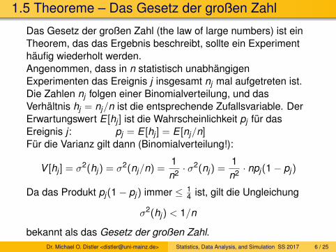
1.5 Theoreme – Das Gesetz der großen Zahl

Das Gesetz der großen Zahl (the law of large numbers) ist einTheorem, das das Ergebnis beschreibt, sollte ein Experimenthäufig wiederholt werden.Angenommen, dass in n statistisch unabhängigenExperimenten das Ereignis j insgesamt nj mal aufgetreten ist.Die Zahlen nj folgen einer Binomialverteilung, und dasVerhältnis hj = nj/n ist die entsprechende Zufallsvariable. DerErwartungswert E [hj ] ist die Wahrscheinlichkeit pj für dasEreignis j : pj = E [hj ] = E [nj/n]Für die Varianz gilt dann (Binomialverteilung!):

V [hj ] = σ2(hj) = σ2(nj/n) =1n2 · σ

2(nj) =1n2 · npj(1− pj)

Da das Produkt pj(1− pj) immer ≤ 14 ist, gilt die Ungleichung

σ2(hj) < 1/n

bekannt als das Gesetz der großen Zahl.Dr. Michael O. Distler <[email protected]> Statistics, Data Analysis, and Simulation SS 2017 6 / 25



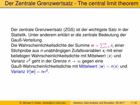
Der Zentrale Grenzwertsatz - The central limit theorem

Der zentrale Grenzwertsatz (ZGS) ist der wichtigste Satz in derStatistik. Unter anderem erklärt er die zentrale Bedeutung derGauß-Verteilung.Die Wahrscheinlichkeitsdichte der Summe w =

∑ni=1 xi einer

Stichprobe aus n unabhängigen Zufallsvariablen xi mit einerbeliebigen Wahrscheinlichkeitsdichte mit Mittelwert 〈x〉 undVarianz σ2 geht in der Grenze n→∞ gegen eineGauß-Wahrscheinlichkeitsdichte mit Mittelwert 〈w〉 = n〈x〉 undVarianz V [w ] = nσ2.




Illustration: Zentraler Grenzwertsatz

0

0.1

0.2

0.3

0.4

0.5

-3 -2 -1 0 1 2 3

GaussN=1

0

0.1

0.2

0.3

0.4

0.5

-3 -2 -1 0 1 2 3

N=2

0

0.1

0.2

0.3

0.4

0.5

-3 -2 -1 0 1 2 3

N=3

0

0.1

0.2

0.3

0.4

0.5

-3 -2 -1 0 1 2 3

N=10

Dargestellt ist die Summe uniform verteilter Zufallszahlen imVergleich zur Standardnormalverteilung.




1.6 Stichprobe - Sampling

eine zufällige (oder representative) Untermenge einer „Population“

li/cm ni ni li/cm ni l2i /cm2

18.9 1 18.9 357.2119.1 1 19.1 364.8119.2 2 38.4 737.2819.3 1 19.3 372.4919.4 4 77.6 1505.4419.5 3 58.5 1140.7519.6 9 176.4 3457.4419.7 8 157.6 3104.7219.8 11 217.8 4312.4419.9 9 179.1 3564.0920.0 5 100.0 2000.0020.1 7 140.7 2828.0720.2 8 161.6 3264.3220.3 9 182.7 3708.8120.4 6 122.4 2496.9620.5 3 61.5 1260.7520.6 2 41.2 848.7220.7 2 41.4 856.9820.8 2 41.6 865.2820.9 2 41.8 873.6221.0 4 84.0 1764.0021.2 1 21.2 449.44∑

100 2002.8 40133.62

Stichprobe bestehend aus 100 Messungen:

N =∑

ni = 100

Mittelwert? Varianz?

〈l〉 =1N

∑ni li = 20.028 cm

s2 =1

N − 1

(∑ni l2i −

1N

(∑ni li)2)

= 0.2176 cm2

l = 〈l〉 ± s√N

= (20.028± 0.047) cm

s = s ± s√2(N − 1)

= (0.466± 0.033) cm




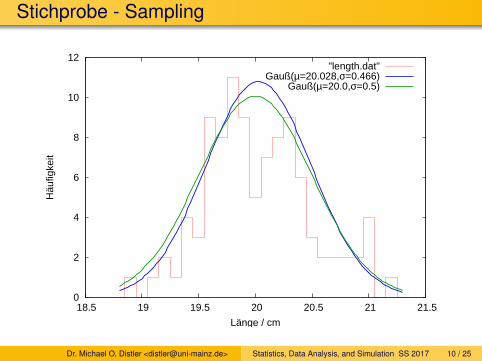
Stichprobe - Sampling

0

2

4

6

8

10

12

18.5 19 19.5 20 20.5 21 21.5

Häu

figke

it

Länge / cm

"length.dat"Gauß(µ=20.028,σ=0.466)

Gauß(µ=20.0,σ=0.5)




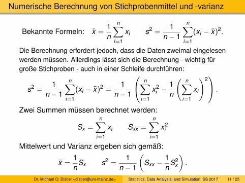
Numerische Berechnung von Stichprobenmittel und -varianz

Bekannte Formeln: x =1n

n∑i=1

xi s2 =1

n − 1

n∑i=1

(xi − x)2.

Die Berechnung erfordert jedoch, dass die Daten zweimal eingelesenwerden müssen. Allerdings lässt sich die Berechnung - wichtig fürgroße Stichproben - auch in einer Schleife durchführen:

s2 =1

n − 1

n∑i=1

(xi − x)2 =1

n − 1

n∑i=1

x2i −

1n

(n∑

i=1

xi

)2 .

Zwei Summen müssen berechnet werden:

Sx =n∑

i=1

xi Sxx =n∑

i=1

x2i

Mittelwert und Varianz ergeben sich gemäß:

x =1n

Sx s2 =1

n − 1

(Sxx −

1n

S2x

).




Numerische Berechnung von Stichprobenmittel und -varianz

Unter Umständen müssen dabei große Zahlen voneinanderabgezogen werden. Je nach Darstellung von Zahlen auf demComputer kann dies zu numerischen Problemen führen. Daherist es besser eine grobe Schätzung des Mittelwertes xe (etwader erste Messwert) zu verwenden:

Tx =n∑

i=1

(xi − xe) Txx =n∑

i=1

(xi − xe)2

Damit erhält man:

x = xe +1n

Tx s2 =1

n − 1

(Txx −

1n

T 2x

).




1.7 Mehrdimensionale Verteilungen

1.7.1 Zufallsvariable in zwei DimensionenDie mehrdimensionale Wahrscheinlichkeitsdichte f (x , y) derzwei Zufallszahlen x und y ist definiert durch dieWahrscheinlichkeit, das Variablenpaar (x , y) in den Intervallena ≤ x < b und c ≤ y < d zu finden

P(a ≤ x < b, c ≤ y < d) =

∫ d

c

∫ b

af (x , y) dx dy

Normierung: ∫ ∞−∞

∫ ∞−∞

f (x , y) dx dy = 1

Gilt:f (x , y) = h(x) · g(y)

dann sind die zwei Zufallsvariablen unabhängig.




Zufallsvariable in zwei Dimensionen

Mittelwerte und Varianzen sind naheliegend (siehe 1. Dim):

< x >= E [x ] =

∫ ∫x f (x , y) dx dy =

∫x fy (x) dx

< y >= E [y ] =

∫ ∫y f (x , y) dx dy =

∫y fx (y) dy

V [x ] =

∫ ∫(x− < x >)2 f (x , y) dx dy = σ2

x

V [y ] =

∫ ∫(y− < y >)2 f (x , y) dx dy = σ2

y

Sei z eine Funktion von x , y :

z = z(x , y)

Damit ist z ebenfalls eine Zufallsvariable.

< z > =

∫ ∫z(x , y) f (x , y) dx dy

σ2z =

⟨(z− < z >)2

⟩Dr. Michael O. Distler <[email protected]> Statistics, Data Analysis, and Simulation SS 2017 14 / 25




Einfaches Beispiel:

z(x , y) = a · x + b · y

< z > = a∫ ∫

x f (x , y) dx dy + b∫ ∫

y f (x , y) dx dy

= a < x > + b < y >

unproblematisch





z(x , y) = a · x + b · yVarianz:

σ2z =

⟨((a · x + b · y)− (a < x > + b < y >))2

⟩=

⟨((a · x − a < x >) + (b · y − b < y >))2

⟩= a2

⟨(x− < x >)2

⟩︸︷︷︸

σ2x

+b2⟨

(y− < y >)2⟩

︸︷︷︸σ2

y

+2ab 〈(x− < x >)(y− < y >)〉︸︷︷︸??

< (x− < x >)(y− < y >) >= cov(x , y) Kovarianz

= σxy =

∫ ∫(x− < x >)(y− < y >) f (x , y) dx dy





„Normalisierte“ Kovarianz:cov(x , y)

σx σy= ρxy Korrelationskoeffizient

ist ein dimensionsloses Maß für den Grad der Korrelationzweier Variablen: −1 ≤ ρxy ≤ 1





Für die Determinante der Kovarianzmatrix gilt:∣∣∣∣ σ2x σxy

σxy σ2y

∣∣∣∣ = σ2xσ

2y − σ2

xy = σ2xσ

2y (1− ρ2) ≥ 0




2-dim Gauß-Verteilung

-3.3

-3.2

-3.1

-3

-2.9

-2.8

-2.7

1.85 1.9 1.95 2 2.05 2.1 2.15

Para

met

er a

2

Parameter a1

Der Wahrscheinlichkeitsinhalt der Kovarianz-Ellipse: 39.3%




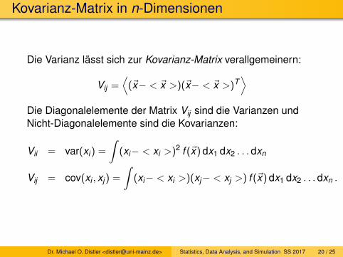
Kovarianz-Matrix in n-Dimensionen

Die Varianz lässt sich zur Kovarianz-Matrix verallgemeinern:

Vij =⟨

(~x− < ~x >)(~x− < ~x >)T⟩

Die Diagonalelemente der Matrix Vij sind die Varianzen undNicht-Diagonalelemente sind die Kovarianzen:

Vii = var(xi) =

∫(xi− < xi >)2 f (~x) dx1 dx2 . . . dxn

Vij = cov(xi , xj) =

∫(xi− < xi >)(xj− < xj >) f (~x) dx1 dx2 . . . dxn .




Kovarianz-Matrix in n-Dimensionen

Die Kovarianz-Matrix

Vij =

var(x1) cov(x1, x2) . . . cov(x1, xn)

cov(x2, x1) var(x2) . . . cov(x2, xn). . . . . . . . .

cov(xn, x1) cov(xn, x2) . . . var(xn)

ist eine symmetrische n × n Matrix:

Vij =

σ2

1 σ12 . . . σ1nσ21 σ2

2 . . . σ2n. . . . . . . . .

σn1 σn2 . . . σ2n




1.8 Transformation von Wahrscheinlichkeitsdichten

Die Funktion einer Zufallsvariablen ist selbst wieder eineZufallsvariable. Die Wahrscheinlichkeitsdichte fx (x) derVariablen x soll vermöge y = y(x) in eine andere Variable ytransformiert werden:

fx (x)y = y(x)

−→fy (y)

Betrachte: Intervall (x , x + dx)→ (y , y + dx)Bedenke: Die Flächen unter den Wahrscheinlichkeitsdichten inden jeweiligen Intervallen müssen gleich sein.

fx (x)dx = fy (y)dy ↪→ fy (y) = fx (x(y))

∣∣∣∣dxdy

∣∣∣∣




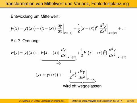
Transformation von Mittelwert und Varianz, Fehlerfortplanzung

Entwicklung um Mittelwert:

y(x) = y(〈x〉) + (x −〈x〉) dydx

∣∣∣∣x=〈x〉

+12

(x −〈x〉)2 d2ydx2

∣∣∣∣x=〈x〉

+ . . .

Bis 2. Ordnung:

E [y ] ' y(〈x〉) + E [x − 〈x〉] dydx

∣∣∣∣x=〈x〉︸︷︷︸

=0

+12

E [(x − 〈x〉)2]d2ydx2

∣∣∣∣x=〈x〉

〈y〉 ' y(〈x〉) +12σ2

xd2ydx2

∣∣∣∣x=〈x〉︸︷︷︸

wird oft weggelassen




Fehlerfortplanzung

Für die Varianz nehmen wir an 〈y〉 ' y(〈x〉) und entwickelny(x) um den Mittelwert 〈x〉 bis zur 1. Ordnung:

V [y ] = E[(y − 〈y〉)2

]= E

((x − 〈x〉) dydx

∣∣∣∣x=〈x〉

)2

=

(dydx

∣∣∣∣x=〈x〉

)2

· E[(x − 〈x〉)2

]=

(dydx

∣∣∣∣x=〈x〉

)2

· σ2x

Gesetz der Fehlerfortpflanzung für eine Zufallsvariable.




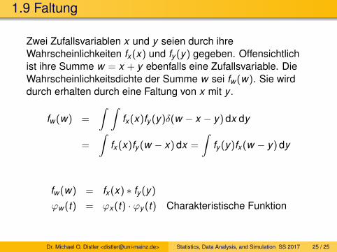
1.9 Faltung

Zwei Zufallsvariablen x und y seien durch ihreWahrscheinlichkeiten fx (x) und fy (y) gegeben. Offensichtlichist ihre Summe w = x + y ebenfalls eine Zufallsvariable. DieWahrscheinlichkeitsdichte der Summe w sei fw (w). Sie wirddurch erhalten durch eine Faltung von x mit y .

fw (w) =

∫ ∫fx (x)fy (y)δ(w − x − y) dx dy

=

∫fx (x)fy (w − x) dx =

∫fy (y)fx (w − y) dy

fw (w) = fx (x) ∗ fy (y)

ϕw (t) = ϕx (t) · ϕy (t) Charakteristische Funktion




Statistics, Data Analysis, and Simulation SS 2017 · Statistics, Data Analysis, and Simulation SS...

Documents

Transcript of Statistics, Data Analysis, and Simulation SS 2017 · Statistics, Data Analysis, and Simulation SS...