Statistics and Quantitative Analysis U4320 Segment 6 Prof. Sharyn O’Halloran.

Statistics and Quantitative Analysis U4320

Segment 6 Prof. Sharyn O’Halloran

I. Introduction A. Review of Population and Sample Estimates

Population Sample

Mean X

N

ii

N

1 X

X

n

ii

n

1

Variance

2

2

1

( )X

N

ii

N

s

X X

n

ii

n

2

2

1

1

( )

B. Sampling 1. Samples

The sample mean is a random variable with a normal distribution.

If you select many samples of a certain size then on average you will probably get close to the true population mean.

I. Introduction (cont.)

2. Central Limit Theorem

Definition

If a Random Sample is taken from any population with mean_ and standard deviation_, then the sampling distribution of the sample means will be normally distributed with

1) Sample Mean E() = _, and 2) Standard Error SE() = _/_n

As n increases, the sampling distribution of tends toward the true population mean_.

I. Introduction (cont.)

C. Making Inferences

To make inferences about the population from a given sample, we have to make one correction, instead of dividing by the standard deviation, we divided by the standard error of the sampling process:

Today, we want to develop a tool to determine how confident we are that our estimates lie within a certain range.

ZXSE

.

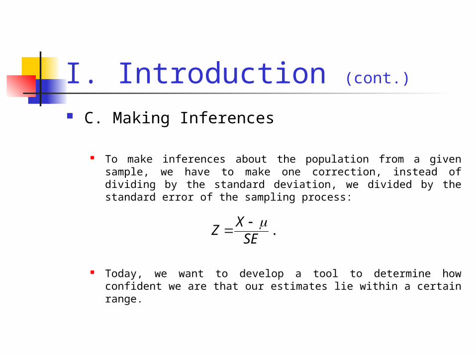
II. Confidence Interval A. Definition of 95% Confidence Interval

(_ known) 1. Motivation

We know that, on average, is equal to_. We want some way to express how confident we are that a

given is near the actual_ of the population. We do this by constructing a confidence interval, which is

some range around that most probably contains_. The standard error is a measure of how much error there is

in the sampling process. So we can say that is equal to__ the standard error

= X_Standard Error

II. Confidence Interval (cont.)

2. Constructing a 95% Confidence Interval

a. Graph

First, we know that the sample mean is distributed normally, with mean_ and standard error

SE=n

.

SE


b. Second, we determine how confident we want to be in our estimate of_

Defining how confident you want to be is called the -level.

So a 95% confidence interval has an associate - level of .05.

Because we are concerned with both higher and lower values, the relevant range is _/2 probability in each tail.

= (1-.95) = .05 5% level

SE


C. Define a 95% Confidence Range Now let's take an interval around that contains 95% of

the area under the curve. So if we take a random sample of size n from the

population, 95% of the time the population mean _ will be within the range:

[-z.025 * SE , z.025 * SE]

What is a z value associated with a .025 probability? From the z-table, we find the z-value associated with

a .025 probability is 1.96. So our range will be bounded by:

[-1.96 * SE , 1.96 * SE].


Now, let's take this interval of size [-1.96 * SE , 1.96 * SE] and use it as a measuring rod.

d. Interpreting Confidence Intervals

SE

-1.96*SE 1.96*SE

SE

-1.96*SE 1.96*SEX1X2X3


What's the probability that the population mean will fall within the interval 1.96 * SE?

e. In General

We get the actual interval as 1.96 * SE on either side of the sample mean .

We then know that 95% of the time, this interval will contain . This interval is defined by:

X - (Z.025 * /n) < < X + (Z.025 * /n)

= X Z /2 * SE


For a 95% confidence interval:

Examples

1. Example 1: Calculate a 95% confidence Interval

Say we sample n=180 people and see how many times they ate at a fast-food restaurant in a given week. The sample had a mean of 0.82 and the population standard deviation is 0.48. Calculate the 95% confidence interval for these data.

= X Z.025 * SE

= X 1.96 * SE


Answer:

Why 95%?

SE = .48 / 180 = 0.036.

z.025 * SE = 1.96 * .036 = .07

C.I. = .82 .07 OR [.75 < < .89]

SE = .036

-1.96*.036= .75 1.96*.036=.89.82


2. Example 2: Calculating a 90% confidence interval

A random sample of 16 observations was drawn from a normal population with = 6 and = 25. Find a 90% ( = .10) confidence interval for the population mean, _.

First, find Z.10/2 in the standard normal tables

Z.05 = 1.64


Second, calculate the 90% confidence interval

90% of the time, the mean will lie with in this range.

= X Z.05 * /n

= 25 1.64 * 6/16

SE= 1.5

= 25 1.64 * 1.5 = 25 2.46

22.53 < < 27.46


What if we wanted to be 99% of the time sure that the mean

falls with in the interval?

What happens when we move from a 90% to a 99% confidence

interval?

Z.005.= 2.58

25 2.58 * 1.5

25 3.87

21.13 < < 28.87

21.13 28.8722.53 27.46


C. Confidence Intervals (_ unknown)

1.Characteristics of a Student-t distribution

a.Shape the student t-distribution

The t-distribution changes shape as the sample size gets larger, and in the limit it becomes identical to the normal.

Normal Distribution

Student-t

.025Z .025Zt.025 t.025


b. When to use t-distribution i. is unknown ii. Sample size n is small

2. Constructing Confidence Intervals Using t-Distribution

A. Confidence Interval

95% confidence interval is:

B. Using t-tables

Say our sample size is n and we want to know what's the cutoff value to get 95% of the area under the curve.

X tsn

. .025

II. Confidence Interval (cont.) i) Find Degrees of Freedom

Degree of freedom is the amount of information used to calculate the standard deviation, s. We denote it as d.f. _ d.f. = n-1

ii) Look up in the t-table

Now we go down the side of the table to the degrees of freedom and across to the appropriate t-value.

That's the cutoff value that gives you area of .025 in each tail, leaving 95% under the middle of the curve.

iii) Example:

Suppose we have sample size n=15 and t.025 What is the critical value? 2.13


Answer: X = (64 + 66 + 89 + 77) / 4 = 74

s2 = (64-74)2 + (66-74)2 + (89-74)2 + (77-74)2 / 3 = 132.7

SE = sn

132 74

5 76.

.

d.f. = 3

t.025 = 3.18

t.025 * SE = 3.18 * 5.76 = 18

= X 1856 < < 92 (not very precise with a sample of only size 4)

7456 92


III. Differences of Means

A. Population Variance Known

Now we are interested in estimating the value (1 - 2) by the sample means, using 1 - 2.

Say we take samples of the size n1 and n2 from the two populations. And we want to estimate the differences in two population means.

To tell how accurate these estimates are, we can construct the familiar confidence interval around their difference:

( 1 - 2) = (X 1 - X 2) z.025 1

2

1

22

2n n .

II. Confidence Interval This would be the formula if the sample size were large

and we knew both 1 and 2.

B. Population Variance Unknown 1. If, as usual, we do not know 1 and 2, then we use the

sample standard deviations instead. When the variances of populations are not equal (s1 s2):

Example: Test scores of two classes where one is from an inner city school and the other is from

an affluent suburb.

(1 - 2) = (X 1 - X 2) t.025 sn

sn

12

1

22

2

.


2. Pooled Sample Variances, s1 = s2 ( is unknown)

If both samples come from the same population (e.g., test scores for two classes in the same school), we can assume that they have the same population variance . Then the formula becomes:

or just

In this case, we say that the sample variances are pooled. The formula for is:

( 1 - 2) = (X 1 - X 2) t.025 s

n

s

np p2

1

2

2

,

( 1 - 2) = (X 1 - X 2) t.025 s n np

1 1

1 2

.

sX X X X

n np2 1 1

22 2

2

1 21 1

( ) ( )

( ) ( )

sp2


The degrees of freedom are (n1-1) + (n2-1), or (n1+n2-2).

3. Example:

Two classes from the same school take a test. Calculate the 95% confidence interval for the difference between the two class means.

X1 X2

64 5666 7189 5377

X1/n= 296/4 = 74 X2/n= 180/3= 60


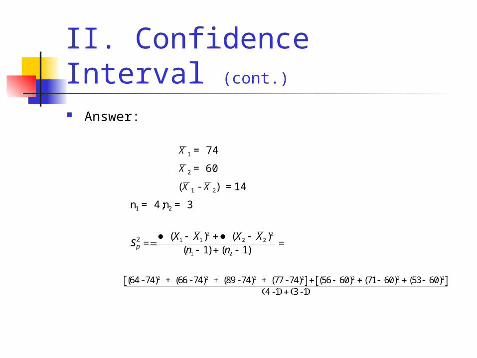
Answer:

X 1 = 74

X 2 = 60

(X 1 - X 2) = 14

n1 = 4; n2 = 3

sp2 =

( ) ( )( ) ( )

X X X Xn n

1 12

2 22

1 21 1 =

(64 - 74) + (66 - 74) + (89 - 74) + (77 - 74)4 -1 3 -1

2 2 2 2 2

( ) ( ) ( )56 60 71 60 53 602 2


sp2 = (398 + 186) / (3 + 2) = 117.

sp = 10.8

SE = s + p1 2

1

n

1

n 10 8

14

13

8 26. .

d.f. = 5

t.025 = 2.57

t.025 * SE = 2.57 * 8.26 = 21

(1 - 2) = (X 1 - X 2) 21 = 14 21

= -7 (1 - 2 35.

-7 351 2-


C. Matched Samples

1. Definition

Matched samples are ones where you take a single individual and measure him or her at two different points and then calculate the difference.

2. Advantage

One advantage of matched samples is that it reduces the variance because it allows the experimenter to control for many other variables which may influence the outcome.


3. Calculating a Confidence Interval

Now for each individual we can calculate their difference D from one time to the next.

We then use these D's as the data set to estimate , the population difference.

The sample mean of the differences will be denoted .

The standard error will just be:

Use the t-distribution to construct 95% confidence interval:SE = sD / n.

= D t.025 * sD/n.


4. Example:

Student X1 (Fall) X2 (Spring) D = X1-X2

Trimble 64 57 7Wilde 66 57 9Giannos 89 73 16Ames 77 65 12

D = (7 + 9 + 16 + 12) / 4 = 11

d.f. = n-1 = 3

s2D = (7-11)2 + (9-11)2 + (16-11)2 + (12-11)2 /3= 46/3

sD = 3.91

SE = sD / 4 = 3.91 / 2 = 1.96

t.025 = 3.18

t.025 * SE = 3.18 * 1.96 = 6


Notice that the standard error here is much smaller than in most of our unmatched pair examples.

So = D t.025 * sD/n.

= 11 6 = 5 to 17.

5 17

IV. Confidence Intervals for Proportions

Just before the 1996 presidential election, a Gallup poll of about 1500 voters showed 840 for Clinton and 660 for Dole. Calculate the 95% confidence interval for the population proportion of Clinton supporters.

Answer: n= 1500

Sample proportion P:

P = 840

150056.

IV. Confidence Intervals for Proportions (cont.)

Create a 95% confidence interval:

where and P are the population and sample proportions, and n is the

sample size.

That is, with 95% confidence, the proportion for Clinton in the whole

population of voters was between 53% and 59%.

= P sampling allowance

= P 1.96 P P

n

( )1,

= .56 1.96 . ( . )56 1 56

1500

,

= .56 .03.

Statistics and Quantitative Analysis U4320 Segment 6 Prof. Sharyn O’Halloran.

Documents

Transcript of Statistics and Quantitative Analysis U4320 Segment 6 Prof. Sharyn O’Halloran.