Statistics and Inference -...

Statistics and Inference in Astrophysics

Zhu & Menard (2013)

Today: brief intro to machine learning tools

Machine learning• Techniques to learn patterns in the data in flexible way; not parameter

inference

• Main tasks:

• Density estimation and clustering: What is the distribution of the data?

• Dimensionality reduction: What are the most important dimensions in the data?

• Regression: Learn to predict y(x) from (x,y) training data

• Classification: Learn to predict classification labels L from (x,L) training data

• Distinction between supervised and unsupervised learning

Density estimation• Have data points {xi} —> what is the density ρ(x)?

• Saw this in bootstrap: ρ(x) = 𝛴i δ(x-xi)

• Parametric: fit ρ(x) with some functional form with parameters θ, e.g., ρ(x) = N(x|mean,variance) —> use parameter-inference techniques from L2

• Non-parametric: Similar to sum-of-delta functions, but replace delta function with a different function —> build ρ(x) directly from the data without parameters

Simple parametric density estimation

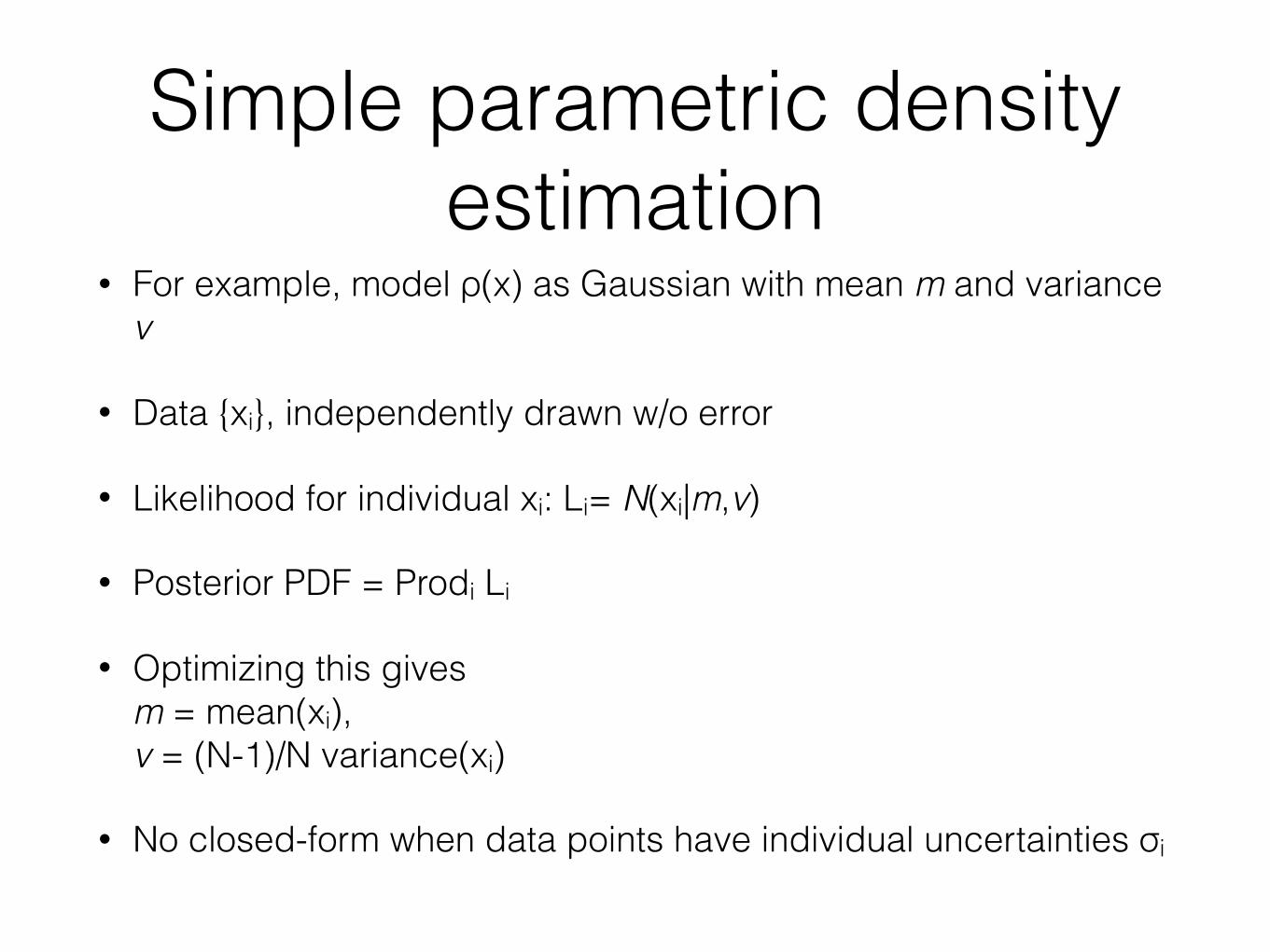
• For example, model ρ(x) as Gaussian with mean m and variance v

• Data {xi}, independently drawn w/o error

• Likelihood for individual xi: Li= N(xi|m,v)

• Posterior PDF = Prodi Li

• Optimizing this gives m = mean(xi), v = (N-1)/N variance(xi)

• No closed-form when data points have individual uncertainties σi

Simple non-parametric density estimation: histogram• A histogram is a form of density estimation

• Non-parametric because histogram per se does not have explicit parameters

• But have hyperparameters: location and width of bins that need to be chosen; hyperparameters don’t directly set the density, but constrain, e.g., it smoothness

• Widely used, but often doesn’t give a good representation of the data, non-smooth, and difficult in higher dimensions

Histogram example

Ivezic et al. (2014)

Same data, different binning!

Kernel density estimation (KDE)

• Remember from bootstrap: ρ(x) = 𝛴i δ(x-xi)

• Replace δ(.) with a kernel K(.) with width h x-xi with distance function d(x,xi):ρ(x) = 𝛴i K(d[x,xi]/hi)

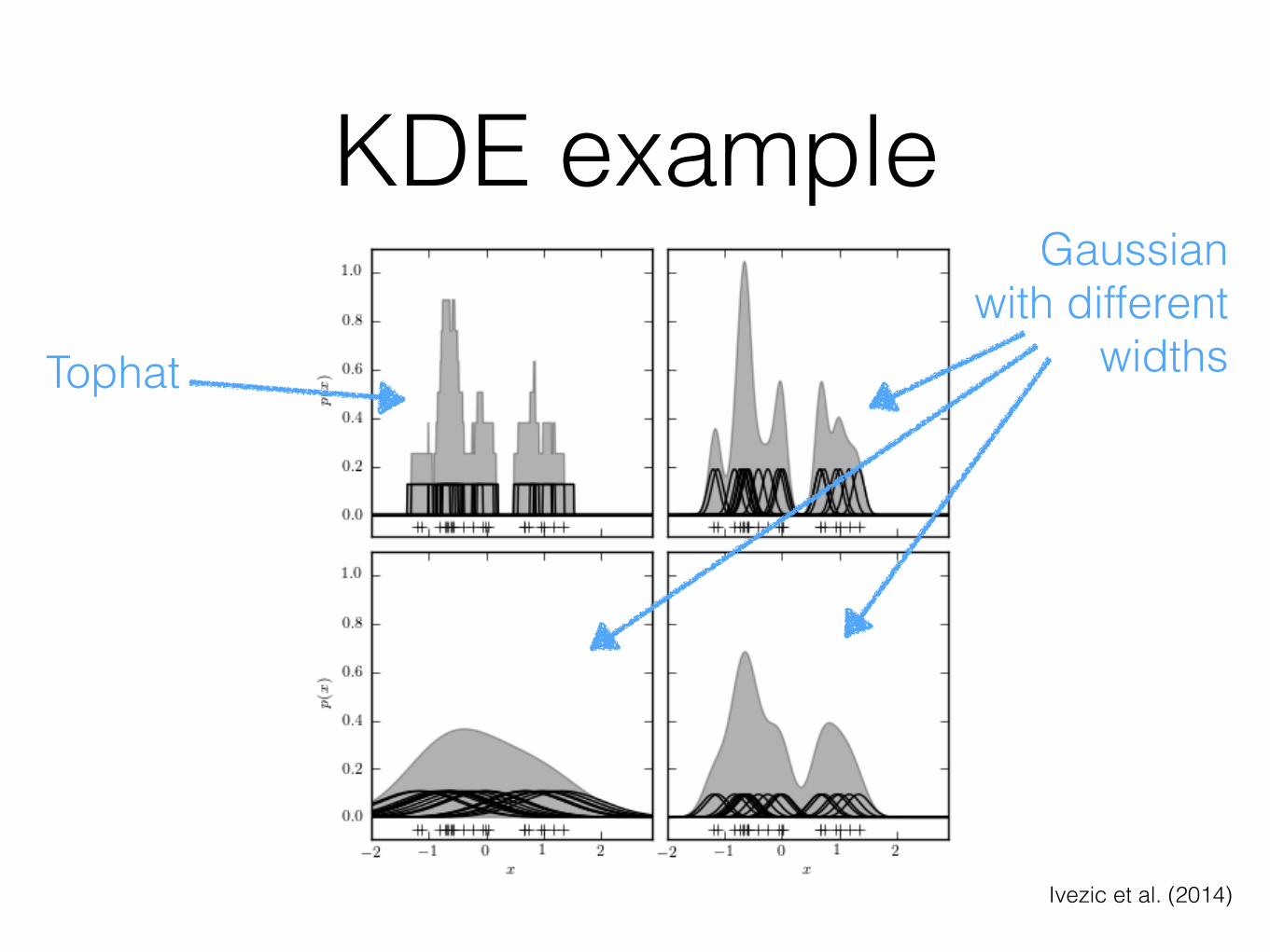
• K(.) could be: tophat function, similar to histogram, a Gaussian, or …

KDE example


Tophat

Gaussianwith different

widths

KDE: kernels• Kernels: symmetric functions around zero, positive

everywhere, integrate to 1

• Gaussian convenient, but has infinite support: need to always use all points to get a density evaluation

• Epanechnikov optimal in that it gives the smallest expected mean-squared-error:K(r = d(x,xi)) = 3(1-r2)/4, r <= 1 Brian Amberg/Wikipedia

KDE: bandwidth• Need to set width h of the kernel, this is a hyperparameter

• Some rules-of-thumb based on Gaussian data: Scott’s rule: h = N-1/(dim+4) [if data scaled to have unit variance] Silverman’s rule: h = [N*(dim+2)/4]-1/(dim+4) [same scaling]

• Other way: leave-one-out-cross-validation (see last lecture)

• Or minimize Mean-Integrated-Square-Error

• Can also have variable h that depends on the local density: h(x) = k / [ρ(x)]1/dim, higher density —> smaller kernel width

KDE applications• Easy-to-use and standard tool when you need to estimate

a density

• Examples:

• PDF from MCMC samples

• You have run a bunch of simulations that give points in some space (e.g., stellar tracks with MESA) and want to estimate a density covering the whole space

• But difficult to apply when data points have errors and want to deconvolve

Some examples…

Bovy et al. (2012)

MCMC chain —> KDE PDF Theoretical model points —> KDE density

Bovy et al. (2014)

Parametric density estimation with many parameters: Gaussian mixtures• Single Gaussian: strongly constrained parametric model;

KDE w/ Gaussian kernel: very flexible, but as many components as data points

• Gaussian Mixture Model (GMM): in between: model density ρ(x) as sum of K Gaussians, K < N

• Parameters: amplitudes, means, and variances of all Gaussians

• ρ(x) = 𝛴k ak N(x|mk,Vk)

• Could optimize likelihood for all parameters….

GMM and EM• When K becomes large, many parameters —> high-dimensional

parameter space to search for optimal solution

• Expectation-Maximization algorithm: General algorithm to optimize these kinds of problems

• Add a qik assignment variable to each data point: data point i drawn from component k where qik = 1 (all other qik= 0)

• If we knew all qi, then optimizing would be easy:ak = 1/N 𝛴i qikmeank = mean of those xi with qik = 1variancek = variance of those xi with qik = 1

• Expectation-maximization: Can show that following two steps always increase likelihood E(xpectation): qik = akN(xi|meank,variancek)/ [𝛴l alN(xi|meanl,variancel)]M(aximization): ak = 1/N 𝛴i qikmeank = 𝛴i qik xi / 𝛴i qikvariancek = 𝛴i qik (xi-meank)2 / 𝛴i qik

• Always leads to at least a local maximum, convergence very fast in general

GMM and EM

Gaussian mixture model• Parametric, but when K is large almost as flexible

as a non-parametric model

• Need to set K, the single hyper-parameter

• Use cross-validation or AIC/BIC

• If you are simply trying to get a good representation of a density, number K doesn’t matter as long as it’s big enough

Example


• Be careful when interpreting components!!

Gaussian mixtures with errors: extreme deconvolution (XD)

• If data have individual uncertainties (heteroskedastic uncertainties), can still fit a Gaussian mixture model quickly

• Trick is to include more hidden variables like the qik: true values xik if point i was drawn from component k

• Adds a few simple update steps (Bovy et al. 2011)

• Implemented in astroML, fast C version at github/jobovy/extreme-deconvolution

XD example


Clustering

• Example of unsupervised learning: given set of data xi, what are the clusters / classes that this data can be divided into?

• Could use a density estimate and find peaks or clearly separated points

• Simplest stand-by algorithm: K-means

K means• Fix number of clusters K

• Optimize 𝛴k 𝛴i in k |xi-mk|2

• Like Gaussian mixture model, but with hard assignments

• Optimization algorithm: 1. Start with set of {mk} 2. Assign each xi to its nearest mk3. Compute new mk as the mean of all of the xi assigned to cluster k 4. Go back to 2.

• Could also use medians: K medians

K means example


Clustering with Gaussian mixtures

• Can work much better because background can be fit out

Bovy et al. (2009)

Procedural clustering• Gaussian mixture and K-means have the advantage that they

optimize an objective function (the likelihood), so the outcome should not depend on how you found the optimal solution

• Procedural clustering defines clusters in a procedural way

• Hierarchical clustering: 1. Start with N clusters, N=#data 2. Join two clusters to form N-1 clusters3. Repeat

• Join based on: minimum distance between clusters (minimum spanning tree) —> extended clusters, maximum distance between clusters —> compact clusters, friends-of-friends is further example

Dimensionality reduction: PCA and ICA

Dimensionality reduction• Astronomical observations are by their nature high-

dimensional

• Need to focus on most important dimensions in the data

• Those dimensions are not necessarily aligned with observed axes, e.g., pixels in a spectrum


Principal Component Analysis (PCA)


• Data in D-dimensional space

• Find direction with highest variance

• Rotate such that that direction is x1

• In the remaining (D-1)-dimensional space do the same: find direction with highest variance, rotate that to x2

• and so on

Principal Component Analysis (PCA)

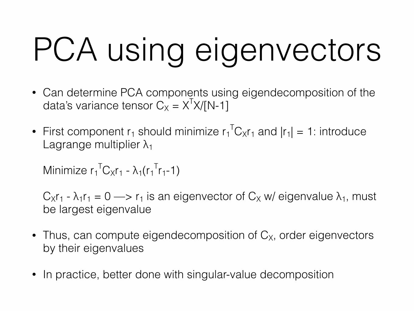
PCA using eigenvectors• Can determine PCA components using eigendecomposition of the

data’s variance tensor CX = XTX/[N-1]

• First component r1 should minimize r1TCXr1 and |r1| = 1: introduce

Lagrange multiplier λ1 Minimize r1

TCXr1 - λ1(r1Tr1-1)

CXr1 - λ1r1 = 0 —> r1 is an eigenvector of CX w/ eigenvalue λ1, must be largest eigenvalue

• Thus, can compute eigendecomposition of CX, order eigenvectors by their eigenvalues

• In practice, better done with singular-value decomposition

PCA example: galaxy spectra in SDSS


PCA in practice• Because you are rotating, technically only applies

when all dimensions have the same units

• If you want to apply PCA to dimensions with different units, need to divide out the units: subtract the mean and divide by typical value or ‘whiten’ by subtracting the mean and dividing by the data’s standard deviation

• If data have errors, need to account for this; if they are different for different dimensions and/or data points, need to solve for PCA components iteratively

Dimensionality reduction with PCA

• PCA decomposition tells you which directions explain most of the variation in the data

• Can cut at a certain number K <= D of PCA components that explain X% of the variance (K=D explains 100%)

• If K << D, can significantly reduce the dimensionality of the data

• Where to cut? Compare to expected noise level, or decide how much variance you want to explain, search for features in the (explained-variance) vs. K plot

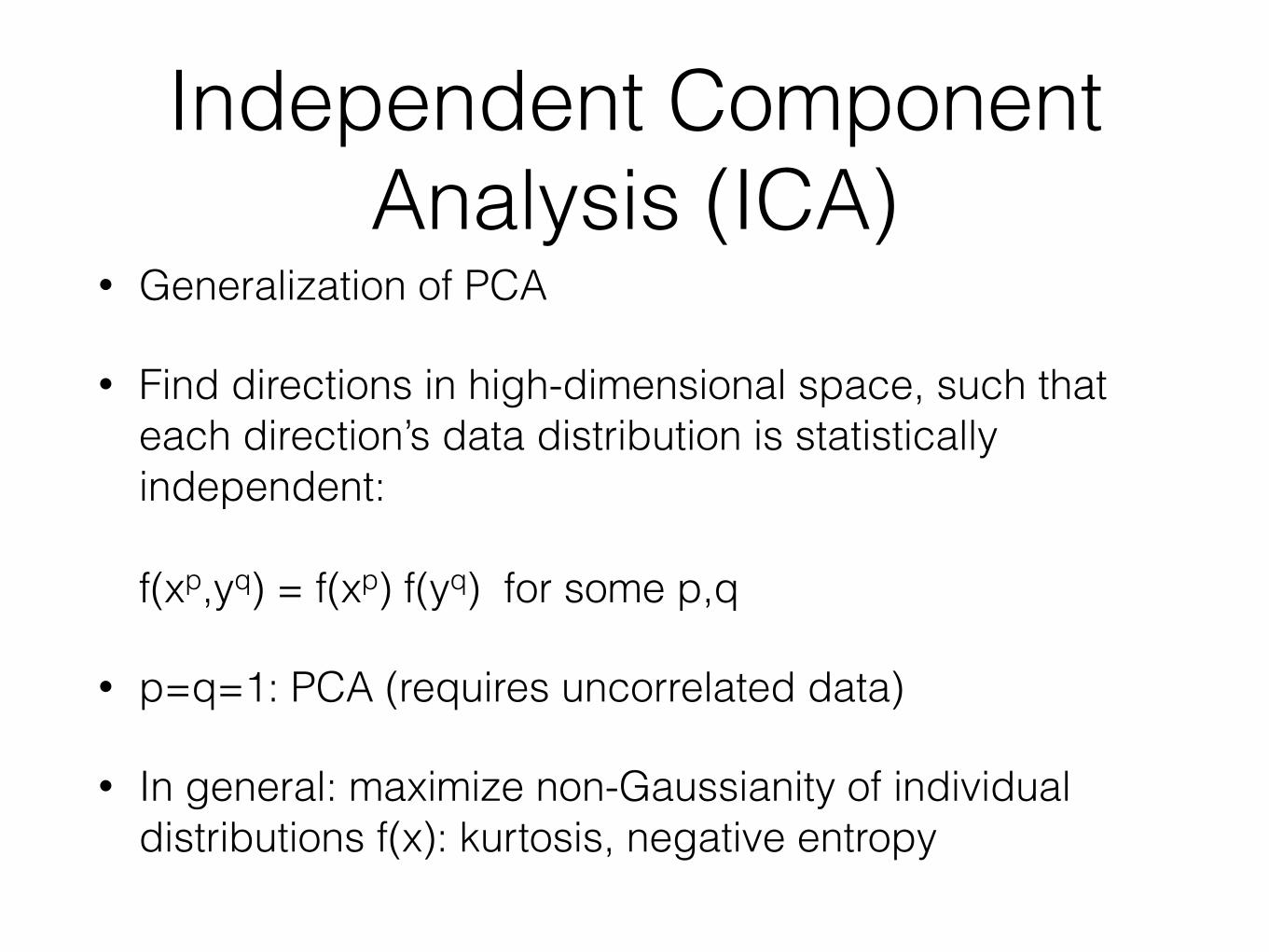
Independent Component Analysis (ICA)

• Generalization of PCA

• Find directions in high-dimensional space, such that each direction’s data distribution is statistically independent: f(xp,yq) = f(xp) f(yq) for some p,q

• p=q=1: PCA (requires uncorrelated data)

• In general: maximize non-Gaussianity of individual distributions f(x): kurtosis, negative entropy

ICA example: galaxy spectra in

SDSS


Other dimensionality reduction techniques

• Non-negative matrix factorization: similar to PCA/ICA, but components are always positive

• Manifold learning, e.g., locally-linear embedding: can deal with complex lower-dimensional objects in higher-dimensional space

• t-SNE: t-distributed stochastic neighbor embedding: models high-dimensional space as 2D in such a way that points close in high-D are close in 2D and points far are far in both

Regression

Regression problems• Have data set (x,y) —> y(x)?

• Issues: • y has errors with known Gaussian distribution, can be different • y has errors with known non-Gaussian distribution • y has unknown errors • x and y have known Gaussian errors • x and y have unknown errors

• Model complexity: • Linear —> relatively easy • Non-linear —> hard!

Regression: straight line• Model is y = mx +b

• Maximizing likelihood equivalent to solving: Y = A X, with YT = [y0,y1,…,yN-1], XT = [m,b], A = [[x0,1],[x1,1],…,[xN-1,1]]

• No errors: X = [ATA]-1ATY

• With errors: C = [[σ20,0,0,…,0],[0,σ21,0,…,0],…,[0,…,0,σ2N-1]]: X = [ATC-1A]-1ATC-1Y

• Prediction for xnew: [xnew,1] x [[ATC-1A]-1ATC-1Y]

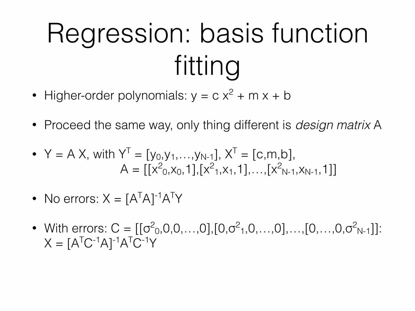
Regression: basis function fitting

• Higher-order polynomials: y = c x2 + m x + b

• Proceed the same way, only thing different is design matrix A

• Y = A X, with YT = [y0,y1,…,yN-1], XT = [c,m,b], A = [[x2

0,x0,1],[x21,x1,1],…,[x2

N-1,xN-1,1]]

• No errors: X = [ATA]-1ATY

• With errors: C = [[σ20,0,0,…,0],[0,σ2

1,0,…,0],…,[0,…,0,σ2N-1]]:

X = [ATC-1A]-1ATC-1Y

Regression: basis functions• Can use many more basis functions and approach non-parametric

regression

• E.g., Gaussian, piecewise-polynomial

• # of parameters grows —> need to penalize complexity

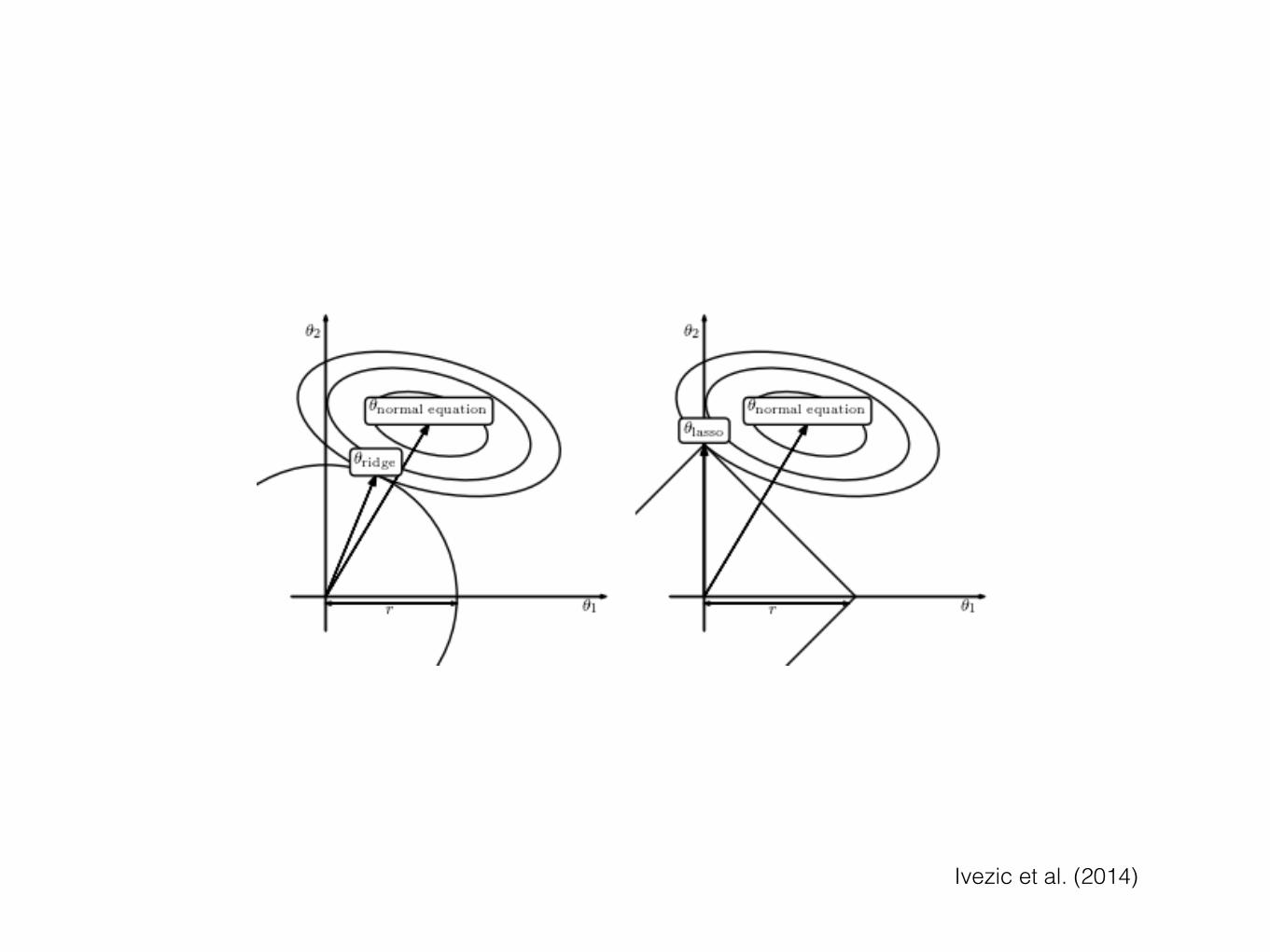
• Maximize: log L + regularization term

• regularization term: λ ∫dx|y’’(x)|2 —> spline λ |XTX| —> ridge regression λ |X| —> LASSO regression (prefers X = 0)

• Need to set λ —> cross-validation etc.

Basis function regression example


Gaussian Processes (GP)• Gaussian process is an example of an infinite-dimensional

model, sets a prior on functions

• GP: joint distribution of any [y(x0),y(x1),..,y(xN-1)] is Gaussian

• GP: characterized by mean function m(x) and covariance function Cov(x1,x2) that specify this joint distribution

• Mean and covariance function characterize by hyperparameters

• Magic of Gaussians make everything easy to deal with

• Need to choose Cov(x1,x2), popular choice is σ2 x exp(-(x1-x2)2/[2h2]) with parameters σ and h

• Can then draw functions from this Gaussian

Gaussian Processes (GP)


• If you have some observed data (xi,yi) with error bars, can write down the joint distribution of [x0,new,x1,new,…,xK-1,new,xi0,xi1,…,x1N-1]and condition on x0,new,x1,new,…,xK-1,new

• This gives the posterior distribution over functions, which is still Gaussian

Gaussian Processes (GP)

GP example

Rasmussen & Williams (2006)

GP math• Joint distribution

• Conditioning on observed points f


GP algorithm


Hyper-parameters

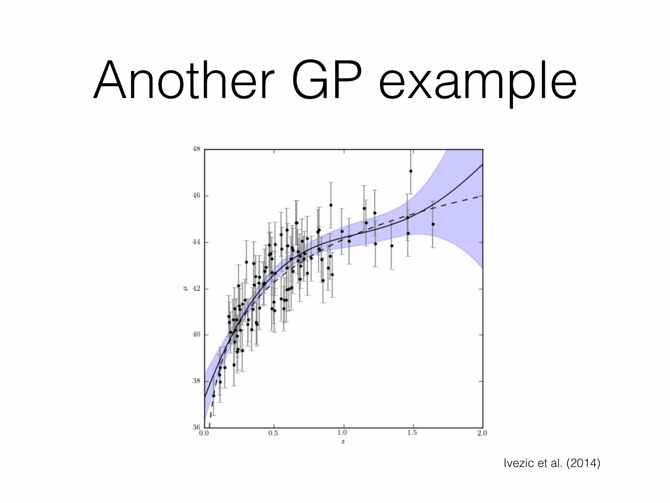
Another GP example


Classification

Classification• Example of supervised learning

• Have training data set of attributes xi with labels for K classes

• Learn how to assign labels based on attributes to classify unknown sources

• Example: (u,g,r,i,z) —> (quasar,star,galaxy)

Classification metrics

• Purity: fraction of objects assigned to class k that truly are part of class k

• Completeness: fraction of true class-k objects that is assigned to class k

• Difficult to maximize both!

Classification using density estimation

• Can estimate densities for each class ρk(x) = p(xnew|class k) using density-estimation techniques discussed earlier

• Assign new classes using Bayes theorem: p(xnew|class m) p(class m) p(class m|xnew) = ————————————— 𝛴k p(xnew|class k) p(class k)

• Allows for full power of density estimation

Example with Gaussian mixtures


Non-parametric classification: k-nearest neighbor

• Simple: Look at the k nearest neighbors in the training set —> assign class based on consensus

• Requires: • Distance function • Consensus building: can assign weights to

neighbors based on, e.g., the distance

• Expensive for large training sets (always need to consider all data)

Support Vector Machines• Find hyperplane in x that

maximizes the distance between two classes

• That hyperplane is entirely described by the points that lie on it —> support vectors

• Labels y={-1,1}, hyperplane:minimize |m| subject to yi(b+mxi) >= 1 for all i

• Can add loss function proportional to distance if data cannot be separated —> hyperparameter


SVM example


SVM: kernel trick• Hyperplane: linear

• Can make boundary non-linear using the kernel trick

• Requires the dual representation of the optimization problem for SVM…

• Replace all dot products with K(x,x’) with K a kernel (e.g., Gaussian)

SVM kernel trick example


Statistics and Inference -...

Documents

Transcript of Statistics and Inference -...