Statistics and Data Mining
35
Statistics & Data Mining Statistics & Data Mining R. Akerkar TMRF, Kolhapur, India Data Mining - R. Akerkar 1
-
Upload
rajendra-akerkar -
Category
Education
-
view
5.500 -
download
8
description
Transcript of Statistics and Data Mining

Statistics & Data MiningStatistics & Data Mining
R. AkerkarTMRF, Kolhapur, India
Data Mining - R. Akerkar 1

Why Data Preprocessing?
Data in the real world is dirtyy incomplete: lacking attribute values, lacking certain
attributes of interest, or containing only aggregate data e g occupation=“” e.g., occupation=
noisy: containing errors or outliers e.g., Salary=“-10”
inconsistent: containing discrepancies in codes or names e.g., Age=“42” Birthday=“03/07/1997” e.g., Was rating “1,2,3”, now rating “A, B, C” e.g., Was rating 1,2,3 , now rating A, B, C e.g., discrepancy between duplicate records
Thi i th l ld
Data Mining - R. Akerkar 2
This is the real world…

Why Is Data Dirty?y y Incomplete data comes from
/ n/a data value when collected different consideration between the time when the data was
collected and when it is analyzed. human/hardware/software problems
Noisy data comes from the process of dataC ll ti i t t’ f lt Collection instrument’s fault
Data entry transmission
Inconsistent data comes from Different data sources
F ti l d d i l ti
Data Mining - R. Akerkar 3
Functional dependency violation

Why Is Data Preprocessing Important?
No quality data no quality mining results! No quality data, no quality mining results! Quality decisions must be based on quality data
e.g., duplicate or missing data may cause incorrect or even g , p g ymisleading statistics.
Data warehouse needs consistent integration of quality data
Data extraction, cleaning, and transformation comprises the majority of the work of building a data warehouse Bill Inmonwarehouse. —Bill Inmon
Data Mining - R. Akerkar 4

Major Tasks in Data PreprocessingMajor Tasks in Data Preprocessing
Data cleaning Fill in missing values, smooth noisy data, and resolve
inconsistencies Data integration
Integration of multiple databases, data cubes, or files Data transformation
Normalization and aggregation ( a distance based mining algorithms Normalization and aggregation ( a distance based mining algorithms provide better results if data is normalized and scaled to range.)
Data reduction Obtains reduced representation in volume but produces the same or p p
similar analytical results (correlation analysis).
Data discretization Part of data reduction but with particular importance, especially for
Data Mining - R. Akerkar 5
p p p ynumerical data.

Forms of data preprocessingForms of data preprocessing
Data Mining - R. Akerkar 6
Data Cleaningg
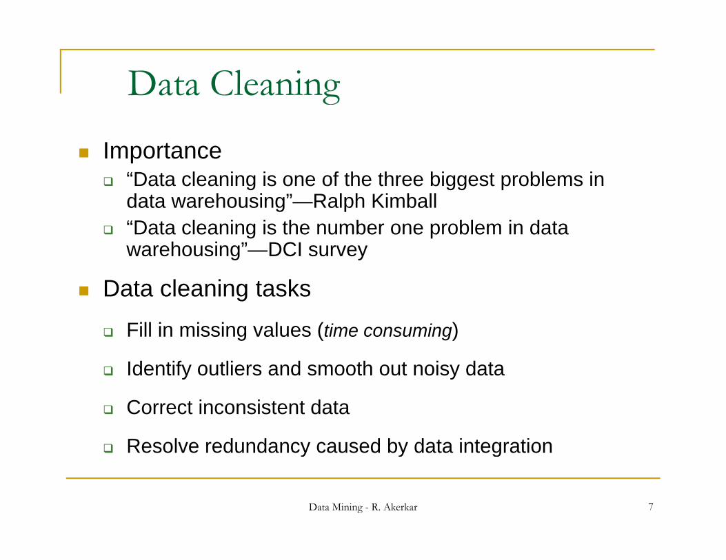
Importance“D t l i i f th th bi t bl i “Data cleaning is one of the three biggest problems in data warehousing”—Ralph Kimball
“Data cleaning is the number one problem in data h i ” DCIwarehousing”—DCI survey
Data cleaning tasks
Fill in missing values (time consuming)
Identify outliers and smooth out noisy data
Correct inconsistent data
Resolve redundancy caused by data integration
Data Mining - R. Akerkar 7
y y g

Missing Datag Data is not always available
E g many tuples have no recorded value for several attributes E.g., many tuples have no recorded value for several attributes, such as customer income in sales data
Missing data may be due to equipment malfunction
inconsistent with other recorded data and thus deleted
data not entered due to misunderstanding
certain data may not be considered important at the time of entryentry
not register history or changes of the data
Missing data may need to be inferred.
Data Mining - R. Akerkar 8
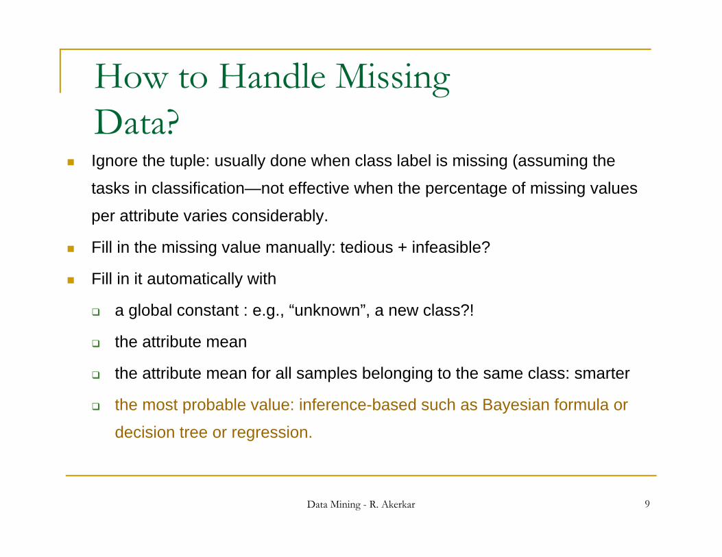
How to Handle Missing Data?
Ignore the tuple: usually done when class label is missing (assuming the
tasks in classification—not effective when the percentage of missing values
per attribute varies considerably.
Fill i th i i l ll t di + i f ibl ? Fill in the missing value manually: tedious + infeasible?
Fill in it automatically with
a global constant : e g “unknown” a new class?! a global constant : e.g., unknown , a new class?!
the attribute mean
the attribute mean for all samples belonging to the same class: smarter
the most probable value: inference-based such as Bayesian formula or
decision tree or regression.
Data Mining - R. Akerkar 9

Noisy Data
Noise: random error or variance in a measured variable.
For example, for a numeric attribute “price” how can we smooth out the data to remove the noise.
Incorrect attribute values may due to faulty data collection instruments data entry problems data transmission problems technology limitationgy inconsistency in naming convention
Data Mining - R. Akerkar 10

How to Handle Noisy Data?
Binning method: first sort data and partition into (equi-depth) bins then one can smooth by bin means, smooth by bin median,
smooth by bin boundaries etcsmooth by bin boundaries, etc.
Regressiong smooth by fitting the data into regression functions
Data Mining - R. Akerkar 11

Binning Methods for Data Smoothing* Binning methods smooth a sorted data by consulting its
neighborhood. Then sorted values are distributed in number of buckets.
* Sorted data for price (in dollars): 4, 8, 9, 15, 21, 21, 24, 25, 26, 28, 29, 34
* Partition into (equi-depth) bins of depth 4:- Bin 1: 4, 8, 9, 15- Bin 2: 21, 21, 24, 25- Bin 3: 26, 28, 29, 34
* Smoothing by bin means: Smoothing by bin means:- Bin 1: 9, 9, 9, 9- Bin 2: 23, 23, 23, 23- Bin 3: 29, 29, 29, 29
* S thi b bi b d i* Smoothing by bin boundaries:- Bin 1: 4, 4, 4, 15- Bin 2: 21, 21, 25, 25- Bin 3: 26, 26, 26, 34
Similarly, smoothing by bin median can be employed.
Data Mining - R. Akerkar 12
, , ,

Simple Discretization Methods: Binning
Equal-width (distance) partitioning:Di id th i t N i t l f l i Divides the range into N intervals of equal size: uniform grid
if A and B are the lowest and highest values of the gattribute, the width of intervals will be: W = (B –A)/N.
The most straightforward, but outliers may dominate presentationpresentation
Skewed data is not handled well.
Bi i i li d t h i di id l f t ( Binning is applied to each individual feature (or attribute). It does not use the class information.
Data Mining - R. Akerkar 13

Equal-depth (frequency) partitioning: Equal depth (frequency) partitioning: Divides the range into N intervals, each containing
approximately same number of samples Good data scaling Managing categorical attributes can be tricky.
Data Mining - R. Akerkar 14
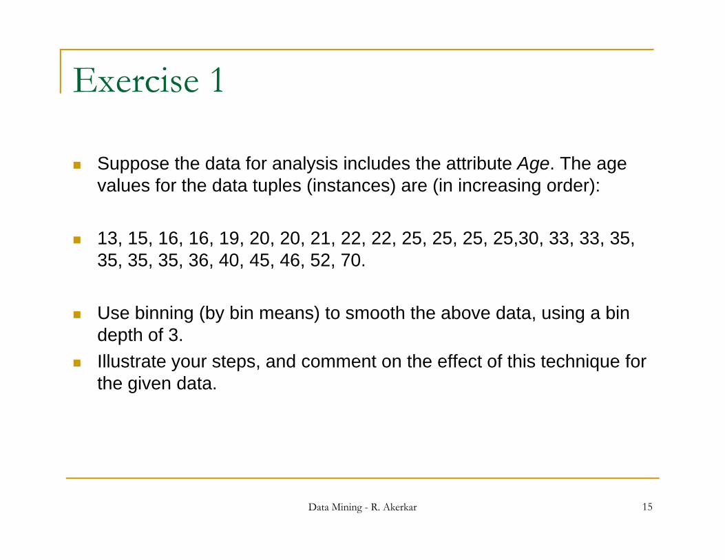
Exercise 1
Suppose the data for analysis includes the attribute Age. The age values for the data tuples (instances) are (in increasing order):
13, 15, 16, 16, 19, 20, 20, 21, 22, 22, 25, 25, 25, 25,30, 33, 33, 35, , , , , , , , , , , , , , , , , , ,35, 35, 35, 36, 40, 45, 46, 52, 70.
Use binning (by bin means) to smooth the above data using a bin Use binning (by bin means) to smooth the above data, using a bin depth of 3.
Illustrate your steps, and comment on the effect of this technique for the given datathe given data.
Data Mining - R. Akerkar 15

Data Integrationg Data integration:
combines data from multiple sources into a coherent store combines data from multiple sources into a coherent store
Schema integrationE tit id tifi ti bl id tif l ld titi f Entity identification problem: identify real world entities from multiple data sources, e.g., A.cust-id B.cust-#
integrate metadata from different sources
Detecting and resolving data value conflicts for the same real world entity, attribute values from different
so rces are differentsources are different possible reasons: different representations, different scales,
e.g., metric vs. British units
Data Mining - R. Akerkar 16

Handling Redundancy in Data Integration
Redundant data occur often when integration of multiple databases The same attribute may have different names in different
databases One attribute may be a “derived” attribute in another table e g One attribute may be a derived attribute in another table, e.g.,
annual revenue Redundant data may be able to be detected by correlation analysis Careful integration of the data from multiple sources may help
reduce/avoid redundancies and inconsistencies and improve mining speed and quality
Data Mining - R. Akerkar 17
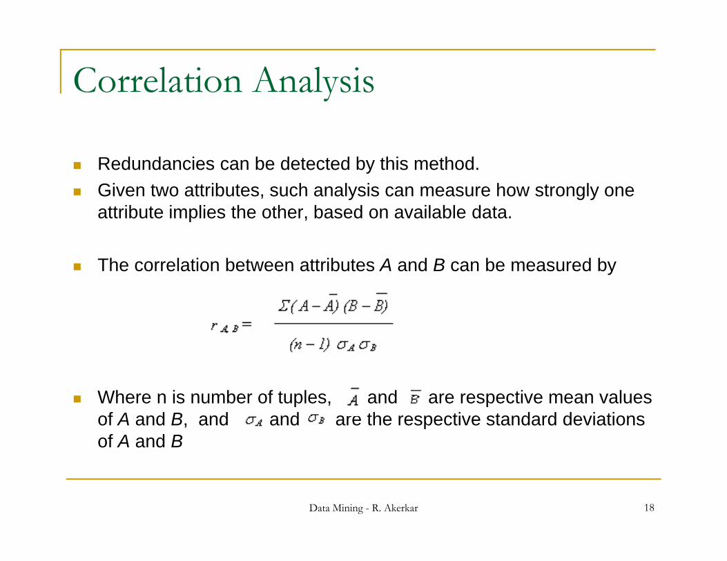
Correlation Analysis
Redundancies can be detected by this method. Given two attributes, such analysis can measure how strongly one
attribute implies the other, based on available data.
The correlation between attributes A and B can be measured by
Where n is number of tuples, and are respective mean values of A and B, and and are the respective standard deviations of A and B
Data Mining - R. Akerkar 18
Correlation Analysis If the resulting value of the equation is greater than 0, then A and B
are positively correlated. i th l f A i th l f B i i.e. the values of A increase as the values of B increase.
The higher the value, the more each attribute implies the other. Hence, high value may indicate that A (or B) may be removed as
redundancyredundancy.
If the resulting value is equal to zero, then A and B are independent There is no correlation between them.
If the resulting value is less than zero, then A and B are negatively correlated. i.e. the values of one attribute increase as the values of other attribute
decrease. Each attribute discourages the other.
Data Mining - R. Akerkar 19

Correlation Analysis
Above are three possible relationships between data. The graphs of high positive and negative correlation are approaching a value of 1 and -1 respectively. The graph showing no correlation has a value of 0.
Data Mining - R. Akerkar 20
Categorical Data
To find the correlation between two categorical attributes we make use of contingency tables.g y
Let us consider the following: Let there be 4 car manufacturers given by the set Let there be 4 car manufacturers given by the set
{A,B,C,D} and let there be three segments of cars manufactured by these companies given by the set {S M L} where S stands for small cars M stands for{S,M,L}, where S stands for small cars, M stands for medium sized cars and L stands for Large cars.
Observer collects data about the cars passing by, manufactured by these companies and categorize them according to their sizes.
Data Mining - R. Akerkar 21
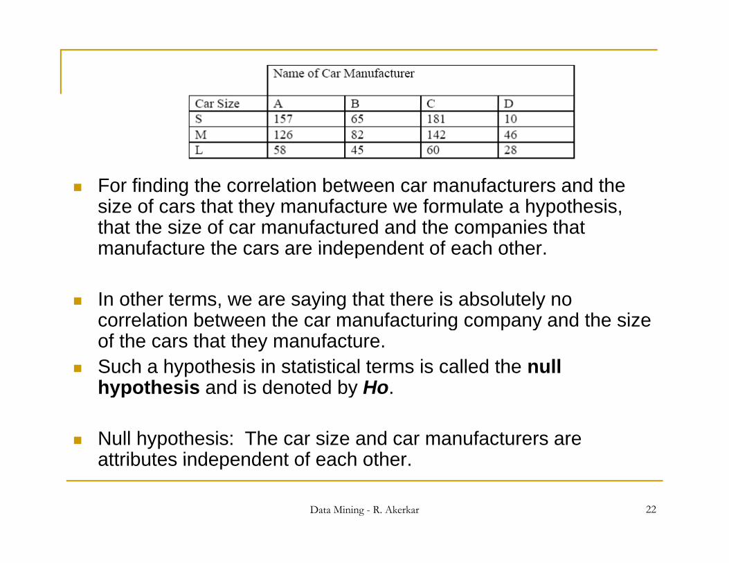
For finding the correlation between car manufacturers and the size of cars that they manufacture we formulate a hypothesis, that the size of car manufactured and the companies that manufacture the cars are independent of each othermanufacture the cars are independent of each other.
In other terms, we are saying that there is absolutely no correlation between the car manufacturing company and the sizecorrelation between the car manufacturing company and the size of the cars that they manufacture.
Such a hypothesis in statistical terms is called the null hypothesis and is denoted by Hohypothesis and is denoted by Ho.
Null hypothesis: The car size and car manufacturers are attributes independent of each other
Data Mining - R. Akerkar 22
attributes independent of each other.
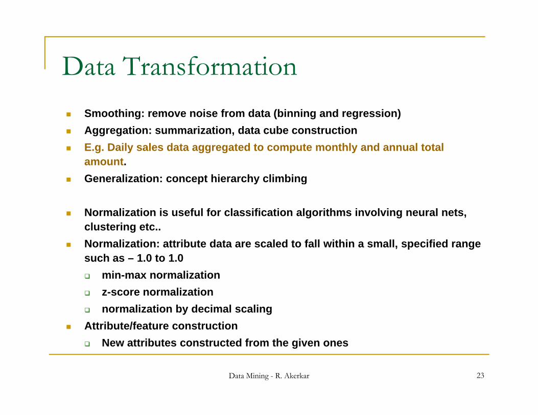
Data Transformation Smoothing: remove noise from data (binning and regression)
Aggregation: summarization data cube construction Aggregation: summarization, data cube construction E.g. Daily sales data aggregated to compute monthly and annual total
amount. Generalization: concept hierarchy climbing Generalization: concept hierarchy climbing
Normalization is useful for classification algorithms involving neural nets, clustering etc..
Normalization: attribute data are scaled to fall within a small, specified range such as – 1.0 to 1.0 min-max normalization z-score normalization normalization by decimal scaling
Attribute/feature constructionf
Data Mining - R. Akerkar 23
New attributes constructed from the given ones

Data Transformation: Normalization min-max normalization (This type of normalization transforms the data into a
desired range, usually [0,1]. )
AAA
AA
A minnewminnewmaxnewminmax
minvv _)__('
where, [minA, maxA] is the initial range and [new minA, new maxA] is the , [ , ] g [ _ , _ ]new range.
e.g.: If v = 73600 in [12000, 98000] Then v’ = 0.716 in the range [0, 1].
Here value for “income” is transformed to 0.716
It th l ti hi th i i l d t l
Data Mining - R. Akerkar 24
It preserves the relationship among the original data values.
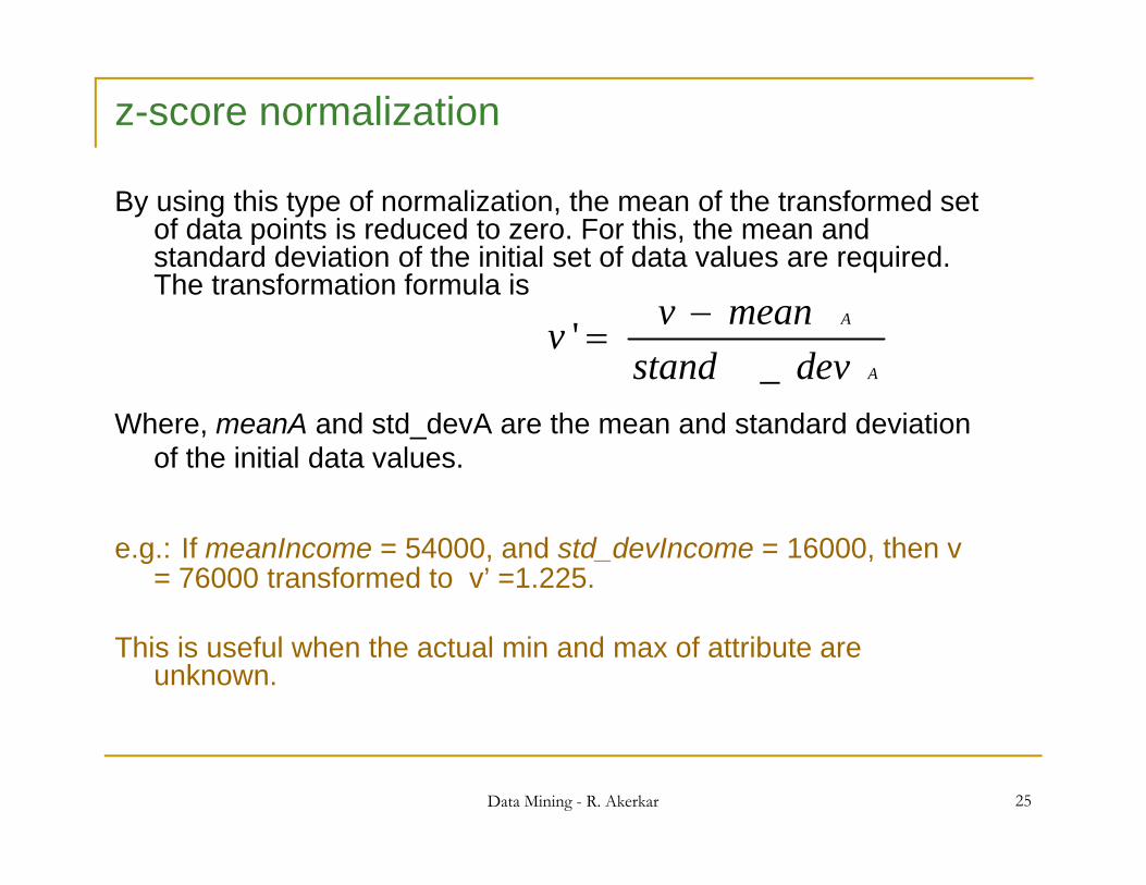
z-score normalization
By using this type of normalization, the mean of the transformed set of data points is reduced to zero. For this, the mean and standard deviation of the initial set of data values are required. Th t f ti f l iThe transformation formula is
A
A
devstandmeanvv
_'
Where, meanA and std_devA are the mean and standard deviation of the initial data values.
_
e.g.: If meanIncome = 54000, and std_devIncome = 16000, then v = 76000 transformed to v’ =1.225.
This is useful when the actual min and max of attribute are unknown.
Data Mining - R. Akerkar 25
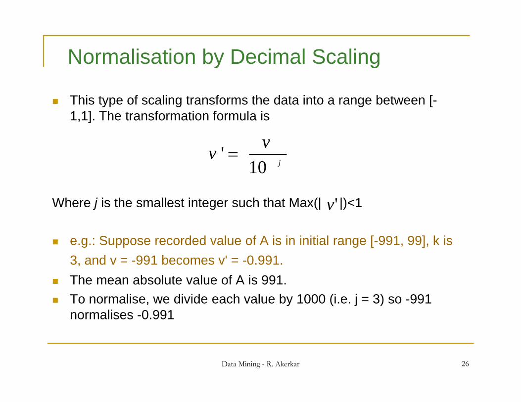
Normalisation by Decimal Scaling
This type of scaling transforms the data into a range between [-1,1]. The transformation formula is
j
vv10
'
Where j is the smallest integer such that Max(| |)<1'v
e.g.: Suppose recorded value of A is in initial range [-991, 99], k is 3, and v = -991 becomes v' = -0.991.Th b l t l f A i 991 The mean absolute value of A is 991.
To normalise, we divide each value by 1000 (i.e. j = 3) so -991 normalises -0.991
Data Mining - R. Akerkar 26

Exercise 2
Using the data for Age in previous Question, answer the following:
a) Use min-max normalization to transform the value 35 for age into the range [0.0; 1.0].
b) Use z-score normalization to transform the value 35 for age, where the standard deviation of age is 12.94.
c) Use normalization by decimal scaling to transform the value 35 for age.
d) Comment on which method you would prefer to use for the givend) Comment on which method you would prefer to use for the given data, giving reasons as to why.
Data Mining - R. Akerkar 27
What Is Prediction?What Is Prediction?
Prediction is similar to classification Prediction is similar to classification First, construct a model Second, use model to predict unknown value
Major method for prediction is regression Major method for prediction is regression Linear and multiple regression Non-linear regression
P di ti i diff t f l ifi ti Prediction is different from classification Classification refers to predict categorical class label Prediction models continuous-valued functions
E.g. A model to predict the salary of university graduate with 15 years of work experience.
Data Mining - R. Akerkar 28

Regression
Regression shows a relationship between the average values of two variables.
Thus regression is very useful in estimating and predicting the average value of one variable for a given value of other variable.
The estimate or prediction may be made with the help of a regression line.
There are two types of variables in regression analysis-independent variable and dependent variable.
The variable whose value is to be predicted is called dependent i bl d th i bl h l i d f di ti ivariable and the variable whose value is used for prediction is
called independent variable.
Data Mining - R. Akerkar 29

Linear regression: If the regression curve is a straight g g gline, then there is a linear regression between two variables.
Linear regression models a random variable Y (called Linear regression models a random variable, Y (called response variable) as a linear function of another random variable, X ( called a predictor variable)
Y = + X Y = + X Two parameters , and specify the line and are to
be estimated by using the data at hand. (regression coefficients)
The variance of Y is assumed to be constant. Th ffi i t b l d f b th th d f The coefficients can be solved for by the method of least squares (minimizes the error between the actual data and the estimate of the line. )
Data Mining - R. Akerkar 30
)

Linear Regression
Given s samples or data points of the form (x1, y1), (x2, y2) …(xs, ys) The regression coefficients can be estimated as,
Where is the average of x1, x2 … and is the average of y1, y2,…
Data Mining - R. Akerkar 31
Multiple Regression
Multiple regression: Y = + 1 X1 + 2 X2.p g 1 1 2 2
Many nonlinear functions can be transformed into the above.
The regression analysis for studying more than two variables at a timetwo variables at a time.
It involves more than one predictor variable. Method of least square can be applied to solve for Method of least square can be applied to solve for
, 1, and 2.
Data Mining - R. Akerkar 32

Non-Linear Regression
If the curve of regression is not a straight line, i.e., a first degree equation in the variables x and y, then it is called a non-linear regression or curvilinear regression
Consider a cubic polynomial relationship, Y = + 1X + 2X2 + 3X3.
To convert above equation in linear form, we define new variable: To convert above equation in linear form, we define new variable: X1 = X, X2 = X2, X3 = X3
Thus we get,g Y = + 1X1 + 2 X2+ 3 X3.
This is solvable by the method of least squares
Data Mining - R. Akerkar 33
This is solvable by the method of least squares.

Exercise 3
Following table shows a set of X Ypaired data where X is the number of years of work experience of a college graduates and Y is the corresponding salary of the
Years Experience Salary (in $ 1000s)
3 30
8 57
9 64corresponding salary of the graduate.
Draw a graph of the data. Do X and Y seem to have a linear
9 64
13 72
3 36
6 43relationship? Also, predict the salary of a
college graduate with 10 years of experience
6 43
11 59
21 90
1 20experience. 16 83
Data Mining - R. Akerkar 34

Assignment
The following table shows the midterm and
XMidterm exam
YFinal exam
72 84
final exam grades obtained for students in a data mining course.
50 63
81 77
74 78
1. Plot the data. Do X and Y seem to have a linear relationship?
2. Use the method of least squares to find an equation for the prediction of a student’s
94 90
86 75
59 49
83 79equation for the prediction of a student s final grade based on the student’s midterm grade in the course.
3. Predict the final grade of a student who
83 79
65 77
33 52
88 74greceived an 86 on the midterm exam.
88 74
81 90
Data Mining - R. Akerkar 35