Statistics

1

Statistics

Achim TreschGene CenterLMU Munich

2

Topics

I. Descriptive Statistics

II. Test theory

III. Common tests

IV. Bivariate Analysis

V. Regression

3

III. Common Tests

…Gene A

Gene B

Gene expressionmeasurements

Which gene is„differentially“ expressed?

Group 1Group 2

Two group comparisons

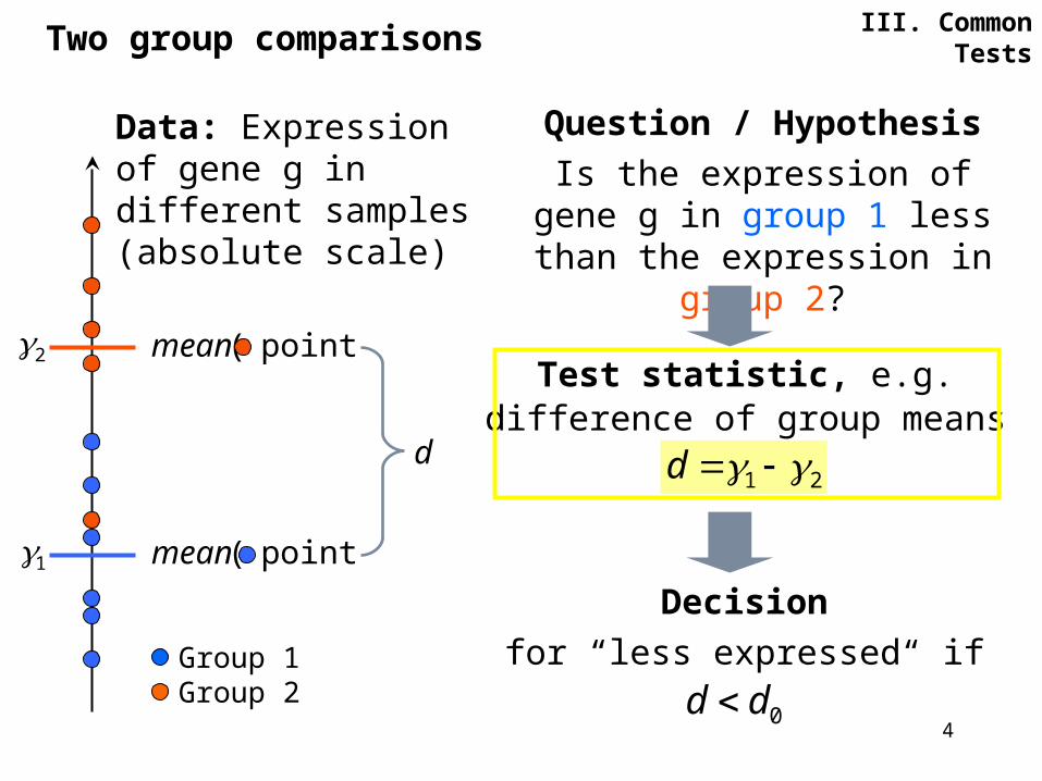
4

Group 1Group 2

points) ( mean

Question / HypothesisIs the expression of gene g

in group 1 less than the expression in group 2?

Data: Expression of gene g in different samples (absolute scale)

points) ( mean

2

1Decision

for “less expressed“ if

0dd

d

Test statistic, e.g.difference of group means

21 d

III. Common TestsTwo group comparisons

5

Bad Idea: Subtract the group means

21 d

2

1

d

2

d

Problem: d is not scale invariant

1

)( ds

dt

Solution:Divide d by its standard

deviation

This is essentially the two sample t-statistic (for unpaired samples)

Group 1Group 2

III. Common TestsTwo group comparisons

6

There are variants of the t-test:

One group:one sample t-test (is the group mean = μ ?)

with mean and variance

Two group comparisons:Paired t-test (are the group means equal ?) -> latertwo sample t-test assuming equal variancestwo sample t-test not assuming equal variances

(Baum-Welch test)

III. Common TestsThe t-test

x

t

2

22

1

21

21

nn

xxt

n

jjxx

1

n

jj xx

n 1

2)(1

1

7

Requirement: The data is approx. normally distributed in both groups (there are ways to check this, e.g. by the Kolmogoroff-Smirnov test)

III. Common TestsThe t-test

Decision for unpaired t-test or Baum-Welch test:

8

Wilcoxon rank sum test (Mann-Whitney-Test, U-test)

Non parametric test for the comparison of two groups: Is the distribution in group 1 systematically shifted relative to group 2 ? Data

Group 1 18 3 6 9 5

Group 2 15 10 8 7 12

1 2 3 4 5 6 7 8 9 10

3 5 6 7 8 9 10 12 15 18 Original

scaleRank scale

Rank sum Group 1: 1+2+3+6+10 = 22

Rank sum Group 2:4+5+7+8+9 = 33

III. Common Tests

9

The test statistic is the rank sum of group 1

Rank sum distribution for group 1, |Group 1| = 5, |Group 2| = 5

The corrseponding p-value can be calculated exactly for small group sizes. There are approximations available for larger group sizes (N>20).

22

P(W≤22, H0) = 0.15

Wilcoxon W

15 20 25 30 35 40

III. Common Tests

The Wilcoxon test can be carried out as a one-sided and as a two-sided test (default)

Wilcoxon rank sum test (Mann-Whitney-Test, U-test)

10

Reminder paired data: There are coupled measurements (xi, yi) of the same kind.

x1, x2, ....., xn

Data

y1, y2, ....., yn

Essential: Calculate the differences of the pairsd1 = x1 – y1, d2 = x2 – y2,..... dn = xn – yn.

Now perform a one-sample t-test for the data (dj) with μ=0.

Advantage over unpaired data: Removal of „interindividual“ = intra group variance

Tests for paired samplesIII. Common Tests

NB: Approx. normal distribution of the data in both groups is a requirement.

11

ohne autogenes Training mit autogenem Training

40

50

60

70

80

Pulsfrequenz

Differenz

-5

-2,5

0

2,5

5

7,5

10

Pulsfrequenz

t-Test for paired samples

Graphical Description:

Difference Boxplot

III. Common Tests

pulse pulse

untrained trained Difference

12

Wilcoxon signed rank test

Nonparametric version for paired samples:Are the values in group 1 smaller than in group 2 ?

Data

Group 1 18 3 6 9 5

Group 2 15 10 8 7 12

Difference Gr.2-Gr.1 -3 7 2 -2 7

Idea: If the groups are not different, the „mirrored“ distribution of the differences with a negative sign should be similar to the distribution of the differences with a positive sign.Check similarity with a Wilcoxon rank sum test for the comparison of -∎ und ∎ .

III. Common Tests

13

0 1 2 3 4 5 6 7 8 9 . . .

-3 -2 2 7Original scaleAbsolute values

Rank sums: Group 1: 1.5+3 = 4.5 Group 2: 1.5+4.5+4.5 = 10.5

Negative Differences

Positive Differences

Rank scale* 1 2 3 4 5 6 . . .

→ Perform a Wilcoxon rank sum test for |Gruppe 1| = 2 , |Gruppe 2| = 3

* In case of k ties (k identical values), replace the ranks j,…,j+k-1 of these by the common value j + (k-1)/2.

Wilcoxon signed rank testIII. Common Tests

14

Summary: Group comparison of a continuous endpoint

Does the data follow a Gaussian

distribution?

Paired data? Paired data?

t-Test for paired data

yes no

t-Test for unpaired data

Wilcoxon signed rank test

Wilcoxon rank sum test

ja janein

nein

Question: Are group 1 and group 2 identical with respect to the distribution of the endpoint?

III. Common Tests

15

Var. Y

0 1 ∑

Var. X

0 a b a+b

1 c d c+d

∑ a+c b+cN=

a+b+c+d

Comparison of two binary variablesunpaired data: Fisher‘s Exact Test

III. Common Tests

given

ca

N

c

dc

a

ba

db,ca,b,c,d|a )P(

) than"extreme more is" /B

A P( p db,c|a

bc

ad

D

C

Are there differences in the distribution █ and █ ?

16

Effect of Placebo

yes no

Effect of

Verum

yes 31 15

no 2 14

Are the measurements in █ resp. █ concordant or discordant?

Concordant pairs

Discordant pairs

Comparison of two binary variables Paired data: McNemar Test („sparse Scotsman“)

Ex.: Clinical trial, Placebo vs. Verum (each individual obtains both treatments at different occasions)

III. Common Tests

17

Are the measurements in █ resp. █ concordant or discordant?

Comparison of two binary variables Paired data: McNemar Test („Sparsamer Schotte“)

III. Common Tests

Var. X, measurement 2

0 1 ∑

Var. X, mea-sure-

ment 1

0 a b a+b

1 c d c+d

∑ a+c b+cN=

a+b+c+d

cb

cb

2

2 )5.0|(|

)|| |C-B| P( p cbcb

18

H0: The two variables are independent.

Comparison of two categorial variablesUnpaired data Stichproben: Chisquared-Test (χ2-Test)

III. Common Tests

Var. Y

0 1 … s ∑

Var. X

0 n00 n01 n0.

1 n10 n11 n1.

… njk

r nr.

∑ n.1 n.2 n.s N

N

n

N

nNPNPN kjkj

....jk

jk )()()P(N

n

Idea: Measure deviation from this equality

r

j

s

k kj

kj

nn

nn

1 1 ..

2..jk2

/N

/N)-(n

This test statistic follows asymptotically a χ2-distribution. -> Requirement: each cell contains ≥ ~5 counts.

19

Binary data?

Paired data? Paired data?

McNemar Test

yes no

Fisher‘s Exact Test

(bivariate symmetry

tests)

Chisquared (χ2) -test

yes yesno no

Question: Is there a difference in the frequency distributions of one variable w.r.t. the values of the second variable?

Summary: Comparison of two categorial variablesIII. Common Tests

20

Summary Description and Testing(Two sample comparison)

variable Design Deskription numerisch

Deskription graphisch

Test

continuous

unpaired

continuous

paired

binary unpaired

binary paired

categorial unpaired

* For Gaussian distributions/ at least: symmetric distributions (|skewness|<1)

III. Common Tests

21




Test

continuous

unpairedMedian, Quartile

2 BoxplotsWilcoxon-rank sum-/

unpaired t-Test*

continuous

paired

binary unpaired

binary paired

categorial unpaired


III. Common Tests

22




Test

continuous



unpaired t-Test*

continuous

pairedMedian,

Quartile of difference

Difference-Boxplot

Wilcoxonsigned rank-/paired t-Test*

binary unpaired

binary paired

categorial unpaired


III. Common Tests

23




Test

continuous



unpaired t-Test*

continuous

pairedMedian,


Difference-Boxplot


binary unpairedCross table,

row%(3D-)Barplo

tFisher‘s Exact

Test

binary paired

categorial unpaired


III. Common Tests

24




Test

continuous



unpaired t-Test*

continuous

pairedMedian,


Difference-Boxplot



row%(3D-)Barplo

tFisher‘s Exact

Test

binary paired

Cross table (“Mc-

Nemar-table“)

(3D-)Barplot

McNemar-Test

categorial unpaired


III. Common Tests

25




Test

continuous



unpaired t-Test*

continuous

pairedMedian,


Difference-Boxplot



row%(3D-)Barplo

tFisher‘s Exact

Test

binary paired

Cross table (“Mc-

Nemar-table“)

(3D-)Barplot

McNemar-Test

categorial unpairedCross table,

row%(3D-)Barplo

tχ2-Test


III. Common Tests

26

Caveat:

For large sample numbers, very small differences may become significant

For small sample numbers, an observed difference may be relevant, but not statistically significant

Statistical Significance ≠ Relevance

III. Common Tests

27

Examples:

Simultaneous testing of many endpoints (e.g. genes in a microarray study)

Simultaneous pairwise comparison of many (k) groups (k pairwise tests = k(k-1)/2 tests)

Although each individual test keeps the significance level (say α = 5%), the probability of obtaining (at least one) false positive increases dramatically with the number of tests:For 6 tests, the probability of a false positive is already >30%! (if there are no true positives)

Multiple Testing ProblemsIII. Common Tests

28

One possible solution: p-value correction for multiple testing, e.g. Bonferroni correction:Each single test is performed at the level α/m („local significance level α/m“), where m is the number of tests.The probability of obtaining a (at least one) false positive is then at most α („multiple/global significance level α“) Ex.: m = 6

Desired multiple level: α = 5%

→ local level: α/m = 5%/6 = 0.83%

III. Common Tests

Multiple Testing Problems

Other solutions: Bonferroni-Holm, Benjamini-Hochberg,Control of False discovery rate (FDR) instead of significance at the group level (family wise error rate, FWER): SAM

29

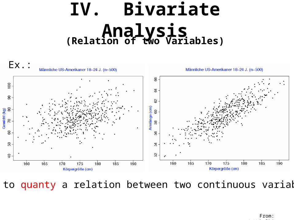
IV. Bivariate Analysis(Relation of two Variables)

From: A.Wakolbinger

How to quanty a relation between two continuous variables?

Ex.:

30

Pearson-Correlation coefficient rxy

Useful for gaussian variables X,Y (but not only for those)Measures the degree of linear dependence


Properties: -1 ≤ rxy ≤ +1

rxy = ± 1: perfect linear dependence

The sign indicates the direction of the relation (pos/neg dependence)

From: A.Wakolbinger

31

The closer rxy to 0, the weaker the (linear) dependence

From: A.Wakolbinger



32

From: A.Wakolbinger




33

From: A.Wakolbinger




34

From: A.Wakolbinger




35

From: A.Wakolbinger




36

rxy = ryx (Symmetry)

From: A.Wakolbinger




37

rxy = 0,38 rxy = 0,84

Example: Relation body height – body weight – arm length

The closer the data scatters around the regression line (see later), the larger |rxy|.

From: A.Wakolbinger



38

How large is r in these examples?

rxy ≈ 0

The Pearson correlation coefficient cannot measure non-linear dependence properly.

rxy ≈ 0

rxy ≈ 0



39

Spearman correlation sxy

X

Y

Rang(X)

Ra

ng

(Y)

Idea: Calculate the Pearson correlation coefficient on rank transformed data.

X

Y

Rang(Y

)

Rang(X)

Spearman correlation measures the monotony of a dependence.

rxy = 0,88 sxy = 0,95


40

Pearson vs. Spearman correlationO

rigin

al sc

ale


41

Pearson correlation

NM_001767NM_001767 NM_000734NM_000734 NM_001049NM_001049 NM_006205NM_006205

NM_001767NM_001767 1.00000000 0.94918522 -0.04559766 0.04341766

NM_000734NM_000734 0.94918522 1.00000000 -0.02659545 0.01229839

NM_001049NM_001049 -0.04559766 -0.02659545 1.00000000 -0.85043885

NM_006205NM_006205 0.04341766 0.01229839 -0.85043885 1.00000000

Pearson vs. Spearman correlationIV. Bivariate Analysis

42

Ran

k tr

ansf

orm

ed d

ata


43

NM_001767NM_001767 NM_000734NM_000734 NM_001049NM_001049 NM_006205NM_006205

NM_001767NM_001767 1.00000000 0.9529094 -0.10869080 -0.17821449

NM_000734NM_000734 0.9529094 1.00000000 -0.11247013 -0.20515650

NM_001049NM_001049 -0.10869080 -0.11247013 1.00000000 0.03386758

NM_006205NM_006205 -0.17821449 -0.20515650 0.03386758 1.00000000

Spearman correlation


44

Conclusion: Spearman correlation is more robust against outliers and insensitive against changes of scale. In case of a (expected) linear dependence however, Pearson correlation is more sensitive.


45

Summary

Pearson correlation is a measure for linear dependence

Spearman correlation is a measure for monotone dependence

Correlation coefficients do not tell anything about the (non-)existence of a functional dependence.

Correlation coefficients tell nothing about causal relations of two variables X and Y (on the contrary, they are symmetric in X and Y)

Correlation coefficients hardly tell anything about the shape of a scatterplot


46

Foot size

Inco

me

Foot size Incomecorr.

Gender

Example:

Fake correlation, Confounding

Confounding: A variable that „explains“ (part of) the dependence of two others.

r=0.6


47

Partial correlation: = „remaining “ correlation(here: after correction w.r.t. gender)

rXY | Geschl. = partial correlation =

2

rxy ( ) + rxy ( )

Foot size

Inco

me r=0.03

Difference due to sex = Mean(Inc.♂) - Mean(Inc.♀)

Fake correlation, ConfoundingIV. Bivariate Analysis

48

V. Regression(Approximation of one variable by

a function of a second variable)

Unknown functional

dependence

Population

$

$

$

$$ $$

$$ $$

Sample

$$ $$

iii XfY )( iii XfY )(Regression

function

49

V. Regression

Choose a family of functions that you think is capable of capturing the functional dependence of the two variables.E.g. the set of linear functions, f(x) = ax+b or the set of quadratic functions, f(x) = ax2+bx+c

Regression: The Method

0

50

100

0 20 40 60

50

0204060

0 20 40 60

X

Y

Regression: The Method

Choose a loss function = the quality measure for the approximation. E.g. for continuous data usually: Quadratic Loss (RSS, Residual Sum of Squares)

Y= f(X)

RSS = Σj(actual value – predicted value) 2

= Σj( Yj- f(Xj) )2

f(Xj)

Prediction

Yj

Xj

(Xj ,Yj)Actual value

Residual

V. Regression

51

Identify the (a) function from the family of candidates that approximates the response variable best in terms of the loss function.

Regression: Methode

0

50

100

0 20 40 60

RSS = 1.1

RSS = 3

RSS = 1.7

RSS = 8.0

V. Regression

52

Univariate linear Regression

Bra

in w

eig

ht

Body weight

V. Regression

Brain weight as a function of body weight

Brain-/Body weights of 62 mammals

53


Log

10(B

rain

weig

ht)

Log10(Body weight)

V. Regression



http://images.google.de/imgres?imgurl=http://www.schiefer.de/images/pressemitteilungen/2003/Sendung_mit_der_Maus/Bild_3.jpg&imgrefurl=http://mschiefner.blogschrift.org/categories/6-Studien&h=448&w=319&sz=66&hl=de&start=1&um=1&tbnid=5qZyP0BhLnv5gM:&tbnh=127&tbnw=90&prev=/images%3Fq%3Ddie%2Bsendung%2Bmit%2Bder%2Bmaus%26svnum%3D10%26um%3D1%26hl%3Dde%26sa%3DG

54


Log

10(G

ehir

ngew

icht)

Log10(Körpergewicht)

V. Regression



55

Chironectes minimus (Schwimmbeutelratte, Wasseropossum)


Log

10(G

ehir

ngew

icht)

Residuen

Log10(Körpergewicht)

V. Regression


Residuals

56

One possible measure: coefficient of determination, R2

Measures the fraction of the variance that is not explained away by the regression function:

R2 = 1 – unexplained Var. / total Var. = 1 - RSS/Var(Y)

If we were using linear regression, R2 is simply the squared Pearson correlation of X and Y:

R2 = rxy2

(and hence 0 ≤ R2 ≤ 1)

Goodness of Fit, Model selectionQuestions:

Did I choose a proper class of approximation functions („a good regression model“)?How good does my regression function fit the data?

V. Regression

57

II.10 Gütekriterien

Questions?

58

Der Zufall ist ein Pseudonym, das der liebe Gott wählt, wenn er unerkannt bleiben will.

Albert Schweitzer

Schönheit ist die Abwesenheit von Zufällen.

Felix Magath

Ein Kasten Bier hat 24 Flaschen, ein Tag hat 24 Stunden. Das kann doch kein Zufall sein.

Anonymus

Was ist Zufall?

http://turnbull.mcs.st-and.ac.uk/history/Mathematicians/Kolmogorov.html

59

End of Part II

Statistics

Documents

Transcript of Statistics