Statistics 2000, Section 001, Final (300 Points)

Wednesday, December 15, 2010

Part I: Text Answers

Your Name:

Question 1: Statistical Inference (50 Points)

A lab scientist is interested in whether lab rats that grow up alone grow as large as labrats that grow up with other rats around them to play with. He randomly selects tenyoung rats with approximately the same age and size. Five of these will spend the next 4months by themselves and the other five rats will each have three other rats to play withduring that same time. After 4 months, the scientist measures the abdomen circumferenceof all the rats (in mm). The results are shown below:

The sample means and sample standard deviations are: x1 = 113.8 and s1 = 7.98,x2 = 127.8 and s2 = 6.38. It is reasonable to believe that rat weights in each grouproughly follow a normal distribution. Show your work!

1. (8 Points) What are the hypotheses to test whether the rats grow up to be equallylarge or whether the playing rats grow up larger? Use the proper mathematicalnotation and symbols.

2. (4 Points) Briefly justify your choice of a one-sided or two-sided alternative in theprevious part.

1

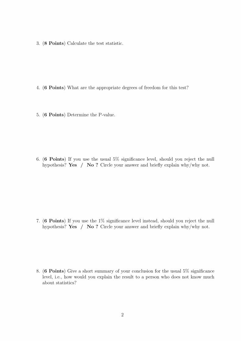
3. (8 Points) Calculate the test statistic.

4. (6 Points) What are the appropriate degrees of freedom for this test?

5. (6 Points) Determine the P-value.

6. (6 Points) If you use the usual 5% significance level, should you reject the nullhypothesis? Yes / No ? Circle your answer and briefly explain why/why not.

7. (6 Points) If you use the 1% significance level instead, should you reject the nullhypothesis? Yes / No ? Circle your answer and briefly explain why/why not.

8. (6 Points) Give a short summary of your conclusion for the usual 5% significancelevel, i.e., how would you explain the result to a person who does not know muchabout statistics?

2

Question 2: Regression (40 Points)

Before Thanksgiving, a supermarket ran the following ad regarding their turkey sale:

Scatterplot of the data:

●

●

●

●

●

10 11 12 13 14 15

0.30

0.35

0.40

0.45

0.50

0.55

0.60

Turkey Weight

Pric

e pe

r P

ound

3

From a simple random sample of 5 customers who bought a frozen hen turkey, the datain the following table were obtained. A scatterplot of the data is shown on the previouspage.

Turkey Weight Price per Pound (in $) Predicted Price per Pound (in $) Residual10 0.2911 0.3713 0.5014 0.5515 0.59

The average turkey weight (in this sample of 5) was 12.6000 pounds with a standarddeviation of 2.0736 pounds. The average price per pound was $0.4600 with a standarddeviation of $0.1261. The correlation between weight and price per pound was 0.9944.Work with 4 decimal digits (as above) and show your work!

1. (8 Points) Calculate the regression equation that predicts price per pound fromturkey weight.

2. (8 Points) Predict the price per pound, using your regression equation, for turkeyweights of 10, 11, 13, 14, and 15 pounds. Just show one sample calculation belowand fill in all results in the table above.

3. (8 Points) Calculate the 5 residuals. Just show one sample calculation below andfill in all results in the table above.

4

4. (8 Points) Sketch a residual plot that shows turkey weight on the horizontal axisand the residuals on the vertical axis.

5. (8 Points) Based on your residual plot above, is your regression equation a goodway to predict the price per pound based on the turkey weight? Yes / No ? Circleyour answer and provide some explanation.

5

Question 3: Probability (40 Points)

For his next road trip, a student places the following 10 CDs into the glove compartmentof his car:

• 4 modern rock CDs (Neon Trees, Black Keys, Civil Twilight, Phoenix),

• 3 pop CDs (Katy Perry, Lady Gaga, Ke$ha),

• 3 American Idol CDs (Lee DeWyze, Kris Allen, David Cook).

On his trip, the student blindly grabs a CD from the glove compartment, listens to it,and places it on the back seat when finished. Then he blindly grabs a second CD fromthe glove compartment. You should NOT comment on the musical taste of this student,but answer each of the following questions separately. Show your work! As apart of your answer, translate the everyday language into probability statements, usingthe proper notation, e.g., P (A), P (A and B), P (A or B), P (A|B), etc., where A (and B)are the events of interest.

1. (8 Points) What is the chance that he listens to the Katy Perry CD, followed bythe Lady Gaga CD? The chance is %

2. (8 Points) What is the chance that he will listen to a pop CD as one of his twoselections? The chance is %

3. (8 Points) What is the chance that he will listen to none of the modern rock CDs?The chance is %

4. (8 Points) What is the chance that the second CD will be a pop CD or an AmericanIdol CD? The chance is %

5. (8 Points) What is the chance that he will listen to at least one of the AmericanIdol CDs? The chance is %

6

Question 4: Probability and Distributions (50 Points)

A few months later, without changing the CDs, the student takes off for a Spring Breaktrip to Florida (i.e., he still has 4 modern rock, 3 pop, and 3 American Idol CDs). Heplans to listen to 60 CDs on this trip. Therefore, he changes his CD replacement strategy.Instead of placing a finished CD on the back seat, he replaces the CD into the glovecompartment, shuffles all CDs in the compartment, and blindly grabs the next CD. Hefollows this strategy for each CD he listens to. Show your work!

1. (8 Points) What is the chance that he listens to the Katy Perry CD, followed bythe Lady Gaga CD as his first 2 selections? The chance is %

2. (6 Points) For the remaining parts of this question, the focus will be on the modernrock CDs. We will call listening to a modern rock CD a “success”. Using the properstatistical notation, write down the underlying statistical distribution for a randomvariable X that counts the number of modern rock CDs the student listens to onthis road trip.

3. (6 Points) What is the expected number of modern rock CDs he expects to listento on his trip to Florida.

4. (6 Points) What is the corresponding standard deviation?

7

5. (6 Points) Can we use a Normal approximation to determine the probability that20 to 30 of the CDs he will listen to are modern rock CDs? Yes / No. Circle thecorrect answer and explain why you chose this answer.

6. (10 Points) Independently from your previous answer (i.e., no matter whether youanswered yes or no), use a Normal approximation to determine the probability that20 to 30 of the CDs he will listen to are modern rock CDs. For the purpose of thisquestion part, we believe that the necessary requirements hold.

7. (8 Points) Now, do the same calculation as in the previous part, but use a Normalapproximation with continuity correction.

8

Statistics 2000, Section 001, Final (300 Points)

Wednesday, December 15, 2010

Part II: Multiple Choice Questions

Your Name:

Question 5: Multiple Choice Questions (120 Points)

Mark your answer for each multiple choice question in the table below. Thereis only one correct answer for each question. Each correct answer is worth 4 points.

Question (a) (b) (c) (d) Question (a) (b) (c) (d)

1 © © © © 16 © © © ©2 © © © © 17 © © © ©3 © © © © 18 © © © ©4 © © © © 19 © © © ©5 © © © © 20 © © © ©6 © © © © 21 © © © ©7 © © © © 22 © © © ©8 © © © © 23 © © © ©9 © © © © 24 © © © ©10 © © © © 25 © © © ©11 © © © © 26 © © © ©12 © © © © 27 © © © ©13 © © © © 28 © © © ©14 © © © © 29 © © © ©15 © © © © 30 © © © ©

9

1. From a population of size 100 (with subjects numbered from 00 to 99), we drawa simple random sample of size n = 5. Which of the following outcomes is morelikely?

(a) Subjects 17, 29, 55, 83, and 97.

(b) Subjects 00, 01, 02, 03, and 04.

(c) Subjects 20, 40, 60, 80, and 00.

(d) They are all equally likely.

2. A (fair) coin is tossed multiple times. Which of the following outcome sequences ismore likely? Note that H represents that the coin lands on heads and T representsthat the coin lands on tails.

(a) H, H, H, H.

(b) H, T, T, H, T.

(c) T, T, T, T, T.

(d) They are all equally likely.

3. An opinion poll is to be given to a sample of 90 members of a local gym. Themembers are first divided into men and women, and then a simple random sampleof 45 men and a separate simple random sample of 45 women are taken. What isthis is an example of?

(a) A block design.

(b) A stratified random sample.

(c) A double-blind simple random sample.

(d) A randomized comparative experiment.

4. A call-in poll conducted by USA Today concluded that Americans love DonaldTrump. This conclusion was based on data collected from 7800 calls made by USAToday readers.

(a) What sampling technique is being used?

(b) Simple random sampling.

(c) Stratified random sampling.

(d) Volunteer sampling.

(e) Convenience sampling.

10

5. An amateur gardener decides to change the variety of tomatoes for this year to seeif the yield improves. He put in six plants the previous year and six plants this yearusing the same part of the garden. The average yield per plant was 11.3 pounds perplant in the previous year and 14.5 pounds per plant using the new variety. Whatis this an example of?

(a) An experiment.

(b) An observational study, not an experiment.

(c) The elimination of all confounding variables by design, because the gardenerused the same part of the garden in both years.

(d) A multistage design, because two years were involved.

6. Seventy-five college students are taking part in a study initiated by a large computermanufacturer. The company is designing a new type of laptop computer and hascreated prototypes of it with two different keyboard designs. They are also includ-ing the current design of the laptop in the experiment. Each of the students wasrandomly assigned to one of the three types of computers. The students are asked tospend 15 minutes on one of the computers performing several tasks (typing words,numbers, making corrections, etc.). The ease of use of the keyboard was then ratedon a five-point scale by having the students fill out a short questionnaire. Which ofthe following basic principles of statistical design was not used in this experiment?

(a) Control.

(b) Randomization.

(c) Repetition.

(d) Blinding.

7. Let x = the number of people who failed to complete high school and y = thenumber of infant deaths. According to the 1990 census, those states having anabove average value for the variable x tended to have an above average value for y.In other words, there was a positive association between x and y. What is the mostplausible explanation for this association?

(a) Causation: x causes y. Thus, programs to keep teens in school will help reducethe number of infant deaths.

(b) Causation: y causes x. Thus, programs that reduce infant deaths will ulti-mately reduce the number of high school dropouts.

(c) Common response: changes in x and y are due to a common response to othervariables. For example, states with large populations will have larger numbersof people who fail to complete high school and a larger number of infant deaths.

(d) Accidental: the association between x and y is purely coincidental. It is im-plausible to believe the observed association could be anything other thanaccidental.

11

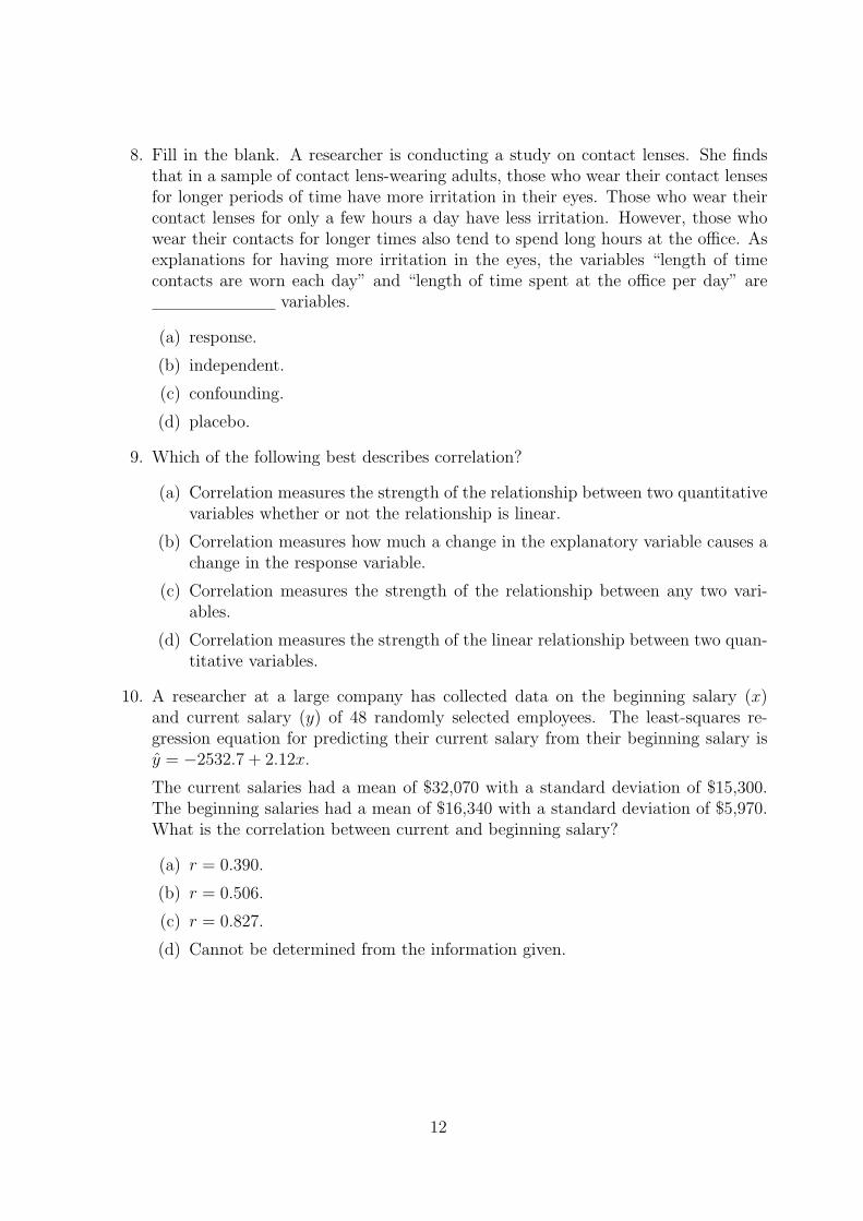
8. Fill in the blank. A researcher is conducting a study on contact lenses. She findsthat in a sample of contact lens-wearing adults, those who wear their contact lensesfor longer periods of time have more irritation in their eyes. Those who wear theircontact lenses for only a few hours a day have less irritation. However, those whowear their contacts for longer times also tend to spend long hours at the office. Asexplanations for having more irritation in the eyes, the variables “length of timecontacts are worn each day” and “length of time spent at the office per day” are

variables.

(a) response.

(b) independent.

(c) confounding.

(d) placebo.

9. Which of the following best describes correlation?

(a) Correlation measures the strength of the relationship between two quantitativevariables whether or not the relationship is linear.

(b) Correlation measures how much a change in the explanatory variable causes achange in the response variable.

(c) Correlation measures the strength of the relationship between any two vari-ables.

(d) Correlation measures the strength of the linear relationship between two quan-titative variables.

10. A researcher at a large company has collected data on the beginning salary (x)and current salary (y) of 48 randomly selected employees. The least-squares re-gression equation for predicting their current salary from their beginning salary isy = −2532.7 + 2.12x.

The current salaries had a mean of $32,070 with a standard deviation of $15,300.The beginning salaries had a mean of $16,340 with a standard deviation of $5,970.What is the correlation between current and beginning salary?

(a) r = 0.390.

(b) r = 0.506.

(c) r = 0.827.

(d) Cannot be determined from the information given.

12

11. A large study was done to compare two treatments for recurring ear infections inyoung children. A total of 150 subjects were recruited for the study, with 50 subjectsassigned at random to treatment 1 and the remainder to treatment 2. As part ofthe study, various types of demographic information were gathered. The followingtable classifies the mother’s education level into one of four categories for each ofthe treatment groups.

Under the null hypothesis that the distribution of mother’s educational level is thesame for both treatment groups, the expected number of mothers who are collegegrads for treatment 2 is

(a) 10.00.

(b) 13.33.

(c) 20.00.

(d) 25.00.

12. A table has 4 rows and 5 columns. The degrees of freedom for a χ2 test are

(a) 9.

(b) 10.

(c) 12.

(d) 20.

13. We are interested in comparing the proportions of males and females who thinkearning a large salary is very important to them. I surveyed 200 of each gender andrecorded their answers to the question as “yes” or “no”. If I analyze the data withboth a z-test for two proportions and a χ2 test of no association, the p-value for thez-test

(a) Will be less than for the χ2 test.

(b) Will be the same as for the χ2 test.

(c) Will be more than for the χ2 test.

(d) It is meaningless to compare these numerical results as they measure two totallydifferent things.

13

14. A study was conducted to explore the relationship between a child’s birth orderand his or her chances of becoming a juvenile delinquent. The subjects included arandom sample of girls enrolled in public high schools in a large city. Each subjectfilled out a questionnaire that measured whether or not they had shown delinquentbehavior, and their birth order. The data are given in the table below.

The value of the χ2 statistic for this data set is 21.236. The P-value is

(a) less than 0.0005.

(b) between 0.0005 and 0.001.

(c) between 0.001 and 0.0025.

(d) between 0.0025 and 0.005.

15. In the table below we examine the relationship between final grade and the reportedhours per week each student said they studied for the course.

The size of this table is

(a) 7 × 5.

(b) 5 × 7.

(c) 4 × 6.

(d) 3 × 5.

14

16. I have computed an analysis of variance for 3 groups with 10 observations per group.The degrees of freedom for the F test are

(a) 3 and 30.

(b) 2 and 10.

(c) 2 and 9.

(d) 2 and 27.

17. I have computed an Analysis of Variance (ANOVA) F test and obtained a p-valueof 0.001. This means

(a) All the groups have the same mean.

(b) All the group means are different.

(c) Some of the group means differ from the others.

(d) The result is biased.

18. I have 3 groups for which I want to perform an ANOVA. They have standarddeviations s1 = 2.5, s2 = 3.4, s3 = 6.4 and the plots of the data indicate all samplesare approximately normal with no outliers. Is the ANOVA appropriate?

(a) Yes — because the data are approximately normal distributed.

(b) Yes — because there are no outliers.

(c) No.

(d) I do not have enough information to tell.

19. The heights (in inches) of adult males in the U.S. are believed to be normallydistributed with mean µ. The average height of a random sample of 25 Americanadult males is found to be x = 69.72 inches and the standard deviation of the 25heights is found to be s = 4.15. A 90% confidence interval for µ is

(a) 69.72± 1.06.

(b) 69.72± 1.09.

(c) 69.72± 1.37.

(d) 69.72± 1.42.

15

20. It has been claimed that women live longer than men; however, men tend to beolder than their wives. Ages of 16 deceased husbands and wives from Englandwere obtained via a simple random sample of death records. These data should beanalyzed with a

(a) Two-sample t-test.

(b) Paired samples t-test

(c) Two-sample z-test.

(d) χ2 test.

21. The mathematical expression 5! (read 5 factorial) numerically results in

(a) 1.

(b) 5.

(c) 24.

(d) 120.

22. The mathematical expression(

64

)(read 6 choose 4) numerically results in

(a) 1.5.

(b) 10.

(c) 15.

(d) 30.

23. The time for students to complete a standardized placement exam given to collegefreshman has a normal distribution with a mean of 45 minutes and a standarddeviation of 10 minutes. If students are given one hour to complete the exam, theproportion of students who will complete the exam is about

(a) 0.17.

(b) 0.40.

(c) 0.60.

(d) 0.93.

24. The scores on a university examination are normally distributed with a mean of 65and a standard deviation of 11. If the top 8% of students are given A’s, what is thelowest mark that a student can have and still be awarded an A?

(a) 49.5.

(b) 76.1.

(c) 80.5.

(d) 84.2.

16

25. In a particular game, a ball is randomly chosen from a box that contains 2 red balls,2 green ball, and 6 blue balls. If a red ball is selected you win $2, if a green ball isselected you win $4, and if a blue ball is selected you win nothing. Let X be theamount that you win. The expected value of X is

(a) $1.20.

(b) $1.50.

(c) $2.00.

(d) $3.00.

26. You decide to test a friend for ESP using a standard deck of 52 playing cards. Sucha deck contains 13 spades, 13 hearts, 13 diamonds, and 13 clubs. You shuffle thedeck, select a card at random, and ask your friend to tell you whether the card isa spade, heart, diamond, or club. After the guess you return the card to the deck,shuffle the cards, and repeat the above. You do this a total of 80 times. Let X bethe number of correct guesses by your friend in the 80 trials. The standard deviationof X is

(a) about 0.05.

(b) about 3.87.

(c) about 15.65.

(d) about 225.87.

27. Incomes in a certain town are strongly right skewed with mean $40,000 and standarddeviation $8,000. A random sample of 5 households is taken. What is the probabilitythe average of the sample is more than $42,000?

(a) 0.29.

(b) 0.40.

(c) 0.60.

(d) Cannot say.

17

Use the following to answer questions 28, 29, and 30:

In statistics, we usually refer to x1 as the first observation, x2 as the second obser-vation, etc., and xn as the final observation when we write down our observations inthe order they were obtained (where n represents the total number of observations).

Often, we prefer to work with data that are sorted from smallest to largest, e.g.,when calculating the median, we need the data to be sorted. Obviously, we cansimply reorder any given list of numbers. However, we often use the notation x(1)

to refer to the smallest observation, x(2) to refer to the 2nd smallest observation,etc., and x(n) to refer to the largest observation.

28. For x1 = 3, x2 = −7, x3 = −5, x4 = −2, x5 = 5, x6 = 7, and n = 6, the sum

n−1∑i=2

xi =

equals

(a) −30.

(b) −12.

(c) −9.

(d) 1.

29. For x1 = 3, x2 = −7, x3 = −5, x4 = −2, x5 = 5, x6 = 7, and n = 6, the sum

n−1∑i=2

x(i) =

equals

(a) −30.

(b) −12.

(c) −9.

(d) 1.

30. For x1 = 3, x2 = −7, x3 = −5, x4 = −2, x5 = 5, x6 = 7, and n = 6, the sum

n∑i=1

x(3) =

equals

(a) −30.

(b) −12.

(c) −9.

(d) 1.

18

TABLES

You can remove the following 2 sheets of tables from the exam. No need toturn in these tables once they have been removed.

T-2•

Tables

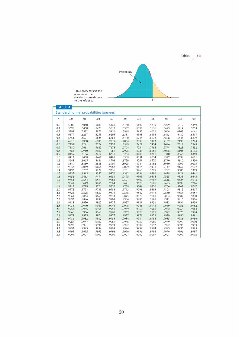
Table entry for z isthe area under thestandard normal curveto the left of z.

Probability

z

TABLE A

Standard normal probabilities

z .00 .01 .02 .03 .04 .05 .06 .07 .08 .09

−3.4 .0003 .0003 .0003 .0003 .0003 .0003 .0003 .0003 .0003 .0002−3.3 .0005 .0005 .0005 .0004 .0004 .0004 .0004 .0004 .0004 .0003−3.2 .0007 .0007 .0006 .0006 .0006 .0006 .0006 .0005 .0005 .0005−3.1 .0010 .0009 .0009 .0009 .0008 .0008 .0008 .0008 .0007 .0007−3.0 .0013 .0013 .0013 .0012 .0012 .0011 .0011 .0011 .0010 .0010−2.9 .0019 .0018 .0018 .0017 .0016 .0016 .0015 .0015 .0014 .0014−2.8 .0026 .0025 .0024 .0023 .0023 .0022 .0021 .0021 .0020 .0019−2.7 .0035 .0034 .0033 .0032 .0031 .0030 .0029 .0028 .0027 .0026−2.6 .0047 .0045 .0044 .0043 .0041 .0040 .0039 .0038 .0037 .0036−2.5 .0062 .0060 .0059 .0057 .0055 .0054 .0052 .0051 .0049 .0048−2.4 .0082 .0080 .0078 .0075 .0073 .0071 .0069 .0068 .0066 .0064−2.3 .0107 .0104 .0102 .0099 .0096 .0094 .0091 .0089 .0087 .0084−2.2 .0139 .0136 .0132 .0129 .0125 .0122 .0119 .0116 .0113 .0110−2.1 .0179 .0174 .0170 .0166 .0162 .0158 .0154 .0150 .0146 .0143−2.0 .0228 .0222 .0217 .0212 .0207 .0202 .0197 .0192 .0188 .0183−1.9 .0287 .0281 .0274 .0268 .0262 .0256 .0250 .0244 .0239 .0233−1.8 .0359 .0351 .0344 .0336 .0329 .0322 .0314 .0307 .0301 .0294−1.7 .0446 .0436 .0427 .0418 .0409 .0401 .0392 .0384 .0375 .0367−1.6 .0548 .0537 .0526 .0516 .0505 .0495 .0485 .0475 .0465 .0455−1.5 .0668 .0655 .0643 .0630 .0618 .0606 .0594 .0582 .0571 .0559−1.4 .0808 .0793 .0778 .0764 .0749 .0735 .0721 .0708 .0694 .0681−1.3 .0968 .0951 .0934 .0918 .0901 .0885 .0869 .0853 .0838 .0823−1.2 .1151 .1131 .1112 .1093 .1075 .1056 .1038 .1020 .1003 .0985−1.1 .1357 .1335 .1314 .1292 .1271 .1251 .1230 .1210 .1190 .1170−1.0 .1587 .1562 .1539 .1515 .1492 .1469 .1446 .1423 .1401 .1379−0.9 .1841 .1814 .1788 .1762 .1736 .1711 .1685 .1660 .1635 .1611−0.8 .2119 .2090 .2061 .2033 .2005 .1977 .1949 .1922 .1894 .1867−0.7 .2420 .2389 .2358 .2327 .2296 .2266 .2236 .2206 .2177 .2148−0.6 .2743 .2709 .2676 .2643 .2611 .2578 .2546 .2514 .2483 .2451−0.5 .3085 .3050 .3015 .2981 .2946 .2912 .2877 .2843 .2810 .2776−0.4 .3446 .3409 .3372 .3336 .3300 .3264 .3228 .3192 .3156 .3121−0.3 .3821 .3783 .3745 .3707 .3669 .3632 .3594 .3557 .3520 .3483−0.2 .4207 .4168 .4129 .4090 .4052 .4013 .3974 .3936 .3897 .3859−0.1 .4602 .4562 .4522 .4483 .4443 .4404 .4364 .4325 .4286 .4247

0.0 .5000 .4960 .4920 .4880 .4840 .4801 .4761 .4721 .4681 .4641

Integre Technical Publishing Co., Inc. Moore/McCabe November 16, 2007 1:29 p.m. moore page T-2

19

Tables•

T-3

Table entry for z is thearea under thestandard normal curveto the left of z.

Probability

z

TABLE A

Standard normal probabilities (continued)

z .00 .01 .02 .03 .04 .05 .06 .07 .08 .09

0.0 .5000 .5040 .5080 .5120 .5160 .5199 .5239 .5279 .5319 .53590.1 .5398 .5438 .5478 .5517 .5557 .5596 .5636 .5675 .5714 .57530.2 .5793 .5832 .5871 .5910 .5948 .5987 .6026 .6064 .6103 .61410.3 .6179 .6217 .6255 .6293 .6331 .6368 .6406 .6443 .6480 .65170.4 .6554 .6591 .6628 .6664 .6700 .6736 .6772 .6808 .6844 .68790.5 .6915 .6950 .6985 .7019 .7054 .7088 .7123 .7157 .7190 .72240.6 .7257 .7291 .7324 .7357 .7389 .7422 .7454 .7486 .7517 .75490.7 .7580 .7611 .7642 .7673 .7704 .7734 .7764 .7794 .7823 .78520.8 .7881 .7910 .7939 .7967 .7995 .8023 .8051 .8078 .8106 .81330.9 .8159 .8186 .8212 .8238 .8264 .8289 .8315 .8340 .8365 .83891.0 .8413 .8438 .8461 .8485 .8508 .8531 .8554 .8577 .8599 .86211.1 .8643 .8665 .8686 .8708 .8729 .8749 .8770 .8790 .8810 .88301.2 .8849 .8869 .8888 .8907 .8925 .8944 .8962 .8980 .8997 .90151.3 .9032 .9049 .9066 .9082 .9099 .9115 .9131 .9147 .9162 .91771.4 .9192 .9207 .9222 .9236 .9251 .9265 .9279 .9292 .9306 .93191.5 .9332 .9345 .9357 .9370 .9382 .9394 .9406 .9418 .9429 .94411.6 .9452 .9463 .9474 .9484 .9495 .9505 .9515 .9525 .9535 .95451.7 .9554 .9564 .9573 .9582 .9591 .9599 .9608 .9616 .9625 .96331.8 .9641 .9649 .9656 .9664 .9671 .9678 .9686 .9693 .9699 .97061.9 .9713 .9719 .9726 .9732 .9738 .9744 .9750 .9756 .9761 .97672.0 .9772 .9778 .9783 .9788 .9793 .9798 .9803 .9808 .9812 .98172.1 .9821 .9826 .9830 .9834 .9838 .9842 .9846 .9850 .9854 .98572.2 .9861 .9864 .9868 .9871 .9875 .9878 .9881 .9884 .9887 .98902.3 .9893 .9896 .9898 .9901 .9904 .9906 .9909 .9911 .9913 .99162.4 .9918 .9920 .9922 .9925 .9927 .9929 .9931 .9932 .9934 .99362.5 .9938 .9940 .9941 .9943 .9945 .9946 .9948 .9949 .9951 .99522.6 .9953 .9955 .9956 .9957 .9959 .9960 .9961 .9962 .9963 .99642.7 .9965 .9966 .9967 .9968 .9969 .9970 .9971 .9972 .9973 .99742.8 .9974 .9975 .9976 .9977 .9977 .9978 .9979 .9979 .9980 .99812.9 .9981 .9982 .9982 .9983 .9984 .9984 .9985 .9985 .9986 .99863.0 .9987 .9987 .9987 .9988 .9988 .9989 .9989 .9989 .9990 .99903.1 .9990 .9991 .9991 .9991 .9992 .9992 .9992 .9992 .9993 .99933.2 .9993 .9993 .9994 .9994 .9994 .9994 .9994 .9995 .9995 .99953.3 .9995 .9995 .9995 .9996 .9996 .9996 .9996 .9996 .9996 .99973.4 .9997 .9997 .9997 .9997 .9997 .9997 .9997 .9997 .9997 .9998

Integre Technical Publishing Co., Inc. Moore/McCabe November 16, 2007 1:29 p.m. moore page T-3

20

Tables•

T-11

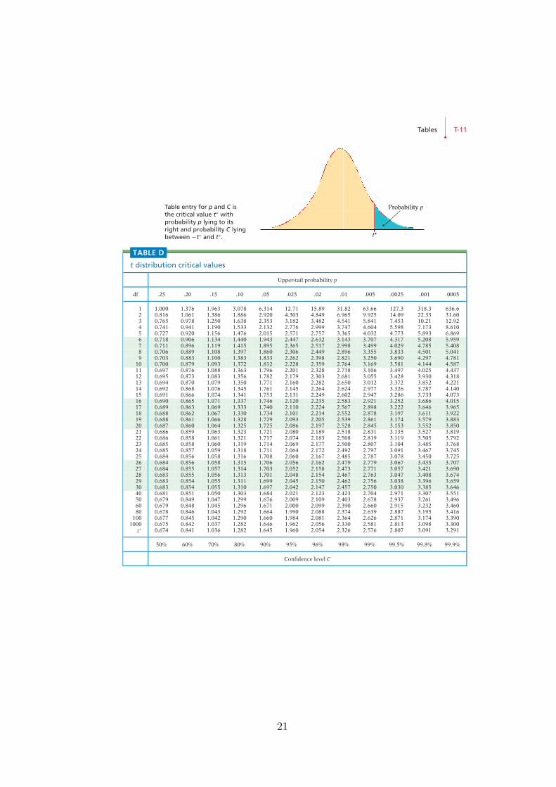
Table entry for p and C isthe critical value t∗ withprobability p lying to itsright and probability C lyingbetween −t∗ and t∗.

Probability p

t*

TABLE D

t distribution critical values

Upper-tail probability p

df .25 .20 .15 .10 .05 .025 .02 .01 .005 .0025 .001 .0005

1 1.000 1.376 1.963 3.078 6.314 12.71 15.89 31.82 63.66 127.3 318.3 636.62 0.816 1.061 1.386 1.886 2.920 4.303 4.849 6.965 9.925 14.09 22.33 31.603 0.765 0.978 1.250 1.638 2.353 3.182 3.482 4.541 5.841 7.453 10.21 12.924 0.741 0.941 1.190 1.533 2.132 2.776 2.999 3.747 4.604 5.598 7.173 8.6105 0.727 0.920 1.156 1.476 2.015 2.571 2.757 3.365 4.032 4.773 5.893 6.8696 0.718 0.906 1.134 1.440 1.943 2.447 2.612 3.143 3.707 4.317 5.208 5.9597 0.711 0.896 1.119 1.415 1.895 2.365 2.517 2.998 3.499 4.029 4.785 5.4088 0.706 0.889 1.108 1.397 1.860 2.306 2.449 2.896 3.355 3.833 4.501 5.0419 0.703 0.883 1.100 1.383 1.833 2.262 2.398 2.821 3.250 3.690 4.297 4.781

10 0.700 0.879 1.093 1.372 1.812 2.228 2.359 2.764 3.169 3.581 4.144 4.58711 0.697 0.876 1.088 1.363 1.796 2.201 2.328 2.718 3.106 3.497 4.025 4.43712 0.695 0.873 1.083 1.356 1.782 2.179 2.303 2.681 3.055 3.428 3.930 4.31813 0.694 0.870 1.079 1.350 1.771 2.160 2.282 2.650 3.012 3.372 3.852 4.22114 0.692 0.868 1.076 1.345 1.761 2.145 2.264 2.624 2.977 3.326 3.787 4.14015 0.691 0.866 1.074 1.341 1.753 2.131 2.249 2.602 2.947 3.286 3.733 4.07316 0.690 0.865 1.071 1.337 1.746 2.120 2.235 2.583 2.921 3.252 3.686 4.01517 0.689 0.863 1.069 1.333 1.740 2.110 2.224 2.567 2.898 3.222 3.646 3.96518 0.688 0.862 1.067 1.330 1.734 2.101 2.214 2.552 2.878 3.197 3.611 3.92219 0.688 0.861 1.066 1.328 1.729 2.093 2.205 2.539 2.861 3.174 3.579 3.88320 0.687 0.860 1.064 1.325 1.725 2.086 2.197 2.528 2.845 3.153 3.552 3.85021 0.686 0.859 1.063 1.323 1.721 2.080 2.189 2.518 2.831 3.135 3.527 3.81922 0.686 0.858 1.061 1.321 1.717 2.074 2.183 2.508 2.819 3.119 3.505 3.79223 0.685 0.858 1.060 1.319 1.714 2.069 2.177 2.500 2.807 3.104 3.485 3.76824 0.685 0.857 1.059 1.318 1.711 2.064 2.172 2.492 2.797 3.091 3.467 3.74525 0.684 0.856 1.058 1.316 1.708 2.060 2.167 2.485 2.787 3.078 3.450 3.72526 0.684 0.856 1.058 1.315 1.706 2.056 2.162 2.479 2.779 3.067 3.435 3.70727 0.684 0.855 1.057 1.314 1.703 2.052 2.158 2.473 2.771 3.057 3.421 3.69028 0.683 0.855 1.056 1.313 1.701 2.048 2.154 2.467 2.763 3.047 3.408 3.67429 0.683 0.854 1.055 1.311 1.699 2.045 2.150 2.462 2.756 3.038 3.396 3.65930 0.683 0.854 1.055 1.310 1.697 2.042 2.147 2.457 2.750 3.030 3.385 3.64640 0.681 0.851 1.050 1.303 1.684 2.021 2.123 2.423 2.704 2.971 3.307 3.55150 0.679 0.849 1.047 1.299 1.676 2.009 2.109 2.403 2.678 2.937 3.261 3.49660 0.679 0.848 1.045 1.296 1.671 2.000 2.099 2.390 2.660 2.915 3.232 3.46080 0.678 0.846 1.043 1.292 1.664 1.990 2.088 2.374 2.639 2.887 3.195 3.416

100 0.677 0.845 1.042 1.290 1.660 1.984 2.081 2.364 2.626 2.871 3.174 3.3901000 0.675 0.842 1.037 1.282 1.646 1.962 2.056 2.330 2.581 2.813 3.098 3.300

z∗ 0.674 0.841 1.036 1.282 1.645 1.960 2.054 2.326 2.576 2.807 3.091 3.291

50% 60% 70% 80% 90% 95% 96% 98% 99% 99.5% 99.8% 99.9%

Confidence level C

Integre Technical Publishing Co., Inc. Moore/McCabe November 16, 2007 1:29 p.m. moore page T-11

21

T-20•

Tables

Table entry for p is thecritical value (χ2)∗ withprobability p lying to itsright.

Probability p

( 2)*χ

TABLE F

χ2 distribution critical values

Tail probability p

df .25 .20 .15 .10 .05 .025 .02 .01 .005 .0025 .001 .0005

1 1.32 1.64 2.07 2.71 3.84 5.02 5.41 6.63 7.88 9.14 10.83 12.122 2.77 3.22 3.79 4.61 5.99 7.38 7.82 9.21 10.60 11.98 13.82 15.203 4.11 4.64 5.32 6.25 7.81 9.35 9.84 11.34 12.84 14.32 16.27 17.734 5.39 5.99 6.74 7.78 9.49 11.14 11.67 13.28 14.86 16.42 18.47 20.005 6.63 7.29 8.12 9.24 11.07 12.83 13.39 15.09 16.75 18.39 20.51 22.116 7.84 8.56 9.45 10.64 12.59 14.45 15.03 16.81 18.55 20.25 22.46 24.107 9.04 9.80 10.75 12.02 14.07 16.01 16.62 18.48 20.28 22.04 24.32 26.028 10.22 11.03 12.03 13.36 15.51 17.53 18.17 20.09 21.95 23.77 26.12 27.879 11.39 12.24 13.29 14.68 16.92 19.02 19.68 21.67 23.59 25.46 27.88 29.67

10 12.55 13.44 14.53 15.99 18.31 20.48 21.16 23.21 25.19 27.11 29.59 31.4211 13.70 14.63 15.77 17.28 19.68 21.92 22.62 24.72 26.76 28.73 31.26 33.1412 14.85 15.81 16.99 18.55 21.03 23.34 24.05 26.22 28.30 30.32 32.91 34.8213 15.98 16.98 18.20 19.81 22.36 24.74 25.47 27.69 29.82 31.88 34.53 36.4814 17.12 18.15 19.41 21.06 23.68 26.12 26.87 29.14 31.32 33.43 36.12 38.1115 18.25 19.31 20.60 22.31 25.00 27.49 28.26 30.58 32.80 34.95 37.70 39.7216 19.37 20.47 21.79 23.54 26.30 28.85 29.63 32.00 34.27 36.46 39.25 41.3117 20.49 21.61 22.98 24.77 27.59 30.19 31.00 33.41 35.72 37.95 40.79 42.8818 21.60 22.76 24.16 25.99 28.87 31.53 32.35 34.81 37.16 39.42 42.31 44.4319 22.72 23.90 25.33 27.20 30.14 32.85 33.69 36.19 38.58 40.88 43.82 45.9720 23.83 25.04 26.50 28.41 31.41 34.17 35.02 37.57 40.00 42.34 45.31 47.5021 24.93 26.17 27.66 29.62 32.67 35.48 36.34 38.93 41.40 43.78 46.80 49.0122 26.04 27.30 28.82 30.81 33.92 36.78 37.66 40.29 42.80 45.20 48.27 50.5123 27.14 28.43 29.98 32.01 35.17 38.08 38.97 41.64 44.18 46.62 49.73 52.0024 28.24 29.55 31.13 33.20 36.42 39.36 40.27 42.98 45.56 48.03 51.18 53.4825 29.34 30.68 32.28 34.38 37.65 40.65 41.57 44.31 46.93 49.44 52.62 54.9526 30.43 31.79 33.43 35.56 38.89 41.92 42.86 45.64 48.29 50.83 54.05 56.4127 31.53 32.91 34.57 36.74 40.11 43.19 44.14 46.96 49.64 52.22 55.48 57.8628 32.62 34.03 35.71 37.92 41.34 44.46 45.42 48.28 50.99 53.59 56.89 59.3029 33.71 35.14 36.85 39.09 42.56 45.72 46.69 49.59 52.34 54.97 58.30 60.7330 34.80 36.25 37.99 40.26 43.77 46.98 47.96 50.89 53.67 56.33 59.70 62.1640 45.62 47.27 49.24 51.81 55.76 59.34 60.44 63.69 66.77 69.70 73.40 76.0950 56.33 58.16 60.35 63.17 67.50 71.42 72.61 76.15 79.49 82.66 86.66 89.5660 66.98 68.97 71.34 74.40 79.08 83.30 84.58 88.38 91.95 95.34 99.61 102.780 88.13 90.41 93.11 96.58 101.9 106.6 108.1 112.3 116.3 120.1 124.8 128.3

100 109.1 111.7 114.7 118.5 124.3 129.6 131.1 135.8 140.2 144.3 149.4 153.2

Integre Technical Publishing Co., Inc. Moore/McCabe November 16, 2007 1:29 p.m. moore page T-20

22