Statistical/Evolutionary Models of Power-laws in Plasmas
54
Statistical/Evolutionary Models of Power-laws in Plasmas Ilan Roth Space Sciences, UC Berkeley Halkidiki GREECE June 2009 Modern Challenges in Nonlinear Plasma Physics
Transcript of Statistical/Evolutionary Models of Power-laws in Plasmas
Statistical/Evolutionary Models of Power-laws in Plasmas
Ilan Roth
Space Sciences, UC Berkeley
Halkidiki
GREECE
June 2009
Modern Challenges in Nonlinear Plasma Physics

Heavy Tails
- Statistics of Energization Processes
- Anomalous Transport/Diffusion
- Entropy of Super-diffusive Processes
BASICS: Ergodic, weakly interacting system
converges into Boltzmann-Gibbs statistics/function
THEREFORE: particles that interact stochastically with electromagnetic fields and perform Brownian motion in phase space, characterized by short-range deviation and short term microscopic memory will approach asymptotically a Gaussian.
Why is there an ubiquity of (broken) power laws?
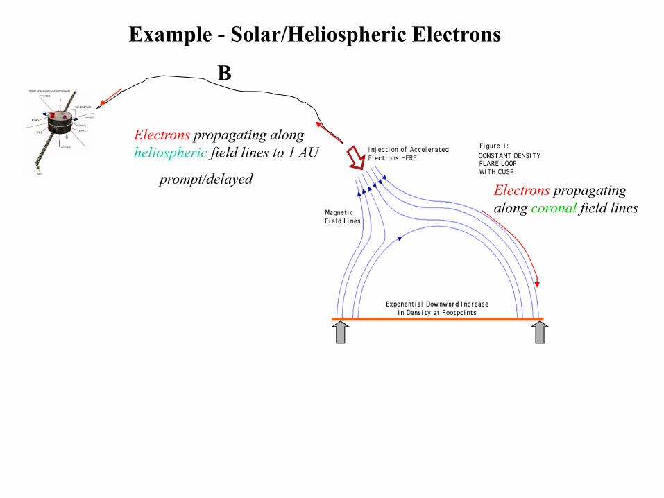
Example - Solar/Heliospheric Electrons
Electrons propagating along heliospheric field lines to 1 AU
prompt/delayedElectrons propagating along coronal field lines
B
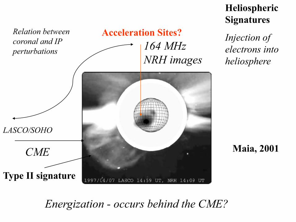
164 MHz NRH images
LASCO/SOHO
Relation between coronal and IP perturbations
Heliospheric Signatures
Injection of electrons into heliosphere
CME Maia, 2001
Energization - occurs behind the CME?
Acceleration Sites?
Type II signature

Post-flare, post-CME: Gradual electrons
Distinct delay between Type III and energetic electron injections
Impulsive
Gradual

gradual
impulsive
Electron Spectra

Yellow – flare site Black arrow – CME direction
Red – closed (stretched) magnetic field lines
Blue - open, in ecliptic plane
green – open, non-ecliptic
Wang, 2006
Post CME reconstruction

Yellow – flare site Black arrow – CME direction
Red – closed (stretched) magnetic field lines
Blue - open, in ecliptic plane green – open, non-ecliptic
CME

Characteristics of electron trajectory in the presence of (oblique) whistler waves

Statistics of Energization Processes- Anomalous Transport/Diffusion
- Entropy of Super-diffusive Processes

Statistical Analysis – Particle Distribution
Energization is determined by an increment of an independent, identically distributed (iid) random variable (in the language of statistical mathematics), with an assigned probability distribution.

Central Limit Theorem (CLT):
Sum of random variables with a finite variance will converge (weakly) to a normal or Gaussian distribution.
No Heavy Tail. Stable Distribution: addition of a large number of random variables preserves the shape of the distribution (infinitely divisible). Normal Distribution is an example of a Stable Distribution (“attractor distribution”).
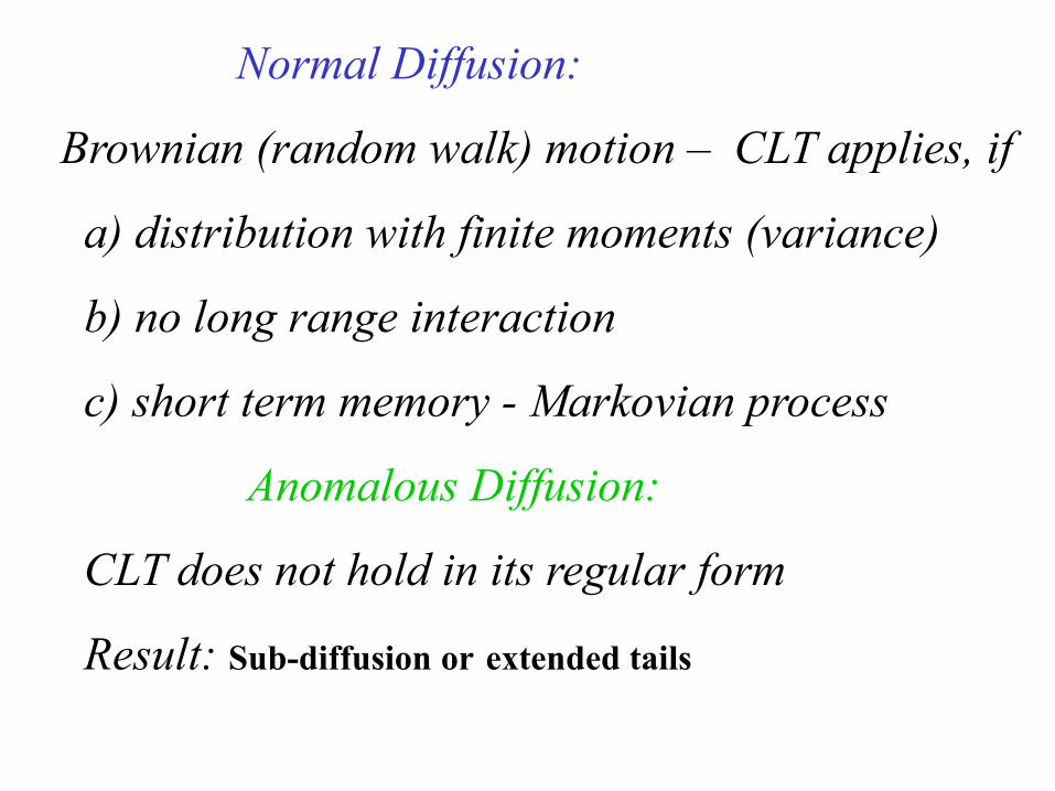
Normal Diffusion:
Brownian (random walk) motion – CLT applies, if
a) distribution with finite moments (variance)
b) no long range interaction
c) short term memory - Markovian process
Anomalous Diffusion:
CLT does not hold in its regular form
Result: Sub-diffusion or extended tails

yprobabilitnormalthepreservesnConvolutio
cdcNYcbadbac
ondistributiinYdcXbXaXdc
bbNbXaaNaX
vrddistributeyidenticallnottindependenXX
dxxxXPNXx
)(
])(,[~;)(,
)(:,
])(,[~],)(,[~
,.)(,,
]2/)(exp[2
1)();,(~
2222
21
22
21
21
22
2
2
σμμ
σμσμ
σμπσ
σμ
+−+=+=
=+=+∃
−−
−−=≤ ∫∞−
This (stable) Distribution is not unique
Normal Distribution
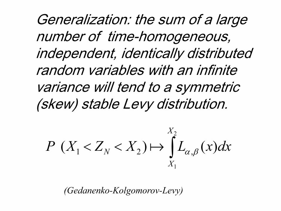
Generalization: the sum of a large number of time-homogeneous, independent, identically distributed random variables with an infinite variance will tend to a symmetric (skew) stable Levy distribution.
∫<<2
1
)()( ,21
X
XN dxxLXZXP βα
(Gedanenko-Kolgomorov-Levy)

Lévy (α stable) Probability Distribution The stable distribution functions are completely
defined by their Characteristic Function
(Fourier Transform of a single event probability)
– Lévy exponent, c – scale, β - skewness
( Gaussian : α = 2; Lorentzian /Cauchy: α = 1)
α=2 – “phase transition”Normal law attracts all distributions with α > 2
])sgn()2/tan(1exp[)( )(^
λπαβλλ αα icl −−=
20 ≤≤ α

Probability density function of stable Levy distributions
α-exponent; μ-shift; c=σ-width/scale; β-skewness
As α decreases, longer tail and narrower core δ function.
Cauchy
Gaussian
Holtsmark


Cumulative Distribution Function
Gaussian
Cauchy
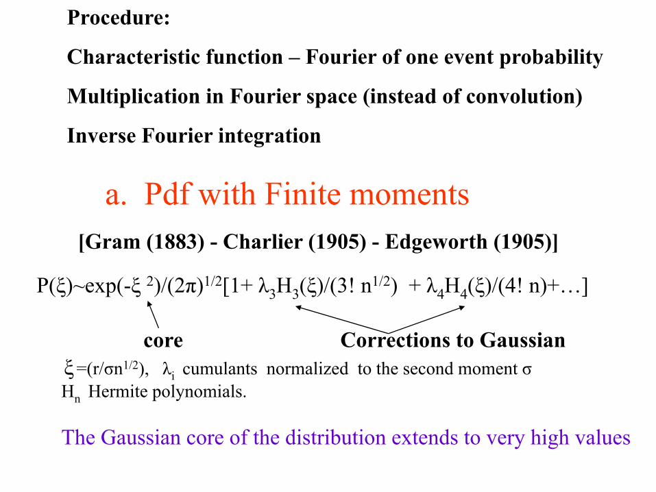
a. Pdf with Finite moments
P(ξ)~exp(-ξ 2)/(2π)1/2[1+ λ3H3(ξ)/(3! n1/2) + λ4H4(ξ)/(4! n)+…]
[Gram (1883) - Charlier (1905) - Edgeworth (1905)]
ξ=(r/σn1/2), λi cumulants normalized to the second moment σHn Hermite polynomials.
The Gaussian core of the distribution extends to very high values
Corrections to Gaussian
Procedure:
Characteristic function – Fourier of one event probability
Multiplication in Fourier space (instead of convolution)
Inverse Fourier integration
core

b. Leptokurtotic probability function (diverging high (>2) moments)
]2
sin2
)[cos2
exp()(:
)1(/2)(:
^
4
2/1
ηηηη
π
+−
=
+=
pFunctionsticCharacteri
rrpyprobabiliteventOne
πη
ηη
ηη
2)(
)](exp[log()(
)]([log
^^
^ deerP
pp
pnirn ∫=
=

dyeerDIntegralDawsonDGaussianr
nDOrD
nrr
dirrrn
r
dn
aeer
ryr
G
Gn
G
irn
∫
∫
∫
−
−
=−−Φ
++′′′−+ΦΦ
−−−∂∂
+Φ
++=Φ
0
)4(
2/12/1
223
3
2/1
32/
22
2
)(:;)(
...][)2
(62
)1()(~)(
})(exp[)2/{exp()62
1)(~
~2
...]1[)(
π
ηηπ
πηηηη
Cumulant expansion - log p(η) around η =0
....48/1123/2/)(log 432^
+++−= ηηηηp

]2
!)!12(43
211[
22~)( 2342 mmm x
mxxx
xD −+++ Σ∞
=
The edge of the central core ~ (log n)1/2
Due to limited interaction time, the observed distribution converges extremely slowly to a Gaussian and exhibits heavy tails.
]288/12/[)62
1)(~)(
3/1~)(
642/1
4
nn
xasxxD
Gn−− ++ΦΦ
∞>−−′′′
ξξπ
ξξ

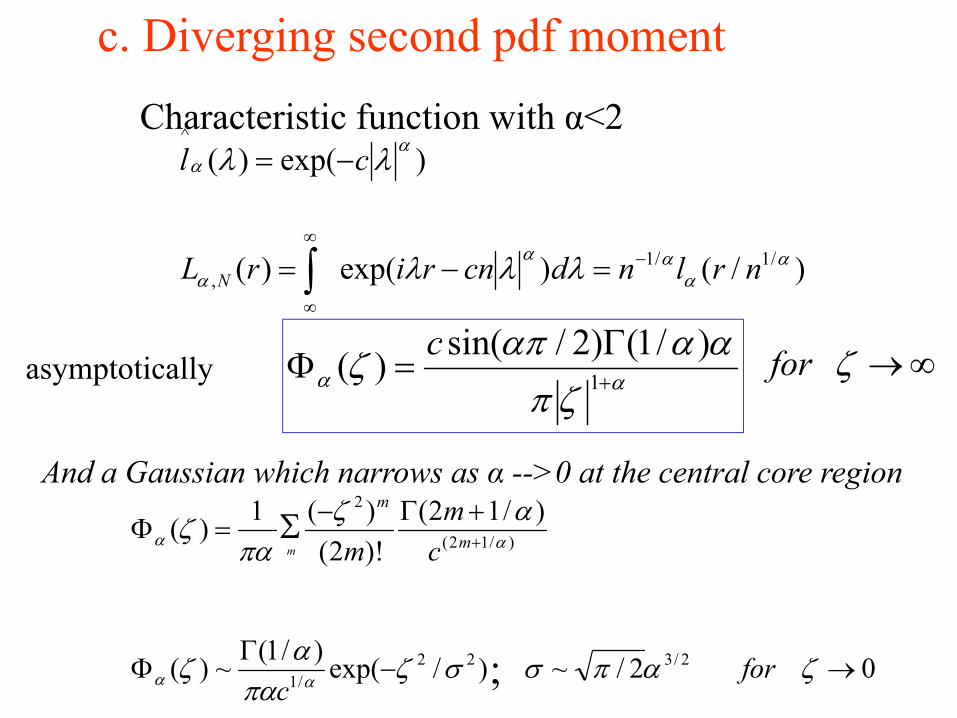
c. Diverging second pdf momentCharacteristic function with α<2
ααζπ
αααπζ +
Γ=Φ 1
)/1()2/sin()( c ∞→ζfor
02/~)/exp()/1(~)(
)/12()!2()(1)(
2/322/1
)/12(
2
; →−Γ
Φ
+Γ−=Φ +Σ
ζαπσσζπα
αζ
αζπα
ζ
αα
αα
forc
cm
m m
m
m
And a Gaussian which narrows as α -->0 at the central core region
)/()exp()(
)exp()(
/1/1,
^
αα
ααα
αα
λλλ
λλ
nrlndcnrirL
cl
N−
∞
∞
=−=
−=
∫
asymptotically


Gaussian
T-student
Truncated Cauchy
- Statistics of Energization Processes
Anomalous Transport/Diffusion- Entropy of Super-diffusive Processes

Random walk: continuum description FP
jumpsisotropicrrr
tPtPttP
ii
iii
;
);(21)(
21)(
1
11
Δ±=
+=Δ+
±
−+
Central limit theorem
),(),()(),(2
2
2
22
,0lim trP
rKtrP
rdtdr
ttrP
odtdr ∂∂
≡∂∂
=∂
∂
→→
<r2> ~ tα ; α=1
)4/exp()4(),( 22/1 KtrKttrP −= −π
Continuum limit
Local in space and time
Phase space
Green propagator

Continuous time Random walk
Length of jump, waiting time
χ(r, t) = λ(r)τ(t)
Decoupled temporal/spatial memory
Probabilities
λ(r)dr phase space jump
τ(t)dt waiting time between jumps
Pj(t+dt)=∑n=1 [Aj,nPj-n(t)+ Bj,nPj+n (t)]
Non-locality in phase space
Generalization

),(
),(),(
tx
txvtxk
Ω
−=ω
ν
ν=n Waiting time
jump

Fourier-Laplace(Montroll-Weiss) ),(1
)(1),( 0
ukP
uuukP
χτ
−−
=
Probability P(r,t) - phase space position r at time t probability ζ(r,t’) of arrival at r at an earlier time t’ and staying there without a jump:“survival” probability φ(t)=1-∫dt τ(t);
P(r,t) = ∫dt’ ζ(r,t’) φ(t-t’)
Master equation
ζ (r,t)= ∫dr’ ∫dt’ ζ(r’,t’) χ(r-r’,t-t’) + Po(r) δ(t)
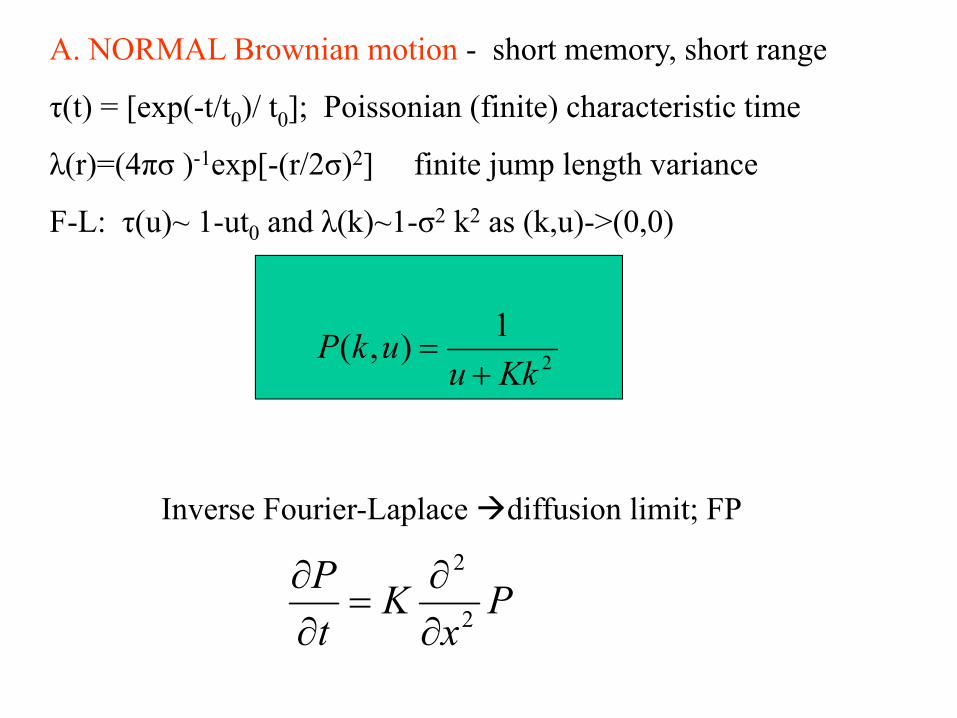
A. NORMAL Brownian motion - short memory, short range
τ(t) = [exp(-t/t0)/ t0]; Poissonian (finite) characteristic time
λ(r)=(4πσ )-1exp[-(r/2σ)2] finite jump length variance
F-L: τ(u)~ 1-ut0 and λ(k)~1-σ2 k2 as (k,u)->(0,0)
Inverse Fourier-Laplace diffusion limit; FP
2
1),(Kku
ukP+
=
Px
KtP
2
2
∂∂
=∂∂
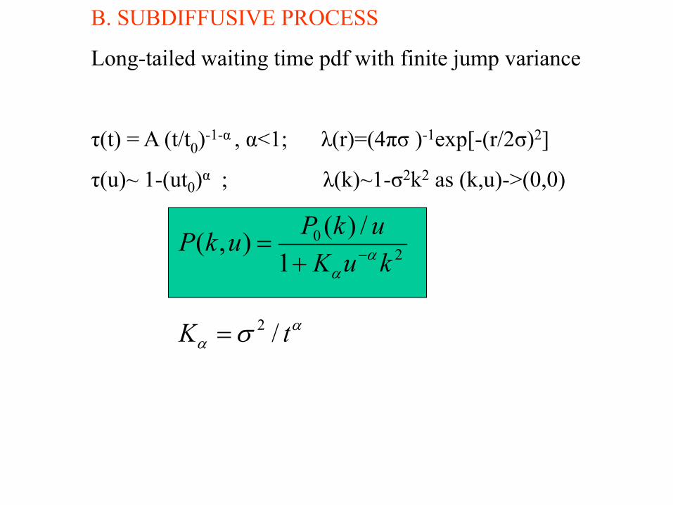
B. SUBDIFFUSIVE PROCESS
Long-tailed waiting time pdf with finite jump variance
τ(t) = A (t/t0)-1-α , α<1; λ(r)=(4πσ )-1exp[-(r/2σ)2]
τ(u)~ 1-(ut0)α ; λ(k)~1-σ2k2 as (k,u)->(0,0)
αα
αα
σ tK
kuKukPukP
/
1/)(),(
2
20
=
+= −
),(),(2
2
trPr
KDt
trPt ∂
∂=
∂∂ −
αα1
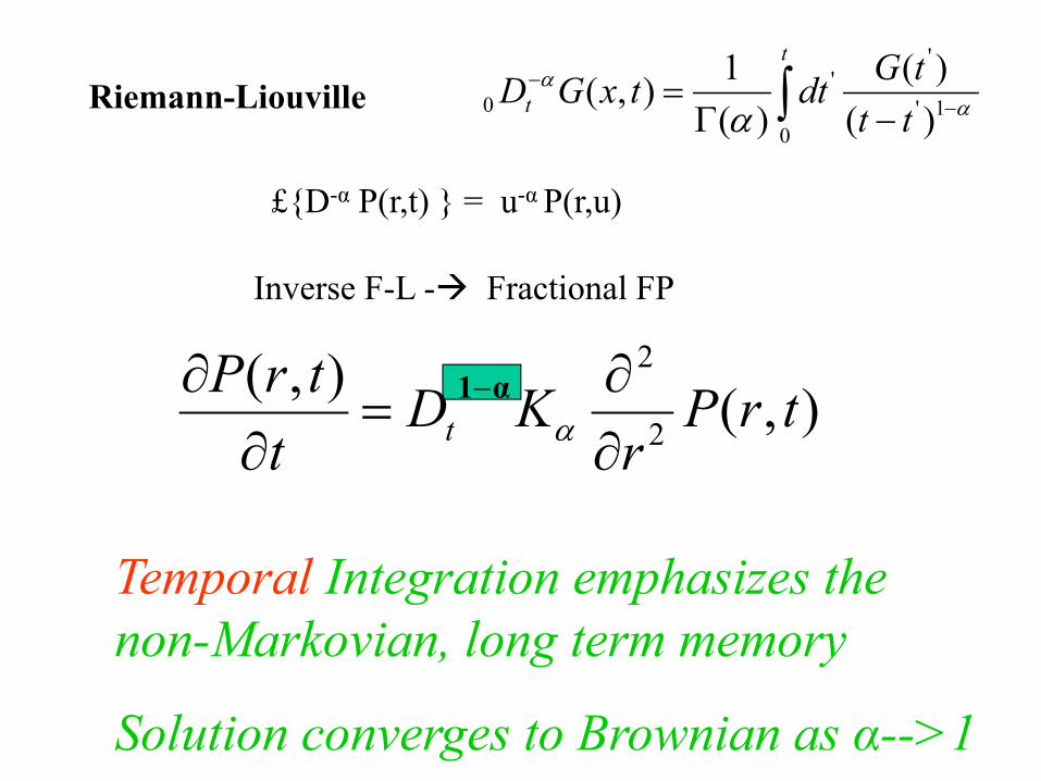
Temporal Integration emphasizes the non-Markovian, long term memory
Solution converges to Brownian as α-->1
£{D-α P(r,t) } = u-α P(r,u)
Inverse F-L - Fractional FP
∫ −−
−Γ=
t
t tttGdttxGD
01'
''
0 )()(
)(1),( α
α
αRiemann-Liouville
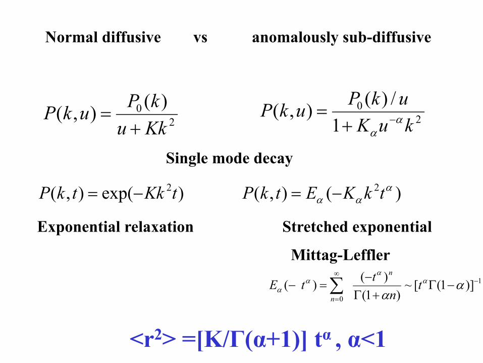
Normal diffusive vs anomalously sub-diffusive
20 )(),(KkukPukP
+= 2
0
1/)(),(
kuKukPukP α
α−+
=
)(),()exp(),( 22 ααα tkKEtkPtKktkP −=−=
Exponential relaxation Stretched exponential
Single mode decay
1
0)]1([~
)1()()( −
∞
=
−Γ+Γ
−=− ∑ α
αα
αα
α tn
ttEn
n
Mittag-Leffler
<r2> =[K/Γ(α+1)] tα , α<1

C. SUPERDIFFUSIVE PROCESS
Short memory waiting time - long jumps variance
Markovian time pdf Levy diverging jumps: μ<2
0
0
/
;)(),(
tK
kKukPukP
μμ
μμ
σ=
+=
μμμμ σσλτ k-1~)kexp(- (k) ;ut -1~ (u) 0 =

),(),( trPDKt
trPrμμ
∞−=∂
∂
),1()}({)}({:
)()(
)(1)()( )(1'
'')(
nnzGkzGDFourier
zzzGdz
dzd
nzGDzGD
z
z
nn
nnn
zz
−∈−=
−−Γ==
∞−
∞−−−
−−∞−∞− ∫
μ
μ
μμ
μμμ
FF
Spatial Integration emphasizes the probability for a long range interaction
Solution converges to Brownian as μ-->2
Riess/Weyl fractional operator

Gauss walk Levy flight

Normal diffusive vs anomalously super-diffusive
20 )(),(KkukPukP
+= μμkKu
kPukP+
=)(),( 0
)exp(),()exp(),( 2 tkKtkPtKktkP μμ−=−=
Exponential relaxation Extended tail
Symmetric Levy
Single mode decay
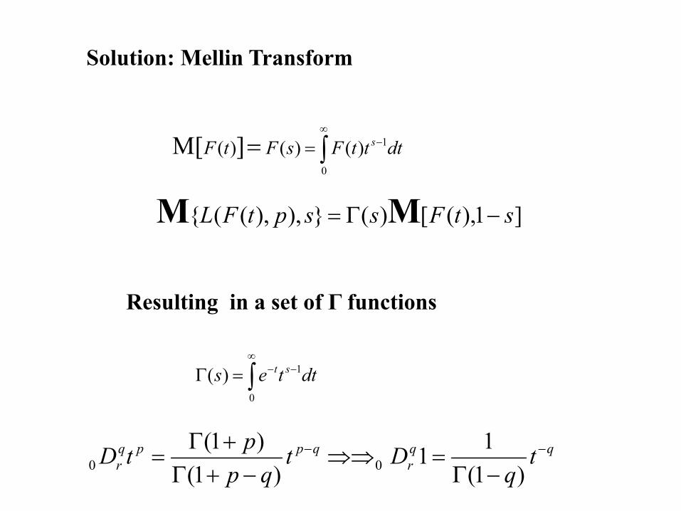
Solution: Mellin Transform
∫∞
−==0
1)()()( ]Μ[ dtttFsFtF s
∫∞
−−=Γ0
1)( dttes st
Resulting in a set of Γ functions
qqr
qppqr t
qDt
qpptD −−
−Γ=⇒⇒
−+Γ+Γ
=)1(
11)1(
)1(00
]1),([)(}),),(({ stFssptFL −Γ= MM

Gamma function – holomorphic with simple poles at all the non-positive integers; the residue at -n is (-1)n/n!

dszsasb
sasb
izHzH s
p
niii
q
miii
n
iii
m
iii
ab
mnpq
∏∏
∏∏∫
+=+=
==
−Γ+−Γ
−−Γ−Γ==
11
11
C
),(),(
)()1(
)1()(
21];[)(
αβ
αβ
παβ
Alternating signs – slow convergence
Series expansion with residue (-1)/l! at the poles bk-βks=-l, l=0,...
k
k lb
k
l
p
ni k
kii
q
mi k
kii
n
i k
kii
m
ki k
kii
l
m
k
ab
mnpq bl
zlbalbb
lbalbbzH
βαβ
βα
ββ
βα
ββ
)(
11
1,1
01
),(),( !
)1(
])([])(1[
])(1[])([];[
+
+=+=
=≠=∞
==
−+
−Γ+
+−Γ
++−Γ
+−Γ
=
∏∏
∏∏∑∑
αj,βj >0; aj,bj –complex; roots of (a, α)/ (b,β ) left/right of C
Fox (H) : generalized Mellin-Barnes (Meijer G) Functions

])/([)(),(/1/1 μ
μμ KtrLKttrP −=
s
Css
ssds
rH
rtrP ξ
μ
μμ
ξμ
μ
)1()2
(
)()1(1]|[1),( )2/1,1)(/1,1(
)2/1,1)(1,1(1122
−ΓΓ
Γ−Γ== ∫
Roots at s/μ=-m; ∑∞
=+
−−−ΓΓ
=0
1~!)1(
)2/()(1),(
m
mm
rKt
mmm
rtrP μ
μξμμ
μ
Explicit solution of the FFPE
μμξ /1)( tKr
=
poles
Slow convergence

General: Long waiting times and large jumps
),(),( 1 trPr
KDt
trPt μ
μμα
α
∂∂
=∂
∂ −
μα /2 tr >=<

- Statistics of Energization Processes
- Anomalous Transport/Diffusion
Entropy of Super-diffusive processes

*Thermodynamic properties - from microscopic states
*System in contact with a large reservoir
*Short temporal/spatial interaction – random jumps p(r)
Boltzmann-Gibbs-Shannon entropy-extensive ~system size
∫−== drrprpSSBG )(ln)(1
Constrains:
Variational Optimization; β-Lagrange multiplier
∞<=>=<= ∫∫ 222 )(;1)( σdrrprrdrrp
)2/(1;)exp()(
)exp()( 212
1
2
1 2 σββββ
β==
−=
−= −
−
∫T
dre
rZ
rrpr
Gaussian – attractor in distribution space

Long range interaction makes the entropy non-extensive
formation of tails in the distribution.
q-statistics/entropy (Tsallis):
Optimization of Sq with q-expectation constraint
and β as Lagrange multiplier leads to heavy tail distributions
1)1/(])(1[ 1 →=→∫ −−= qasSSqdrrqpqS BG
)exp(/])1(1[)( 2)1/(12 rZrqrp qq
q βπβ
β −→−−= −
q 1
drrprr q)]([22 ∫>=<
∫ −
−=
−==⇒⇒−+= −
)(exp)(exp
)()(exp
)(])1(1[2
22)1/(1
rdrr
Zr
rprqeq
q
q
qrq β
βββ

1<q<3 - Student t distribution 2/)1(2
)1(]2/[]2/)1[()( +−+
Γ+Γ
= k
kr
kkkrfπ
kkq
++
=13
qxpdxx )(2∫
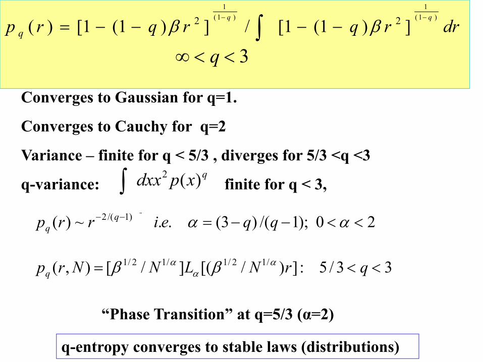
Converges to Gaussian for q=1.
Converges to Cauchy for q=2
Variance – finite for q < 5/3 , diverges for 5/3 <q <3
q-variance: finite for q < 3,
drrqrqrpqq
q)1(
1)1(
1
])1(1[/])1(1[)( 22 −−
−−−−= ∫ ββ
3<<∞ q
33/5:])/[(]/[),(
20);1/()3(..~)(
/12/1/12/1
)1/(2
<<=
<<−−=−−
qrNLNNrp
qqeirrp
q
αα
α ββ
αα
q-entropy converges to stable laws (distributions)
“Phase Transition” at q=5/3 (α=2)

Comparison with the data allows to assess a) the validity of the single event probability
density function
b) the relative importance of the different expansion terms – power law transition
c) the “duration” of the interaction
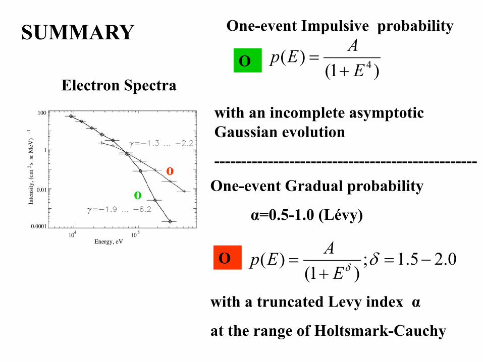
One-event Gradual probability
α=0.5-1.0 (Lévy)
with a truncated Levy index α
at the range of Holtsmark-Cauchy
One-event Impulsive probability
with an incomplete asymptotic Gaussian evolution
-------------------------------------------------
Electron Spectra)1(
)( 4EAEp+
=
0.25.1;)1(
)( −=+
= δδEAEp
O
O
oo
SUMMARY
ΕΠΙΛΟΓΟΣDistribution function of electrons and ions in space plasmas due to random, resonant interactions with electromagnetic turbulence displays numerous characteristic forms, combining Gaussians with (broken) power laws. The basic single event interaction probability determines the asymptotic distribution with a phase transition at the index of the characteristic function α=2, while the global interaction time determines the observed non-asymptotic distribution. The distribution function of the injected particles may be construed via general arguments of stochastic processes, and parameterized via non-extensive entropy.