Statistical Tools for Digital Image Forensics Statistical Tools for Digital Image Forensics Alin C....

Statistical Tools forDigital Image Forensics

A thesis submitted to the facultyin partial fulfillment of the requirements for the

degree of Doctor of Philosophy in Computer Science

by

Alin C. Popescu

DARTMOUTH COLLEGEHanover, New Hampshire

December, 2004

Examining committee: Hany Farid (chair)Bruce Randall DonaldDaniel RockmoreJana Kosecka

Dean of Graduate Students: Charles K. Barlowe, Ph.D.

Dartmouth CollegeDepartment of Computer ScienceTechnical Report TR2005-531

This thesis is dedicated to my wife, Rosa Orellana, and to my parents,

Floarea and Mihail-Viorel Popescu.

Abstract

Statistical Tools for Digital Image Forensics

Alin C. Popescu

A digitally altered image, often leaving no visual clues of having been tampered with,

can be indistinguishable from an authentic image. The tampering, however, may dis-

turb some underlying statistical properties of the image. Under this assumption, we

propose five techniques that quantify and detect statistical perturbations found in dif-

ferent forms of tampered images: (1) re-sampled images (e.g., scaled or rotated); (2)

manipulated color filter array interpolated images; (3) double JPEG compressed im-

ages; (4) images with duplicated regions; and (5) images with inconsistent noise pat-

terns. These techniques work in the absence of any embedded watermarks or signa-

tures. For each technique we develop the theoretical foundation, show its effectiveness

on credible forgeries, and analyze its sensitivity and robustness to simple counter-

attacks.

ii

Acknowledgments

First and foremost I would like to thank my advisor, Hany Farid, for his advice and guidance

over the years, and for helping me understand the importance of hard work and dedication in doing

a Ph.D. thesis.

I would also like to thank all my professors at Dartmouth College, and my wonderful colleagues

and friends. In particular, I would like to thank:

My thesis committee members: Bruce Randall Donald, Jana Kosecka, and Dan Rockmore,

My colleagues from the Image Science Group: Kimo Micah Johnson, Siwei Lyu, and Senthil

Periaswamy,

My professors at Dartmouth: Jay Aslam, Tom Cormen, Doug McIlroy, Bill McKeeman, Carl

Pomerance, Daniela Rus, and Cliff Stein,

The Sudikoff Lab system administrators: Sandy Brash, Wayne Cripps, John Konkle, and

Tim Trebugov,

My friends and colleagues: Florin Constantin, Steve Linder, Virgil Pavlu, Luis Felipe Per-

rone, Geeta and Srdjan Petrovic, Tim Trebugov, and Anthony Yan.

iii

Contents

1 Introduction 1

1.1 Image Tampering . . . . . . . . . . . . . . . . . . . . . . . . . . . . . . . . . . . 1

1.2 Watermarking . . . . . . . . . . . . . . . . . . . . . . . . . . . . . . . . . . . . . 6

1.3 Related Work . . . . . . . . . . . . . . . . . . . . . . . . . . . . . . . . . . . . . 8

1.4 Contributions . . . . . . . . . . . . . . . . . . . . . . . . . . . . . . . . . . . . . 9

2 Re-sampled Images 11

2.1 Re-sampling Signals . . . . . . . . . . . . . . . . . . . . . . . . . . . . . . . . . 11

2.2 Detecting Re-sampling . . . . . . . . . . . . . . . . . . . . . . . . . . . . . . . . 14

2.3 Re-sampling Images . . . . . . . . . . . . . . . . . . . . . . . . . . . . . . . . . 17

2.4 Results . . . . . . . . . . . . . . . . . . . . . . . . . . . . . . . . . . . . . . . . . 17

2.4.1 Sensitivity and Robustness . . . . . . . . . . . . . . . . . . . . . . . . . . 19

2.5 Summary . . . . . . . . . . . . . . . . . . . . . . . . . . . . . . . . . . . . . . . 37

2.6 Re-sampling Detection Algorithm . . . . . . . . . . . . . . . . . . . . . . . . . . 44

3 Color Filter Array Interpolated Images 45

3.1 Color Filter Array Interpolation Algorithms . . . . . . . . . . . . . . . . . . . . . 45

3.1.1 Bilinear and Bi-Cubic . . . . . . . . . . . . . . . . . . . . . . . . . . . . 46

3.1.2 Smooth Hue Transition . . . . . . . . . . . . . . . . . . . . . . . . . . . . 47

3.1.3 Median Filter . . . . . . . . . . . . . . . . . . . . . . . . . . . . . . . . . 48

3.1.4 Gradient-Based . . . . . . . . . . . . . . . . . . . . . . . . . . . . . . . . 48

3.1.5 Adaptive Color Plane . . . . . . . . . . . . . . . . . . . . . . . . . . . . . 49

3.1.6 Threshold-Based Variable Number of Gradients . . . . . . . . . . . . . . . 50

3.2 Detecting CFA Interpolation . . . . . . . . . . . . . . . . . . . . . . . . . . . . . 53

3.2.1 Expectation-Maximization Algorithm . . . . . . . . . . . . . . . . . . . . 54

iv

3.3 Results . . . . . . . . . . . . . . . . . . . . . . . . . . . . . . . . . . . . . . . . . 56

3.3.1 Detecting Localized Tampering . . . . . . . . . . . . . . . . . . . . . . . 59


3.4 Summary . . . . . . . . . . . . . . . . . . . . . . . . . . . . . . . . . . . . . . . 67

3.5 CFA Correlations Detection Algorithm . . . . . . . . . . . . . . . . . . . . . . . . 69

4 Double JPEG Compression 70

4.1 JPEG Compression . . . . . . . . . . . . . . . . . . . . . . . . . . . . . . . . . . 70

4.2 Double Quantization . . . . . . . . . . . . . . . . . . . . . . . . . . . . . . . . . 73

4.3 Results . . . . . . . . . . . . . . . . . . . . . . . . . . . . . . . . . . . . . . . . . 76

4.3.1 Quantifying Double JPEG Compression Artifacts . . . . . . . . . . . . . . 77


4.4 Summary . . . . . . . . . . . . . . . . . . . . . . . . . . . . . . . . . . . . . . . 89

4.5 Double JPEG Detection Algorithm . . . . . . . . . . . . . . . . . . . . . . . . . . 90

5 Detection of Duplicated Image Regions 91

5.1 Detecting Duplicated Regions . . . . . . . . . . . . . . . . . . . . . . . . . . . . 91

5.2 Results . . . . . . . . . . . . . . . . . . . . . . . . . . . . . . . . . . . . . . . . . 93

5.3 Summary . . . . . . . . . . . . . . . . . . . . . . . . . . . . . . . . . . . . . . . 101

5.4 Duplication Detection Algorithm . . . . . . . . . . . . . . . . . . . . . . . . . . . 102

6 Blind Estimation of Background Noise 103

6.1 Blind Signal-to-Noise Ratio Estimation . . . . . . . . . . . . . . . . . . . . . . . 103

6.2 Results . . . . . . . . . . . . . . . . . . . . . . . . . . . . . . . . . . . . . . . . . 105


6.3 Summary . . . . . . . . . . . . . . . . . . . . . . . . . . . . . . . . . . . . . . . 111

7 Conclusion 114

A Expectation-Maximization Algorithm 119

A.1 Preliminaries and General Approach of EM . . . . . . . . . . . . . . . . . . . . . 119

A.2 Mixture of Two Linear Models . . . . . . . . . . . . . . . . . . . . . . . . . . . . 123

v

Chapter 1

Introduction

During the past decade, powerful computers, high-resolution digital cameras, and sophisticatedphoto-editing software packages have become affordable and available to a large number of peo-ple. As a result, it has become fairly straightforward to create digital forgeries that are hard todistinguish from authentic photographs. These forgeries, if used in the mass media or courts oflaw, can have an important impact on our society. For example, a photograph taken during the2003 Iraq war was published on the front page of the Los Angeles Times. This photograph, how-ever, was not authentic: it was created by digitally splicing together two different photographs.The tampering was discovered by an editor at The Hartford Courant who noticed that some back-ground people appeared twice in the photograph. Although the manipulation seems to have beenmerely intended to improve the composition of the photograph, the photojournalist responsible forit was fired. Another high profile case of a forged digital image that circulated on the internet inearly 2004 was an image depicting Senator John Kerry and actress Jane Fonda sharing a stage ata peace rally against the Vietnam war1. The image made quite an impact, as Senator John Kerrywas running for President of the United States and his involvement in the anti-war movement cameunder attack. This photograph was also created by digitally splicing together two separate images,and was exposed as a forgery when the photographer that took one of the original images cameforward. These incidents, and many others, lead us to question the authenticity of the plethora ofdigital images that we are exposed to every day.

1.1 Image Tampering

Tampering with images is something neither new, nor recent. Some of the most well known ex-amples of falsification of film photographs, for example, date back to the early years of the formerSoviet Union, where both Lenin and Stalin had “the enemies of the people” removed from historicrecords, Figure 1.1. These, and similar, forgeries were created using image manipulations suchas airbrushing, re-touching, dodging and burning, and contrast and color adjustment. Airbrushing

1Jane Fonda was a well known and controversial figure with strong views against the involvement of the UnitedStates in the war. After serving in the war, John Kerry spoke against it and got involved in the anti-war movement

1

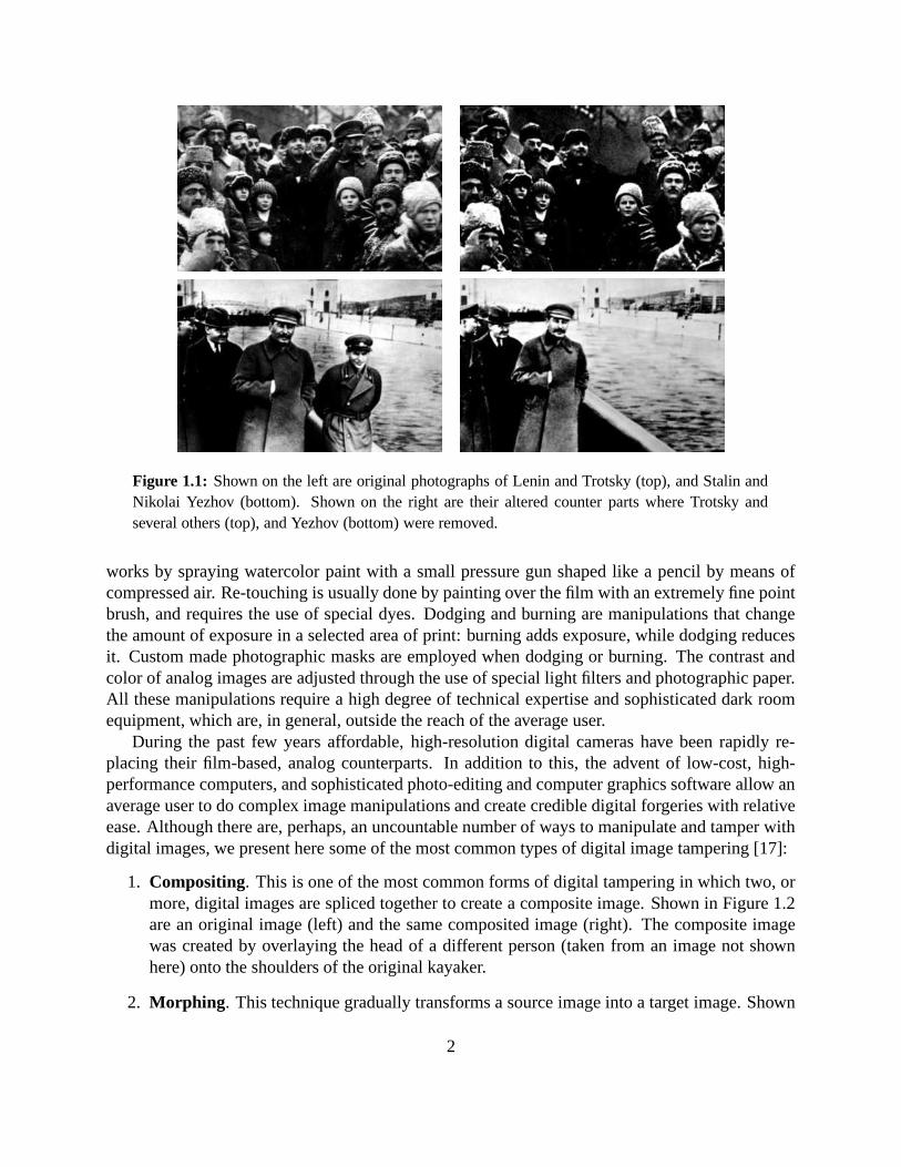
Figure 1.1: Shown on the left are original photographs of Lenin and Trotsky (top), and Stalin andNikolai Yezhov (bottom). Shown on the right are their altered counter parts where Trotsky andseveral others (top), and Yezhov (bottom) were removed.

works by spraying watercolor paint with a small pressure gun shaped like a pencil by means ofcompressed air. Re-touching is usually done by painting over the film with an extremely fine pointbrush, and requires the use of special dyes. Dodging and burning are manipulations that changethe amount of exposure in a selected area of print: burning adds exposure, while dodging reducesit. Custom made photographic masks are employed when dodging or burning. The contrast andcolor of analog images are adjusted through the use of special light filters and photographic paper.All these manipulations require a high degree of technical expertise and sophisticated dark roomequipment, which are, in general, outside the reach of the average user.

During the past few years affordable, high-resolution digital cameras have been rapidly re-placing their film-based, analog counterparts. In addition to this, the advent of low-cost, high-performance computers, and sophisticated photo-editing and computer graphics software allow anaverage user to do complex image manipulations and create credible digital forgeries with relativeease. Although there are, perhaps, an uncountable number of ways to manipulate and tamper withdigital images, we present here some of the most common types of digital image tampering [17]:

1. Compositing. This is one of the most common forms of digital tampering in which two, ormore, digital images are spliced together to create a composite image. Shown in Figure 1.2are an original image (left) and the same composited image (right). The composite imagewas created by overlaying the head of a different person (taken from an image not shownhere) onto the shoulders of the original kayaker.

2. Morphing. This technique gradually transforms a source image into a target image. Shown

2

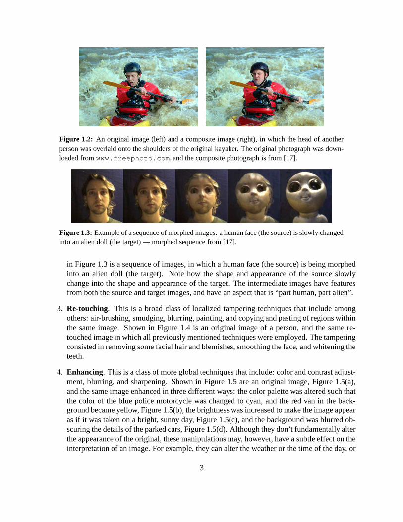
Figure 1.2: An original image (left) and a composite image (right), in which the head of anotherperson was overlaid onto the shoulders of the original kayaker. The original photograph was down-loaded from www.freephoto.com, and the composite photograph is from [17].

Figure 1.3: Example of a sequence of morphed images: a human face (the source) is slowly changedinto an alien doll (the target) — morphed sequence from [17].

in Figure 1.3 is a sequence of images, in which a human face (the source) is being morphedinto an alien doll (the target). Note how the shape and appearance of the source slowlychange into the shape and appearance of the target. The intermediate images have featuresfrom both the source and target images, and have an aspect that is “part human, part alien”.

3. Re-touching. This is a broad class of localized tampering techniques that include amongothers: air-brushing, smudging, blurring, painting, and copying and pasting of regions withinthe same image. Shown in Figure 1.4 is an original image of a person, and the same re-touched image in which all previously mentioned techniques were employed. The tamperingconsisted in removing some facial hair and blemishes, smoothing the face, and whitening theteeth.

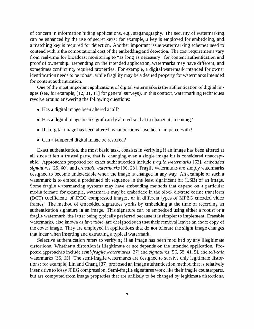
4. Enhancing. This is a class of more global techniques that include: color and contrast adjust-ment, blurring, and sharpening. Shown in Figure 1.5 are an original image, Figure 1.5(a),and the same image enhanced in three different ways: the color palette was altered such thatthe color of the blue police motorcycle was changed to cyan, and the red van in the back-ground became yellow, Figure 1.5(b), the brightness was increased to make the image appearas if it was taken on a bright, sunny day, Figure 1.5(c), and the background was blurred ob-scuring the details of the parked cars, Figure 1.5(d). Although they don’t fundamentally alterthe appearance of the original, these manipulations may, however, have a subtle effect on theinterpretation of an image. For example, they can alter the weather or the time of the day, or

3

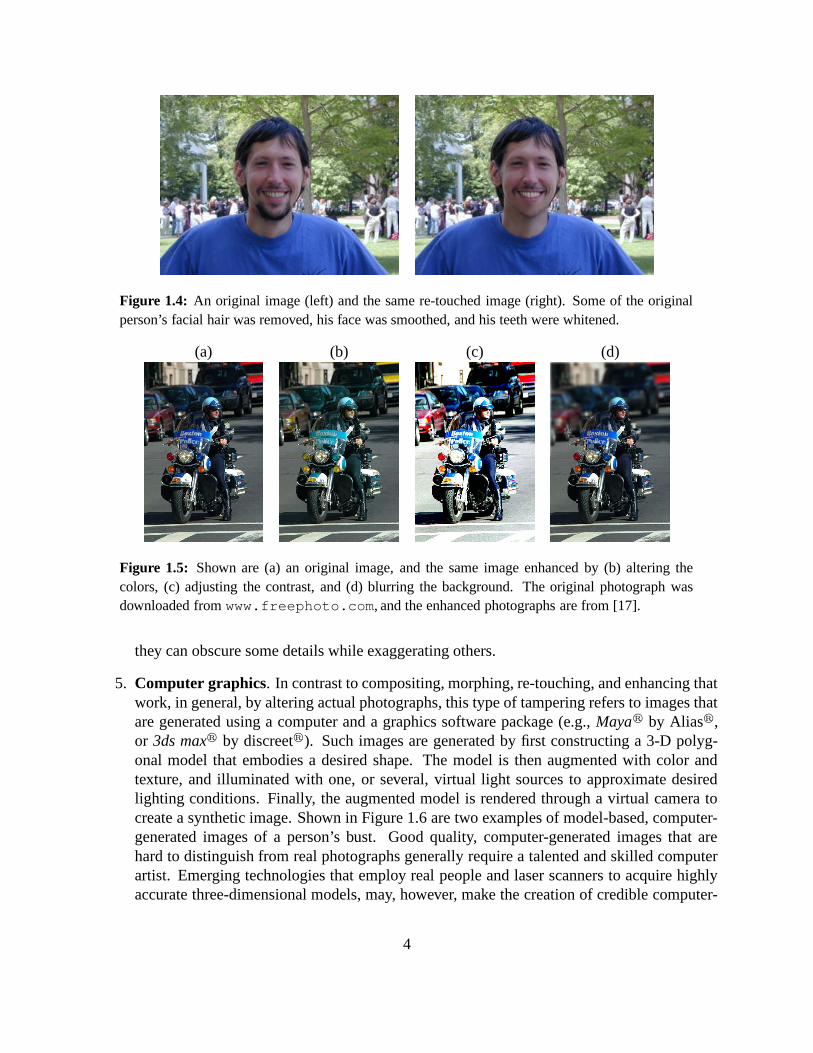
Figure 1.4: An original image (left) and the same re-touched image (right). Some of the originalperson’s facial hair was removed, his face was smoothed, and his teeth were whitened.

(a) (b) (c) (d)

Figure 1.5: Shown are (a) an original image, and the same image enhanced by (b) altering thecolors, (c) adjusting the contrast, and (d) blurring the background. The original photograph wasdownloaded from www.freephoto.com, and the enhanced photographs are from [17].

they can obscure some details while exaggerating others.

5. Computer graphics. In contrast to compositing, morphing, re-touching, and enhancing thatwork, in general, by altering actual photographs, this type of tampering refers to images thatare generated using a computer and a graphics software package (e.g., Mayar by Aliasr,or 3ds maxr by discreetr). Such images are generated by first constructing a 3-D polyg-onal model that embodies a desired shape. The model is then augmented with color andtexture, and illuminated with one, or several, virtual light sources to approximate desiredlighting conditions. Finally, the augmented model is rendered through a virtual camera tocreate a synthetic image. Shown in Figure 1.6 are two examples of model-based, computer-generated images of a person’s bust. Good quality, computer-generated images that arehard to distinguish from real photographs generally require a talented and skilled computerartist. Emerging technologies that employ real people and laser scanners to acquire highlyaccurate three-dimensional models, may, however, make the creation of credible computer-

4

Figure 1.6: Two examples of model-based, computer-generated images of a per-son’s bust. These images were created by Mihai Anghelescu, and downloaded fromwww.xmg.ro/mihai/index.html.

generated images easier and more accessible to less skilled people. A recent trend of interestin the context of digital forgeries, has been the creation of hybrid images that mix real andcomputer-generated images. For example, computer-generated images can be spliced intoreal photographs, and real images can be mapped directly onto a three-dimensional model, atechnique known as image-based rendering.

6. Painted. This type of tampering refers to images created from a blank screen with a photo-editing or drawing software (e.g., Adobe Photoshopr or Corel Drawr) in a way similar tothat of an artist painting on traditional canvas. This technique is the most challenging formof tampering, and would require a highly talented painter with good technical skills to yieldrealistic images.

Note that, when creating digital forgeries, the image manipulations presented above, and others,are often employed simultaneously. For example, two images may be spliced together, then thecomposite image may be re-touched and enhanced. Note also that tampering is not a well definednotion, and is often application dependent. Certain image manipulations may be legitimate in somecases, and illegitimate in others. For example, it may be acceptable to use a composite image for amagazine cover, but not as evidence in a court of law.

5

1.2 Watermarking

Watermarking has been defined [11] as “the practice of imperceptibly2 altering a Work to embed amessage about that Work”, where Work refers to a specific image, audio clip, video clip, or otherdigital media. The basic approach employs an embedder that inserts an imperceptible watermark(e.g., a digital code, or a checksum) into the media, and a decoder that tries to determine if awatermark is present, and if so, outputs its encoded message.

Digital watermarking has many applications, including: broadcast monitoring, owner identifi-cation, proof of ownership, transaction tracking, content authentication, and copy and device con-trol. Although not the only solution for these applications, digital watermarks are distinguishedfrom other techniques by three defining characteristics: (1) they are imperceptible, (2) they areinseparable from the digital media they are embedded in, and (3) they undergo the same transfor-mations as the digital media itself.

Watermarking systems can be characterized by a number of defining properties related to theembedding process (effectiveness, fidelity, and data payload), the detection process (blind vs. in-formed, false positives, and robustness), the security and use of secret keys, and the cost of em-bedding and detection. The embedding effectiveness is the probability of the watermark detectionimmediately after embedding. Although 100% effectiveness is desirable, it may not be always pos-sible without compromising other desirable properties, e.g. fidelity. The fidelity of a watermarkingscheme refers to the perceptual difference between the original and the watermarked media. Ide-ally, watermark embedding should not alter the perception of the cover media. Data payload isthe number of bits that a watermark embeds in a unit of time or within a cover medium. Re-quirements for payload can vary from one bit (a watermark may be present or absent) to severalthousand if, for example, error correction codes need to be embedded. Informed detection refersto watermarking schemes that require access to the original cover medium (or to some informationderived from the original), while blind detection refers to schemes that do not need the original.Blind detection is employed by a majority of watermarking schemes. The false positive rate isthe probability of detecting a watermark in a medium that does not contain one. The require-ments for the false positive rate are application dependent and can vary from 10−6 for proof ofownership, to one in 1012 frames for DVD video. Robustness refers to the ability of a watermarkto survive common signal processing operations, e.g., filtering, lossy compression, printing andscanning, and temporal and geometric distortions. In practice, watermarks are required to surviveonly a specific subset of signal processing operations. The security of a watermark refers to itscapability to resist hostile attacks. Attacks on watermarking schemes typically consist of unau-thorized removal, embedding, or detection. The unauthorized removal refers to active attacks thatprevent the detectability of a watermark either by masking or by eliminating it. The unauthorizedembedding, also known as forgery, refers to the capability of an adversary to insert a watermarkinto a medium with the goal to falsely authenticate it. Unauthorized detection, a passive attack, is

2Imperceptibility is not considered by some researchers as a defining characteristic of digital watermarks, andperceptible watermarking is an active area of research (e.g., [44]). Perceptible watermarks, while useful in conveyingan immediate claim of ownership, eliminate the potential commercial value of the media they are embedded in, whichrestricts their area of applicability.

6

of concern in information hiding applications, e.g., steganography. The security of watermarkingcan be enhanced by the use of secret keys: for example, a key is employed for embedding, anda matching key is required for detection. Another important issue watermarking schemes need tocontend with is the computational cost of the embedding and detection. The cost requirements varyfrom real-time for broadcast monitoring to “as long as necessary” for content authentication andproof of ownership. Depending on the intended application, watermarks may have different, andsometimes conflicting, required properties. For example, a digital watermark intended for owneridentification needs to be robust, while fragility may be a desired property for watermarks intendedfor content authentication.

One of the most important applications of digital watermarks is the authentication of digital im-ages (see, for example, [12, 31, 11] for general surveys). In this context, watermarking techniquesrevolve around answering the following questions:

• Has a digital image been altered at all?

• Has a digital image been significantly altered so that to change its meaning?

• If a digital image has been altered, what portions have been tampered with?

• Can a tampered digital image be restored?

Exact authentication, the most basic task, consists in verifying if an image has been altered atall since it left a trusted party, that is, changing even a single image bit is considered unaccept-able. Approaches proposed for exact authentication include fragile watermarks [63], embeddedsignatures [25, 60], and erasable watermarks [30, 23]. Fragile watermarks are simply watermarksdesigned to become undetectable when the image is changed in any way. An example of such awatermark is to embed a predefined bit sequence in the least significant bit (LSB) of an image.Some fragile watermarking systems may have embedding methods that depend on a particularmedia format: for example, watermarks may be embedded in the block discrete cosine transform(DCT) coefficients of JPEG compressed images, or in different types of MPEG encoded videoframes. The method of embedded signatures works by embedding at the time of recording anauthentication signature in an image. This signature can be embedded using either a robust or afragile watermark, the latter being typically preferred because it is simpler to implement. Erasablewatermarks, also known as invertible, are designed such that their removal leaves an exact copy ofthe cover image. They are employed in applications that do not tolerate the slight image changesthat incur when inserting and extracting a typical watermark.

Selective authentication refers to verifying if an image has been modified by any illegitimatedistortions. Whether a distortion is illegitimate or not depends on the intended application. Pro-posed approaches include semi-fragile watermarks [37] and signatures [56, 58, 41, 5], and tell-talewatermarks [35, 65]. The semi-fragile watermarks are designed to survive only legitimate distor-tions: for example, Lin and Chang [37] proposed an image authentication method that is relativelyinsensitive to lossy JPEG compression. Semi-fragile signatures work like their fragile counterparts,but are computed from image properties that are unlikely to be changed by legitimate distortions,

7

e.g., perceptually significant components such as the low frequency block DCT coefficients. Tell-tale watermarks are robust watermarks that survive tampering, but are distorted in the process. Theanalysis of a distorted tell-tale watermark can then reveal the tampering and distortion type.

Many watermarking systems are designed with the ability to identify not only if an image wasaltered, but to localize the tampering as well, a capability referred to as localization. Most local-ization approaches rely on some form of block-wise [61, 21, 8], or pixel-wise [64] authentication.For example, Yeung and Mintzer [64] have proposed a method that employs a pseudo-randommapping from pixel intensities to binary values. The encoder changes the pixel intensities suchthat the pseudo-random mapping would yield a desired binary pattern, e.g., a tiled, binary imagein the form of a logo. In addition to block and pixel-wise authentication, tell-tale watermarks mayalso have the localization capability.

Restoration refers to the ability of a watermarking scheme to restore image regions that havebeen corrupted. One possible approach is to embed redundant information in the image, e.g., errordetection and correction codes. Although this approach allows perfect restoration, it is, however,impractical as the amount of information to be embedded is significant. More practical approaches,self-embedding [22, 38] and blind restoration [33, 34], allow only approximate restoration. Self-embedding works by embedding a highly compressed version of an image into itself: for example,a low quality, lossy compressed version of a given image can be embedded into the least significantbits of its own pixels. Blind restoration employs a tell-tale watermark to determine what distortionshave been applied to an image, then attempts to invert those distortions.

A recent approach to implement a secure digital camera has been proposed by Blythe andFridrich [7]. The method works by first collecting biometric data of the camera user, crypto-graphic hashes of the camera scene, the date and time, and other forensic data. This informationis then inserted into the image using an invisible, erasable watermark (the image is left intact afterthe watermark extraction). The whole procedure links the photographer to the photograph, in ad-dition to providing protection to tampering, and may prove to be useful for investigations by lawenforcement examiners.

A major drawback of watermarking-based approaches is that the watermarks must be insertedeither at the time of recording, or afterward by a person authorized to do so, which requires spe-cially equipped cameras or subsequent processing of the original image. These methods also relyon the assumption that it is difficult to remove and reinsert digital watermarks in images. It isunclear if this is a reasonable assumption (e.g., [13]).

1.3 Related Work

Detecting digital tampering in the absence of watermarks or signatures is a relatively new researchtopic, and only few results have been published so far. Farid [16] proposed a technique for au-thenticating digital audio signals. This technique works under the assumption that natural signalshave low higher-order correlations in the frequency domain. He then showed that higher-ordercorrelations are introduced in the frequency domain when a natural audio signal undergoes a non-linear transformation, as would likely happen in the process of creating a digital forgery. Tools

8

from polyspectral analysis, i.e., the bispectrum, were applied to quantify and detect these correla-tions. This approach was extended by Ng and Chang [47] to detect splicing in composite images.Farid and Popescu have also applied this technique to blindly detect the presence of multiple non-linearities in digital images [51], which represents a possible sign of tampering.

Lyu and Farid [40] have proposed a method to distinguish between photographic and computer-generated, photo-realistic images. Their method works by representing an image with a multi-scale, multi-resolution, wavelet-like transform, then extracting a feature vector of first and higher-order statistics from the transform coefficients. Statistical learning tools (e.g., linear discriminantanalysis and non-linear support vector machines) are employed on these feature vectors to discrim-inate between photographic and photo-realistic images.

Fridrich et al. [24] have proposed a method to detect duplicated regions in digital images. Thismethod, similar to the one we propose in Chapter 5, works by lexicographically sorting the DCTcoefficients of fixed-size image blocks, and examining neighboring blocks in the sorted order.Similar neighboring blocks are then employed to highlight the potential duplicated regions in theimage.

1.4 Contributions

We describe a set of statistical techniques for detecting traces of tampering in digital images. Thesetechniques work in the complete absence of any digital watermark or signature. The commontheme, and unifying framework, of these techniques is the assumption that digital forgeries, oftenvisually imperceptible, alter some underlying statistical properties of natural images. Within thisframework, our approach consists in first identifying the statistical changes associated with partic-ular kinds of tampering, then designing techniques for estimating these changes. Following thisapproach, we have developed five techniques that quantify and detect different types of tampering:

1. Re-sampled Images. Imagine a forgery created by splicing together images of two peopleand overlaying them on a chosen background. In order to create a convincing match it isoften necessary to re-size, rotate, or stretch the original images (or portions of them), whichrequires re-sampling the images onto a different lattice. Re-sampling introduces specificcorrelations between neighboring image pixels, that are quantified and detected using theexpectation-maximization (EM) algorithm.

2. Manipulated Color Filter Array (CFA) Interpolated Images. Most digital cameras areequipped with a single charge-coupled device (CCD) or complementary metal oxide semi-conductor (CMOS) sensor, and capture color images using an array of color filters. At eachpixel location, only a single color sample (out of three) is captured. The missing color sam-ples are then inferred from neighboring values. This process, known as CFA interpolationor demosaicking, introduces specific correlations between the samples of a color image.These correlations are typically destroyed when a CFA interpolated image is tampered with,and can be employed to uncover traces of tampering. Using an approach similar to the re-sampling detection, we have employed the EM algorithm to detect if the CFA interpolationcorrelations are missing in any portion of an image.

9

3. Double JPEG Compression. When tampering with an image, a typical pattern is to load theimage into a photo-editing software (e.g., Adobe Photoshopr), do some processing, and re-save the tampered image. If JPEG format is used to store the images, the resulting tamperedimage has been double compressed. Double JPEG compression introduces specific corre-lations between the discrete cosine transform (DCT) coefficients of image blocks. Thesecorrelations can be detected and quantified by examining the histograms of the DCT coeffi-cients. While double JPEG compression of an image does not necessarily prove malicioustampering, it raises suspicions that the image may not be authentic.

4. Duplicated Image Regions. A common manipulation in removing an unwanted person orobject from an image, is to copy and paste portions of the same image over the desired re-gion. If the splicing is imperceptible, little concern is typically given to the fact that identicalregions are present in the image. We have developed an algorithm that employs a principalcomponent analysis (PCA) on fixed-size image blocks, and lexicographic sorting to effi-ciently detect the presence of duplicated regions even in noisy or lossy compressed images.

5. Inconsistent Noise Patterns. Digital images contain an inherent amount of noise that islargely uniformly distributed across an entire image. When creating digital forgeries, it iscommon to add small amounts of localized noise to tampered regions in order to concealtraces of tampering (e.g., at a splice boundary). As a result, local noise levels across theimage may become inconsistent. We have implemented an algorithm for blind estimation oflocalized noise variance, and employed it to differentiate regions with different amounts ofadditive noise.

For each of the above techniques, we develop its theoretical foundation, show its effectiveness indetecting credible forgeries, and analyze its sensitivity and robustness to simple counter-attacks.

10

Chapter 2

Re-sampled Images

Consider the scenario in which a digital forgery is created by splicing together two or more images.In order to create a convincing match, it is often necessary to re-size, rotate, or stretch the images,or portions of them. This procedure typically requires re-sampling an image onto a new samplinglattice using an interpolation technique (e.g., bi-cubic). Although a re-sampled image is oftenimperceptible, it contains specific correlations that, when detected, may represent evidence oftampering. We describe the form of these correlations, and propose an algorithm for detectingthem in any portion of an image.

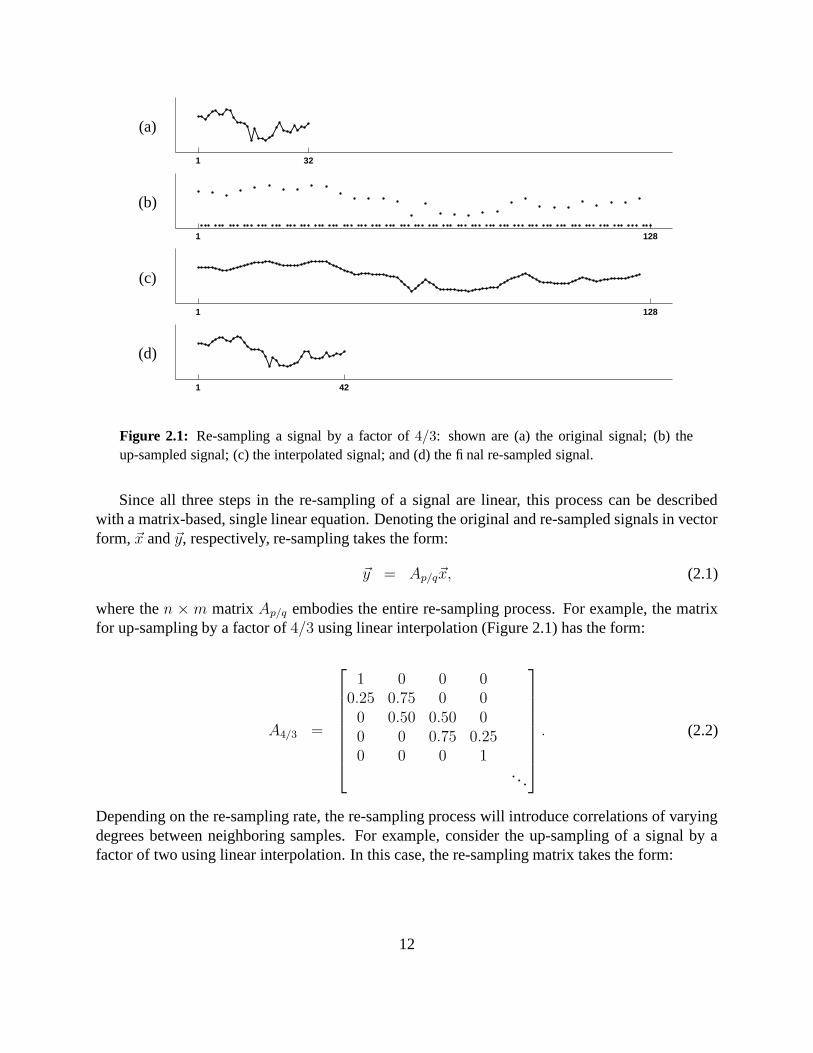
For purposes of exposition we will first describe how and where re-sampling introduces corre-lations in 1-D signals, and how to detect these correlations. The relatively straightforward gener-alization to 2-D images is then presented. To illustrate the general effectiveness of this technique,we show results on re-sampled natural test images and on perceptually credible forgeries. Alsopresented is an extensive set of experiments that test the sensitivity of re-sampling detection for alarge set of parameters, as well as the technique’s robustness to simple counter-attacks and lossyimage compression schemes.

2.1 Re-sampling Signals

Consider a 1-D discretely-sampled signal x[t] with m samples, Figure 2.1(a). The number ofsamples in this signal can be increased or decreased by a factor p/q to n samples in three steps [48]:

1. up-sample: create a new signal xu[t] with pm samples, where xu[pt] = x[t], t = 1, 2, ..., m,and xu[t] = 0 otherwise, Figure 2.1(b).

2. interpolate: convolve xu[t] with a low-pass filter: xi[t] = xu[t] ? h[t], Figure 2.1(c).

3. down-sample: create a new signal xd[t] with n samples, where xd[t] = xi[qt], t = 1, 2, ..., n.Denote the re-sampled signal as y[t] ≡ xd[t], Figure 2.1(d).

Different types of re-sampling algorithms (e.g., linear, cubic [32]) differ in the form of the interpo-lation filter h[t] in step 2.

11

(a)

1 32

(b)

1 128

(c)

1 128

(d)

1 42

Figure 2.1: Re-sampling a signal by a factor of 4/3: shown are (a) the original signal; (b) theup-sampled signal; (c) the interpolated signal; and (d) the final re-sampled signal.

Since all three steps in the re-sampling of a signal are linear, this process can be describedwith a matrix-based, single linear equation. Denoting the original and re-sampled signals in vectorform, ~x and ~y, respectively, re-sampling takes the form:

~y = Ap/q~x, (2.1)

where the n × m matrix Ap/q embodies the entire re-sampling process. For example, the matrixfor up-sampling by a factor of 4/3 using linear interpolation (Figure 2.1) has the form:

A4/3 =

1 0 0 00.25 0.75 0 00 0.50 0.50 00 0 0.75 0.250 0 0 1

. . .

. (2.2)

Depending on the re-sampling rate, the re-sampling process will introduce correlations of varyingdegrees between neighboring samples. For example, consider the up-sampling of a signal by afactor of two using linear interpolation. In this case, the re-sampling matrix takes the form:

12

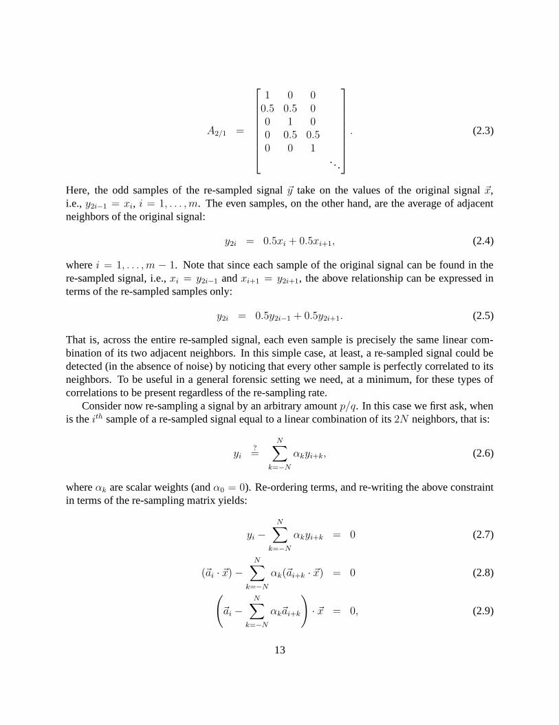
A2/1 =

1 0 00.5 0.5 00 1 00 0.5 0.50 0 1

. . .

. (2.3)

Here, the odd samples of the re-sampled signal ~y take on the values of the original signal ~x,i.e., y2i−1 = xi, i = 1, . . . , m. The even samples, on the other hand, are the average of adjacentneighbors of the original signal:

y2i = 0.5xi + 0.5xi+1, (2.4)

where i = 1, . . . , m − 1. Note that since each sample of the original signal can be found in there-sampled signal, i.e., xi = y2i−1 and xi+1 = y2i+1, the above relationship can be expressed interms of the re-sampled samples only:

y2i = 0.5y2i−1 + 0.5y2i+1. (2.5)

That is, across the entire re-sampled signal, each even sample is precisely the same linear com-bination of its two adjacent neighbors. In this simple case, at least, a re-sampled signal could bedetected (in the absence of noise) by noticing that every other sample is perfectly correlated to itsneighbors. To be useful in a general forensic setting we need, at a minimum, for these types ofcorrelations to be present regardless of the re-sampling rate.

Consider now re-sampling a signal by an arbitrary amount p/q. In this case we first ask, whenis the ith sample of a re-sampled signal equal to a linear combination of its 2N neighbors, that is:

yi?=

N∑

k=−N

αkyi+k, (2.6)

where αk are scalar weights (and α0 = 0). Re-ordering terms, and re-writing the above constraintin terms of the re-sampling matrix yields:

yi −N∑

k=−N

αkyi+k = 0 (2.7)

(~ai · ~x) −N∑

k=−N

αk(~ai+k · ~x) = 0 (2.8)

(

~ai −N∑

k=−N

αk~ai+k

)

· ~x = 0, (2.9)

13

where ~ai is the ith row of the re-sampling matrix Ap/q, and ~x is the original signal. We see nowthat the ith sample of a re-sampled signal is equal to a linear combination of its neighbors whenthe ith row of the re-sampling matrix, ~ai, is equal to a linear combination of the neighboring rows,∑N

k=−N αk~ai+k. For example, in the case of up-sampling by a factor of two, Equation (2.3), theeven rows are a linear combination of the two adjacent odd rows. Note also that if the ith sampleis a linear combination of its neighbors then the (i − kp)th sample (k an integer) will be the samecombination of its neighbors, that is, the correlations are periodic. It is, of course, possible for theconstraint of Equation (2.9) to be satisfied when the difference on the left-hand side of the equationis orthogonal to the original signal ~x. While this may occur on occasion, these correlations areunlikely to be periodic.

2.2 Detecting Re-sampling

Given a signal that has been re-sampled by a known amount and interpolation method, it is possibleto find a set of periodic samples that are correlated in the same way to their neighbors. For example,consider again the re-sampling matrix of Equation (2.2). Here, based on the periodicity of the re-sampling matrix, we see that, for example, the 3rd, 7th, 11th, etc. samples of the re-sampled signalwill have the same correlations to their neighbors. The specific form of the correlations can bedetermined by finding the neighborhood size, N , and the set of coefficients, ~α, that satisfy: ~ai =∑N

k=−N αk~ai+k, Equation (2.9), where ~ai is the ith row of the re-sampling matrix and i = 3, 7, 11,etc. If, on the other-hand, we know the specific form of the correlations, ~α, then it is straightforwardto determine which samples satisfy yi =

∑Nk=−N αkyi+k, Equation (2.7).

In practice, of course, neither the samples that are correlated, nor the specific form of thecorrelations are known. In order to determine if a signal has been re-sampled, we employ theexpectation-maximization algorithm1 (EM) [14] to simultaneously estimate a set of periodic sam-ples that are correlated to their neighbors, and the specific form of these correlations. We beginby assuming that each sample belongs to one of two models. The first model, M1, corresponds tothose samples yi that are correlated to their neighbors, i.e., are generated according to the followingmodel:

M1 : yi =N∑

k=−N

αkyi+k + n(i), (2.10)

where the model parameters are given by the specific form of the correlations, ~α (α0 = 0), andn(i) denote independently, and identically distributed (i.i.d.) samples drawn from a Gaussian dis-tribution with zero mean and unknown variance σ2. The second model, M2, corresponds to thosesamples that are not correlated to their neighbors, i.e., are generated by an outlier process. TheEM algorithm is a two-step iterative algorithm: (1) in the E-step the probability that each samplebelongs to each model is estimated; and (2) in the M-step the specific form of the correlationsbetween samples is estimated. More specifically, in the E-step, the probability of each sample yi

1A short tutorial on the general EM algorithm, and an example of its application to a mixture models problem arepresented in Appendix A.

14

belonging to model M1 can be obtained using Bayes’ rule:

Pr{yi ∈ M1 | yi} =Pr{yi | yi ∈ M1}Pr{yi ∈ M1}

∑2k=1 Pr{yi | yi ∈ Mk}Pr{yi ∈ Mk}

, (2.11)

where the priors Pr{yi ∈ M1} and Pr{yi ∈ M2} are assumed to be equal to 1/2. The probabilityof observing a sample yi knowing it was generated by model M1 is given by:

Pr{yi | yi ∈ M1} =1

σ√

2πexp

−(

yi −∑N

k=−N αkyi+k

)2

2σ2

. (2.12)

We assume that the probability of observing samples generated by the outlier model, Pr{yi | yi ∈M2}, is uniformly distributed over the range of possible values of yi. The variance, σ2, of theGaussian distribution in Equation (2.12) is estimated in the M-step (see Section 2.6). Note that theE-step requires an estimate of ~α, which on the first iteration is chosen randomly. In the M-step,a new estimate of ~α is computed using weighted least-squares, that is, minimizing the followingquadratic error function:

E(~α) =∑

i

w(i)

(

yi −N∑

k=−N

αkyi+k

)2

, (2.13)

where the weights w(i) ≡ Pr{yi ∈ M1 | yi}, Equation (2.11), and α0 = 0. This error functionis minimized by computing the gradient with respect to ~α, and setting the result equal to zero.Solving for ~α yields:

~α = (Y T WY )−1Y T W~y, (2.14)

where the matrix Y is:

Y =

y1 . . . yN yN+2 . . . y2N+1

y2 . . . yN+1 yN+3 . . . y2N+2...

......

...yi . . . yN+i−1 yN+i+1 . . . y2N+i...

......

...

, (2.15)

and W is a diagonal weighting matrix with w(i) along the diagonal.The E-step and the M-step are iteratively executed until a stable estimate of ~α is achieved — see

Section 2.6 for a detailed algorithm. The final ~α has the property that it maximizes the likelihoodof the observed samples2 — see Appendix A for more details on maximum likelihood estimationand EM.

2The EM algorithm is proved to always converge to a stable estimate that is a local maximum of the log-likelihoodof the observed data, [14] and Appendix A.

15

1 32

0.6 1.0 0.6

0.1

0.9 0.5 0.8

0.0

0.8

0.4

1.0 1.0

0.0 0.0 0.0

1.0 1.0 0.7 0.7

0.5

1.0

0.0

1.0 1.0

0.1 0.0

0.8 0.7

1 42

1.0

0.0 0.0 0.0

1.0

0.0 0.0 0.0

1.0

0.0 0.0 0.0

1.0

0.0 0.0 0.0

1.0

0.0 0.0 0.0

1.0

0.0 0.0 0.0

1.0

0.0 0.0 0.0

1.0

0.0 0.0 0.0

1.0

0.0 0.0 0.0

1.0

0.0

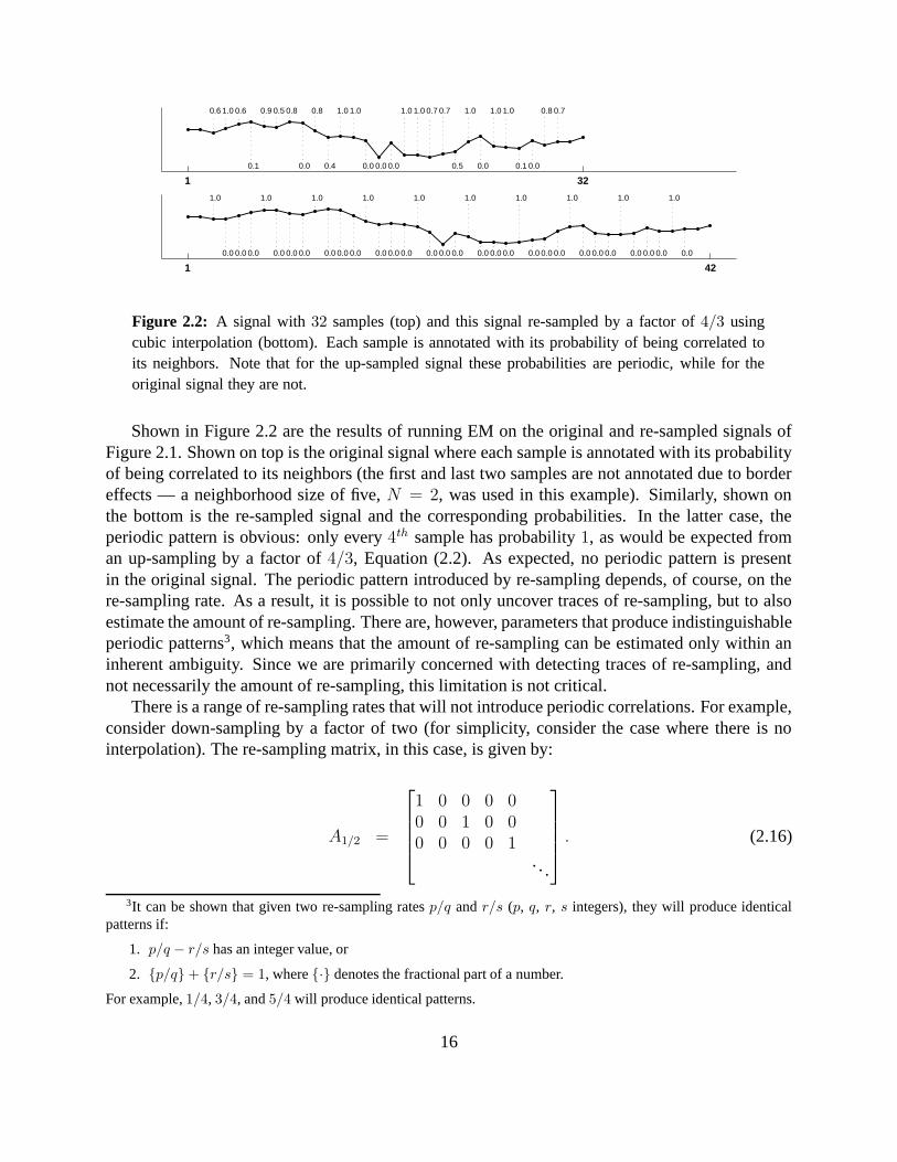
Figure 2.2: A signal with 32 samples (top) and this signal re-sampled by a factor of 4/3 usingcubic interpolation (bottom). Each sample is annotated with its probability of being correlated toits neighbors. Note that for the up-sampled signal these probabilities are periodic, while for theoriginal signal they are not.

Shown in Figure 2.2 are the results of running EM on the original and re-sampled signals ofFigure 2.1. Shown on top is the original signal where each sample is annotated with its probabilityof being correlated to its neighbors (the first and last two samples are not annotated due to bordereffects — a neighborhood size of five, N = 2, was used in this example). Similarly, shown onthe bottom is the re-sampled signal and the corresponding probabilities. In the latter case, theperiodic pattern is obvious: only every 4th sample has probability 1, as would be expected froman up-sampling by a factor of 4/3, Equation (2.2). As expected, no periodic pattern is presentin the original signal. The periodic pattern introduced by re-sampling depends, of course, on there-sampling rate. As a result, it is possible to not only uncover traces of re-sampling, but to alsoestimate the amount of re-sampling. There are, however, parameters that produce indistinguishableperiodic patterns3, which means that the amount of re-sampling can be estimated only within aninherent ambiguity. Since we are primarily concerned with detecting traces of re-sampling, andnot necessarily the amount of re-sampling, this limitation is not critical.

There is a range of re-sampling rates that will not introduce periodic correlations. For example,consider down-sampling by a factor of two (for simplicity, consider the case where there is nointerpolation). The re-sampling matrix, in this case, is given by:

A1/2 =

1 0 0 0 00 0 1 0 00 0 0 0 1

. . .

. (2.16)

3It can be shown that given two re-sampling rates p/q and r/s (p, q, r, s integers), they will produce identicalpatterns if:

1. p/q − r/s has an integer value, or

2. {p/q} + {r/s} = 1, where {·} denotes the fractional part of a number.

For example, 1/4, 3/4, and 5/4 will produce identical patterns.

16

Note that no row can be written as a linear combination of neighboring rows (the rows are orthogo-nal to one another), and that, in this case, re-sampling is not detectable. In general, the detectabilityof any re-sampling can be determined by generating the re-sampling matrix, and checking whetherany rows can be expressed as a linear combination of neighboring rows.

2.3 Re-sampling Images

In the previous sections we showed that for 1-D signals re-sampling introduces periodic correla-tions, and that these correlations can be detected using the EM algorithm. The extension to 2-Dimages is relatively straightforward. As with 1-D signals, the up-sampling or down-sampling, ofan image is still linear and involves the same three steps: up-sampling, interpolation, and down-sampling — these steps are simply carried out on a 2-D lattice. Again, as with 1-D signals, there-sampling of an image introduces periodic correlations. Though we will only show this for up-and down-sampling, the same is true for an arbitrary affine transform4.

Consider, for example, the simple case of up-sampling by a factor of two. Shown in Figure 2.3are, from left to right, a portion of an original 2-D sampling lattice, the same lattice up-sampled bya factor of two, and a subset of the pixels of the re-sampled image. Assuming linear interpolation,these pixels are given by:

y2 = 0.5y1 + 0.5y3

y4 = 0.5y1 + 0.5y7

y5 = 0.25y1 + 0.25y3 + 0.25y7 + 0.25y9,

(2.17)

and where y1 = x1, y3 = x2, y7 = x3, y9 = x4. Note that the pixels of the re-sampled imagein the odd rows and even columns (e.g., y2) will all be the same linear combination of their twohorizontal neighbors. Similarly, the pixels of the re-sampled image in the even rows and oddcolumns (e.g., y4) will all be the same linear combination of their two vertical neighbors. That is,as with 1-D signals, the correlations due to re-sampling are periodic. A 2-D version of the EMalgorithm can then be applied to uncover these correlations in images.

2.4 Results

For the results presented here, we employed approximately 200 gray-scale images and 50 colorimages in TIFF format, both 512 × 512 pixels in size. Each of these images were cropped from asmaller set of thirty-five 1200× 1600 images taken with a Nikon Coolpix 950 camera (the camerawas set to capture and store in uncompressed TIFF format). Using bi-cubic interpolation theseimages were up-sampled, down-sampled, rotated, or affine transformed by varying amounts.

For the original and re-sampled images, the EM algorithm described in Section 2.2 was usedto estimate probability maps that embody the correlations between pixels and their neighbors. The

4Even non-linear transformations introduce detectable correlations, but these correlations may not be periodic.

17

x1 x2

x3 x4

x1 0 x2

0 0 0

x3 0 x4

y1 y2 y3

y4 y5

y7 y9

Figure 2.3: Shown from left to right are: a portion of the 2D lattice of an image, the same latticeup-sampled by a factor of 2, and a portion of the lattice of the re-sampled image.

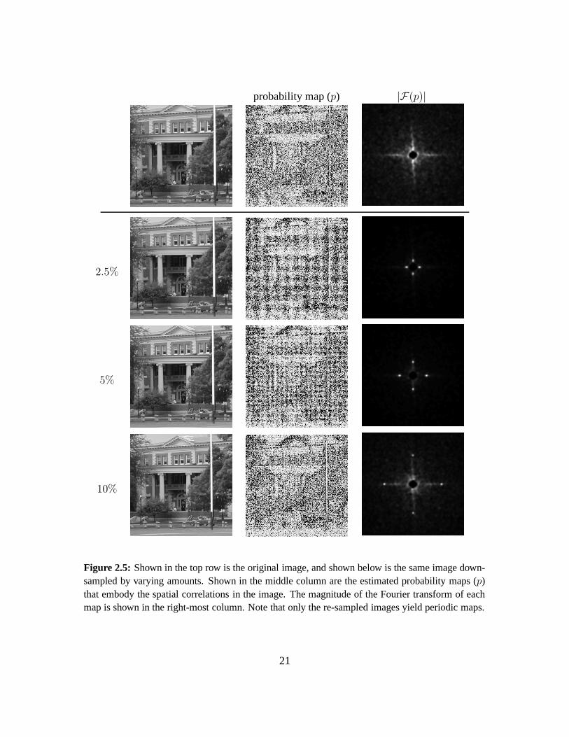
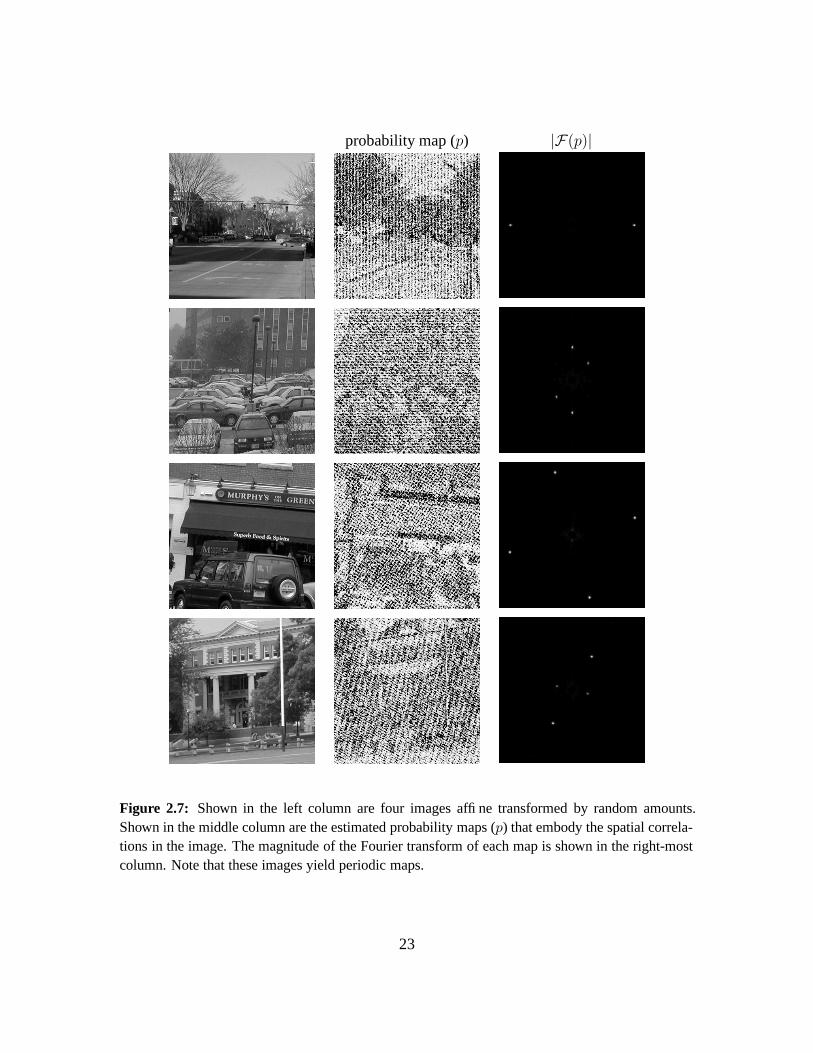
EM parameters were fixed throughout at N = 2, σ0 = 0.0075, Nh = 3 5, and p0 = 1/256 (seeSection 2.6). Shown in Figures 2.4-2.6 are several examples of the periodic patterns that emergeddue to re-sampling. In the top row of each figure are (from left to right) the original image, theestimated probability map and the magnitude of the central portion of the Fourier transform ofthis map (for display purposes, each Fourier transform was independently auto-scaled to fill thefull intensity range and high-pass filtered to remove the lowest frequencies). Shown below thisrow is the same image uniformly re-sampled at different rates. For the re-sampled images, notethe periodic nature of their probability maps and the strong, localized peaks in their correspondingFourier transforms. Shown in Figure 2.7 are examples of the periodic patterns that emerge fromfour different affine transforms.

Shown in Figure 2.8 are results from applying consecutive re-samplings. Specifically, theimage in the left column is the result of up-sampling by 15% an original image, then rotatingby 5◦ the up-sampled image. The same operations were performed in reverse order on the sameoriginal image to yield the image in the right column. Note that while the images are perceptuallyindistinguishable, the periodic patterns that emerge are quite distinct, with the last re-samplingoperation dominating the pattern. Note also that the corresponding Fourier transforms containseveral sets of peaks corresponding to both re-sampling operations. As with a single re-sampling,consecutive re-samplings can be easily detected.

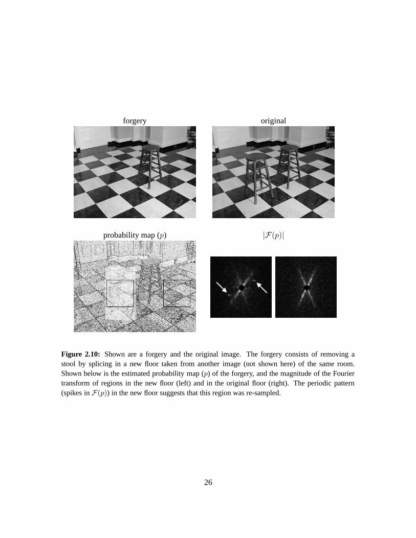
Shown in Figures 2.9-2.11 are several examples of our detection algorithm applied to imageswhere only a portion of the image was re-sampled. Regions in each image were subjected to arange of stretching, rotation, shearing, etc. (these manipulations were done in Adobe Photoshopr).Shown in each figure is the original photograph, the forgery (where a portion of the original isreplaced or altered), and the estimated probability map. Note that in each case, the re-sampledregion is clearly detected — while the periodic patterns are not particularly visible in the spatialdomain at the reduced scale, the well localized peaks in the Fourier domain clearly reveal theirpresence (for display purposes, each Fourier transform was independently auto-scaled to fill the

5The blurring of the residual error with a binomial filter of size Nh × Nh is not critical, but merely accelerates theconvergence.

18

full intensity range and high-pass filtered to suppress the lowest frequencies). Note also that inFigure 2.9 the white sheet of paper on top of the trunk has strong activation in the probability map— when seen in the Fourier domain, however, it is clear that this region is not periodic, but ratheruniform, and thus not representative of a re-sampled region.

2.4.1 Sensitivity and Robustness

From a digital forensic perspective it is important to quantify the robustness and sensitivity ofour detection algorithm. To this end, it is first necessary to devise a quantitative measure of theamount of periodicity found in the estimated probability maps. To do so, we compare the estimatedprobability map with a set of synthetically generated probability maps that contain periodic patternssimilar to those that emerge from re-sampled images.

Quantifying Re-sampling Correlations

Given a set of re-sampling parameters and interpolation method, a synthetic map is generated basedon the periodicity of the re-sampling matrix. There are, however, several possible periodic patternsthat may emerge in a re-sampled image. For example, in the case of up-sampling by a factor oftwo using linear interpolation, Equation (2.17), the coefficients ~α estimated by the EM algorithm(with a 3 × 3 neighborhood) are expected to be one of the following:

~α1 =

0 0.5 00 0 00 0.5 0

~α2 =

0 0 00.5 0 0.50 0 0

~α3 =

0.25 0 0.250 0 0

0.25 0 0.25

. (2.18)

We have observed that EM will return one of these estimates only when the initial value of ~α isclose to one of the above three values, the neighborhood size is 3, and the initial variance of theconditional probability (σ in Equation (2.12)) is relatively small. In general, however, this finetuning of the starting conditions is not practical. To be broadly applicable, we randomly choosean initial value for ~α, and set the neighborhood size and initial value of σ to values that affordconvergence for a broad range of re-sampling parameters. Under these conditions, we have foundthat for specific re-sampling parameters and interpolation method, the EM algorithm typicallyconverges to a unique set of linear coefficients. In the above example of up-sampling by a factorof two the EM algorithm typically converges to:

~α =

−0.25 0.5 −0.250.5 0 0.5

−0.25 0.5 −0.25

. (2.19)

Note that this solution is different than each of the solutions in Equation (2.18). Yet, the relation-ships in Equation (2.17) are still satisfied by this choice of coefficients. Since the EM algorithmtypically converges to a unique set of linear coefficients, there is also a unique periodic patternthat emerges. It is possible to predict this pattern by analyzing the periodic patterns that emergefrom a large set of images. In practice, however, this approach is computationally demanding,

19

probability map (p) |F(p)|

5%

10%

20%

Figure 2.4: Shown in the top row is the original image, and shown below is the same image up-sampled by varying amounts. Shown in the middle column are the estimated probability maps (p)that embody the spatial correlations in the image. The magnitude of the Fourier transform of eachmap is shown in the right-most column. Note that only the re-sampled images yield periodic maps.

20


2.5%

5%

10%

Figure 2.5: Shown in the top row is the original image, and shown below is the same image down-sampled by varying amounts. Shown in the middle column are the estimated probability maps (p)that embody the spatial correlations in the image. The magnitude of the Fourier transform of eachmap is shown in the right-most column. Note that only the re-sampled images yield periodic maps.

21


2◦

5◦

10◦

Figure 2.6: Shown in the top row is the original image, and shown below is the same image rotatedby varying amounts. Shown in the middle column are the estimated probability maps (p) thatembody the spatial correlations in the image. The magnitude of the Fourier transform of eachmap is shown in the right-most column. Note that only the re-sampled images yield periodic maps.

22


Figure 2.7: Shown in the left column are four images affine transformed by random amounts.Shown in the middle column are the estimated probability maps (p) that embody the spatial correla-tions in the image. The magnitude of the Fourier transform of each map is shown in the right-mostcolumn. Note that these images yield periodic maps.

23

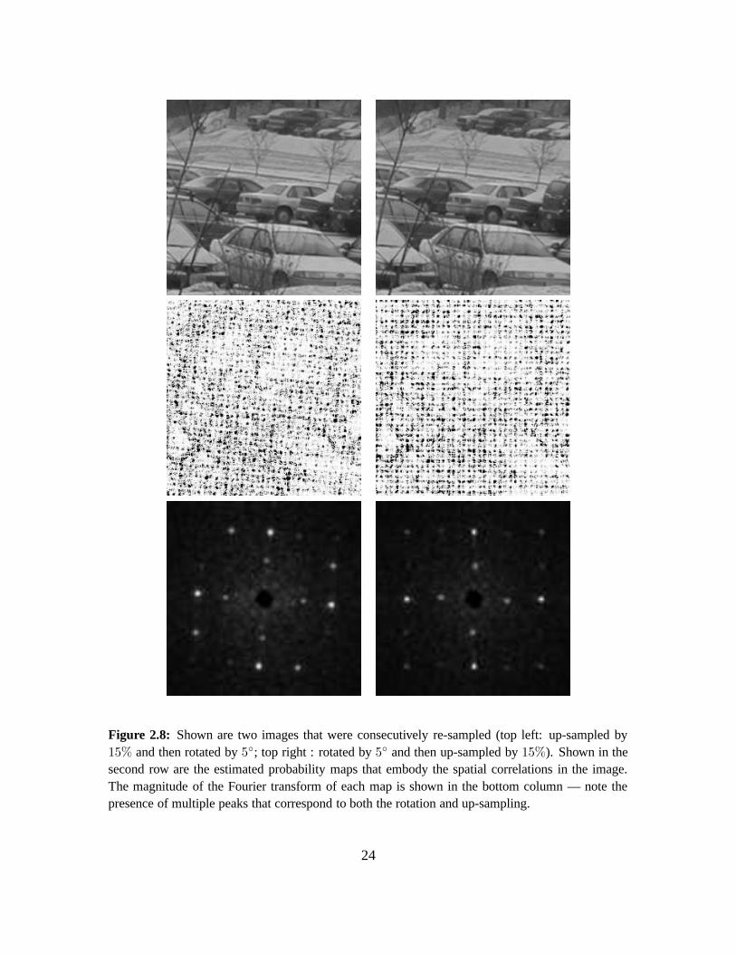
Figure 2.8: Shown are two images that were consecutively re-sampled (top left: up-sampled by15% and then rotated by 5◦; top right : rotated by 5◦ and then up-sampled by 15%). Shown in thesecond row are the estimated probability maps that embody the spatial correlations in the image.The magnitude of the Fourier transform of each map is shown in the bottom column — note thepresence of multiple peaks that correspond to both the rotation and up-sampling.

24

forgery original


Figure 2.9: Shown are a forgery and the original image. The forgery consists of splicing in a newlicense plate number. Shown below is the estimated probability map (p) of the forgery, and themagnitude of the Fourier transform of regions in the license plate (left) and on the car trunk (right).The periodic pattern (spikes in F(p)) in the license plate suggests that this region was re-sampled.

25

forgery original


Figure 2.10: Shown are a forgery and the original image. The forgery consists of removing astool by splicing in a new floor taken from another image (not shown here) of the same room.Shown below is the estimated probability map (p) of the forgery, and the magnitude of the Fouriertransform of regions in the new floor (left) and in the original floor (right). The periodic pattern(spikes in F(p)) in the new floor suggests that this region was re-sampled.

26

forgery original


Figure 2.11: Shown are a forgery and the original image. The forgery consists of widening andshearing the pillars. Shown below is the estimated probability map (p) of the forgery, and themagnitude of the Fourier transform of regions on the pillar (left) and on the building (right). Theperiodic pattern (spikes in F(p)) on the pillar suggests that this region was re-sampled.

27

and therefore we employ a simpler method that was experimentally determined to generate similarperiodic patterns. This method first warps a rectilinear integer lattice according to a specified setof re-sampling parameters. From this warped lattice, the synthetic map is generated by computingthe minimum distance between a warped point and an integer sampling lattice. More specifically,let M denote a general affine transform which embodies a specific re-sampling. Let (x, y) denotethe points on an integer lattice, and (x, y) denote the points of a lattice obtained by warping theinteger lattice (x, y) according to M :

[

xy

]

= M

[

xy

]

. (2.20)

The synthetic map, s(x, y), corresponding to M is generated by computing the minimum distancebetween each point in the warped lattice (x, y) to a point in the integer lattice:

s(x, y) = minx0,y0

√

(x − x0)2 + (y − y0)2, (2.21)

where x0 and y0 are integers, and (x, y) are functions of (x, y) as given in Equation (2.20). Syn-thetic maps generated using this method are similar to the experimentally determined probabilitymaps, Figure 2.12.

The similarity between an estimated probability map, p(x, y), and a synthetic map, s(x, y), iscomputed as follows:

1. The probability map p is Fourier transformed: P (ωx, ωy) = F(p(x, y) ·W (x, y)), where theradial portion of the rotationally invariant window, W (x, y), takes the form:

f(r) =

{

1 0 ≤ r < 3/412

+ 12cos(

π(r−3/4)√2−3/4

)

3/4 ≤ r ≤√

2,(2.22)

where the radial axis is normalized between 0 and√

2. For notational convenience the spatialarguments on p(·) and P (·) will be dropped.

2. The Fourier transformed map P is then high-pass filtered to remove undesired low frequencynoise: PH = P · H , where the radial portion of the rotationally invariant high-pass filter, H ,takes the form:

h(r) =1

2− 1

2cos

(

πr√2

)

, 0 ≤ r ≤√

2. (2.23)

3. The high-passed spectrum PH is then normalized in the [0, 1] range, gamma corrected toenhance frequency peaks, and then rescaled back to its original range:

PG =

(

PH

max(|PH |)

)4

× max(|PH |). (2.24)

28

p

|F(p)|

s

|F(s)|

Figure 2.12: Shown in the first two rows are estimated probability maps, p, from images that werere-sampled (affine transformed), and the magnitude of the Fourier transform of these maps. Notethe strong periodic patterns. Shown in the third and fourth rows are the synthetically generatedprobability maps computed using the same re-sampling parameters — note the similarity to theestimated maps.

29

4. The synthetic map s is simply Fourier transformed: S = F(s).

5. The measure of similarity between p and s is then given by:

M(p, s) =∑

ωx,ωy

|PG(ωx, ωy)| · |S(ωx, ωy)|, (2.25)

where | · | denotes absolute value (note that this similarity measure is phase insensitive).

A set of synthetic probability maps are first generated from a number of different re-samplingparameters. For a given probability map p, the most similar synthetic map, s?, is found through abrute-force search over the entire set: s? = arg maxs M(p, s). If the similarity measure, M(p, s?),is above a specified threshold, then a periodic pattern is assumed to be present in the estimatedprobability map, and the image is classified as re-sampled. This threshold is empirically deter-mined using only the original images in the database to yield a false positive rate less than 1%.

With the ability to quantitatively measure whether an image has been re-sampled, we testedthe efficacy of our technique to detecting a range of re-sampling parameters, and the sensitivityto simple counter-measures that may be used to hide traces of re-sampling. In this analysis weemployed the same set of images as described in the beginning of Section 2.4, and used the sameset of algorithmic parameters. The images were re-sampled using bi-cubic interpolation. Theprobability map for a re-sampled image was estimated and compared against a large set of syntheticmaps. For up-sampling, 160 synthetic maps were generated with re-sampling rates between 1%and 100%, in steps of 0.6%. For down-sampling, 160 synthetic maps were generated with re-sampling rates between 1% and 50%, in steps of 0.3%. For rotations, 45 synthetic maps weregenerated with rotation angles between 1◦ and 45◦, in steps of 1◦.

Uncompressed Images

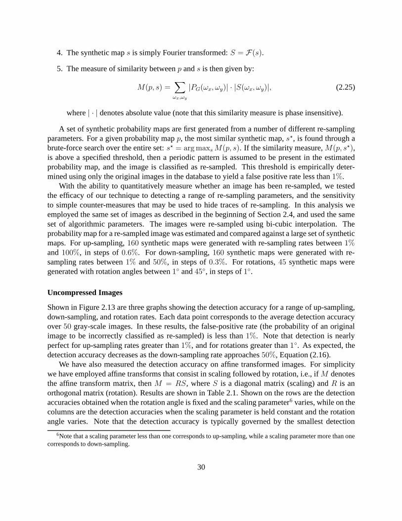
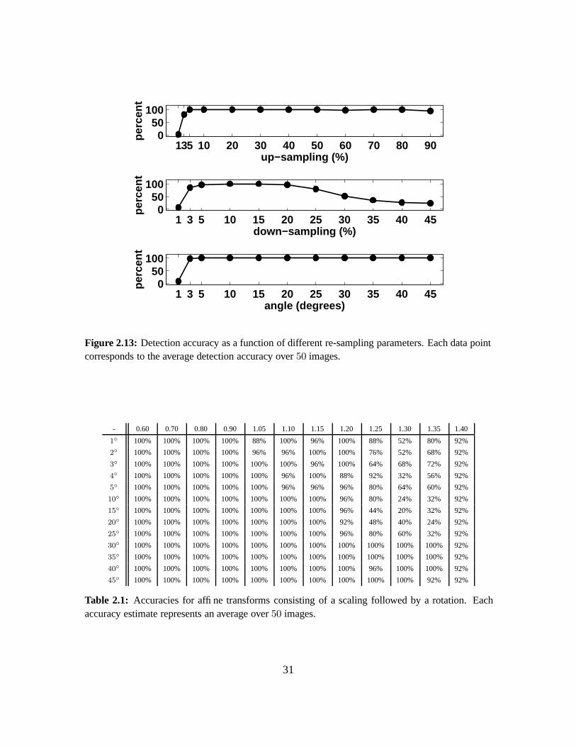
Shown in Figure 2.13 are three graphs showing the detection accuracy for a range of up-sampling,down-sampling, and rotation rates. Each data point corresponds to the average detection accuracyover 50 gray-scale images. In these results, the false-positive rate (the probability of an originalimage to be incorrectly classified as re-sampled) is less than 1%. Note that detection is nearlyperfect for up-sampling rates greater than 1%, and for rotations greater than 1◦. As expected, thedetection accuracy decreases as the down-sampling rate approaches 50%, Equation (2.16).

We have also measured the detection accuracy on affine transformed images. For simplicitywe have employed affine transforms that consist in scaling followed by rotation, i.e., if M denotesthe affine transform matrix, then M = RS, where S is a diagonal matrix (scaling) and R is anorthogonal matrix (rotation). Results are shown in Table 2.1. Shown on the rows are the detectionaccuracies obtained when the rotation angle is fixed and the scaling parameter6 varies, while on thecolumns are the detection accuracies when the scaling parameter is held constant and the rotationangle varies. Note that the detection accuracy is typically governed by the smallest detection

6Note that a scaling parameter less than one corresponds to up-sampling, while a scaling parameter more than onecorresponds to down-sampling.

30

135 10 20 30 40 50 60 70 80 900

50100

up−sampling (%)

perc

ent

1 3 5 10 15 20 25 30 35 40 450

50100

down−sampling (%)

perc

ent

1 3 5 10 15 20 25 30 35 40 450

50100

angle (degrees)

per

cen

t

Figure 2.13: Detection accuracy as a function of different re-sampling parameters. Each data pointcorresponds to the average detection accuracy over 50 images.

- 0.60 0.70 0.80 0.90 1.05 1.10 1.15 1.20 1.25 1.30 1.35 1.40

1◦ 100% 100% 100% 100% 88% 100% 96% 100% 88% 52% 80% 92%

2◦ 100% 100% 100% 100% 96% 96% 100% 100% 76% 52% 68% 92%

3◦ 100% 100% 100% 100% 100% 100% 96% 100% 64% 68% 72% 92%

4◦ 100% 100% 100% 100% 100% 96% 100% 88% 92% 32% 56% 92%

5◦ 100% 100% 100% 100% 100% 96% 96% 96% 80% 64% 60% 92%

10◦ 100% 100% 100% 100% 100% 100% 100% 96% 80% 24% 32% 92%

15◦ 100% 100% 100% 100% 100% 100% 100% 96% 44% 20% 32% 92%

20◦ 100% 100% 100% 100% 100% 100% 100% 92% 48% 40% 24% 92%

25◦ 100% 100% 100% 100% 100% 100% 100% 96% 80% 60% 32% 92%

30◦ 100% 100% 100% 100% 100% 100% 100% 100% 100% 100% 100% 92%

35◦ 100% 100% 100% 100% 100% 100% 100% 100% 100% 100% 100% 92%

40◦ 100% 100% 100% 100% 100% 100% 100% 100% 96% 100% 100% 92%

45◦ 100% 100% 100% 100% 100% 100% 100% 100% 100% 100% 92% 92%

Table 2.1: Accuracies for affine transforms consisting of a scaling followed by a rotation. Eachaccuracy estimate represents an average over 50 images.

31

accuracy of the multiple re-samplings, i.e. for small rotation angles and for large down-samplingfactors the detection accuracy decreases.

The generalization of our algorithm to color images is fairly straightforward — each colorchannel is independently subjected to the same analysis as that employed for gray-scale images.Shown in Figures 2.14-2.15 are the detection accuracies for each color channel treated as an in-dependent gray-scale image, as well as the accuracy when at least one channel is detected as re-sampled. These accuracies were estimated over the same ranges of up-sampling, down-sampling,and rotation rates as those used in the gray-scale experiments. Each data point corresponds to anaverage detection accuracy over 50 color images, with a false-positive rate of less than 1%. Notethat these results are very similar to those obtained for gray-scale images, with a slight improve-ment for larger down-sampling rates.

Robustness to Simple Counter-attacks

In a forensic context, the robustness of our detection algorithm is of particular interest. To thisend, we have tested our method’s capability to resist two simple counter-attacks: additive whiteGaussian noise and non-linear gamma correction. Specifically, after re-sampling an image we ei-ther added a controlled amount of white Gaussian noise, or applied gamma correction with varyinggamma values.

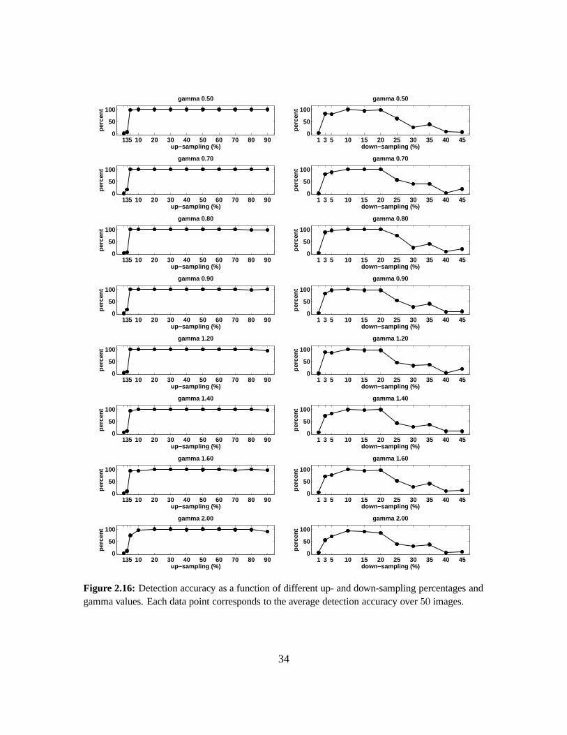
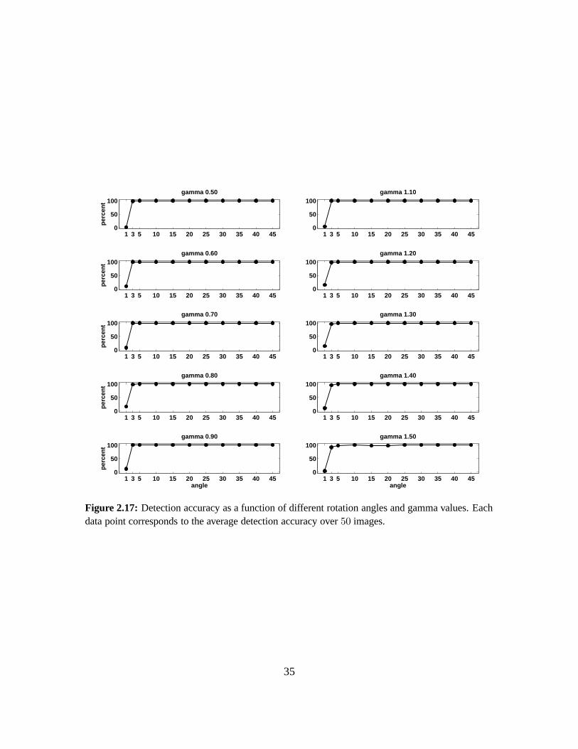
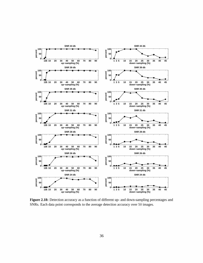
Shown in Figures 2.16-2.17 are the detection accuracies for a range of up-sampling, down-sampling, and rotation rates, and for a range of reasonable gamma values. Note that the detectionaccuracy is practically unaffected by non-linear gamma correction for a large range of gammavalues. Shown in Figures 2.18-2.19 are the detection accuracies for the same range of up-sampling,down-sampling, and rotation rates, and for a range of reasonably chosen signal-to-noise ratios(SNR). Note that the performance for up-sampling and rotation remains good even for low SNRs,e.g., 26 db, except for lower up-sampling percentages (1% − 5%) and smaller rotation angles(1◦ − 5◦). In the case of down-sampling the drop in the detection accuracy is more pronounced,and can be particularly noticed between 35 db and 31 db. Each data point corresponds to theaverage detection accuracy over 50 images, with a false-positive rate of less than 1%, in both thewhite noise and gamma correction experiments.

It may seem surprising that, although the additive noise or non-linear luminance transformsmay destroy or alter the correlations introduced by re-sampling, our algorithm can still detectthese correlations. The reason for this robustness is that the EM algorithm employs a model ofcorrelations that are already corrupted by noise, Equation (2.10). As a result, the accuracy ofre-sampling detection is largely insensitive to small perturbations, and drops gracefully when theamount of perturbation increases.

Robustness to JPEG, JPEG2000, and GIF

We have also tested our algorithm against images compressed with lossy compression algorithms:JPEG [1], GIF, and JPEG2000 [3]. Specifically, gray-scale (for JPEG and JPEG 2000) and color(for GIF) images were subjected to re-sampling with a range of parameters, then compressed and

32

135 10 20 30 40 50 60 70 80 900

50

100

up−sampling (%)

perc

ent

red channel

1 3 5 10 15 20 25 30 35 40 450

50

100

down−sampling (%)

perc

ent

red channel

135 10 20 30 40 50 60 70 80 900

50

100

up−sampling (%)

perc

ent

green channel

1 3 5 10 15 20 25 30 35 40 450

50

100

down−sampling (%)

perc

ent

green channel

135 10 20 30 40 50 60 70 80 900

50

100

up−sampling (%)

perc

ent

blue channel

1 3 5 10 15 20 25 30 35 40 450

50

100

down−sampling (%)

perc

ent

blue channel

135 10 20 30 40 50 60 70 80 900

50

100

up−sampling (%)

perc

ent

at least one channel

1 3 5 10 15 20 25 30 35 40 450

50

100

down−sampling (%)

perc

ent


Figure 2.14: Detection accuracy as a function of different up- and down-sampling percentages fordifferent channels of color images. Each data point corresponds to the average detection accuracyover 50 images.

1 3 5 10 15 20 25 30 35 40 450

50

100

angle (degrees)

per

cen

t

red channel

1 3 5 10 15 20 25 30 35 40 450

50

100

angle (degrees)

per

cen

t

blue channel

1 3 5 10 15 20 25 30 35 40 450

50

100

angle (degrees)

per

cen

t

green channel

1 3 5 10 15 20 25 30 35 40 450

50

100

angle (degrees)

per

cen

t


Figure 2.15: Detection accuracy as a function of different rotation angles for different channels ofcolor images. Each data point corresponds to the average detection accuracy over 50 images.

33

135 10 20 30 40 50 60 70 80 900

50

100

up−sampling (%)

perc

ent

gamma 0.50

1 3 5 10 15 20 25 30 35 40 450

50

100

down−sampling (%)

perc

ent

gamma 0.50

135 10 20 30 40 50 60 70 80 900

50

100

up−sampling (%)

perc

ent

gamma 0.70

1 3 5 10 15 20 25 30 35 40 450

50

100

down−sampling (%)

perc

ent

gamma 0.70

135 10 20 30 40 50 60 70 80 900

50

100

up−sampling (%)

perc

ent

gamma 0.80

1 3 5 10 15 20 25 30 35 40 450

50

100

down−sampling (%)

perc

ent

gamma 0.80

135 10 20 30 40 50 60 70 80 900

50

100

up−sampling (%)

perc

ent

gamma 0.90

1 3 5 10 15 20 25 30 35 40 450

50

100

down−sampling (%)

perc

ent

gamma 0.90

135 10 20 30 40 50 60 70 80 900

50

100

up−sampling (%)

perc

ent

gamma 1.20

1 3 5 10 15 20 25 30 35 40 450

50

100

down−sampling (%)

perc

ent

gamma 1.20

135 10 20 30 40 50 60 70 80 900

50

100

up−sampling (%)

perc

ent

gamma 1.40

1 3 5 10 15 20 25 30 35 40 450

50

100

down−sampling (%)

perc

ent

gamma 1.40

135 10 20 30 40 50 60 70 80 900

50

100

up−sampling (%)

perc

ent

gamma 1.60

1 3 5 10 15 20 25 30 35 40 450

50

100

down−sampling (%)

perc

ent

gamma 1.60

135 10 20 30 40 50 60 70 80 900

50

100

up−sampling (%)

perc

ent

gamma 2.00

1 3 5 10 15 20 25 30 35 40 450

50

100

down−sampling (%)

perc

ent

gamma 2.00

Figure 2.16: Detection accuracy as a function of different up- and down-sampling percentages andgamma values. Each data point corresponds to the average detection accuracy over 50 images.

34

1 3 5 10 15 20 25 30 35 40 450

50

100

per

cen

t

gamma 0.50

1 3 5 10 15 20 25 30 35 40 450

50

100gamma 1.10

1 3 5 10 15 20 25 30 35 40 450

50

100

per

cen

t

gamma 0.60

1 3 5 10 15 20 25 30 35 40 450

50

100gamma 1.20

1 3 5 10 15 20 25 30 35 40 450

50

100

per

cen

t

gamma 0.70

1 3 5 10 15 20 25 30 35 40 450

50

100gamma 1.30

1 3 5 10 15 20 25 30 35 40 450

50

100

per

cen

t

gamma 0.80

1 3 5 10 15 20 25 30 35 40 450

50

100gamma 1.40

1 3 5 10 15 20 25 30 35 40 450

50

100

angle

per

cen

t

gamma 0.90

1 3 5 10 15 20 25 30 35 40 450

50

100

angle

gamma 1.50

Figure 2.17: Detection accuracy as a function of different rotation angles and gamma values. Eachdata point corresponds to the average detection accuracy over 50 images.

35

135 10 20 30 40 50 60 70 80 900

50

100

up−sampling (%)

perc

ent

SNR 44 db

1 3 5 10 15 20 25 30 35 40 450

50

100

down−sampling (%)

perc

ent

SNR 44 db

135 10 20 30 40 50 60 70 80 900

50

100

up−sampling (%)

perc

ent

SNR 39 db

1 3 5 10 15 20 25 30 35 40 450

50

100

down−sampling (%)

perc

ent

SNR 39 db

135 10 20 30 40 50 60 70 80 900

50

100

up−sampling (%)

perc

ent

SNR 35 db

1 3 5 10 15 20 25 30 35 40 450

50

100

down−sampling (%)pe

rcen

t

SNR 35 db

135 10 20 30 40 50 60 70 80 900

50

100

up−sampling (%)

perc

ent

SNR 31 db

1 3 5 10 15 20 25 30 35 40 450

50

100

down−sampling (%)

perc

ent

SNR 31 db

135 10 20 30 40 50 60 70 80 900

50

100

up−sampling (%)

perc

ent

SNR 28 db

1 3 5 10 15 20 25 30 35 40 450

50

100

down−sampling (%)

perc

ent

SNR 28 db

135 10 20 30 40 50 60 70 80 900

50

100

up−sampling (%)

perc

ent

SNR 26 db

1 3 5 10 15 20 25 30 35 40 450

50

100

down−sampling (%)

perc

ent

SNR 26 db

135 10 20 30 40 50 60 70 80 900

50

100

up−sampling (%)

perc

ent

SNR 24 db

1 3 5 10 15 20 25 30 35 40 450

50

100

down−sampling (%)

perc

ent

SNR 24 db

Figure 2.18: Detection accuracy as a function of different up- and down-sampling percentages andSNRs. Each data point corresponds to the average detection accuracy over 50 images.

36

stored in JPEG, GIF, or JPEG2000 formats. For all the experiments presented below, each datapoint corresponds to an average over 50 images, and the false-positive rate is less than 1%.

Shown in Figures 2.20-2.22 are the detection accuracies for re-sampled gray-scale images thatwere subsequently JPEG compressed with different qualities. These results reveal a weakness ofour method: while the detection accuracies are good at qualities between 97 and 100 (out of 100)there is a precipitous fall at quality 96 for down-samplings and rotations, and at a quality of 90,the detection is nearly at chance for all re-sampling rates. Note also that at an up-sampling rateof 60% and a down-sampling rate of 20% the detection accuracy drops suddenly. This is becausethe periodic JPEG blocking artifacts happen to coincide with the periodic patterns introduced bythese re-sampling parameters — these artifacts do not interfere with the detection of rotations.The reason for the general poor performance of detecting re-sampling in JPEG compressed imagesis two-fold. First, lossy JPEG compression introduces correlated non-white noise into the image(e.g., a compression quality of 90 introduces, on average, 28 db of noise), which significantlyaffects the detection accuracy. Second, and more important, the block artifacts introduced byJPEG introduce very strong periodic patterns that mask and interfere with the periodic patternsintroduced by re-sampling.

Shown in Figures 2.23-2.24 are the detection accuracies for re-sampled color images that weresubsequently converted to 8-bit indexed color format (GIF). This conversion introduces approx-imately 25 db of noise. Note that while not as good as the uncompressed TIFF images, thesedetection rates are slightly superior (for down-sampling in particular) to what would be expectedwith the level of noise (see Figures 2.18-2.19) introduced by GIF compression.

We have also tested our method’s robustness with JPEG2000 [3] compression. We have em-ployed a free, non-official JavaTM implementation of the JPEG2000 baseline codec, JJ2000 [54],freely available to download at

http://jj2000.epfl.ch/jj_download/index.html .

Shown in Figures 2.26-2.25 are the results for gray-scale images that were first re-sampled with arange of parameters, then compressed with different numbers of bits per pixel using the JPEG2000codec. Note that the detection remains robust down to 2 bits per pixel. A significant deteriorationis experienced for compression rates below 1.5 bits per pixel (for down-sampling in particular).Note also that the detection accuracy for higher up-sampling rates is lower when compared toTIFF images. The reason for this decrease in accuracy is that JPEG2000 introduces artifacts in theprobability maps that interfere with periodic high frequency patterns like those produced by up-samplings with higher percentages. These artifacts, however, are not as severe as those introducedby JPEG, hence the improved overall performance.

2.5 Summary

When creating digital forgeries, it is often necessary to scale, rotate, or distort a portion of animage. This process involves re-sampling the original image onto a new lattice. Although thisre-sampling process typically leaves behind no perceptual artifacts, it does introduce periodic cor-relations between neighboring image pixels. We have shown how and when correlation patterns

37

1 3 5 10 15 20 25 30 35 40 450

50

100p

erce

nt

SNR 44 db

1 3 5 10 15 20 25 30 35 40 450

50

100SNR 31 db

1 3 5 10 15 20 25 30 35 40 450

50

100

per

cen

t

SNR 40 db

1 3 5 10 15 20 25 30 35 40 450

50

100SNR 28 db

1 3 5 10 15 20 25 30 35 40 450

50

100

per

cen

t

SNR 36 db

1 3 5 10 15 20 25 30 35 40 450

50

100SNR 26 db

1 3 5 10 15 20 25 30 35 40 450

50

100

angle

per

cen

t

SNR 34 db

1 3 5 10 15 20 25 30 35 40 450

50

100

angle

SNR 24 db

Figure 2.19: Detection accuracy as a function of different rotation angles and SNRs. Each datapoint corresponds to the average detection accuracy over 50 images.

135 10 20 30 40 50 60 70 80 900

50

100

up−sampling (%)

perc

ent

JPEG quality 100

135 10 20 30 40 50 60 70 80 900

50

100

up−sampling (%)

perc

ent

JPEG quality 97

135 10 20 30 40 50 60 70 80 900

50

100

up−sampling (%)

perc

ent

JPEG quality 99

135 10 20 30 40 50 60 70 80 900

50

100

up−sampling (%)

perc

ent

JPEG quality 96

135 10 20 30 40 50 60 70 80 900

50

100

up−sampling (%)

perc

ent

JPEG quality 98

135 10 20 30 40 50 60 70 80 900

50

100

up−sampling (%)

perc

ent

JPEG quality 95

Figure 2.20: Detection accuracy as a function of different up-sampling percentages and JPEG com-pression qualities. Each data point corresponds to the average detection accuracy over 50 images.

38

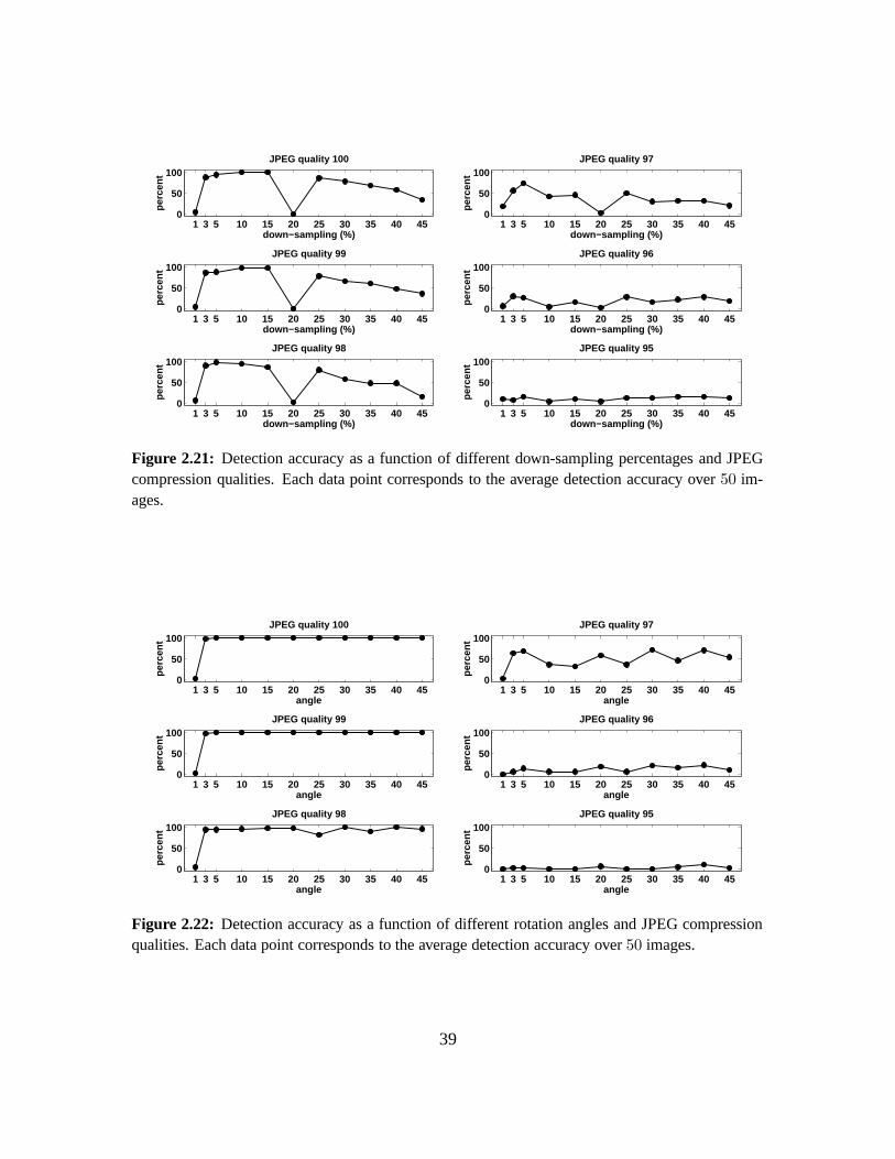
1 3 5 10 15 20 25 30 35 40 450

50

100

down−sampling (%)

perc

ent

JPEG quality 100

1 3 5 10 15 20 25 30 35 40 450

50

100

down−sampling (%)

perc

ent

JPEG quality 97

1 3 5 10 15 20 25 30 35 40 450

50

100

down−sampling (%)

perc

ent

JPEG quality 99

1 3 5 10 15 20 25 30 35 40 450

50

100

down−sampling (%)

perc

ent

JPEG quality 96

1 3 5 10 15 20 25 30 35 40 450

50

100

down−sampling (%)

perc

ent

JPEG quality 98

1 3 5 10 15 20 25 30 35 40 450

50

100

down−sampling (%)

perc

ent

JPEG quality 95

Figure 2.21: Detection accuracy as a function of different down-sampling percentages and JPEGcompression qualities. Each data point corresponds to the average detection accuracy over 50 im-ages.

1 3 5 10 15 20 25 30 35 40 450

50

100

angle

per

cen

t

JPEG quality 100

1 3 5 10 15 20 25 30 35 40 450

50

100

angle

per

cen

t

JPEG quality 97

1 3 5 10 15 20 25 30 35 40 450

50

100

angle

per

cen

t

JPEG quality 99

1 3 5 10 15 20 25 30 35 40 450

50

100

angle

per

cen

t

JPEG quality 96

1 3 5 10 15 20 25 30 35 40 450

50

100

angle

per

cen

t

JPEG quality 98

1 3 5 10 15 20 25 30 35 40 450

50

100

angle

per

cen

t

JPEG quality 95

Figure 2.22: Detection accuracy as a function of different rotation angles and JPEG compressionqualities. Each data point corresponds to the average detection accuracy over 50 images.

39

135 10 20 30 40 50 60 70 80 900

50

100

up−sampling (%)

perc

ent

red channel

1 3 5 10 15 20 25 30 35 40 450

50

100

down−sampling (%)

perc

ent

red channel

135 10 20 30 40 50 60 70 80 900

50

100

up−sampling (%)

perc

ent

green channel

1 3 5 10 15 20 25 30 35 40 450

50

100

down−sampling (%)

perc

ent

green channel

135 10 20 30 40 50 60 70 80 900

50

100

up−sampling (%)

perc

ent

blue channel

1 3 5 10 15 20 25 30 35 40 450

50

100

down−sampling (%)

perc

ent

blue channel

135 10 20 30 40 50 60 70 80 900

50

100

up−sampling (%)

perc

ent


1 3 5 10 15 20 25 30 35 40 450

50

100

down−sampling (%)

perc

ent


Figure 2.23: Detection accuracy as a function of different up- and down-sampling percentages fordifferent channels of color images stored in GIF format. Each data point corresponds to the averagedetection accuracy over 50 images.

1 3 5 10 15 20 25 30 35 40 450

50

100

angle (degrees)

per

cen

t

red channel

1 3 5 10 15 20 25 30 35 40 450

50

100

angle (degrees)

per

cen

t

blue channel

1 3 5 10 15 20 25 30 35 40 450

50

100

angle (degrees)

per

cen

t

green channel

1 3 5 10 15 20 25 30 35 40 450

50

100

angle (degrees)

per

cen

t


Figure 2.24: Detection accuracy as a function of different rotation angles for different channels ofcolor images stored in GIF format. Each data point corresponds to the average detection accuracyover 50 images.

40

1 3 5 10 15 20 25 30 35 40 450

50

100

angle (degrees)

per

cen

t

1.50 bits per pixel

1 3 5 10 15 20 25 30 35 40 450

50

100

angle (degrees)

per

cen

t

1.75 bits per pixel

1 3 5 10 15 20 25 30 35 40 450

50

100

angle (degrees)

per

cen

t

2.00 bits per pixel

1 3 5 10 15 20 25 30 35 40 450

50

100

angle (degrees)

per

cen

t

2.25 bits per pixel

1 3 5 10 15 20 25 30 35 40 450

50

100

angle (degrees)

per

cen

t

2.50 bits per pixel

1 3 5 10 15 20 25 30 35 40 450

50

100

angle (degrees)

per

cen

t

2.75 bits per pixel

1 3 5 10 15 20 25 30 35 40 450

50

100

angle (degrees)

per

cen

t

3.00 bits per pixel

Figure 2.25: Detection accuracy as a function of different rotation angles and JPEG2000 com-pression in bits per pixel. Each data point corresponds to the average detection accuracy over 50

images.

41

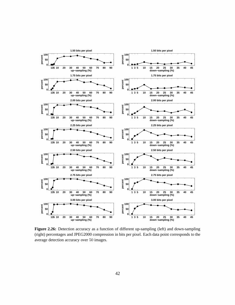
135 10 20 30 40 50 60 70 80 900

50

100

up−sampling (%)

perc

ent

1.50 bits per pixel

1 3 5 10 15 20 25 30 35 40 450

50

100

down−sampling (%)

perc

ent

1.50 bits per pixel

135 10 20 30 40 50 60 70 80 900

50

100

up−sampling (%)

perc

ent

1.75 bits per pixel

1 3 5 10 15 20 25 30 35 40 450

50

100

down−sampling (%)

perc

ent

1.75 bits per pixel

135 10 20 30 40 50 60 70 80 900

50

100

up−sampling (%)

perc

ent

2.00 bits per pixel

1 3 5 10 15 20 25 30 35 40 450

50

100

down−sampling (%)pe

rcen

t

2.00 bits per pixel

135 10 20 30 40 50 60 70 80 900

50

100

up−sampling (%)

perc

ent

2.25 bits per pixel

1 3 5 10 15 20 25 30 35 40 450

50

100

down−sampling (%)

perc

ent

2.25 bits per pixel

135 10 20 30 40 50 60 70 80 900

50

100

up−sampling (%)

perc

ent

2.50 bits per pixel

1 3 5 10 15 20 25 30 35 40 450

50

100

down−sampling (%)

perc

ent

2.50 bits per pixel

135 10 20 30 40 50 60 70 80 900

50

100

up−sampling (%)

perc

ent

2.75 bits per pixel

1 3 5 10 15 20 25 30 35 40 450

50

100

down−sampling (%)

perc

ent

2.75 bits per pixel

135 10 20 30 40 50 60 70 80 900

50

100

up−sampling (%)

perc

ent

3.00 bits per pixel

1 3 5 10 15 20 25 30 35 40 450

50

100

down−sampling (%)

perc

ent

3.00 bits per pixel

Figure 2.26: Detection accuracy as a function of different up-sampling (left) and down-sampling(right) percentages and JPEG2000 compression in bits per pixel. Each data point corresponds to theaverage detection accuracy over 50 images.

42

are introduced, and described a technique to detect them in any portion of an image. We haveshown several detection results on natural test images and credible forgeries, and we have thor-oughly tested our method’s robustness and sensitivity to simple counter-attacks (additive whiteGaussian noise and non-linear luminance transformations) and lossy compression schemes (GIF,JPEG2000, and JPEG). In summary, we have shown that for uncompressed TIFF images, and lossycompressed images with minimal compression we can detect whether an image, or a portion of it,has been re-sampled (scaled, rotated, etc.), as might occur when the image has been tampered with.

43

2.6 Re-sampling Detection Algorithm

/* Initialize */

choose a random ~α0

choose N and σ0

set p0 as 1 over the size of the range of possible values for y(i)

set Y as in Equation (2.15)

set h to be a binomial low-pass filter of size (Nh × Nh)

n = 0

repeat

/* expectation step */

for each sample i

R(i) =∣

∣

∣y(i) −∑N

k=−N αn(k)y(i + k)∣

∣

∣/* residual error */

end

R = R ? h /* spatially average the residual error */

for each sample i

P (i) = 1σn

√2π

e−R2(i)/2σ2n /* conditional probability */

w(i) = P (i)P (i)+p0

/* posterior probability */

end

/* maximization step */

W = 0

for each sample i

W (i, i) = w(i) /* weighting matrix */

end

σn+1 =(

P

i w(i) R2(i)P

i w(i)

)1/2

/* new variance estimate */

~αn+1 = (Y T WY )−1Y T W~y /* new estimate */

n = n + 1

until ( ‖~αn − ~αn−1‖ < ε ) /* stopping condition */

44

Chapter 3

Color Filter Array Interpolated Images

Most digital cameras capture color images using a single sensor in conjunction with an array ofcolor filters. As a result, only one third of the samples in a color image are captured by thecamera, the other two thirds being interpolated. This interpolation introduces specific correlationsbetween the samples of a color image. When creating digital forgeries these correlations are likelyto be destroyed or altered. We describe the form of these correlations, and propose a method thatquantifies and estimates them in any portion of an image. We show the general effectiveness ofthis technique in detecting tampered images, and analyze its sensitivity and robustness to simplecounter-attacks.

3.1 Color Filter Array Interpolation Algorithms

A digital color image consists of three channels containing samples from different bands of thecolor spectrum (e.g., red, green, and blue). Most digital cameras, however, are equipped witha single charge-coupled device (CCD) or complementary metal oxide semiconductor (CMOS)sensor, and capture color images using a color filter array (CFA). The most frequently used colorfilter array (CFA), the Bayer array [4], employs three color filters: red, green, and blue. The red andblue pixels are sampled on rectilinear lattices, while the green pixels are sampled on a quincunxlattice, Figure 3.1. Since only a single color sample is recorded at each pixel location, the other twocolor samples must be estimated from the neighboring samples in order to obtain a three-channelcolor image. Let S(x, y) denote the CFA image in Figure 3.1, and R(x, y), G(x, y), B(x, y) denotethe red, green, and blue channels constructed from S(x, y) by inserting zeros at the locations ofmissing color samples:

R(x, y) =

{

S(x, y) if S(x, y) = rx,y

0 otherwise(3.1)

G(x, y) =

{

S(x, y) if S(x, y) = gx,y

0 otherwise(3.2)

45

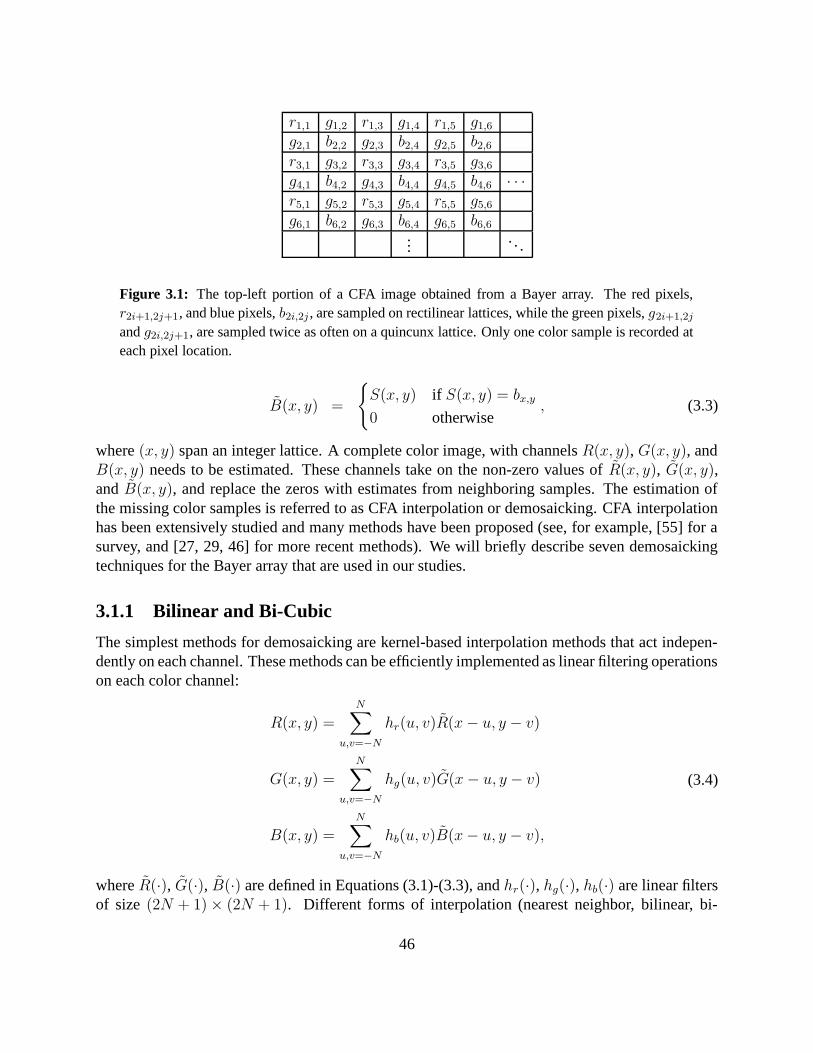
r1,1 g1,2 r1,3 g1,4 r1,5 g1,6

g2,1 b2,2 g2,3 b2,4 g2,5 b2,6

r3,1 g3,2 r3,3 g3,4 r3,5 g3,6

g4,1 b4,2 g4,3 b4,4 g4,5 b4,6 · · ·r5,1 g5,2 r5,3 g5,4 r5,5 g5,6

g6,1 b6,2 g6,3 b6,4 g6,5 b6,6

.... . .

Figure 3.1: The top-left portion of a CFA image obtained from a Bayer array. The red pixels,r2i+1,2j+1, and blue pixels, b2i,2j , are sampled on rectilinear lattices, while the green pixels, g2i+1,2j

and g2i,2j+1, are sampled twice as often on a quincunx lattice. Only one color sample is recorded ateach pixel location.

B(x, y) =

{

S(x, y) if S(x, y) = bx,y

0 otherwise, (3.3)

where (x, y) span an integer lattice. A complete color image, with channels R(x, y), G(x, y), andB(x, y) needs to be estimated. These channels take on the non-zero values of R(x, y), G(x, y),and B(x, y), and replace the zeros with estimates from neighboring samples. The estimation ofthe missing color samples is referred to as CFA interpolation or demosaicking. CFA interpolationhas been extensively studied and many methods have been proposed (see, for example, [55] for asurvey, and [27, 29, 46] for more recent methods). We will briefly describe seven demosaickingtechniques for the Bayer array that are used in our studies.

3.1.1 Bilinear and Bi-Cubic

The simplest methods for demosaicking are kernel-based interpolation methods that act indepen-dently on each channel. These methods can be efficiently implemented as linear filtering operationson each color channel:

R(x, y) =

N∑

u,v=−N

hr(u, v)R(x − u, y − v)

G(x, y) =

N∑

u,v=−N

hg(u, v)G(x − u, y − v)

B(x, y) =N∑

u,v=−N

hb(u, v)B(x − u, y − v),

(3.4)

where R(·), G(·), B(·) are defined in Equations (3.1)-(3.3), and hr(·), hg(·), hb(·) are linear filtersof size (2N + 1) × (2N + 1). Different forms of interpolation (nearest neighbor, bilinear, bi-

46

cubic [32], etc.) differ in the form of the interpolation filter used. For example, in the case of aBayer array, the bilinear and bi-cubic filters for the red and blue channels are separable, with the1-D filters given by:

hl =[

1/2 1 1/2]

hc =[

−1/16 0 9/16 1 9/16 0 −1/16]

. (3.5)

and the 2-D filters given by hTl hl and hT

c hc. The bilinear and bi-cubic filters for the greenchannel, however, are no longer separable and take the form:

hl =1

4

0 1 01 4 10 1 0

hc =1

256

0 0 0 1 0 0 00 0 −9 0 −9 0 00 −9 0 81 0 −9 01 0 81 256 81 0 10 −9 0 81 0 −9 00 0 −9 0 −9 0 00 0 0 1 0 0 0

. (3.6)

Using bilinear interpolation, for example, the color samples at pixel locations (3, 3), (3, 4), and(4, 4), Figure 3.1, are given by:

R(3, 3) = r3,3 G(3, 3) =g2,3 + g3,2 + g3,4 + g4,3

4B(3, 3) =

b2,2 + b2,4 + b4,2 + b4,4

4

G(3, 4) = g3,4 B(3, 4) =b2,4 + b4,4

2R(3, 4) =

r3,3 + r3,5

2

B(4, 4) = b4,4 R(4, 4) =r3,3 + r3,5 + r5,3 + r5,5

4G(4, 4) =

g3,4 + g4,3 + g4,5 + g5,4

4.

3.1.2 Smooth Hue Transition

Smooth hue transition CFA interpolation [10] is based on the assumption that color hue variessmoothly in natural images, and can be assumed to be constant in a small neighborhood. Hue isdefined here as the ratio between a chrominance component (red or blue) and the luminance com-ponent (green). The algorithm interpolates the green channel G(·), Equation (3.2), using bilinearinterpolation, Section 3.1.1, to yield G(·). To estimate the missing red samples, the ratio R(·)/G(·)is bilinearly interpolated, then point-wise multiplied by G(·). For example, the missing red valuesat locations (3, 4), (4, 3), and (4, 4), Figure 3.1, are given by:

R(3, 4) = G(3, 4) · 1

2

(

r3,3

G(3, 3)+

r3,5

G(3, 5)

)

R(4, 3) = G(4, 3) · 1

2

(

r3,3

G(3, 3)+

r5,3

G(5, 3)

)

R(4, 4) = G(4, 4) · 1

4

(

r3,3

G(3, 3)+

r3,5

G(3, 5)+

r5,3

G(5, 3)+

r5,5

G(5, 5)

)

.

(3.7)

The missing blue samples are estimated in a similar manner as the red samples.

47

3.1.3 Median Filter

Median filter based CFA interpolation [20] is a two-step process. First the R(·), G(·), B(·) chan-nels, Equations (3.1)-(3.3), are each interpolated using bilinear interpolation, Section 3.1.1. Next,the pairwise differences of the interpolated channels (i.e., red minus green, red minus blue, andgreen minus blue) are median filtered1. Let Mrg(·), Mgb(·), and Mrb(·) denote the median filtereddifferences. At each pixel location, the missing color samples are estimated as the sum or differ-ence between the color samples from the CFA image, Figure 3.1, and the corresponding medianfiltered differences. For example, the missing samples at locations (3, 3), (3, 4), and (4, 4) areestimated as follows:

G(3, 3) = r3,3 − Mrg(3, 3) B(3, 3) = r3,3 − Mrb(3, 3)

R(3, 4) = g3,4 + Mrg(3, 4) B(3, 4) = g3,4 − Mgb(3, 4)

R(4, 4) = b4,4 + Mrb(4, 4) G(4, 4) = b4,4 + Mgb(4, 4).

(3.8)

3.1.4 Gradient-Based

Gradient-based CFA interpolation [36] is a multi-step method that preserves edge information bytrying to prevent interpolation across edges. The green channel, G(·), is first estimated using anadaptive interpolation technique. For example, in order to estimate the green values at location(3, 3) and (4, 4), Figure 3.1, derivative estimators along the horizontal and vertical directions arefirst computed:

H3,3 = |(r3,1 + r3,5)/2 − r3,3| V3,3 = |(r1,3 + r5,3)/2 − r3,3|H4,4 = |(b4,2 + b4,6)/2 − b4,4| V4,4 = |(b2,4 + b6,4)/2 − b4,4| .

(3.9)

These estimators are referred to as classifiers. The estimated green values are then given by:

G(3, 3) =

(g3,2 + g3,4)/2 H3,3 < V3,3

(g2,3 + g4,3)/2 H3,3 > V3,3

(g2,3 + g3,2 + g3,4 + g4,3)/4 H3,3 = V3,3

G(4, 4) =

(g4,3 + g4,5)/2 H4,4 < V4,4

(g3,4 + g5,4)/2 H4,4 > V4,4

(g3,4 + g4,3 + g4,5 + g5,4)/4 H4,4 = V4,4.

(3.10)

The missing red samples are estimated by taking the difference image between the R(·) andG(·) channels, bilinearly interpolating this difference, then adding back G(·). For example, themissing red samples at (3, 4), (4, 3), and (4, 4), Figure 3.1, are given by:

R(3, 4) =1

2

[

(

r3,3 − G(3, 3))

+(

r3,5 − G(3, 5))

]

+ G(3, 4) (3.11)

1The choice of the median filter size is important for the perceptual quality of CFA interpolated images.

48

R(4, 3) =1

2

[

(

r3,3 − G(3, 3))

+(

r5,3 − G(5, 3))

]

+ G(4, 3) (3.12)

R(4, 4) =1

4

[

(

r3,3 − G(3, 3))

+(

r3,5 − G(3, 5))

+(

r5,3 − G(5, 3))

+ (3.13)(

r5,5 − G(5, 5))

]

+ G(4, 4).

The missing blue samples are estimated in a similar manner as the red samples.

3.1.5 Adaptive Color Plane

Adaptive color plane CFA interpolation [28] is a modification of the gradient-based interpolationmethod that includes second-order derivative estimates. The green channel, G(·), is first estimatedusing adaptive interpolation. For example, in order to estimate the green values at (3, 3) and(4, 4), Figure 3.1, horizontal and vertical classifiers are computed as the sum between first-orderderivative estimates from the luminance (green) channel, and second-order derivative estimatesfrom the chrominance (red and blue) channels:

H3,3 = |g3,2 − g3,4| + |−r3,1 + 2r3,3 − r3,5|V3,3 = |g2,3 − g4,3| + |−r1,3 + 2r3,3 − r5,3|H4,4 = |g4,3 − g4,5| + |−b4,2 + 2b4,4 − b4,6|V4,4 = |g3,4 − g5,4| + |−b2,4 + 2b4,4 − b6,4| .

(3.14)

Using these classifiers, the estimated green values are given by:

G(3, 3) =

(g3,2 + g3,4)/2 + (−r3,1 + 2r3,3 − r3,5)/4 H3,3 < V3,3

(g2,3 + g4,3)/2 + (−r1,3 + 2r3,3 − r5,3)/4 H3,3 > V3,3

(g2,3 + g3,2 + g3,4 + g4,3)/4 +

(−r1,3 − r3,1 + 4r3,3 − r3,5 − r5,3)/8 H3,3 = V3,3

G(4, 4) =

(g4,3 + g4,5)/2 + (−b4,2 + 2b4,4 − b4,6)/4 H4,4 < V4,4

(g3,4 + g5,4)/2 + (−b2,4 + 2b4,4 − b6,4)/4 H4,4 > V4,4

(g3,4 + g4,3 + g4,5 + g5,4)/4 +

(−b2,4 − b4,2 + 4b4,4 − b4,6 − b6,4)/8 H4,4 = V4,4.

(3.15)

The estimation of the missing chrominance samples depends on their location in the CFA. Atlocations where the nearest chrominance samples are in the same row or column, a non-adaptiveprocedure with second-order correction terms is employed. For example, red and blue samples at(3, 4) and (4, 3) are given by:

R(3, 4) =r3,3 + r3,5

2+

−G(3, 3) + 2G(3, 4) − G(3, 5)

2(3.16)

B(3, 4) =b2,4 + b4,4

2+

−G(2, 4) + 2G(3, 4) − G(4, 4)

2(3.17)

49

R(4, 3) =r3,3 + r5,3

2+

−G(3, 3) + 2G(4, 3) − G(5, 3)

2(3.18)

B(4, 3) =b4,2 + b4,4

2+

−G(4, 2) + 2G(4, 3) − G(4, 4)

2. (3.19)

At locations where the nearest chrominance neighbors are diagonally located, an adaptive proce-dure is employed. For example, in order to estimate the missing chrominance samples at (3, 3)and (4, 4), classifiers based on derivative estimates along the first and second diagonals are firstestimated:

D13,3 = |b2,2 − b4,4| + |−G(2, 2) + 2G(3, 3) − G(4, 4)|

D23,3 = |b2,4 − b4,2| + |−G(2, 4) + 2G(3, 3) − G(4, 2)|

D14,4 = |r3,3 − r5,5| + |−G(3, 3) + 2G(4, 4) − G(5, 5)|

D24,4 = |r3,5 − r5,3| + |−G(3, 5) + 2G(4, 4) − G(5, 3)| ,

(3.20)

then using these classifiers, the missing red and blue values are given by:

B(3, 3) =

(b2,4 + b4,2)/2 + (−G(2, 4) + 2G(3, 3) − G(4, 2))/2 D13,3 > D2

3,3

(b2,2 + b4,4)/2 + (−G(2, 2) + 2G(3, 3) − G(4, 4))/2 D13,3 < D2

3,3

(b2,2 + b2,4 + b4,2 + b4,4)/4 +

(−G(2, 2) − G(2, 4) + 4G(3, 3) − G(4, 2) − G(4, 4))/4 D13,3 = D2

3,3

R(4, 4) =

(r3,5 + r5,3)/2 + (−G(3, 5) + 2G(4, 4) − G(5, 3))/2 D14,4 > D2

4,4

(r3,3 + r5,5)/2 + (−G(3, 3) + 2G(4, 4) − G(5, 5))/2 D14,4 < D2

4,4

(r3,3 + r3,5 + r5,3 + r5,5)/4 +

(−G(3, 3) − G(3, 5) + 4G(4, 4) − G(5, 3) − G(5, 5))/4 D14,4 = D2

4,4.

3.1.6 Threshold-Based Variable Number of Gradients

Threshold-based variable number of gradients CFA interpolation [9] is a more complex demo-saicking method. At each pixel location, eight gradient estimates are first computed using samplesfrom a 5 × 5 neighborhood of the CFA image. These estimates are computed slightly differentlydepending on the color sample at the pixel under consideration: chrominance (red and blue) orluminance (green). For example, the eight gradient estimates at location (3, 3), Figure 3.1, aregiven by:

N3,3 = |g2,3 − g4,3| + |r1,3 − r3,3|+|b2,2 − b4,2|

2+

|b2,4 − b4,4|2

+|g1,2 − g3,2|

2+

|g1,4 − g3,4|2

(3.21)

E3,3 = |g3,2 − g3,4| + |r3,3 − r3,5|+|b2,2 − b2,4|

2+

|b4,2 − b4,4|2

+|g2,3 − g2,5|

2+

|g4,3 − g4,5|2

(3.22)

50

S3,3 = |g2,3 − g4,3| + |r3,3 − r5,3|+|b2,2 − b4,2|

2+

|b2,4 − b4,4|2

+|g3,2 − g5,2|

2+

|g3,4 − g5,4|2

(3.23)

W3,3 = |g3,2 − g3,4| + |r3,1 − r3,3|+|b2,2 − b2,4|

2+

|b4,2 − b4,4|2

+|g2,1 − g2,3|

2+

|g4,1 − g4,3|2

(3.24)

NE3,3 = |b2,4 − b4,2| + |r1,5 − r3,3|+|g2,3 − g3,2|

2+

|g3,4 − g4,3|2

+|g1,4 − g2,3|

2+

|g2,5 − g3,4|2

(3.25)

SE3,3 = |b2,2 − b4,4| + |r3,3 − r5,5|+|g2,3 − g3,4|

2+

|g3,2 − g4,3|2

+|g3,4 − g4,5|

2+

|g4,3 − g5,4|2

(3.26)

NW3,3 = |b2,2 − b4,4| + |r1,1 − r3,3|+|g1,2 − g2,3|

2+

|g2,1 − g3,2|2

+|g2,3 − g3,4|

2+

|g3,2 − g4,3|2

(3.27)

SW3,3 = |b2,4 − b4,2| + |r5,1 − r3,3|+|g2,3 − g3,2|

2+

|g3,4 − g4,3|2

+|g3,2 − g4,1|

2+

|g4,3 − g5,2|2

, (3.28)

and the gradients at location (3, 4), Figure 3.1, are given by:

N3,4 = |b2,4 − b4,4| + |g1,4 − g3,4|+|g2,3 − g4,3|

2+

|g2,5 − g4,5|2

+|r1,3 − r3,3|

2+

|r1,5 − r3,5|2

(3.29)

E3,4 = |r3,3 − r3,5| + |g3,4 − g3,6|+|g2,3 − g2,5|

2+

|g4,3 − g4,5|2

+|b2,4 − b2,6|

2+

|b4,4 − b4,6|2

(3.30)

S3,4 = |b2,4 − b4,4| + |g3,4 − g5,4|+|g2,3 − g4,3|

2+

|g2,5 − g4,5|2

+|r3,3 − r5,3|

2+

|r3,5 − r5,5|2

(3.31)

51

W3,4 = |r3,3 − r3,5| + |g3,2 − g3,4|+|g2,3 − g2,5|

2+

|g4,3 − g4,5|2

+|b2,2 − b2,4|

2+

|b4,2 − b4,4|2

(3.32)

NE3,4 = |g2,5 − g4,3| + |g1,6 − g3,4| + |r1,5 − r3,3| + |b2,6 − b4,4| (3.33)

SE3,4 = |g2,3 − g4,5| + |g3,4 − g5,6| + |b2,4 − b4,6| + |r3,3 − r5,5| (3.34)

NW3,4 = |g2,3 − g4,5| + |g1,2 − g3,4| + |b2,2 − b4,4| + |r1,3 − r3,5| (3.35)

SW3,4 = |g2,5 − g4,3| + |g3,4 − g5,2| + |b2,4 − b4,2| + |r3,5 − r5,3| . (3.36)

Let Gx,y denote the set of gradient estimates at (x, y):

Gx,y = {Nx,y, Sx,y, Ex,y, Wx,y, NEx,y, NWx,y, SEx,y, SWx,y}. (3.37)

Eight average red, green, and blue values, one for each gradient direction, are then computedat each pixel location. At location (3, 3), for example, the average values corresponding to thedifferent gradient regions are given by:

RN3,3 = (r1,3 + r3,3)/2 GN

3,3 = g2,3 BN3,3 = (b2,2 + b2,4)/2

RE3,3 = (r3,3 + r3,5)/2 GE

3,3 = g3,4 BE3,3 = (b2,4 + b4,4)/2

RS3,3 = (r3,3 + r5,3)/2 GS

3,3 = g4,3 BS3,3 = (b4,2 + b4,4)/2

RW3,3 = (r3,1 + r3,3)/2 GW

3,3 = g3,2 BW3,3 = (b2,2 + b4,2)/2

RNE3,3 = (r1,5 + r3,3)/2 GNE

3,3 = (g1,4 + g2,3 + g2,5 + g3,4)/4 BNE3,3 = b2,4

RSE3,3 = (r3,3 + r5,5)/2 GSE

3,3 = (g3,4 + g4,3 + g4,5 + g5,4)/4 BSE3,3 = b4,4

RNW3,3 = (r1,1 + r3,3)/2 GNW

3,3 = (g1,2 + g2,1 + g2,3 + g3,2)/4 BNW3,3 = b2,2

RSW3,3 = (r3,3 + r5,1)/2 GSW

3,3 = (g3,2 + g4,1 + g4,3 + g5,2)/4 BSW3,3 = b4,2

From Gx,y, Equation (3.37), a threshold Tx,y is computed as:

Tx,y = k1 minGx,y + k2(maxGx,y − minGx,y), (3.38)

where the values of k1, k2 are empirically chosen as 1.5 and 0.5, respectively. Next the previouslycomputed color averages from regions whose gradient estimate is less than the threshold, are av-eraged to yield Ravg

x,y , Gavgx,y , and Bavg

x,y . For example, at location (3, 3) if the gradient estimates lessthan T3,3 are S3,3, W3,3, NE3,3, and SW3,3, then:

Ravg3,3 = 1/4 · (RS

3,3 + RW3,3 + RNE

3,3 + RSW3,3 )

Gavg3,3 = 1/4 · (GS

3,3 + GW3,3 + GNE

3,3 + GSW3,3 )

Bavg3,3 = 1/4 · (BS

3,3 + BW3,3 + BNE

3,3 + BSW3,3 ).

(3.39)

The final estimates of the missing color samples at location (3, 3) are then given by:

G(3, 3) = r3,3 + (Gavg3,3 − Ravg

3,3 )

B(3, 3) = r3,3 + (Bavg3,3 − Ravg

3,3 ).(3.40)

The missing color samples at the other pixel locations are estimated in a similar manner.

52

3.2 Detecting CFA Interpolation

At each pixel location of a CFA interpolated color image, a single color sample is captured by thecamera sensor, while the other two color samples are estimated from neighboring samples. As aresult, a subset of samples, within a color channel, are correlated to their neighboring samples.Since the color filters in a CFA are typically arranged in a periodic pattern, these correlationsare periodic. Consider, for example, the red channel, R(x, y), that has been sampled on a Bayerarray, Figure 3.1, then CFA interpolated using bilinear interpolation, Section 3.1.1. In this case,the red samples in the odd rows and even columns are the average of their closest horizontalneighbors, the red samples in the even rows and odd columns are the average of their closestvertical neighbors, and the red samples in the even rows and columns are the average of theirclosest diagonal neighbors:

R(2x + 1, 2y) =R(2x + 1, 2y − 1)

2+

R(2x + 1, 2y + 1)

2

R(2x, 2y + 1) =R(2x − 1, 2y + 1)

2+

R(2x + 1, 2y + 1)

2

R(2x, 2y) =R(2x − 1, 2y − 1)

4+

R(2x − 1, 2y + 1)

4+

R(2x + 1, 2y − 1)

4+

R(2x + 1, 2y + 1)

4.

(3.41)

Note that in this simple case, the estimated samples are perfectly correlated to their neighbors.As such a CFA interpolated image can be detected (in the absence of noise) by noticing, for exam-ple, that every other sample in every other row or column is perfectly correlated to its neighbors.At the same time, the non-interpolated samples are less likely to be correlated in precisely thesame manner. Furthermore, it is likely that tampering will destroy these correlations, or that thesplicing together of two images from different cameras will create inconsistent correlations acrossthe composite image. As such, the presence, or lack, of correlations due to CFA interpolation canbe used to authenticate an image, or expose it as a forgery.

We begin by assuming a simple linear model for the periodic correlations introduced by CFAinterpolation. That is, each interpolated pixel is correlated to a weighted sum of pixels in a smallneighborhood centered about itself. While perhaps overly simplistic when compared to the highlynon-linear nature of most CFA interpolation algorithms, this simple model is both easy to pa-rameterize and can reasonably approximate each of the CFA interpolation algorithms presentedin Section 3.1. Note that most CFA algorithms estimate a missing color sample from neighbor-ing samples in all three color channels. For simplicity, however, we ignore these inter-channelcorrelations and treat each color channel independently.

If the specific form of the correlations are known (i.e., the parameters of the linear model), thenit would be straightforward to determine which samples are correlated to their neighbors. On theother hand, if the samples correlated to their neighbors are known, the specific form of the corre-lations could be easily determined. In practice, of course, neither are known. To simultaneously

53

estimate both we employ the expectation-maximization2 (EM) algorithm [14], as described below.

3.2.1 Expectation-Maximization Algorithm

Let f(·, ·) denote a color channel (red, green, or blue) of a CFA interpolated image. We begin byassuming that each sample in f(·, ·) belongs to one of two models:

M1, if the sample is linearly correlated to its neighbors, i.e., is generated by the linear model:

f(x, y) =

N∑

u,v=−N

αu,vf(x + u, y + v) + n(x, y), (3.42)

where the model parameters are given by ~α = {αu,v| − N ≤ u, v ≤ N} (N is an integer andα0,0 = 0), the linear coefficients (strung out in vector form) that embody the specific formof the correlations, with α0,0 = 0. In the above equation, n(x, y) denote independent, andidentically distributed (i.i.d.) samples drawn from a Gaussian distribution with zero meanand unknown variance σ2.

M2, if the sample is not correlated to its neighbors, i.e., is generated by an outlier process.

The expectation-maximization algorithm (EM) is a two-step iterative algorithm: (1) in the E-stepthe probability of each sample belonging to each model is estimated; and (2) in the M-step thespecific form of the correlations between samples is estimated. More specifically, in the E-step,the probability of each sample of f(x, y) belonging to model M1 is estimated using Bayes’ rule:

Pr{f(x, y) ∈ M1 | f(x, y)} =

Pr{f(x, y) | f(x, y) ∈ M1}Pr{f(x, y) ∈ M1}∑2

i=1 Pr{f(x, y) | f(x, y) ∈ Mi}Pr{f(x, y) ∈ Mi}, (3.43)

where the prior probabilities Pr{f(x, y) ∈ M1} and Pr{f(x, y) ∈ M2} are assumed to be equalto 1/2. The probability of observing a sample f(x, y) knowing it was generated from model M1 isgiven by:

Pr{f(x, y) | f(x, y) ∈ M1} =

1

σ√

2πexp

− 1

2σ2

(

f(x, y) −N∑

u,v=−N

αu,vf(x + u, y + v)

)2

. (3.44)

2A short tutorial on the general EM algorithm, and an example of its application to a mixture models problem arepresented in Appendix A.

54

The variance, σ2, of this Gaussian distribution is estimated in the M-step (see Section 3.5). Auniform distribution is assumed for the probability of observing a sample generated by the outliermodel, M2, i.e., Pr{f(x, y) | f(x, y) ∈ M2} is equal to the inverse of the range of possible valuesof f(x, y). Note that the E-step requires an estimate of the coefficients ~α, which on the first iterationis chosen randomly. In the M-step, a new estimate of ~α is computed using weighted least squares,i.e., minimizing the following quadratic error function:

E(~α) =∑

x,y

w(x, y)

(

f(x, y) −N∑

u,v=−N


)2

, (3.45)

where the weights w(x, y) ≡ Pr{f(x, y) ∈ M1 | f(x, y)}, Equation (3.43). This error functionis minimized by computing the gradient with respect to ~α, setting this gradient equal to zero, andsolving the resulting linear system of equations. Setting equal to zero the partial derivative withrespect to one of the coefficients, αs,t, yields:

∂E

∂αs,t= 0

−2∑

x,y

w(x, y)f(x + s, y + t)

(

f(x, y) −N∑

u,v=−N


)

= 0

∑

x,y

w(x, y)f(x + s, y + t)

N∑

u,v=−N

αu,vf(x + u, y + v) =

∑

x,y

w(x, y)f(x + s, y + t)f(x, y).

(3.46)

Re-ordering the terms on the left-hand side yields:

N∑

u,v=−N

αu,v

(

∑

x,y

w(x, y)f(x + s, y + t)f(x + u, y + v)

)

=

∑

x,y

w(x, y)f(x + s, y + t)f(x, y) . (3.47)

This process is repeated for each component, αs,t, of ~α, to yield a system of linear equations thatcan be solved using standard techniques.

The E-step and the M-step are iteratively executed until a stable estimate of ~α is achieved — seeSection 3.5 for a detailed algorithm. The final ~α has the property that it maximizes the likelihoodof the observed samples3 — see Appendix A for more details on maximum likelihood estimationand EM.

3The EM algorithm is proved to always converge to a stable estimate that is a local maximum of the log-likelihoodof the observed data, [14] and Appendix A.

55

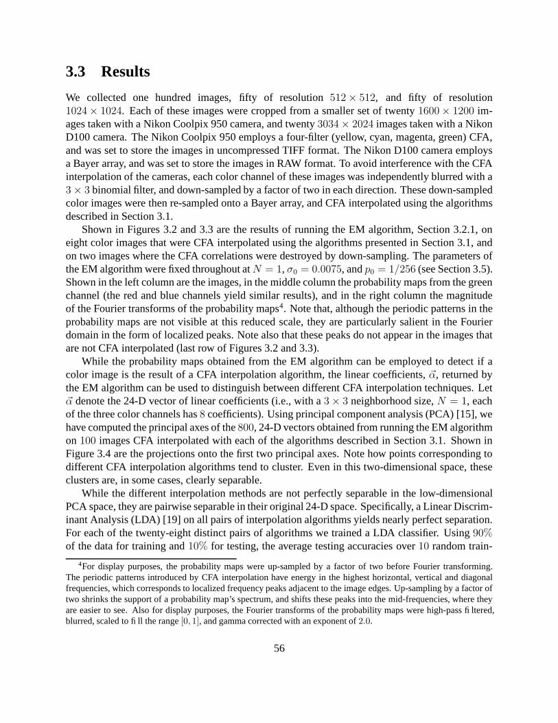
3.3 Results

We collected one hundred images, fifty of resolution 512 × 512, and fifty of resolution1024 × 1024. Each of these images were cropped from a smaller set of twenty 1600 × 1200 im-ages taken with a Nikon Coolpix 950 camera, and twenty 3034 × 2024 images taken with a NikonD100 camera. The Nikon Coolpix 950 employs a four-filter (yellow, cyan, magenta, green) CFA,and was set to store the images in uncompressed TIFF format. The Nikon D100 camera employsa Bayer array, and was set to store the images in RAW format. To avoid interference with the CFAinterpolation of the cameras, each color channel of these images was independently blurred with a3 × 3 binomial filter, and down-sampled by a factor of two in each direction. These down-sampledcolor images were then re-sampled onto a Bayer array, and CFA interpolated using the algorithmsdescribed in Section 3.1.

Shown in Figures 3.2 and 3.3 are the results of running the EM algorithm, Section 3.2.1, oneight color images that were CFA interpolated using the algorithms presented in Section 3.1, andon two images where the CFA correlations were destroyed by down-sampling. The parameters ofthe EM algorithm were fixed throughout at N = 1, σ0 = 0.0075, and p0 = 1/256 (see Section 3.5).Shown in the left column are the images, in the middle column the probability maps from the greenchannel (the red and blue channels yield similar results), and in the right column the magnitudeof the Fourier transforms of the probability maps4. Note that, although the periodic patterns in theprobability maps are not visible at this reduced scale, they are particularly salient in the Fourierdomain in the form of localized peaks. Note also that these peaks do not appear in the images thatare not CFA interpolated (last row of Figures 3.2 and 3.3).

While the probability maps obtained from the EM algorithm can be employed to detect if acolor image is the result of a CFA interpolation algorithm, the linear coefficients, ~α, returned bythe EM algorithm can be used to distinguish between different CFA interpolation techniques. Let~α denote the 24-D vector of linear coefficients (i.e., with a 3 × 3 neighborhood size, N = 1, eachof the three color channels has 8 coefficients). Using principal component analysis (PCA) [15], wehave computed the principal axes of the 800, 24-D vectors obtained from running the EM algorithmon 100 images CFA interpolated with each of the algorithms described in Section 3.1. Shown inFigure 3.4 are the projections onto the first two principal axes. Note how points corresponding todifferent CFA interpolation algorithms tend to cluster. Even in this two-dimensional space, theseclusters are, in some cases, clearly separable.

While the different interpolation methods are not perfectly separable in the low-dimensionalPCA space, they are pairwise separable in their original 24-D space. Specifically, a Linear Discrim-inant Analysis (LDA) [19] on all pairs of interpolation algorithms yields nearly perfect separation.For each of the twenty-eight distinct pairs of algorithms we trained a LDA classifier. Using 90%of the data for training and 10% for testing, the average testing accuracies over 10 random train-

4For display purposes, the probability maps were up-sampled by a factor of two before Fourier transforming.The periodic patterns introduced by CFA interpolation have energy in the highest horizontal, vertical and diagonalfrequencies, which corresponds to localized frequency peaks adjacent to the image edges. Up-sampling by a factor oftwo shrinks the support of a probability map’s spectrum, and shifts these peaks into the mid-frequencies, where theyare easier to see. Also for display purposes, the Fourier transforms of the probability maps were high-pass filtered,blurred, scaled to fill the range [0, 1], and gamma corrected with an exponent of 2.0.

56

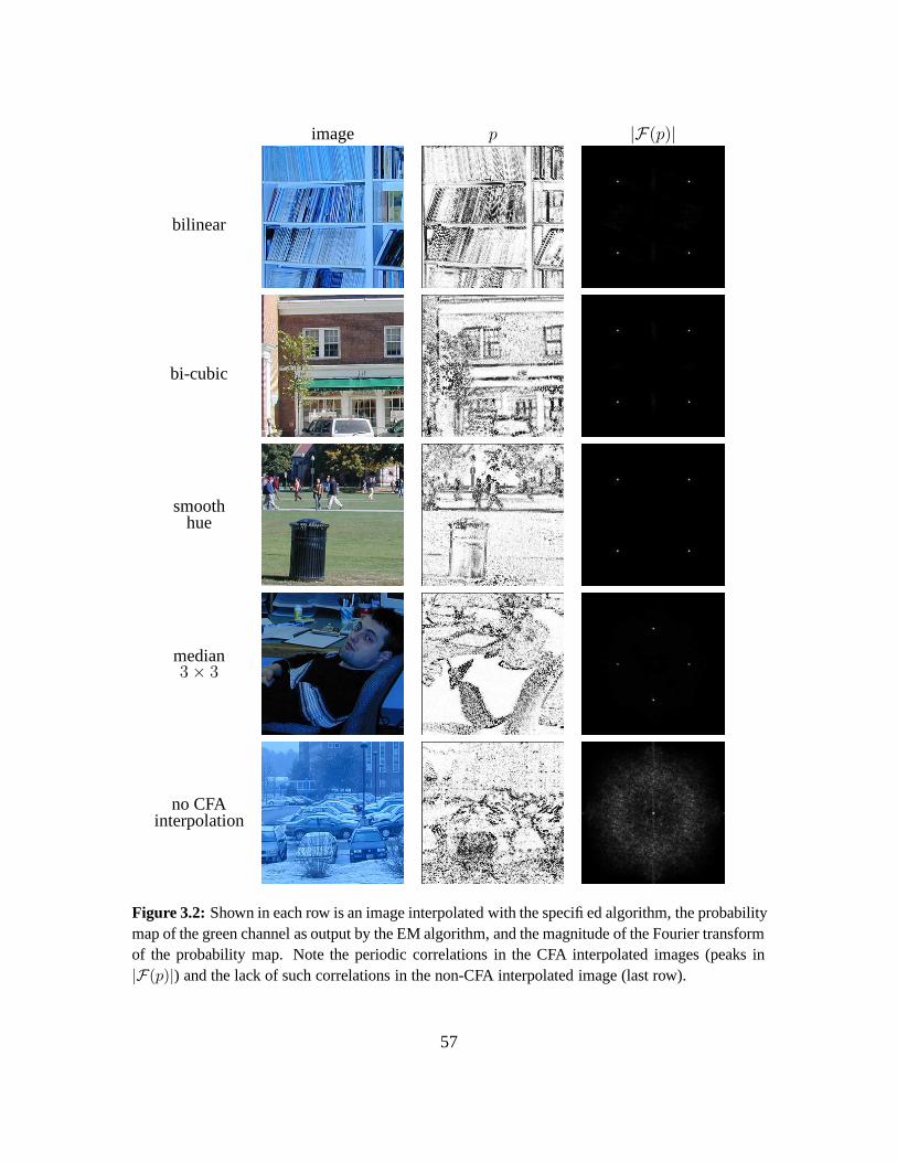
image p |F(p)|

bilinear

bi-cubic

smoothhue

median3 × 3

no CFAinterpolation

Figure 3.2: Shown in each row is an image interpolated with the specified algorithm, the probabilitymap of the green channel as output by the EM algorithm, and the magnitude of the Fourier transformof the probability map. Note the periodic correlations in the CFA interpolated images (peaks in|F(p)|) and the lack of such correlations in the non-CFA interpolated image (last row).

57

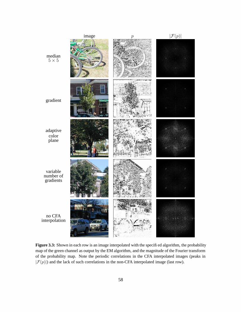
image p |F(p)|

median5 × 5

gradient

adaptivecolorplane

variablenumber ofgradients

no CFAinterpolation

Figure 3.3: Shown in each row is an image interpolated with the specified algorithm, the probabilitymap of the green channel as output by the EM algorithm, and the magnitude of the Fourier transformof the probability map. Note the periodic correlations in the CFA interpolated images (peaks in|F(p)|) and the lack of such correlations in the non-CFA interpolated image (last row).

58

bl bc sh m3 m5 gb acpvng

Figure 3.4: The estimated interpolation coefficients from 100 images CFA interpolated with eightdifferent algorithms are projected onto a 2-D subspace. Even in this reduced space, the algorithmsare, in some cases, clearly separable.

ing/testing splits and over all pairs of algorithms are shown in the Table 3.1. The average overall pairs of algorithms was 97%, and the minimum testing accuracy was 87% and was obtainedwhen separating the 3 × 3 median filter and the variable number of gradients algorithms. Sincedigital cameras typically employ different CFA interpolation algorithms, this result could be usedto determine if an image was not taken with a specific digital camera.

3.3.1 Detecting Localized Tampering

Since it is likely that tampering will destroy the periodic CFA correlations, it may be possibleto detect and localize tampering in any portion of an image. To illustrate this, we begin withthree 1024 × 1024 images, taken with a Nikon D100 digital camera and saved in RAW format,Figure 3.5. To simulate tampering, each color channel of these images (initially interpolated usingthe adaptive color plane technique) was blurred with a 3 × 3 binomial filter and down-sampled bya factor of two in order to destroy the CFA correlations. The 512 × 512 down-sampled imageswere then re-sampled on a Bayer array and CFA interpolated. Next, composite images, 512 × 512pixels in size, were created by splicing, in varying proportions (1/4, 1/2, and 3/4), a non-CFAinterpolated image and the same CFA interpolated image. Shown in Figure 3.6 are the resultsof running EM on these composite images — each row corresponds to a different interpolationalgorithm: from top to bottom, bi-cubic, Section 3.1.1, gradient-based, Section 3.1.4, and variablenumber of gradients, Section 3.1.6. Shown in the top row are the probability maps of the redchannel. Note that these probability maps clearly reveal the presence of two distinct regions. Also

59

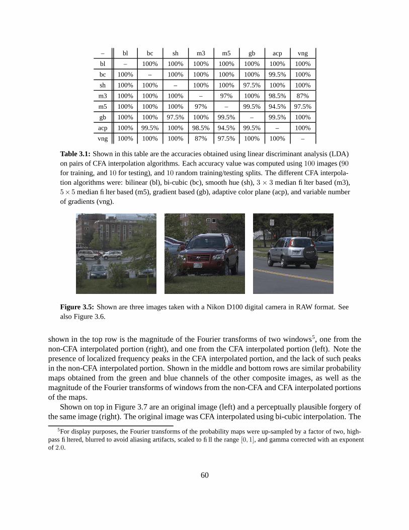
– bl bc sh m3 m5 gb acp vng

bl – 100% 100% 100% 100% 100% 100% 100%

bc 100% – 100% 100% 100% 100% 99.5% 100%

sh 100% 100% – 100% 100% 97.5% 100% 100%

m3 100% 100% 100% – 97% 100% 98.5% 87%

m5 100% 100% 100% 97% – 99.5% 94.5% 97.5%

gb 100% 100% 97.5% 100% 99.5% – 99.5% 100%

acp 100% 99.5% 100% 98.5% 94.5% 99.5% – 100%

vng 100% 100% 100% 87% 97.5% 100% 100% –

Table 3.1: Shown in this table are the accuracies obtained using linear discriminant analysis (LDA)on pairs of CFA interpolation algorithms. Each accuracy value was computed using 100 images (90for training, and 10 for testing), and 10 random training/testing splits. The different CFA interpola-tion algorithms were: bilinear (bl), bi-cubic (bc), smooth hue (sh), 3 × 3 median filter based (m3),5×5 median filter based (m5), gradient based (gb), adaptive color plane (acp), and variable numberof gradients (vng).

Figure 3.5: Shown are three images taken with a Nikon D100 digital camera in RAW format. Seealso Figure 3.6.

shown in the top row is the magnitude of the Fourier transforms of two windows5, one from thenon-CFA interpolated portion (right), and one from the CFA interpolated portion (left). Note thepresence of localized frequency peaks in the CFA interpolated portion, and the lack of such peaksin the non-CFA interpolated portion. Shown in the middle and bottom rows are similar probabilitymaps obtained from the green and blue channels of the other composite images, as well as themagnitude of the Fourier transforms of windows from the non-CFA and CFA interpolated portionsof the maps.

Shown on top in Figure 3.7 are an original image (left) and a perceptually plausible forgery ofthe same image (right). The original image was CFA interpolated using bi-cubic interpolation. The

5For display purposes, the Fourier transforms of the probability maps were up-sampled by a factor of two, high-pass filtered, blurred to avoid aliasing artifacts, scaled to fill the range [0, 1], and gamma corrected with an exponentof 2.0.

60

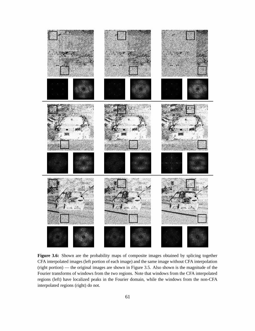
Figure 3.6: Shown are the probability maps of composite images obtained by splicing togetherCFA interpolated images (left portion of each image) and the same image without CFA interpolation(right portion) — the original images are shown in Figure 3.5. Also shown is the magnitude of theFourier transforms of windows from the two regions. Note that windows from the CFA interpolatedregions (left) have localized peaks in the Fourier domain, while the windows from the non-CFAinterpolated regions (right) do not.

61

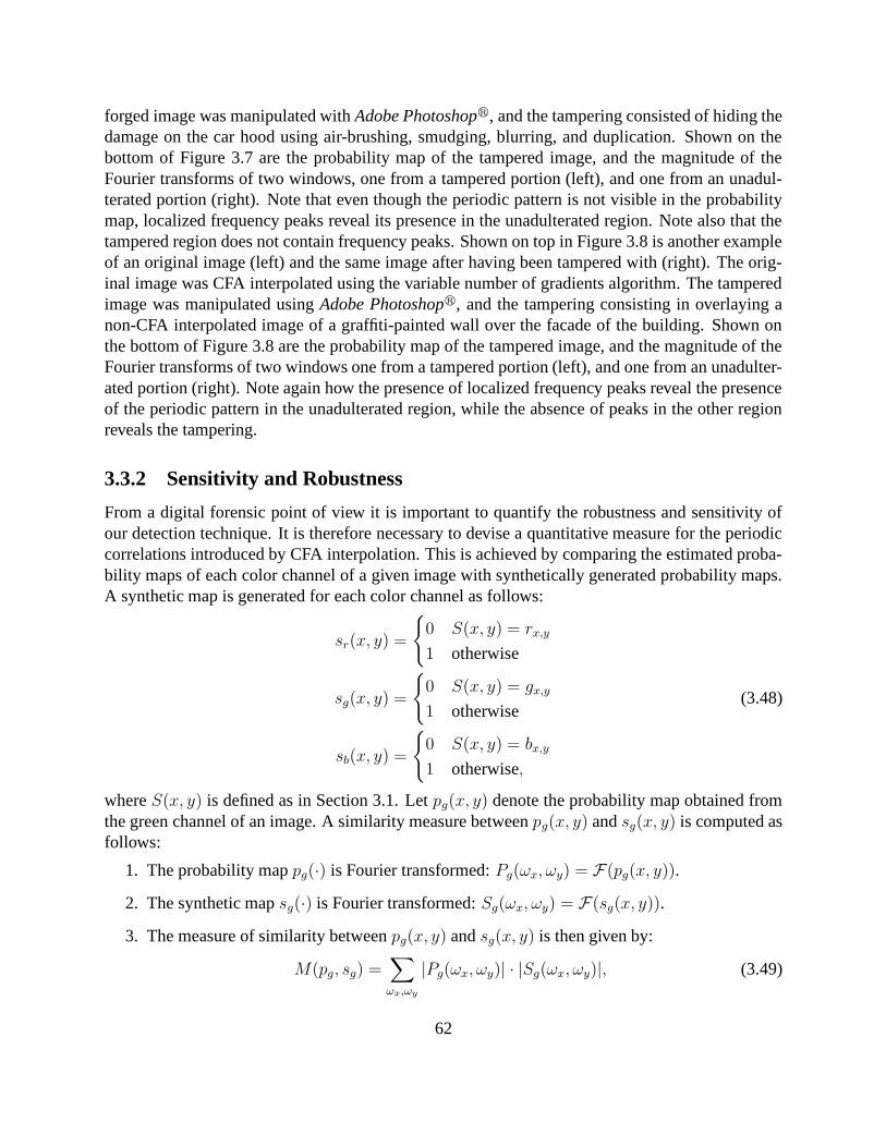
forged image was manipulated with Adobe Photoshopr, and the tampering consisted of hiding thedamage on the car hood using air-brushing, smudging, blurring, and duplication. Shown on thebottom of Figure 3.7 are the probability map of the tampered image, and the magnitude of theFourier transforms of two windows, one from a tampered portion (left), and one from an unadul-terated portion (right). Note that even though the periodic pattern is not visible in the probabilitymap, localized frequency peaks reveal its presence in the unadulterated region. Note also that thetampered region does not contain frequency peaks. Shown on top in Figure 3.8 is another exampleof an original image (left) and the same image after having been tampered with (right). The orig-inal image was CFA interpolated using the variable number of gradients algorithm. The tamperedimage was manipulated using Adobe Photoshopr, and the tampering consisting in overlaying anon-CFA interpolated image of a graffiti-painted wall over the facade of the building. Shown onthe bottom of Figure 3.8 are the probability map of the tampered image, and the magnitude of theFourier transforms of two windows one from a tampered portion (left), and one from an unadulter-ated portion (right). Note again how the presence of localized frequency peaks reveal the presenceof the periodic pattern in the unadulterated region, while the absence of peaks in the other regionreveals the tampering.


From a digital forensic point of view it is important to quantify the robustness and sensitivity ofour detection technique. It is therefore necessary to devise a quantitative measure for the periodiccorrelations introduced by CFA interpolation. This is achieved by comparing the estimated proba-bility maps of each color channel of a given image with synthetically generated probability maps.A synthetic map is generated for each color channel as follows:

sr(x, y) =

{

0 S(x, y) = rx,y

1 otherwise

sg(x, y) =

{

0 S(x, y) = gx,y

1 otherwise

sb(x, y) =

{

0 S(x, y) = bx,y

1 otherwise,

(3.48)

where S(x, y) is defined as in Section 3.1. Let pg(x, y) denote the probability map obtained fromthe green channel of an image. A similarity measure between pg(x, y) and sg(x, y) is computed asfollows:

1. The probability map pg(·) is Fourier transformed: Pg(ωx, ωy) = F(pg(x, y)).

2. The synthetic map sg(·) is Fourier transformed: Sg(ωx, ωy) = F(sg(x, y)).

3. The measure of similarity between pg(x, y) and sg(x, y) is then given by:

M(pg, sg) =∑

ωx,ωy

|Pg(ωx, ωy)| · |Sg(ωx, ωy)|, (3.49)

62

original tampered


Figure 3.7: Shown on top are an original (left) and a tampered image (right). Shown on the bottomare the probability map of the tampered image’s green channel, and the magnitude of the Fouriertransform of two windows from the probability map corresponding to a tampered (left) and unadul-terated (right) portion of the image. Note the lack of peaks in the tampered region signifying theabsence of CFA interpolation.

63

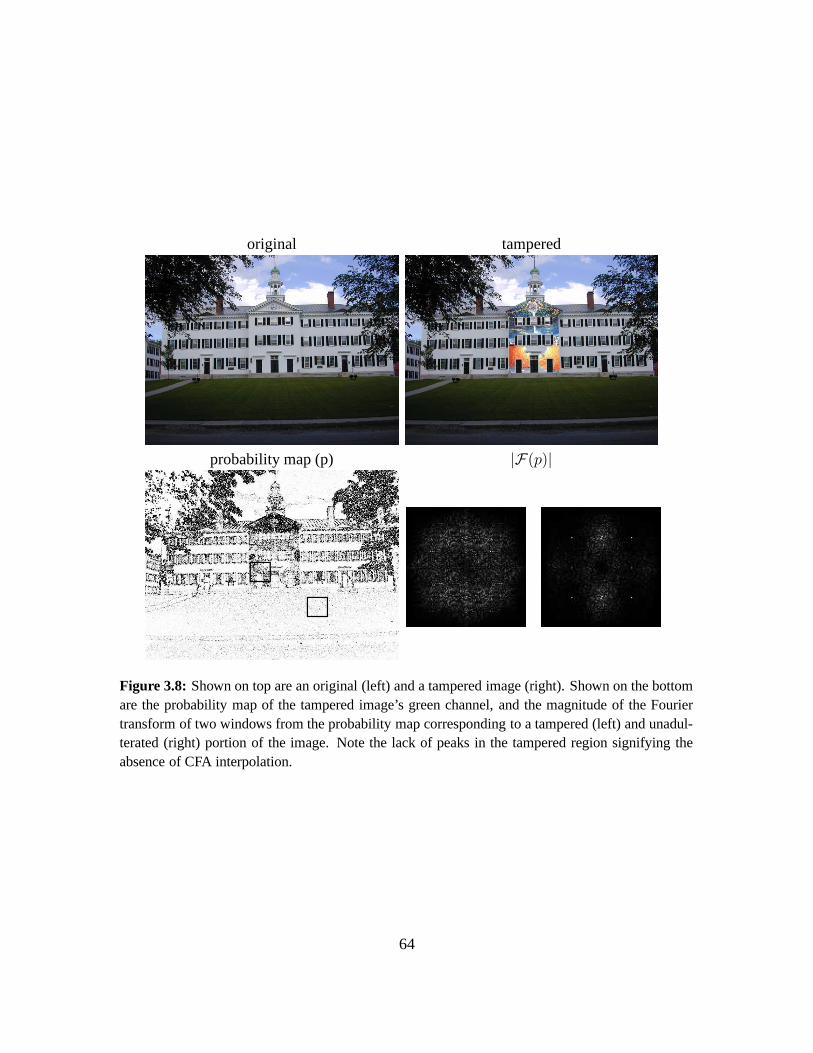
original tampered


Figure 3.8: Shown on top are an original (left) and a tampered image (right). Shown on the bottomare the probability map of the tampered image’s green channel, and the magnitude of the Fouriertransform of two windows from the probability map corresponding to a tampered (left) and unadul-terated (right) portion of the image. Note the lack of peaks in the tampered region signifying theabsence of CFA interpolation.

64

where | · | denotes absolute value (note that this similarity measure is phase insensitive).

The similarity measures between the probability and synthetic maps of the red and blue channels,M(pr, sr) and M(pb, sb), are computed in a similar way. If the similarity measure, M(pg, sg),between pg(x, y) and sg(x, y) is above a specified threshold, then a periodic pattern is assumed tobe present in the probability map, and the channel is labeled as CFA interpolated. Thresholds areempirically determined for each channel to yield a 0% false positive rate, i.e., no color channelfrom non-CFA interpolated images is classified as CFA interpolated.

To simulate tampering, each image in our database is blurred and down-sampled in order todestroy the original CFA interpolation correlations. These images are then re-sampled onto a BayerCFA and interpolated with each of the algorithms described in Section 3.1. Given a three-channelcolor image, we first compute the similarity measures between the probability maps of each colorchannel and the synthetic maps. The image is labeled as CFA interpolated if at least one of thethree similarities is greater than the specified thresholds, or as tampered if all three similaritiesare less than the thresholds. Using this approach, we have obtained, with a 0% false positive rate(i.e., a non-CFA interpolated image is never misclassified), the following classification accuraciesaveraged over 100 images:

bilinear bi-cubic smooth huemedian(3 × 3)

median(5 × 5)

gradient-based

adaptivecolorplane

variablenumber ofgradients

100% 100% 100% 99% 97% 100% 97% 100%

Counter Measures

To be useful in a forensic setting it is important for our detection method to be robust to counter-measures. We have tested the sensitivity of our method to simple counter attacks that may concealtraces of tampering: (1) lossy compression schemes (e.g., JPEG, GIF, and JPEG2000), (2) additivewhite Gaussian noise, and (3) non-linear point-wise gamma correction. Fifty images taken with theNikon Coolpix 950 camera, were processed as described in the previous section in order to obtainCFA and non-CFA interpolated images. Shown in Figure 3.9 are the detection accuracies (with 0%false positives) for different CFA interpolation algorithms as a function of the JPEG compressionquality. Note that these detection accuracies are close to 100% for quality factors greater than96 (out of 100), and that they decrease gracefully when the quality factors are decreasing. Thisdecrease in accuracy is expected, since the lossy JPEG compression introduces noise that interfereswith the correlations introduced by CFA interpolation. The decrease in accuracy depends on theCFA interpolation algorithm, e.g., at quality 70, the accuracy for smooth hue CFA interpolation is56%, while the accuracy for adaptive color plane CFA interpolation drops to 6%. We have alsotested our detection method on images that have been 8-bit color indexed (GIF). The detectionaccuracies (with 0% false positives) were perfect (i.e., 100%) for all CFA interpolation algorithms,except for the adaptive color plane interpolation, where the accuracy was 96%. Tests with imagescompressed with the JPEG2000 scheme revealed a weakness in our approach. The quantizationof wavelet coefficients employed by the JPEG2000 scheme, introduces periodic artifacts that are

65

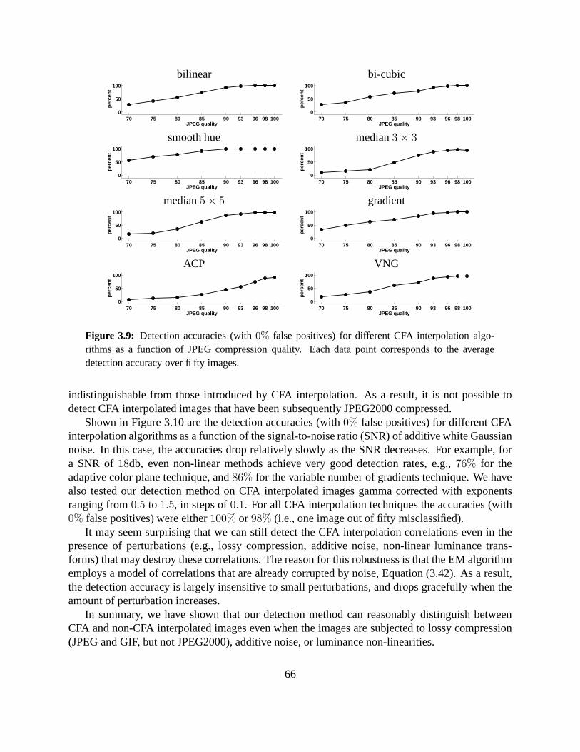
bilinear bi-cubic

70 75 80 85 90 93 96 98 1000

50

100

JPEG quality

per

cen

t

70 75 80 85 90 93 96 98 1000

50

100

JPEG quality

per

cen

t

smooth hue median 3 × 3

70 75 80 85 90 93 96 98 1000

50

100

JPEG quality

per

cen

t

70 75 80 85 90 93 96 98 1000

50

100

JPEG quality

per

cen

t

median 5 × 5 gradient

70 75 80 85 90 93 96 98 1000

50

100

JPEG quality

per

cen

t

70 75 80 85 90 93 96 98 1000

50

100

JPEG quality

per

cen

t

ACP VNG

70 75 80 85 90 93 96 98 1000

50

100

JPEG quality

per

cen

t

70 75 80 85 90 93 96 98 1000

50

100

JPEG quality

per

cen

t

Figure 3.9: Detection accuracies (with 0% false positives) for different CFA interpolation algo-rithms as a function of JPEG compression quality. Each data point corresponds to the averagedetection accuracy over fifty images.

indistinguishable from those introduced by CFA interpolation. As a result, it is not possible todetect CFA interpolated images that have been subsequently JPEG2000 compressed.

Shown in Figure 3.10 are the detection accuracies (with 0% false positives) for different CFAinterpolation algorithms as a function of the signal-to-noise ratio (SNR) of additive white Gaussiannoise. In this case, the accuracies drop relatively slowly as the SNR decreases. For example, fora SNR of 18db, even non-linear methods achieve very good detection rates, e.g., 76% for theadaptive color plane technique, and 86% for the variable number of gradients technique. We havealso tested our detection method on CFA interpolated images gamma corrected with exponentsranging from 0.5 to 1.5, in steps of 0.1. For all CFA interpolation techniques the accuracies (with0% false positives) were either 100% or 98% (i.e., one image out of fifty misclassified).

It may seem surprising that we can still detect the CFA interpolation correlations even in thepresence of perturbations (e.g., lossy compression, additive noise, non-linear luminance trans-forms) that may destroy these correlations. The reason for this robustness is that the EM algorithmemploys a model of correlations that are already corrupted by noise, Equation (3.42). As a result,the detection accuracy is largely insensitive to small perturbations, and drops gracefully when theamount of perturbation increases.

In summary, we have shown that our detection method can reasonably distinguish betweenCFA and non-CFA interpolated images even when the images are subjected to lossy compression(JPEG and GIF, but not JPEG2000), additive noise, or luminance non-linearities.

66

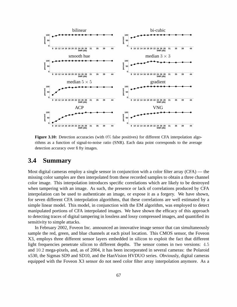
bilinear bi-cubic

8 10 12 14 16 18 20 22 24 26 28 31 35 39 440

50

100

SNR (db)

per

cen

t

8 10 12 14 16 18 20 22 24 26 28 31 35 39 440

50

100

SNR (db)

per

cen

t

smooth hue median 3 × 3

8 10 12 14 16 18 20 22 24 26 28 31 35 39 440

50

100

SNR (db)

per

cen

t

8 10 12 14 16 18 20 22 24 26 28 31 35 39 440

50

100

SNR (db)

per

cen

t

median 5 × 5 gradient

8 10 12 14 16 18 20 22 24 26 28 31 35 39 440

50

100

SNR (db)

per

cen

t

8 10 12 14 16 18 20 22 24 26 28 31 35 39 440

50

100

SNR (db)

per

cen

t

ACP VNG

8 10 12 14 16 18 20 22 24 26 28 31 35 39 440

50

100

SNR (db)

per

cen

t

8 10 12 14 16 18 20 22 24 26 28 31 35 39 440

50

100

SNR (db)

per

cen

t

Figure 3.10: Detection accuracies (with 0% false positives) for different CFA interpolation algo-rithms as a function of signal-to-noise ratio (SNR). Each data point corresponds to the averagedetection accuracy over fifty images.

3.4 Summary

Most digital cameras employ a single sensor in conjunction with a color filter array (CFA) — themissing color samples are then interpolated from these recorded samples to obtain a three channelcolor image. This interpolation introduces specific correlations which are likely to be destroyedwhen tampering with an image. As such, the presence or lack of correlations produced by CFAinterpolation can be used to authenticate an image, or expose it as a forgery. We have shown,for seven different CFA interpolation algorithms, that these correlations are well estimated by asimple linear model. This model, in conjunction with the EM algorithm, was employed to detectmanipulated portions of CFA interpolated images. We have shown the efficacy of this approachto detecting traces of digital tampering in lossless and lossy compressed images, and quantified itssensitivity to simple attacks.

In February 2002, Foveon Inc. announced an innovative image sensor that can simultaneouslysample the red, green, and blue channels at each pixel location. This CMOS sensor, the FoveonX3, employs three different sensor layers embedded in silicon to exploit the fact that differentlight frequencies penetrate silicon to different depths. The sensor comes in two versions: 4.5and 10.2 mega-pixels, and, as of 2004, it has been incorporated in several cameras: the Polaroidx530, the Sigmas SD9 and SD10, and the HanVision HVDUO series. Obviously, digital camerasequipped with the Foveon X3 sensor do not need color filter array interpolation anymore. As a

67

result, color images from these cameras will no longer exhibit the periodic correlations specific tocolor filter array interpolated images, and our detection method will not be applicable. We expect,however, that our technique would still prove worthwhile in the future given that single sensorcameras constitute the vast majority of the market today, and are likely to remain cheaper, andmore available to average users.

As with any authentication scheme, our approach is vulnerable to counter-attack. A tamperedimage could, for example, be re-sampled onto a CFA, and then re-interpolated. This attack, how-ever, requires knowledge of the camera’s CFA pattern and interpolation algorithm, and is likely tobe beyond the reaches of a novice forger.

68

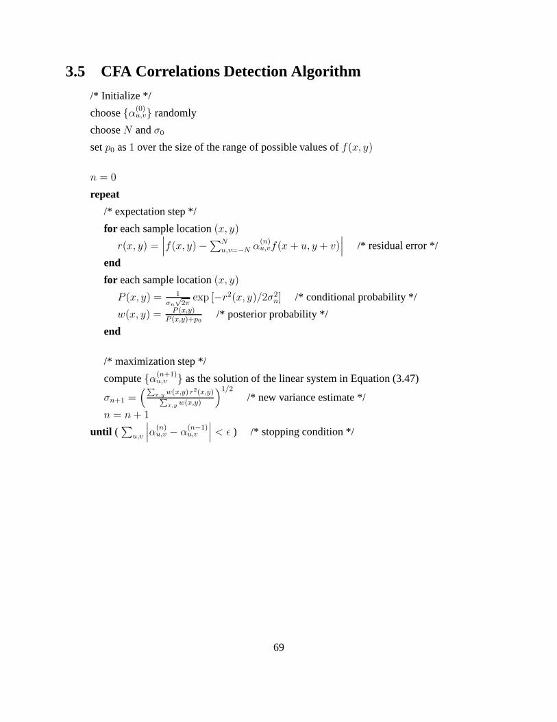
3.5 CFA Correlations Detection Algorithm

/* Initialize */

choose {α(0)u,v} randomly

choose N and σ0

set p0 as 1 over the size of the range of possible values of f(x, y)

n = 0

repeat

/* expectation step */

for each sample location (x, y)

r(x, y) =∣

∣

∣f(x, y) −∑N

u,v=−N α(n)u,vf(x + u, y + v)

∣

∣

∣/* residual error */

end

for each sample location (x, y)

P (x, y) = 1σn

√2π

exp [−r2(x, y)/2σ2n] /* conditional probability */

w(x, y) = P (x,y)P (x,y)+p0

/* posterior probability */

end

/* maximization step */

compute {α(n+1)u,v } as the solution of the linear system in Equation (3.47)

σn+1 =(P

x,y w(x,y) r2(x,y)P

x,y w(x,y)

)1/2

/* new variance estimate */

n = n + 1

until (∑

u,v

∣

∣

∣α

(n)u,v − α

(n−1)u,v

∣

∣

∣< ε ) /* stopping condition */

69

Chapter 4

Double JPEG Compression

Tampering with a digital image generally requires the use of a photo-editing software package,such as Adobe Photoshopr. When creating digital forgeries, an image is loaded into the photo-editing software, some manipulations are performed, and the image is re-saved. If JPEG format isused to store the images (a majority of digital cameras have as default setting the option to storeimages directly in JPEG format) the tampered image has been double JPEG compressed. Doublecompressed images contain specific artifacts1 that can be employed to distinguish them from singlecompressed images. Note, however, that detecting double JPEG compression does not necessarilyprove malicious tampering: it is possible, for example, that a user may re-save high quality JPEGimages with lower quality to save storage space. The authenticity of a double JPEG compressedimage, however, is at least questionable and further analysis would be required.

We start by giving a brief description of the JPEG compression algorithm. Next, we describethe specific artifacts introduced by double JPEG compression and illustrate them on several ex-amples of natural images. Finally, we propose a method for detecting and quantifying doublecompressed images and analyze its sensitivity on a database of 100 natural images.

4.1 JPEG Compression

JPEG is a standardized image compression procedure proposed by a committee with the samename JPEG (Joint Photographic Experts Committee). To be generally applicable, the JPEG stan-dard [1] specified two compression schemes: a lossless predictive scheme and a lossy schemebased on the discrete cosine transform (DCT). The most popular lossy compression technique isknown as the baseline method and encompasses a subset of the DCT-based modes of operation. Inthis section, a summary of the baseline method will be presented.

The encoding procedure consists of three sequential steps [59], and yields a compressed streamof data:

1. Discrete Cosine Transform (DCT): image samples are grouped into 8 × 8 blocks in raster

1The fact that specific artifacts are present in double JPEG compressed images was also independently noticedin [39].

70

scan order (left to right, top to bottom) and shifted from unsigned to signed integers (i.e.,from range [0, 255] to [−128, 127]), then the DCT of the blocks is computed. Let f(x, y)denote an 8 × 8 image block, then its DCT takes the form:

F (ωx, ωy) =1

4c(ωx)c(ωy)

7∑

x=0

7∑

y=0

f(x, y) cos(2x + 1)ωxπ

16cos

(2y + 1)ωyπ

16,

ωx, ωy = 0, . . . , 7, (4.1)

where c(ω) = 1/√

2, for ω = 0, and c(ω) = 1 otherwise.

2. Quantization: The DCT coefficients obtained in the previous step are uniformly quantized.The reason for quantization is to represent the DCT coefficients with no greater precisionthan necessary for a desired visual quality. Quantization is a point-wise operation defined asdivision by a quantization step followed by rounding to the nearest integer:

Fq(ωx, ωy) =

⌊

F (ωx, ωy)

s(ωx, ωy)+

1

2

⌋

, ωx, ωy = 0, . . . , 7, (4.2)

where s(ωx, ωy) is a frequency dependent quantization step. The relationship between theJPEG quality, Q, and the quantization steps s(ωx, ωy) takes the form:

s(ωx, ωy) =

max(⌊

200−2Q100

C(ωx, ωy) + 12

⌋

, 1)

, 50 ≤ Q ≤ 100

⌊

50Q

C(ωx, ωy) + 12

⌋

, 0 < Q < 50,

(4.3)

where C(ωx, ωy) are experimentally determined to be:

C(ωx, ωy) =

16 11 10 16 24 40 51 6112 12 14 19 26 58 60 5514 13 16 24 40 57 69 5614 17 22 29 51 87 80 6218 22 37 56 68 109 103 7724 35 55 64 81 104 113 9249 64 78 87 103 121 120 10172 92 95 98 112 100 103 99

. (4.4)

In Equation (4.4), the upper left value (16) corresponds to the DC term, and the bottom rightvalue (99) corresponds to the highest horizontal and vertical frequencies. The upper rightvalue (61) corresponds to the highest vertical frequency, and lowest horizontal frequency,while the bottom left value (72) corresponds to the highest horizontal frequency, and lowest

71

vertical frequency. These values were determined experimentally to yield a good trade-off between compression and perceptual quality. Note that quantization is a non-invertibleoperation, therefore causing loss of information. This step represents the main source ofinformation loss in the DCT-based JPEG compression scheme.

3. Entropy Encoding: This step involves lossless entropy compression that transforms thequantized DCT coefficients into a stream of compressed data. The most frequently usedprocedure is Huffman coding, although arithmetic coding is also supported.

The decoding of a compressed data stream involves the inverse of the previous three steps, takenin reverse order:

1. Entropy Decoding: The compressed data stream is decoded to recover the quantized DCTcoefficients.

2. De-quantization: For each 8 × 8 block, the quantized DCT coefficients are multiplied bytheir corresponding quantization steps:

F (ωx, ωy) = Fq(ωx, ωy)s(ωx, ωy), ωx, ωy = 0, . . . , 7, (4.5)

where s(ωx, ωy) is defined in Equation (4.3).

3. Inverse Discrete Cosine Transform (IDCT): The IDCT of the de-quantized DCT coeffi-cients, F (ωx, ωy), is first computed, then the result is shifted back to the range [0, 255] toobtain reconstructed 8 × 8 image blocks. Let f(x, y) denote a reconstructed image blockobtained from IDCT:

f(x, y) =1

4

7∑

ωx=0

7∑

ωy=0

c(ωx)c(ωy)F (ωx, ωy) cos(2x + 1)ωxπ

16cos

(2y + 1)ωyπ

16,

x, y = 0, . . . , 7, (4.6)

where c(ω) = 1/√

2, for ω = 0, and c(ω) = 1 otherwise.

For simplicity, only the case of sequential compression of single channel images (gray-scale)has been presented. Three-channel (color) images are first converted to a luminance-chrominancecolor space [2], the chrominance channels are down-sampled by a factor of two, then the gray-scalecompression method is independently applied to the luminance and chrominance channels2.

Note that double JPEG compression amounts to double quantization of block DCT coefficients.We will show next that the double quantization of a signal of any type (e.g., a sequence of DCTcoefficients) introduces specific artifacts that can be quantified and detected.

2For the luminance channel the quantization table for gray-scale images, Equation (4.4), is employed. A differentquantization table is employed for the chrominance channels.

72

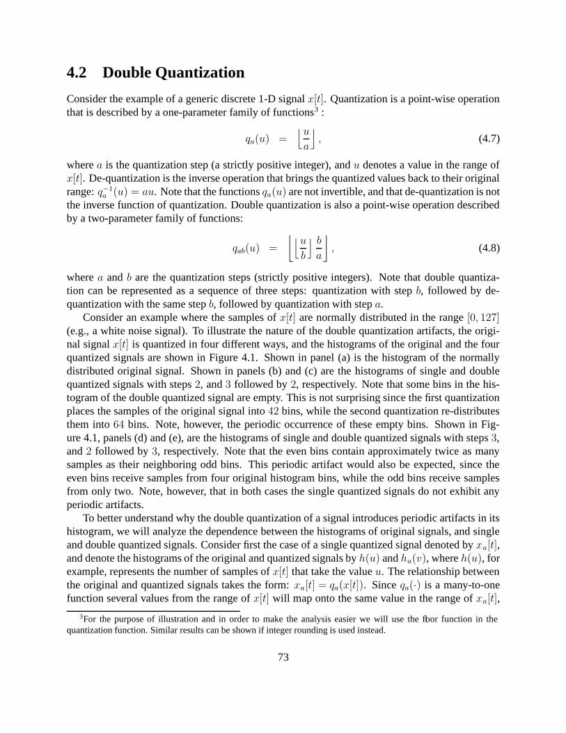
4.2 Double Quantization

Consider the example of a generic discrete 1-D signal x[t]. Quantization is a point-wise operationthat is described by a one-parameter family of functions3 :

qa(u) =⌊u

a

⌋

, (4.7)

where a is the quantization step (a strictly positive integer), and u denotes a value in the range ofx[t]. De-quantization is the inverse operation that brings the quantized values back to their originalrange: q−1

a (u) = au. Note that the functions qa(u) are not invertible, and that de-quantization is notthe inverse function of quantization. Double quantization is also a point-wise operation describedby a two-parameter family of functions:

qab(u) =

⌊

⌊u

b

⌋ b

a

⌋

, (4.8)

where a and b are the quantization steps (strictly positive integers). Note that double quantiza-tion can be represented as a sequence of three steps: quantization with step b, followed by de-quantization with the same step b, followed by quantization with step a.

Consider an example where the samples of x[t] are normally distributed in the range [0, 127](e.g., a white noise signal). To illustrate the nature of the double quantization artifacts, the origi-nal signal x[t] is quantized in four different ways, and the histograms of the original and the fourquantized signals are shown in Figure 4.1. Shown in panel (a) is the histogram of the normallydistributed original signal. Shown in panels (b) and (c) are the histograms of single and doublequantized signals with steps 2, and 3 followed by 2, respectively. Note that some bins in the his-togram of the double quantized signal are empty. This is not surprising since the first quantizationplaces the samples of the original signal into 42 bins, while the second quantization re-distributesthem into 64 bins. Note, however, the periodic occurrence of these empty bins. Shown in Fig-ure 4.1, panels (d) and (e), are the histograms of single and double quantized signals with steps 3,and 2 followed by 3, respectively. Note that the even bins contain approximately twice as manysamples as their neighboring odd bins. This periodic artifact would also be expected, since theeven bins receive samples from four original histogram bins, while the odd bins receive samplesfrom only two. Note, however, that in both cases the single quantized signals do not exhibit anyperiodic artifacts.

To better understand why the double quantization of a signal introduces periodic artifacts in itshistogram, we will analyze the dependence between the histograms of original signals, and singleand double quantized signals. Consider first the case of a single quantized signal denoted by xa[t],and denote the histograms of the original and quantized signals by h(u) and ha(v), where h(u), forexample, represents the number of samples of x[t] that take the value u. The relationship betweenthe original and quantized signals takes the form: xa[t] = qa(x[t]). Since qa(·) is a many-to-onefunction several values from the range of x[t] will map onto the same value in the range of xa[t],

3For the purpose of illustration and in order to make the analysis easier we will use the floor function in thequantization function. Similar results can be shown if integer rounding is used instead.

73

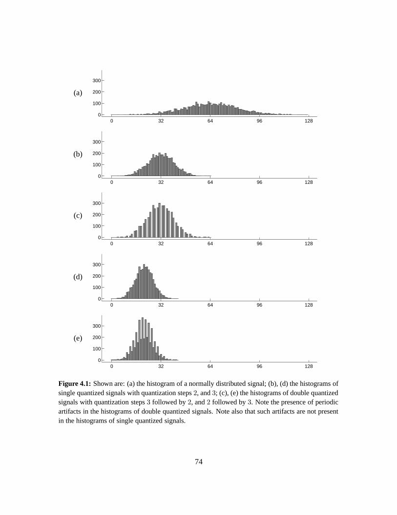
(a)

0 32 64 96 1280

100

200

300

(b)

0 32 64 96 1280

100

200

300

(c)

0 32 64 96 1280

100

200

300

(d)

0 32 64 96 1280

100

200

300

(e)

0 32 64 96 1280

100

200

300

Figure 4.1: Shown are: (a) the histogram of a normally distributed signal; (b), (d) the histograms ofsingle quantized signals with quantization steps 2, and 3; (c), (e) the histograms of double quantizedsignals with quantization steps 3 followed by 2, and 2 followed by 3. Note the presence of periodicartifacts in the histograms of double quantized signals. Note also that such artifacts are not presentin the histograms of single quantized signals.

74

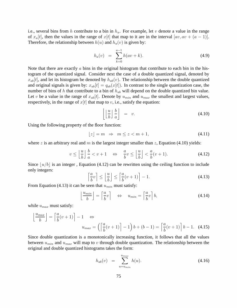
i.e., several bins from h contribute to a bin in ha. For example, let v denote a value in the rangeof xa[t], then the values in the range of x[t] that map to it are in the interval [av, av + (a − 1)].Therefore, the relationship between h(u) and ha(v) is given by:

ha(v) =a−1∑

k=0

h(av + k). (4.9)

Note that there are exactly a bins in the original histogram that contribute to each bin in the his-togram of the quantized signal. Consider next the case of a double quantized signal, denoted byxab[t], and let its histogram be denoted by hab(v). The relationship between the double quantizedand original signals is given by: xab[t] = qab(x[t]). In contrast to the single quantization case, thenumber of bins of h that contribute to a bin of hab will depend on the double quantized bin value.Let v be a value in the range of xab[t]. Denote by umin and umax the smallest and largest values,respectively, in the range of x[t] that map to v, i.e., satisfy the equation:

⌊

⌊u

b

⌋ b

a

⌋

= v. (4.10)

Using the following property of the floor function:

bzc = m ⇒ m ≤ z < m + 1, (4.11)

where z is an arbitrary real and m is the largest integer smaller than z, Equation (4.10) yields:

v ≤⌊u

b

⌋ b

a< v + 1 ⇔ a

bv ≤

⌊u

b

⌋

<a

b(v + 1). (4.12)

Since bu/bc is an integer , Equation (4.12) can be rewritten using the ceiling function to includeonly integers:

⌈a

bv⌉

≤⌊u

b

⌋

≤⌈a

b(v + 1)

⌉

− 1. (4.13)

From Equation (4.13) it can be seen that umin must satisfy:⌊umin

b

⌋

=⌈a

bv⌉

⇔ umin =⌈a

bv⌉

b, (4.14)

while umax must satisfy:⌊umax

b

⌋

=⌈a

b(v + 1)

⌉

− 1 ⇔

umax =(⌈a

b(v + 1)

⌉

− 1)

b + (b − 1) =⌈a

b(v + 1)

⌉

b − 1. (4.15)

Since double quantization is a monotonically increasing function, it follows that all the valuesbetween umin and umax will map to v through double quantization. The relationship between theoriginal and double quantized histograms takes the form:

hab(v) =umax∑

u=umin

h(u). (4.16)

75

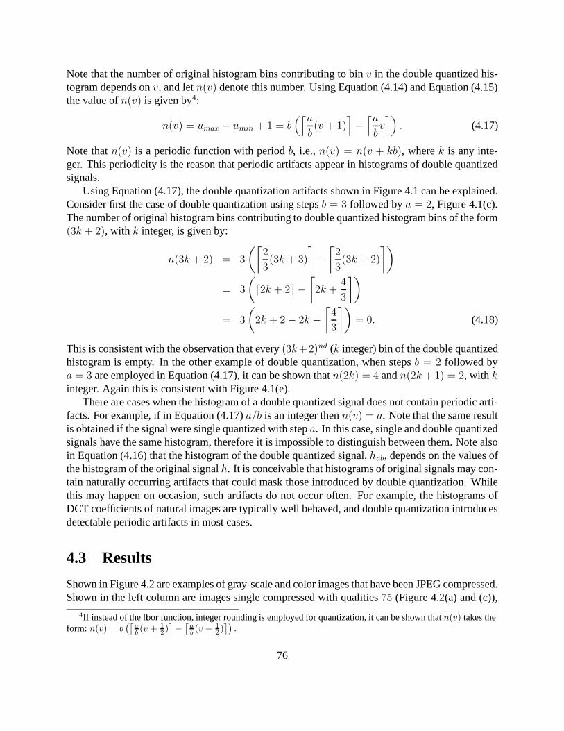
Note that the number of original histogram bins contributing to bin v in the double quantized his-togram depends on v, and let n(v) denote this number. Using Equation (4.14) and Equation (4.15)the value of n(v) is given by4:

n(v) = umax − umin + 1 = b(⌈a

b(v + 1)

⌉

−⌈a

bv⌉)

. (4.17)

Note that n(v) is a periodic function with period b, i.e., n(v) = n(v + kb), where k is any inte-ger. This periodicity is the reason that periodic artifacts appear in histograms of double quantizedsignals.

Using Equation (4.17), the double quantization artifacts shown in Figure 4.1 can be explained.Consider first the case of double quantization using steps b = 3 followed by a = 2, Figure 4.1(c).The number of original histogram bins contributing to double quantized histogram bins of the form(3k + 2), with k integer, is given by:

n(3k + 2) = 3

(⌈

2

3(3k + 3)

⌉

−⌈

2

3(3k + 2)

⌉)

= 3

(

d2k + 2e −⌈

2k +4

3

⌉)

= 3

(

2k + 2 − 2k −⌈

4

3

⌉)

= 0. (4.18)

This is consistent with the observation that every (3k+2)nd (k integer) bin of the double quantizedhistogram is empty. In the other example of double quantization, when steps b = 2 followed bya = 3 are employed in Equation (4.17), it can be shown that n(2k) = 4 and n(2k + 1) = 2, with kinteger. Again this is consistent with Figure 4.1(e).

There are cases when the histogram of a double quantized signal does not contain periodic arti-facts. For example, if in Equation (4.17) a/b is an integer then n(v) = a. Note that the same resultis obtained if the signal were single quantized with step a. In this case, single and double quantizedsignals have the same histogram, therefore it is impossible to distinguish between them. Note alsoin Equation (4.16) that the histogram of the double quantized signal, hab, depends on the values ofthe histogram of the original signal h. It is conceivable that histograms of original signals may con-tain naturally occurring artifacts that could mask those introduced by double quantization. Whilethis may happen on occasion, such artifacts do not occur often. For example, the histograms ofDCT coefficients of natural images are typically well behaved, and double quantization introducesdetectable periodic artifacts in most cases.

4.3 Results

Shown in Figure 4.2 are examples of gray-scale and color images that have been JPEG compressed.Shown in the left column are images single compressed with qualities 75 (Figure 4.2(a) and (c)),

4If instead of the floor function, integer rounding is employed for quantization, it can be shown that n(v) takes theform: n(v) = b

(⌈

ab(v + 1

2 )⌉

−⌈

ab(v − 1

2 )⌉)

.

76

and 85 (Figure 4.2(b) and (d)), and in the middle column are the same images images doublecompressed with qualities 85 followed by 75 (Figure 4.2(a) and (c)), and 75 followed by 85 (Fig-ure 4.2(b) and (d)). Also shown in the right column are the absolute differences between the singleand double compressed images5. Note that although there is little perceptual difference betweenthe single and double compressed images, double compression introduces band-pass noise with asignal-to-noise ratio ranging between 20db and 24dB. Since double JPEG compression amountsto double quantization of DCT coefficients of image blocks, the histograms of these coefficientswill contain periodic artifacts, as explained in Section 4.2. For example, shown in Figure 4.3 arethe DCT coefficients, their histograms and the Fourier transforms of the zero-mean histograms ofthe gray-scale images in Figure 4.2(a). Shown in Figure 4.3(a)-(b) are the DCT coefficients of thesingle JPEG compressed image with quality 75, while in Figure 4.3(c)-(d) are the DCT coefficientsof the double JPEG compressed image with qualities 85 followed by 75. The DCT coefficients areshown as images (auto-scaled to fill the full intensity range), where each pixel corresponds to a8 × 8 block in the JPEG compressed images, and the intensities represent the coefficient values.The coefficients in Figure 4.3(a) and (c) correspond to DCT frequency (1, 1), the DC component,and the coefficients in Figure 4.3(b) and (d) correspond to DCT frequency (2, 2). In a way simi-lar to Figure 4.3, Figures 4.4-4.6 contain the DCT coefficients6, their histograms and the Fouriertransforms of the zero-mean histograms of the images in Figure 4.2(b)-(d). Note that periodicartifacts are present in the histograms of the DCT coefficients of the double compressed images.These artifacts are particularly visible in the Fourier transforms of the histograms in the form ofstrong peaks in the mid and high frequencies. Note that for single compressed images no periodicartifacts or high-frequency peaks are present.

The periodic patterns introduced by double JPEG compression depend on the quality parame-ters. As a result, it is possible to detect not only if an image has been double compressed, but alsothe compression qualities that have been used. The second parameter can be found from the quan-tization table stored in the JPEG file, while the first parameter can be inferred from the location ofthe frequency peaks in the Fourier transform of the DCT coefficient histograms.

4.3.1 Quantifying Double JPEG Compression Artifacts

For forensics applications, it is important to quantify the sensitivity and robustness of our approachfor detecting double JPEG compression. To this end it is first necessary to devise a quantitativemeasure for the periodic artifacts introduced in the DCT coefficient histograms. The purposeof this measure is to discriminate between single and double quantized coefficients, e.g., highvalues would correspond to double quantization, while low values would correspond to singlequantization.

Consider a sequence of DCT coefficients known to have been double quantized with steps bfollowed by a. If a/b does not have an integer value, Section 4.2, double quantization introduces inthe DCT coefficient histogram periodic artifacts that have a specific peak pattern in the frequency

5For display purposes, these absolute differences have been auto-scaled to fill the full intensity range, and gammacorrected with γ = 0.75.

6For color images the DCT coefficients of the luminance channel are shown.

77

single compressed double compressed absolute difference

(a)

(b)

(c)

(d)

Figure 4.2: Shown on the left are four images single JPEG compressed with qualities 75, (a) and(c), and 85, (b) and (d). Shown in the middle are the same images double JPEG compressed withqualities 85 followed by 75, (a) and (c), and 75 followed by 85, (b) and (d). Shown on the right arethe absolute differences of the single and double JPEG compressed images (for display purposes,these differences were gamma corrected with γ = 0.75, and auto-scaled to fill the full intensityrange). See also Figures 4.3-4.6.

78

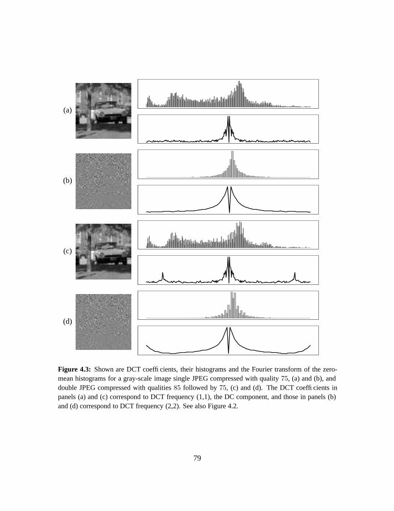
(a)

(b)

(c)

(d)

Figure 4.3: Shown are DCT coefficients, their histograms and the Fourier transform of the zero-mean histograms for a gray-scale image single JPEG compressed with quality 75, (a) and (b), anddouble JPEG compressed with qualities 85 followed by 75, (c) and (d). The DCT coefficients inpanels (a) and (c) correspond to DCT frequency (1,1), the DC component, and those in panels (b)and (d) correspond to DCT frequency (2,2). See also Figure 4.2.

79

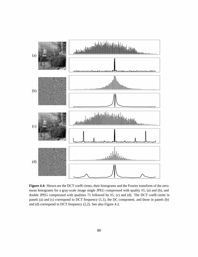
(a)

(b)

(c)

(d)

Figure 4.4: Shown are the DCT coefficients, their histograms and the Fourier transform of the zero-mean histograms for a gray-scale image single JPEG compressed with quality 85, (a) and (b), anddouble JPEG compressed with qualities 75 followed by 85, (c) and (d). The DCT coefficients inpanels (a) and (c) correspond to DCT frequency (1,1), the DC component, and those in panels (b)and (d) correspond to DCT frequency (2,2). See also Figure 4.2.

80

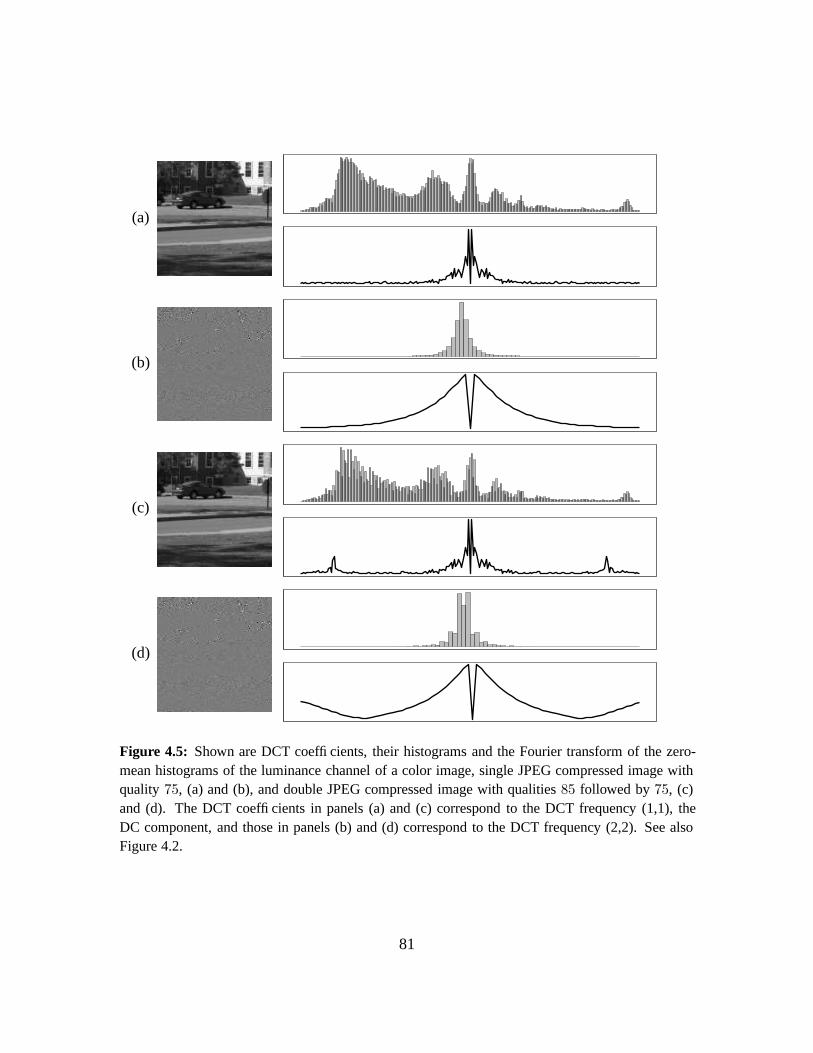
(a)

(b)

(c)

(d)

Figure 4.5: Shown are DCT coefficients, their histograms and the Fourier transform of the zero-mean histograms of the luminance channel of a color image, single JPEG compressed image withquality 75, (a) and (b), and double JPEG compressed image with qualities 85 followed by 75, (c)and (d). The DCT coefficients in panels (a) and (c) correspond to the DCT frequency (1,1), theDC component, and those in panels (b) and (d) correspond to the DCT frequency (2,2). See alsoFigure 4.2.

81

(a)

(b)

(c)

(d)

Figure 4.6: Shown are the DCT coefficients, their histograms and the Fourier transform of thezero-mean histograms of the luminance channel of a color image, single JPEG compressed imagewith quality 85, (a) and (b), and double JPEG compressed image with qualities 75 followed by 85,(c) and (d). The DCT coefficients in panels (a) and (c) correspond to the DCT frequency (1,1), theDC component, and those in panels (b) and (d) correspond to the DCT frequency (2,2). See alsoFigure 4.2.

82

domain. This pattern can be estimated by taking a signal drawn from a uniform distribution,double quantizing it with the same steps (b followed by a), computing the Fourier transform of thedouble quantized signal’s histogram, and finding the peak locations. A quantitative measure forthe periodicity of the DCT coefficients’ histogram is then obtained by averaging the energy valuesin the frequency domain at the peak locations. More specifically, denoting with hab(v) and uab(v)the histograms of the DCT coefficients and of the double quantized, uniformly distributed signal,respectively, the quantitative measure is computed as follows:

1. The histograms hab and uab are Fourier transformed:

Hab(ω) = hab(v) Uab(ω) = uab(v). (4.19)

2. The double quantization peaks are located in Uab(ω) by selecting the values above a thresh-old. Let P denote the set of peak locations in the frequency domain:

P = {ω | Uab(ω) ≥ Et}, (4.20)

where Et is an empirically chosen threshold7.

3. The Fourier transform of the DCT coefficient histogram typically contains a decaying trendthat interferes with the peaks introduced by double quantization. This trend needs to beremoved in order to obtain an accurate measurement of the peaks’ energy. We have empiri-cally found that a two-parameter generalized Laplace model approximates well, in general,the shape of this trend8:

L(ω; α, β) = e−|ω|α/β. (4.21)

The model parameters are estimated through non-linear minimization to be optimal in theleast squares sense: (α?, β?) = arg min(α,β) E(α, β), where the quadratic error functionE(α, β) takes the form:

E(α, β) =∑

ω 6∈P

(Hab(ω) − L(ω; α, β))2 . (4.22)

Note that, in order to avoid the interference of the double quantization peaks, only the valuesat non-peak locations, ω 6∈ P , are employed in the computation of the error function.

The decaying trend is removed by subtracting the generalized Laplace model, L(ω; α?, β?),from Hab(ω) and taking the square to avoid negative values:

Dab(ω) = (Hab(ω) − L(ω; α?, β?))2. (4.23)

7For our experiments we have chosen Et to be the 85th percentile of the values of Uab(ω).8The generalized Laplace model, also known as generalized Gaussian or stretched exponential, has been used in

the past to model the marginal densities of wavelet coefficients [42, 57, 45]. The exact form of the generalized Laplace

distribution is given by e−|x/s|p

Z(s,p) , where the normalizing factor is Z(s, p) = 2 spΓ(

1p

)

, with the generalized factorial

gamma function given by: Γ(z) =∫

∞

0tz−1e−tdt.

83

4. From Dab(ω) the periodicity measure is computed as a weighted average at the peak loca-tions in P :

M(hab; a, b) =

∑

ω W (ω)Dab(ω)∑

ω W (ω), (4.24)

where the weights W (ω) are given by:

W (ω) =

{

Uab(ω) ω ∈ P

0 ω 6∈ P.(4.25)

Note that the measure in Equation (4.24) depends on the histogram of the DCT coefficients,hab as well as on the quantization steps, a and b. Since in general the first quantization step, b, isunknown, a measure that is independent of b is obtained by taking the maximum over all detectablevalues of b:

M(hab; a) = maxb∈Ba

M(hab; a, b), (4.26)

where the set of all detectable first steps is given by: Ba = {b | a/b 6∈ N, b ≤ bmax}, where bmax isa positive integer.

Consider a sequence of DCT coefficients known to be quantized with step a and let h(v) denoteits histogram. If the value of the measure, M(h; a), is above a specified threshold, it is assumedthat double quantization periodic artifacts are present in the DCT coefficient histogram and theDCT coefficients are labeled as double quantized. The threshold is empirically determined fromsingle quantized DCT coefficients so that a desired false positive rate is obtained.

Shown in Figures 4.7-4.8, panels (a)-(d), are the histograms and their Fourier transforms fora sequence of DCT coefficients, and for a signal drawn from a uniform distribution that havebeen both double quantized with steps 3 followed by 7, and 4 followed by 7, respectively. TheDCT coefficients correspond to DCT frequencies (2, 1) and (1, 2), and have been taken from theluminance channel of images double JPEG compressed with qualities 85, followed by 70. Note thatthe high frequency peaks appear at the same locations in the Fourier transforms of both histograms.Note also that the spectrum of the double quantized uniform distribution histogram is flat exceptat the locations of the peaks, while the spectrum of the DCT coefficient histogram contains adecaying trend. Shown in Figures 4.7-4.8, panels (e)-(f), are the generalized Laplace models of theDCT coefficient spectra and the square differences between the spectra and the models. The valuesof the optimal (in the least squares sense) model parameters were: α = 0.94961, β = 6.3683 forFigure 4.7(e), and α = 1.2316, β = 5.3878 for Figure 4.8(e). Note the similarity between thespectra of the double quantized uniform distributions, on one hand, and the difference betweenthe DCT coefficient spectra and their models, on the other hand. The values used to compute theweighted average in Equation (4.24) are indicated by the bigger white dots in panels (d) and (f) ofFigures 4.7-4.8.


With the ability to quantitatively measure the double quantization periodic artifacts, we have de-vised a simple scheme to detect double JPEG compressed images. Given a JPEG compressed

84

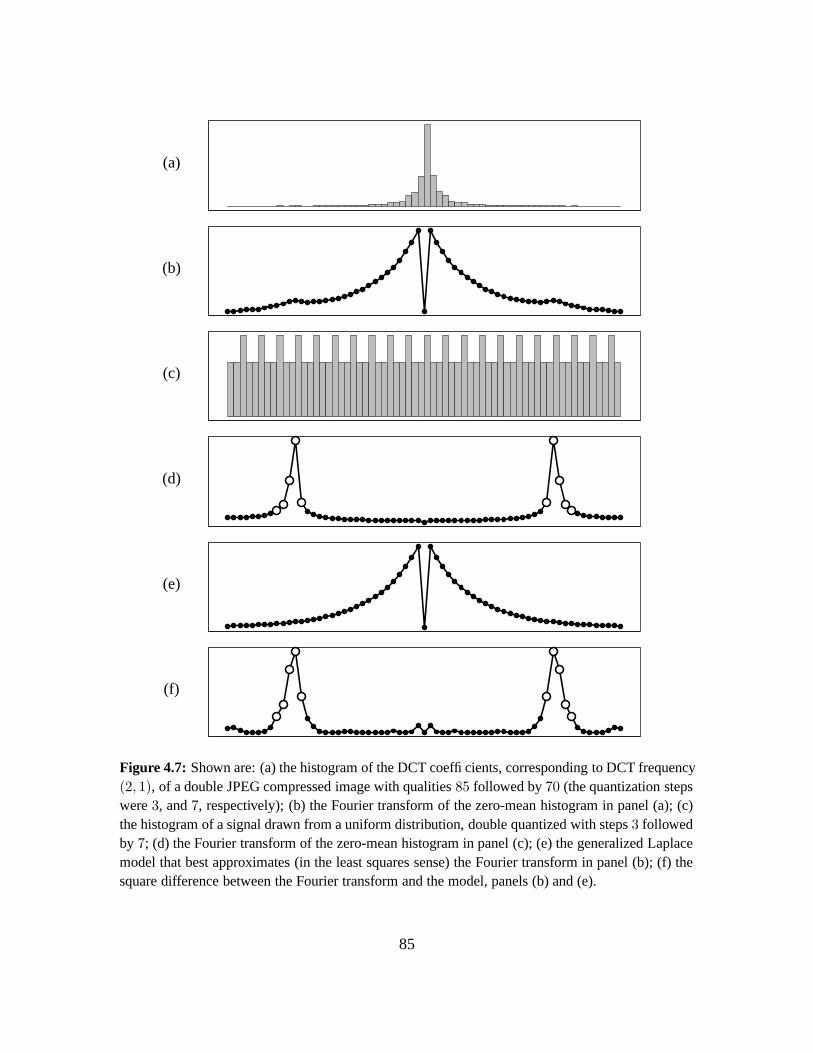
(a)

(b)

(c)

(d)

(e)

(f)

Figure 4.7: Shown are: (a) the histogram of the DCT coefficients, corresponding to DCT frequency(2, 1), of a double JPEG compressed image with qualities 85 followed by 70 (the quantization stepswere 3, and 7, respectively); (b) the Fourier transform of the zero-mean histogram in panel (a); (c)the histogram of a signal drawn from a uniform distribution, double quantized with steps 3 followedby 7; (d) the Fourier transform of the zero-mean histogram in panel (c); (e) the generalized Laplacemodel that best approximates (in the least squares sense) the Fourier transform in panel (b); (f) thesquare difference between the Fourier transform and the model, panels (b) and (e).

85

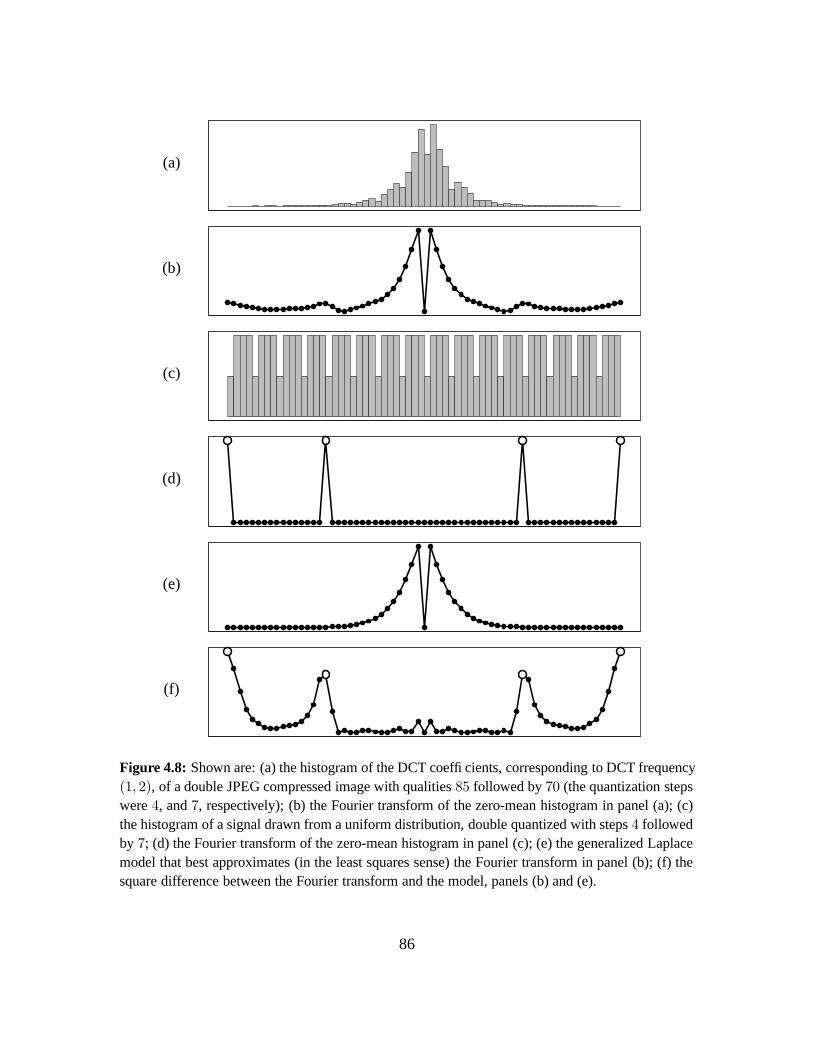
(a)

(b)

(c)

(d)

(e)

(f)

Figure 4.8: Shown are: (a) the histogram of the DCT coefficients, corresponding to DCT frequency(1, 2), of a double JPEG compressed image with qualities 85 followed by 70 (the quantization stepswere 4, and 7, respectively); (b) the Fourier transform of the zero-mean histogram in panel (a); (c)the histogram of a signal drawn from a uniform distribution, double quantized with steps 4 followedby 7; (d) the Fourier transform of the zero-mean histogram in panel (c); (e) the generalized Laplacemodel that best approximates (in the least squares sense) the Fourier transform in panel (b); (f) thesquare difference between the Fourier transform and the model, panels (b) and (e).

86

Q2 50 55 60 65 70 75 80 85 90 95

Q1

50 – 100% 100% 100% 100% 100% 100% 100% 100% 100%

55 70% – 99% 100% 100% 100% 100% 100% 100% 100%

60 98% 85% – 100% 100% 100% 100% 100% 100% 100%

65 100% 100% 100% – 100% 100% 100% 100% 100% 100%

70 100% 100% 100% 97% – 100% 100% 100% 100% 100%

75 93% 100% 100% 100% 100% – 100% 100% 100% 100%

80 96% 100% 98% 100% 100% 100% – 100% 100% 100%

85 74% 65% 100% 98% 100% 100% 100% – 100% 100%

90 48% 63% 78% 89% 99% 100% 100% 100% – 100%

95 N/D N/D 73% 98% N/D N/D N/D 100% 100% –

Table 4.1: Detection accuracy with 0% false positive rate for double JPEG compressed images. Thefirst quality is held constant on the rows, while the second quality is held constant on the columns.The N/D (not detectable) table entries correspond to pairs of qualities that yield double compressedimages indistinguishable from single compressed images. Each accuracy value corresponds to anaverage over 100 images. See also Figure 4.9.

image, we first extract the coefficients of a subset of DCT frequencies, and the quantization tablestored in the JPEG file. Next, we employ the periodicity measure defined in the previous section,Equation (4.26), to check if there are double quantized coefficients. If the coefficients of at leastone DCT frequency are double quantized, the image is labeled as double JPEG compressed. Amore detailed description of this method is presented in Section 4.5.

To test our detection method we have built a database of 100 color images, 1024 × 1024 in size.These images were cropped from approximately 35 larger 2000 × 3008 images taken with a NikonD100 camera and stored in RAW format. Each image was double JPEG compressed with severalpairs of qualities. The two chrominance channels of a JPEG compressed image are down-sampledby a factor of two, and quantized using large quantization steps. As a result, the histograms of thechrominance DCT coefficients contain little information, which makes the detection of periodicdouble quantization artifacts difficult. For our detection experiments, we have employed only thehistograms of the DCT coefficients from the luminance channel. The parameters of our detectionalgorithm were fixed throughout to be: N = 10, V1 = {−128, . . . , 127}, V2, V3 = {−64, . . . , 63},V4, . . . , V10 = {−32, . . . , 31},

Shown in Table 4.1 and Figure 4.9 are the detection accuracies of our method when appliedto single and double JPEG compressed database images. The false positive rate was 0%, i.e., nosingle compressed image is misclassified. Each table value and graph data point corresponds toan average over the 100 images. In general, the detection accuracies are nearly perfect. Notethat in Table 4.1 several entries whose first quality is 95 are marked N/D (not detectable), e.g.,Q1 = 95 and Q2 = 80. This is because, for the DCT frequencies considered, the ratios between thesecond and first quantization steps have integer values, in which case, as explained in Section 4.2,

87

Q2 = 50 Q2 = 55

50 55 60 65 70 75 80 85 90 950

50

100

Q1

per

cen

t

50 55 60 65 70 75 80 85 90 950

50

100

Q1

per

cen

t

Q2 = 60 Q2 = 65

50 55 60 65 70 75 80 85 90 950

50

100

Q1

per

cen

t

50 55 60 65 70 75 80 85 90 950

50

100

Q1

per

cen

tQ2 = 70 Q2 = 75

50 55 60 65 70 75 80 85 90 950

50

100

Q1

per

cen

t

50 55 60 65 70 75 80 85 90 950

50

100

Q1

per

cen

t

Q2 = 80 Q2 = 85

50 55 60 65 70 75 80 85 90 950

50

100

Q1

per

cen

t

50 55 60 65 70 75 80 85 90 950

50

100

Q1

per

cen

t

Q2 = 90 Q2 = 95

50 55 60 65 70 75 80 85 90 950

50

100

Q1

per

cen

t

50 55 60 65 70 75 80 85 90 950

50

100

Q1

per

cen

t

Figure 4.9: Shown are the accuracies of detecting double JPEG compressed images with a 0% falsepositive rate. Each graph shows the accuracies for a fixed second quality factor as a function of thefirst quality factor. The missing points in the graphs correspond to undetectable pairs of qualities.Each point corresponds to an average over 100 images. See also Table 4.1.

88

the double quantization is undetectable. Note also that for high first qualities and low secondqualities factors, e.g., Q1 = 90 and Q2 = 50, the detection accuracy drops to approximately50%. The reason for this decrease in accuracy is twofold. First, the quantization steps of theDCT coefficients are larger for images compressed with lower qualities (e.g., 50 to 65), and, asa result, the number of quantized DCT coefficients as a function of coefficient magnitude decaysvery fast, i.e., the DCT coefficient histograms have a support that is shorter and concentratedaround zero. Second, double quantization with a small first step followed by a large second step(as is the case of images double compressed with a higher first quality followed by a lower secondquality) introduces periodic artifacts with a large period, proportional to the second quantizationstep. Detecting periodic artifacts with a large period in a short support signal is, not surprisingly,more difficult.

4.4 Summary

We have proposed a technique for detecting if a JPEG image has been double compressed, as mightoccur if the image has been tampered with. This technique exploits the fact that double JPEG com-pression amounts to double quantization of the block DCT coefficients, which introduces specificartifacts visible in the histograms of these coefficients. We have devised a quantitative measurefor these artifacts, and employed this measure to discriminate between single and double JPEGcompressed images. There are certain theoretical limitations that make double compressed imagesimpossible to detect in certain cases. We have, however, analyzed the sensitivity of the doubleJPEG detection method on a large number of images and found that a broad range of quality fac-tors is detectable. We have noticed that images that are compressed first with a high quality, thenwith a significantly lower quality are generally harder to detect.

As is often the case with image authentication schemes, our method is vulnerable to attack. Ifa manipulated image in JPEG format is cropped9 before being re-saved, the artifacts described inthis chapter will no longer be present. It is possible that different artifacts may be present, and thiswill be an interesting problem for further research.

9The cropping must be done such that the grid of 8 × 8 image blocks used by the original JPEG compression isdifferent from that used by the second compression. For example, if the top row of an image is removed, the 8 × 8block grid is shifted down by one pixel, or if the leftmost column is removed the grid shifts right by one pixel. Ifthe number of cropped rows or columns is a multiple of 8, however, the grids of the original and double compressedimages remain the same.

89

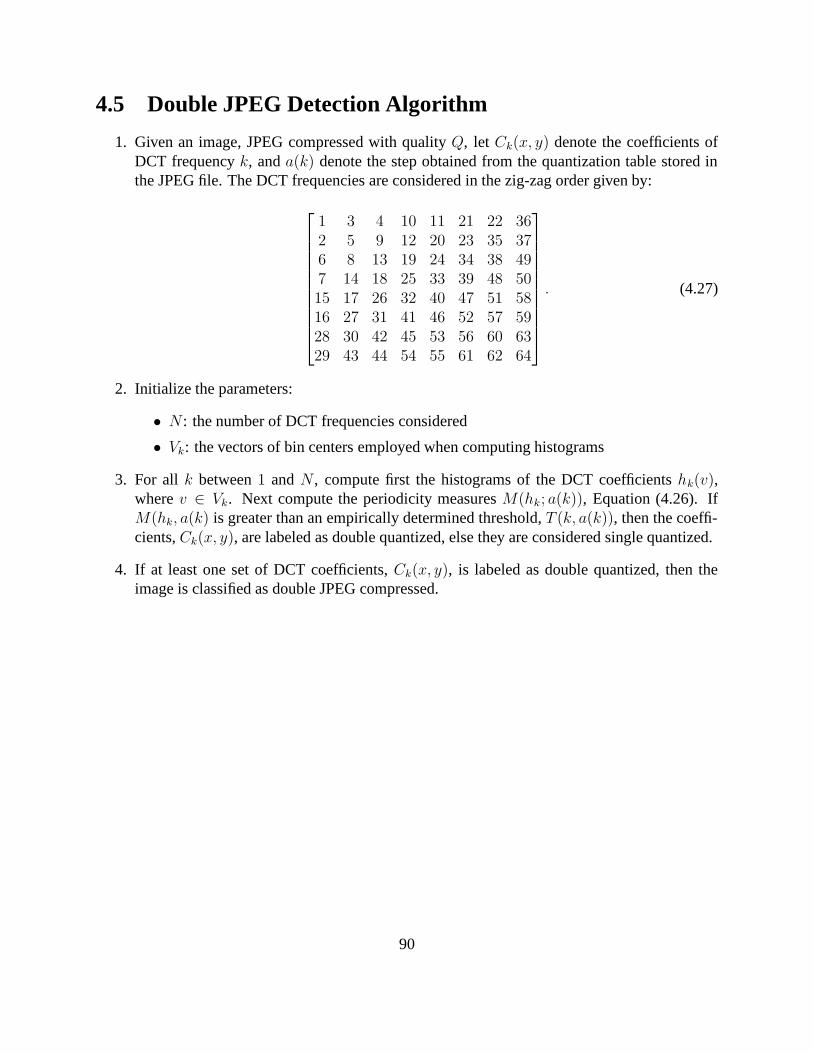
4.5 Double JPEG Detection Algorithm

1. Given an image, JPEG compressed with quality Q, let Ck(x, y) denote the coefficients ofDCT frequency k, and a(k) denote the step obtained from the quantization table stored inthe JPEG file. The DCT frequencies are considered in the zig-zag order given by:

1 3 4 10 11 21 22 362 5 9 12 20 23 35 376 8 13 19 24 34 38 497 14 18 25 33 39 48 5015 17 26 32 40 47 51 5816 27 31 41 46 52 57 5928 30 42 45 53 56 60 6329 43 44 54 55 61 62 64

. (4.27)

2. Initialize the parameters:

• N : the number of DCT frequencies considered

• Vk: the vectors of bin centers employed when computing histograms

3. For all k between 1 and N , compute first the histograms of the DCT coefficients hk(v),where v ∈ Vk. Next compute the periodicity measures M(hk; a(k)), Equation (4.26). IfM(hk, a(k) is greater than an empirically determined threshold, T (k, a(k)), then the coeffi-cients, Ck(x, y), are labeled as double quantized, else they are considered single quantized.

4. If at least one set of DCT coefficients, Ck(x, y), is labeled as double quantized, then theimage is classified as double JPEG compressed.

90

Chapter 5

Detection of Duplicated Image Regions

A common manipulation when tampering with an image is to copy and paste portions of the imageto conceal a person or object in the scene. If the splicing is imperceptible, little concern is typicallygiven to the fact that identical (or virtually identical) regions are present in the image. In thischapter, we present a technique that can efficiently detect and localize duplicated regions in animage. This technique works by first applying a principal component analysis (PCA) on smallfixed-size image blocks to yield a reduced dimension representation. This representation is robustto minor variations in the image due to additive noise or lossy compression. Duplicated regionsare then detected by lexicographically sorting all the image blocks. A similar method for detectingduplicated regions based on lexicographic sorting of DCT block coefficients was proposed in [24].While both methods employ a similar approach, the data-driven PCA basis may better capturediscriminating features. We show the efficacy of this technique on credible forgeries, and quantifyits robustness and sensitivity to additive noise, and lossy compression schemes.

5.1 Detecting Duplicated Regions

Given an image with N pixels our task is to determine if it contains duplicated regions of un-known location and shape. An exhaustive approach that examines every possible pair of regionshas an exponential complexity in the number of image pixels, and is obviously computationallyprohibitive. A more efficient algorithm might look for duplication of small fixed-sized blocks1.By stringing each such block into a vector and lexicographically sorting all image blocks, identicalblocks correspond to adjacent pairs in the sorted list. The primary cost of this algorithm is given bythe lexicographic sorting, yielding a complexity in O(N log N), since the number of image blocksis proportional to N , the number of image pixels. Note that this is a significant improvement overthe brute-force exponential algorithm. The drawback of this approach, however, is that it is sen-sitive to small variations between duplicated regions due to, for example, additive noise or lossycompression. We describe next an algorithm that overcomes these limitations while retaining itsefficiency.

1We assume that the size of the blocks is considerably smaller than the duplicated region to be detected.

91

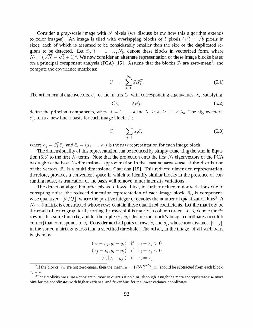
Consider a gray-scale image with N pixels (we discuss below how this algorithm extendsto color images). An image is tiled with overlapping blocks of b pixels (

√b ×

√b pixels in

size), each of which is assumed to be considerably smaller than the size of the duplicated re-gions to be detected. Let ~xi, i = 1, . . . , Nb, denote these blocks in vectorized form, whereNb = (

√N −

√b + 1)2. We now consider an alternate representation of these image blocks based

on a principal component analysis (PCA) [15]. Assume that the blocks ~xi are zero-mean2, andcompute the covariance matrix as:

C =

Nb∑

i=1

~xi~xTi . (5.1)

The orthonormal eigenvectors, ~ej , of the matrix C, with corresponding eigenvalues, λj , satisfying:

C~ej = λj~ej, (5.2)

define the principal components, where j = 1, . . . , b and λ1 ≥ λ2 ≥ · · · ≥ λb. The eigenvectors,~ej , form a new linear basis for each image block, ~xi:

~xi =b∑

j=1

aj~ej, (5.3)

where aj = ~xTi ~ej, and ~ai = (a1 . . . ab) is the new representation for each image block.

The dimensionality of this representation can be reduced by simply truncating the sum in Equa-tion (5.3) to the first Nt terms. Note that the projection onto the first Nt eigenvectors of the PCAbasis gives the best Nt-dimensional approximation in the least squares sense, if the distributionof the vectors, ~xi, is a multi-dimensional Gaussian [15]. This reduced dimension representation,therefore, provides a convenient space in which to identify similar blocks in the presence of cor-rupting noise, as truncation of the basis will remove minor intensity variations.

The detection algorithm proceeds as follows. First, to further reduce minor variations due tocorrupting noise, the reduced dimension representation of each image block, ~ai, is component-wise quantized, b~ai/Qc, where the positive integer Q denotes the number of quantization bins3. ANb × b matrix is constructed whose rows contain these quantized coefficients. Let the matrix S bethe result of lexicographically sorting the rows of this matrix in column order. Let ~si denote the ith

row of this sorted matrix, and let the tuple (xi, yi) denote the block’s image coordinates (top-leftcorner) that corresponds to ~si. Consider next all pairs of rows ~si and ~sj , whose row distance, |i−j|,in the sorted matrix S is less than a specified threshold. The offset, in the image, of all such pairsis given by:

(xi − xj, yi − yj) if xi − xj > 0

(xj − xi, yi − yj) if xi − xj < 0

(0, |yi − yj|) if xi = xj

2If the blocks, ~xi, are not zero-mean, then the mean, ~µ = 1/Nb

∑Nb

i=1 ~xi, should be subtracted from each block,~xi − ~µ.

3For simplicity we a use a constant number of quantization bins, although it might be more appropriate to use morebins for the coordinates with higher variance, and fewer bins for the lower variance coordinates.

92

From a list of all such offsets, duplicated regions in the image are detected by noting the offsetswith high occurrence. For example, a large duplicated region will consist of many smaller blocks,each of these blocks will appear in close proximity to each other in the lexicographically sortedmatrix, and will have the same offset. In order to avoid false hits due to uniform intensity areas,offset magnitudes below a specified threshold are ignored. See Section 5.4 for a detailed step-by-step algorithm.

The results of this detection can be visualized by constructing a duplication map — a zeroimage of the same size as the original is created, and all pixels in a region believed to be dupli-cated are assigned a unique gray-scale value. The complexity of this algorithm, dominated bythe lexicographic sorting, is in O(NtN log N), where Nt is the dimension of the PCA reducedrepresentations and N is the total number of image pixels.

There are at least two ways in which this algorithm can be extended to color images. Thesimplest approach is to independently process each color channel (e.g., RGB) to yield three dupli-cation maps. The second approach is to apply PCA to color blocks of size 3b, and proceed in thesame way as described above. The duplication detection algorithm can also be employed to detectif two, or more, images contain identical regions, as would happen when a region from one imageis copied then pasted into a different image. Given two images, the PCA is applied to overlappingblocks from both images, and the detection proceeds as in the single image case.

5.2 Results

Shown in Figures 5.1-5.3 are original and tampered images. The tampering consisted of copyingand pasting a region in the image to conceal a person or object. Shown in the lower portion ofthese figures are the outputs of our detection algorithm as applied to the tampered image saved withJPEG quality factors between 50 and 100. In each map, the two duplicated regions are shown withdifferent gray-scale values. In all of these examples, all parameters were fixed and set to: b = 64,ε = 0.01, Q = 256, Nn = 100, Nf = 128, Nd = 16 (see Section 5.4 for details). Truncation ofthe PCA basis typically reduces the dimension from 64 to 32. The average runtime for one colorchannel of a 512 × 512 image running on a 3 GHz processor, is approximately 10 seconds. Forvisualization purposes, the duplication map was (1) dilated then eroded to eliminate holes in theduplicated regions, and (2) eroded then dilated to eliminate spurious pairs of duplicated blocks. Adisk-shaped structuring element with a radius of 20 pixels was employed for these morphologicoperations [26].

To quantify the robustness and sensitivity of our algorithm we constructed a database of 100color images of size 512×512 pixels. These images were cropped from larger 2000×3008 imagestaken with a Nikon D100 digital camera. In each image, a random square region was copied andpasted onto a random, non-overlapping position in the image. Each image was then either JPEG orJPEG2000 compressed with varying quality factors, or corrupted with additive noise with varyingsignal to noise ratios (SNR). Shown on the top row of Figure 5.4, for example, are four images withduplicated regions of size 32 × 32, 64 × 64, 96 × 96, and 128 × 128 — the first two images werecompressed with JPEG qualities 85 and 65, and the other two images were corrupted with additive

93

original tampered

50 60 70

80 90 100

Figure 5.1: Shown are an original and a tampered image. Shown below are the output duplicationmaps from the green channel of the tampered image saved with JPEG qualities ranging between 50

and 100.

94

original tampered

50 60 70

80 90 100

50 60 70

80 90 100

Figure 5.2: Shown are an original and a tampered image. Shown below are the output duplicationmaps (corresponding to different regions used to conceal each person) from the green channel ofthe tampered image saved with JPEG qualities ranging between 50 and 100.

95

original tampered

50 60 70

80 90 100

Figure 5.3: Shown are an original and a tampered image. Shown below are the output duplicationmaps from the green channel of the tampered image saved with JPEG qualities ranging between 50

and 100.

96

JPEG (85) JPEG (65) SNR (36 db) SNR (29 db)

Figure 5.4: Shown on the top row are four images with duplicated regions of size 32 × 32, 64 × 64,96 × 96, and 128 × 128, after having been JPEG compressed (first and second images) or corruptedwith additive noise (third and fourth images). Shown below are the duplication maps returned whenrunning our algorithm on each image’s green channel.

noise with SNRs of 36db and 29db. Shown on the bottom row of Figure 5.4 are the duplicationmaps returned when running our algorithm on the green channel of each image. In these examples,and those described below, all parameters were set to: b = 64, ε = 0.01, Q = 256, Nn = 100,Nf = 128, Nd = 16. Shown in Figure 5.5 are the detection accuracy and the false positive rateas functions of JPEG compression quality for different sizes of duplicated regions. Note that theaccuracy is, in general, very good, except for small block sizes and low JPEG qualities. Note alsothat the average number of false positives (regions incorrectly labeled as duplicated) is relativelylow. Shown in Figure 5.6 are the detection accuracy and the false positive rate as functions ofthe JPEG2000 compression quality (in bits per pixel). The accuracy is nearly perfect for blocksizes greater than 32 × 32, and the false positive rate is low. When compared to classic JPEG,the only notable difference is that, in JPEG2000 compressed images, the detection of 64 × 64duplicated regions is more robust (higher accuracy for lower qualities), while the detection of32 × 32 duplicated regions is less robust (lower accuracy for higher qualities). Shown in Figure 5.7are the detection accuracy and false positive rate as functions of signal to noise ratio (SNR) ofadditive white Gaussian noise. As in the previous examples, the detection rates are nearly perfect,except for small block sizes and low SNR. Non-linear point-wise transformations, e.g., gammacorrection, do not affect the detection of duplicated regions in an image as long as they are applieduniformly across the image. The same is true for GIF compression. Since identical color pixelsin the original image map to the same indexed color in the GIF image, duplicated regions in theoriginal image remain identical in the GIF image.

97

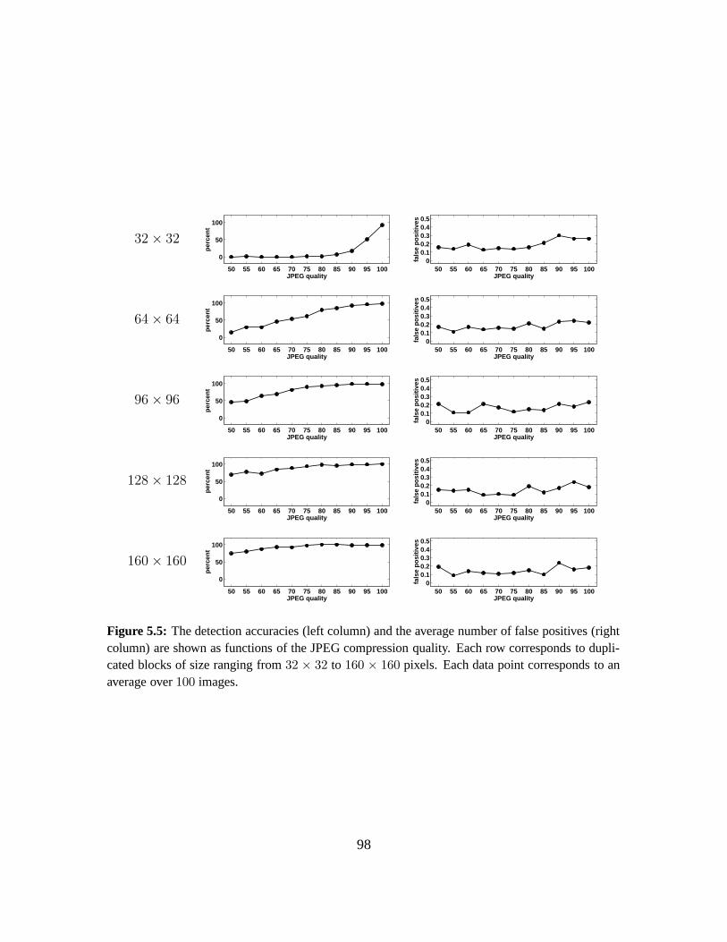
32 × 32

50 55 60 65 70 75 80 85 90 95 100

0

50

100

JPEG quality

per

cen

t

50 55 60 65 70 75 80 85 90 95 1000

0.10.20.30.40.5

JPEG quality

fals

e p

osi

tive

s

64 × 64

50 55 60 65 70 75 80 85 90 95 100

0

50

100

JPEG quality

per

cen

t

50 55 60 65 70 75 80 85 90 95 1000

0.10.20.30.40.5

JPEG quality

fals

e p

osi

tive

s

96 × 96

50 55 60 65 70 75 80 85 90 95 100

0

50

100

JPEG quality

per

cen

t

50 55 60 65 70 75 80 85 90 95 1000

0.10.20.30.40.5

JPEG quality

fals

e p

osi

tive

s

128 × 128

50 55 60 65 70 75 80 85 90 95 100

0

50

100

JPEG quality

per

cen

t

50 55 60 65 70 75 80 85 90 95 1000

0.10.20.30.40.5

JPEG quality

fals

e p

osi

tive

s

160 × 160

50 55 60 65 70 75 80 85 90 95 100

0

50

100

JPEG quality

per

cen

t

50 55 60 65 70 75 80 85 90 95 1000

0.10.20.30.40.5

JPEG quality

fals

e p

osi

tive

s

Figure 5.5: The detection accuracies (left column) and the average number of false positives (rightcolumn) are shown as functions of the JPEG compression quality. Each row corresponds to dupli-cated blocks of size ranging from 32 × 32 to 160 × 160 pixels. Each data point corresponds to anaverage over 100 images.

98

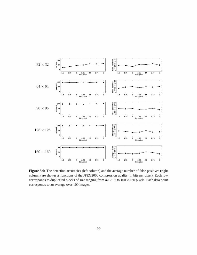
32 × 32

1.5 1.75 2 2.25 2.5 2.75 3

0

50

100

bits/pixel

per

cen

t

1.5 1.75 2 2.25 2.5 2.75 30

0.10.20.30.40.5

bits/pixel

fals

e p

osi

tive

s

64 × 64

1.5 1.75 2 2.25 2.5 2.75 3

0

50

100

bits/pixel

per

cen

t

1.5 1.75 2 2.25 2.5 2.75 30

0.10.20.30.40.5

bits/pixel

fals

e p

osi

tive

s

96 × 96

1.5 1.75 2 2.25 2.5 2.75 3

0

50

100

bits/pixel

per

cen

t

1.5 1.75 2 2.25 2.5 2.75 30

0.10.20.30.40.5

bits/pixel

fals

e p

osi

tive

s

128 × 128

1.5 1.75 2 2.25 2.5 2.75 3

0

50

100

bits/pixel

per

cen

t

1.5 1.75 2 2.25 2.5 2.75 30

0.10.20.30.40.5

bits/pixel

fals

e p

osi

tive

s

160 × 160

1.5 1.75 2 2.25 2.5 2.75 3

0

50

100

bits/pixel

per

cen

t

1.5 1.75 2 2.25 2.5 2.75 30

0.10.20.30.40.5

bits/pixel

fals

e p

osi

tive

s

Figure 5.6: The detection accuracies (left column) and the average number of false positives (rightcolumn) are shown as functions of the JPEG2000 compression quality (in bits per pixel). Each rowcorresponds to duplicated blocks of size ranging from 32× 32 to 160× 160 pixels. Each data pointcorresponds to an average over 100 images.

99

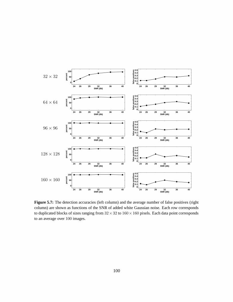
32 × 32

24 26 29 32 36 40

0

50

100

SNR (db)

per

cen

t

24 26 29 32 36 400

0.10.20.30.40.5

SNR (db)

fals

e p

osi

tive

s

64 × 64

24 26 29 32 36 40

0

50

100

SNR (db)

per

cen

t

24 26 29 32 36 400

0.10.20.30.40.5

SNR (db)

fals

e p

osi

tive

s

96 × 96

24 26 29 32 36 40

0

50

100

SNR (db)

per

cen

t

24 26 29 32 36 400

0.10.20.30.40.5

SNR (db)

fals

e p

osi

tive

s

128 × 128

24 26 29 32 36 40

0

50

100

SNR (db)

per

cen

t

24 26 29 32 36 400

0.10.20.30.40.5

SNR (db)

fals

e p

osi

tive

s

160 × 160

24 26 29 32 36 40

0

50

100

SNR (db)

per

cen

t

24 26 29 32 36 400

0.10.20.30.40.5

SNR (db)

fals

e p

osi

tive

s

Figure 5.7: The detection accuracies (left column) and the average number of false positives (rightcolumn) are shown as functions of the SNR of added white Gaussian noise. Each row correspondsto duplicated blocks of sizes ranging from 32×32 to 160×160 pixels. Each data point correspondsto an average over 100 images.

100

5.3 Summary

We have presented an efficient and robust technique that automatically detects duplicated regionsin an image. This technique works by first applying a principal component analysis (PCA) onsmall, fixed-size image blocks to yield a reduced dimension representation that is robust to minorvariations in the image due to additive noise or lossy compression. Duplicated regions are thendetected by lexicographically sorting all the image blocks. We have shown the effectiveness ofthis technique on plausible forgeries, and have quantified its sensitivity to additive noise, and lossycompression schemes — we find that detection is possible even in the presence of significantamounts of distortion.

101

5.4 Duplication Detection Algorithm

1. Let N be the total number of pixels in a gray-scale or color image

2. Initialize the parameters:

• b: number of pixels per block (√

b ×√

b pixels in dimension) — there areNb = (

√N −

√b + 1)2 such blocks

• ε: fraction of the ignored variance along the principal axes

• Q: number of quantization bins

• Nn: number of neighboring rows to search in lexicographically sorted matrix

• Nf : minimum frequency threshold

• Nd: minimum offset threshold

3. Using PCA, compute the new Nt-dimensional representation, ~ai, i = 1, . . . , Nb, of each bpixel image block (for color images: (1) analyze each color channel separately; or (2) build

a single color block of size 3b pixels). The value of Nt is chosen to satisfy: 1 − ε =PNt

i=1λi

Pbi=1

λi,

where λi are the eigenvalues as computed by the PCA, Equation (5.2).

4. Build a Nb × b matrix whose rows are given by the component-wise quantized coordinates:b~ai/Qc.

5. Sort the rows of the above matrix in lexicographic order to yield a matrix S. Let ~si denotethe rows of S, and let (xi, yi) denote the coordinates (top-left corner in the image) of theblock that corresponds to ~si.

6. For every pair of rows ~si and ~sj from S such that |i − j| < Nn, place the pair of coordinates(xi, yi) and (xj, yj) onto a list.

7. For all elements in this list, compute their offsets, defined as:

(xi − xj, yi − yj) if xi − xj > 0

(xj − xi, yi − yj) if xi − xj < 0

(0, |yi − yj|) if xi = xj

8. Discard all pairs of coordinates with an offset frequency less than Nf .

9. Discard all pairs whose offset magnitude,√

(xi − xj)2 + (yi − yj)2, is less than Nd.

10. From the remaining pairs of blocks build a duplication map by constructing a zero imageof the same size as the original, and coloring all pixels in a duplicated region with a uniquegray-scale intensity value.

102

Chapter 6

Blind Estimation of Background Noise

Digital images have an inherent amount of noise introduced either by the imaging process or bydigital compression. The amount of noise is typically uniform across the entire image. If twoimages with different noise levels are spliced together, or if small amounts of noise are locallyadded to conceal traces of tampering, then variations in the local noise variance across the imagecan be used as evidence of tampering. Measuring the local noise variance is non-trivial in theabsence of the original signal. Several blind signal to noise ratio (SNR) estimators have, however,been proposed [49]. Since these estimators work by estimating the variances of both the signaland the noise, they can be employed to measure the local noise variance of an image1. We presentone such estimator, M2M4 [43], and show its effectiveness in measuring the local noise variancein images.

6.1 Blind Signal-to-Noise Ratio Estimation

We begin by assuming an additive noise model:

y[t] = x[t] + w[t], (6.1)

where x[t] is the uncorrupted signal with variance S and w[t] is the noise with variance N . LetM2 = E {y2[t]} and M4 = E {y4[t]} denote the second and forth moments of the corrupted signal,where E {·} is the expected value operator2. Assuming that the signal and noise are independent

1To be invariant to the underlying signal strength, we analyze the noise variance instead of the ratio of signal tonoise variances.

2In practice, all the expected values are estimated as sample averages. For example, the second and forthmoments of the noisy signal are computed as: M2 = 1

N

∑N

t=1(y[t] − µ)2, and M4 = 1N

∑N

t=1(y[t] − µ)4, where

µ = 1N

∑N

t=1 y[t] denotes the sample mean.

103

and zero-mean, it was shown [49] that M2 and M4 take the form:

M2 = E{

y2[t]}

= E{

(x[t] + w[t])2}

= E{

x2[t]}

+ 2 E {x[t]w[t]} + E{

w2[t]}

= S + N (6.2)

M4 = E{

y4[t]}

= E{

(x[t] + w[t])4}

= E{

x4[t]}

+ 4 E{

x3[t]w[t]}

+ 6 E{

x2[t]w2[t]}

+ 4 E{

x[t]w3[t]}

+ E{

w4[t]}

= kxS2 + 6SN + kwN2, (6.3)

where kx = E {x4[t]} /(E {x2[t]})2 and kw = E {w4[t]} /(E {w2[t]})2 are the kurtosis’s values ofthe original signal and noise. Solving Equations (6.2-6.3) for S and N yields the estimators:

S =M2(kw − 3) ±

√

(9 − kxkw)M22 + M4(kx + kw − 6)

kx + ky − 6(6.4)

N = M2 − S. (6.5)

Assuming white Gaussian noise (kw = 3), and denoting the kurtosis of the noisy signal withky = M4/M

22 , the Equations (6.4-6.5) become:

S = M2

√

ky − 3

kx − 3(6.6)

N = M2

(

1 −√

ky − 3

kx − 3

)

. (6.7)

Note that these estimators work only when the original signal is not Gaussian, i.e., kx 6= 3. Notealso that in order to obtain reasonable estimates from Equations (6.6-6.7), i.e., positive real values,the following condition must hold:

0 ≤ ky − 3

kx − 3≤ 1. (6.8)

This condition is equivalent to saying that the kurtosis of the noisy signal, ky must be between thekurtosis of the original signal, kx, and three, the kurtosis of the noise. Due to numerical errorsand to the fact that instead of the true kurtosis values, sample average estimators are employed,the above conditions may not be always fulfilled, and complex or negative values may occur onoccasion.

Note that for these estimators the kurtosis of the original signal is assumed to be known, whichmay not be true in general. In the results presented below, it is assumed to be known. It may bepossible, for example, to estimate the original kurtosis from a region of an image that is believedto be unadulterated.

104

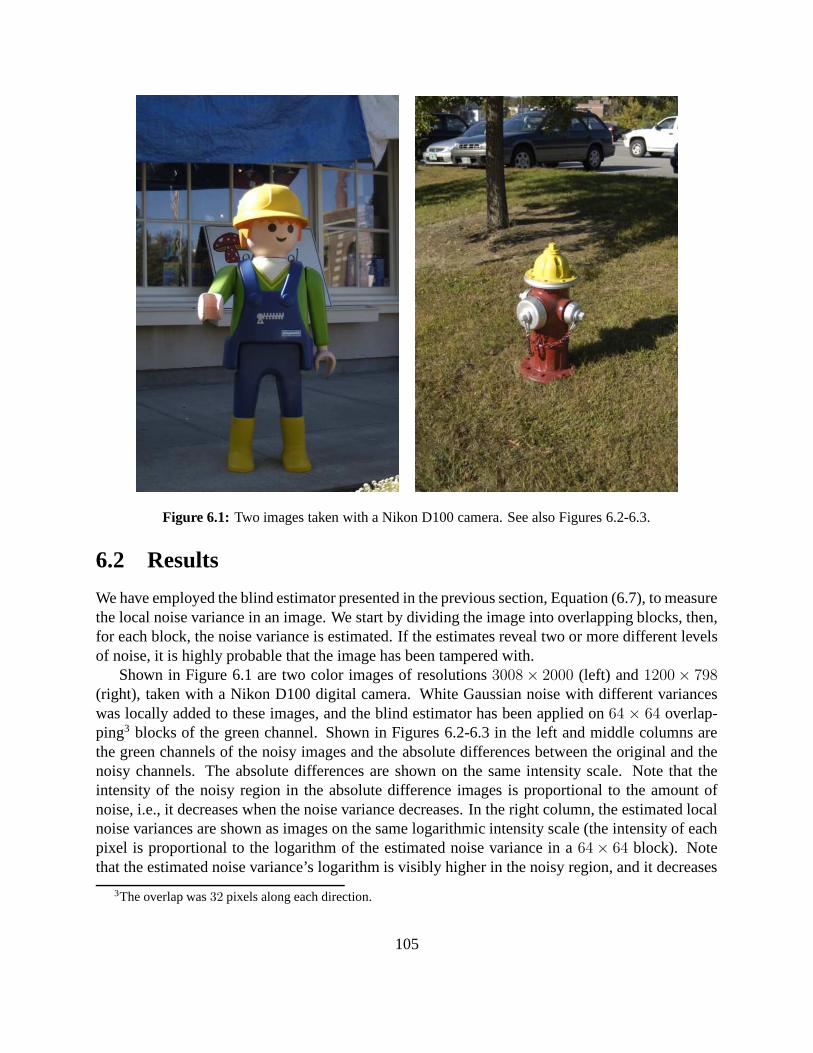
Figure 6.1: Two images taken with a Nikon D100 camera. See also Figures 6.2-6.3.

6.2 Results

We have employed the blind estimator presented in the previous section, Equation (6.7), to measurethe local noise variance in an image. We start by dividing the image into overlapping blocks, then,for each block, the noise variance is estimated. If the estimates reveal two or more different levelsof noise, it is highly probable that the image has been tampered with.

Shown in Figure 6.1 are two color images of resolutions 3008 × 2000 (left) and 1200 × 798(right), taken with a Nikon D100 digital camera. White Gaussian noise with different varianceswas locally added to these images, and the blind estimator has been applied on 64 × 64 overlap-ping3 blocks of the green channel. Shown in Figures 6.2-6.3 in the left and middle columns arethe green channels of the noisy images and the absolute differences between the original and thenoisy channels. The absolute differences are shown on the same intensity scale. Note that theintensity of the noisy region in the absolute difference images is proportional to the amount ofnoise, i.e., it decreases when the noise variance decreases. In the right column, the estimated localnoise variances are shown as images on the same logarithmic intensity scale (the intensity of eachpixel is proportional to the logarithm of the estimated noise variance in a 64 × 64 block). Notethat the estimated noise variance’s logarithm is visibly higher in the noisy region, and it decreases

3The overlap was 32 pixels along each direction.

105

32 × 32 64 × 64

actual estimated (db)(db) mean std min max-6.00 -6.045 0.255 -6.535 -5.411-5.50 -5.608 0.227 -6.018 -5.018-5.00 -5.138 0.179 -5.428 -4.675-4.50 -4.617 0.127 -4.805 -4.259-4.00 -4.059 0.079 -4.205 -3.846-3.50 -3.490 0.049 -3.612 -3.390-3.00 -2.947 0.040 -3.077 -2.862-2.50 -2.465 0.051 -2.606 -2.331-2.00 -2.083 0.076 -2.263 -1.884


96 × 96 128 × 128



Table 6.1: Shown are the statistics of the estimated noise variances (mean, standard deviation, andminimum and maximum values) as obtained for different block sizes. These statistics have beenobtained from 50 natural images. On average, the correct value is estimated with 1.5% of the actualvalue. See also Figure 6.4.

proportionally with the amount of noise.


To quantify the sensitivity of the blind noise variance estimation, we have employed a database of100 color images 1024 × 1024 in size. These images were cropped from a smaller set of 30 images3008 × 2000 pixels in size, taken with a Nikon D100 camera.

Single-Channel Gray-Scale Images

We have employed the green channels of the images in our database as single-channel, gray-scaleimages. White Gaussian noise with different variances was uniformly added to these gray-scaleimages. Each image was divided into overlapping blocks (with an overlap of 50% of the block size

106

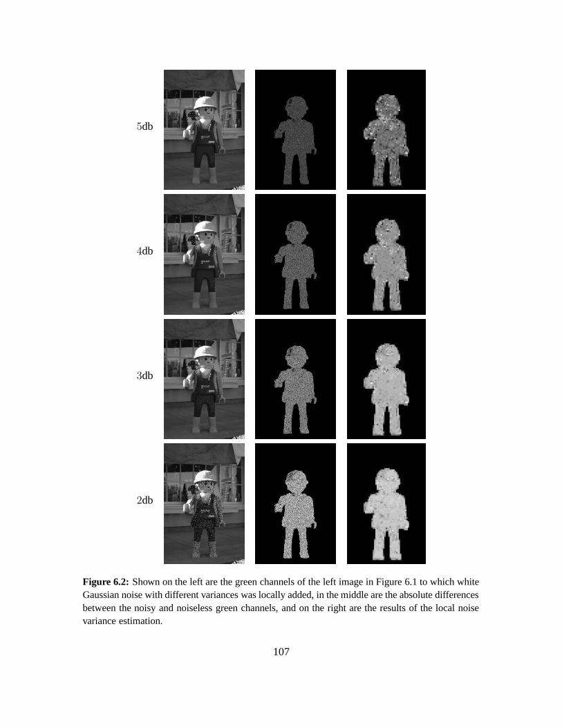
5db

4db

3db

2db

Figure 6.2: Shown on the left are the green channels of the left image in Figure 6.1 to which whiteGaussian noise with different variances was locally added, in the middle are the absolute differencesbetween the noisy and noiseless green channels, and on the right are the results of the local noisevariance estimation.

107

5db

4db

3db

2db

Figure 6.3: Shown on the left are the green channels of the right image in Figure 6.1 to which whiteGaussian noise with different variances was locally added, in the middle are the absolute differencesbetween the noisy and noiseless green channels, and on the right are the results of the local noisevariance estimation.

108

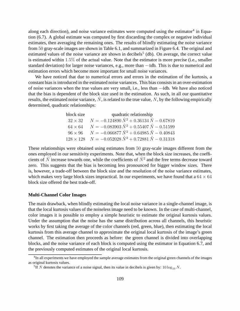
along each direction), and noise variance estimates were computed using the estimator4 in Equa-tion (6.7). A global estimate was computed by first discarding the complex or negative individualestimates, then averaging the remaining ones. The results of blindly estimating the noise variancefrom 50 gray-scale images are shown in Table 6.1, and summarized in Figure 6.4. The original andestimated values of the noise variance are shown in decibels5 (db). On average, the correct valueis estimated within 1.5% of the actual value. Note that the estimator is more precise (i.e., smallerstandard deviation) for larger noise variances, e.g., more than −4db. This is due to numerical andestimation errors which become more important for small noise variances.

We have noticed that due to numerical errors and errors in the estimation of the kurtosis, aconstant bias is introduced in the estimated noise variances. This bias consists in an over-estimationof noise variances when the true values are very small, i.e., less than −4db. We have also noticedthat the bias is dependent of the block size used in the estimation. As such, in all our quantitativeresults, the estimated noise variance, N , is related to the true value, N , by the following empiricallydetermined, quadratic relationships:

block size quadratic relationship32 × 32 N = −0.124890 N2 + 0.36134 N − 0.67819

64 × 64 N = −0.083903 N2 + 0.55407 N − 0.51599

96 × 96 N = −0.066877 N2 + 0.64985 N − 0.40843

128 × 128 N = −0.052028 N2 + 0.72881 N − 0.31318

These relationships were obtained using estimates from 50 gray-scale images different from theones employed in our sensitivity experiments. Note that, when the block size increases, the coeffi-cients of N increase towards one, while the coefficients of N2 and the free terms decrease towardzero. This suggests that the bias is becoming less pronounced for bigger window sizes. Thereis, however, a trade-off between the block size and the resolution of the noise variance estimates,which makes very large block sizes impractical. In our experiments, we have found that a 64 × 64block size offered the best trade-off.

Multi-Channel Color Images

The main drawback, when blindly estimating the local noise variance in a single-channel image, isthat the local kurtosis values of the noiseless image need to be known. In the case of multi-channel,color images it is possible to employ a simple heuristic to estimate the original kurtosis values.Under the assumption that the noise has the same distribution across all channels, this heuristicworks by first taking the average of the color channels (red, green, blue), then estimating the localkurtosis from this average channel to approximate the original local kurtosis of the image’s greenchannel. The estimation then proceeds as before: the green channel is divided into overlappingblocks, and the noise variance of each block is computed using the estimator in Equation 6.7, andthe previously computed estimates of the original local kurtosis.

4In all experiments we have employed the sample average estimates from the original green channels of the imagesas original kurtosis values.

5If N denotes the variance of a noise signal, then its value in decibels is given by: 10 log10 N .

109

32 × 32 64 × 64

−6 −5.5 −5 −4.5 −4 −3.5 −3 −2.5 −2

−6

−5.5

−5

−4.5

−4

−3.5

−3

−2.5

−2

actual noise variance (db)

estim

ated

noi

se v

aria

nce

(db)

−6 −5.5 −5 −4.5 −4 −3.5 −3 −2.5 −2

−6

−5.5

−5

−4.5

−4

−3.5

−3

−2.5

−2


estim

ated

noi

se v

aria

nce

(db)

96 × 96 128 × 128

−6 −5.5 −5 −4.5 −4 −3.5 −3 −2.5 −2

−6

−5.5

−5

−4.5

−4

−3.5

−3

−2.5

−2


estim

ated

noi

se v

aria

nce

(db)

−6 −5.5 −5 −4.5 −4 −3.5 −3 −2.5 −2

−6

−5.5

−5

−4.5

−4

−3.5

−3

−2.5

−2


estim

ated

noi

se v

aria

nce

(db)

Figure 6.4: Shown are the average estimated noise variances and their standard deviations, plottedagainst the true values of the noise variances. Each data point corresponds to an average over 50

images using blocks of various sizes. See also Table 6.1.

110

White Gaussian noise with different variances was uniformly added to the color images inthe database. For a given color image, the variance of the noise was the same for each channel.The results of blindly estimating the local noise variance from 50 color images (when the aboveheuristic is employed) are shown in Table 6.2, and summarized in Figure 6.5. The original andestimated noise variances are shown in decibels (db). Note that, for noise variances greater than−3db, the estimation is both accurate and precise, that is, the mean of the estimates is close to theactual value, and the standard deviation of the estimates is small. For noise variances smaller than−4db, however, the estimation fails. The reason for this poor performance is related to both thefailure of our heuristic to accurately estimate the original local kurtosis, and to the errors in theother sample average estimates.

As in the experiments with single-channel images, we have noticed that due to numerical andsample average errors, a constant bias is introduced in the estimated noise variances. We haveempirically found that a linear model suffices to approximate this bias well. We have employed theaverage estimates in the range between −3.5db and −1db (i.e., the range for which the discrimina-tion of different noise levels is possible), to empirically estimate linear relationships between theestimated and true noise variances:

block size linear relationship32 × 32 N = 1.2572 N − 0.91292

64 × 64 N = 1.2947 N − 0.87348

96 × 96 N = 1.2957 N − 0.85403

128 × 128 N = 1.2894 N − 0.82960

These relationships were obtained using estimates from 50 color images different from the onesemployed in the sensitivity experiments above. Note that the parameters of these linear relation-ships are practically independent of the window size used in the estimation.

6.3 Summary

We have presented a technique for blindly estimating local noise variance and showed how it can beapplied to detect the presence of multiple levels of noise in an image. This technique assumes thatthe kurtosis of local patches of the original image is known, and that the noise is white, Gaussian,and statistically independent of the original image. The estimation method can be adapted to dealwith different types of noise with known statistical properties (i.e., the kurtosis). We have shownthe efficacy of measuring the local noise variance in natural images with locally added noise, andwe have quantified the sensitivity of the estimation method.

111

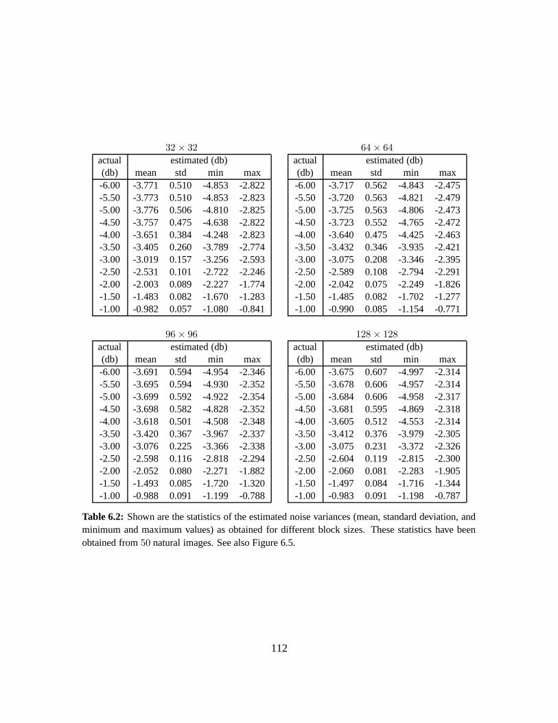
32 × 32 64 × 64

actual estimated (db)(db) mean std min max-6.00 -3.771 0.510 -4.853 -2.822-5.50 -3.773 0.510 -4.853 -2.823-5.00 -3.776 0.506 -4.810 -2.825-4.50 -3.757 0.475 -4.638 -2.822-4.00 -3.651 0.384 -4.248 -2.823-3.50 -3.405 0.260 -3.789 -2.774-3.00 -3.019 0.157 -3.256 -2.593-2.50 -2.531 0.101 -2.722 -2.246-2.00 -2.003 0.089 -2.227 -1.774-1.50 -1.483 0.082 -1.670 -1.283-1.00 -0.982 0.057 -1.080 -0.841


96 × 96 128 × 128



Table 6.2: Shown are the statistics of the estimated noise variances (mean, standard deviation, andminimum and maximum values) as obtained for different block sizes. These statistics have beenobtained from 50 natural images. See also Figure 6.5.

112

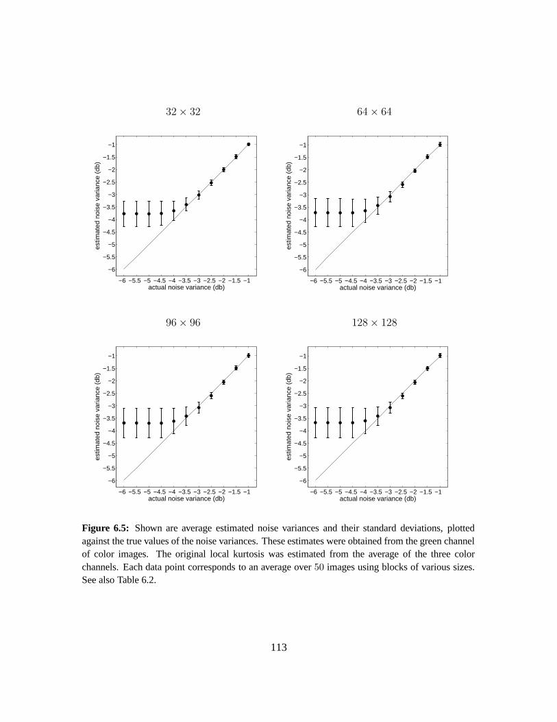
32 × 32 64 × 64

−6 −5.5 −5 −4.5 −4 −3.5 −3 −2.5 −2 −1.5 −1

−6

−5.5

−5

−4.5

−4

−3.5

−3

−2.5

−2

−1.5

−1


estim

ated

noi

se v

aria

nce

(db)

−6 −5.5 −5 −4.5 −4 −3.5 −3 −2.5 −2 −1.5 −1

−6

−5.5

−5

−4.5

−4

−3.5

−3

−2.5

−2

−1.5

−1

actual noise variance (db)es

timat

ed n

oise

var

ianc

e (d

b)

96 × 96 128 × 128

−6 −5.5 −5 −4.5 −4 −3.5 −3 −2.5 −2 −1.5 −1

−6

−5.5

−5

−4.5

−4

−3.5

−3

−2.5

−2

−1.5

−1


estim

ated

noi

se v

aria

nce

(db)

−6 −5.5 −5 −4.5 −4 −3.5 −3 −2.5 −2 −1.5 −1

−6

−5.5

−5

−4.5

−4

−3.5

−3

−2.5

−2

−1.5

−1


estim

ated

noi

se v

aria

nce

(db)

Figure 6.5: Shown are average estimated noise variances and their standard deviations, plottedagainst the true values of the noise variances. These estimates were obtained from the green channelof color images. The original local kurtosis was estimated from the average of the three colorchannels. Each data point corresponds to an average over 50 images using blocks of various sizes.See also Table 6.2.

113

Chapter 7

Conclusion

In the previous chapters, we have presented five techniques for detecting different forms of tam-pering in manipulated digital images: (1) traces of re-sampling [52] (e.g., scaling, rotation); (2)manipulations of color filter array interpolated images [53]; (3) double JPEG compression [51];(4) duplicated regions [50]; and (5) inconsistent noise patterns [51]. Although these techniques aredifferent, they work in a common framework under the assumption that tampering may alter someunderlying statistical properties of natural images. For each technique, the general approach hasbeen the same: first, statistical changes associated with specific types of tampering are identifiedand quantified, then detection methods are designed to estimate these changes and differentiatebetween tampered and unadulterated images.

When digitally compositing two, or more, images, it is often necessary to scale, rotate, orstretch the original images, or portions of them, in order to create a convincing match. Thesemanipulations require re-sampling the original images onto a different sampling lattice. We haveshown, Chapter 2, that re-sampling introduces specific correlations between neighboring imagepixels. These correlations were quantified, and the expectation/maximization (EM) algorithm wasemployed to detect them in any portion of an image. This detection method can detect a broadrange of re-sampling parameters, and is fairly robust to simple attacks. Experiments with lossycompressed images, however, have revealed a significant weakness in our technique: while rea-sonably robust on GIF and JPEG2000 images, our method is particularly sensitive to JPEG com-pression. This is because JPEG compression introduces a significant amount of band-pass noise,and specific artifacts that interfere with the detection of re-sampling correlations. We believe, how-ever, that our technique may still prove useful for a number of different forensic applications: forexample, a court of law may accept into evidence only JPEG images with minimal compression.

The re-sampling detection technique can also be employed to foil attacks on authenticationwatermarking schemes. Temporal and geometric distortions are a well-known class of attacks towhich robust watermarking schemes are particularly sensitive. In audio signals, temporal scalingcan occur from speed changes of a tape player, or can be the result of a sophisticated processdesigned to change the duration of sounds without altering the wavelengths of their spectra. Indigital photographs, geometric distortions can be the result of manipulations with a photo-editingsoftware. In video signals, both temporal and geometric distortions can occur when converting

114

between different encoding formats. These temporal and geometric distortions can be modeledwith an affine transformation. More specifically, a watermarked signal is first affine transformed,then re-sampled onto a different sampling lattice to yield a new signal in which the embeddedwatermark becomes unrecognizable by the watermark detector. To foil this attack, the distortionparameters are first blindly estimated using our re-sampling detection technique1, then the temporalor geometric distortions are inverted, and the embedded watermark recovered.

To capture color images, most digital cameras employ a single CCD or CMOS sensor in con-junction with a color filter array (CFA). At each pixel location, a single color sample (out of three)is recorded, and the missing color samples are interpolated from neighboring samples. We haveshown, Chapter 3, that this process, referred to as CFA interpolation or demosaicking, introducesspecific correlations between neighboring color samples, similar to those present in re-sampledimages. A broad class of tampering techniques (e.g., re-touching, enhancing) are likely to destroyor significantly alter these correlations. As such, the presence, absence, or distortion of CFA in-terpolation correlations may represent evidence of authenticity or tampering. We have quantifiedthese correlations with a simple linear model, and employed the expectation/maximization (EM)algorithm to reveal their presence, or absence, in any portion of a CFA interpolated color image.We have tested our technique on images CFA interpolated with seven different schemes, and foundthat we can detect traces of tampering even in lossy compressed images. Although our methodis quite robust to simple counter attacks, we have found a vulnerability. If a tampered image isre-sampled onto a virtual CFA, then re-interpolated, the traces of tampering become undetectable.This attack, however, requires knowledge of the camera’s CFA pattern and interpolation scheme,and is not likely to be available to an average user. Another potential issue with this detectionmethod is the release of a new type of CMOS sensor, the Foveon X3, that can simultaneouslysample the three color channels at each pixel location. Images from cameras equipped with thissensor will no longer contain the CFA interpolation correlations employed to detect tampering.We believe, however, that our detection technique may still be useful given that traditional singlesensor cameras are likely to remain cheaper and more available to casual users.

A photo-editing software package (e.g., Adobe Photoshopr) is usually employed to manipulatedigital images. An image is first loaded into the photo-editing software, some manipulations areperformed, then it is re-saved. If the original and tampered images are stored in JPEG format,the default option for most digital cameras, then the tampered image has been double compressed.We have shown, Chapter 4, that when an image is double JPEG compressed specific correlationsare introduced between discrete cosine transform (DCT) coefficients of image blocks. We havequantified these correlations, and devised an algorithm that can distinguish between single anddouble JPEG compressed images. Although there are certain theoretical limitations that makedouble compressed images undetectable in some cases, we have tested our detection method on alarge number of images and found that double JPEG compression is detectable for a broad range ofquality factors. We have also found that our detection method is vulnerable to attack: if a tamperedJPEG image is cropped prior to re-saving, the correlations described in Chapter 4 are no longer

1It is possible that more than one set of distortion parameters are obtained from our detection method, e.g., imagerotations by angles θ◦ and −θ◦ are indistinguishable. In this case, the signal must be inverted with each possible setof distortion parameters, and the watermark detector must be applied to each inverted signal.

115

introduced. It is possible that other artifacts may be present, and this will be an interesting problemfor further research. Note that a double JPEG compressed image is not necessarily a forgery:for example, a user may re-save JPEG images with a lower quality to save storage space. Theauthenticity of a double JPEG compressed image, however, is questionable and further analysismay be required.

When trying to conceal a person or object in a digital image, a common manipulation is to copya portion of the same image, then paste it over the desired region. If the splicing is imperceptiblelittle concern is given to the fact that identical (or virtually identical) regions are present. An ex-haustive approach to detecting duplicated image regions is computationally prohibitive — it has anexponential complexity in the number of image pixels. We have proposed an efficient technique,Chapter 5, that can detect and localize duplicated regions in an image. The basic approach worksby first applying a principal component analysis (PCA) on small, fixed-size image blocks to yield areduced-dimensional representation robust to noise and lossy compression. Duplicated regions aredetected by lexicographically sorting the transformed image blocks, then examining pairs of neigh-boring blocks. We have shown the efficacy of this technique on credible forgeries, and analyzedits sensitivity to simple attacks and lossy compression. We have found that duplicated regions ofrelatively small size (e.g., 32×32 pixels) are harder to detect, particularly in the presence of noise.Note that this method requires human intervention to validate the potential duplicated regions re-turned by our algorithm. This is because fairly large regions with little variation (e.g., sky, asphaltroads) present in natural images tend to yield false positives, i.e., regions that are similar, but notduplicated. In our experiments, we have found that our algorithm yields a relatively low averagenumber of false positives, i.e., less than one percent. Our technique can also be employed to detectthe presence of duplicated regions in two, or more, different images, as might occur when a com-posite image is created by splicing together portions of several images. The principal componentanalysis is applied to fixed-size blocks from all images, then the algorithm proceeds as in the singleimage case.

Digital cameras introduce an inherent amount of noise uniformly spread across an image.When creating digital forgeries, it is common to add a small amount of additive noise to con-ceal traces of tampering, e.g., to obscure details in the background or at a splice boundary. As aresult, tampered images may contain inconsistent noise patterns, i.e., significant variations in thelocal noise variance. Measuring the noise variance in the absence of the original, noiseless image isa non-trivial, ill-defined problem. We have employed a blind signal to noise ratio (SNR) estimator,Chapter 6, to locally estimate the noise variance in an image and reveal the presence of inconsistentnoise levels. This estimator works under the assumption that the image and the noise are statisti-cally independent, and requires knowledge of the kurtosis values of local image patches, and thekurtosis of the noise. While the kurtosis of the noise may be known (e.g., it is equal to 3 for whiteGaussian noise) or easily estimated, reliably estimating the kurtosis of the original image patchesremains an open problem. Assuming, for gray-scale images, that the original values of the localkurtosis are known, and, for color images, employing a simple heuristic to estimate them, we haveillustrated how blind estimation of the local noise variance can reveal the presence of inconsistentnoise levels (a sign of tampering) in images with locally added noise. We have found, however,that due to numerical errors, and to errors in the sample average estimates of the kurtosis, a bias

116

is introduced in the estimation of the local noise variance. This bias was quantified, then removedfrom the estimation. Sensitivity experiments have shown that, in general, the estimation is fairlyaccurate. Not unexpectedly, we have noticed that due to numerical errors the estimation becomesless accurate for very small noise variances.

As with any authentication schemes, our statistical techniques may be vulnerable to counter-attack. Extensive experiments have shown that our algorithms are reasonably robust to simple at-tacks, e.g., lossy compression schemes, additive noise, and non-linear luminance transformations.We have, however, identified several more sophisticated attacks to which some of our detectionschemes are vulnerable. For example, re-sampling detection is particularly sensitive to lossy JPEGcompression, the correlations specific to color filter array interpolation can be simulated if thecolor pattern and interpolation scheme are known, and double quantization artifacts are no longerintroduced in a double JPEG compressed image, if the image is cropped prior to the second com-pression. In a forensic context, it is important that the development of authentication tools andthe analysis of their limitations go in parallel. A full analysis of these, and other, potential vul-nerabilities is beyond the scope of this thesis, and represents an interesting direction for futureresearch.

Most techniques proposed in this thesis were targeted towards detecting tampering in uncom-pressed or lossless compressed images. We have noticed that lossy compression schemes (e.g.,JPEG) introduce specific artifacts that interfere with some of our statistical methods. Since lossycompressed images are more widespread than their uncompressed counterparts (a significant pro-portion of digital cameras store images only in JPEG format) an important direction for futureresearch would be to design detection techniques targeted towards lossy compressed images.

Another interesting future research topic would be to investigate statistical techniques for de-tecting tampering in digitally scanned images. For example, color images captured with singlesensor cameras contain correlations specific to color filter array interpolation that can be employedfor image authentication. It may be worth investigating if similar correlations are introduced bydigital scanners, and if digitally scanned images and digital camera images have different statisticalproperties. This may also help foil the analog to digital attack in which a digital image is printed,then scanned in order to destroy embedded watermarks, or to conceal traces of tampering.

With the advent of low-cost, powerful computers and sophisticated editing tools even casualusers can manipulate digital video with relative ease. The resulting tampered video sequences canbe very hard to distinguish from authentic footage. It is likely, however, that tampering might altersome underlying statistical properties of natural video sequences. A future research topic would beto investigate what statistical changes occur when tampering with video sequences, and to designdetection techniques that quantify and estimate these changes. A potential issue is that most digitalvideo sequences are encoded with lossy compression techniques (e.g., MPEG), which is likely tointroduce artifacts (similar to those introduced by JPEG compression in images) that may concealtraces of tampering. We hope that the significant amounts of data contained in video sequencesmight offset this potential difficulty.

The proposed statistical image authentication techniques work in the absence of any embeddedwatermarks or signatures. They are not, however, intended to replace the existing image authenti-cation techniques, notably digital watermarking, but rather to provide a complementary approach.

117

We believe the development of statistical tools is particularly important to help contend with caseswhere existing techniques are not applicable, or may prove too costly. In addition, the statisticalmodels employed to detect tampering may have applications in other fields, and their developmentmay help provide a better understanding of the statistical properties of natural images.

We believe that many complementary statistical techniques such as those presented here [52,51, 50, 53], and those that others are developing (e.g., [18, 40, 24, 39]), will be needed to reliablyexpose digital forgeries. There is little doubt that even with the development of a suite of detectiontechniques, more sophisticated tampering techniques will emerge, which in turn will lead to thedevelopment of more elaborate detection tools, and so on. Our hope, however, is that our detectiontools would make the creation of undetectable forgeries an increasingly complex and difficult task.

118

Appendix A

Expectation-Maximization Algorithm

We present a short tutorial of the Expectation-Maximization (EM) algorithm [14], a general tech-nique for finding maximum-likelihood parameter estimates of probabilistic models. We alsopresent a simple example of its application to a mixture of two linear models (for a more detailedtutorial and examples see [6]).

A.1 Preliminaries and General Approach of EM

Consider a density function p (~x |Θ) that depends on a set of parameters Θ, e.g., if p (~x |Θ) werea mixture (sum) of Gaussians, then Θ would be the set of their means and covariances. LetX = {~x1, . . . , ~xN} be a data set consisting of N vectors, independent and identically distributed(i.i.d.) with distribution p. The joint density of the samples is given by:

p (X |Θ) =N∏

i=1

p (~xi |Θ) = L (Θ |X) , (A.1)

where L (Θ |X), as a function of Θ with fixed data X , is called the likelihood of the parametersgiven the data, or the likelihood function. Maximum likelihood estimation amounts to finding Θ?

for which L (Θ |X) is maximized, i.e.:

Θ? = arg maxΘ

L (Θ |X) . (A.2)

In practice, it is often analytically easier to maximize the log-likelihood, log (L (Θ |X)), instead,e.g., when p (~x |Θ) is an exponential distribution such as a Gaussian or Laplacian.

In the context of the EM algorithm, the data is assumed to be incomplete or to have missingvalues. This is the case when the observation process has limitations, or when the optimization ofthe likelihood function is intractable and can be simplified by assuming the existence of unknowndata or missing variables (also known as hidden, or latent variables). A complete data set Z =(X, Y ) is assumed to exist, where X , the observed data, is called the incomplete data, and Y

119

denotes the missing parameters or data. A joint density function is also assumed to exist, or isspecified:

p (~z |Θ) = p (~x, ~y |Θ) = p (~y | ~x, Θ) p (~x |Θ) . (A.3)

This joint distribution is often constructed from the marginal density function p (~x |Θ) of the in-complete (observed) data, and the assumption of hidden variables, as in the case of mixture den-sities. A new likelihood function, the complete data likelihood, is defined from the joint densityfunction:

L (Θ |Z) = L (Θ |X, Y ) = p (X, Y |Θ) . (A.4)

The goal of the EM algorithm is to maximize the incomplete data log-likelihood functionlog (L (Θ |X)). Given Θ(n), a current choice of parameter estimates, the incomplete data log-likelihood takes the form:

log(

L(

Θ(n) |X))

= log p(

X |Θ(n))

=

logN∏

i=1

p(

~xi |Θ(n))

=N∑

i=1

log p(

~xi |Θ(n))

. (A.5)

Note that the marginal density on the incomplete data, p (~x |Θ), can be obtained as the expectedvalue of the joint density of the complete data, p (~x, ~y |Θ), Equation (A.3). This expectation iscomputed with respect to the missing data Y given the observed data X:

p (~x |Θ) =

∫

Y ∈Υ

p (~x |Θ) p (Y | ~x, Θ) dY =

∫

Y ∈Υ

p (~x, Y |Θ) dY, (A.6)

where Υ denotes the space of values that Y can take on. Substituting Equation (A.6) into Equa-tion (A.5) yields the following expression for the incomplete data log-likelihood:

log(

L(

Θ(n) |X))

=N∑

i=1

log

∫

Y ∈Υ

p(

~xi, Y |Θ(n))

dY. (A.7)

We would like next to find new parameter estimates Θ(n+1) that increase the log-likelihood, i.e.,maximize the difference between the original and new log-likelihoods:

Θ(n+1) = arg maxΘ

Q(Θ, Θ(n)) (A.8)

where:Q(Θ, Θ(n)) = log (L (Θ |X)) − log

(

L(

Θ(n) |X))

. (A.9)

In practice, however, it is often easier to maximize a lower bound of Q(Θ, Θ(n)) instead. This

120

lower bound is obtained using some algebraic manipulations:

Q(Θ, Θ(n)) =

N∑

i=1

log

∫

Y ∈Υ

p (~xi, Y |Θ)dY −N∑

i=1

log

∫

Y ′∈Υ

p(

~xi, Y′ |Θ(n)

)

dY ′

=N∑

i=1

log

∫

Y ∈Υp (~xi, Y |Θ)dY

∫

Y ′∈Υp (~xi, Y ′ |Θ(n)) dY ′

=

N∑

i=1

log

∫

Y ∈Υ

p (~xi, Y |Θ) dY∫

Y ′∈Υp (~xi, Y ′ |Θ(n)) dY ′

=N∑

i=1

log

∫

Y ∈Υ

p(

~xi, Y |Θ(n))

∫

Y ′∈Υp (~xi, Y ′ |Θ(n)) dY ′

p (~xi, Y |Θ)

p (~xi, Y |Θ(n))dY

=N∑

i=1

log

∫

Y ∈Υ

p(

Y | ~xi, Θ(n)) p (~xi, Y |Θ)

p (~xi, Y |Θ(n))dY.

(A.10)

The conditional probability rule and Equation (A.6) were employed in the last step of Equa-tion (A.10):

p (Y | ~xi, Θ) =p (~xi, Y |Θ)

p (~xi |Θ)=

p (~xi, Y |Θ)∫

Y ′∈Υp (~xi, Y ′ |Θ(n)) dY ′ . (A.11)

Using Jensen’s inequality1 (the log is a concave function) in Equation (A.10) yields the desiredlower bound:

Q(Θ, Θ(n)) =N∑

i=1

log

∫

Y ∈Υ

p(

Y | ~xi, Θ(n)) p (~xi, Y |Θ)

p (~xi, Y |Θ(n))dY

≥N∑

i=1

∫

Y ∈Υ

p(

Y | ~xi, Θ(n))

logp (~xi, Y |Θ)

p (~xi, Y |Θ(n))dY = L(Θ, Θ(n)).

(A.12)

To understand how the lower bound in Equation (A.12) is employed, consider an arbitraryfunction f , and let g be a lower bound of f , i.e., f(x) ≥ g(x), ∀x. If there exists x0 such thatf(x0) = g(x0), and x? such that g(x?) > g(x0), then f(x?) > f(x0) — this is particularly truewhen x? = arg maxx g(x). In other words, if by moving from x0 to x? the lower bound g isincreased, then the function f is also increased. Note that the lower bound in Equation (A.12) isconstructed such that L(Θ(n), Θ(n)) = Q(Θ(n), Θ(n)) = 0. As a result, a new choice of parametersΘ(n+1) that improves the lower bound will also improve Q(Θ, Θ(n)), Equation (A.9), which is

1Jensen’s inequality states that given f a real continuous concave function then:∑n

i=1 f(xi)

n≤ f

(∑n

i=1 xi

n

)

.

This inequality can be generalized to infinite or continuous sums, i.e., expectations or integrals.

121

equivalent to increasing the incomplete data log-likelihood:

L(Θ(n+1), Θ(n)) > L(Θ(n), Θ(n)) ⇒ Q(Θ(n+1), Θ(n)) > Q(Θ(n), Θ(n)) ⇔log(

L(

Θ(n+1) |X))

> log(

L(

Θ(n) |X))

(A.13)

Note also that in the definition of L(Θ, Θ(n)), Equation (A.12), the denominator of the log does notdepend on Θ, and can be dropped when maximizing the lower bound with respect to Θ.

We are finally ready to present the general approach of the EM algorithm. First, initial param-eter estimates Θ(0) are chosen2. The algorithm then proceeds in iterations, at each iteration twosteps being executed:

1. During the E-step3 the expected value of the complete data log-likelihood, Equation (A.4),is computed with respect to the unknown data Y given the observed data X and a currentsetting of the parameter estimates Θ(n):

E{

log (L (Z |Θ)) |X, Θ(n)}

= E{

log p (X, Y |Θ) |X, Θ(n)}

=

∫

Y ∈Υ

log [p (X, Y |Θ)] p(

Y |X, Θ(n))

dY

=

∫

Y ∈Υ

[

N∑

i=1

log p (~xi, Y |Θ)

]

p(

Y |X, Θ(n))

dY.

(A.14)

Note that the expectation in Equation (A.14) is equivalent to the lower bound in Equa-tion (A.12) with the denominator of the log dropped. Note also that the expectation of thecomplete data log-likelihood is a deterministic function of Θ that depends on the observeddata, X , and on the current parameter setting, Θ(n).

2. During the M-step the expectation computed during the E-step is maximized with respect toΘ to yield new parameter estimates:

Θ(n+1) = arg maxΘ

E{

log (L (Z |Θ)) |X, Θ(n)}

= arg maxΘ

∫

Y ∈Υ

[

N∑

i=1

log p (~xi, Y |Θ)

]

p(

Y |X, Θ(n))

dY.(A.15)

The two steps are repeated until convergence. Each iteration is guaranteed to increase the incom-plete log-likelihood. The algorithm is proved to converge to a local maximum of the likelihoodfunction, Equation (A.1) — see [62] for details on the rate of convergence of the EM algorithm.

When presented as above, in its most general form, the EM algorithm does not provide exactimplementation details. The details of the E- and M-steps are dependent on the particular applica-tion the algorithm is designed for. We present next a simple example where the EM algorithm isapplied to a mixture of two linear models.

2The initial parameter estimates are often randomly chosen. When available, prior information can be employedfor a more “educated” guess.

3Speaking of an expectation (E) step is somewhat a misnomer. What is really computed in the first step are thedata-dependent terms of the lower bound in Equation (A.12), under the assumption of existence of missing parameters.Once computed, these terms fully determine the lower bound which can be maximized in the second step.

122

Figure A.1: Planar points generated from two linear models corrupted with white Gaussian noise.

A.2 Mixture of Two Linear Models

The EM algorithm provides an elegant solution for mixture models problems, as it can simultane-ously segment and fit data generated from multiple parametric models. Consider, for example, aset of 2-D data points X = {(xi, yi) | i = 1, . . . , N}, Figure A.1, each of them generated from oneof two linear models:

m1 : yi = a1xi + b1 + n1(i) or m2 : yi = a2xi + b2 + n2(i), (A.16)

where a1, b1, a2, b2 are the model parameters, and n1(i), n2(i) denote i.i.d. samples drawn froma Gaussian distribution with zero mean and σ2 variance. In the context of the EM algorithm,the observed data is represented by the set of points X , and the parameters are the slopes andthe intercepts of the linear models: Θ = {a1, b1, a2, b2}. The missing data are represented by aset of N random variables, one for each data point, that can take one of two values: m1, if thecorresponding data point is generated by the first model, or m2, if the corresponding data point isgenerated by the second model.

To maximize the observed data likelihood L (X |Θ), Equation (A.1), we start with randomlychosen parameters Θ(0) = {a(0)

1 , b(0)1 , a

(0)2 , b

(0)2 }, then at each iteration we maximize the lower bound

of the observed data log-likelihood:

J(Θ, Θ(n)) =

2∑

j=1

N∑

i=1

log [p ((xi, yi), mj |Θ)] p(

mj | (xi, yi), Θ(n))

. (A.17)

123

The above lower bound can be obtained from the more general form in Equation (A.14) under theassumption that the points in X are independently generated and the missing (unobserved) randomvariables are mutually independent. In Equation (A.17), p ((xi, yi), mj |Θ) is the probability thatthe ith point was generated by model mj and that its observed coordinates were (xi, yi), given themodel parameters Θ. Likewise, p

(


is the probability that ith point was generatedby model mj , given that its observed coordinates were (xi, yi) and the model parameters are Θ(n).These probabilities need to be evaluated in order to maximize the lower bound J(Θ, Θ(n)) as afunction of Θ. To compute p ((xi, yi), mj |Θ), we start by applying the conditional probabilityrule:

p ((xi, yi), mj |Θ) = p ((xi, yi) |mj, Θ) p (mj |Θ) , (A.18)

where p (mj |Θ) represents the prior probability of the ith point being generated by model mj .Since the points in X are generated from linear models corrupted by additive Gaussian noise,p ((xi, yi) |mj, Θ) is given by:

p ((xi, yi) |mj, Θ) =1

σ√

2πexp

(

−(yi − ajxi − bj)2

2σ2

)

, j = 1, 2 i = 1, . . . , N. (A.19)

We will assume next that each point is equally likely to be generated by each model, i.e., the priormodel probabilities are equal:

p (m1 |Θ) = p (m2 |Θ) =1

2. (A.20)

The log term in Equation (A.17) then takes the form:

log [p ((xi, yi), mj |Θ)] = − 1

2σ(yi − ajxi − bj)

2 − log 2σ√

2π

j = 1, 2 i = 1, . . . , N. (A.21)

To compute p(


, the Bayes’ rule and Equations (A.19-A.20) are employed:

p(


=p(

(xi, yi) |mj, Θ(n))

p(

mj |Θ(n))

∑2k=1 p ((xi, yi) |mk, Θ(n)) p (mk |Θ(n))

=

exp

(

− 12σ2

(

yi − a(n)j xi − b

(n)j

)2)

exp

(

− 12σ2

(

yi − a(n)1 xi − b

(n)1

)2)

+ exp

(

− 12σ2

(

yi − a(n)2 xi − b

(n)2

)2)

j = 1, 2 i = 1, . . . , N. (A.22)

Substituting Equations (A.21-A.22) in Equation (A.17) and dropping the terms that do notdepend on the parameters Θ = {a1, b1, a2, b2}, yields the desired lower bound as a function of theparameters:

J(Θ, Θ(n)) = −2∑

j=1

N∑

i=1

w(i, j)(yi − ajxi − bj)2, (A.23)

124

where w(i, j) = p(


, Equation (A.22). This quadratic lower bound is maximizedby first setting its partial derivatives equal to zero to yield a linear system of equations:

∂J

∂aj

= 0

∂J

∂bj

= 0

⇒2

N∑

i=1

w(i, j) xi (yi − ajxi − bj) = 0

2

N∑

i=1

w(i, j) (yi − ajxi − bj) = 0

⇒ (A.24)

aj

(

N∑

i=1

w(i, j) x2i

)

+ bj

(

N∑

i=1

w(i, j) xi

)

=N∑

i=1

w(i, j) xiyi

aj

(

N∑

i=1

w(i, j) xi

)

+ bj

(

N∑

i=1

w(i, j)

)

=N∑

i=1

w(i, j) yi

j = 1, 2 . (A.25)

The above linear system of equations is then solved to obtain new parameter estimates:[

a(n+1)j

b(n+1)j

]

=

[∑N

i=1 w(i, j) x2i

∑Ni=1 w(i, j) xi

∑Ni=1 w(i, j) xi

∑Ni=1 w(i, j)

]−1 [∑Ni=1 w(i, j) xiyi∑N

i=1 w(i, j) yi

]

j = 1, 2 . (A.26)

Note that the lower bound J(Θ, Θ(n)), Equation (A.23), is the weighted square error between thedata points and the linear models. The weights are given by the probabilities of each point beinggenerated by one of the two models. As a result, maximizing J(Θ, Θ(n)) is equivalent to weightedleast squares estimation.

To summarize, the EM algorithm proceeds as follows:

1. During the E-step, using the current parameter estimates, we compute the probabilities ofeach data point of belonging to one of the two models, Equation (A.22).

2. During the M-step, weighted least squares estimation is employed to compute new modelparameters using the previously computed probabilities as weights, Equation (A.26).

The two steps are repeated until convergence. In practice, the EM algorithm converges quickly,but it is susceptible to local optima. This problem can be alleviated by running the EM algorithmmultiple times with different random initial conditions.

Shown in Figure A.2 are the estimates of the linear models at each iteration of the EM algorithmusing the data points in Figure A.1. The initial parameters were randomly chosen. Note that, inthis example, the EM algorithm converges in only six iterations.

125

I = 1 I = 2 I = 3

I = 4 I = 5 I = 6

Figure A.2: Model estimates at each iteration of the EM algorithm for the data points in Figure A.1.Note that, in this example, convergence is achieved after six iterations.

126

Bibliography

[1] Digital compression and coding of continuous-tone still images, part 1: Requirements andguidelines. ISO/IEC JTC1 Draft International Standard 10918-1, 1991.

[2] Studio encoding parameters of digital television for standard 4 : 3 and wide-screen 16 : 9aspect ratios. ITU-R Recommendation BT.601-5, 1995.

[3] Information technology — JPEG 2000 image coding system — part 1: Core coding system.ISO/IEC 15444-1, 2000.

[4] B. E. Bayer. Color imaging array. US Patent, 3971065, 1976.

[5] S. Bhattacharjee and M. Kutter. Compression-tolerant image authentication. In IEEE Inter-national Conference on Image Processing, volume 1, pages 435–439, 1998.

[6] J. A. Bilmes. A gentle tutorial of the EM algorithm and its application to parameter estimationfor Gaussian mixture and hidden Markov models. Technical Report TR-97-021, InternationalComputer Science Institute, Berkeley, CA, April 1998.

[7] P. Blythe and J. Fridrich. Secure digital camera. In Digital Forensic Research Workshop,Baltimore, Maryland, August 2004.

[8] M. U. Celik, G. Sharma, E. Saber, and A. M. Tekalp. Hierarchical watermarking for secureimage authentication with localization. IEEE Transactions on Image Processing, 11(6):585–595, June 2002.

[9] E. Chang, S. Cheung, and D. Y. Pan. Color filter array recovery using a threshold-basedvariable number of gradients. In N. Sampat and T. Yeh, editors, Sensors, Cameras, andApplications for Digital Photography, Proceedings of the SPIE, volume 3650, pages 36–43,March 1999.

[10] D. R. Cok. Signal processing method and apparatus for producing interpolated chrominancevalues in a sampled color image signal. US Patent, 4642678, 1987.

[11] I. J. Cox, M. L. Miller, and J. A. Bloom. Digital Watermarking. Morgan Kaufmann Publish-ers, 2002.

127

[12] I. J. Cox, M. L. Miller, J. M. G. Linnartz, and T. Kalker. Digital Signal Processing forMultimedia Systems, chapter A Review of Watermarking Principles and Practices, pages 461–482. Marcel Dekker, 1999.

[13] S. A. Craver, M. Wu, B. Liu, A. Stubblefield, B. Swartzlander, and D. S. Wallach. Readingbetween the lines: Lessons from the SDMI challenge. In 10th USENIX Security Symposium,Washington DC, 2001.

[14] A. P. Dempster, N. M. Laird, and D. B. Rubin. Maximum likelihood from incomplete datavia the EM algorithm. Journal of the Royal Statistical Society, 99(1):1–38, 1977.

[15] R. Duda and P. Hart. Pattern Classification and Scene Analysis. John Wiley and Sons, 1973.

[16] H. Farid. Detecting digital forgeries using bispectral analysis. Technical Report AIM-1657,Massachusetts Institue of Technology, August 1999.

[17] H. Farid. Creating and detecting doctored and virtual images: Implications to the childpornography prevention act. Technical Report TR2004-518, Dartmouth College, September2004.

[18] H. Farid and S. Lyu. Higher-order wavelet statistics and their application to digital forensics.In IEEE Workshop on Statistical Analysis in Computer Vision, Madison, Wisconsin, 2003.

[19] R. Fisher. The use of multiple measures in taxonomic problems. Annals of Eugenics, 7:179–188, 1936.

[20] W. T. Freeman. Median filter for reconstructing missing color samples. US Patent, 4724395,1988.

[21] J. Fridrich. Security of fragile authentication watermarks with localization. In Proceedings ofSPIE, Electronic Imaging 2002, Security and Watermarking of Multimedia Contents, volume4675, pages 691–700, January 2002.

[22] J. Fridrich and M. Goljan. Images with self-correcting capabilities. In Proceedings of theIEEE International Conference on Image Processing, volume 3, pages 792–796, 1999.

[23] J. Fridrich, M. Goljan, and M. Du. Invertible authentication. In Proceedings of SPIE, Securityand Watermarking of Multimedia Contents, 2001.

[24] J. Fridrich, D. Soukal, and J. Lukas. Detection of copy-move forgery in digital images. InProceedings of Digital Forensic Research Workshop, August 2003.

[25] G. L. Friedman. The trustworthy camera: Restoring credibility to the photographic image.IEEE Transactions on Consumer Electronics, 39(4):905–910, 1993.

[26] R. C. Gonzalez and R. E. Wood. Digital Image Processing. Addison Wesley PublishingCompany, 1992.

128

[27] B. K. Gunturk, Y. Altunbasak, and R. M. Mersereau. Color plane interpolation using al-ternating projections. IEEE Transactions on Image Processing, 11(9):997–1013, September2002.

[28] J. F. Hamilton and J. E. Adams. Adaptive color plan interpolation in single sensor colorelectronic camera. US Patent, 5629734, 1997.

[29] K. Hirakawa and T. W. Parks. Adaptive homogeneity-directed demosaicing algorithm. InProceedings of the IEEE International Conference on Image Processing, volume 3, pages669–672, September 2003.

[30] C. W. Honsinger, P. Jones, M. Rabbani, and J. C. Stoffel. Lossless recovery of an originalimage containing embedded data. U.S. Patent Application, Docket No. 77102/E-D, 1999.

[31] S. Katzenbeisser and F. A. P. Petitcolas. Information Techniques for Steganography andDigital Watermarking. Artec House, 2000.

[32] R. G. Keys. Cubic convolution interpolation for digital image processing. IEEE Transactionson Acoustics, Speech, and Signal Processing, ASSP-29(6):1153–1160, December 1981.

[33] D. Kundur and D. Hatzinakos. Blind image deconvolution. IEEE Signal Processing Maga-zine, 13(3):43–64, 1996.

[34] D. Kundur and D. Hatzinakos. Semi-blind image restoration based on tell-tale watermarking.In Conference Record of the 32nd Asilomar Conference on Signals, Systems, and Computers,volume 2, pages 933–937, 1998.

[35] D. Kundur and D. Hatzinakos. Digital watermarking for tell-tale tamper proofing and authen-tication. Proceedings of the IEEE, 87(7):1167–1180, 1999.

[36] C. A. Laroche and M. A. Prescott. Apparatus and method for adaptively interpolating a fullcolor image utilizing chrominance gradients. US Patent, 5373322, 1994.

[37] C.-Y. Lin and S.-F. Chang. A robust image authentication algorithm surviving JPEG lossycompression. In SPIE Storage and Retrieval of Image/Video Databases, volume 3312, pages296–307, 1998.

[38] E. T. Lin, C. I. Podilchuk, and E. J. Delp. Detection of image alterations using semi-fragilewatermarks. In Proceedings of the SPIE International Conference on Security and Water-marking of Multimedia Contents II, volume 3971, pages 152–163, 2000.

[39] J. Lukas and J. Fridrich. Estimation of primary quantization matrix in double compressedJPEG images. In Digital Forensic Research Workshop, Cleveland, Ohio, August 2003.

[40] S. Lyu and H. Farid. How realistic is photorealistic? IEEE Transactions on Signal Processing,2005. (in press).

129

[41] B. M. Macq and J.-J. Quisquater. Cryptology for digital TV broadcasting. Proceedings of theIEEE, 83(6):944–957, 1995.

[42] S. G. Mallat. A theory for multiresolution signal decomposition: the wavelet representation.IEEE Transactions on Pattern Analysis and Machine Intelligence, 11(7):674–693, 1989.

[43] R. Matzner. An SNR estimation algorithm for complex baseband signals using higher orderstatistics. Facta Universitatis (Nis), 6(1):41–52, 1993.

[44] S. P. Mohanty, K. R. Ramakrishnan, and M. S. Kankanhalli. A DCT domain visible water-marking technique for images. In IEEE International Conference on Multimedia and Expo,volume 2, pages 1029–1032, 2000.

[45] P. Moulin and J. Liu. Analysis of multiresolution image denoising schemes using generalizedgaussian and complexity priors. IEEE Transactions on Information Theory, 45(3):909–919,1999.

[46] D. D. Muresan and T. W. Parks. Adaptively quadratic (AQua) image interpolation. IEEETransactions on Image Processing, 13(5):690–698, May 2004.

[47] T.-T. Ng and S.-F. Chang. Blind detection of digital photomontage using higher order statis-tics. Technical Report ADVENT 201-2004-1, Columbia University, June 2004.

[48] A. V. Oppenheim and R. W. Schafer. Discrete-Time Signal Processing. Prentice Hall, 1989.

[49] D. R. Pauluzzi and N. C. Beaulieu. A comparison of SNR estimation techniques for the awgnchannel. IEEE Transactions on Communications, 48(10):1681–1691, 2000.

[50] A. C. Popescu and H. Farid. Exposing digital forgeries by detecting duplicated image regions.Technical Report TR2004-515, Dartmouth College, August 2004.

[51] A. C. Popescu and H. Farid. Statistical tools for digital forensics. In Proceedings of the 6th

Information Hiding Workshop, May 2004.

[52] A. C. Popescu and H. Farid. Exposing digital forgeries by detecting traces of re-sampling.IEEE Transactions on Signal Processing, 53(2), February 2005.

[53] A. C. Popescu and H. Farid. Exposing digital forgeries in color filter array interpolatedimages. IEEE Transactions on Signal Processing, 2005. (in review).

[54] JJ2000 partners. JJ2000, a JavaTM implementation of JPEG2000.http://jj2000.epfl.ch/jj_whitepaper/index.html.

[55] R. Ramanath, W. E. Snyder, G. L. Bilbro, and W. A. Sander III. Demosaicking methods forBayer color arrays. Journal of Electronic Imaging, 11(3):306–315, July 2002.

130

[56] M. Schneider and S.-F. Chang. A robust content-based digital signature for image authenti-cation. In IEEE International Conference on Image Processing, volume 2, pages 227–230,1996.

[57] E. P. Simoncelli and E. H. Adelson. Noise removal via bayesian wavelet coring. In Proceed-ings of the 3rd International Conference on Image Processing, pages 379–382, Lausanne,Switzerland, September 1996.

[58] D. Storck. A new approach to integrity of digital images. In IFIP Conference on MobileCommunication, pages 309–316, 1996.

[59] G. K. Wallace. The JPEG still picture compression standard. IEEE Transactions on ConsumerElectronics, 1991.

[60] P. W. Wong. A public key watermark for image verification and authentication. In IEEEInternational Conference on Image Processing, volume 1, pages 455–459, 1998.

[61] P. W. Wong. A watermark for image integrity and ownership verification. In Proceedings ofIS&T PIC Conference, pages 374–379, Portland, Oregon, May 1998.

[62] C. F. J. Wu. On the convergence properties of the EM algorithm. The Annals of Statistics,11(1):95–103, 1983.

[63] M. Wu and B. Liu. Watermarking for image authentication. In IEEE International Conferenceon Image Processing, volume 2, pages 437–441, 1998.

[64] M. Yeung and F. Mintzer. An invisible watermarking technique for image verification. InProceedings of the International Conference on Image Processing, volume 1, pages 680–683, 1997.

[65] G.-J. Yu, C.-S. Lu, H.-Y. M. Liao, and J.-P. Sheu. Mean quantization blind watermarkingfor image authentication. In IEEE International Conference on Image Processing, volume 3,pages 706–709, 2000.

131

Statistical Tools for Digital Image Forensics Statistical Tools for Digital Image Forensics Alin C....

Documents

Transcript of Statistical Tools for Digital Image Forensics Statistical Tools for Digital Image Forensics Alin C....