Statistical Theory of the Atom in Momentum Space · STATISTICAL THEORY OF THE ATOM IN MOMENTUM...

STATISTICAL THEORY OF THE ATOMIN MOMENTUM SPACE

dissertationan der

fakultat fur mathematik, informatik und statistikder

ludwig-maximilians-universitat munchen

eingereicht von

Verena von Contaam 19.11.2014

1. Gutachter: Prof. Dr. Heinz Siedentop2. Gutachter: Prof. Dr. Simone Warzel

Tag der Disputation: 13.04.2015

Zusammenfassung

Im Jahre 1992 fuhrte Englert [3] ein Impuls-Energie-Funktional furAtome ein und erorterte seinen Zusammenhang mit dem Thomas-Fermi-Funktional (Lenz [8]). Wir integrieren dieses Modell in eine ma-thematische Umgebung. Unter unseren Resultaten findet sich ein Be-weis fur die Existenz und Eindeutigkeit einer minimierenden Impuls-dichte fur dieses Impuls-Energie-Funktional; des Weiteren untersuchenwir einige Eigenschaften des Minimierers, darunter auch den Zusam-menhang mit der Euler-Gleichung.

Wir verknupfen die Minimierer des Thomas-Fermi-Funktionals mitdem Impuls-Energie-Funktional von Englert durch explizite Transfor-mationen. Wie sich herausstellt, konnen auf diese Weise bekannte Er-gebnisse aus dem Thomas-Fermi-Modell direkt auf das von uns be-trachtete Modell ubertragen werden. Wir erhalten sogar die Aquiva-lenz der beiden Funktionale bezuglich ihrer Minima.

Abschließend betrachten wir impulsabhangige Storungen. Insbeson-dere zeigen wir, dass die atomare Impulsdichte fur große Kernladungin einem bestimmten Sinne gegen den Minimierer des Impuls-Energie-Funktionals konvergiert.

Die vorliegende Arbeit basiert auf Zusammenarbeit mit Prof. Dr.Heinz Siedentop. Wesentliche Inhalte werden ebenfalls in einer ge-meinsamen Publikation [27] erscheinen.

Abstract

In 1992, Englert [3] found a momentum energy functional for atomsand discussed the relation to the Thomas-Fermi functional (Lenz [8]).We place this model in a mathematical setting. Our results include aproof of existence and uniqueness of a minimizing momentum densityfor this momentum energy functional. Further, we investigate someproperties of this minimizer, among them the connection with Euler’sequation.

We relate the minimizers of the Thomas-Fermi functional and themomentum energy functional found by Englert by explicit transforms.It turns out that in this way results well-known in the Thomas-Fermimodel can be transferred directly to the model under consideration.In fact, we gain equivalence of the two functionals upon minimization.

Finally, we consider momentum dependent perturbations. In par-ticular, we show that the atomic momentum density converges to theminimizer of the momentum energy functional as the total nuclearcharge becomes large in a certain sense.

This thesis is based on joint work with Prof. Dr. Heinz Siedentopand the main contents will also appear in a joint article [27].

Contents

Introduction 3

1. The Momentum Energy Functional 71.1. The Quantum Mechanical Setting . . . . . . . . . . . . . . 71.2. Basic Properties of the Energy Functional . . . . . . . . . 8

2. The Functional Es 11

3. Thomas-Fermi and the Momentum Energy Functional 153.1. A Few Results on the Thomas-Fermi Functional . . . . . . 153.2. Transforms between Position and Momentum Functional . 17

4. Results on the Minimal Energy and the Minimizer 234.1. Existence and Uniqueness Results . . . . . . . . . . . . . . 234.2. Properties of the Minimizing Density and Euler’s Equation 254.3. The Virial Theorem . . . . . . . . . . . . . . . . . . . . . 31

5. Asymptotic Exactness of Englert’s Statistical Model ofthe Atom 33

Appendix 46

A. Existence and Uniqueness of the Minimizer:An Alternative Proof 47

B. Supplemental Material 55

Bibliography 57

1

Introduction

Density functional theory is a method to investigate properties of phys-ical systems, such as atoms, molecules or solids. The ground state ofthese systems is of particular interest. The approach of this theory isto consider a functional depending on the one-particle electron den-sity where the minimum of this functional yields an approximation forthe ground state energy and the minimizer yields an approximationfor the ground state density. So, dealing with the variational prob-lem of minimizing an energy functional which depends only on theone-particle density reduces an initially multi-particle problem to aone-particle problem. There exists a huge literature for the theory ofenergy functionals of the spatial density, whereas the theory of energyfunctionals of the momentum density gained by far less attention.

In the field of spatial density functionals the Thomas-Fermi model isof outstanding importance. This statistical method of Thomas [26] andFermi [6, 7] was set on a mathematical footing by Lieb and Simon [10,12, 13]. Their results include a proof that the Thomas-Fermi energy,the minimum of the Thomas-Fermi functional (Lenz [8]), is asymptoticto the ground state energy for large physical systems. More precisely,if the total nuclear charge Z becomes large and the number of electronsN increases simultaneously such that the ratio N/Z is fixed, then thesetwo energies are equal up to an error of order o(Z7/3). Moreover,the Thomas-Fermi model provides the opportunity to determine thelinear response to perturbations that are local in position space sinceLieb and Simon [10, 12, 13] also show that the quantum mechanicaldensity converges weakly to the Thomas-Fermi minimizer for largephysical systems. Since then results on the Thomas-Fermi functionalwere refined, e. g., by corrections to the asymptotic behavior of theleading order (see, e. g., Siedentop and Weikard [20, 21, 22, 23, 24]).Further the validity of the Thomas-Fermi theory was extended, e. g.,to magnetic fields (Lieb, Solovej, and Yngvason [14, 15] and Erdos and

3

Solovej [4, 5]).For the treatment of momentum dependent perturbations the Thomas-

Fermi model does not apply to. In fact, it is well-known that the mo-mentum density is not merely the Fourier transform of the spatial den-sity and although there are techniques to deduce momentum densitiesfrom the spatial ones, these rules are quite limited in their applica-bility, as remarked by Englert [3] already. To pursue a self-consistentdetermination of the momentum density Englert [3] introduced a mo-mentum energy functional for atoms. This allows – in a natural way –for the treatment of purely momentum dependent perturbations. Healso discussed the relation to the Thomas-Fermi functional.

The aim of this thesis is to place the model found by Englert [3] in amathematical setting. We shall prove the existence and uniqueness of aminimizing density and furthermore that this density is asymptoticallyexact to the quantum mechanical ground state density.

To start with, Chapter 1 contains some basic properties of the mo-mentum functional introduced by Englert [3]. Among them we areconcerned with the question of convexity of this particular functionalwhich we denote by EmTF.

In Chapter 2 we introduce a new functional which emerged fromthe original one simply by substitution. This new functional is strictlyconvex and ensures therefrom uniqueness of a minimizing momentumdensity, as far as it exists. Later, this will also entail the uniquenessof any minimizer of EmTF, the momentum energy functional originallyintroduced in the first chapter.

Chapter 3 covers the relation between the Thomas-Fermi functionalin position space and the energy functional EmTF in momentum spaceby explicit transforms. This is extensively used in the next chapterwhere we finally answer the question of existence of the minimizer.

In Chapter 4 we use the relation shown in the previous chapterto gain equivalence of the two functionals upon minimization. Thisallows us to transfer results from the Thomas-Fermi model directlyto the one under consideration. In particular, this implies that theinfimum of the momentum energy functional agrees with the groundstate energy up to the same order as the Thomas-Fermi energy does.Further, we establish bounds on the minimizer and its connection withEuler’s equation.

4

Finally, in Chapter 5 we consider momentum dependent pertur-bations. To be more precise, we prove that the atomic momentumdensity converges on the scale Z2/3 to the minimizer of the momen-tum energy functional. Hence, the momentum density functional givesthe right appropriate linear response to momentum dependent forces.The proof uses coherent states. Schrodinger [19] derived these statesas Gaussian wave functions parametrized by points in phase space sat-isfying minimal uncertainty. There exist various generalizations andthe concept of coherent states has become a topic of self-containedinterest.

Enclosed, in the appendix we also give an alternative proof forthe existence of the minimizer. There, we do not rely on the rela-tion discussed in Chapter 3 and the known results from the Thomas-Fermi model. Instead, we use variational methods on Banach spacesequipped with the weak topology together with semicontinuity of thefunctional in this weak topology in the spirit of Weierstrass. This isa fairly standard strategy in the calculus of variations which has alsobeen used in the article of Lieb and Simon [13].

At the end of this introduction, we would like to briefly indicate adifference regarding the general structure of energy functionals of theone-particle density in position space and the one-particle density inmomentum space. For example, if we compare the Hamiltonian of anatom with the Hamiltonian related to a molecule in position space thenwe observe that in both cases the external potential appears as a sumof one-particle multiplication operators. This suggests that a one-particle spatial density functional corresponding to an atom shouldhave essentially the same general structure as a one-particle spatialdensity functional corresponding to a molecule. On the other hand,in momentum space we observe one-particle multiplication operatorsin the kinetic term of the Hamiltonian but not in the potential terms.Consequently, a one-particle momentum density functional suitablefor atoms is not necessarily easily adapted to molecules. However, inthe context of this thesis, we concentrate on the momentum energyfunctional EmTF which is associated with an atom. Besides this, wealso want to refer to an article of Cinal and Englert [2] which is closelyrelated to the one of Englert [3]. They found the momentum energyfunctional EmTF to be applicable in deriving a further momentum en-

5

ergy functional which improves the approximation of the ground stateenergy in higher order than o(Z7/3). In fact, they incorporate the cor-rection corresponding to the strongly bound electrons, the so-calledScott correction, into the existing momentum functional.

♦

The main part of this thesis is related to the article [27] which willbe published co-authored with Prof. Dr. Heinz Siedentop. We givereferences for the corresponding propositions in the article. The for-mulation of the associated proofs is taken mostly from that articlewith more details and some intermediate steps where this seems ap-propriate.

♦

Acknowledgments. I wish to thank Prof. Dr. Heinz Siedentop forsupervising me during my work on this project.

Thanks to all of my colleagues, friends, and family for various dis-cussions, inspiring me, and having a good time together.

This work has also been partially supported by the DFG, the Ger-man Research Council, through the SFB-TR 12 “Symmetries and Uni-versality in Mesoscopic Systems”.

6

1. The Momentum Energy Functional

1.1. The Quantum Mechanical Setting

The quantum mechanical system we will be concerned with is an atomwith N electrons of mass m and charge −e < 0 moving about onefixed positive charge of magnitude eZ. This system is described bythe Hamiltonian

HN :=N∑n=1

(− ~2

2m∆n −

Ze2

|xn|

)+

∑1≤n<m≤N

e2

|xn − xm|(1.1)

where ~ is Planck’s constant divided by 2π. This operator HN is self-adjoint on the Hilbert space

∧Nn=1 L

2(R3 : Cq), the anti-symmetricsubspace of square integrable functions on R3 with values in Cq, whereq denotes the number of spin states. The corresponding ground stateenergy is defined to be inf σ(HN), the infimum of the spectrum of HN .

Englert [3] derived an energy functional depending on the momen-tum density τ for the ground state energy associated with HN . Itreads

EmTF(τ) :=

∫R3

dξ ξ2

2mτ(ξ)− 3

2γ−1/2TF Ze2

∫R3

dξ τ(ξ)23

+ 34γ−1/2TF e2

∫R3

dξ

∫R3

dη(τ<(ξ, η)τ>(ξ, η)

23 − 1

5τ<(ξ, η)

53

)(1.2)

where γTF := (6π2/q)2/3 ~22m

is the Thomas-Fermi constant, τ<(ξ, η) :=min{τ(ξ), τ(η)}, and τ>(ξ, η) := max{τ(ξ), τ(η)}.

From now on we will use units where ~ = 2m = |e| = 1. We willrefer to the Hamiltonian in the new convention

HN =N∑n=1

(−∆n −

Z

|xn|

)+

∑1≤n<m≤N

1

|xn − xm|. (1.3)

7

With our choice of units γTF = (6π2/q)2/3 and the energy functionalhas the following form:

EmTF(τ) =: Km(τ)−Am(τ) +Rm(τ)

=

∫R3

dξ ξ2τ(ξ)− 32γ−1/2TF Z

∫R3

dξ τ(ξ)23

+ 34γ−1/2TF

∫R3

dξ

∫R3

dη(τ<(ξ, η)τ>(ξ, η)

23 − 1

5τ<(ξ, η)

53

).

(1.4)

1.2. Basic Properties of the Energy Functional

For the purpose of defining the functional EmTF it is sufficient to requireτ ∈ L1(R3, (1 + ξ2)dξ):

Theorem 1.1 (Conta and Siedentop [27, Theorem 1]). The functionalEmTF is well-defined on real-valued functions in L1(R3, (1 + ξ2)dξ).

Proof. The first summand of EmTF(τ), the kinetic energy Km, is ob-viously well-defined. The claim for the attraction Am follows from

∫R3

dξ |τ(ξ)|23 ≤

(∫R3

dξ

(1 + ξ2)2

) 13(∫

R3

dξ (1 + ξ2)|τ(ξ)|) 2

3<∞ (1.5)

by Holder’s inequality. The repulsion Rm consists of two parts. Now,∫R3

dξ

∫R3

dη |τ<(ξ, η)|53 ≤

∫R3

dξ

∫R3

dη |τ>(ξ, η)|23 |τ<(ξ, η)|

≤ 2

∫R3

dξ |τ(ξ)|23

∫R3

dη |τ(η)| (1.6)

which is finite by the previous argument.

For densities in momentum space we define the sets

J :={τ ∈ L1(R3, (1 + ξ2)dξ) | τ ≥ 0

},

JN :={τ ∈ J |

∫R3 dξ τ(ξ) ≤ N

},

J∂N :={τ ∈ J |

∫R3 dξ τ(ξ) = N

}.

8

In view of approximating the ground state energy via the minimalenergy of the functional for large atoms, i. e., in the simultaneous limitZ → ∞, N → ∞ with the ratio N/Z fixed, the following scaling lawis of particular interest. It is implicitly given in the article [27].

Theorem 1.2. Let τ ∈ J . Let Z > 0 and τZ(ξ) = Z−1τ(Z−2/3ξ).Then ∫

R3

dξ τZ(ξ) = Z

∫R3

dξ τ(ξ) (1.7)

and

EmTF(τZ) = Z7/3EmTF,Z=1(τ) (1.8)

where EmTF,Z=1(τ) := Km(τ)− 32γ−1/2TF

∫R3 dξ τ(ξ)

23 +Rm(τ).

Proof. The assertion (1.7) follows by a direct change of the integrationvariable. Likewise, we proceed in each term of (1.4) to get (1.8).

We are interested in results pertaining to the existence of a min-imizer of the functional EmTF. For that reason convexity, and evenmore strict convexity, would be a desirable property of EmTF. Clearly,Km and −Am are convex in τ but the interaction term Rm of EmTF isnot. For example, consider the family of functions (τa)a≥1 on R3 givenby

τa(ξ) :=

{1a3|ξ| ≤ a

0 |ξ| > a(1.9)

and set τ ≡ τ1. Obviously,∫R3 dξ τa(ξ) =

∫R3 dξ τ(ξ) holds for all

a ≥ 1. Moreover, define

d(a) := c−1[Rm

(τ + τa2

)− 1

2

(Rm(τ) +Rm(τa)

)](1.10)

where c := 34γ−1/2TF · 4

5·(4π3

)2.

By an easy computation we get, on the one hand, that

12

(Rm(τ) +Rm(τa)

)= c 1+a

2.

9

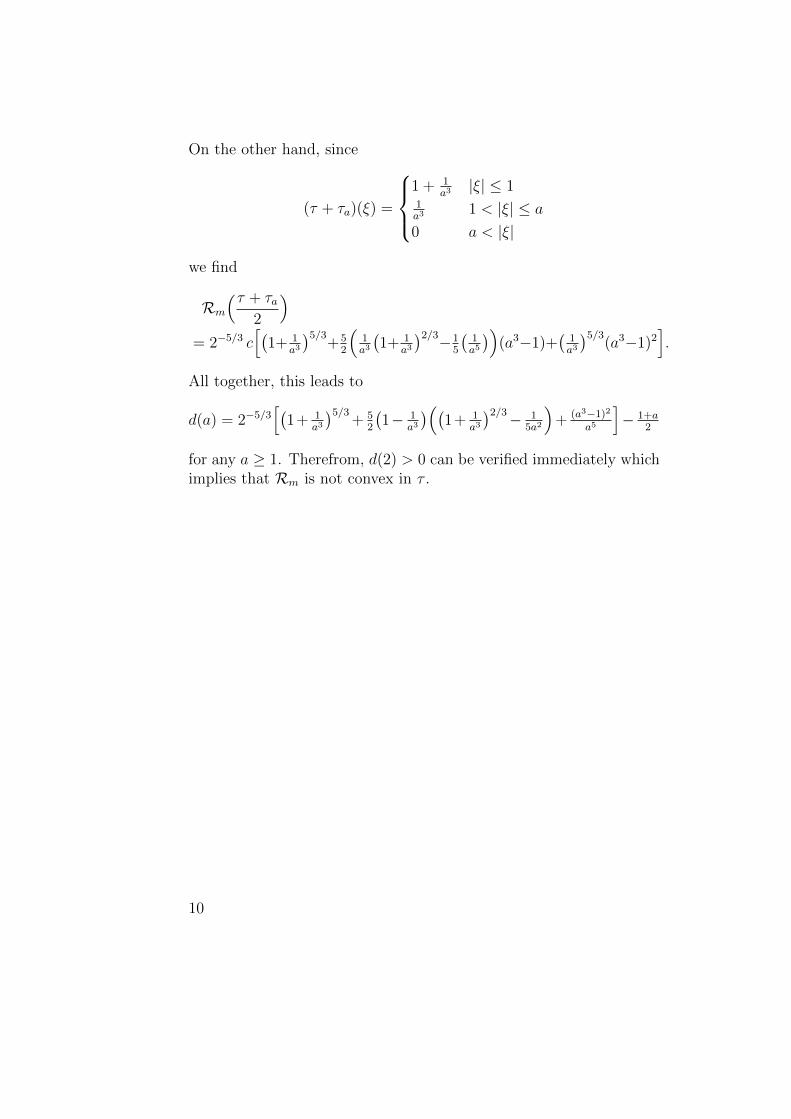
On the other hand, since

(τ + τa)(ξ) =

1 + 1

a3|ξ| ≤ 1

1a3

1 < |ξ| ≤ a

0 a < |ξ|

we find

Rm

(τ + τa2

)= 2−5/3 c

[(1+ 1

a3

)5/3+5

2

(1a3

(1+ 1

a3

)2/3−15

(1a5

))(a3−1)+

(1a3

)5/3(a3−1)2

].

All together, this leads to

d(a) = 2−5/3[(

1+ 1a3

)5/3+ 5

2

(1− 1

a3

)((1+ 1

a3

)2/3− 15a2

)+ (a3−1)2

a5

]− 1+a

2

for any a ≥ 1. Therefrom, d(2) > 0 can be verified immediately whichimplies that Rm is not convex in τ .

10

2. The Functional Es

We introduce a further functional. It is strictly convex and so closelyrelated to EmTF that we may treat this new functional instead of EmTF

when investigating the existence and uniqueness of a minimizing den-sity.

Let the functional Es of the momentum density τ ≥ 0 be given by

Es(τ) :=

∫R3

dξ ξ2τ(ξ)32 − 3

2γ−1/2TF Z

∫R3

dξ τ(ξ)

+ 34γ−1/2TF

∫R3

dξ

∫R3

dη(τ<(ξ, η)

32 τ>(ξ, η)− 1

5τ<(ξ, η)

52

)(2.1)

where τ< and τ> are defined analogously to τ< and τ>, respectively.Indeed, Es is derived from EmTF(τ) by substituting τ → τ 3/2, i. e.,

Es(τ) := EmTF(τ 3/2). (2.2)

In analogy to EmTF we define the sets

J s :={τ ∈ L3/2(R3, (1 + ξ2)dξ) | τ ≥ 0

},

J sN :=

{τ ∈ J s |

∫R3 dξ τ(ξ)

32 ≤ N

},

J s∂N :=

{τ ∈ J s |

∫R3 dξ τ(ξ)

32 = N

}.

Theorem 2.1 (Conta and Siedentop [27]). Es is well-defined on J s.In particular, τ ∈ J s implies τ ∈ L1(R3, dξ).

Proof. By construction (Eq. (2.2)) the finiteness of Es follows fromthe same estimates as in the proof of Theorem 1.1 when substitutingτ → τ 3/2.

Uniqueness of a minimizer, given that it exists, is an importantconsequence of strict convexity. The treatment of the functional Es ishighly motivated by this particular property.

11

Lemma 2.2 (Conta and Siedentop [27, Lemma 1]). The functional Esis strictly convex on all of J s and on any convex subset of J s.

Proof. Let τ ∈ J s# where J s

# denotes J s or any convex subset of J s,e. g., J s

N or J s∂N . Obviously, the first term of Es is strictly convex, the

second is linear. Thus, it suffices to show convexity of the repulsionterm. Let θ denote the Heaviside function, i. e., θ(x) = 1 if x ≥ 0and θ(x) = 0 otherwise, and define the positive part for x ∈ R by[x]+ := max{0, x}. Then, we get∫ ∞

0

dr(∫

R3

dξ [τ(ξ)− r2]+)2

=

∫R3

dξ

∫R3

dη

∫ ∞0

dr [τ(ξ)− r2][τ(η)− r2]θ(τ(ξ)− r2)θ(τ(η)− r2)

=

∫R3

dξ

∫R3

dη

∫ τ<(ξ,η)1/2

0

dr(τ(ξ)τ(η)− τ(ξ)r2 − τ(η)r2 + r4

)=

∫R3

dξ

∫R3

dη(τ(ξ)τ(η)τ<(ξ, η)

12 − 1

3τ(ξ)τ<(ξ, η)

32

− 13τ(η)τ<(ξ, η)

32 + 1

5τ<(ξ, η)

52

)=

∫R3

dξ

∫R3

dη(τ>(ξ, η)τ<(ξ, η)

32 − 1

3τ>(ξ, η)τ<(ξ, η)

32

− 13τ<(ξ, η)

52 + 1

5τ<(ξ, η)

52

)= 2

3

∫R3

dξ

∫R3

dη(τ<(ξ, η)

32 τ>(ξ, η)− 1

5τ<(ξ, η)

52

).

The assertion follows from this identity since the term in the first lineis obviously convex.

Corollary 2.3 (Conta and Siedentop [27]). Let J s# denote J s or any

convex subset of J s, e. g., J sN or J s

∂N . Then there is at most oneτ ∈ J s

# such thatEs(τ) = inf

σ∈J s#Es(σ).

Proof. Let τ1, τ2 ∈ J s#. Suppose τ1 6= τ2 were minimizers of the

functional, i. e., Es(τ1) = Es(τ2) = inf τ∈J s# Es(τ). This contradicts

Es( τ1+τ22) < inf τ∈J s# Es(τ), and therefore the strict convexity of Es.

12

The proof of Lemma 2.2 offers an expedient integral representationfor the electron-electron interaction term of Es:

Definition 2.4. We write the electron-electron interaction term of Esin the following convention:

Rsm(τ) = 9

8γ−1/2TF

∫ ∞0

dr(∫

R3

dξ [τ(ξ)− r2]+)2.

13

3. Thomas-Fermi and the MomentumEnergy Functional

We wish to relate the momentum energy functional given in the firstchapter with the Thomas-Fermi functional. To this end, we first brieflyrecall the definition of the Thomas-Fermi functional and some resultswe will refer to in the sequel. Then, we define explicit transformswhich, eventually, the relation of the two functionals emerges from.

3.1. A Few Results on the Thomas-Fermi Functional

In the chosen units where ~ = 2m = |e| = 1 the well-known Thomas-Fermi functional (Lenz [8]) reads

ETF(ρ) := K(ρ)−A(ρ) +R(ρ) (3.1)

= 35γTF

∫R3

dx ρ(x)53 −

∫R3

dxZ

|x|ρ(x) +D[ρ] (3.2)

where D[ρ] is the quadratic form of

D(ρ, σ) := 12

∫R3

dx

∫R3

dyρ(x)σ(y)

|x− y|(3.3)

for one-particle electron densities ρ and σ in position space. TheThomas-Fermi constant is given as before by γTF = (6π2/q)2/3. Math-ematically this functional has been studied in detail by Lieb andSimon [12, 13] and Lieb [10]. The Thomas-Fermi functional is well-defined for functions in L1(R3) ∩ L5/3(R3) and we write

I :={ρ ∈ L1(R3) ∩ L5/3(R3) | ρ ≥ 0

},

IN :={ρ ∈ I |

∫R3 dx ρ(x) ≤ N

},

I∂N :={ρ ∈ I |

∫R3 dx ρ(x) = N

}

15

for densities in position space.In the following we will use the notion of spherically symmetric

rearrangement, namely,

Definition 3.1. Let A ⊂ R3 and let |A| denote its Lebesgue measure.If |A| < ∞ then A∗ is defined to be the closed ball centered at theorigin which has the same volume as A. We call A∗ the sphericallysymmetric rearrangement of A.

For any function ρ ∈ Lp(R3), 1 ≤ p < ∞ its spherically symmetricrearrangement ρ∗ is given by

ρ∗(x) :=

∫ ∞0

dt χ{x∈R3||ρ(x)|>t}(x)

where χA denotes the characteristic function of the set A.

Now, the property of the Thomas-Fermi functional we want to men-tion first is that it decreases under spherically symmetric rearrange-ment, i. e.,

Lemma 3.2 (Lieb [10, Theorem 2.12]). Let ρ ∈ I and let ρ∗ denoteits spherically symmetric rearrangement. Then

ETF(ρ∗) ≤ ETF(ρ). (3.4)

Other important results we will employ are collected in the followingtheorem:

Theorem 3.3 (Lieb and Simon [13, Theorems II.14, II.17, II.18, II.20]).Let Z ≥ 0.

1. For all 0 ≤ N ≤ Z there exists a unique minimizer ρN of ETF

on I∂N .

2. For N > Z there exists no minimizer of ETF on I∂N .

3. For each N ≥ 0 there exists a unique minimizer ρN of ETF onIN . Moreover, ρN ∈ I∂min{N,Z}.

4. Let ρZ be the unique minimizer of ETF on I∂Z. Then, for allρ ∈ I,

ETF(ρ) ≥ ETF(ρZ).

16

The minimum of the Thomas-Fermi functional is an approximationof the ground state energy. More precisely, suppose the ratio N/Z isfixed, then

inf σ(HN) = infρ∈INETF(ρ) + o(Z7/3).

Moreover, there is a quantum mechanical limit for the density as well.For the case of a neutral atom, i. e., N = Z, we have that

Z−2ρψZ ( ·Z−1/3)→ Z−2ρZ( ·Z−1/3) = ρ1 (3.5)

weakly in the limit Z → ∞. Here, ρψZ denotes the one-particle den-sity of the quantum atom of charge Z and ρZ is the Thomas-Fermiminimizer. These results, among others, assert Thomas-Fermi theoryin the regime of quantum mechanics and give rise to determine thelinear response of atoms to perturbations that are local in positionspace.

We aim to prove some basic mathematical properties of EmTF. Infact, we show equivalent results to Lemma 3.2 and Theorem 3.3 for themomentum functional EmTF. This will establish the functional EmTF

in the regime of quantum mechanics. We will consider momentumdependent perturbations as well.

3.2. Transforms between Position and MomentumFunctional

Now, we define the explicit transforms which transfer each term ofEmTF to the associated term of ETF as long as spherically symmetricdecreasing densities are concerned. We set

S : L1(R3)→ L1(R3)

τ 7→ ρ (3.6)

where ρ is given by

ρ(x) := q(2π)3

∫|x|<γ1/2TF |τ(ξ)|1/3

dξ (3.7)

for all x ∈ R3.

17

For any function ρ ∈ L1(R3) and for any s ≥ 0 we define the Fermiradius r by

r(s) := 0 if γ1/2TF |ρ(x)|1/3 ≤ s for a.e. x ∈ R3,

r(s) := inf{K | γ1/2TF |ρ(x)|1/3 > s for a.e. |x| ≤ K} otherwise.

(3.8)

This infimum can be understood, in some sense, as an essential supre-mum of the set {|x| | γ1/2TF |ρ(x)|1/3 > s}, especially if ρ is sphericallysymmetric. Now, based on the definition of the Fermi radius r we set

T : L1(R3)→ L1(R3)

ρ 7→ τ (3.9)

where τ is given by

τ(ξ) := γ−3/2TF r(|ξ|)3 (3.10)

for all ξ ∈ R3.

The first operator will be used to transfer a momentum densityinto a position density and the second to transfer a position into amomentum density. With this in view we prove the following resultson the operators S and T .

Lemma 3.4 (Conta and Siedentop [27, Lemma 4]).

1. The operator S is isometric on L1(R3).

2. If ρ ∈ L1(R3) and |ρ| spherically symmetric decreasing then

‖T (ρ)‖1 = ‖ρ‖1.

3. All elements in the image of S are spherically symmetric, non-negative, and decreasing.

4. For every spherically symmetric ρ ∈ L1(R3), its image T (ρ) isspherically symmetric, nonnegative, and decreasing.

18

Proof. 1. The claim follows easily by direct computation interchangingthe integration with respect to x and the integration with respect toξ.

2. To treat T we may, without loss of generality, assume ρ ≥ 0.Let ξ ∈ R3. By definition of r and since ρ is spherically symmetricdecreasing

|x| < r(|ξ|)⇒ γ1/2TF ρ(x)1/3 > |ξ| (3.11)

for almost every x ∈ R3, in the sense that almost every x ∈ R3 with|x| < r(|ξ|) satisfies γ

1/2TF ρ(x)1/3 > |ξ|. Likewise, the definition of r

provides that|x| ≤ r(|ξ|)⇐ γ

1/2TF ρ(x)1/3 > |ξ| (3.12)

for almost every x ∈ R3.We have

‖T (ρ)‖1 = 3

4πγ3/2TF

∫dξ

∫|x|<r(|ξ|)

dx. (3.13)

By (3.11) we get the estimate

‖T (ρ)‖1 ≤ 3

4πγ3/2TF

∫dξ

∫γ1/2TF ρ(x)

1/3>|ξ|dx

= 3

4πγ3/2TF

∫dx

∫γ1/2TF ρ(x)

1/3>|ξ|dξ =

∫dx ρ(x). (3.14)

On the other hand, if we allow for ≤ instead of strict inequality onthe integration constraints in (3.13) we can also reverse the inequalityin (3.14) using (3.12).

3. and 4. The claims follow directly from the definitions.

Now, we will see how the functionals ETF and EmTF are related viathe operators S and T , namely,

Lemma 3.5 (Conta and Siedentop [27, Lemma 4]).

1. For every spherically symmetric decreasing τ ∈ J

EmTF(τ) = ETF ◦ S(τ).

2. For every spherically symmetric decreasing ρ ∈ I

EmTF ◦ T (ρ) = ETF(ρ).

19

Proof. 1. We treat each term of the energy functional individually. Westart with the potential terms, actually with the external potentialwhich is an easy variant of the interaction potential. Both follow byexplicit calculation.

We have

A(S(τ)) =

∫dx

Z

|x|S(τ)(x) = Z

∫dx q

(2π)3

∫|x|<γ1/2TF τ(ξ)

1/3

dξ1

|x|

= Z

∫dξ q

(2π)34π2γTF τ(ξ)

23 = 3

2γ−1/2TF Z

∫dξ τ(ξ)

23 . (3.15)

Now we exhibit the calculation for the interaction potential. Givena radius a > 0 we set Ka := χ{x∈R3||x|<a} to be the characteristicfunction of the open ball of radius a centered at the origin. We get

R(S(τ)) = 12

∫dx

∫dy

1

|x− y|(q

(2π)3

)2 ∫|x|<γ1/2TF τ(ξ)

1/3

dξ

∫|y|<γ1/2TF τ(η)

1/3

dη (3.16)

=(

q(2π)3

)2 ∫∫dξdη D(K

γ1/2TF τ(ξ)

1/3 , Kγ1/2TF τ(η)

1/3) (3.17)

=(

34π

)2γ−1/2TF

∫∫dξdη D(K 3

√τ<(ξ,η)

, K 3√τ>(ξ,η)

) (3.18)

= 9(4π)2

γ−1/2TF

(∫∫dξdη D[K 3

√τ<(ξ,η)

]

+

∫∫dξdη D(K 3

√τ<(ξ,η)

, K 3√τ>(ξ,η)

−K 3√τ<(ξ,η)

))

(3.19)

= 9(4π)2

γ−1/2TF

(∫∫dξdη D[K 3

√τ<(ξ,η)

]

+

∫∫dξdη 1

2

∫|x|< 3√τ<(ξ,η)

dx

∫3√τ<(ξ,η)≤|y|< 3

√τ>(ξ,η)

dy1

|y|

)(3.20)

= 9(4π)2

γ−1/2TF

(∫∫dξdη D[K1]τ<(ξ, η)

53

+

∫∫dξdη 4π

2·3 τ<(ξ, η)2π(τ>(ξ, η)

23 − τ<(ξ, η)

23

))(3.21)

= 34γ−1/2TF

∫∫dξdη τ<(ξ, η)τ>(ξ, η)

23 − 1

5τ<(ξ, η)

53 (3.22)

20

where we used the scaling properties of D in (3.18) and Newton’s

Theorem B.5 to get (3.20). In particular, D[K1] = (4π)2

15follows by a

simple computation.Now we turn to the remaining term, the kinetic energy. It trans-

forms as

K(S(τ)) = 35γTF

∫dxS(τ)(x)

53 = 3γTF

∫dx

∫0≤t≤S(τ)(x)1/3

dt t4

= 34πγTF

∫dξξ2

∫|ξ|3≤S(τ)(x)

dx. (3.23)

Given that S(τ)(x) ≥ |ξ|3 implies γ1/2TF τ(γ

1/2TF ξ)

1/3 ≥ |x|, which is equiv-alent to the statement that 3

4π

∫|x|<τ(η)1/3 dη ≥ |ξ|3 implies τ(ξ)1/3 ≥

|x|, we have

35γTF

∫dxS(τ)(x)

53 ≤ 3

4πγTF

∫dξ ξ2

∫|x|≤γ1/2TF τ(γ

1/2TF ξ)

1/3

dx (3.24)

=

∫dξ ξ2τ(ξ). (3.25)

Suppose 34π

∫|x|<τ(η)1/3 dη ≥ |ξ|3 would not imply τ(ξ)1/3 ≥ |x|. Then

|ξ|3 ≤ 34π

∫|x|<τ(η)1/3

dη < 34π

∫τ(ξ)<τ(η)

dη ≤ 34π

∫|ξ|>|η|

dη = |ξ|3 (3.26)

where we used in the last inequality that τ is spherically symmetricand decreasing.

On the other hand, 34π

∫|x|<τ(η)1/3 dη ≥ |ξ|3 follows from τ(ξ)1/3 > |x|

as

|ξ|3 = 34π

∫|η|≤|ξ|

dη ≤ 34π

∫τ(ξ)≤τ(η)

dη ≤ 34π

∫|x|<τ(η)1/3

dη (3.27)

using in the first inequality again that τ is spherically symmetric anddecreasing. Thus we can reverse the inequality in (3.24), i. e.,

35γTF

∫dxS(τ)(x)

53 ≥ 3

4πγTF

∫dξ ξ2

∫|x|<γ1/2TF τ(γ

1/2TF ξ)

1/3

dx (3.28)

=

∫dξ ξ2τ(ξ). (3.29)

21

2. To prove that EmTF ◦T (ρ) = ETF(ρ) we proceed as in 1. We beginwith the kinetic energy:

Km(T (ρ)) =

∫dξ ξ2γ

−3/2TF r(|ξ|)3 = 3

4πγ−3/2TF

∫dξ ξ2

∫|x|<r(|ξ|)

dx

= 34πγ−3/2TF

∫dξ ξ2

∫|ξ|<γ1/2TF ρ(x)

1/3

dx = K(ρ) (3.30)

where we used (3.11) and (3.12) in the penultimate identity.For the external potential we get

Am(T (ρ)) = 32γ−3/2TF Z

∫dξ r(|ξ|)2 = 3γ

−3/2TF Z

∫dξ

∫0≤t<r(|ξ|)

dt t

= Z 34πγ−3/2TF

∫dξ

∫|x|<r(|ξ|)

dx 1|x| = Z 3

4πγ−3/2TF

∫dx 1|x|

∫|ξ|<γ1/2TF ρ(x)

1/3

dξ

= Z

∫dx

1

|x|ρ(x) (3.31)

using again (3.11) and (3.12) in the penultimate identity.Finally we go to Rm. Adapting the steps (3.22) to (3.16) yields

Rm(T (ρ)) = 12

∫∫dxdy

1

|x− y|(

q(2π)3

)2 ∫|x|<r(|ξ|)

dξ

∫|y|<r(|η|)

dη

= 12

(q

(2π)3

)2 ∫∫dxdy

1

|x− y|

∫|ξ|<γ1/2TF ρ(x)

1/3

dξ

∫|η|<γ1/2TF ρ(y)

1/3

dη

= R(ρ) (3.32)

using (3.11) and (3.12) once more.

22

4. Results on the Minimal Energyand the Minimizer

4.1. Existence and Uniqueness Results

The following theorem establishes EmTF as the momental analogue ofthe Thomas-Fermi functional (cf. Theorem 3.3).

Theorem 4.1 (Conta and Siedentop [27, Theorem 2]). Let Z ≥ 0.

1. For all N ≥ 0, we have infτ∈J∂N EmTF(τ) = infρ∈I∂N ETF(ρ).

2. Let 0 ≤ N ≤ Z. If ρN is the unique minimizer of ETF on I∂Nthen T (ρN) is the unique minimizer of EmTF on J∂N .

3. For N > Z there exists no minimizer of EmTF on J∂N .

4. For each N ≥ 0 there exists a unique minimizer τN of EmTF onJN . Moreover, τN ∈ J∂min{N,Z}.

5. Let τZ be the unique minimizer of EmTF on J∂Z. Then, for allτ ∈ J ,

EmTF(τ) ≥ EmTF(τZ).

The proof of Theorem 4.1 is based on the relation of the functionalsETF and EmTF that was indicated in Lemma 3.5. Thus, in order toapply this lemma we want to restrict the two functionals to spher-ically symmetric decreasing densities. We overcome this problem ifwe can ensure that EmTF decreases under spherically symmetric rear-rangement since the same result holds for ETF (Lemma 3.2).

Lemma 4.2 (Conta and Siedentop [27, Lemma 5]). Let τ ∈ J andlet τ ∗ denote its spherically symmetric rearrangement (Definition 3.1).Then

EmTF(τ ∗) ≤ EmTF(τ). (4.1)

23

Proof. The attraction Am is obviously invariant under rearrangement.The repulsion Rm is – by definition – a superposition of rearrangedterms only, i. e., is also trivially invariant.

Let |A| denote the Lebesgue measure of any subset A of R3. SinceKm(τ) =

∫∞0

dt∫

dξ ξ2χ{ξ∈R3|τ(ξ)>t}(ξ), it suffices to show that for anyA ⊂ R3 with finite measure∫

dξ ξ2χA(ξ) ≥∫

dξ ξ2χA∗(ξ) =

∫|ξ|≤R

dξ ξ2

where R is defined by |A| = 4π3R3, i. e., the radius of the ball A∗ :=

BR(0) centered at the origin which has the same volume as A. Nowdefine the sets B := BR(0) \A, C := A \BR(0), and D := A∩BR(0).Then |B| = |C|, and thus∫

A∗dξ ξ2 =

∫B

dξ ξ2 +

∫D

dξ ξ2 ≤ R2

∫B

dξ +

∫D

dξ ξ2

≤∫C

dξ ξ2 +

∫D

dξ ξ2 =

∫A

dξ ξ2.

Corollary 4.3 (Conta and Siedentop [27]). Every minimizer τ ∈ Jof EmTF is spherically symmetric decreasing.

Now, we can prove Theorem 4.1:

Proof. 1. The two functionals ETF and EmTF decrease under sphericallysymmetric rearrangement (Lemma 3.2 and Lemma 4.2). So, as far asminimization is concerned, we may restrict both functionals to spheri-cally symmetric decreasing densities ρ and τ . Under this restriction Sand T preserve the norm and hence Statement 1 of Lemma 3.5 impliesthat

infτ∈J∂N

EmTF(τ) ≥ infρ∈I∂N

ETF(ρ)

whereas Statement 2 implies the reverse inequality. This proves thefirst assertion of Theorem 4.1.

2. Since ETF has a unique minimizer ρN on I∂N if N ≤ Z (Theo-rem 3.3), it follows from the preceding step and Lemma 3.5, State-ment 2 that T (ρN) minimizes EmTF on J∂N .

24

It remains to show that there is no other minimizer of the momen-tum functional. This follows from the strict convexity of Es (Lem-ma 2.2). Indeed, suppose that τN 6= τ ′N were two different minimiz-ers of EmTF on J∂N . Then, since infτ∈J∂N EmTF(τ) = infτ∈J s∂N Es(τ)(Eq. (2.2)), we obtain two different minimizers τN 6= τ ′N of Es on J s

∂N

from the substitutions τ3/2N = τN and (τ ′N)3/2 = τ ′N . But this contra-

dicts Corollary 2.3.3. Suppose τN is a minimizer of EmTF on J∂N for some N > Z. Then

S(τN) has to be a minimizer of ETF by Statement 1 and Lemma 3.5,Statement 1 but this does not exist (Theorem 3.3).

4. Again, if τN minimizes EmTF on JN then S(τN) minimizes ETF onIN . Thus,

∫τN =

∫S(τN) = min{Z,N}. Uniqueness of τN follows

from the strict convexity of Es as in the proof of Statement 2.5. The claim follows from Statement 2 and Statement 4.

4.2. Properties of the Minimizing Density and Euler’sEquation

We start with a bound on the minimizer. By the definition of T , therelation between r and τ as given by (3.10), and Theorem 4.1 anybound on the position space density implies a corresponding boundon the momentum space density.

Lemma 4.4 (Conta and Siedentop [27]). Let τ be the minimizer ofEmTF on J , then

τ(ξ) ≤ γ−3/2TF

Z3

|ξ|6(4.2)

for almost every ξ ∈ R3. Furthermore, there exists ξ0 ∈ R3 \ {0} suchthat

τ(ξ) ≤(3π

) 32γ−3/2TF

1

|ξ|3/2(4.3)

for almost every ξ ∈ R3 satisfying |ξ| < |ξ0|.

Proof. Let ρ be the Thomas-Fermi minimizer on I. Then ρ obeys

ρ(x) ≤ γ−3/2TF

Z3/2

|x|3/2

25

for almost every x ∈ R3 as a consequence of the corresponding Eulerequation in position space (see, e. g., Lieb and Simon [13]). This im-plies the first bound in the proposition since τ can be represented interms of ρ by means of T as defined in Eq. (3.10). In this case,

τ(ξ) = T (ρ)(ξ)

= γ−3/2TF

(inf{K | γ1/2TF |ρ(x)|1/3 > |ξ| for a.e. |x| ≤ K}

)3= γ

−3/2TF

(inf{K | Z

1/2

|x|1/2≥ γ

1/2TF |ρ(x)|1/3 > |ξ| for a.e. |x| ≤ K

})3≤ γ

−3/2TF

(sup{|x| | Z

1/2

|x|1/2> |ξ|

})3= γ

−3/2TF

(sup{|x| | Z

|ξ|2> |x|

})3≤ γ

−3/2TF

( Z

|ξ|2)3

= γ−3/2TF

Z3

|ξ|6(4.4)

for almost every ξ ∈ R3. Indeed, the infimum exists as ρ is unbounded(see, e. g., Lieb and Simon [13]).

Likewise, the second bound in the proposition is a consequence ofthe Sommerfeld bound [13, 25] concerning the asymptotics of ρ at in-finity. In position space there exists some x0 ∈ R3 \ {0} such that

ρ(x) ≤ 27π−3γ−3/2TF

1

|x|6

for almost every x ∈ R3 with |x| ≥ |x0|. Moreover, since ρ is spheri-cally symmetric decreasing (Lemma 3.2) we can find some ξ0 ∈ R3\{0}such that γ

1/2TF ρ(x)1/3 ≥ |ξ0| for almost every |x| < |x0|. Thus, for al-

most every ξ ∈ R3 with |ξ| < |ξ0| we get

τ(ξ) = γ−3/2TF

(inf{K | γ1/2TF |ρ(x)|1/3 > |ξ| for a.e. |x| ≤ K}

)3= γ

−3/2TF

(inf{K | γ1/2TF |ρ(x)|1/3 > |ξ| for a.e. |x0| ≤ |x| ≤ K}

)3≤ γ

−3/2TF

(sup{|x| | 3π−1 1

|x|2> |ξ|

})3

26

= γ−3/2TF

(sup{|x| |

(3π

)1/2 1

|ξ|1/2> |x|

})3≤(3π

)3/2γ−3/2TF

1

|ξ|3/2. (4.5)

Note that the second identity holds since ρ is spherically symmetricdecreasing.

The following property of the minimizer will be applied for thederivation of the Euler equation hereafter.

Lemma 4.5 (adapted from Conta and Siedentop [27, Lemma 2]). Theminimizer of EmTF on J is strictly positive almost everywhere. More-over, the minimizer of EmTF on JN for each N > 0 is strictly positivealmost everywhere.

Proof. Let τ be a minimizer of EmTF. Suppose that the set Nτ :={ξ ∈ R3|τ(ξ) = 0}, on which τ vanishes, would not be of measure zero.Then pick any function σ ∈ J with τ(ξ)σ(ξ) = 0 for almost all ξ ∈ R3

which is not identical zero onNτ and satisfies∫R3 dξ σ(ξ) ≤

∫R3 dξ τ(ξ).

For any 0 < ε ≤ 1 we define the function

τε := τ + ε(σ −

∫σ∫ττ).

Note that τε ∈ J and∫τε =

∫τ . Then by the integral representation

of the interaction term (Definition 2.4) together with the substitutionτ 3/2 = τ we get

EmTF(τε)− EmTF(τ)

= 32γ−1/2TF Z

∫R3

dξ(

1−(1− ε

∫σ∫τ

) 23

)τ(ξ)

23 − 3

2γ−1/2TF Z

∫R3

dξ ε2/3σ(ξ)23

+ 32· 34γ−1/2TF

∫ ∞0

dr(∫

R3

dξ[(

1− ε∫σ∫τ

) 23 τ(ξ)

23 − r2]+

+

∫R3

dξ [ε2/3σ(ξ)23 − r2]+

)2− 3

2· 34γ−1/2TF

∫ ∞0

dr(∫

R3

dξ [τ(ξ)23 − r2]+

)2+O(ε) (4.6)

27

≤ −ε2/3 32γ−1/2TF Z

∫R3

dξ σ(ξ)2/3 +O(ε)

+ 32· 34γ−1/2TF

∫ ∞0

dr(∫

R3

dξ [τ(ξ)23 − r2]+

+

∫R3

dξ [ε2/3σ(ξ)23 − r2]+

)2− 3

2· 34γ−1/2TF

∫ ∞0

dr(∫

R3

dξ [τ(ξ)23 − r2]+

)2(4.7)

= −ε2/3 32γ−1/2TF Z

∫R3

dξ σ(ξ)23 +O(ε)

+ 2 · 34· 32γ−1/2TF

∫ ∞0

dr(∫

R3

dξ [τ(ξ)23 − r2]+

)×(∫

R3

dη[ε2/3σ(η)23 − r2]+

)(4.8)

≤ −ε2/3 32γ−1/2TF Z

∫R3

dξ σ(ξ)23 +O(ε)

+ 94γ−1/2TF

[∫ ∞0

dr(∫

R3

dξ [τ(ξ)23 − r2]+

)2] 12

×[∫ ∞

0

dr(∫

R3

dη [ε2/3σ(η)23 − r2]+

)2] 12

= −ε2/3 32γ−1/2TF Z

∫R3

dξ σ(ξ)23 +O(ε5/6) (4.9)

where in the first inequality we used that 1−ε∫σ∫τ≤(1−ε

∫σ∫τ

)2/3 ≤ 1.

In the second inequality we applied the Cauchy-Schwarz inequality.And finally, scaling the powers of ε out yields the given estimate.

In fact, this implies that

EmTF(τε)− EmTF(τ) < 0,

for sufficiently small ε. Hence, τ cannot be a minimizer.

Now, we turn to the proof of Euler’s equation.

Lemma 4.6 (Conta and Siedentop [27, Lemma 3]). The Euler equa-tion which the minimizer of EmTF on J satisfies is

γ1/2TF |ξ|

2τ(ξ)13 − Z +

∫R3

dη(32τ(η)

23 τ<(ξ, η)

13 − 1

2τ<(ξ, η)

)= 0. (4.10)

28

Proof. Instead of deriving the Euler equation for EmTF we use Es (seeEq. (2.2)).

Let τ be the minimizer which is strictly positive almost everywherebecause of Lemma 4.5. Thus we can pick any σ ∈ L3/2(R3, (1 + ξ2)dξ)with |σ| ≤ τ . Then, for ε ∈ [−1, 1], τ + εσ is an allowed trial functionand the function F (ε) = Es(τ + εσ) has a minimum at zero. We showthat F is differentiable at zero.

The first two terms of F are obviously differentiable. For the deriva-tive of the kinetic term we obtain 3

2

∫R3 dξ ξ2σ(ξ)τ(ξ)1/2 at ε = 0 and

for the derivative of the external potential evaluated at the origin weget 3

2γ−1/2TF Z

∫R3 dξ σ(ξ). Thus, we concentrate on

T (ε) := ε−1∫ ∞0

dr[(∫

R3

dξ [τ(ξ) + εσ(ξ)− r2]+)2

−(∫

R3

dξ [τ(ξ)− r2]+)2]

=

∫ ∞0

dr

∫R3

dξ

∫R3

dη[τ(ξ) + εσ(ξ)− r2]+ − [τ(ξ)− r2]+

ε

×([τ(η) + εσ(η)− r2]+ + [τ(η)− r2]+

)=:

∫ ∞0

dr

∫R3

dξ

∫R3

dη I(ε, r, ξ, η).

(4.11)

Since |a+−b+| ≤ |a−b| for real a and b (Lemma B.1) and since |ε| ≤ 1we get

|σ(ξ)|([τ(η) + |σ(η)| − r2]+ + [τ(η)− r2]+

)to be an integrable majorant of the integrand I independent of ε.Indeed, we have∫ ∞

0

dr

∫R3

dξ

∫R3

dη |σ(ξ)|[τ(η) + |σ(η)| − r2]+

≤∫R3

dξ |σ(ξ)|∫ ∞0

dr

∫R3

dη [2τ(η)− r2]+

=

∫R3

dξ |σ(ξ)| 23

∫R3

dη 23/2 τ(η)32 <∞ (4.12)

29

as |σ| ≤ τ . Now, to apply dominated convergence, we split the integralin two parts, namely the part where the pointwise limit of I exists andthe rest. Consider [a+εb]+−[a]+

εfor a, b ∈ R in the limit where ε tends

to zero. In the case where a = 0, this limit does not exist. Whereas,if a < 0 then [a+εb]+−[a]+

ε→ 0, and if a > 0 then [a+εb]+−[a]+

ε→ b. In

summary, [a+ εb]+ → [a]+ as ε→ 0 for a 6= 0. This finally results in

limε→0

T (ε) = limε→0

∫ ∞0

dr

∫τ(ξ)=r2

dξ

∫R3

dη I(ε, r, ξ, η)

+ limε→0

∫ ∞0

dr

∫τ(ξ)6=r2

dξ

∫R3

dη I(ε, r, ξ, η)

= 2

∫ ∞0

dr

∫R3

dξ

∫R3

dη σ(ξ)θ(τ(ξ)− r2)[τ(η)− r2]+.

(4.13)

Indeed, the integration with respect to r restricted to τ(ξ) = r2 yieldszero.

In fact, this proves that F is differentiable. Hence, integration withrespect to r yields

∫R3

dξ σ(ξ)[32ξ2τ(ξ)

12 − 3

2γ−1/2TF Z

+ 32· 34γ−1/2TF

∫R3

dη(2 τ(η)τ<(ξ, η)

12 − 2

3τ<(ξ, η)

32

)]= 0. (4.14)

Since σ is arbitrary we arrive at the desired Euler equation (4.10) aftersubstituting τ 3/2 = τ .

Since the integrand in (4.10) is nonnegative, the Euler equationimplies the following pointwise bound on the minimizer:

τ(ξ) ≤ γ−3/2TF

Z3

|ξ|6. (4.15)

In particular, this bound we got already from Lemma 4.4.

30

4.3. The Virial Theorem

Theorem 4.7 (Virial Theorem). If τ minimizes EmTF on any JN ,then

2Km(τ) = Am(τ)−Rm(τ). (4.16)

Proof. Suppose τ is the minimizer of EmTF on JN and define τλ(ξ) :=λ−3τ(λ−1ξ) for some λ > 0. Note that τλ ∈ JN with ‖τλ‖1 = ‖τ‖1.Scaling yields

EmTF(τλ) = λ2Km(τ)− λAm(τ) + λRm(τ). (4.17)

Consider EmTF(τλ) as a function of λ. Then EmTF(τλ) is differentiablefor positive λ and has its unique minimum at λ = 1. Thus,

0 =dEmTF(τλ)

dλ

∣∣∣∣λ=1

= 2Km(τ)−Am(τ) +Rm(τ). (4.18)

If τ is the minimizer of EmTF on J then another relation betweenKm(τ), Am(τ), and Rm(τ) can be easily achieved via minimization,namely,

Theorem 4.8. If τ minimizes EmTF on J , then

3Km(τ) = 2Am(τ)− 5Rm(τ). (4.19)

Proof. Suppose τ is the minimizer of EmTF on J and define τλ(ξ) :=λτ(ξ) for some λ > 0. Then the same reasoning as in the precedingproof gives

0 =dEmTF(τλ)

dλ

∣∣∣∣λ=1

= Km(τ)− 23Am(τ) + 5

3Rm(τ). (4.20)

Corollary 4.9. If τ minimizes EmTF on J , then the following ratioholds:

Km(τ) : Am(τ) : Rm(τ) = 3 : 7 : 1.

31

Proof. The assertion follows from (4.16) and (4.19).

Remark. The Virial Theorem can be also obtained using the opera-tor T and the Virial Theorem for ETF (Lieb and Simon [13, TheoremII.22]). The same applies to the corollary when using the correspond-ing relation between K(ρ), A(ρ), and R(ρ) for the atomic Thomas-Fermi density ρ (Lieb and Simon [13, Corollary II.24]).

32

5. Asymptotic Exactness of Englert’sStatistical Model of the Atom

In this chapter we show that the atomic momentum density convergeson the scale Z2/3 to the minimizer of the momentum energy functionalEmTF. Note that in the semiclassical regime this corresponds to thescale where ~ = Z−1/3 (cf. Eq. (3.5)).

As indicated already in the introduction this limit theorem for thedensity is essential to determine the linear response of atoms to pertur-bations that are local in momentum space. As a result of Theorem 4.1from the previous chapter we already know that the ground state en-ergy is asymptotic to the infimum of the momentum energy functionalEmTF of the same order as the Thomas-Fermi energy is. Therefore,

inf σ(HN) = infτ∈JN

EmTF(τ) + o(Z7/3)

if the ratio N/Z is fixed. Now, we shall consider the HamiltonianHN perturbed by some momentum dependent potential ϕZ(ξ) :=Z4/3ϕ(Z−2/3ξ), namely,

HN,α := HN − αN∑n=1

ϕZ(−i∇n) (5.1)

with some α ∈ R. In fact, in the proposition of the limit theorem wewill have some requirements on α and ϕ.

We shall consider the simultaneous limit Z → ∞, N → ∞ suchthat the ratio N/Z is fixed. In order to simplify notation we avoid theintroduction of a scaling parameter which incorporates the dependenceof N and Z. Moreover, the case where N 6= Z requires the notion ofan approximate ground state. So, we start with the introduction ofsome useful notations:

33

1. Let ψN ∈∧Nn=1 L

2(R3 : Cq) =: H be a sequence of normalizedvectors such that

inf σ(HN)− 〈ψN , HNψN〉Z7/3

→ 0

as Z →∞, N →∞ under the subsidiary condition that N/Z isfixed. We call ψN an approximate ground state of HN .

2. The one-particle ground state density of any normalized vectorψ ∈ H is defined by

ρψ(x) := N

q∑σ1=1

· · ·q∑

σN=1

∫R3(N−1)

dx2 · · · dxN

× |ψ(x, σ1;x2, σ2; . . . ;xN , σN)|2

in position space and

τψ(ξ) := N

q∑σ1=1

· · ·q∑

σN=1

∫R3(N−1)

dξ2 · · · dξN

× |ψ(ξ, σ1; ξ2, σ2; . . . ; ξN , σN)|2

in momentum space where ψ denotes the Fourier transform of ψon∧Nn=1 L

2(R3). The rescaled one-particle momentum densityof ψ is given by

τψ(ξ) := Zτψ(Z2/3ξ).

3. We denote the set of all trace class operators on L2(R3 : Cq) byS1(L2(R3 : Cq)). Then

S := {γ ∈ S1(L2(R3 : Cq)) | 0 ≤ γ ≤ 1}

is called the set of fermionic one-particle density matrices.

4. The one-particle density matrix of a normalized N -particle stateψ ∈ H is denoted by γψ and it satisfies tr γψ = N .

34

5. Every γ ∈ S has a spectral decomposition into orthonormaleigenvectors ej ∈ L2(R3 : Cq) and the corresponding eigenvalues0 ≤ λj ≤ 1. We write

τγ(ξ) :=

q∑σ=1

∑j

λj|ej(ξ, σ)|2

for the momentum density of γ. Here ej denotes the Fouriertransform of ej on L2(R3). The rescaled momentum density ofγ is given by

τγ(ξ) := Zτγ(Z2/3ξ).

6. Let ρN be the minimizer of the Thomas-Fermi functional ETF

on IN (see Theorem 3.3). Then ρN obeys the Thomas-Fermiequation

γTFρ2/3N = [φN − µ]+

where µ is some positive constant and φN denotes the Thomas-Fermi potential which is given by

φN := Z/| · | − ρN ∗ | · |−1.

In particular, µ is uniquely determined by φN . These quantitiesscale as

φN(x) =: φ(Z,N, x) = Z4/3φ(1, N/Z, Z1/3x),

µ =: µ(Z,N) = Z4/3µ(1, N/Z).

For references see, e. g., Lieb and Simon [12] or Lieb [10].

7. For α ∈ R, the effective one-particle Hamiltonian correspondingto the Thomas-Fermi potential is given by

hN,α := −∆− φN − αϕZ(−i∇)

and we write hN,α(ξ, x) for its Hamilton function.

The following lemma provides a lower bound to the sum of thenegative eigenvalues of the one-particle Hamiltonian hN,α.

35

Lemma 5.1 (Neutral Case N = Z: Conta and Siedentop [27, Lemma6]). Let α ∈ R. Let µ ≥ 0 and hN,α be given as in Notation 6 and 7above. Assume 0 ≤ (1 + | · |−2)ϕ ∈ L∞(R3), ϕ uniformly continuous,and |α| < v/2 with v := 1/(‖| · |−2ϕ‖∞). Then, for every γ ∈ S,

tr (hN,αγ) ≥ q(2π)3

∫hN,α(ξ,x)<−µ

dξdxhN,α(ξ, x)− o(Z7/3) (5.2)

uniformly in α for large Z when the ratio N/Z is fixed.

Remark. The corresponding result for the unperturbed one-particleHamiltonian hN,0 can be found in the article of Lieb [10, Section V.A.2].There he shows that, for all γ ∈ S,

tr (hN,0γ) ≥ q(2π)3

∫hN,0(ξ,x)<−µ

dξdxhN,0(ξ, x)− constZ7/3−1/30

if N = O(Z). We will follow his proof modified by the momentumoperator ϕZ .

Proof of Lemma 5.1. Note that due to the Thomas-Fermi equationand the requirements on α and ϕ in the hypothesis of the lemma wehave

q(2π)3


dξdx ≤ q(2π)3

∫12ξ2−φN (x)<−µ

dξdx ≤ constN (5.3)

and likewise

q(2π)3

∫hN,α(ξ,x)<0

dξdxhN,α(ξ, x) ≥ −constZ73

if N = O(Z).Next, we follow the lower bound of Lieb’s asymptotic result (Lieb [10,

Theorem 5.1]). To this end let g ∈ C∞0 (R3) be a spherically symmetricpositive function with supp(g) contained in the unit ball,

∫g2 = 1,

and gR(x) := R3/2g(Rx) its dilatation by R. Note that gR = gR−1

holds for the Fourier transform of gR. Furthermore, let fξ,x(r) :=eiξ·rgR(r − x) be the coherent states in L2(R3) and define the projec-tion πξ,x := |fξ,x〉〈fξ,x| ⊗ Iσ where Iσ denotes the identity operator inspin space.

36

Thus, the identity

q∑σ=1

∫R3

dx |∇xej(x, σ)|2 = 1(2π)3

∫dξdx ξ2〈ej, πξ,xej〉 − ‖ej‖22 ‖∇gR‖22

(5.13)

can be easily verified by

1(2π)3

∫dξdx ξ2〈ej, πξ,xej〉 =

q∑σ=1

∫dξdp (ξ − p)2 |gR(p)|2|ej(ξ, σ)|2

=

q∑σ=1

∫dξdp ξ2 |gR(p)|2|ej(ξ, σ)|2 +

q∑σ=1

∫dξdp p2 |gR(p)|2|ej(ξ, σ)|2

=

q∑σ=1

∫R3

dx |∇xej(x, σ)|2 + ‖ej‖22 ‖∇gR‖22. (5.14)

Indeed, replacing ϕZ by the square function in line (5.7) – line (5.12)yields the first equality. The second holds since g is spherically sym-metric. Eq. (5.4), (5.5), and (5.13) are also stated in the proof ofLieb [10, Theorem 5.1]. It follows that for any γ ∈ S written in theform γ =

∑j λj|ej〉〈ej| (cf. Notation 5) we have

tr (hN,αγ) = 1(2π)3

∫dξdx

(hN,α(ξ, x) + µ1h(ξ, x)

)∑j

λj〈ej, πξ,xej〉

− µ tr1hγ

− tr γR2‖∇g‖22 − tr [(φN − φN ∗ |gR|2)γ]

− α tr[[(ϕZ − ϕZ ∗ |gR|2)(−i∇)]γ

](5.15)

where 1h is the projection to the negative spectral subspace of hN,α+µand 1h(ξ, x) its symbol. Since we are interested in a lower bound wemay assume tr γ ≤ constZ. Furthermore, 0 ≤

∑j λj〈ej, πξ,xej〉 ≤ q

hence

tr (hN,αγ) ≥ q(2π)3


dξdx (hN,α(ξ, x) + µ)

− constZR2‖∇g‖22 − tr [(φN − φN ∗ |gR|2)γ]

− α tr[[(ϕZ − ϕZ ∗ |gR|2)(−i∇)]γ

]. (5.16)

38

The right hand side of the first line is the wanted main term addedby an error term of order O(Z). Indeed, sneaking in the constantµ generates an error term just of the same order as the phase spacevolume (Eq. (5.3)) which is uniformly in α. This is negligible comparedto the error of order o(Z7/3) which the remaining terms bring up.Actually, if we choose R = Z1/2 then the third line consists of errorterms of order O(Z7/3−1/30) (Lieb [10, Theorem 5.1]). The term in thelast line is new and to see that it is a further error term we need anadditional argument.

We have

|tr [(ϕZ(−i∇)− (ϕZ ∗ |gR|2)(−i∇))γ]|

≤ Z7/3

∫R3

dξ

∫R3

dp τγ(ξ)|ϕ(ξ)− ϕ(ξ − p)||gZ1/6(p)|2. (5.17)

However, the integral of the right hand side converges to zero by uni-form continuity of ϕ and the fact that g ∈ S(R3). To see this we showthat ‖ϕ − ϕ ∗ |gZ1/6|2‖∞ is arbitrarily small for large Z: Let ε > 0.Since ϕ is uniformly continuous, there exists δ > 0 such that |p| < δimplies |ϕ(ξ)− ϕ(ξ − p)| < ε

2for all ξ, p ∈ R3.

Note that g is a Schwartz function and hence there exists a constantc > 0 such that

|g(p)|2 < c

|p|4(5.18)

for all p ∈ R3. Moreover, for every ε, there is a Z0 > 0 such that

2Z−1/6c ‖ϕ‖∞∫|p|>δ

dp |p|−4 < ε2

for all Z > Z0. With this choice, we estimate∫R3

dp |ϕ(ξ)− ϕ(ξ − p)||gZ1/6(p)|2

=

∫|p|<δ

dp |ϕ(ξ)− ϕ(ξ − p)||gZ1/6(p)|2

+

∫|p|>δ

dp |ϕ(ξ)− ϕ(ξ − p)||gZ1/6(p)|2

≤ ε2

+ 2‖ϕ‖∞c∫|p|>δ

dpZ1/2

(Z1/6|p|)4≤ ε

2+ ε

2. (5.19)

39

Thus, Z > Z0 implies∫R3

dξ

∫R3

dp τγ(ξ)|ϕ(ξ)−ϕ(ξ−p)||gZ1/6(p)|2 ≤ ε

∫R3

dξ τγ(ξ) = const ε.

This proves that the last line of (5.16) is an error term of order o(Z7/3)and that it is uniformly in α. In fact, this finishes the proof.

Now, the previous lemma allows us to prove the following asymp-totic result for the density of the momentum functional EmTF:

Theorem 5.2 (Neutral Case N = Z: Conta and Siedentop [27, The-orem 3]). Let ψN be an approximate ground state of HN and τN theminimizer of EmTF on JN . Assume (1 + | · |−2)ϕ ∈ L∞(R3) and ϕuniformly continuous. Then, for λ = N/Z fixed,

limN→∞

∫R3

dξ ϕ(ξ)τψN (ξ) =

∫R3

dξ ϕ(ξ)τλ(ξ). (5.20)

Proof. First we remark that it suffices to proof the theorem for positiveϕ since we can split ϕ into the part where it is strictly positive andstrictly negative and do the proof separately for those cases.

The proof of Lieb’s asymptotic result on the atomic energy [10, The-orem 5.1] implies

〈ψN , HN,0ψN〉 ≤ ETF(ρN) + constZ11/5

= q(2π)3

∫hN,0(ξ,x)<−µ

dξdxhN,0(ξ, x) + constZ11/5.

Moreover, using Lieb’s correlation inequality [9] and D[ρψN − ρN ] ≥ 0we obtain

〈ψN ,∑

1≤i<j≤N

1

|xi − xj|ψN〉

≥ D(ρψ, ρN) +D[ρN ]− const

∫R3

dx ρψN (x)43 .

40

By the Cauchy-Schwarz inequality and the Lieb-Thirring inequalityfor the kinetic energy [16, 17] we have that for N = O(Z)∫

R3

dx ρψN (x)43 ≤

(N

∫R3

dx ρψN (x)53

) 12

≤ constN12

(〈ψN ,−

N∑n=1

∆nψN〉) 1

2 ≤ constZ5/3

since the kinetic energy 〈ψN ,−∑N

n=1 ∆nψN〉 performs as O(Z7/3).Later, we will consider the limit when α → 0. Thus, let α ∈ R

be small enough, e. g., |α| < 12‖ ϕ|·|2‖∞ (cf. proposition of Lemma 5.1).

Then

αZ7/3

∫R3

dξ ϕ(ξ)τψN (ξ) = 〈ψN , HN,0ψN〉 − 〈ψN , HN,αψN〉 (5.21)

≤ ETF(ρN) + constZ11/5

−(〈ψN ,

N∑n=1

hN,α,n ψN〉 −D[ρN ]− const

∫R3

dx ρψN (x)43

)(5.22)

= q(2π)3

∫hN,0(ξ,x)<−µ

dξdxhN,0(ξ, x)− tr (hN,αγψN ) + constZ11/5

(5.23)

≤ q(2π)3

∫hN,0(ξ,x)<−µ

dξdxhN,0(ξ, x)

− q(2π)3


dξdxhN,α(ξ, x) + o(Z7/3) (5.24)

= αZ7/3

∫R3

dξ ϕ(ξ)τλ(ξ)

− q(2π)3

∫hN,α(ξ,x)<−µhN,0(ξ,x)>−µ

dξdxhN,α(ξ, x) (5.25)

+ q(2π)3

∫hN,α(ξ,x)>−µhN,0(ξ,x)<−µ

dξdxhN,α(ξ, x) + o(Z7/3) (5.26)

where we used (5.2) in the second inequality.

41

Since

− q(2π)3


dξdxhN,0(ξ, x) ≤ µ q(2π)3


dξdx

the bound on α allows to estimate the phase space volume in the shellas O(Z) independent of α (cf. Eq. (5.3)). In line (5.26) we dismiss anegative term. For the remaining phase integral in the energy shell inline (5.25) recall Notation 6. Then scaling yields

α q(2π)3


dξdxϕZ(ξ) = αZ7/3 q(2π)3

∫hλ,α(ξ,x)<−µhλ,0(ξ,x)>−µ

dξdxϕ(ξ)

(5.27)where µ := µ(1, λ) is uniquely related to φ(1, λ, x) via the Thomas-Fermi equation and

hλ,α(ξ, x) := ξ2−φ(1, λ, x)−αϕ(ξ) = ξ2− 1

|x|+(ρλ∗| · |−1)(x)−αϕ(ξ).

The integral on the right hand side of Eq. (5.27) depending only on λand α is of order o(α). Indeed, ϕ(ξ)χ{(ξ,x)∈R6| 1

2ξ2−φ(1,λ,x)<−µ(1,λ)}(ξ, x) is

an integrable majorant independent of α. Thus, we get the announcedasymptotics in α via dominated convergence. We proceed equivalentlywith α q

(2π)3


dξdxϕZ(ξ), the remaining phase integral in

the energy shell in line (5.26).Eventually, we arrive at

αZ7/3

∫R3

dξ ϕ(ξ)τψN (ξ)

≤ αZ7/3

∫R3

dξ ϕ(ξ)τλ(ξ)

− q(2π)3


dξdxhN,α(ξ, x)

+ q(2π)3


dξdxhN,α(ξ, x) + o(Z7/3)

= αZ7/3

∫R3

dξ ϕ(ξ)τλ(ξ) + Z7/3o(α) + o(Z7/3).

42

Now, dividing first by Z7/3 and sending N to ∞ yields

α lim supN→∞

∫R3

dξ ϕ(ξ)τψN (ξ) ≤ α

∫R3

dξ ϕ(ξ)τλ(ξ) + o(α). (5.28)

For α ≥ 0, dividing by α and choosing α ↓ 0 yields the desired upperbound. If we reverse the sign of α then taking α ↑ 0 yields the reverseinequality for the limes inferior. Hence

lim supN→∞

∫R3

dξ ϕ(ξ)τψN (ξ) ≤∫

dξ ϕ(ξ)τλ(ξ)

≤ lim infN→∞

∫R3

dξ ϕ(ξ)τψN (ξ).

In fact, this shows the wanted result.

43

Appendix

A. Existence and Uniqueness of theMinimizer: An Alternative Proof

In the following we shall give another proof of the existence of theminimizer of EmTF which is not based on the known results in Thomas-Fermi theory.

Instead of studying EmTF we first turn to Es given by (2.1). Besidesthe strict convexity (Lemma 2.2) Es offers the advantage that we mayapply Banach-Alaoglu (Theorem B.3) to extract weakly convergingsequences in J s

N . From there we want to infer the existence of theminimizer via weak lower semicontinuity of Es. This idea has alsobeen used by Lieb and Simon [13].

Before we go into detail we want to say a word about notation: Inthis chapter we will write Lp for Lp(R3, dξ) for all 1 ≤ p ≤ ∞ ascommonly used in literature and Lpwt for Lp(R3, ξ2dξ), the weightedLp-space.

Now, we start with:

Lemma A.1. Let τ ∈ J s and let (τn)n∈N be a sequence in J s. If0 ≤ r < 3

2and ‖τn − τ‖L3/2(R3,|ξ|rdξ) + ‖τn − τ‖L3/2

wt→ 0 as n → ∞,

then

limn→∞

Es(τn) = Es(τ). (A.1)

Moreover, each term of Es(τn) converges to the corresponding term ofEs(τ) and, if ‖τn − τ‖L3/2 + ‖τn − τ‖L3/2

wt→ 0 as n → ∞, then (A.1)

implies that Es is norm continuous on J s in the L3/2 ∩ L3/2wt topology.

Proof. The kinetic energy is obviously continuous. For the externalpotential the continuity in the L3/2(R3, |ξ|rdξ)∩L3/2

wt topology follows

47

immediately from

‖τn − τ‖1 ≤(∫|ξ|≤1

dξ 1|ξ|2r

) 13(∫

R3

dξ |ξ|r|τn(ξ)− τ(ξ)|32

) 23

+(∫|ξ|>1

dξ 1|ξ|4

) 13(∫

R3

dξ |ξ|2|τn(ξ)− τ(ξ)|32

) 23

(A.2)

for all 0 ≤ r < 32.

We are left to prove continuity of Rsm. Recalling the integral rep-

resentation of the interaction term (Definition 2.4) we consider thefollowing estimate:∣∣∣∫ ∞

0

dr[(∫

R3

dξ [τn(ξ)− r2]+)2−(∫

R3

dξ [τ(ξ)− r2]+)2]∣∣∣ (A.3)

≤∫ ∞0

dr

∫R3

dξ

∫R3

dη∣∣[τn(ξ)− r2]+ − [τ(ξ)− r2]+

∣∣ (A.4)

×([τn(η)− r2]+ + [τ(η)− r2]+

)(A.5)

≤∫R3

dξ |τn(ξ)− τ(ξ)|∫ ∞0

dr

∫R3

dη([τn(η)− r2]+ + [τ(η)− r2]+

)(A.6)

where we used |a+ − b+| ≤ |a − b| for a, b ∈ R (Lemma B.1) in thesecond inequality.

Let τn, τ ∈ J s with properties as required in the proposition. Then,applying (A.2) the first integral in (A.6) vanishes as n → ∞. To seethat |Rs

m(τn)−Rsm(τ)| → 0, which will finish the proof, it suffices to

show that the remaining integral expression in (A.6) is bounded. Infact,∫ ∞

0

dr

∫R3

dη([τn(η)− r2]+ + [τ(η)− r2]+

)= 2

3

∫R3

dη (τn(η)32 + τ(η)

32 ) (A.7)

where the right hand side is obviously bounded.

48

With the lemma just proven and the convexity of Es (Lemma 2.2)

we can now prove the weak lower semicontinuity of Es in L3/2wt .

Theorem A.2. For each N < ∞, let τ ∈ L3/2wt and let (τn)n∈N be a

sequence in J sN . If τn ⇀ τ in L

3/2wt , then τ ∈ J s

N and

Es(τ) ≤ lim infn→∞

Es(τn). (A.8)

Moreover, if Es(τ) = limn→∞ Es(τn), then each term in Es(τn) con-verges to the corresponding term in Es(τ) and ‖τn − τ‖L3/2

wt→ 0.

Proof. We have τn ⇀ τ in L3/2wt with τ ∈ L3/2

wt . Since τn ∈ J sN for all

n ∈ N the sequence (τn)n∈N is bounded in L3/2. Thus, we may applyBanach-Alaoglu (Theorem B.3) to come to a subsequence weakly con-

verging in L3/2 ∩L3/2wt with τ ∈ L3/2 ∩L3/2

wt . Indeed, τ ∈ J sN . To prove

this, note that τ ≥ 0, τ 1/2 ∈ L3, and∫R3 dξ τn(ξ)3/2 ≤ N . Then, the

weak convergence of (τn)n∈N in L3/2 and Holder’s inequality yield∫R3

dξ τ(ξ)32 = lim

n→∞

∫R3

dξ τ(ξ)12 τn(ξ)

≤ limn→∞

(∫R3

dξ τ(ξ)32

) 13(∫

R3

dξ τn(ξ)32

) 23 ≤

(∫R3

dξ τ(ξ)32

) 13N2/3.

(A.9)

This certainly implies∫R3 dξ τ(ξ)

32 ≤ N .

From Lemma A.1 and Lemma 2.2 we deduce that Es is L3/2 ∩L3/2wt -

norm continuous and convex on J sN . Hence, Es is weakly lower semi-

continuous on J sN by Lemma B.2, which gives (A.8).

In particular, each term of Es is norm continuous and convex onJ sN , thus each term is weakly lower semicontinuous. This in turn

implies that, if Es(τ) = limn→∞ Es(τn), then each term converges. In

particular, ‖τ‖L3/2wt

= limn→∞ ‖τn‖L3/2wt

. Furthermore, L3/2wt is uniformly

convex. Then by Theorem B.4 weak convergence and convergence ofthe norms imply strong convergence.

Remark. Alternatively, one could deduce τ ∈ J sN from the weak con-

vergence in L3/2wt as well. Suppose

∫dξ τ 3/2 > N . Then there ex-

ists some R > 0 such that∫|ξ|>R dξ τ 3/2 > N , otherwise we would

49

have N <∫

dξ τ(ξ)3/2 = limR→0

∫|ξ|>R dξ τ(ξ)3/2 ≤ N . Further, since∫

|ξ|>R dµ τ3/2

|ξ|6 ≤1R6

∫dµ τ(ξ)3/2, where dµ denotes the measure ξ2dξ,

we have that | · |−2χ{ξ∈R3||ξ|>R}τ1/2 ∈ L3

wt. Now, the weak convergence

of (τn)n∈N in L3/2wt and Holder’s inequality yield∫

|ξ|>Rdξ τ(ξ)

32 = lim

n→∞

∫R3

dµχ{ξ∈R3||ξ|>R}(ξ)τ(ξ)1/2

|ξ|2/3τn(ξ)

|ξ|4/3

≤ limn→∞

(∫|ξ|>R

dξ τ(ξ)32

) 13(∫

R3

dξ τn(ξ)32

) 23

≤(∫|ξ|>R

dξ τ(ξ)32

) 13N

23 (A.10)

and the claim follows by contradiction.

To prove the existence of a minimizer for Es by means of the weaklower semicontinuity result we need a preliminary lemma. The unique-ness of the minimizer is then already guaranteed by Corollary 2.3.

Lemma A.3. Es is bounded from below on J sN . Moreover, Es is coer-

cive in L3/2wt on J s.

Proof. Assume τ ∈ J s. Let X := ‖τ‖L3/2 and Y := ‖τ‖L3/2wt

. For the

external potential we have

‖τ‖1 ≤(∫|ξ|≤1

dξ) 1

3(∫

R3

dξ τ(ξ)32

) 23

+(∫|ξ|>1

dξ1

ξ4

) 13(∫

R3

dξ ξ2τ(ξ)32

) 23<∞. (A.11)

This together with the positivity of the electron-electron interactionterm gives

Es(τ) ≥ Y 3/2 − 32γ1/2TFZ constX − 3

2γ−1/2TF Z constY. (A.12)

Obviously, Es is coercive in the weighted L3/2-norm and X ≤ N2/3

if τ ∈ J sN . We conclude that Es is bounded from below by an N -

dependent constant and coercive in Y .

50

Theorem A.4. For each N <∞, Es has a unique minimizer on J sN .

Furthermore,

inf{Es(τ) | τ ∈ J s∂N} = inf{Es(τ) | τ ∈ J s

N}.

Proof. Es is bounded from below and coercive on J sN in L

3/2wt by the

previous lemma. Consequently, there exists a minimizing sequence(τn)n∈N in J s

N which is bounded in L3/2wt , i. e.,

limn→∞

Es(τn) = inf{Es(τ) | τ ∈ J sN}

such that supn∈N ‖τn‖L3/2wt

< ∞. Applying Banach-Alaoglu (Theo-

rem B.3) we get to a weakly converging subsequence in L3/2wt which we

denote by (τn)n∈N as well. Thus, we have τn ⇀ τ in L3/2wt for some

τ ∈ L3/2wt , τ ≥ 0. By the weak lower semicontinuity of Es (Theo-

rem A.2) we get

Es(τ) ≤ limn→∞

Es(τn) = inf{Es(τ) | τ ∈ J sN}

which proves the existence of a minimizer.The uniqueness follows directly from the strict convexity of Es (Lem-

ma 2.2) as proven in Corollary 2.3.It remains to show inf{Es(τ) | τ ∈ J s

∂N} = inf{Es(τ) | τ ∈ J sN}. Of

course,inf{Es(τ) | τ ∈ J s

∂N} ≥ inf{Es(τ) | τ ∈ J sN}.

To obtain the reverse inequality let τ be the minimizer of Es on J sN ,

i. e., Es(τ) = inf{Es(τ) | τ ∈ J sN}. Assume

∫R3 dξ τ(ξ)3/2 = M < N .

Suppose that there exists a sequence (τn)n∈N in J s∂N which satisfies

‖τn − τ‖L3/2(R3,|ξ|rdξ) → 0 as n → ∞ for some 0 < r ≤ 3/2, then thestrong continuity of Es (Lemma A.1) implies

inf{Es(τ) | τ ∈ J s∂N} ≤ lim

n→0Es(τn) = inf

τ∈JNEs(τ)

since inf{Es(τ) | τ ∈ J s∂N} ≤ Es(τn) and limn→0 Es(τn) = Es(τ) =

inf{Es(τ) | τ ∈ J sN}.

The construction of the required sequence (τn)n∈N will finish theproof. Pick any σ ∈ J s such that

∫R3 dξ σ(ξ)3/2 = N −M and define

51

τn(ξ)3/2 := τ(ξ)3/2 + n3σ(nξ)3/2. Clearly,∫R3 τn(ξ)3/2 = N . Note that

τn ≥ τ as σ ≥ 0. Applying (a + b)2/3 ≤ a2/3 + b2/3 for positive a, b(Lemma B.1) we get

‖τn − τ‖3/2L3/2(R3,|ξ|rdξ) =

∫R3

dξ |ξ|r(τn(ξ)− τ(ξ))32

≤∫R3

dξ |ξ|rn3σ(nξ)32 = 1

nr

∫R3

dξ |ξ|rσ(ξ)32 (A.13)

for every 0 < r ≤ 2.

Definition A.5. EmTF(N,Z) ≡ inf{EmTF(τ) | τ ∈ J∂N}

Now, we can prove the following statement related to EmTF:

Theorem A.6. For each N < ∞, EmTF has a unique minimizer onJN . Furthermore,

EmTF(N,Z) = inf{EmTF(τ) | τ ∈ JN} = inf{Es(τ) | τ ∈ J sN}.

Proof. Let τ ∈ J sN be the minimizer of Es. Then 0 ≤ τ 3/2 = τ is the

unique minimizer of EmTF on JN since infτ∈JN EmTF(τ) = infτ∈J sN Es(τ)(Eq. (2.2)). Likewise, EmTF(N,Z) = inf{Es(τ) | τ ∈ J s

∂N} whichcompletes the proof using Theorem A.4.

Corollary A.7. EmTF(N,Z) is monotone nonincreasing in N .

Remark. Actually, this follows immediately from Theorem A.6. Butin the following proof we want to show that one can always add anyunwanted piece of τ at the origin without increasing the energy.

Proof of Corollary A.7. Let (δn)n∈N be a Dirac sequence such thatδn(ξ) := n3δ(nξ) and δn ∈ J . Take, for example, δ(ξ) = 3

4πif

0 ≤ |ξ| ≤ 1 and δ(ξ) = 0 otherwise.We shall prove that

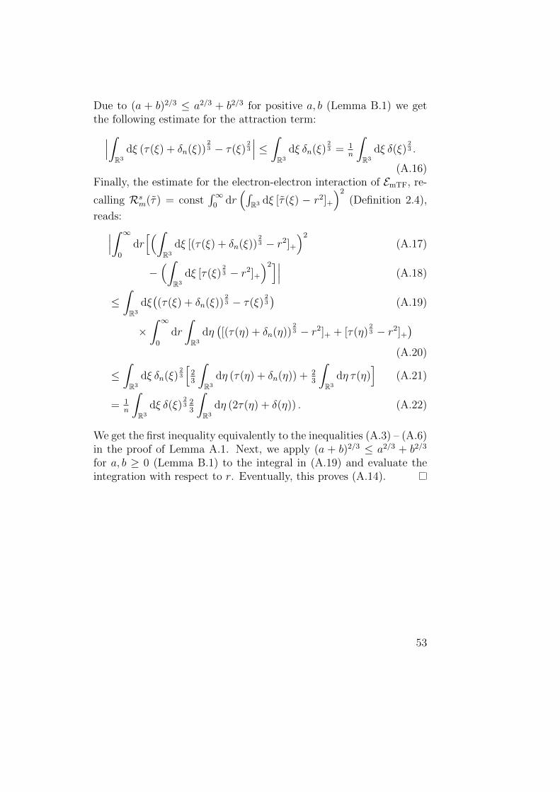
EmTF(τ + δn)− EmTF(τ) < const 1n. (A.14)

In fact, this shows that if N increases, we may add δn arbitrarily closeto the origin by taking the limit n→∞. So, in order to prove (A.14),first note that

Km(τ + δn) = Km(τ) + 1n2Km(δ). (A.15)

52

Due to (a + b)2/3 ≤ a2/3 + b2/3 for positive a, b (Lemma B.1) we getthe following estimate for the attraction term:∣∣∣∫

R3

dξ (τ(ξ) + δn(ξ))23 − τ(ξ)

23

∣∣∣ ≤ ∫R3

dξ δn(ξ)23 = 1

n

∫R3

dξ δ(ξ)23 .

(A.16)Finally, the estimate for the electron-electron interaction of EmTF, re-

calling Rsm(τ) = const

∫∞0

dr(∫

R3 dξ [τ(ξ) − r2]+

)2(Definition 2.4),

reads:∣∣∣∫ ∞0

dr[(∫

R3

dξ [(τ(ξ) + δn(ξ))23 − r2]+

)2(A.17)

−(∫

R3

dξ [τ(ξ)23 − r2]+

)2]∣∣∣ (A.18)

≤∫R3

dξ((τ(ξ) + δn(ξ))

23 − τ(ξ)

23

)(A.19)

×∫ ∞0

dr

∫R3

dη([(τ(η) + δn(η))

23 − r2]+ + [τ(η)

23 − r2]+

)(A.20)

≤∫R3

dξ δn(ξ)23

[23

∫R3

dη (τ(η) + δn(η)) + 23

∫R3

dη τ(η)]

(A.21)

= 1n

∫R3

dξ δ(ξ)23 23

∫R3

dη (2τ(η) + δ(η)) . (A.22)

We get the first inequality equivalently to the inequalities (A.3) – (A.6)in the proof of Lemma A.1. Next, we apply (a + b)2/3 ≤ a2/3 + b2/3

for a, b ≥ 0 (Lemma B.1) to the integral in (A.19) and evaluate theintegration with respect to r. Eventually, this proves (A.14).

53

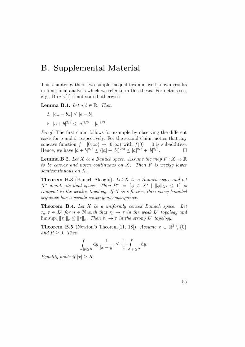
B. Supplemental Material

This chapter gathers two simple inequalities and well-known resultsin functional analysis which we refer to in this thesis. For details see,e. g., Brezis [1] if not stated otherwise.

Lemma B.1. Let a, b ∈ R. Then

1. |a+ − b+| ≤ |a− b|.

2. |a+ b|2/3 ≤ |a|2/3 + |b|2/3.

Proof. The first claim follows for example by observing the differentcases for a and b, respectively. For the second claim, notice that anyconcave function f : [0,∞) → [0,∞) with f(0) = 0 is subadditive.Hence, we have |a+ b|2/3 ≤ (|a|+ |b|)2/3 ≤ |a|2/3 + |b|2/3.

Lemma B.2. Let X be a Banach space. Assume the map F : X → Rto be convex and norm continuous on X. Then F is weakly lowersemicontinuous on X.

Theorem B.3 (Banach-Alaoglu). Let X be a Banach space and letX∗ denote its dual space. Then B∗ := {φ ∈ X∗ | ‖φ‖X∗ ≤ 1} iscompact in the weak-∗-topology. If X is reflexive, then every boundedsequence has a weakly convergent subsequence.

Theorem B.4. Let X be a uniformly convex Banach space. Letτn, τ ∈ Lp for n ∈ N such that τn → τ in the weak Lp topology andlim supn ‖τn‖p ≤ ‖τ‖p. Then τn → τ in the strong Lp topology.

Theorem B.5 (Newton’s Theorem [11, 18]). Assume x ∈ R3 \ {0}and R ≥ 0. Then ∫

|y|≤Rdy

1

|x− y|≤ 1

|x|

∫|y|≤R

dy.

Equality holds if |x| ≥ R.

55

Bibliography

[1] Haim Brezis. Functional Analysis, Sobolev Spaces and PartialDifferential Equations. Universitext. Springer, 2011.

[2] Marek Cinal and Berthold-Georg Englert. Thomas-Fermi-Scottmodel in momentum space. Phys. Rev. A, 45:135–139, Jan 1992.

[3] Berthold-Georg Englert. Energy functionals and the Thomas-Fermi model in momentum space. Phys. Rev. A, 45:127–134, Jan1992.

[4] Laszlo Erdos and Jan Philip Solovej. Semiclassical eigenvalueestimates for the Pauli operator with strong non-homogeneousmagnetic fields. II. Leading order asymptotic estimates. Comm.Math. Phys., 188(3):599–656, 1997.

[5] Laszlo Erdos and Jan Philip Solovej. Ground state energy oflarge atoms in a self-generated magnetic field. Communicationsin Mathematical Physics, 294(1):229–249, 2010.

[6] Enrico Fermi. Un metodo statistico per la determinazionedi alcune proprieta dell’atomo. Atti della Reale AccademiaNazionale dei Lincei, Rendiconti, Classe di Scienze Fisiche,Matematiche e Naturali, 6(12):602–607, 1927.

[7] Enrico Fermi. Eine statistische Methode zur Bestimmung einigerEigenschaften des Atoms und ihre Anwendungen auf die Theoriedes periodischen Systems der Elemente. Z. Phys., 48:73–79, 1928.

[8] Wilhelm Lenz. Uber die Anwendbarkeit der statistischen Metho-de auf Ionengitter. Z. Phys., 77:713–721, 1932.

[9] Elliott H. Lieb. A lower bound for Coulomb energies. Phys. Lett.,70A:444–446, 1979.

57

[10] Elliott H. Lieb. Thomas-fermi and related theories of atoms andmolecules. Rev. Mod. Phys., 53(4):603–641, October 1981.

[11] Elliott H. Lieb and Michael Loss. Analysis, volume 14 of Grad-uate Studies in Mathematics. American Mathematical Society,Providence, RI, second edition, 2001.

[12] Elliott H. Lieb and Barry Simon. Thomas-Fermi Theory Revis-ited. Physical Review Letters, 31(11):681–683, 1973.

[13] Elliott H. Lieb and Barry Simon. The Thomas-Fermi Theory ofAtoms, Molecules and Solids. Adv. Math., 23:22–116, 1977.

[14] Elliott H. Lieb, Jan Philip Solovej, and Jakob Yngvason. Asymp-totics of heavy atoms in high magnetic fields: I. Lowest landauband regions. Communications on Pure and Applied Mathemat-ics, 47(4):513–591, 1994.

[15] Elliott H. Lieb, Jan Philip Solovej, and Jakob Yngvason. Asymp-totics of heavy atoms in high magnetic fields. II. Semiclassicalregions. Comm. Math. Phys., 161(1):77–124, 1994.

[16] Elliott H. Lieb and Walter E. Thirring. Bound for the kineticenergy of Fermions which proves the stability of matter. Phys.Rev. Lett., 35(11):687–689, September 1975. Erratum: Phys. Rev.Lett., 35(16):1116, October 1975.

[17] Elliott H. Lieb and Walter E. Thirring. Inequalities for the mo-ments of the eigenvalues of the Schrodinger Hamiltonian and theirrelation to Sobolev inequalities. In Elliott H. Lieb, Barry Si-mon, and Arthur S. Wightman, editors, Studies in MathematicalPhysics: Essays in Honor of Valentine Bargmann. Princeton Uni-versity Press, Princeton, 1976.

[18] Isaac Newton. Philosophiae naturalis principia mathematica. Vol.I. Harvard University Press, Cambridge, Mass., 1972. Reprintingof the third edition (1726) with variant readings.

[19] Erwin Schrodinger. Der stetige Ubergang von der Mikro- zurMakromechanik. Naturwissenschaften, 14(28):664–666, 1926.

58

[20] Heinz Siedentop and Rudi Weikard. On the leading energy cor-rection for the statistical model of the atom: Interacting case.Comm. Math. Phys., 112:471–490, 1987.

[21] Heinz Siedentop and Rudi Weikard. Upper bound on the groundstate energy of atoms that proves Scott’s conjecture. Phys. Lett.A, 120:341–342, 1987.

[22] Heinz Siedentop and Rudi Weikard. On the leading energy correc-tion of the statistical atom: Lower bound. Europhysics Letters,6:189–192, 1988.

[23] Heinz Siedentop and Rudi Weikard. On the leading correction ofthe Thomas-Fermi model: Lower bound – with an appendix byA. M. K. Muller. Invent. Math., 97:159–193, 1989.

[24] Heinz Siedentop and Rudi Weikard. A new phase space localiza-tion technique with application to the sum of negative eigenvaluesof Schrodinger operators. Annales Scientifiques de l’Ecole Nor-male Superieure, 24(2):215–225, 1991.

[25] Arnold Sommerfeld. Asymptotische Integration der Differential-gleichung des Thomas-Fermischen Atoms. Z. Phys. A, 78:283–308, 1932.

[26] Llewellyn H. Thomas. The calculation of atomic fields. Proc.Camb. Phil. Soc., 23:542–548, 1927.

[27] Verena von Conta and Heinz Siedentop. Statistical Theory ofthe Atom in Momentum Space. Markov Processes and RelatedFields, to appear, arXiv:1108.1944v2, 2013.

59

Eidesstattliche Versicherung

(Siehe Promotionsordnung vom 12.07.2011, §8, Abs. 2 Pkt. 5)

Hiermit erklare ich an Eides statt, dass die hier vorliegende Disserta-tion von mir selbstandig ohne unerlaubte Beihilfe angefertigt wordenist.

Verena von Conta

Munchen, den 19.11.2014

Unterschrift Doktorand

Statistical Theory of the Atom in Momentum Space · STATISTICAL THEORY OF THE ATOM IN MOMENTUM...

Documents

Transcript of Statistical Theory of the Atom in Momentum Space · STATISTICAL THEORY OF THE ATOM IN MOMENTUM...