Statistical Process Control Approach to Reduce the ...

Statistical Process Control Approach to Reduce theBullwhip Effect

by

Harikumar IyerB.E. Mechanical Engineering, University of Poona, India, 1996

M.S. Mechanical Engineering, University of Massachusetts, Amherst, 2000

Saurabh PrasadB.E. Mechanical Engineering, Indian Railway Institute of Mechanical and Electrical

Engineering, 1993, Chartered Engineer (Institution of Engineers, India)

Submitted to the Engineering Systems Division in Partial Fulfillment of theRequirements for the Degree of

Master of Engineering in Logistics

at the

Massachusetts Institute of TechnologyJune 2007

0 2007H. Iyer and S. Prasad

All rights reserved

f ASACH-USET-IS INST7JTECEFCHNOLOGYsI EEfD

JUL 3 1 2007

LIBRARIES

The author hereby grants to MIT permission to reproduce and todistribute publicly paper and electronic copies of this thesis document in whole or in part.

Signature of Authors ........ .. c ..............................................Engineejing Systems Division

May 11, 2007

Certified by ......... ..............................................Chris Caplice

Executive Director, Master of Engineering in Lo istics//Thesis S rvisor

A ccepted b y ................................................................................ . ... . . .. .......... ..............ossi Sheffi

Professor of Civil and Environmental Engineering and Engi ering SystemsDirector, MIT Center for Transportation and Logistics

of 69

4VAOMWO10" 1110"I " -' -,

STATISTICAL PROCESS CONTROL APPROACH TOREDUCE THE BULLWHIP EFFECT

by

Harikumar Iyer and Saurabh Prasad

Submitted to the Engineering Systems Division on 5/11/2007 in partial fulfillment of the

requirements for the degree of Master of Engineering in Logistics

ABSTRACT

The bullwhip effect is a pervasive problem in multi echelon supply chains that

results in inefficient production operations and higher inventory levels. The causes of the

bullwhip effect are well understood in industry and academia. Quantitative and

qualitative solutions to attenuate this effect have been proposed in various research

studies. In this research a quantitative solution in the form of a Statistical Process Control

(SPC) based inventory management system is proposed that reduces the bullwhip effect

while reducing inventory without compromising service level requirements for a variety

of products. The strength of this methodology is in its effectiveness in reducing bullwhip

for fast moving products in the mature phase of their lifecycles where improving

production efficiency and lowering inventory investment are critical. However, fill rate

issues are observed for slow moving products and therefore, the methodology is not

recommended for such products. Finally, the application of this methodology to reduce

the bullwhip effect is illustrated for a product family of a medical devices company. The

results for the different classes of products in this family are discussed.

Thesis Advisor: Chris Caplice

Title: Executive Director, Master of Engineering in Logistics Program

of 69

ACKNOWLEDGEMENTS

I would like to thank Chris Caplice, Executive Director of the MLOG program

and our thesis advisor for his valuable guidance and support. I acknowledge my family

(in alphabetical order) - Anulekha, Belu, Dipali, Munni, Pista, Prashant, Shalabh, Shalin,

Mr. Sheo Shankar Prasad, Mrs. Shobha Prasad and Swati for their encouragement and

standing by me in their own different ways. I deeply appreciate Shalabh's support for

making my MIT studies a success. I would like to thank my classmates, and specially

Hari and his wife Olga who made my stay in Cambridge a cherished one.

This one's for Belu.

Saurabh Prasad

I am deeply grateful to Chris Caplice for teaching me the fundamental concepts

and theories used in this research and for his guidance and encouragement. I feel honored

to have worked with Saurabh on this thesis who weighed in on his rich experience and

thoughtfulness. I thank my wife, Olga, for her infinite patience and support as she juggled

her own academic commitments with the frequent flying schedules to meet me in Boston.

You are the best thing that happened to me. I owe my brother, Ramkumar, a special note

of appreciation for looking out for his younger brother. No one can make better tofu and

bean curry. I am thankful to the brightest minds in the MLOG class of 2007. I have learnt

much from you. Finally, none of my achievements would have been possible without the

moral and social values that my parents, R. Vijayan and Jamuna Vijayan inculcated in

me.

Harikumar Iyer

of 69

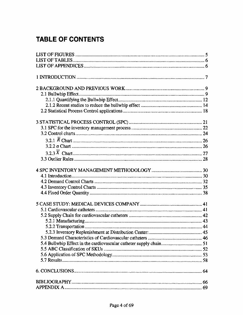
TABLE OF CONTENTS

LIST OF FIGURES ....................................................................................................... 5LIST OF TABLES .......................................................................................................... 6LIST OF APPENDICES................................................................................................ 6

1 INTRODUCTION ....................................................................................................... 7

2 BACKGROUND AND PREVIOUS WORK.............................................................. 92.1 Bullwhip Effect......................................................................................................... 9

2.1.1 Quantifying the Bullwhip Effect................................................................... 122.1.2 Recent studies to reduce the bullwhip effect .............................................. 14

2.2 Statistical Process Control applications............................................................. 18

3 STATISTICAL PROCESS CONTROL (SPC)........................................................ 213.1 SPC for the inventory m anagem ent process ...................................................... 223.2 Control charts..................................................................................................... 24

3.2.1 Chart ............................................................................................................ 263.2.2 Chart ......................................................................................................... 26

3.2.3 Chart....................................................................................................... 273.3 Outlier Rules....................................................................................................... 28

4 SPC INVENTORY MANAGEMENT METHODOLOGY ...................................... 304.1 Introduction........................................................................................................ 304.2 Dem and Control Charts ...................................................................................... 324.3 Inventory Control Charts ................................................................................... 354.4 Fixed Order Quantity ........................................................................................... 38

5 CASE STUDY: MEDICAL DEVICES COMPANY............................................... 415.1 Cardiovascular catheters ................................................................................... 415.2 Supply Chain for cardiovascular catheters ........................................................ 42

5.2.1 M anufacturing.............................................................................................. 435.2.2 Transportation ............................................................................................. 445.2.3 Inventory Replenishment at Distribution Center:....................................... 45

5.3 Dem and Characteristics of Cardiovascular catheters ......................................... 465.4 Bullwhip Effect in the cardiovascular catheter supply chain.............................. 515.5 ABC Classification of SKUs .............................................................................. 525.6 Application of SPC M ethodology........................................................................ 535.7 Results..................................................................................................................... 58

6. CONCLUSIONS........................................................................................................ 64

BIBLIOGRAPHY .......................................................................................................... 66APPENDIX A ............................................................................................................... 69

of 69

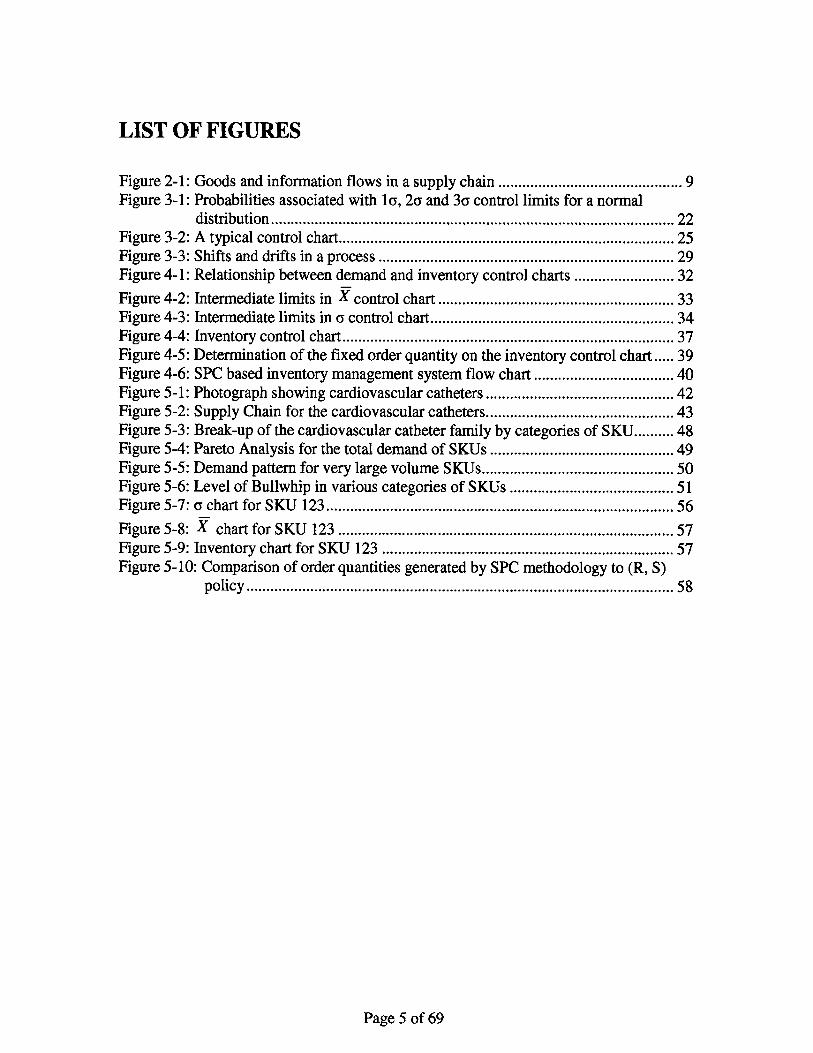
LIST OF FIGURES

Figure 2-1: Goods and information flows in a supply chain ......................................... 9Figure 3-1: Probabilities associated with lo, 2a and 3o control limits for a normal

distribution................................................................................................ 22Figure 3-2: A typical control chart............................................................................... 25Figure 3-3: Shifts and drifts in a process .................................................................... 29Figure 4-1: Relationship between demand and inventory control charts ..................... 32

Figure 4-2: Intermediate limits in X control chart ...................................................... 33Figure 4-3: Intermediate limits in a control chart......................................................... 34Figure 4-4: Inventory control chart............................................................................... 37Figure 4-5: Determination of the fixed order quantity on the inventory control chart..... 39Figure 4-6: SPC based inventory management system flow chart .............................. 40Figure 5-1: Photograph showing cardiovascular catheters ........................................... 42Figure 5-2: Supply Chain for the cardiovascular catheters.......................................... 43Figure 5-3: Break-up of the cardiovascular catheter family by categories of SKU.......... 48Figure 5-4: Pareto Analysis for the total demand of SKUs ......................................... 49Figure 5-5: Demand pattern for very large volume SKUs............................................ 50Figure 5-6: Level of Bullwhip in various categories of SKUs .................................... 51Figure 5-7: a chart for SKU 123................................................................................... 56

Figure 5-8: Y chart for SKU 123 ................................................................................ 57Figure 5-9: Inventory chart for SKU 123 .................................................................... 57Figure 5-10: Comparison of order quantities generated by SPC methodology to (R, S)

policy ..................................................................................................... . . 58

of 69

LIST OF TABLES

Table 2-1: A Framework for Supply Chain Coordination Initiatives ............................ 11Table 5-1: Transportation times in the manufacturer-distribution center echelon of

cardiovascular catheter supply chain........................................................ 44Table 5-2: Distribution of SKUs on the basis of volume sold...................................... 47Table 5-3: Demand variability characteristics of different categories of SKUs........... 49Table 5-4: SKUs in various categories having production smoothing ......................... 52Table 5-5: Characteristics of 'A', 'B', and 'C' classes of items of the cardiovascular

catheter fam ily .......................................................................................... 53Table 5-6: Reduction in levels of Bullwhip for 'A' class items with SPC based inventory

system compared to the present (R,S) inventory system........................... 59Table 5-7: Reduction in average inventory levels for 'A' class items with SPC based

inventory system compared to the present (R,S) inventory system........... 59Table 5-8: Reduction in levels of Bullwhip for 'B' class items with SPC based inventory

system compared to the present (R,S) inventory system........................... 60Table 5-9: Reduction in average inventory levels for 'B' class items with SPC based

inventory system compared to the present (R,S) inventory system........... 61Table 5-10: Bullwhip level for C Class SKUs with SPC based system ...................... 61Table 5-11: Break up of SKUs with increase in Bullwhip with SPC based system......... 62Table 5-12: Very small category SKUs showing an increase in bullwhip level .......... 62

LIST OF APPENDICES

APPEND IX A ................................................................................. 69

of 69

1 INTRODUCTION

The increase in demand variability as one moves upstream in the supply chain,

i.e., the 'Bullwhip effect', causes inefficient use of resources and higher supply chain

costs. These costs are due to higher inventory being stocked and transported to meet the

target customer service levels. Strategies to reduce the bullwhip effect and thus inventory

levels include information sharing, channel alignment and improvement of operational

efficiencies that are used by industries with varying degrees of success. The continued

focus on improving efficiencies and reducing costs leads researchers to explore newer

concepts and different techniques to improve supply chains. This research applies the

Statistical Process Control (SPC) principles, primarily used to monitor process variations

in manufacturing, to the field of supply chain management. Specifically, the SPC

principles shall be applied to develop an inventory management technique and assess its

impact in reducing the Bullwhip effect.

This thesis addresses the question as to whether the principles of SPC can be

applied to better manage inventory held at a distribution center and level load the

upstream production facility in order to reduce the bullwhip effect and lower the overall

supply chain costs.

SPC is used extensively in manufacturing. By establishing an upper and lower

bound on a process, such as manufacturing, one can determine if the process is within or

outside of normal operating conditions. This research examines if the inventory

management technique based on SPC principles can be used within the replenishment

of 69

cycle. This would entail establishing a statistically valid range by defining upper and

lower control limits instead of having standard point replenishment. The thought is that

this will allow us to dampen the over-reactions that can cause the bullwhip effect. Using

research and modeling, the project would demonstrate how the principles of SPC can

impact the inventory at a distribution center and the inventory replenishment planning at

the manufacturing facility. As a part of the research case study, the SPC approach shall

be compared against current inventory and replenishment policies at a medical device

company.

In the following chapter, literature pertinent to the bullwhip effect, its causes and

resolution strategies are reviewed. Chapter 3 introduces Statistical Process Control

concepts which are applied to develop an inventory management methodology in Chapter

4. The methodology is demonstrated for a medical devices company in Chapter 5 and the

results are discussed. Finally, in Chapter 6, the strengths and limitations of this SPC-

based inventory management system are summarized and recommendations for further

research are made.

of 69

2 BACKGROUND AND PREVIOUS WORK

Metters (1997) describes a typical supply chain for creation and sale of goods that

involves distinct echelons operating in a serial time-line (Figure 2-1). In such a typical

supply chain suppliers provide raw materials to manufacturers, who process the raw

materials into finished goods and then provide the finished goods to wholesalers who

combine products from a number of manufacturers for sale to retailers, who then sell the

product to the consumer. In addition to the physical flow of goods downstream in the

chain, there is an information flow that proceeds upstream. The retailer has direct contact

with the ultimate consumer who is at the end of the supply chain. The demand seen by

wholesalers consists of orders from retailers, rather than consumers, and so on for

upstream entities of the supply chain. The goods and information flows in a supply chain

can be shown in Figure 2-1.

Flow of Physical Goods

Supplier Manufacturer Wholesaler Retailer

Flow of Demand Information

Figure 2-1: Goods and information flows in a supply chain

2.1 Bullwhip Effect

Demand variability increases as we move up the supply chain. This phenomenon

is called the Bullwhip Effect. Lee, Padmanabhan and Whang (1997a) state that the

of 69

Bullwhip effect exists when the orders to the supplier tend to have larger variance than

sales to the buyer (i.e. demand distortion). Also, this distortion propagates upstream in an

amplified form (i.e. variance amplification). The costs for this variability are - inefficient

use of production and warehouse resources, higher transportation costs, and high

inventory costs (Silver, Pyke and Peterson, 1998). In order to reduce such costs,

companies make efforts to improve supply chain management aimed by reducing the

bullwhip effect.

Lee, Padmanabhan, and Whang (1997b) identify four rational factors that create

the bullwhip effect.

1 Demand signal processing: In case the demand increases, firms order more in

anticipation of further increases, thereby communicating an artificially higher level of

demand.

2 The rationing game: To obviate possible shortages, firms order more than the actual

forecast in anticipation of receiving a larger share of the items in short supply.

3 Order batching: Fixed costs at one location lead to batching of orders

4 Manufacturer price variations: Volume based discounts encourage bulk orders.

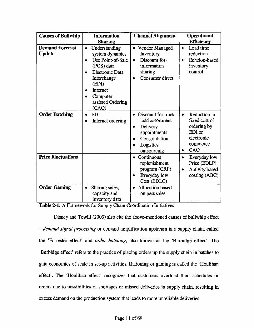
Lee et al (1997b) further suggest information sharing amongst supply chain

partners, channel alignment and improving operational efficiencies as the three broad

strategies to reduce the bullwhip effect in the supply chain. Their framework, which

includes the different types of initiatives that can be made by the supply chain members,

is shown in Table 2-1.

of 69

Causes of Bullwhip Information Channel Alignment OperationalSharing Efficiency

Demand Forecast * Understanding e Vendor Managed * Lead timeUpdate system dynamics Inventory reduction

* Use Point-of-Sale 9 Discount for * Echelon-based(POS) data information inventory

* Electronic Data sharing controlInterchange e Consumer direct(EDI)

* Internet* Computer

assisted Ordering(CAO)

Order Batching * EDI e Discount for truck- * Reduction in* Internet ordering load assortment fixed cost of

e Delivery ordering byappointments EDI or

* Consolidation electronic

o Logistics commerceoutsourcing * CAO

Price Fluctuations o Continuous * Everyday lowreplenishment Price (EDLP)program (CRP) * Activity based

* Everyday low costing (ABC)Cost (EDLC)

Order Gaming * Sharing sales, * Allocation basedcapacity and on past salesinventory data

Table 2-1: A Framework for Supply Chain Coordination Initiatives

Disney and Towill (2003) also cite the above-mentioned causes of bullwhip effect

- demand signal processing or demand amplification upstream in a supply chain, called

the 'Forrester effect' and order batching, also known as the 'Burbidge effect'. The

'Burbidge effect' refers to the practice of placing orders up the supply chain in batches to

gain economies of scale in set-up activities. Rationing or gaming is called the 'Houlihan

effect'. The 'Houlihan effect' recognizes that customers overload their schedules or

orders due to possibilities of shortages or missed deliveries in supply chain, resulting in

excess demand on the production system that leads to more unreliable deliveries.

of 69

2.1.1 Quantifying the Bullwhip Effect

Chen, Drezner, Ryan and Simchi-Levi (2000), quantify the bullwhip effect in

terms of the variance of the orders placed by the retailer to the manufacturer relative to

the variance of the demand faced by the retailer. They consider a simple two echelon

supply chain comprising a single manufacturer and a single retailer, having an order up-to

policy. They quantify the Bullwhip in terms of the order and demand variances (Equation

2-1).

52Bullwhip =-f-. Equation (2-1)

(D

where U denotes variance of orders q, and U2 is the variance of demand D.

Disney, Towill and van de Velde (2004), also use this metric as a measure of

Bullwhip, and give it the name 'Variance Ratio'. They further state that Variance Ratio >

1 results in a bullwhip; Variance Ratio < 1 results in order smoothing; and Variance Ratio

= 1 may result in a "pass-on-orders" policy, where the production pattern exactly

follows the demand pattern. This metric can be applied to a single ordering decision or

echelon in a supply chain (Disney and Towill, 2003) or across many echelons in the

supply chain (Dejonckheere et al, 2004). In the case where Variance ratio < 1 or order

smoothing, a firm might not be able to meet its customer service levels when faced with

increase in demand due to variability. In case the firm produces large quantities to

smooth its production, the inventory levels would increase due to larger safety stocks in

the supply chain to meet the same customer service levels.

Another metric to measure the Bullwhip Effect has been in terms of the

of 69

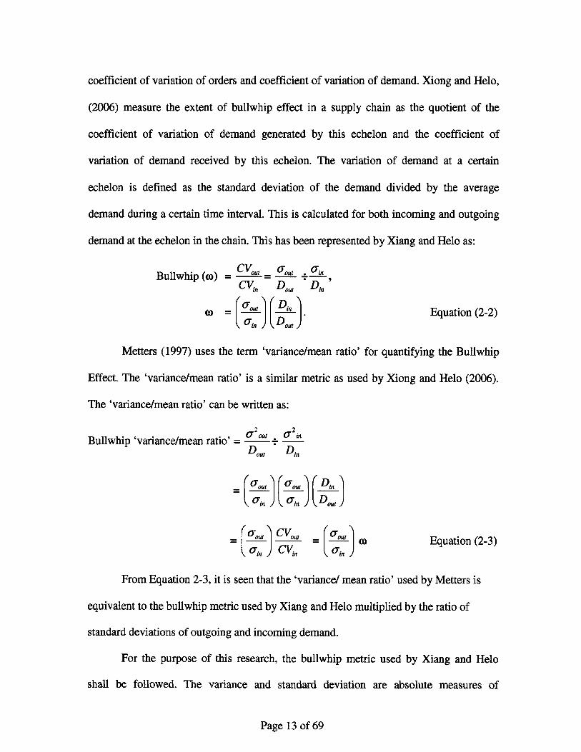
coefficient of variation of orders and coefficient of variation of demand. Xiong and Helo,

(2006) measure the extent of bullwhip effect in a supply chain as the quotient of the

coefficient of variation of demand generated by this echelon and the coefficient of

variation of demand received by this echelon. The variation of demand at a certain

echelon is defined as the standard deviation of the demand divided by the average

demand during a certain time interval. This is calculated for both incoming and outgoing

demand at the echelon in the chain. This has been represented by Xiang and Helo as:

Bullwhip (w) = "'= -- +CVn Du Din

0 = ""' . Equation (2-2)cin xDo

Metters (1997) uses the term 'variance/mean ratio' for quantifying the Bullwhip

Effect. The 'variance/mean ratio' is a similar metric as used by Xiong and Helo (2006).

The 'variance/mean ratio' can be written as:

2 2

Bullwhip 'variance/mean ratio' = 0 out + 'nDout Di

=( out ( out Dill__

= t CV- " = "o' ) Equation (2-3)a CVn a

From Equation 2-3, it is seen that the 'variance/ mean ratio' used by Metters is

equivalent to the bullwhip metric used by Xiang and Helo multiplied by the ratio of

standard deviations of outgoing and incoming demand.

For the purpose of this research, the bullwhip metric used by Xiang and Helo

shall be followed. The variance and standard deviation are absolute measures of

of 69

dispersion, depending upon the units of measurement. Coefficient of variation is a

relative measure of dispersion and is a pure number independent of units of measurement.

It is therefore more suitable for comparing the variability of two distributions (Gupta,

1992). The variability of the distribution of outgoing demand can be compared with the

distribution of incoming demand at an echelon and the distribution with a lower

coefficient of variation is considered to be less variable (or more homogenous) than the

other.

2.1.2 Recent studies to reduce the bullwhip effect

Significant research has been done in the last ten years on the topic of reducing

the bullwhip effect using the above mentioned framework. The research ranged from

evaluating the information sharing strategy, to vendor managed inventory as a channel

alignment strategy, and to improving operational efficiencies using various approaches

like fuzzy sets theory, non-linear goal programming, integrated production-inventory

models etc. An overview of some of the recent research studies on the subject is as under.

Information sharing strategies

Lee, Padmanabhan, and Whang (1997b) state that the information transferred in

the form of orders tends to be distorted and can misguide upstream members in their

inventory and production decisions. Information sharing strategies to reduce the bullwhip

effect has been one of the most researched topics in the area of bullwhip effect. Lau et al

(2003) researches the impacts of sharing information on the supply chain dynamics, and

reviews recent representative papers since 1996. Their review shows that the benefits of

information sharing are significant in reducing the bullwhip effect as supply chain entities

of 69

can make better decisions on ordering, capacity allocation and production/material

planning for optimizing supply chain dynamics.

Wong et al (2007) compares actual bullwhip effects provided by retailers who

shared downstream demand information and retailers who did not share demand

information in a three-echelon toy supply chain, A reduction in bullwhip effect and an

improvement of the fill rate was observed for retailers who shared downstream demand

information, to plan premature replenishment, and update forecast, even without

coordination between the toy manufacturer and the retailers.

Croson and Donohue (2006) studies the bullwhip effect from a behavioral

perspective in the context of a simple, serial, supply chain subject to information lags and

stochastic demand. They conduct two experiments on different sets of participants to find

that the bullwhip effect still exists when normal operational causes (e.g. batching etc.) are

removed. This was explained to some extent by evidence that decision-makers

consistently underweight the supply line when making order decisions. In the second

experiment, they found that the bullwhip, and the underlying tendency of

underweighting, remains when information on inventory levels is shared. However, the

information sharing helps somewhat to alleviate the bullwhip effect.

However, the trade-off between the costs of technology for information sharing and

the value generated by such investments, and lack of discipline in complying to the

collaborative process by supply chain partners, need to be addressed while adopting

information-sharing as the prime strategy to reduce the bullwhip effect. Lau et al (2003)

state that "information sharing, may not be beneficial to some supply chain entities due to

of 69

high adoption cost of joining the inter-organizational information system, unreliable and

imprecise information (Swaminathan et al., 1997; Cohen, 2000), and different operational

condition of each firm (Dong and Xu, 2001)."

Channel Alignment Strategies

Disney and Towill (2003) use a simulation model to compare the bullwhip effect in a

vendor managed inventory (VMI) supply chain with those of a traditional 'serially-

linked' supply chain. The model considers each of the four important sources of the

bullwhip effect in turn. The analysis shows that with VMI implementation two sources of

the bullwhip effect may be completely eliminated, i.e. rationing and gaming or the

Houlihan effect, and the order batching effect or the Burbidge effect. VMI is also

significantly better at responding to rogue changes in demand due to the promotion effect

or to price induced variations. However, the effect of VMI on demand signal processing

introduced bullwhip or the Forrester effect not clear. They state that VMI offers a

significant opportunity to reduce the bullwhip effect in real-world supply chains.

Operational efficiency strategies

Some research studies applied fuzzy sets theory in managing inventory strategies.

The most recent is of Xiong and Helo (2006). They cite Carlsson and Fuller (2001), who

proposed a fuzzy logic approach to reduce the bullwhip effect, and is used in the paper

industry. Xiong and Helo (2006) propose a multi-echelon fuzzy inventory model to

counteract the demand fluctuation in supply demand networks. By using a simulation

model, their research shows that the proposed multi-echelon fuzzy inventory model

of 69

provides can reduce the bullwhip effect with lower inventory levels and costs.

Dhahri and Chabchoub (2007) propose use of nonlinear goal programming

models as a decision making aid, by using preference functions based on a statistical

chronological series analysis (Box and Jenkins method) in order to construct the different

models for demand, stock level, and the order quantity. They further propose integration

of the decision maker preference in the demand forecast and inventory management

processes. Though results have not been encouraging, they have suggested the possibility

to integrate various statistical tools and mathematical models in a decision support system

for reduction in the inventory due to the bullwhip effect.

Boute et al (2007) suggest an integrated production and inventory model to

dampen upstream demand variability in the supply chain. They consider a two-echelon

supply chain, where the retailer would propagate demand variability often in amplified

form. The manufacturer, however, prefers to smooth production, and thus he prefers a

smooth order pattern from the retailer. At first sight, a decrease in order variability comes

at the cost of an increased variance of the retailer's inventory levels, inflating the

retailer's safety stock requirements. However, integrating the impact of the retailer's order

decision on the manufacturer's production leads to new insights. A smooth order pattern

generates shorter and less variable (production/replenishment) lead times, introducing a

compensating effect on the retailer's safety stock. It is shown in this research that by

including the impact of the order decision on lead times, the order pattern can be

smoothed to a considerable extent without increasing stock levels.

This thesis focuses on echelon based inventory control as a means to reduce the

bullwhip effect. The application of Statistical Process Control, a concept widely used in

of 69

the manufacturing environment especially for Quality Control, shall be explored to

inventory management policies and a simulation model shall be used to assess the impact

of such an approach on the bullwhip effect.

2.2 Statistical Process Control applications

Statistical quality control (SQC) dates back to the 1930s originating from the

work of Walter Shewart of Bell Telephone Laboratories. His student, W.Edwards

Deming, taught quality control in Japan, thereby igniting the Japanese quality revolution.

(Namhias, 2005). SQC generally focuses on manufacturing quality, as measured by

conformance to specifications. "The ultimate objective of SQC is the systematic

reduction of variability in quality measures. The three major classes of tools used in SQC

are Acceptance Sampling, Statistical Process Control (SPC), and Design of Experiments"

(Hopp and Spearman, 2000). In acceptance sampling, products are inspected to determine

whether they conform to specifications; while in SPC, processes are continuously

monitored with respect to mean and variability of performance to determine whether the

process is in control or has gone out of control. In Design of Experiments, causes of

quality problems are traced through specifically targeted experiments by varying

controllable variable to determine their effect on quality measures.

SPC has been primarily used in the manufacturing environment. However, the

possibility of using the SPC approach outside the manufacturing environment has also

been explored by various industries. For example, Jiang et al (2007) uses a SPC

framework to identify changes in business activity monitoring in telecommunications

industry for tracking diversified customer behaviors, to establish successful customer

of 69

loyalty programs for churn prevention and fraud detection. Health-care organizations use

SPC and six sigma to determine important elements of the healthcare experience to

consumers, and to monitor and reduce errors (e.g. medical errors, wait times, errors from

high-risk medications, turnaround time for pharmacy orders etc.) and their associated

costs (Camille James, 2006).

SPC has not been used much in the supply chain environment. This research aims

to extend the SPC technique beyond the manufacturing processes by applying it to the

inventory control area of supply chain management. By investigating its impact on the

level of bullwhip, this research fits into the strategy to improve operational efficiencies

for reducing the bullwhip effect.

A review of the literature indicates that SPC approach has been tried in inventory

management by the industry only to a very limited extent. SPC tools for specific forecast

periods were used by General Electric's aircraft engine division planners between 1993

and 1995, to reduce their aircraft engines parts inventory by 25% (Beck, 1999). The

demand forecast and inventory levels were monitored using control charts by comparing

statistic being monitored with applicable control limits, and placing any outlier on the

exception list for review. The use of specific forecast periods brought focus to apply the

SPC tools only where the application was successful during simulations.

Simulation studies using the SPC approach for management have been conducted

by Pfohl et al (1999) and Lee and Wu (2006). Pfohl et al (1999) uses data from 3M

Medical products for twelve European warehouses over a six month period. Decision

rules were set up for demand and inventory control charts to track changes in demand and

inventory. The average inventory levels reduced by 20% to 65%, but there were an

of 69

increase in back-orders for some products. However, the study was limited to examine

the effects on inventory levels by using the SPC approach.

Lee and Wu (2006) examine the bullwhip effect caused by order batching and

researched the traditional inventory replenishment method (event-triggered and time-

triggered inventory policies) and the SPC based replenishment method for a two echelon

supply chain. By using simulation, they find that the SPC method outperforms the

traditional methods in the categories of average inventory levels and, and in the number

of back-orders when the fill rate is 99%. However, at lower fill rate of 95%, the SPC

method reduces the back-orders but leads to higher inventory levels and increasing

variation in inventory levels.

SPC based inventory management systems have not focused on reducing the

bullwhip effect in supply chains. This thesis uses SPC to develop an inventory

management system as an operational strategy to control the amplification of demand

variability up the supply chain. In the following chapter, principles of statistical process

control are introduced that are later leveraged to develop the SPC based inventory

management system.

of 69

3 STATISTICAL PROCESS CONTROL (SPC)

Statistical process control offers a graphical means of monitoring a process in

real-time using control charts. Process variables are typically assumed to have an

underlying normal distribution. In the control charts, the process mean is represented by a

center line and the process standard deviation is captured in the upper and lower control

limits. A process is said to be in statistical control if it is within the control limits. Trends

in the process variable can be monitored real-time to identify deviations in the variable

from the historically calibrated state. The process supervisor can identify anomalies in a

process by monitoring the control charts. By conducting root-cause analysis, the

assignable causes for variation can be identified and resolved.

The Central Limit Theorem forms the basis of most control charts. The Central

Limit Theorem states that the distribution of the sum of independently and identically

distributed random variables approaches the Normal distribution as the number of terms

in the sum increases. In this light, the probability of having an observation of a process

variable outside controls limits can be easily determined. The probability associated with

finding an observation of a process variable that lies outside the 3y or -3Y control limits

on a control chart is less than 0.0026 or roughly less than 3 chances in 1,000. The

probabilities associated with finding observations outside la, 2T and 30 control limits are

shown in Figure 3-1.

of 69

15.87 87% 2.28% 2.28% 0.1 135%

-1 -10 r -2a -2 j.-3a -3a

Figure 3-1: Probabilities associated with lG, 2a and 3(y control limits for a normaldistribution

Since events involving observations that lie outside the 3y control limits are very

rare, a single event could signal an anomaly in the process that requires immediate

attention. However, events involving observations that lie between the 2y and 3y control

limits would require more than a single event to warrant remedial action. Events that

involve observations which lie between the center line and l and between lR and 2y are

higher probability events and therefore, require more a compelling case in terms of the

number of outliers to drive remedial action.

A process supervisor reacts to shifts and drifts in a process variable based on the

nature of the process involved. However, in general, a process supervisor would be

expected to investigate the causes for process deviation in the following manner:

1. Identify causes for the change in the process variable characteristics

2. Determine if the causes are endogenous to the system or exogenous

3. Effect remedial action for endogenous causes within the control of the process

supervisor

4. Coordinate with agents responsible for exogenous causes to mitigate operational

risk

3.1 SPC for the inventory management process

Inventory management is an emerging application for statistical process control in

of 69

which the key components of demand and inventory can be represented by control charts.

This requires the interpretation of demand and inventory to be the two tightly integrated

process variables for the inventory control process. Control charts can be created for each

of these variables based their historical characteristics. It will be demonstrated in

subsequent sections that the control charts for demand drives the control chart of

inventory. Once the control charts are created, subsequent observations of these variables

can be plotted on these charts to detect any situations where the variables are out of

control.

The use of SPC to manage demand and inventory has advantages over traditional

inventory management systems. Changes in demand characteristics, such as, the mean

and standard deviation measures of demand, drive inventory levels in the inventory

planning system. If these demand characteristics are updated frequently in the inventory

control system, the stocking requirements will also change resulting in system

nervousness. This would result in high production costs and inventory issues of deficits

or excesses. Therefore, it is critical to understanding whether the changes in demand

characteristics of a product are significant or not from an inventory planning perspective

before the inventory planning system is updated.

The following are the main advantages of using SPC in inventory management.

1. Develop greater understanding of the demand and inventory process variables and

recognize acceptable limits of operation

2. Determine when the demand and inventory process variables are out of control

3. Reduce nervousness in the ordering behavior by ensuring that changes are made

to the inventory system only when the process variables are out of control. This

of 69

significantly attenuate the bullwhip effect while maintaining service levels

The above advantages hold special merit for products that have low to moderate

volatility in demand (coefficient of variation of weekly demand less than 0.5). If minor

variations in the demand characteristics are passed on to the inventory planning system,

the fluctuations in the production orders can adversely impact the efficiency of the

production plant and result in greater production costs.

Once the changes in demand characteristics are transmitted to the inventory control

system, fluctuations in the order quantities to the production plant can be reduced

significantly by using economic order quantities (EOQ). However, the use of EOQ

requires that the demand be known with certainty and stay relatively constant throughout

the year which may not hold for many products. In such situations, the inventory chart

can be used to identify the fixed order quantity for the given state of demand. The

derivation of the fixed order quantity will be addressed in following sections. The fixed

order quantity obtained from the inventory chart for the given characteristics of demand

can reduce the production order variability and help level-load the production plant. The

predictability of a fixed order quantity for a given state of demand encourages habit

forming behavior in the production line and improves the efficiency of the production

process.

3.2 Control charts

Monitoring demand characteristics is directly relevant to inventory planning. A

change in mean demand results in changes in cycle inventory. A change in the standard

deviation of demand results in changes in safety stock levels. Therefore, demand needs to

of 69

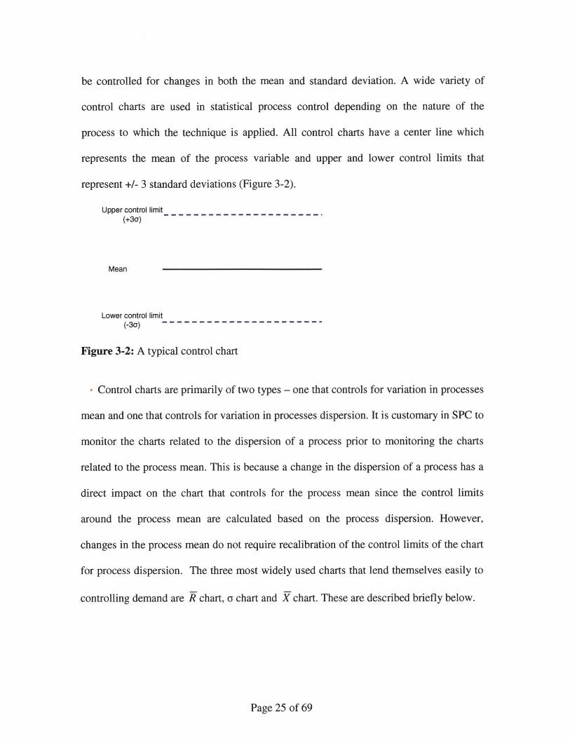
be controlled for changes in both the mean and standard deviation. A wide variety of

control charts are used in statistical process control depending on the nature of the

process to which the technique is applied. All control charts have a center line which

represents the mean of the process variable and upper and lower control limits that

represent +/- 3 standard deviations (Figure 3-2).

Upper control limit(+3a)

Mean

Lower control limit(-3a)- ----------------------

Figure 3-2: A typical control chart

- Control charts are primarily of two types - one that controls for variation in processes

mean and one that controls for variation in processes dispersion. It is customary in SPC to

monitor the charts related to the dispersion of a process prior to monitoring the charts

related to the process mean. This is because a change in the dispersion of a process has a

direct impact on the chart that controls for the process mean since the control limits

around the process mean are calculated based on the process dispersion. However,

changes in the process mean do not require recalibration of the control limits of the chart

for process dispersion. The three most widely used charts that lend themselves easily to

controlling demand are R chart, Y chart and X chart. These are described briefly below.

of 69

. ... .................... ............. ..... ..

3.2.1 R ChartAn k Chart controls for variation in process range. The popularity of the k chart

is historic. Prior to the advances in computation speed, k charts provided simplicity in

estimating the dispersion of a process. The range of a sample can be calculated with less

computational effort than the standard deviation. The average of the range of the samples

can be converted into an estimate of the standard deviation using the statistical

relationship between the mean range for data from a normal distribution and the standard

deviation of that distribution.

The center line of the chart can be constructed by calculating the range, Ri, for

each sample. The average of the sample ranges gives the center line, R. The upper and

lower control limits (UCL and LCL) for the chart can be computed using the factors of

D3 and D4 from the standard SPC/SQC table for k Charts (Appendix A). The values D3

and D4 are calculated based on the assumption of normal distribution and can be

determined for a given number of samples. The estimated standard deviation can be

computed from R by using the value d2 also from the standard SPC tables.

Ri LCL = D3 k UCL = D4 A=

n Id2

k charts are best suited for samples sizes up to 10. For larger samples, the

k statistic becomes a poor estimator of the sample standard deviation. For these sample

sizes the a chart become a more appropriate chart for controlling process dispersion.

3.2.2 a ChartThe a Chart controls for variation in process standard deviation. Computing the

of 69

standard deviation of samples has historically been computationally more intensive.

However, the level of effort to generate a Chart has been greatly eased with the

development of higher computing capabilities.

The center line of the chart can be constructed by calculating the standard

deviation, si, for each sample. The average of the sample standard deviations gives the

center line, Y and represents the estimated standard deviation for the process. The upper

and lower control limits (UCL and LCL) for the chart can be computed using the values

of B3 and B4 from the standard SPC/SQC table (Appendix A).

I nS= si LCL = B3 3 UCL = B4 3

nlI

a Charts are best suited for larger number of samples of 10 and greater. For sample sizes

between 6 and 10 the accuracy of using the k Chart decrease to less than 90% compared

to the a Chart decreases, making the a Chart a better suited candidate (Jack Prins, 2003).

For the purposes of this research, the a Chart is chosen over the k Chart to

control for standard deviation of demand due to the larger sample sizes (6 to 12) used in

the methodology. The details of this methodology are provided in the next chapter.

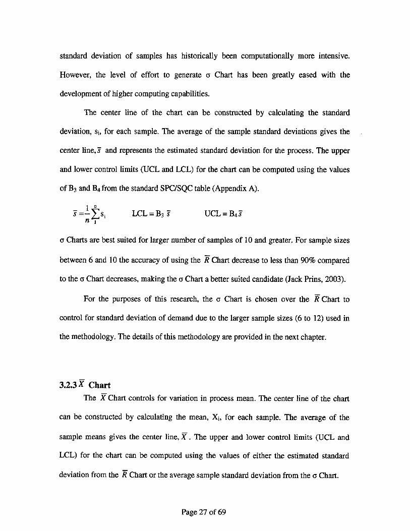
3.2.3 ChartThe X Chart controls for variation in process mean. The center line of the chart

can be constructed by calculating the mean, X, for each sample. The average of the

sample means gives the center line, X . The upper and lower control limits (UCL and

LCL) for the chart can be computed using the values of either the estimated standard

deviation from the k Chart or the average sample standard deviation from the a Chart.

of 69

1 nx - x

LCL= Y +3.Y UCL= Y -3.S for a Chart

where, T represents the average of the sample standard deviations from the aChart

LCL= Y +3.a UCL= Y -3.6 for RChart

where, a represents the estimate of the standard deviation from the k Chart

3.3 Outlier Rules

For the purposes of this document, two types of statistically out of control

situations are defined. A shift in a process refers to the a situation in which the process is

deemed out of control due to observations on a control chart that are consistently beyond

the 2y control limits above and below the center line. This includes observations that are

2a to oo and -2F to - oo on the control chart. A drift in a process refers to the situation in

which the process is deemed out of control due to consecutive observations on a control

chart that are between the center line and +2a and between the center line and -2G.

Essentially, a shift is a higher magnitude event than a drift. A shift may represent the

addition or removal of a customer. On the other hand, a drift may represent a steady

growth in demand from an existing customer. Shifts and drifts are shown in the figure 3-3

below.

of 69

+3s

+2s

+Isn

0.. .. .... ....

ProcessShift

Ms

-3s

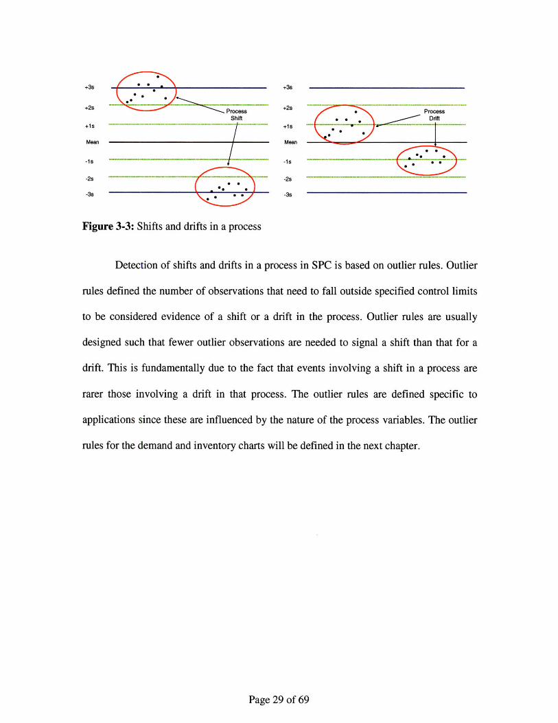
Figure 3-3: Shifts and drifts in a process

+2s

+Is

Mean

-is

-2s

-3s

Detection of shifts and drifts in a process in SPC is based on outlier rules. Outlier

rules defined the number of observations that need to fall outside specified control limits

to be considered evidence of a shift or a drift in the process. Outlier rules are usually

designed such that fewer outlier observations are needed to signal a shift than that for a

drift. This is fundamentally due to the fact that events involving a shift in a process are

rarer those involving a drift in that process. The outlier rules are defined specific to

applications since these are influenced by the nature of the process variables. The outlier

rules for the demand and inventory charts will be defined in the next chapter.

of 69

.................. ..... ............... I ... .. ............................. ..................Process

Drift.......... ............. V ............ . ......... ..................... ............. ......

................ I .................... ..................... ...... ...... .... 'i ...... ......

................................................................. .................. ................ .........

.......... I ....................... ................................................... I ....................

4 SPC INVENTORY MANAGEMENT METHODOLOGY

4.1 IntroductionThe inventory management methodology developed as part of this research

applies statistical process control techniques to traditional inventory management. In

particular, a basic inventory policy with periodic review, (R, S) policy, is enhanced with

control charts for managing demand and inventory levels to adapt the reorder point and

order quantities to reduce the bullwhip effect while simultaneously maintaining or

reducing inventory levels without any degradation in service levels.

In the (R, S) policy, for an inventory review period of R and a order lead time of

L, the order up to level, S can be computed as below.

S=XL +kOkLR Equation (4-1)

where, XL is the demand over the lead time and kaL,,R represents the safety

stock. Here, k is the safety stock factor and oJL+R is the standard deviation of

demand over the sum of the review period and lead time

The order quantity in this policy is determined as the difference between the order up to

level and the inventory level at a review period. The order quantity will change from

period to period if the demand is non-stationary. Further, the order up to level, S, may

itself need to be monitored and recomputed if the demand characteristics change. From

Equation 4-1, it is clear that a change in the demand characteristics will impact either the

cycle stock or safety stock requirements or both. Company typically periodically review

trends in demand and update the mean and standard deviation of demand in their

inventory systems.

of 69

The (R, S) policy described above is modified by incorporating SPC techniques to

create an integrated demand and inventory planning system that monitors and responds to

shifts and drifts in demand characteristics and inventory levels. Consider a demand

process which operates in three states over time (Figure 4-1). In state 1, the demand

operates with a particular mean and standard deviation. In state 2, the standard deviation

increases due to higher volatility in demand. However, the mean demand remains steady

at the level at state 1. Finally, in state 3, the mean demand shifts to a new level and the

standard deviation decreases. The inventory control chart shows the operating limits of

the inventory process for each state of demand. From state 1 to state 2, it is seen that the

safety stock represented by the minimum inventory level increases due to the increase in

the standard deviation of the demand process. Similarly, the maximum inventory level

also shifts by the increase in the safety stock. The difference between the maximum

inventory level and the minimum inventory level represents the fixed order quantity of

the system. Clearly, the fixed order quantity remains unchanged from state 1 to state 2

and is purely a function of the mean demand. From state 2 to state 3, the mean demand

increases and the standard deviation of demand decreases. The inventory chart responds

by reducing the safety stock and increasing the fixed order quantity.

The ability of the system to monitor changes in demand characteristics and to

respond to such changes by recalculating the inventory and ordering requirements is

explained in detail in the following sections.

of 69

- __- Control limits

Mean level

0

t - Max inv. levelo -j O OQ OQ - Min inv. level

0I -Zero inv. level> OQ

0

State 1 State 2 State 3

Figure 4-1: Relationship between demand and inventory control charts

4.2 Demand Control ChartsAs described previously in Chapter 3, demand involves two important

parameters- mean and standard deviation. The X chart is used to control for the variation

in mean demand and the (Y chart is used to control for the variation in the standard

deviation of demand. The Xchart and a charts for demand are constructed using the

historical mean and standard deviation. Using historical demand for this purpose ensures

that the control charts are a good representation of the current state of demand. For the

purposes of this research, weekly demand is considered for the X and a charts.

Assume that 20 weeks of demand are used to construct the first estimate of the

Y chart and a charts. The total demand and standard deviation for each of the 20 weeks

can be computed. The average of the 20 weekly demand and standard deviation represent

the center lines on the X chart and a charts, respectively. The control limits are then

drawn around the center lines using the formulas below.

of 69

I n=- si LCL3 = B3 3 UCL3 = B4 S for Y Chart Eqn I

n

1=-$Xi LCL3= Y -3.T UCL3= Y + 3.Y for XChart Eqn 2nI

In addition to the outer control limits, intermediate controls limits are also drawn around

the center line that are 1 and 2 standard deviations above and below the center line. The

intermediate control limits for the X chart can be constructed by constructing UCL2 =

Y + 2. i, LCL2 =X - 2. I , UCLi = X + 1.Y and LCL1 = Y - 1.Y (Figure 4-2).

However, for the a Chart, LCL2 is calculated to be such that it is a third of the distance

between the center line and LCL3 from LCL3 in the direction of the center line. LCLl is

midway between LCL2 and the center line (Figure 4-3).

UCL3 ------.--

UCL2 --...---------------- ....---------- ....-.-..---.-..----- ..-.-.------- .....----.....---- ...-- ..- - --

UCL1 .-... ... ........... ..... ...... ... ................. +2a

L O Ul . . . . . . . . . ... ......................I.. . . . . . . . . . . . . . . . . . . . . . . . . . . . . . . . -2 a-3

LCL2 ....................................................................... LL C L 1 -- -..-- - -- -..--- -- - - - -.. ~~ - - -I- -2-- --

LCL3 - ---ch-r-

Figure 4-2: Intermediate limits in X control chart

of 69

UCL3

UCL2 .- --

UCL1 ............................................ +2(UCL3 - s-bar)/3

+(UCL3 - s-bar)/3

s-bar

-(UCL3 - s-bar)/3

LC.L/............................................-2(s-bar - LCL3)/3

LC L2 ..-- .--- - ------- - - ------------------ - ---. - -- ---.-. -

LCL3

Figure 4-3: Intermediate limits in cY control chart

Once the demand control charts are created, outlier rules are defined. The outlier rules

ensure that sufficient data exists to signal a change in the process characteristics. The

following is an example of a set of outlier rules where an out of control event is signaled:

1. If a single observation exists above +3 Y limits

2. If two consecutive observations exist above the +2 c limits

3. If six consecutive observations exist above the +1 c limits

4. If twelve consecutive observations exist above the center line

Similar rules can also be defined for observations that lie below the center line.

Now, new observations of mean demand and standard deviation of demand are collected.

Consider a window of 10 weeks over which observations are collected. The weekly

demand over the most recent 10 weeks would be treated as the current week's mean

demand observation. Also, the weekly standard deviation of the most recent 10 weeks

would be treated as the current week's standard deviation observation. Once this data is

compiled, the standard deviation observation is first entered on the (T Chart. If the

observation satisfies an outlier rule, the c Chart indicates an out of control process. The

of 69

process supervisor is alerted and the system recommends that the center line of the a

chart, Y, be adjusted. The adjustment may be calculated by averaging a specified number

of the most recent observations. The center line and the corresponding control limits of

the a chart are now updated.

The a chart directly impacts the control limits of the X chart. If the a chart

changes, so will the X chart. The X chart is updated to reflect the appropriate control

limits. Now the mean demand observation for the current week is entered on the X chart

and tested for the outlier rules for the X chart. If the outlier rules are satisfied, the

Y chart signals an out of control event. The process supervisor is alerted and the system

recommends that the center line of the X chart, X, be adjusted. The adjustment may be

calculated by averaging a specified number of the most recent observations. The center

line and the corresponding control limits of the X chart are now updated.

In the event that none of the outlier rules are satisfied, the X chart and a chart are

maintained as per their current state.

4.3 Inventory Control Charts

Once the demand control charts are constructed, the inventory control chart can

be derived. The inventory control chart recommended in this research is the X chart and

is constructed for the average minimum inventory level (safety stock level). The

minimum inventory level can be calculated from the standard deviation of demand for a

given level of service. For a product with standard deviation of demand a with a lead

of 69

time L, review period R and a customer service safety factor k on the (R, S) policy, the

safety stock can be computed as follows.

SS=kaL+R

where, uL+R is the standard deviation of demand over L + R

The safety stock represents the average minimum level of inventory as the center line of

the X chart. To determine the control limits around the center line, the standard deviation

of the inventory around safety stock first needs to be calculated. Consider figure 4-4 that

shows a sample plot of inventory over a period in time with a characteristic saw tooth

profile using the (R, S) policy. The steep vertical lines represent inflow of inventory

while the lines with the slopes indicate the consumption of inventory at some rate. In

each cycle, the inventory hits a lowest point which on an average is the safety stock. The

lowest point inventory in a cycle can be expressed as follows:

I-= S-DL+R

where, DL+R is the demand over L + R and S is the reorder point for the policy

Since the S is a constant for a given state of demand, the variability in I- is the

variability in the demand over the lead time and review period. Intuitively, this is the

same standard deviation used in the computation of the safety stock. With this

information, the inventory control chart can be constructed (Figure 4-4). The chart is

constructed only with +1 oL+R and-' UL+R control limits.

of 69

1+

I-(safetystock)

Zeroinv.

Figure 4-4: Inventory control chart

The inventory control chart is used as a feedback correction mechanism to

augment orders placed by the SPC inventory system if the inventory falls below the lower

control limit on the chart. The ability of the system to anticipate potential shortages of

inventory improves over all fill rates as compared to the standard (R, S) policy. The

inventory chart only includes the minimum inventory level to ensure that the required

customer service is met. The need for the maximum inventory level is obviated by the

intelligence of the system to compute a fixed order quantity described in the following

section.

It is important to note here that since the inventory control chart is derived from

the parameters on the demand control charts, a change in the demand control chart will

cascade changes into the inventory control chart.

of 69

4.4 Fixed Order Quantity

For a production plant, achieving a fixed quantity of supply that meets customer

demand is beneficial for various reasons. The pattern of fixed production quantities result

in a habit forming schedule for the plant. The schedule of a fixed production quantity for

a product improves efficiencies of production with implications to lowering the cost of

production. However, the recommended fixed order quantity for a state of demand must

be such that it does not negatively impact inventory investment and the fill rate. The

methodology assumes that the fill rate is an adequate measure of customer satisfaction.

The SPC inventory management system has the ability to determine a fixed order

quantity for a given level of demand based on the characteristics of the (R, S) policy. The

average maximum inventory during each ordering cycle is expressed as below.

I+= S-DL

where, DL is the demand over lead time and S is the reorder point for the policy

The fixed order quantity (Figure 4-5) for a given demand is shown below.

Fixed Order Qty = I + - I -

The fixed order quantity is equivalent to the demand over review period for a given state

of demand on the control chart.

of 69

1+

oQ

F~+ 1 T .............-............................---- ..................................-----------.

- Max inv. level

F - Min inv. level

S- ................................................... ....................................... - Zero nv. levelSS

Figure 4-5: Determination of the fixed order quantity on the inventory control chart

If the (R, S) policy is simulated over a long duration, the average order quantity

placed by the (R, S) system will correspond to the fixed order quantity calculated above.

However, the order placed by the system will vary period over period. The fixed order

quantity calculated above may lead to excess and deficit inventory conditions in the short

term. The condition of deficit inventory would be the critical to business since this

represents lost sales or back orders with potential drop in customer service. However,

when the fixed order quantity logic is coupled with the inventory chart capability to

mitigate potential shortages by augmenting the order quantity, the quality of the plans the

system generates is improved. Further, the system places an order up to the new reorder

point for the first period when the reorder point changes.

It is important to note here that since the average maximum inventory level (I')

and the average minimum inventory level (I-) are derived from the parameters on the

demand control charts, a change in the demand control chart will cascade changes into

the inventory control chart and the estimate of the average maximum inventory level.

This will produce a change in the recommended fixed order quantity of the system.

of 69

Start (weekly)

Calculate rolling windowstandard deviation of

demand, 's'

Locate 's' on a chart

NoIs 's' anoutlier?

Yes

otir NoIs outlier Increment count of

rule outlierssatisfied?

Yes

Alter a chart, limits ofdemand X chart,

inventory X chart andfixed order qty

Calculate rolling windowmean demand, 'x'

Locate 'x' on demand Xchart

Nols 'x' anoutlier'?

Yes

Is outlier No Increment count ofrule outliers

Yes

Augment fixed order qtyAlter demand X chart, to adjust for anticipatedinventory X chart and stockout

fixed order qty

Locate current inv. on Is inv.inventory X chart -- an

(every review period) outlier?

Maintain fixed order qtyreplenishment

Figure 4-6: SPC based inventory management system flow chart

The flow chart presented in Figure 4-6 represents the robust framework for

controlling inventory developed in this section. Changes are made to inventory and

replenishment parameters only when statistically significant demand changes occur. In

this manner, demand signal processing effects based on speculation is minimized and the

system responsiveness is based on a set of well-defined rules. In the following section,

the methodology is applied to a product family of a medical devices company.

of 69

5 CASE STUDY: MEDICAL DEVICES COMPANY

Medical Devices Company is one of the world's leading developer and

manufacturer of breakthrough products for interventional medicine, minimally invasive

computer-based imaging, and electrophysiology for fighting disease. It sells products in

markets worldwide and is headquartered in the United States of America. Medical

Devices Company has five business units/divisions: cardiovascular disease management,

peripheral vascular and obstructive disease management, neurovascular management,

electrophysiology and medical sensor technology, and biologics delivery. The major

product families of the cardiovascular disease management division are Drug-eluting

stents, Guidewires, Cardiovascular catheters, Dilatation catheters, Sheath Introducers,

Biopsy forceps and Diagnostic Guidewires. This thesis studies the cardiovascular catheter

product family.

5.1 Cardiovascular catheters

The American Heart Association defines 'cardiac catheterization' as 'the process

of examining the heart by guiding a thin tube (catheter) into a vein or artery and passing

it into the heart and into the coronary arteries.' These tubes are called 'cardiovascular

catheters'. The cardiovascular catheters manufactured by Medical Devices Company are

tubes with stainless steel braiding, PTFE liner and a blended nylon outer coat. The

cardiovascular catheter is specified by both outer diameter (OD) and inner diameter (ID),

the length of the tip and shape of the catheter.

of 69

Figure 5-1: Photograph showing cardiovascular catheters

The cardiovascular catheter product family is in the mature phase of the product

life cycle. Though this product family has more than 500 Stock keeping units (SKU), the

case study shall be limited to those SKUs which fulfill the criterion that at least 20 weeks

of demand (orders placed by hospitals to the distribution center) history is available. This

has resulted in our analysis being limited to 397 SKUs.

5.2 Supply Chain for cardiovascular catheters

The supply chain for cardiovascular catheters is described in Figure 5-2. The

cardiovascular catheters are manufactured at a single location. After manufacturing, the

products are shipped to sterilization centers which hold inventory in the form of work-in-

progress (WIP). For the product to be sold in the Americas (comprising of United States

of America, Canada, Mexico, Latin America) catheters are transported to 'Location B'

for sterilization; and for the product to be sold in Europe, Asia, Africa and Australia, the

catheters are transported to 'Location D'. Subsequent to sterilization of the catheters, the

catheters are sent to the distribution centers which dispatch the products to customers as

per the demand. While the 'Location B' sterilization center sends the products to the

of 69

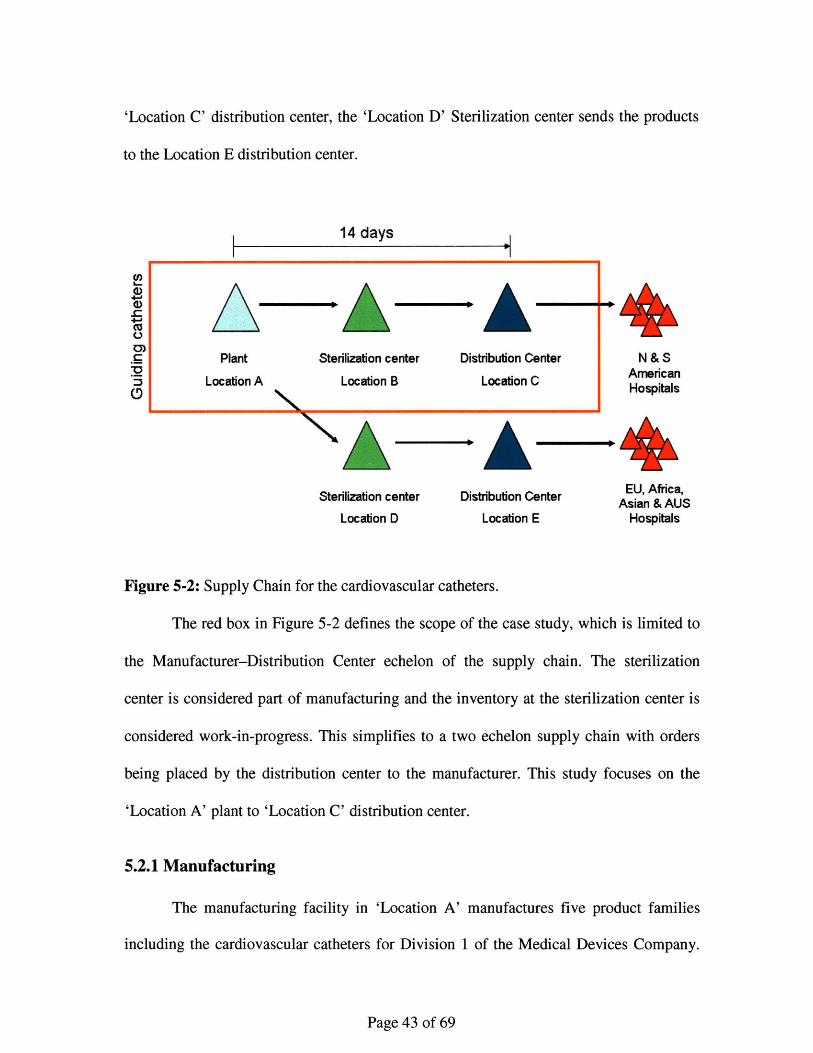
'Location C' distribution center, the 'Location D' Sterilization center sends the products

to the Location E distribution center.

14 days

Plant Sterilization center Distribution Center

Location A Location B Location C

NA ___

Sterilization center

Location D

Distribution Center

Location E

N&SAmericanHospitals

EU, Africa,Asian & AUS

Hospitals

Figure 5-2: Supply Chain for the cardiovascular catheters.

The red box in Figure 5-2 defines the scope of the case study, which is limited to

the Manufacturer-Distribution Center echelon of the supply chain. The sterilization

center is considered part of manufacturing and the inventory at the sterilization center is

considered work-in-progress. This simplifies to a two echelon supply chain with orders

being placed by the distribution center to the manufacturer. This study focuses on the

'Location A' plant to 'Location C' distribution center.

5.2.1 Manufacturing

The manufacturing facility in 'Location A' manufactures five product families

including the cardiovascular catheters for Division 1 of the Medical Devices Company.

of 69

ca.40

All the 397 SKUs of the cardiovascular catheter family are manufactured in this company

owned facility having multiple production lines. The production lines are segregated on

basis of equipment for producing a particular mix of SKUs. Some production lines are

similar and interchangeable. The average weekly demand of SKUs on these lines is 81

units and consists of a mix of all categories of SKUs. They manufacture a product mix of

358 SKUs. A particular single line manufactures a product mix of 39 SKUs. This line

manufactures low volume SKUs and the average weekly demand of SKUs produced is 30

units. The production plan is based on the inventory levels at the Location B distribution

center which transmits demand and inventory balance information to the manufacturing

plant. Based on this information, lot-sizing of the various SKUs is decided for the

manufacturing process.

5.2.2 Transportation

Transportation of product is done by trucks for intra-continental requirements and

by air for inter-continental requirements. The transportation times within the

manufacturer-sterilization plant-distribution center echelon of the supply chain are:

Transportation from Plant Location A to Location B Location A to Location Dto Sterilization Center

Transportation Time 1 day 7 daysTransportation mode Truck Airplane

Transportation from Location B to Location C Location D to Location ESterilization Center toDistribution CenterTransportation Time 2-3 days <1 dayTransportation mode Truck Truck

Table 5-1: Transportation times in the manufacturer-distribution center echelon ofcardiovascular catheter supply chain

of 69

The transportation time for the 'Location C' distribution center from the manufacturing

plant is 3-4 days, whereas the transportation time for the 'Location E' distribution center

is between 7-8 days. The former uses only truck, whereas the latter uses both trucks and

air.

The transportation time from 'Location A' plant to the 'Location B' distribution

center, which serves demand of North and South America, accounts for 21% of the total

lead time of 14 days. This case study considers the transportation time as deterministic

and does not focus upon the possibility of reduction in transportation or lead times.

5.2.3 Inventory Replenishment at Distribution Center:

The inventory and replenishment policy is defined at the SKU level. The demand

for a SKU, in terms of orders from hospitals, is received daily by the distribution center.

The demand is met by the inventory available at the distribution center. The inventory

balance is reviewed on a periodic basis by information sharing between the 'Location A'

manufacturing plant and the 'Location C' distribution center. If no stock is available at

the distribution center to meet the demand on a particular day, a back-order is generated,

and information is transmitted to the plant during the following periodic review. The

inventory replenishment is done using an (R,S) policy with a three day review period for

critical SKUs and five day review period for other SKUs. The 'criticality' of the SKU is

decided by the Medical Devices Company management depending upon various

considerations. For simplicity, this case study assumes a three day review period for all

SKUs.

The (R,S) policy has been modified by the Medical Devices Company

of 69

management due to the constraints of destructive testing to be performed on each lot of

SKUs manufactured, and taking into account cost, consolidation and batching constraints.

As a result of these considerations, whenever the inventory level at distribution center

goes below the order-up to level, a minimum order quantity is placed on the plant for

manufacture. In case, the order quantity is not sufficient to make the inventory reach the

order-up to level, a quantity equal to a multiple(s) of a constant quantity is added to the

order quantity, so that the inventory reaches at least the order-up to level. Due to these

considerations, the order-up to level does not remain fixed, but has variability around it.

Due to the considerations, the inventory level overshoots the order-up to level resulting in

an amplification of order quantity, which increases the inventory levels.

In order to assess the impact of SPC approach on bullwhip effect as compared to

the (R,S) policy, in this case study, the researchers have removed this additional

amplification of order quantity by not considering the minimum order and multiplier

constraints. The order up-to level has been considered fixed for each SKU and has been

computed on basis of the demand history.

The lead time for fulfilling the demand placed by the 'Location C' distribution

center to the plant is 14 days. It is considered to be deterministic for this case study.

5.3 Demand Characteristics of Cardiovascular catheters

Hospitals in North and South America place orders on the 'Location C'

distribution center for various SKUs of the cardiovascular catheter product family. Based

on data pertaining to the period between November 2005 and October 2006, one can

estimate the annual demand for the cardiovascular catheter family to be 1,506,100 (1.5

of 69

million) units, assuming a year of 50 weeks for this study. The data shows wide variation

in the units of various SKUs supplied by the distribution center to the hospitals.

Categories of SKUs

The SKUs can be classified on the basis of volume (units) sold into very high

volume, high volume, medium volume, small volume and very small volume SKUs.

Their distribution is indicated in table 5-2.

Category of SKUs Range of average Number of Number of unitsannual demand SKUs sold annually

(units)Very Small Volume 0-1,000 223 80,876Small Volume 1,000-5,000 118 267,056Medium Volume 5,000-15,000 39 323,449High Volume 15,000-40,000 13 350,668Very High Volume 40,000-200,000 4 484,145

Total 1,506,193Table 5-2: Distribution of SKUs on the basis of volume sold

The very small volume SKUs account for 56% of the total number of SKUs,

while small volume SKUs account for 30% of the total number of SKUs. Together, these

categories account for 86% of the total number of SKUs but only 23% of total volume.

The break-up is shown in Figure 5-3.

of 69

56%

33%30%

21% 23%18%

5% 1%

Very small Small volume Medium volume High volume Very highvolume volume

Categories of SKUs

M Percentage of total SKUs U Percentage of total demand

Figure 5-3: Break-up of the cardiovascular catheter family by categories of SKU

The very large volume SKUs account for 33% of the total demand of

cardiovascular catheters, while large volume SKUs and medium volume SKUs account

for 23% and 21% of the total demand of cardiovascular catheters respectively. The break-

up of annual demand is shown in Figure 5-3.

From the above tables and charts, Pareto analysis can be done to see that the very

high volume, high volume and medium volume SKUs, though fewer in number (14% of

total number of SKUs) account for majority (77%) of demand of the cardiovascular

catheter family. The Pareto curve for the cardiovascular catheter family is shown in

Figure 5-4.

of 69

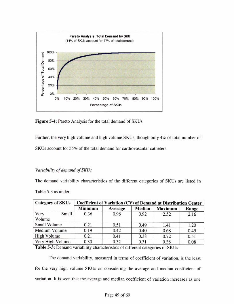
Figure 5-4: Pareto Analysis for the total demand of SKUs

Further, the very high volume and high volume SKUs, though only 4% of total number of

SKUs account for 55% of the total demand for cardiovascular catheters.

Variability of demand of SKUs

The demand variability characteristics of the different categories of SKUs are listed in

Table 5-3 as under:

Category of SKUs Coefficient of Variation (CV) of Demand at Distribution CenterMinimum Average Median Maximum Range

Very Small 0.36 0.96 0.92 2.52 2.16VolumeSmall Volume 0.21 0.51 0.49 1.41 1.20Medium Volume 0.19 0.42 0.40 0.68 0.49High Volume 0.21 0.41 0.38 0.72 0.51Very High Volume 0.30 0.32 0.31 0.38 0.08Table 5-3: Demand variability characteristics of different categories of SKUs

The demand variability, measured in terms of coefficient of variation, is the least

for the very high volume SKUs on considering the average and median coefficient of

variation. It is seen that the average and median coefficient of variation increases as one

of 69

Pareto Analysis: Total Demand by SKU(14% of SKUs account for 77% of total denand)

o 100%-

80%

W 60%0

0 40%a>

20%

0%

0% 10% 20% 30% 40% 50% 60% 70% 80% 90% 100%

Percentage of SKUs

moves from very high volume to the very small volume SKUs. The maximum coefficient

of variation increases from 0.38 to 2.52 and the range of coefficient of variation increases

from 0.08 to 2.16 as one moves from very high volume category to very small category.

The very small volume SKUs, which are 223 in number and comprise 56% of the total

SKUs, exhibit a very high variability. However, these SKUs constitute only a 5% of total

volumes of cardiovascular catheters sold.

Demand pattern at distribution center within a week

The demand pattern for the very large volume SKUs shows a wide variation

within the week. It is seen that most of the demand, in form of orders from hospitals, for

these SKUs are placed on the distribution center on Mondays (around 65%) followed by

Tuesdays (around 15%). The remaining 20% orders come on the rest of the days of the

week. The demand pattern for the distribution center can be seen from the figure 5-5. It is

evident from the figure that a large number of hospitals have a system of placing orders

during the earlier part of the week, most frequently on Mondays.

Demand Pattern for Very Large Volume SKUs

100%-

E 80%

5 60%-

a 40%-

20%

Mon Tue Wed Thu Fri

Day of Week

Figure 5-5: Demand pattern for very large volume SKUs

The effect of variation in daily ordering pattern for the very large volume SKU

of 69

category has been by mitigated by aggregating the demand at weekly level for the study.

5.4 Bullwhip Effect in the cardiovascular catheter supply chain

The present level of bullwhip on overall basis, for the cardiovascular catheter

family using a simple average is 1.17. However, given the wide variation in the demand

of the individual SKUs, it is considered more appropriate to use the weighted average,

using volume sold as the basis for measuring overall bullwhip effect. The level of

bullwhip for the cardiovascular catheter family, using the weighted average, is 1.44.

The level of bullwhip in the various categories of SKUs is listed in figure 5-6.

0.

Z'

5

4

3

2

0 --

Very SmallVolume

--

Small Volume Medium Volume High Volume

Categories of SKUs

Very HighVolume

1 fMinimum 0 Average I Median U Maximum

Figure 5-6: Level of Bullwhip in various categories of SKUs

The table indicates that, on an average, the present (R, S) policy results in

bullwhip or amplification of demand variability amongst all SKU categories except the

very small volume SKUs. All the very high volume SKUs have a significant level of

bullwhip, the level ranging from 1.40 to 1.87. All the other categories have some SKUs

of 69

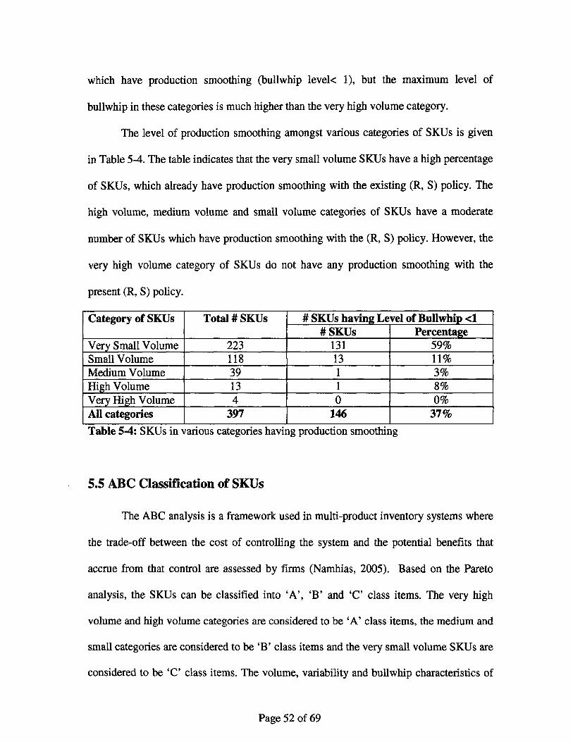
which have production smoothing (bullwhip level< 1), but the maximum level of

bullwhip in these categories is much higher than the very high volume category.

The level of production smoothing amongst various categories of SKUs is given

in Table 5-4. The table indicates that the very small volume SKUs have a high percentage

of SKUs, which already have production smoothing with the existing (R, S) policy. The

high volume, medium volume and small volume categories of SKUs have a moderate

number of SKUs which have production smoothing with the (R, S) policy. However, the

very high volume category of SKUs do not have any production smoothing with the

present (R, S) policy.

Category of SKUs Total # SKUs # SKUs having Level of Bullwhip <1# SKUs Percentage

Very Small Volume 223 131 59%Small Volume 118 13 11%Medium Volume 39 1 3%High Volume 13 1 8%Very High Volume 4 0 0%All categories 397 146 37%

Table 5-4: SKUs in various categories having production smoothing

5.5 ABC Classification of SKUs

The ABC analysis is a framework used in multi-product inventory systems where

the trade-off between the cost of controlling the system and the potential benefits that

accrue from that control are assessed by firms (Namhias, 2005). Based on the Pareto

analysis, the SKUs can be classified into 'A', 'B' and 'C' class items. The very high

volume and high volume categories are considered to be 'A' class items, the medium and

small categories are considered to be 'B' class items and the very small volume SKUs are

considered to be 'C' class items. The volume, variability and bullwhip characteristics of

of 69

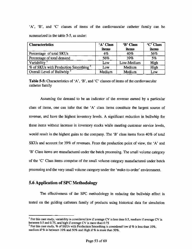
'A', 'B', and 'C' classes of items of the cardiovascular catheter family can be

summarized in the table 5-5, as under:

Characteristics 'A' Class 'B' Class 'C' Classitems items items

Percentage of total SKUs 4% 40% 56%Percentage of total demand 56% 39% 5%Variability I Low Low-Medium High% of SKUs with Production Smoothing 2 Low Medium HighOverall Level of Bullwhip : Medium Medium Low

Table 5-5: Characteristics of 'A', 'B', and 'C' classes of items of the cardiovascularcatheter family

Assuming the demand to be an indicator of the revenue earned by a particular

class of items, one can infer that the 'A' class items constitute the largest source of

revenue, and have the highest inventory levels. A significant reduction in bullwhip for

these items without increase in inventory stocks while meeting customer service levels,

would result in the highest gains to the company. The 'B' class items form 40% of total

SKUs and account for 39% of revenues. From the production point of view, the 'A' and

'B' Class items are manufactured under the batch processing. The small volume category

of the 'C' Class items comprise of the small volume category manufactured under batch

processing and the very small volume category under the 'make-to-order' environment.

5.6 Application of SPC Methodology

The effectiveness of the SPC methodology in reducing the bullwhip effect is

tested on the guiding catheters family of products using historical data for simulation

1For this case study, variability is considered low if average CV is less than 0.5, medium if average CV isbetween 0.5 and 0.75, and high if average CV is more than 0.752 For this case study, % of SKUs with Production Smoothing is considered low if % is less than 10%,medium if % is between 10% and 50% and High if % is more than 50%.

of 69

purposes. The most recent 22 weeks of historical sales is treated as future demand

information for the simulation. Six weeks of historical sales prior to this is treated as

history for the simulation and used to calibrate the demand control charts. The results of

the methodology are compared with those of a simple (R, S) policy for the same sales

data for the following metrics:

1. Coefficient of variation of order quantities

2. Average inventory

3. Fill rate

The application of the SPC methodology is demonstrated for SKU 123. The

characteristics of SKU 123 are presented below.

Average demand (historical), Y = 3,522

Standard deviation of demand (historical), Y = 1,081

Beginning on-hand inventory = 15,776

Customer service level = 99%

Lead time = 14 days

Review period = 3 days

The characteristics above are calibrated at a weekly level. The average demand is

determined by calculating the average weekly demand for each week over the 6 weeks of

history. The average of the average weekly demand is termed the average demand

(historical) in the table above. The standard deviation of demand (historical) is computed

in a similar manner. The weekly standard deviations over the 6 weeks of history are

averaged to obtain 1,081 units. For the purposes of simulation, the beginning on hand

3 For this case study, overall level of Bullwhip is considered low if average Bullwhip is less than 1.25,medium if Bullwhip is between 1.25 and 1.75 and high if bullwhip is more than 1.75

of 69

inventory for the first day of the simulation run is set as the order up to level of the (R, S)

policy. The order up to level is calculated using the formula, S=XR+L+kR+L = 15,776.

A moving window of 6 weeks of most recent history is consistently used

throughout the simulation. The set of outlier rules for this simulation are listed below.

Rule 1: If a single observation exists above +3 a limits

Rule 2: If two consecutive observations exist above the +2 a limits

Rule 3: If three consecutive observations exist above the +1 a limits

Rule 4: If six consecutive observations exist above the center line

These rules are identical to the observations below the center line with respect to the

lower control limits. These rules apply to the X chart and a chart. When any of the outlier

rules are triggered, in either of these charts, the most recent 4 weeks of observations is

averaged to determine the new location for the center line for the specific chart.

Constructing the a chart for the demand process

The values of B3 and B4 are obtained from Appendix A for a sample size of twelve.

Center line = standard deviation of demand (historical), T = 1,081

Lower control limit (LCL) = B3 Y= 383 [B 3 = 0.080 from Appendix A]

Upper control limit (UCL) = B4 s = 2,129 [B 4 = 1.970 from Appendix A]

Constructing the X chart for the demand process

The center line of the a chart represents the standard deviation of the X chart.

Center line = Average demand (historical), X = 3,522

Lower control limit (LCL) = Y - 3. = 280

of 69

Upper control limit (UCL) = X + 3. T = 6765

Monitoring the demand control charts

Every week the average of the weekly sales and standard deviation of the most

recent 6 weeks are computed. The averaged weekly standard deviation of demand is first

plotted on the Y chart and checked for outlier rules. If outlier observations exist, the

center line and control limits of the chart are updated. The control limits around the

Xchart is also updated in such a case. The twelve week averaged weekly demand is now

plotted on the X chart and tested for the outlier rules. If the outlier observations exist, the

center line of the X chart is updated. The X chart and a chart for SKU 123 over a 22-

week simulation run are shown in Figures 5-7 and 5-8.

a chart4500

40004) 3500-

30002500-

E

~1000

00 5 10 15 20

Weeks

Figure 5-7: Y chart for SKU 123

of 69

Figure 5-8: X chart for SKU 123

It can be observed from Figure 1 that at weeks 4, 10 and 19 the T chart displays

changes in the standard deviation. This results in updates in the control limits of the

Xchart. The center line of the Xchart changes once in week 7. Where the standard

deviation (from the a chart) changes, the safety stock requirement changes and where the

mean demand (from the X chart) changes, the cycle inventory changes. This is shown in

the inventory control chart (Figure 5-9).

14000

12000 -

10000 1

8000- - - - UCL

6000- - - -- LCL* * ** * "a Inventory,4000

'-ml a a 02000

00 20 40 60 80 100 120

Figure 5-9: Inventory chart for SKU 123

of 69

X-bar chart12000 ----- --- -----

10000-

8000 - -

S6000 0.- f

4000

0-~!2000

-2000 5 10 15 20

Weeks

The upper and lower control limits represents one standard deviation (-R+L)

distance from the center line. An adjustment order is not recommended by the inventory

control chart even though the inventory on two occasions drops below the lower control

limit. This is because the events do not occur on a review period. The order quantities

generated by the SPC methodology is plotted alongside that generated by the (R, S)

methodology (Figure 5-10). The coefficient of variation of the order quantities generated

by the SPC methodology is 16% compared to 42% for the (R, S) methodology suggesting

an improvement in production level loading. Additionally, the average inventory also

decreases by 7% using the SPC methodology.

(5

a

SPC vs (R, S) - Order quantity6000

5000

4000

3000

2000

1000

0

3000 .sPC

* (R, S)

1 3 5 7 9 11 13 15 17 19 21 23 25 27 29 31 33 35 37

Order period

Figure 5-10: Comparisonpolicy

of order quantities generated by SPC methodology to (R, S)

5.7 Results

The SPC based inventory management system leads to the significant reduction in

the level of bullwhip. On an overall basis for the cardio-vascular product family, the level

of 69

of bullwhip reduced by 32% from 1.17 to 0.85. By using weighted averages on the basis

of demand, the level of bullwhip reduces by 61% from 1.44 to 0.56. The SPC based

inventory management system results in production smoothing since level of bullwhip is

less than 1. Along with the reduction in bullwhip, the SPC system also results in overall

inventory reduction of 12.4%. The results obtained for the 'A', 'B' and 'C' class items

are detailed as under.

'A' Class items

The SPC based inventory management technique leads to a significant reduction

in level of bullwhip for all the seventeen 'A' class SKUs, as given in the table 5-6.

Minimum Average reduction Median reduction Maximumreduction in in Bullwhip in Bullwhip reduction in

Bullwhip Bullwhip46.8% 74.5% 76.8% 98.9%

Table 5-6: Reduction in levels of Bullwhip for 'A' class items with SPC based inventorysystem compared to the present (R,S) inventory system

This reduction in bullwhip effect was accompanied by reduction in average inventory

levels for all the SKUs, as given in table 5-7.

Minimum Average reduction Median reduction Maximumreduction in in average in average reduction in

average inventory inventory levels inventory levels average inventorylevels levels0.4% 11.8% 10.7% 33.2%

Table 5-7: Reduction in average inventory levels for 'A' class items with SPC basedinventory system compared to the present (R,S) inventory system

All of the seventeen 'A' class SKUs had 100% customer service level under the

present inventory management system, which is more than the target customer service

level of 99%. With the SPC based inventory system, all SKUs meet the 99% target

of 69

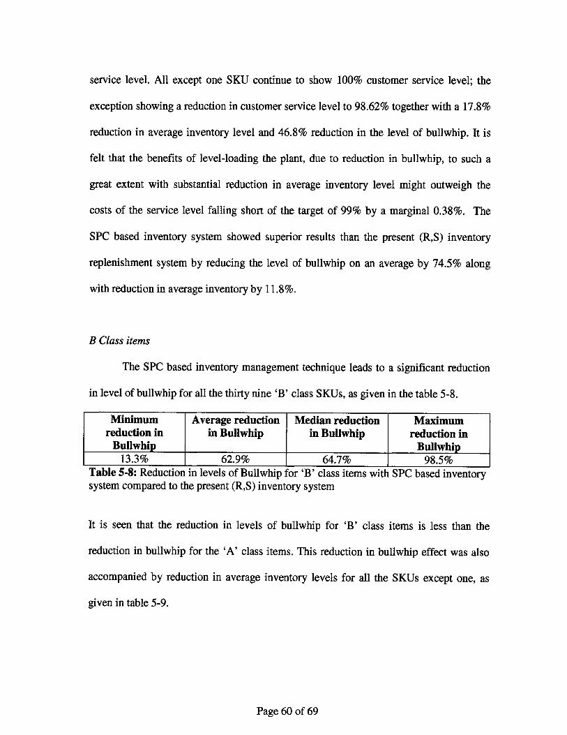
service level. All except one SKU continue to show 100% customer service level; the

exception showing a reduction in customer service level to 98.62% together with a 17.8%

reduction in average inventory level and 46.8% reduction in the level of bullwhip. It is

felt that the benefits of level-loading the plant, due to reduction in bullwhip, to such a

great extent with substantial reduction in average inventory level might outweigh the

costs of the service level falling short of the target of 99% by a marginal 0.38%. The

SPC based inventory system showed superior results than the present (R,S) inventory

replenishment system by reducing the level of bullwhip on an average by 74.5% along

with reduction in average inventory by 11.8%.

B Class items

The SPC based inventory management technique leads to a significant reduction

in level of bullwhip for all the thirty nine 'B' class SKUs, as given in the table 5-8.

Minimum Average reduction Median reduction Maximumreduction in in Bullwhip in Bullwhip reduction in

Bullwhip Bullwhip13.3% 62.9% 64.7% 98.5%

Table 5-8: Reduction in levels of Bullwhip for 'B' class items with SPC based inventorysystem compared to the present (R,S) inventory system

It is seen that the reduction in levels of bullwhip for 'B' class items is less than the

reduction in bullwhip for the 'A' class items. This reduction in bullwhip effect was also

accompanied by reduction in average inventory levels for all the SKUs except one, as

given in table 5-9.

of 69

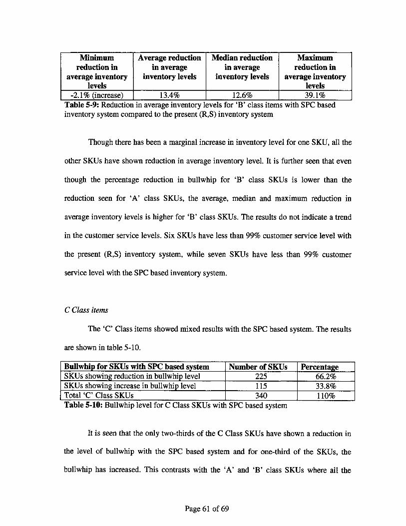
Minimum Average reduction Median reduction Maximumreduction in in average in average reduction in

average inventory inventory levels inventory levels average inventorylevels levels

-2.1% (increase) 13.4% 12.6% 39.1%Table 5-9: Reduction in average inventory levels for 'B' class items with SPC basedinventory system compared to the present (R,S) inventory system

Though there has been a marginal increase in inventory level for one SKU, all the

other SKUs have shown reduction in average inventory level. It is further seen that even

though the percentage reduction in bullwhip for 'B' class SKUs is lower than the

reduction seen for 'A' class SKUs, the average, median and maximum reduction in

average inventory levels is higher for 'B' class SKUs. The results do not indicate a trend

in the customer service levels. Six SKUs have less than 99% customer service level with

the present (R,S) inventory system, while seven SKUs have less than 99% customer

service level with the SPC based inventory system.

C Class items

The 'C' Class items showed mixed results with the SPC based system. The results

are shown in table 5-10.

Bullwhip for SKUs with SPC based system Number of SKUs PercentageSKUs showing reduction in bullwhip level 225 66.2%SKUs showing increase in bullwhip level 115 33.8%Total 'C' Class SKUs 340 110%Table 5-10: Bullwhip level for C Class SKUs with SPC based system

It is seen that the only two-thirds of the C Class SKUs have shown a reduction in

the level of bullwhip with the SPC based system and for one-third of the SKUs, the

bullwhip has increased. This contrasts with the 'A' and 'B' class SKUs where all the

of 69

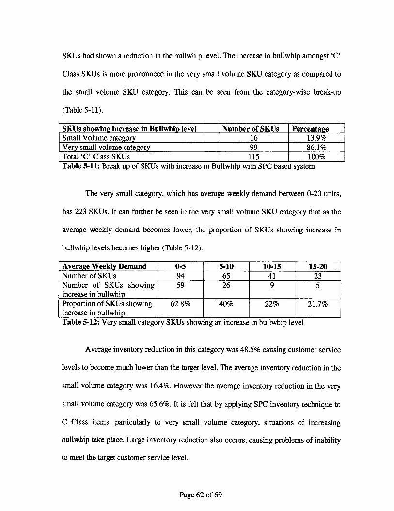
SKUs had shown a reduction in the bullwhip level. The increase in bullwhip amongst 'C'

Class SKUs is more pronounced in the very small volume SKU category as compared to

the small volume SKU category. This can be seen from the category-wise break-up

(Table 5-11).

SKUs showing increase in Bullwhip level Number of SKUs PercentageSmall Volume category 16 13.9%Very small volume category 99 86.1%Total 'C' Class SKUs 115 100%Table 5-11: Break up of SKUs with increase in Bullwhip with SPC based system

The very small category, which has average weekly demand between 0-20 units,

has 223 SKUs. It can further be seen in the very small volume SKU category that as the

average weekly demand becomes lower, the proportion of SKUs showing increase in

bullwhip levels becomes higher (Table 5-12).

Average Weekly Demand 0-5 5-10 10-15 15-20Number of SKUs 94 65 41 23Number of SKUs showing 59 26 9 5increase in bullwhipProportion of SKUs showing 62.8% 40% 22% 21.7%increase in bullwhip ITable 5-12: Very small category SKUs showing an increase in bullwhip level

Average inventory reduction in this category was 48.5% causing customer service

levels to become much lower than the target level. The average inventory reduction in the

small volume category was 16.4%. However the average inventory reduction in the very

small volume category was 65.6%. It is felt that by applying SPC inventory technique to

C Class items, particularly to very small volume category, situations of increasing

bullwhip take place. Large inventory reduction also occurs, causing problems of inability

to meet the target customer service level.

of 69

The SPC based inventory management system reduces bullwhip for the product

family by 61% using averages weighted by demand. This is accompanied by 12.4%

reduction in inventory for the family. There is significant reduction in bullwhip for 'A'

and 'B' class items with associated inventory savings while maintaining service levels.

However, for 'C' class items, customer service issues arise. Those 'C' class items having

very low demand (0 to 20 units per week) show an increase in bullwhip in addition to fill

rates issues.

of 69

6. CONCLUSIONS

Statistical Process Control is a powerful technique that can be applied to enhance

existing inventory management policies to attenuate the bullwhip effect while reducing

inventory investments and maintaining customer service levels. Specifically, the

methodology has been employed in conjunction with a simple periodic review inventory

policy - (R, S) policy. The SPC concepts can be easily adapted to benchmark and

monitor demand and inventory processes and provide a visual representation of these

processes. The methodology developed in this thesis can be configured to manage

inventory for products with a variety of demand characteristics.

The SPC methodology lends itself particularly well to Class A and B products

that have reasonably stable demand and where production level loading can provide

significant cost savings. For Class C products with sporadic demand characteristics, the

authors recommend a make-to-order policy. In such a scenario, Class C products will not

offer any practical benefits to production level loading. However, if there are a

significant number of Class C products to disrupt production efficiencies, these products

can be bundled into a single virtual product. The order quantity for the virtual product can

be planned using the SPC methodology to ensure production level loading. The order

quantities can then be allocated to actual products by ratio of their respective demand.

Special orders often arise in ordering systems which can affect the demand

characteristics of a product. For Class C products, special orders may appear more

frequently. These orders make the demand for these products very difficult to forecast.

Applying the SPC methodology to managing inventory for such products will result in a

of 69

very nervous stocking policy, potentially causing fill rate issues. This can be observed in

the case study involving the Medical Devices Company. Fulfillment of special orders

must to be managed separately and not mixed with cycle stock planning. This insulates

the demand control charts from reacting to assignable causes of demand variability that

are known in advance.

SPC determines changes in demand characteristics with a time lag resulting in

short term deficit or excess in inventory. The impact of the lag in responding to

significant changes in demand characteristics due to known events such as the addition or

loss of a customer can have tremendous immediate inventory implications. This issue can

be mitigated by updating the existing demand control charts with the expectation of

demand stemming from the planned event. Over time, the system will adjust the demand

control charts to reflect the actual nature of the demand characteristics due to this event.

The authors recognize that the methodology developed in this thesis has been

restricted to items in the mature phase of their lifecycles with a set of predefined outlier

rules. Additional research is required to explore the sensitivity of this methodology to

changes in the outlier rules and its effectiveness in the launch and declines phases of the

product lifecycle. To overcome the limitations of the methodology in addressing 'C' class

items, the demand for these items can be aggregated to create a virtual item that can be

accommodated by the methodology. However, this strategy has not been tested. Further,

since the methodology has been applied only to medical devices, the extension of this

methodology into products in other industries needs to be investigated.

of 69

BIBLIOGRAPHY

1. Beck, J. (1999). Statistical process control and selectable forecast calendars reduce

GE Aircraft Engines' parts inventory. Production and Inventory Management Journal

,40 (3), 5.

2. Boute, R. N., Disney, S. M., Lambrecht, M. R., & Houdt, B. V. (2007). An integrated

production and inventory model to dampen upstream demand variability in the supply

chain. European Journal of Operational Research, 178 (1).

3. Cardiac Catheterization. (2007). Retrieved March 2007, from American Heart

Association: http://www.americanheart.org/presenter.jhtml?identifier=4491

4. Chen, F., Drezner, Z., Ryan, J. K., & Simchi-Levi, D. (2000). Quantifying the

bullwhip effect in a simple supply chain: The impact of forecasting, lead times, and

information. Management Science, 46 (3), 8.

5. Croson, R., & Donohue, K. (2006). Behavioral causes of the bullwhip effect and the

observed value of inventory information. Management Science, 52 (3), 14.

6. Dejonckheere, J., Disney, S. M., Lambrecht, M. R., & Towill, D. R. (2004). The

impact of information enrichment on the bullwhip effect in supply chains: a control

engineering perspective. European Journal of Operational Research, 153 (4), 23.

7. Dhahri, I., & Chabchoub, H. (2007). Nonlinear goal programming models quantifying

the bullwhip effect in supply chain based on ARIMA parameters. European Journal

of Operational Research, 177 (3).

8. Disney, S. M., & Towill, D. R. (2003). The effect of vendor managed inventory

(VMI) dynamics on the bullwhip effect in supply chains. International Journal of

Production Economics, 85 (2), 16.

of 69

9. Disney, S. M., Towill, D. R., & Velde, W. v. (2004). Variance amplification and the

golden ration in production and inventory control. International Journal of

Production Economics, 90 (3).

10. Gupta, S. C. (1992). Fundamentals of statistics (5th ed.). Mumbai: Himalaya

Publishing House.

11. Hopp, W., & Spearman, M. (2000). Factory physics (2nd ed.). McGraw-Hill.

12. Huang, G. Q., Lau, J. S., & Mak, K. L. (2002). Web-based simulation portal for

investigating impacts of sharing production information on supply chain dynamics

from the perspective of inventory allocation. Integrated Manufacturing Systems , 13

(5), 14.

13. James, C. (2006, January). Manufacturing's prescription for improving health care

quality. Health Care Strategic Management, 24 (1), p. 1.

14. Jiang, W., Au, T., & Tsui, K.-L. (2007). A statistical process control approach to

business activity monitoring. IE Transactions, 39 (3), 15.

15. Lee, H. L., Padmanabhan, V., & Whang, S. (1997). Information distortion in a supply

chain: the bullwhip effect. Management Science , 43 (4), 13.

16. Lee, H. L., Padmanabhan, V., & Whang, S. (1997). The bullwhip effect in supply

chains. Sloan Management Review, 38 (3).

17. Lee, H. T., & Wu, J. C. (2006). A study on inventory replenishment policies in a two-

echelon supply chain system. Computers and Industrial Engineering, 51 (2).

18. Metters, R. (1997). Quantifying the bullwhip effect in supply chains. Journal of

Operations Management, 15 (2), 12.

19. Namhias, S. (2005). Production and operations analysis (5th ed.). McGraw-Hill.

of 69

20. Pfohl, H.-C., Cullmann, 0., & Stolzle, W. (1999). Inventory management with

statistical process control: simulation and evaluation. Journal of Business Logistics ,

20 (1), 20.

21. Prins, J. (2003, June). Shewhart X-bar and R and S Control Charts. Retrieved March

2007, from NIST/SEMATECH e-Handbook of Statistical Methods:

http://www.itl.nist.gov/div898/handbook/pmc/section3/pmc32 1.htm

22. Silver, E. A., Pyke, D. F., & Peterson, R. (1998). Inventory Management and

Production Planning and Scheduling (3rd ed.). Wiley.

23. Wong, C. Y., El-Beheiry, M. M., Johansen, J., & Hvolby, H.-H. (2007). The

implications of information sharing on bullwhip effects in a toy supply chain.

Internation Journal of Risk Assessment and Management, 7 (1).

24. Xiong, G., & Helo, P. (2006). An application of cost effective fuzzy inventory

controller to counteract demand fluctuation caused by bullwhip effect. International

Journal of Production Research, 44 (24), 16.

of 69

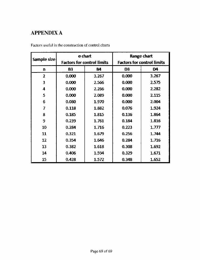
APPENDIX A

Factors useful in the construction of control charts

of 69

S o chart Range chartSample size

Factors for control limits Factors for control limits

n B3 B4 D3 D4

2 0.000 3.267 0.000 3.2673 0.000 2.566 0.000 2.5754 0.000 2.266 0.000 2.2825 0.000 2.089 0.000 2.115

6 0.080 1.970 0.000 2.004

7 0.118 1.882 0.076 1.924

8 0.185 1.815 0.136 1.864

9 0.239 1.761 0.184 1.816

10 0.284 1.716 0.223 1.777

11 0.321 1.679 0.256 1.744

12 0.354 1.646 0.284 1.716

13 0.382 1.618 0.308 1.692

14 0.406 1.594 0.329 1.671

15 0.428 1.572 0.348 1.652

Statistical Process Control Approach to Reduce the ...

Documents

Transcript of Statistical Process Control Approach to Reduce the ...