Statistical Power Analysis with Missing Data, Adam Davey andJyoti Savla
386
description
"There is very little in the field about the effect of missing data on statistical power. This is an importantarea that needs to be addressed ... The writing style is ... easy to read and engaging ... This book will ... beused as a supplement in power analysis and SEM classes ... and by ... indivlduals that are currentlycalculating power for research studies ..• this book fills an important gap in the published literature."-Jay Maddock, University of Hawaii at Manoa"This text fills an enormous hole in the literature, and is sorely needed ... the clear writing, examples,and syntax for a variety of programs are major strengths ... lt will make a major and lasting contribution tothe field ... everythlng that I would want in a text for doctoral students is here."- Jim Deal, North Dakota State University" ... a valuable contribution to researchers conducting structural equation modeling research as wellas to researchers in general in helping to inform on basic issues of missing data ... reader friendly andaccessible for all ... The quality of scholarship is high. lt is evident the authors understand the material."- Debbie Hahs-Vaughn, University of Central Florida"The book has the potential to add to the research literature .. .in terms of how to do statistical poweranalysis with missing data ... I would definitely buy this book because of the programs and Instructionsfor power calculations for covariance structure models!'- David P. MacKinnon, Arizona State UniversityStatistical power analysis has revolutionized the ways in which we conduct and evaluate research. Similardevelopments in the statistical analysis of incomplete (missing) data are gaining more widespread applications.This volume brings statistical power and incomplete data together under a common framework, in a way thatis readily accessible to those with only an introductory familiarity with structural equation modeling. lt answersmany practical questions such as:• how missing data affects the statistical power in a study• how much power is likely with different amounts and types of missing data• how to increase the power of a design in the presence of missing data, and• how to identify the most powerful design In the presence of missing data.Points of Reflection encourage readers to stop and test their understanding of the material. Try Me sectionstest one's ability to apply the material. Troubleshooting Tips help to prevent commonly encountered problems.Exercises reinforce content and Additional Readings provide sources for delving more deeply into selected topics.Numerous examples demonstrate the book's application to a variety of disciplines. Each issue is accompanied byits potential strengths and shortcomings and examples using a variety of software packages (SAS, SPSS, Stata,USREL, AMOS, and MPius). Syntax is provided using a single software program to promote continuity but in eachcase, parallel syntax using the other packages is presented in appendixes. Routines, data sets, syntax files, andlinks to student versions of software packages are found at www.psypress.com/davey. The worked examplesin Part 2 also provide results from a wider set of estimated models. These tables, and accompanying syntax, canbe used to estimate statistical power or required sample size for similar problems under a wide range of conditions.Class-tested at Temple, Virginia Tech, and Miami University of Ohio, this brief text is an ideal supplement forgraduate courses in applied statistics, statistics 11, intermediate or advanced statistics, experimental design,structural equation modeling, power analysis, and research methods taught in departments of psychology, humandevelopment, education, sociology, nursing, social work, gerontology and other social and health sciences. The book'sapplied approach wlll also appeal to researchers in these areas. Sections covering Fundamentals, Applications,and Extensions ar
Transcript of Statistical Power Analysis with Missing Data, Adam Davey andJyoti Savla

Statistical Power Analysis
with Missing Data
Y100315.indb 1 7/15/09 2:58:41 PM

Y100315.indb 2 7/15/09 2:58:41 PM
New York London
Statistical Power Analysis
with Missing DataA Structural Equation Modeling Approach
Adam DaveyTemple University
Jyoti SavlaVirginia Polytechnic Institute
and State University
Y100315.indb 3 7/15/09 2:58:41 PM

Visit the Family Studies Arena Web site at: www.family-studies-arena.com
RoutledgeTaylor & Francis Group270 Madison AvenueNew York, NY 10016
RoutledgeTaylor & Francis Group27 Church RoadHove, East Sussex BN3 2FA
© 2010 by Taylor and Francis Group, LLCRoutledge is an imprint of Taylor & Francis Group, an Informa business
Printed in the United States of America on acid-free paper10 9 8 7 6 5 4 3 2 1
International Standard Book Number: 978-0-8058-6369-7 (Hardback) 978-0-8058-6370-3 (Paperback)
For permission to photocopy or use material electronically from this work, please access www.copyright.com (http://www.copyright.com/) or contact the Copyright Clearance Center, Inc. (CCC), 222 Rosewood Drive, Danvers, MA 01923, 978-750-8400. CCC is a not-for-profit organiza-tion that provides licenses and registration for a variety of users. For organizations that have been granted a photocopy license by the CCC, a separate system of payment has been arranged.
Trademark Notice: Product or corporate names may be trademarks or registered trademarks, and are used only for identification and explanation without intent to infringe.
Library of Congress Cataloging-in-Publication Data
Davey, Adam.Statistical power analysis with missing data : a structural equation modeling
approach / Adam Davey, Jyoti Savla.p. cm.
Includes bibliographical references and index.ISBN 978-0-8058-6369-7 (hbk. : alk. paper) -- ISBN 978-0-8058-6370-3 (pbk.: alk. paper)1. Social sciences--Statistics. 2. Social sciences--Statistical methods. 3. Social
sciences--Mathematical models. I. Savla, Jyoti. II. Title.
HA29.D277 2010519.5--dc22 2009026347
Visit the Taylor & Francis Web site athttp://www.taylorandfrancis.com
and the Psychology Press Web site athttp://www.psypress.com
Y100315.indb 4 7/15/09 2:58:42 PM
Contents
1 Introduction ............................................................................................... 1Overview and Aims ................................................................................... 1Statistical Power .......................................................................................... 5
Testing Hypotheses ............................................................................... 6Choosing an Alternative Hypothesis .................................................. 7Central and Noncentral Distributions ................................................ 7Factors Important for Power ................................................................. 9Effect Sizes ............................................................................................ 10Determining an Effect Size ................................................................. 12Point Estimates and Confidence Intervals ........................................ 14Reasons to Estimate Statistical Power ............................................... 17
Conclusions ................................................................................................ 17Further Readings ...................................................................................... 18
ISection Fundamentals
2 The LISREL Model ................................................................................. 21Matrices and the LISREL Model ............................................................. 22Latent and Manifest Variables ................................................................ 24
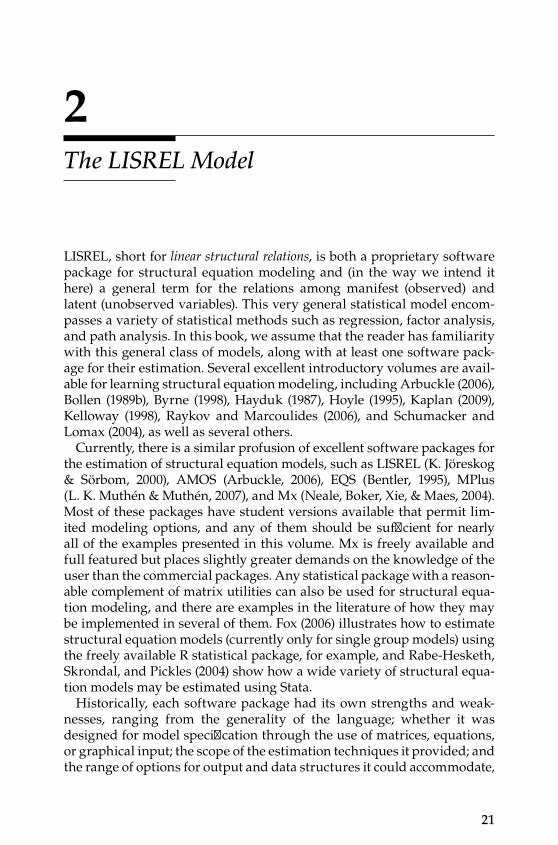
Regression Coefficient Matrices ......................................................... 25Variance‑Covariance Matrices ........................................................... 25Vectors of Means and Intercepts ........................................................ 26
Model Parameters ..................................................................................... 27Models and Matrices ........................................................................... 30Structure of a LISREL Program ......................................................... 34Reading and Interpreting LISREL Output ....................................... 38Evaluating Model Fit ........................................................................... 41Measures of Population Discrepancy ............................................... 42
Incremental Fit Indices ................................................................... 42Absolute Fit Indices ......................................................................... 43
Conclusions ................................................................................................ 43Further Readings ...................................................................................... 43
3 Missing Data: An Overview ................................................................. 47Why Worry About Missing Data? .......................................................... 47Types of Missing Data .............................................................................. 48
Y100315.indb 5 7/15/09 2:58:42 PM
vi Contents
Missing Completely at Random ......................................................... 48Missing at Random .............................................................................. 49Missing Not at Random ...................................................................... 49
Strategies for Dealing With Missing Data ............................................. 51Complete Case Methods ..................................................................... 51List‑Wise Deletion ................................................................................ 51List‑Wise Deletion With Weighting ................................................... 51Available Case Methods ...................................................................... 52Pair‑Wise Deletion ............................................................................... 52Expectation Maximization Algorithm .............................................. 52Full Information Maximum Likelihood ........................................... 53
Imputation Methods ................................................................................. 54Single Imputation ................................................................................. 54Multiple Imputation ............................................................................. 55
Estimating Structural Equation Models With Incomplete Data ........ 56Conclusions ................................................................................................ 64Further Readings ...................................................................................... 65
4 Estimating Statistical Power With Complete Data .......................... 67Statistical Power in Structural Equation Modeling ............................. 67Power for Testing a Single Alternative Hypothesis ............................. 68
Tests of Exact, Close, and Not Close Fit ............................................ 72Tests of Exact, Close, and Not Close Fit Between Two Models ..... 75
An Alternative Approach to Estimate Statistical Power ..................... 76Estimating Required Sample Size for Given Power ............................ 78Conclusions ................................................................................................ 80Further Readings ...................................................................................... 80
ISection I Applications
5 Effects of Selection on Means, Variances, and Covariances .......... 89Defining the Population Model .............................................................. 90
Defining the Selection Process ........................................................... 92An Example of the Effects of Selection ............................................. 93
Selecting Data Into More Than Two Groups ........................................ 99Conclusions .............................................................................................. 101Further Readings .................................................................................... 102
6 Testing Covariances and Mean Differences With Missing Data .......................................................................................................... 103Step 1: Specifying the Population Model ............................................ 104Step 2: Specifying the Alternative Model ............................................ 105
Y100315.indb 6 7/15/09 2:58:42 PM
Contents vii
Step 3: Generate Data Structure Implied by the Population Model ....................................................................................................106Step 4: Decide on the Incomplete Data Model .................................... 106Step 5: Apply the Incomplete Data Model to Population Data ........ 106Step 6: Estimate Population and Alternative Models With Missing Data .................................................................................. 109Step 7: Using the Results to Estimate Power or Required Sample Size ...............................................................................................110Conclusions ...............................................................................................117Further Readings .....................................................................................117
7 Testing Group Differences in Longitudinal Change .................... 119The Application ........................................................................................119The Steps .................................................................................................. 122
Step 1: Selecting a Population Model .............................................. 123Step 2: Selecting an Alternative Model ........................................... 124Step 3: Generating Data According to the Population Model ..... 125Step 4: Selecting a Missing Data Model .......................................... 126Step 5: Applying the Missing Data Model to Population Data ... 127Step 6: Estimating Population and Alternative Models With Incomplete Data ........................................................................ 128Step 7: Using the Results to Calculate Power or Required Sample Size ......................................................................................... 136
Conclusions .............................................................................................. 140Further Readings .....................................................................................141
8 Effects of Following Up via Different Patterns When Data Are Randomly or Systematically Missing ....................................... 143Background .............................................................................................. 143The Model ................................................................................................ 145
Design .................................................................................................. 146Procedures ........................................................................................... 148Evaluating Missing Data Patterns ................................................... 152
Extensions to MAR Data ........................................................................ 158Conclusions .............................................................................................. 164Further Readings .................................................................................... 164
9 Using Monte Carlo Simulation Approaches to Study Statistical Power With Missing Data ................................................ 165Planning and Implementing a Monte Carlo Study ............................ 165Simulating Raw Data Under a Population Model .............................. 170
Generating Normally Distributed Univariate Data ...................... 171Generating Nonnormally Distributed Univariate Data ............... 172
Y100315.indb 7 7/15/09 2:58:42 PM

viii Contents
Generating Normally Distributed Multivariate Data ....................174Generating Nonnormally Distributed Multivariate Data ............ 177
Evaluating Convergence Rates for a Given Model ............................. 178Step 1: Developing a Research Question ........................................ 180Step 2: Creating a Valid Model ......................................................... 180Step 3: Selecting Experimental Conditions .................................... 180Step 4: Selecting Values of Population Parameters ....................... 181Step 5: Selecting an Appropriate Software Package ..................... 182Step 6: Conducting the Simulations ................................................ 182Step 7: File Storage .............................................................................. 182Step 8: Troubleshooting and Verification ........................................ 183Step 9: Summarizing the Results ..................................................... 184
Complex Missing Data Patterns ........................................................... 186Conclusions .............................................................................................. 190Further Readings .................................................................................... 191
IISection I Extensions
10 Additional Issues With Missing Data in Structural Equation Models ................................................................................... 207Effects of Missing Data on Model Fit ................................................... 207Using the NCP to Estimate Power for a Given Index .........................211Moderators of Loss of Statistical Power With Missing Data .............211
Reliability .............................................................................................211Auxiliary Variables ............................................................................ 215
Conclusions .............................................................................................. 218Further Readings .................................................................................... 219
11 Summary and Conclusions ................................................................. 231Wrapping Up ........................................................................................... 231Future Directions .................................................................................... 232Conclusions .............................................................................................. 233Further Readings .................................................................................... 233
References ...................................................................................................... 235
Appendices .....................................................................................................243
Index ................................................................................................................ 359
Y100315.indb 8 7/15/09 2:58:42 PM

Preface
Statistical power analysis has revolutionized the ways in which behavioral and social scientists plan, conduct, and evaluate their research. Similar developments in the statistical analysis of incomplete (missing) data are gaining more widespread applications as software catches up with theory. However, very little attention has been devoted to the ways in which miss‑ing data affect statistical power. In fields such as psychology, sociology, human development, education, gerontology, nursing, and health sciences, the effects of missing data on statistical power are significant issues with the potential to influence how studies are designed and implemented.
Several factors make these issues (and this book) significant. First and foremost, data are expensive and difficult to collect. At the same time, data collection with some groups may be taxing. This is particularly true with today’s multidisciplinary studies where researchers often want to com‑bine information across multiple (e.g., physiological, psychological, social, contextual) domains. If there are ways to economize and at the same time reduce expense and testing burden through application of missing data designs, then these should be identified and exploited in advance when‑ever possible.
Second, missing data are a nearly inevitable aspect of social science research and this is particularly true in longitudinal and multi‑informant studies. Although one might expect that any missing data would simply reduce power, recent research suggests that not all missing data were cre‑ated equal. In other words, some types of missing data may have greater implications for loss of statistical power than others. Ways to assess and anticipate the extent of loss in power with regard to the amount and type of missing data need to be more widely available, as do ways to moderate the effects of missing data on the loss of statistical power whenever possible.
Finally, some data are inherently missing. A number of “incomplete” designs have been considered for some time, including the Solomon four‑group design, Latin squares design, and Schaie’s most efficient design. However, they have not typically been analyzed as missing data designs. Planning a study with missing data may actually be a cost‑effective alter‑native to collecting complete data on all individuals. For some applications, these “missing by design” methods of data collection may be the only prac‑tical way to plan a study, such as with accelerated longitudinal designs. Knowing how best to plan a study of this type is increasingly important.
Y100315.indb 9 7/15/09 2:58:42 PM

x Preface
This volume brings statistical power and incomplete data together under a common framework. We aim to do so in a way that is readily accessible to social scientists and students who have some familiarity with struc‑tural equation modeling. Our book is divided into three sections. The first presents some necessary fundamentals and includes an introduction and overview as well as chapters addressing the topics of the LISREL model, missing data, and estimating statistical power in the complete data con‑text. Each of these chapters is designed to present all of the information necessary to work through all of the content of this book. Though a certain amount of familiarity with topics such as hypothesis testing or structural equation models (with any statistical package) is required, we have made every effort to ensure that this content is accessible to as wide a readership as possible. If you are not very familiar with structural equation model‑ing or have not spent much time working with a software package that estimates these models, we strongly encourage you to work slowly and carefully through the Fundamentals section until you feel confident in your abilities. All of the subsequent materials covered in this book draw directly on the material covered in this first section. Even if you are very comfortable with your structural equation modeling skills, we still recom‑mend that you review this material so that you will be familiar with the conventions we use in the remainder of this volume.
The second section of this book presents several applications. We con‑sider a wide variety of fully worked examples, each building one step at a time beyond the preceding application or considering a different approach to an issue that has been considered earlier. In Chapter 5, we begin by con‑sidering the effects of selection on means, variances, and covariances as a way of introducing data that are missing in a systematic fashion. This is the most intensive chapter of the book, in terms of the formulas and equations we introduce, so we try to make each of the steps build directly on what has been done earlier. Next, we consider how structural equation models can be used to estimate models with incomplete data. In a third application, we extend this approach to a model of considerable substan‑tive interest, such as testing group differences in a growth curve model. Because of the realistic nature of this application, Chapter 8 is thus the most intensive chapter in terms of syntax. Again, we have made every effort to ensure that each piece builds slowly and incrementally on what has come before. Additional applications work through an example of a study with data missing by design and using a Monte Carlo approach (i.e., simulating and analyzing raw data) to estimate statistical power with incomplete data. In addition to the specific worked examples, these chap‑ters provide results from a wider set of estimated models. These tables, and accompanying syntax, can be used to estimate statistical power or required sample size for similar problems under a wide range of condi‑tions. We encourage all readers to run the accompanying syntax in the
Y100315.indb 10 7/15/09 2:58:42 PM

Preface xi
software packages of their choice in order to ensure that your results agree with the ones we present in the text. If your results do not agree with our results, then something needs to be resolved before moving for‑ward through the material. We have tried to indicate key points in the material where you should stop and test your understanding of the mate‑rial (“Points of Reflection”) or your ability to apply it to a specific problem (“Try Me”), as well as “Troubleshooting Tips” that can help to remedy or prevent commonly encountered problems. Exercises at the end of each chapter are designed to reinforce content up to that point and, in places, to foreshadow content of the subsequent chapter. Try at least a few of them before moving on to the next chapter. We also provide a list of additional readings to help readers learn more about basic issues or delve more deeply into selected topics in as efficient a manner as possible.
The third section of this book presents a number of extensions to the approaches outlined here. Material covered in this section includes dis‑cussion of a number of factors that can moderate the effects of missing data on loss of statistical power from a measurement, design, or analysis perspective and extends the discussion beyond testing of hypotheses for a specific model parameter to consider evaluation of model fit and effects of missing data on a variety of commonly used fit indices. Our conclud‑ing chapter integrates much of the content of the book and points toward some useful directions for future research.
Every social scientist knows that missing data and statistical power are inherently associated, but currently almost no information is available about the precise relationship. The proposed book fills this large gap in the applied methodology literature while at the same time answering practi‑cal and conceptual questions such as how missing data may have affected the statistical power in a specific study, how much power a researcher will have with different amounts and types of missing data, how to increase the power of a design in the presence or expectation of missing data, and how to identify the more statistically powerful design in the presence of missing data.
This volume selectively integrates material across a wide range of con‑tent areas as it has developed over the past 50 (and particularly the past 20) years, but no single volume can pretend to be complete or compre‑hensive across such a wide content area. Rather, we set out to present an approach that combines a reasonable introduction to each issue, its poten‑tial strengths and shortcomings, along with plenty of worked examples using a variety of popular software packages (SAS, SPSS, Stata, LISREL, AMOS, MPlus).
Where necessary, we provide sufficient material in the form of equa‑tions and advanced readings to appeal to individuals in search of in‑depth knowledge in this area, while serving the primary audience of individu‑als who need this kind of information in order to plan and evaluate their
Y100315.indb 11 7/15/09 2:58:42 PM

xii Preface
own research. Skip anything that does not make sense on a first reading, with our blessing — just plan to return to it again after working through the examples further. Our writing style should be accessible to all indi‑viduals with an introductory to intermediate familiarity with structural equation modeling.
We believe that nearly all students and researchers can successfully delve further into the methodological literature than they may currently be comfortable, and that Greek (i.e., the equations we have included through‑out the text) only hurts until you have applied it to a specific example. There are locations in the text where even very large and unwieldy equa‑tions reduce down to simple arithmetic that you can literally do by hand. Throughout this volume, we have tried to explain the meaning of each equation in words as well as provide syntax to help you to turn the equa‑tions into numbers with more familiar meanings. This may sound like a strange thing to say in a book about statistics, but leave as little to chance as possible. Take our word for it that you will get considerably more ben‑efit from this text if you stop and test out each example along the way than if you allow the mathematics and equations to remain abstract rather than applying them each step of the way. After all, what’s the worst thing that could happen?
We recognize that we cannot hope to please all of the people all of the time with a volume such as this one. As such, this book reflects a num‑ber of compromises as well as a number of accommodations. In the text, we present syntax using a single software program to promote continu‑ity of the material. We have strived to choose the software that provides answers most directly or that maps most closely onto the way in which the content is discussed. In each case, however, parallel syntax using the other packages is presented as an appendix to each chapter. Additionally, we include a link to Web resources with each of the routines, data sets, and syntax files referred to in the book, as well as links to additional mate‑rial, such as student versions of each software package that can be used to estimate all examples included in this book.
As of the time of writing, each of the structural equation modeling syntax files has been tested on LISREL version 8.8, MPlus version 4.21, and AMOS version 7. Syntax in other statistical packages has been imple‑mented with SPSS version 15, SAS version 9, and Stata version 10.
Finally, a great many people helped to make this book both possible and plausible. We wish to offer sincere thanks to our spouses, Maureen and Sital, for helping us to carve out the time necessary for an undertaking such as this one. We discovered that what started as a simple and straight‑forward project would have to first be fermented and then distilled, and we appreciate your patience through this process. Zupei Luo joined our efforts early and made several solid contributions to our thinking. Many students and colleagues provided input and plenty of constructive criticism along
Y100315.indb 12 7/15/09 2:58:42 PM

Preface xiii
the way. These included presentations of some of our initial ideas at Miami University (Kevin R. Bush and Rose Marie Ward, Pete Peterson, and Aimin Wang were regular contributors) and Oregon State University (Alan Acock, Karen Hooker, Alexis Walker). Several of our students and colleagues, first through projects at the University of Georgia (Shayne Anderson, Steve Beach, Gene Brody, Rex Forehand, Xiaojia Ge, Megan Janke, Mark Lipsey, Velma Murry, Bob Vandenberg, Temple University (Michelle Bovin, Hanna Carpenter, Nicole Noll), and beyond (Anne Edwards, Scott Maitland, Larry Williams), helped us figure out what we were really trying to say. We also owe a significant debt of gratitude to four reviewers (Jim Deal, David MacKinnon, Jay Maddock, and Debbie Hahs‑Vaughn) who provided us with precisely the kind of candid feedback we needed to improve the quality of this book. Thank you for both making the time and for telling us what we needed to hear. We sincerely hope that we have successfully incorporated all of your suggestions. Finally, we wish to acknowledge the steady support and encouragement of Debra Riegert, Christopher Myron, and Erin Flaherty and the many others at Taylor and Francis who helped bring this project to fruition. All remaining deficiencies in this volume rest squarely on our shoulders.
Y100315.indb 13 7/15/09 2:58:42 PM

Y100315.indb 14 7/15/09 2:58:43 PM

1
1Introduction
Overview and Aims
Missing data are a nearly ubiquitous aspect of social science research. Data can be missing for a wide variety of reasons, some of which are at least partially controllable by the researcher and others that are not. Likewise, the ways in which missing data occur can vary in their implications for reaching valid inferences. This book is devoted to helping researchers consider the role of missing data in their research and to plan appro‑priately for the implications of missing data. Recent years have seen an extremely rapid rise in the availability of methods for dealing with miss‑ing data that are becoming increasingly accessible to non‑methodologists. As a result, their application and acceptance by the research community has expanded exponentially.
It was not so very long ago that even highly sophisticated researchers would, at best, acknowledge the extent of missing data and then proceed to present analyses based only on the subset of participants who provided complete data for the variables of interest. This “list‑wise deletion” treat‑ment of missing values remains the default option in nearly every statisti‑cal package available to social scientists.
Researchers who attempted to address issues of missing data in more sophisticated ways risked opening themselves to harsh criticism from reviewers and journal editors, often being accused of making up data or being treated as though their methods were nothing more than statisti‑cal sleight of hand. In reality, it usually requires stronger assumptions to ignore missing data than to address them. For example, the assumptions required to reach valid conclusions based on list‑wise deletion actually require a much greater leap of faith than the use of more sophisticated approaches.
Fortunately, the times have changed quickly as statistical software developers have gone to greater lengths to incorporate appropriate tech‑niques in their software. At the same time, many social scientists with sophisticated methodological skills have helped to facilitate a better con‑ceptual understanding of missing data issues among non‑methodologists
Y100315.indb 1 7/15/09 2:58:43 PM

2 Statistical Power Analysis with Missing Data
(e.g., Acock, 2005; Allison, 2001; Schafer & Graham, 2002). There is now the general expectation within the scientific community that researchers will provide more sophisticated treatment of missing data. However, the implications of missing data for social science research have not received widespread treatment to date, nor have they made their way into the plan‑ning of sound research, being something to anticipate and perhaps even incorporate deliberately.
Statistical power is the probability that one will find an effect of a given magnitude if in fact one actually exists. Although statistical power has a long history in the social sciences (e.g., Cohen, 1969; Neyman & Pearson, 1928a, 1928b), many studies remain underpowered to this day (Maxwell, 2004; Maxwell, Kelly, & Rausch, 2008). Given that the success of publish‑ing one’s results and obtaining funding typically rest upon reliably iden‑tifying statistically significant associations (although there is a growing movement away from null hypothesis significance testing; see Harlow, Mulaik, & Steiger, 1997), there is considerable importance to learning how to design and conduct appropriate power analyses, in order to increase the chances that one’s research will be informative and in order to work toward building a cumulative body of knowledge (Lipsey, 1990). In addi‑tion to determining whether means differ, assumptions (e.g., normality, homoscedasticity, etc.) are met, or a more parsimonious model performs as well as one that is more complex, there is greater recognition today that statistically significant results are not always meaningful, which places increased emphasis on the choice of alternative hypotheses.
We have several aims in this volume. First, we hope to provide social scientists with the skills to conduct a power analysis that can incorpo‑rate the effects of missing data as they are expected to occur. A second aim is to help researchers move missing data considerations forward in their research process. At present, most researchers do not truly begin to consider the influence of missing data until the analysis stage (e.g., Molenberghs & Kenward, 2007). This volume can help researchers to carry the role of missing data forward to the planning stage, before any data are even collected or a grant proposal is even submitted.
Power analyses that consider missing data can provide more accurate estimates of the likelihood of success in a study. Several of the consider‑ations we address in this book also have implications for ways to reduce the potential effects of missing data on loss of statistical power, many under the researcher’s control. Finally, we hope that this volume will pro‑vide an initial framework in which issues of missing data and their asso‑ciations with statistical power can become better explored, understood, and even exploited.
As resources to conduct research become more difficult to obtain, the importance of statistical power grows as well, along with demands on researchers to plan studies as efficiently as possible. At the same time,
Y100315.indb 2 7/15/09 2:58:43 PM
Introduction 3
the increase in application of complex multivariate statistics and latent variable models afforded by greater computing power also places heavier demands on data and samples. In the context of structural equation mod‑eling, there is generally also a greater theoretical burden on researchers prior to the conduct of their analyses. It is important for researchers to know quite a bit in advance about their constructs, measures, and models. The process of hypothesis testing has become multivariate and, particu‑larly in nonexperimental contexts, subsequent stages of analysis are often predicated on the outcomes of previous stages. Fortunately, it is precisely these situations that lend themselves most directly to power analysis in the context of structural equation modeling.
History is also on our side. Designs that incorporate missing data (so‑called incomplete designs) have been a part of the social sciences for a very long time, although we do not often think of them in this way. Some of the classic examples include the Solomon four‑group design for evaluating testing by treatment interactions (Campbell & Stanley, 1963; Solomon, 1949) and the Latin squares design. More recent exam‑ples include cohort‑sequential, cross‑sequential, and accelerated longi‑tudinal designs (cf. Bell, 1953; McArdle & Hamagami, 1991; Raudenbush & Chan, 1992; Schaie, 1965). However, with the exception of the latter example, these designs have not typically been analyzed as missing data designs but rather analyzed piecewise according to complete data principles.
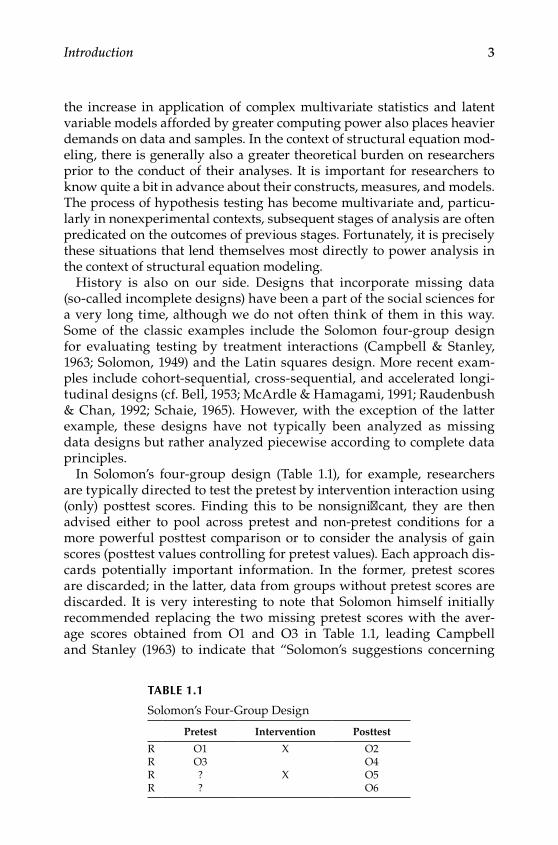
In Solomon’s four‑group design (Table 1.1), for example, researchers are typically directed to test the pretest by intervention interaction using (only) posttest scores. Finding this to be nonsignificant, they are then advised either to pool across pretest and non‑pretest conditions for a more powerful posttest comparison or to consider the analysis of gain scores (posttest values controlling for pretest values). Each approach dis‑cards potentially important information. In the former, pretest scores are discarded; in the latter, data from groups without pretest scores are discarded. It is very interesting to note that Solomon himself initially recommended replacing the two missing pretest scores with the aver‑age scores obtained from O1 and O3 in Table 1.1, leading Campbell and Stanley (1963) to indicate that “Solomon’s suggestions concerning
Table 1.1
Solomon’s Four‑Group Design
Pretest Intervention Posttest
R O1 X O2R O3 O4R ? X O5R ? O6
Y100315.indb 3 7/15/09 2:58:43 PM

4 Statistical Power Analysis with Missing Data
these are judged unacceptable” (p. 25) and to suggest that pretest scores essentially be discarded from analysis. If you think about it, the random assignment to groups in this design suggests that the mean of O1 and O3 is likely to be the best estimate, on average, of the pretest means for the groups for which pretest scores were deliberately unobserved. How modern approaches differ from Solomon’s suggestion is that they cap‑ture not just these point estimates, but they also factor in an appropriate degree of uncertainty regarding the unobserved pretest scores. In this design, randomization allows the researcher to make certain assump‑tions about the data that are deliberately not observed.
In contrast, compare this approach with the accelerated longitudinal design, illustrated in Table 1.2. Here, one can deliberately sample three (or more) different cohorts on three (or more) different occasions and subse‑quently reconstruct a trajectory of development over a substantially lon‑ger period of development by simultaneously analyzing data from these incomplete trajectories. In this minimal example, just 2 years (with three waves of data collection) of longitudinal research yields information about 4 years of development with, of course, longer periods possible through the addition of more waves and cohorts. Different assumptions, such as the absence of cohort differences, are required in order for this design to be valid. However, careful design can also allow for appropriate evalu‑ation of these assumptions and remediation in cases where they are not met. In fact, testing of some hypotheses would not even be possible using a complete data design, as is the case with Solomon’s four‑group design.
On the other hand, an incomplete design means that it may not be pos‑sible to estimate all parameters of a model. Because it is never observed, the correlation between variables at ages 12 and 16 cannot be estimated in the example above. Often, however, this has little bearing on the questions we wish to address, or else we can design the study in a way that allows us to capture the desired information.
This book has been designed with several goals in mind. First and fore‑most, we hope that it will help researchers and students from a variety of disciplines, including psychology, sociology, education, communication,
Table 1.2
Accelerated Longitudinal Design
Age
12 13 14 15 16
Cohort 1 O O O ? ?
Cohort 2 ? O O O ?Cohort 3 ? ? O O O
Y100315.indb 4 7/15/09 2:58:43 PM

Introduction 5
management, nursing, and social work, to plan better, more informative studies by considering the effects that missing data are likely to have on their ability to reach valid and replicable inferences.
It seems rather obvious that whenever we are missing data, we are miss‑ing information about the population parameters for which we wish to reach inferences, but learning more about the extent to which this is true and, more importantly, steps that researchers can take to reduce these effects, forms another important objective of this book. As we will see, all missing data were not created equal, and it is very often possible to con‑duct a more effective study by purposefully incorporating missing data into its design (e.g., Graham, Hofer, & MacKinnon, 1996).
Even the statistical literature has devoted considerably more attention to ways in which researchers can improve statistical power over and above list‑wise deletion methods, rather than to consider how appropri‑ate application of these techniques compares with availability of com‑plete data. Under at least some circumstances, researchers may be able to achieve greater statistical power by incorporating missing data into their designs.
A third goal of this volume is to help researchers to anticipate and eval‑uate contingencies before committing to a specific course of action and to be in a better position to evaluate one’s findings. In this sense, conducting rigorous power analyses appropriate to the range of missing data situa‑tions and statistical analyses faced in a typical study is analogous to the role played by pilot research when one is developing measures, manipula‑tions, and designs appropriate to testing hypotheses. As we shall see, the techniques presented in this book are appropriate to both experimental and nonexperimental contexts and to situations where data are missing either by default or by design. They can be used as well, with only minor modifications, in either an a priori or a posteriori fashion and with a single parameter of interest or in order to evaluate an entire model just as in the complete data case (e.g., Hancock, 2006; Kaplan, 1995).
Statistical Power
Because the practical aspects of statistical power do not always receive a great deal of attention in many statistics and research methods courses, before launching into consideration of statistical power, we begin by first reviewing some of the components and underlying logic associated with statistical power. The rest of this book elaborates on the importance of each of these elements in the examples presented.
Y100315.indb 5 7/15/09 2:58:43 PM

6 Statistical Power Analysis with Missing Data
Testing Hypotheses
One of the purposes of statistical inference is to test hypotheses about the (unknown) state of affairs in the world. How many people live in pov‑erty? Do boys and girls differ in mathematical problem‑solving ability? Does smoking cause cancer? Will seat belts reduce the number of fatali‑ties in automobile accidents? Is one drug more effective in reducing the symptoms of a specific disease than another? Our goal in these situations is almost always to reach valid inferences about a population of interest and to address our question. Setting aside for a moment that outcomes almost always result from multiple causes and that our measurement of both predictors and outcomes is typically fraught with at least some error or unreliability, it is almost never possible (or necessary or even advisable) to survey all members of that population. Instead, we rely on informa‑tion gathered from a subsample of all individuals we could potentially include. However, adopting this approach, though certainly very sensible in the aggregate, also introduces an element of uncertainty into how we interpret and evaluate the results of any single study based on a sample.
In scientific decision‑making, our potential to reach an incorrect conclu‑sion (i.e., commit an error) depends on the underlying (and unknown) true state of affairs. As anyone who has had even an elementary course in statis‑tics will know, the logic of hypothesis testing is typically to evaluate a null hypothesis (H0) against the desired alternative hypothesis (Ha), the reality for which we usually hope to find support through our study. As shown in Table 1.3, if our null hypothesis is true, then we commit a Type I error (with probability α) if we mistakenly conclude that there is a significant relation when in fact no such relation exists in the population. Likewise, we commit a Type II error (with probability β) every time we mistakenly overlook a significant relation when one is actually present in the population.
Although most researchers pay greatest attention to the threat of a Type I error, there are two reasons why most studies are much more likely to result in a Type II error. A standard design might set α at 5%, suggesting that this error will only occur on 1 of 20 occasions on which a study is repeated and the null hypothesis is true. Studies are typically powered, however, such that a Type II error will not occur more than 20% of the time, or on 1 of 5 occasions on which a study is repeated and the null hypothesis is false.
Table 1.3
Decision Matrix for Research Studies
True State of Affairs
Decision H0 True H0 False
Do not reject H0 Correct (1 − α) Type II error (β)Reject H0 Type I error (α) Correct (1 − β)
Y100315.indb 6 7/15/09 2:58:43 PM

Introduction 7
Of course, the other key piece of information is that both of these prob‑abilities are conditional on the underlying true state of affairs. Because most researchers do not set out to find effects that they do not believe to exist, some researchers such as Murphy and Myors (2004) suggest that the null hypothesis is almost always false. This means that the Type II error and its corollary, statistical power (1 − β), should be the only practical consideration for most studies. In the sections of this chapter that follow, we hope to con‑vey an intuitive sense of the considerations involved in statistical power, deferring the more technical considerations to subsequent chapters.
Choosing an alternative Hypothesis
As we noted earlier, one critique of standard power analyses is that effects are never exactly zero in practical settings (in other words, the null hypoth‑esis is practically always false). However, though unrealistic, this is pre‑cisely what most commonly used statistical tests evaluate. It might be more useful to know whether the effects of two interventions differ by a mean‑ingful amount (say two points on a standardized instrument, or that one approach is at least 10% more effective than another). In acknowledgement that no effect is likely to be exactly zero, but that many are likely to be incon‑sequential, researchers such as Murphy and Myors (2004) and others have advocated basing power analyses on an alternative hypothesis that reflects a trivial effect as opposed to a null effect. For example, a standard multiple regression model provides an F‑test of whether the squared multiple corre‑lation (R2) is exactly zero (that is, our hypothesis is that our model explains absolutely nothing, even though that is almost never our expectation). A more appropriate test might be whether the R2 is at least as large as the least meaningful value (for example, a hypothesis that our model accounts for at least 1% of the variance). These more realistic tests are beginning to receive more widespread application in a variety of contexts, and a somewhat larger sample size is required to distinguish a meaningful effect from one that is nonexistent. The results of this comparison, however, are likely to be more informative than when the standard null hypothesis is used.
Central and Noncentral Distributions
Noncentral distributions lie at the center of statistical power analyses. Central distributions describe “reality” when the null hypothesis is true. One important characteristic of central distributions is that they can be standardized. For example, testing whether a parameter is zero typically involves constructing a 95% confidence interval around an estimate and determining whether that interval includes zero. We can describe a situa‑tion like this one by a parameter’s estimated mean value plus or minus 1.96 times (the values between which 95% of a standard normal curve lie) its standard error. Noncentral distributions, on the other hand, describe reality
Y100315.indb 7 7/15/09 2:58:44 PM
8 Statistical Power Analysis with Missing Data
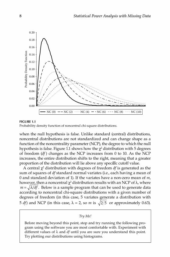
when the null hypothesis is false. Unlike standard (central) distributions, noncentral distributions are not standardized and can change shape as a function of the noncentrality parameter (NCP), the degree to which the null hypothesis is false. Figure 1.1 shows how the χ2 distribution with 5 degrees of freedom (df ) changes as the NCP increases from 0 to 10. As the NCP increases, the entire distribution shifts to the right, meaning that a greater proportion of the distribution will lie above any specific cutoff value.
A central χ2 distribution with degrees of freedom df is generated as the sum of squares of df standard normal variates (i.e., each having a mean of 0 and standard deviation of 1). If the variates have a non‑zero mean of m, however, then a noncentral χ2 distribution results with an NCP of λ, where m df= λ/ . Below is a sample program that can be used to generate data according to noncentral chi‑square distributions with a given number of degrees of freedom (in this case, 5 variates generate a distribution with5 df) and NCP (in this case, λ = 2, so m is 2 5 or approximately 0.63).
Try Me!
Before moving beyond this point, stop and try running the following pro‑gram using the software you are most comfortable with. Experiment with different values of λ and df until you are sure you understand this point. Try plotting our distributions using histograms.
0.00
0.02
0.04
0.06
0.08
0.10
0.12
0.14
0.16
0.18
0.20
Prob
abili
ty D
ensit
y Fu
nctio
n
NC (0) NC (2) NC (4) NC (6) NC (8) NC (10)
Figure 1.1Probability density function of noncentral chi‑square distributions.
Y100315.indb 8 7/15/09 2:58:46 PM

Introduction 9
set seed 17881 ! (We discuss this in Chapter 9)set obs 10000generate ncp = 2generate x1 = invnorm(uniform()) + sqrt(ncp/5)generate x2 = invnorm(uniform()) + sqrt(ncp/5)generate x3 = invnorm(uniform()) + sqrt(ncp/5)generate x4 = invnorm(uniform()) + sqrt(ncp/5)generate x5 = invnorm(uniform()) + sqrt(ncp/5)generate nchia = x1*x1 + x2*x2 + x3*x3 + x4*x4 + x5*x5generate nchib = invnchi2(5,ncp,uniform())summarize nchia nchibclear all
Factors important for Power
Despite being able to trace the origins of interest in statistical power back to the early part of the last century when Neyman and Pearson (1928a, 1928b) initiated the discussion, it is probably Jacob Cohen (e.g., 1969, 1988, 1992) whose work can in large part be credited with bringing statistical power to the attention of social and behavioral scientists. Today it occupies a central role in the plan‑ning and design of studies and interpretation of research results.
Estimating statistical power involves four different parameters: the Type I error rate, the sample size, the effect size, and the power. When the power function is known, it can be solved for any of these parameters. In this way, power calculations are often used to determine a sample size appropriate for testing specific hypotheses in a study. Each of these factors has a pre‑dictable association with power, although the precise relationships can dif‑fer widely depending on the specific context. As always, then, the devil is in the details. First, all else equal, statistical power will be greater with a higher Type I error rate. In other words, you will have a greater chance of finding a significant difference when p = .05 (or .10) than when p = .01 (or .001), and one‑tailed tests are more powerful than two‑tailed tests. Often, scientific convention serves to specify the highest Type I error rate that is considered acceptable. Second, power increases with sample size. Because the precision of our estimates of population parameters increases with sam‑ple size, this greater precision will be reflected in greater statistical power to detect effects of a given magnitude, but the association is nonlinear, and there is a law of diminishing returns. At some sample sizes, doubling your N may result in more than a doubling of your statistical power; at other sample sizes, doubling the N may result in a very modest increase in sta‑tistical power. Finally, power will be greater to detect larger effects, rela‑tive to smaller effects. None of these relationships is linear, and the exact power function rarely has a closed‑form solution and is often difficult to approximate.
Y100315.indb 9 7/15/09 2:58:46 PM
10 Statistical Power Analysis with Missing Data
effect Sizes
Different statistical analyses can be used to represent the same relation‑ship. For example, it is possible to test, obtaining equivalent results in each case, a difference between two groups as a mean difference, a cor‑relation, a regression coefficient, or a proportion of variance accounted for. (See the sample syntax on p. 243 of the Appendix for an illustration.) In much the same way, several different effect size measures have been developed to capture the magnitude of these associations. It is not our goal to present and review all of these; many excellent texts consider them in much greater detail than is possible here (see, for example, Cohen, 1988; Grissom & Kim, 2005; or Murphy & Myors, 2004, for good starting points). However, consideration of a few different effect size measures serves as a useful starting point and orientation to the issues that we will turn to in short order.
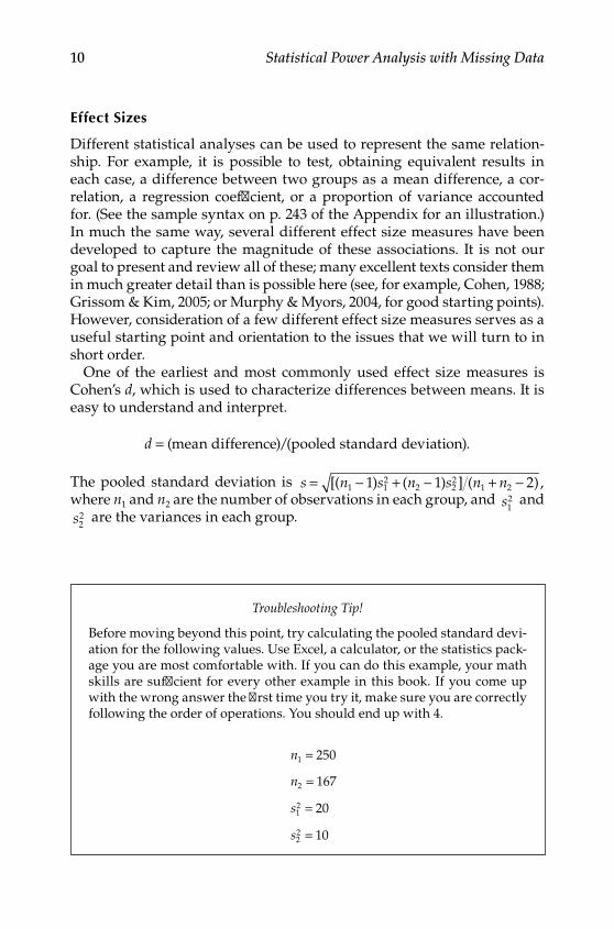
One of the earliest and most commonly used effect size measures is Cohen’s d, which is used to characterize differences between means. It is easy to understand and interpret.
d = (mean difference)/(pooled standard deviation).
The pooled standard deviation is s n s n s n n= − + − + −[( ) ( ) ] ( ) ,1 12
2 22
1 21 1 2 where n1 and n2 are the number of observations in each group, and s1
2 and s2
2 are the variances in each group.
Troubleshooting Tip!
Before moving beyond this point, try calculating the pooled standard devi‑ation for the following values. Use Excel, a calculator, or the statistics pack‑age you are most comfortable with. If you can do this example, your math skills are sufficient for every other example in this book. If you come up with the wrong answer the first time you try it, make sure you are correctly following the order of operations. You should end up with 4.
n
n
s
s
1
2
12
22
250
167
20
10
=
=
=
=
Y100315.indb 10 7/15/09 2:58:47 PM
Introduction 11
Both the mean and the standard deviation are expressed in the same units, so the effect size is unit free. Likewise, the standard deviation is the same, regardless of sample size (for a sample, it is already standardized by the square root of n − 1). In other words, the larger the mean difference relative to the spread of observations, the larger is the effect in question. Beyond relative terms (i.e., larger or smaller effects) for comparing different effects, how we define a small, medium, or large effect is of course fairly arbitrary. Cohen provided guidelines in this regard, suggesting that small, medium, and large effects translated into values of d of .2, .5, and .8, respectively.
Additional commonly used effect size metrics include the correlation coefficient (r), proportion of variance accounted for (i.e., R2), and f2, where the latter is the ratio of explained to unexplained variance (i.e., R2/[1 − R2]). Though a number of formulas are available for moving from one met‑ric to another, they are not always consistent and do not always translate directly. For example, an effect size of .2 corresponds with a correlation of approximately .1. In turn, this corresponds with an R2 value of .01. On the other hand, a large effect size of .8 corresponds with a correlation of approximately .37 and R2 of .14. Cohen, however, describes a large effect size as a correlation of .5 and thus R2 of .25.
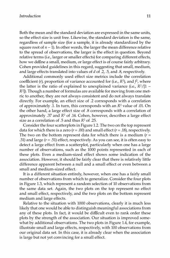
Consider the four scatterplots in Figure 1.2. The two on the top represent data for which there is a zero (r = .00) and small effect (r = .18), respectively. The two on the bottom represent data for which there is a medium (r = .31) and large (r = .51) effect, respectively. As you can see, it is often easy to detect a large effect from a scatterplot, particularly when one has a large number of observations, such as the 1000 points represented in each of these plots. Even a medium‑sized effect shows some indication of the association. However, it should be fairly clear that there is relatively little difference apparent between a null and a small effect or even between a small and medium‑sized effect.
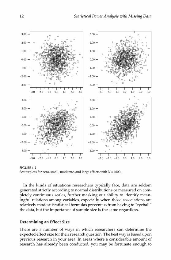
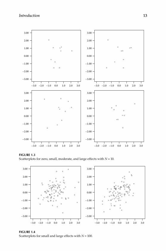
It is a different situation entirely, however, when one has a fairly small number of observations from which to generalize. Consider the four plots in Figure 1.3, which represent a random selection of 10 observations from the same data set. Again, the two plots on the top represent no effect and small effect, respectively, and the two plots on the bottom represent medium and large effects.
Relative to the situation with 1000 observations, clearly it is much less likely that one would be able to distinguish meaningful associations from any of these plots. In fact, it would be difficult even to rank order these plots by the strength of the association. Our situation is improved some‑what by additional observations. The two plots in Figure 1.4, for example, illustrate small and large effects, respectively, with 100 observations from our original data set. In this case, it is already clear when the association is large but not yet convincing for a small effect.
Y100315.indb 11 7/15/09 2:58:48 PM
12 Statistical Power Analysis with Missing Data
In the kinds of situations researchers typically face, data are seldom generated strictly according to normal distributions or measured on com‑pletely continuous scales, further masking our ability to identify mean‑ingful relations among variables, especially when those associations are relatively modest. Statistical formulas prevent us from having to “eyeball” the data, but the importance of sample size is the same regardless.
Determining an effect Size
There are a number of ways in which researchers can determine the expected effect size for their research question. The best way is based upon previous research in your area. In areas where a considerable amount of research has already been conducted, you may be fortunate enough to
3.02.01.00.0–1.0–2.0–3.0
3.00
2.00
1.00
0.00
–1.00
–2.00
–3.00
3.02.01.00.0–1.0–2.0–3.0
3.02.01.00.0–1.0–2.0–3.0 3.02.01.00.0–1.0–2.0–3.0
3.00
2.00
1.00
0.00
–1.00
–2.00
–3.00
3.00
2.00
1.00
0.00
–1.00
–2.00
–3.00
3.00
2.00
1.00
0.00
–1.00
–2.00
–3.00
Figure 1.2Scatterplots for zero, small, moderate, and large effects with N = 1000.
Y100315.indb 12 7/15/09 2:58:49 PM
Introduction 13
3.02.01.00.0–1.0–2.0–3.0
3.00
2.00
1.00
0.00
–1.00
–2.00
–3.00
3.02.01.00.0–1.0–2.0–3.0
3.02.01.00.0–1.0–2.0–3.0 3.02.01.00.0–1.0–2.0–3.0
3.00
2.00
1.00
0.00
–1.00
–2.00
–3.00
3.00
2.00
1.00
0.00
–1.00
–2.00
–3.00
3.00
2.00
1.00
0.00
–1.00
–2.00
–3.00
Figure 1.3Scatterplots for zero, small, moderate, and large effects with N = 10.
3.02.01.00.0–1.0–2.0–3.0
3.00
2.00
1.00
0.00
–1.00
–2.00
–3.00
3.02.01.00.0–1.0–2.0–3.0
3.00
2.00
1.00
0.00
–1.00
–2.00
–3.00
Figure 1.4Scatterplots for small and large effects with N = 100.
Y100315.indb 13 7/15/09 2:58:50 PM

14 Statistical Power Analysis with Missing Data
have a meta‑analysis you can consult (cf. Egger, Davey Smith, & Altman, 2001; Lipsey & Wilson, 1993, 2001). These studies, which pool effects across a wide number of studies, provide an overall estimate of the effect sizes you may expect for your own study and can often provide design advice (e.g., differences in effect sizes between randomized and nonrandomized studies, or studies with high‑risk versus population‑based samples) as well. When available, these are usually the best single source for deter‑mining effect sizes.
In the absence of meta‑analyses, a reasonable alternative is to consult available research on a similar topic area or using similar methodology in order to estimate expected effect sizes. Sometimes, if very little research is available in an area, it may be necessary to conduct pilot research in order to estimate effect sizes. Even when there is no information on the type of preventive intervention that a researcher is planning, data from other types of preventive intervention can provide reasonable expecta‑tions about effect sizes for the current research.
Another alternative is to use generic considerations in order to decide whether an expected effect falls within the general range of a small, medium, or large effect size. Again, previous research and experience can be of value in deciding what size of effect is likely (or likely to be of interest to the researcher and to others). In many areas of research, such as clinical and educational settings, there may also be established effect sizes for the smallest effect size that is likely to be meaning‑ful in practical or clinical terms within a particular context. Does an intervention really have a meaningful effect on employee retention if it changes staff turnover by less than 10%? Is an intervention of value with a population if it works as well as the current best practice (fine, if your intervention is easier or less expensive to administer, is likely to have lower risk of adverse effects, or represents an application to a new population, for example), or does it need to represent an improvement over the state of the art (and if so, by how much in order to represent a meaningful improvement)?
Point estimates and Confidence intervals
Suppose that we randomize 10 people each to our treatment and control groups, respectively. We administer our manipulation (drug versus pla‑cebo, intervention versus psychoeducational control, and valid so forth) and then administer a scale that provides reliable and valid scores to eval‑uate differences between the groups on our outcome variable. We find that our control group has a mean of 10 and our treatment group has a mean of 11. What should we conclude about the efficacy of our treatment or inter‑vention in the population? Obviously, we do not have enough information to reach any conclusion, based on just the group means alone. Though the
Y100315.indb 14 7/15/09 2:58:50 PM

Introduction 15
means provide us with information about point estimates, we also require information about how these scores are distributed (i.e., their variability) in order to be able to make an inference about whether the populations our groups represent differ from one another and, if so, how robust or replicable this difference is.
Consider the following scenario. We have two groups, and the true val‑ues of their means differ by a small, but meaningful amount, say one fifth (d = .2), one half (d = .5), or four fifths (d = .8) of a standard deviation (equiv‑alent to small, medium, and large effects as we discussed above). If we examine the distributions of the raw variables by group, we can see that the larger the difference between means, the easier it is to identify differ‑ence between the two groups. You should notice, however, that there is also a considerable degree of overlap between the two distributions, regardless of the size of the effect. Many times, in fact, particularly with small effects, there is more overlap than difference between groups. The purpose of a carefully planned power analysis is nothing more than to ensure that, if difference or association does exist in the population, the researcher has an acceptable probability of detecting it. Given the difficulties in find‑ings such effects even when they exist, such an analysis is definitely to the researcher’s advantage. For example, the distributions of the reference and small difference distributions in Figure 1.5 overlap fully 42%. For the medium and large effects, the overlaps are 31 and 21%, respectively.
0.0
0.1
0.2
0.3
0.4
–3.0 –2.5 –2.0 –1.5 –1.0 –0.5 0.0 0.5 1.0 1.5 2.0 2.5 3.0
Reference Small Medium Large
Figure 1.5Distributions of variables illustrating small, medium, and large differences.
Y100315.indb 15 7/15/09 2:58:51 PM
16 Statistical Power Analysis with Missing Data
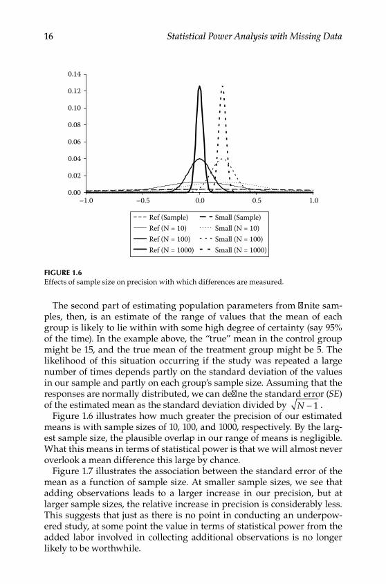
The second part of estimating population parameters from finite sam‑ples, then, is an estimate of the range of values that the mean of each group is likely to lie within with some high degree of certainty (say 95% of the time). In the example above, the “true” mean in the control group might be 15, and the true mean of the treatment group might be 5. The likelihood of this situation occurring if the study was repeated a large number of times depends partly on the standard deviation of the values in our sample and partly on each group’s sample size. Assuming that the responses are normally distributed, we can define the standard error (SE) of the estimated mean as the standard deviation divided by N − 1 .
Figure 1.6 illustrates how much greater the precision of our estimated means is with sample sizes of 10, 100, and 1000, respectively. By the larg‑est sample size, the plausible overlap in our range of means is negligible. What this means in terms of statistical power is that we will almost never overlook a mean difference this large by chance.
Figure 1.7 illustrates the association between the standard error of the mean as a function of sample size. At smaller sample sizes, we see that adding observations leads to a larger increase in our precision, but at larger sample sizes, the relative increase in precision is considerably less. This suggests that just as there is no point in conducting an underpow‑ered study, at some point the value in terms of statistical power from the added labor involved in collecting additional observations is no longer likely to be worthwhile.
0.00
0.02
0.04
0.06
0.08
0.10
0.12
0.14
–1.0 –0.5 0.0 0.5 1.0
Ref (Sample) Small (Sample)Ref (N = 10) Small (N = 10)Ref (N = 100) Small (N = 100)Ref (N = 1000) Small (N = 1000)
Figure 1.6Effects of sample size on precision with which differences are measured.
Y100315.indb 16 7/15/09 2:58:52 PM

Introduction 17
reasons to estimate Statistical Power
Although the origins of statistical power date back more than 80 years to the seminal work of statisticians such as Neyman and Pearson (1928a, 1928b), studies with insufficient statistical power to provide robust answers per‑sist to the present day. Particularly in today’s highly competitive research environment, social science studies are labor intensive to perform, data are difficult and expensive to conduct, and the time‑saving aspects of data entry and analysis afforded by modern computers are often more than offset by the concomitant expectations from journal editors (and gradu‑ate committees) for multiple and complex analyses as well as sensitivity analyses of the data. In the chapters that follow, we build from first prin‑ciples toward a powerful set of applications and tools that researchers can use to better understand the likely effects of missing data on their power to reach valid conclusions.
Conclusions
In this chapter, we provided a review and overview of some of the key concepts related to statistical power with an emphasis on more concep‑tual and intuitive aspects. Each of the next three chapters provides back‑ground in some fundamental principles that will be necessary in order to conduct a power analysis with incomplete data. The next chapter intro‑duces the LISREL model and works through a number of complete exam‑ples of how the same statistical model can be represented graphically, in
0
1
2
3
4
5
6
0 100 200 300 400 500 600 700 800 900 1000
Figure 1.7Effects of increasing sample size on precision of estimates.
Y100315.indb 17 7/15/09 2:58:53 PM

18 Statistical Power Analysis with Missing Data
terms of matrices and in terms of a set of equations. Chapter 3 provides information about missing data and some commonly used strategies to deal with it. Finally, Chapter 4 provides information about four methods for evaluating statistical power with complete data. Each of these chap‑ters builds on the introductory material presented here. You may wish to consult one or more of the additional readings included at the end of each chapter along the way.
Further Readings
Abraham, W. T., & Russell, D. W. (2008). Statistical power analysis in psychological research. Social and Personality Psychology Compass, 2, 283–301.
Cohen, J. H. (1992). A power primer. Psychological Bulletin, 112, 115–159.Grissom, R. J., & Kim, J. J. (2005). Effect sizes for research: A broad practical approach.
Mahwah, NJ: Erlbaum.Murphy, K. R., & Myors, B. (2004). Statistical power analysis: A simple and general
model for traditional and modern hypothesis tests. Mahwah, NJ: Erlbaum.
Y100315.indb 18 7/15/09 2:58:53 PM

ISection
Fundamentals
Y100315.indb 19 7/15/09 2:58:53 PM

Y100315.indb 20 7/15/09 2:58:53 PM
21
2The LISREL Model
LISREL, short for linear structural relations, is both a proprietary software package for structural equation modeling and (in the way we intend it here) a general term for the relations among manifest (observed) and latent (unobserved variables). This very general statistical model encom‑passes a variety of statistical methods such as regression, factor analysis, and path analysis. In this book, we assume that the reader has familiarity with this general class of models, along with at least one software pack‑age for their estimation. Several excellent introductory volumes are avail‑able for learning structural equation modeling, including Arbuckle (2006), Bollen (1989b), Byrne (1998), Hayduk (1987), Hoyle (1995), Kaplan (2009), Kelloway (1998), Raykov and Marcoulides (2006), and Schumacker and Lomax (2004), as well as several others.
Currently, there is a similar profusion of excellent software packages for the estimation of structural equation models, such as LISREL (K. Jöreskog & Sörbom, 2000), AMOS (Arbuckle, 2006), EQS (Bentler, 1995), MPlus (L. K. Muthén & Muthén, 2007), and Mx (Neale, Boker, Xie, & Maes, 2004). Most of these packages have student versions available that permit lim‑ited modeling options, and any of them should be sufficient for nearly all of the examples presented in this volume. Mx is freely available and full featured but places slightly greater demands on the knowledge of the user than the commercial packages. Any statistical package with a reason‑able complement of matrix utilities can also be used for structural equa‑tion modeling, and there are examples in the literature of how they may be implemented in several of them. Fox (2006) illustrates how to estimate structural equation models (currently only for single group models) using the freely available R statistical package, for example, and Rabe‑Hesketh, Skrondal, and Pickles (2004) show how a wide variety of structural equa‑tion models may be estimated using Stata.
Historically, each software package had its own strengths and weak‑nesses, ranging from the generality of the language; whether it was designed for model specification through the use of matrices, equations, or graphical input; the scope of the estimation techniques it provided; and the range of options for output and data structures it could accommodate,
Y100315.indb 21 7/15/09 2:58:53 PM

22 Statistical Power Analysis with Missing Data
such as sampling and design weights. Today, however, the similarities between these packages far outnumber their differences, and this means that a wide range of analytic specifications is available in nearly all of these programs. Originally intended for matrix specification, for exam‑ple, the current version of LISREL also features the SIMPLIS language input in equation form, as well as direct modeling through a graphical interface.
Though we wish to highlight the considerable similarities among the various software packages, we adopt a matrix‑based approach to model specification for most of our examples for a variety of reasons. First, we believe that this approach represents the most direct link between the data structure and estimation methods. Second, it provides a straight‑forward connection between the path diagrams, equations, and syntax. Finally, for the examples that we present, it is most often the simplest and most compact way to move from data to analysis. As a result, only a small amount of matrix algebra is all that is necessary to understand all of the concepts that are introduced in this book, and we review the relevant material here. Readers who have less experience with structural equa‑tion modeling are referred to the sources listed above; those without at least some background in elementary matrix algebra may wish to consult introductory sources such as Fox (2009), Namboodiri (1984), Abadir and Magnus (2005), Searle (1982), or the useful appendices provided in Bollen (1989b) or Greene (2007). For each of the examples that we present in this chapter, we provide equivalent syntax in LISREL, SIMPLIS, AMOS, and MPlus.
Matrices and the LISREL Model
A matrix is a compact notation for sets of numbers (elements), arranged in rows and columns. In matrix terminology, a number all by itself is referred to as a scalar. The most common elements represented within matrices for our purposes will be data and the coefficients from systems of equations. Matrix algebra provides a succinct way of representing these equations and their relationships. For example, consider the following three equa‑tions with three unknown quantities.
x y z
x y z
x y z
+ + =
+ + =
+ + =
2 3 1
4 5 6 4
7 8 9 9
Y100315.indb 22 7/15/09 2:58:54 PM

The LISREL Model 23
We can represent the coefficients of these equations in the following matrix, which we can name A.
A =
1 2 3 14 5 6 47 8 9 9
Individual elements in a matrix are referred to by their row and column position. The element of the second row and the third column in matrix A above (in this case, the number 6) would be referred to as a23. By conven‑tion, matrices are referred to with uppercase letters, whereas their ele‑ments are referred to by lowercase letters.
Most of the operations familiar with scalar algebra (e.g., addition and subtraction, multiplication and division, and roots) have analogs in matrix algebra, allowing us to convey a complex set of associations and opera‑tions compactly. The rows and columns of a matrix are referred to as its order. The matrix above, for example, has order 3 × 4. If we collected infor‑mation from n individuals on p variables, our data matrix would have order n × p.
The order of two matrices must conform to the rules for specific matrix operations. Matrix addition, for example, requires that two matrices have the same order, whereas multiplication requires that the number of col‑umns of the first matrix is the same as the number of rows of the second matrix. For this reason, multiplying matrix A by matrix B may not yield the same results (or even a matrix of the same order) as multiplying matrix B by matrix A, even if they are conformable for both operations. For exam‑ple, if matrix A has order 2 × 3 and matrix B has order 3 × 2, then both AB and BA are possible, but the order of matrix AB would be 2 × 2, whereas the order of matrix BA would be 3 × 3.
Exchanging the order of columns and rows is referred to as transpos‑ing a matrix. The transpose of a 2 × 3 matrix has order 3 × 2, for example. It is commonly used to make two matrices conformable for a particular operation and is usually indicated either with a prime symbol (′) or a superscript letter T. For a square matrix, the “trace” is defined as the sum of diagonal elements of the matrix. Other operations for square matrices include the inverse (the inverse of matrix A is written as A−1), which is the analog of taking the reciprocal of a scalar value because AA−1 = I. We will first make use of the inverse in Chapter 5 to perform operations similar to division using matrices.
The equivalent of taking the square root of a matrix involves finding a matrix L such that A = LL′ and is referred to as a Cholesky decomposition, which we consider in detail in Chapter 9. Also considered in greater detail
Y100315.indb 23 7/15/09 2:58:54 PM

24 Statistical Power Analysis with Missing Data
in Chapter 9 are eigenvectors (V) and eigenvalues (L) that for a matrix A solve the equation ( )A LI V− = 0 . Finally, the determinant of a matrix (the determinant of matrix A is indicated as | |A ) is a scalar value akin to an “area” or “volume” that characterizes the degree of association among variables. When variables are perfectly associated, the area reduces to 0. Matrices with positive determinants are said to be “positive definite,” a property important, for example, in order to calculate the inverse of a matrix. We will first see the determinant later in this chapter and begin using it in power calculations in Chapter 8.
Latent and Manifest Variables
The LISREL model itself has been around for quite some time (e.g., Jöreskog, 1969, 1970, 1978) and allows for estimating and testing a wide variety of models of interest to social scientists. LISREL defines two types of variables, manifest (observed, or y‑variables) and latent (unob‑served, or eta‑variables, η), with various matrices used to link them. Additionally, LISREL distinguishes between exogenous (x‑side) and endogenous (y‑side) variables, a distinction that is not necessary for esti‑mation of the models we consider here, because all models can be esti‑mated using the endogenous (y‑side) of the LISREL model, allowing us to keep our notation slightly more compact. As a result, we will focus on a total of 6 matrices of the 13 matrices included in the full LISREL model (K. G. Jöreskog & Sörbom, 1996). Some authors (e.g., McArdle & McDonald, 1984) have devised an even more compact notation that requires using only 3 matrices (referred to as slings, arrows, and filters). However, a price must be paid for this simplicity in the form of greater computational time (because of increases in the order of the matrix that must be inverted) and greater difficulty in estimation unless good start‑ing values are also provided.
Try Me!
If A =
3 14 15 92 7
and B =
2 7 1 82 8 1 8
, what are the orders (r × c)
of A and B? What is element (2, 2) of A? Of B? What is the order of AB? What is the order of BA?
Y100315.indb 24 7/15/09 2:58:55 PM
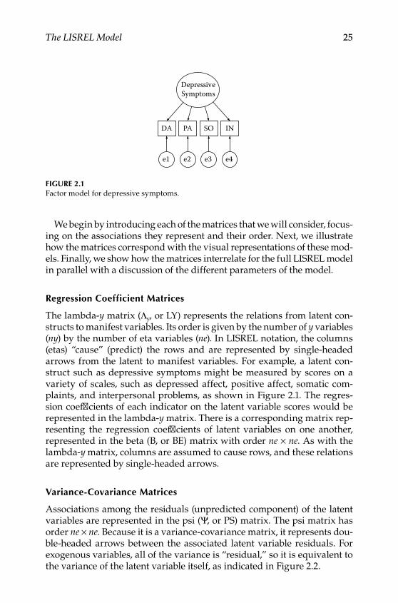
The LISREL Model 25
We begin by introducing each of the matrices that we will consider, focus‑ing on the associations they represent and their order. Next, we illustrate how the matrices correspond with the visual representations of these mod‑els. Finally, we show how the matrices interrelate for the full LISREL model in parallel with a discussion of the different parameters of the model.
regression Coefficient Matrices
The lambda‑y matrix (Λy, or LY) represents the relations from latent con‑structs to manifest variables. Its order is given by the number of y variables (ny) by the number of eta variables (ne). In LISREL notation, the columns (etas) “cause” (predict) the rows and are represented by single‑headed arrows from the latent to manifest variables. For example, a latent con‑struct such as depressive symptoms might be measured by scores on a variety of scales, such as depressed affect, positive affect, somatic com‑plaints, and interpersonal problems, as shown in Figure 2.1. The regres‑sion coefficients of each indicator on the latent variable scores would be represented in the lambda‑y matrix. There is a corresponding matrix rep‑resenting the regression coefficients of latent variables on one another, represented in the beta (B, or BE) matrix with order ne × ne. As with the lambda‑y matrix, columns are assumed to cause rows, and these relations are represented by single‑headed arrows.
Variance‑Covariance Matrices
Associations among the residuals (unpredicted component) of the latent variables are represented in the psi (Ψ, or PS) matrix. The psi matrix has order ne × ne. Because it is a variance‑covariance matrix, it represents dou‑ble‑headed arrows between the associated latent variable residuals. For exogenous variables, all of the variance is “residual,” so it is equivalent to the variance of the latent variable itself, as indicated in Figure 2.2.
DA
e1
PA
e2
SO
e3
IN
e4
DepressiveSymptoms
Figure 2.1Factor model for depressive symptoms.
Y100315.indb 25 7/15/09 2:58:56 PM
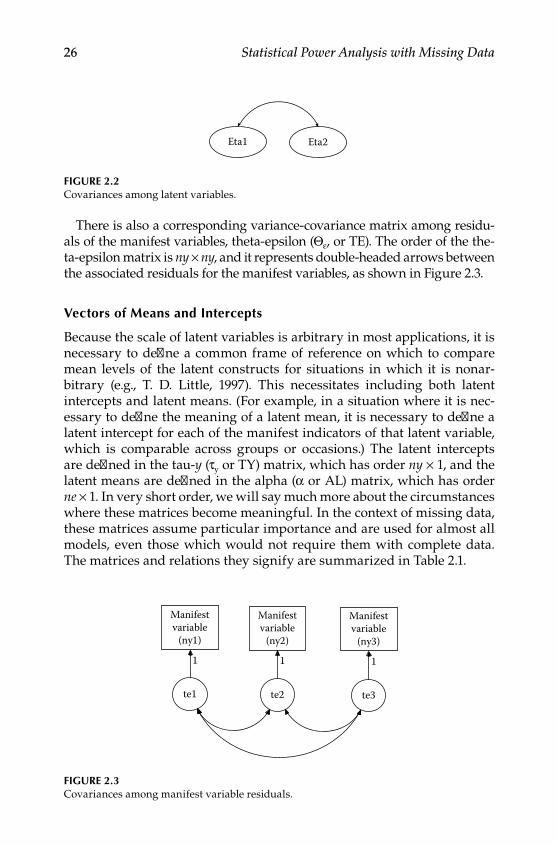
26 Statistical Power Analysis with Missing Data
There is also a corresponding variance‑covariance matrix among residu‑als of the manifest variables, theta‑epsilon (Θε, or TE). The order of the the‑ta‑epsilon matrix is ny × ny, and it represents double‑headed arrows between the associated residuals for the manifest variables, as shown in Figure 2.3.
Vectors of Means and intercepts
Because the scale of latent variables is arbitrary in most applications, it is necessary to define a common frame of reference on which to compare mean levels of the latent constructs for situations in which it is nonar‑bitrary (e.g., T. D. Little, 1997). This necessitates including both latent intercepts and latent means. (For example, in a situation where it is nec‑essary to define the meaning of a latent mean, it is necessary to define a latent intercept for each of the manifest indicators of that latent variable, which is comparable across groups or occasions.) The latent intercepts are defined in the tau‑y (τy or TY) matrix, which has order ny × 1, and the latent means are defined in the alpha (α or AL) matrix, which has order ne × 1. In very short order, we will say much more about the circumstances where these matrices become meaningful. In the context of missing data, these matrices assume particular importance and are used for almost all models, even those which would not require them with complete data. The matrices and relations they signify are summarized in Table 2.1.
Manifestvariable
(ny1)
te1
1
Manifestvariable
(ny2)
te2
1
Manifestvariable
(ny3)
te3
1
Figure 2.3Covariances among manifest variable residuals.
Eta1 Eta2
Figure 2.2Covariances among latent variables.
Y100315.indb 26 7/15/09 2:58:57 PM
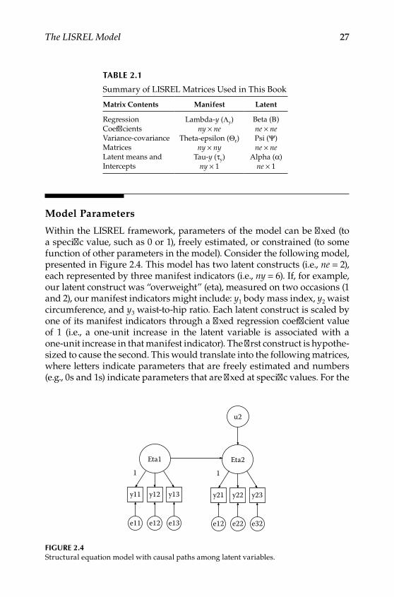
The LISREL Model 27
Model Parameters
Within the LISREL framework, parameters of the model can be fixed (to a specific value, such as 0 or 1), freely estimated, or constrained (to some function of other parameters in the model). Consider the following model, presented in Figure 2.4. This model has two latent constructs (i.e., ne = 2), each represented by three manifest indicators (i.e., ny = 6). If, for example, our latent construct was “overweight” (eta), measured on two occasions (1 and 2), our manifest indicators might include: y1 body mass index, y2 waist circumference, and y3 waist‑to‑hip ratio. Each latent construct is scaled by one of its manifest indicators through a fixed regression coefficient value of 1 (i.e., a one‑unit increase in the latent variable is associated with a one‑unit increase in that manifest indicator). The first construct is hypothe‑sized to cause the second. This would translate into the following matrices, where letters indicate parameters that are freely estimated and numbers (e.g., 0s and 1s) indicate parameters that are fixed at specific values. For the
Table 2.1
Summary of LISREL Matrices Used in This Book
Matrix Contents Manifest Latent
Regression Lambda‑y (Λy) Beta (B)Coefficients ny × ne ne × neVariance‑covariance Theta‑epsilon (Θε) Psi (Ψ)Matrices ny × ny ne × neLatent means and Tau‑y (τy) Alpha (α)Intercepts ny × 1 ne × 1
Eta1
y11
e11
1
y12
e12
y13
e13
Eta2
y21
e12
y22
e22
y23
e32
1
u2
Figure 2.4Structural equation model with causal paths among latent variables.
Y100315.indb 27 7/15/09 2:58:58 PM
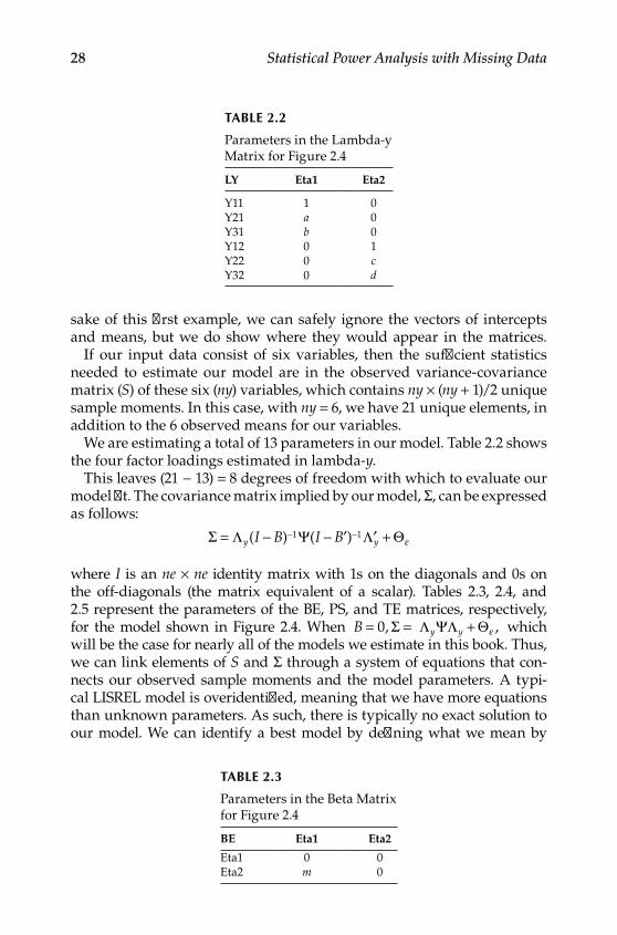
28 Statistical Power Analysis with Missing Data
sake of this first example, we can safely ignore the vectors of intercepts and means, but we do show where they would appear in the matrices.
If our input data consist of six variables, then the sufficient statistics needed to estimate our model are in the observed variance‑covariance matrix (S) of these six (ny) variables, which contains ny × (ny + 1)/2 unique sample moments. In this case, with ny = 6, we have 21 unique elements, in addition to the 6 observed means for our variables.
We are estimating a total of 13 parameters in our model. Table 2.2 shows the four factor loadings estimated in lambda‑y.
This leaves (21 − 13) = 8 degrees of freedom with which to evaluate our model fit. The covariance matrix implied by our model, Σ, can be expressed as follows:
Σ Λ Ψ Λ Θ= − − ′ ′ +− −
y yI B I B( ) ( )1 1ε
where I is an ne × ne identity matrix with 1s on the diagonals and 0s on the off‑diagonals (the matrix equivalent of a scalar). Tables 2.3, 2.4, and 2.5 represent the parameters of the BE, PS, and TE matrices, respectively, for the model shown in Figure 2.4. When B = =0, Σ Λ ΨΛ Θy y + ε , which will be the case for nearly all of the models we estimate in this book. Thus, we can link elements of S and Σ through a system of equations that con‑nects our observed sample moments and the model parameters. A typi‑cal LISREL model is overidentified, meaning that we have more equations than unknown parameters. As such, there is typically no exact solution to our model. We can identify a best model by defining what we mean by
Table 2.2
Parameters in the Lambda‑y Matrix for Figure 2.4
LY Eta1 Eta2
Y11 1 0Y21 a 0Y31 b 0Y12 0 1Y22 0 cY32 0 d
Table 2.3
Parameters in the Beta Matrix for Figure 2.4
BE Eta1 Eta2
Eta1 0 0Eta2 m 0
Y100315.indb 28 7/15/09 2:58:58 PM
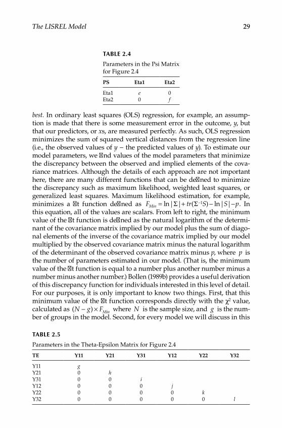
The LISREL Model 29
best. In ordinary least squares (OLS) regression, for example, an assump‑tion is made that there is some measurement error in the outcome, y, but that our predictors, or xs, are measured perfectly. As such, OLS regression minimizes the sum of squared vertical distances from the regression line (i.e., the observed values of y − the predicted values of y). To estimate our model parameters, we find values of the model parameters that minimize the discrepancy between the observed and implied elements of the cova‑riance matrices. Although the details of each approach are not important here, there are many different functions that can be defined to minimize the discrepancy such as maximum likelihood, weighted least squares, or generalized least squares. Maximum likelihood estimation, for example, minimizes a fit function defined as F tr S S pMin = + − −−ln| | ( ) ln| |Σ Σ 1 . In this equation, all of the values are scalars. From left to right, the minimum value of the fit function is defined as the natural logarithm of the determi‑nant of the covariance matrix implied by our model plus the sum of diago‑nal elements of the inverse of the covariance matrix implied by our model multiplied by the observed covariance matrix minus the natural logarithm of the determinant of the observed covariance matrix minus p, where p is the number of parameters estimated in our model. (That is, the minimum value of the fit function is equal to a number plus another number minus a number minus another number.) Bollen (1989b) provides a useful derivation of this discrepancy function for individuals interested in this level of detail. For our purposes, it is only important to know two things. First, that this minimum value of the fit function corresponds directly with the χ2 value, calculated as ( )N g FMin− × where N is the sample size, and g is the num‑ber of groups in the model. Second, for every model we will discuss in this
Table 2.4
Parameters in the Psi Matrix for Figure 2.4
PS Eta1 Eta2
Eta1 e 0Eta2 0 f
Table 2.5
Parameters in the Theta‑Epsilon Matrix for Figure 2.4
TE Y11 Y21 Y31 Y12 Y22 Y32
Y11 gY21 0 hY31 0 0 iY12 0 0 0 jY22 0 0 0 0 kY32 0 0 0 0 0 l
Y100315.indb 29 7/15/09 2:58:59 PM
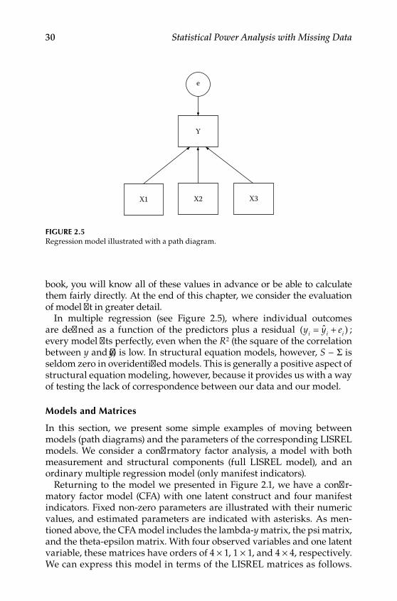
30 Statistical Power Analysis with Missing Data
book, you will know all of these values in advance or be able to calculate them fairly directly. At the end of this chapter, we consider the evaluation of model fit in greater detail.
In multiple regression (see Figure 2.5), where individual outcomes are defined as a function of the predictors plus a residual ( ˆ )y y ei i i= + ; every model fits perfectly, even when the R2 (the square of the correlation between y and y) is low. In structural equation models, however, S − Σ is seldom zero in overidentified models. This is generally a positive aspect of structural equation modeling, however, because it provides us with a way of testing the lack of correspondence between our data and our model.
Models and Matrices
In this section, we present some simple examples of moving between models (path diagrams) and the parameters of the corresponding LISREL models. We consider a confirmatory factor analysis, a model with both measurement and structural components (full LISREL model), and an ordinary multiple regression model (only manifest indicators).
Returning to the model we presented in Figure 2.1, we have a confir‑matory factor model (CFA) with one latent construct and four manifest indicators. Fixed non‑zero parameters are illustrated with their numeric values, and estimated parameters are indicated with asterisks. As men‑tioned above, the CFA model includes the lambda‑y matrix, the psi matrix, and the theta‑epsilon matrix. With four observed variables and one latent variable, these matrices have orders of 4 × 1, 1 × 1, and 4 × 4, respectively. We can express this model in terms of the LISREL matrices as follows.
Y
X2X1 X3
e
Figure 2.5Regression model illustrated with a path diagram.
Y100315.indb 30 7/15/09 2:59:00 PM

The LISREL Model 31
For all symmetric matrices in this section, only the lower triangle is shown, in order to aid in counting the number of estimated model parameters.
Λ Ψ Θy =
= =
100 00 0 0
***
, [*],
**
**
ε
.
To identify the scale of the latent variable, we fix one element of lambda‑y (in this case, element 1,1) equal to 1. This means that a one‑unit increase in the latent variable is associated with a one‑unit increase in this manifest indicator (in other words, they are evaluated on the same scale). Though the actual choice of scaling is arbitrary (that is, any appropriate element of lambda‑y will work), most people recommend using the most reliable indicator. In most cases, you should choose the indicator that makes inter‑pretation of your results most convenient. The input covariance matrix is 4 × 4, with 10 unique elements. The model estimates eight parameters, and so there are 2 degrees of freedom for testing model fit.
Instead of scaling the latent variable as a function of a manifest indicator, we could also fix the variance of the latent construct at some value, typically 1. This would result in just a small change to the model specifications, as follows.
Λ Ψ Θy =
= =
****
, [ ],
**
**
1 00 00 0 0
ε ..
This suggests that a one standard deviation increase in the latent variable is associated with a change in the manifest indicators equivalent to the ele‑ments of lambda‑y. In regression terms, the first situation where scaling is done in lambda‑y is analogous to the unstandardized (b) regression coef‑ficient. This second scaling is analogous to the standardized (β) regression coefficient. Although it is parameterized differently from the preceding model, it is equivalent in the sense that it also estimates eight parameters and provides an equivalent fit to the data. (Note, however, that depending on the software package used to estimate the models, although the over‑all fit will be identical in both parameterizations, the estimated standard errors for individual model parameters may differ from one package to another. See Gonzalez & Griffin, 2001, for a full description of when this is an issue.) Each of the figures shown in this chapter illustrates the associa‑tions among latent and manifest variables graphically in what is referred to as a path diagram or, less commonly, a reticular action model. Properly drawn, these figures can be used to estimate structural equation mod‑els directly in a program such as AMOS, through matrices in a program such as LISREL or Mx, or in equation form in a program such as MPlus,
Y100315.indb 31 7/15/09 2:59:01 PM
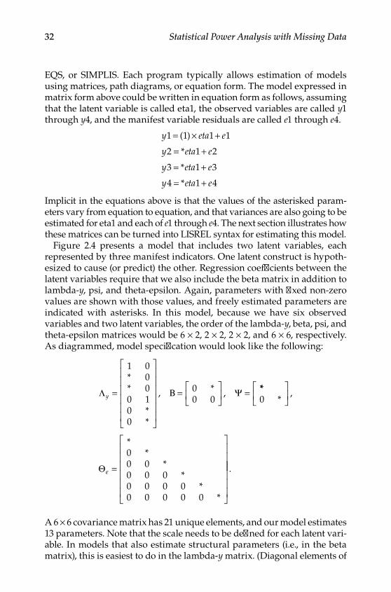
32 Statistical Power Analysis with Missing Data
EQS, or SIMPLIS. Each program typically allows estimation of models using matrices, path diagrams, or equation form. The model expressed in matrix form above could be written in equation form as follows, assuming that the latent variable is called eta1, the observed variables are called y1 through y4, and the manifest variable residuals are called e1 through e4.
y eta e
y eta e
y eta e
y eta e
1 1 1 1
2 1 2
3 1 3
4 1 4
= × +
= +
= +
= +
( )
*
*
*
Implicit in the equations above is that the values of the asterisked param‑eters vary from equation to equation, and that variances are also going to be estimated for eta1 and each of e1 through e4. The next section illustrates how these matrices can be turned into LISREL syntax for estimating this model.
Figure 2.4 presents a model that includes two latent variables, each represented by three manifest indicators. One latent construct is hypoth‑esized to cause (or predict) the other. Regression coefficients between the latent variables require that we also include the beta matrix in addition to lambda‑y, psi, and theta‑epsilon. Again, parameters with fixed non‑zero values are shown with those values, and freely estimated parameters are indicated with asterisks. In this model, because we have six observed variables and two latent variables, the order of the lambda‑y, beta, psi, and theta‑epsilon matrices would be 6 × 2, 2 × 2, 2 × 2, and 6 × 6, respectively. As diagrammed, model specification would look like the following:
Λ Β Ψy =
=
=
1 000
0 100
00 0
**
**
, * , ***
,
**
**
**
0
00 00 0 00 0 0 00 0 0 0 0
=
Θε
.
A 6 × 6 covariance matrix has 21 unique elements, and our model estimates 13 parameters. Note that the scale needs to be defined for each latent vari‑able. In models that also estimate structural parameters (i.e., in the beta matrix), this is easiest to do in the lambda‑y matrix. (Diagonal elements of
Y100315.indb 32 7/15/09 2:59:01 PM
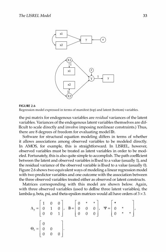
The LISREL Model 33
the psi matrix for endogenous variables are residual variances of the latent variables. Variances of the endogenous latent variables themselves are dif‑ficult to scale directly and involve imposing nonlinear constraints.) Thus, there are 8 degrees of freedom for evaluating model fit.
Software for structural equation modeling differs in terms of whether it allows associations among observed variables to be modeled directly. In AMOS, for example, this is straightforward. In LISREL, however, observed variables must be treated as latent variables in order to be mod‑eled. Fortunately, this is also quite simple to accomplish. The path coefficient between the latent and observed variables is fixed to a value (usually 1), and the residual variance of the observed variable is fixed to a value (usually 0). Figure 2.6 shows two equivalent ways of modeling a linear regression model with two predictor variables and one outcome with the association between the three observed variables treated either as observed or latent constructs.
Matrices corresponding with this model are shown below. Again, with three observed variables (used to define three latent variables), the lambda‑y, beta, psi, and theta‑epsilon matrices would all have orders of 3 × 3.
Λ Β Ψy =
=
=1 0 00 1 00 0 1
00 0 00 0 0
,* *
,**
** *
,
.
00
00 00 0 0
=
Θε
x1
x2
y e
x1
x2
yY1
X21
X11
e
Figure 2.6Regression model expressed in terms of manifest (top) and latent (bottom) variables.
Y100315.indb 33 7/15/09 2:59:02 PM

34 Statistical Power Analysis with Missing Data
Our 3 × 3 input covariance matrix has six unique elements. The model estimates six parameters. Thus, the model fits the data perfectly, as we would expect for a multiple regression model, as discussed in the section above on model parameters.
Structure of a liSrel Program
This section of the chapter works through each of the lines of a typical LISREL program. From there, corresponding syntax for AMOS and MPlus is presented.
It is both good programming form and helpful for documenting each program to begin each program with one or more descriptive title lines. In LISREL, comments can be inserted alone on any line or at the end of any line by using an exclamation point. The first line of a program can also be listed explicitly with the TITLE command. Because it originally adopted FORTRAN conventions, LISREL only requires the first two letters of any command, so TI will also work well.
After the title line or lines, the next line of a LISREL program must spec‑ify the characteristics of the data. The DATA (or DA) line specifies the total number of input variables (NI=), the number of observations (NO=), and the number of groups (NG=), which is needed only if there is more than one group. Two other commonly used options are the data line including the ability to specify a global missing value for list‑wise deletion (XM=) or for full information maximum likelihood (MI=), which we will dis‑cuss in Chapter 3. In simulation studies, it is often useful to run the same model on multiple data sets within a single program, which we will dis‑cuss in Chapter 9, and in this case the number of repetitions (RP=) can be indicated.
Next, variable labels (LA) can be assigned. They can either be read from an external file (FI), such as LA FI=labels.txt, or entered directly in the syn‑tax. (In fact, LA=labels.txt will work just as well.) If they are specified within the program itself, all labels should begin on the line following the LA com‑mand rather than on the same line. If labels are not specified, LISREL will assign them default labels, beginning with VAR1, VAR2, and so forth.
Troubleshooting Tip
Unless a filename or option follows immediately LISREL skips the rest of a line that indicates data will follow. This includes LA as well as lines dis‑cussed below (including CM, LE, RA, etc.). If you accidentally include vari‑able labels or any other input on the same line, it will not be read. Instead, LISREL will look to the following line for this information and your pro‑gram will not be read correctly.
Y100315.indb 34 7/15/09 2:59:02 PM

The LISREL Model 35
Following the labels, the actual input data are specified. LISREL can read data in a variety of forms, most commonly including raw data (RA), covariance matrices (CM), correlation matrices (KM), standard deviations (SD), and means (ME). As with labels, if the data are to be read from an external file, then the file name is specified on the same line specifying the type of data (for example CM=covs.txt or RA=rawdata.dat). If data are to be specified within the program itself, then the command indicating the form of the data is placed on a line by itself, and the data follow beginning on the next line. If a symmetric matrix is being used as input, only the lower triangle is needed. If it is more convenient to specify your data as a full symmetric matrix, then you can add an option to specify that the full (FU) matrix is being provided.
Specifying a model in LISREL is fairly straightforward. It begins with a model (MO) line. This line specifies the number of manifest (NY=) and latent (NE=) variables in the model, and each of the LISREL matrices your model requires, along with the “form” and “mode” for each one. LISREL recognizes a number of common matrix forms, including full (FU, having all unique elements), symmetric (SY, such that element aij = element aji), diag‑onal (DI, with non‑zero elements only on the diagonal), identity (ID, a diag‑onal matrix with 1s on the diagonals), and zero (ZE, with all elements equal to 0) matrices. Several modes are also available. Most commonly, matrices can be specified as having elements that are fixed (FI, initially to a value of 0 by default) or freely estimated (FR). In models with multiple groups, addi‑tional modes include the same pattern of fixed and free elements (SP), the same pattern of fixed and free elements and same starting values (PS), the same starting values only (SS), or invariant (IN) with all elements held equal across groups. For some applications, it is more convenient to initially spec‑ify some matrices as fixed and others as free. However, when first learning to program in LISREL, we recommend specifying all elements as fixed and then explicitly freeing them. Software programs vary considerably in terms of the default values they impose upon a model, so being explicit can help ensure that the model you specified is the one you intended to estimate. This is particularly true with the MPlus software, where the default initial values vary from one type of model to another.
In structural equation modeling, there are three different types of model parameters. A parameter may be fixed (FI) to a specific value (VA), typi‑cally 0 or 1. It may also be freely (FR) estimated. For some models, such as multiple group models, or within a nested sequence of models, one or more parameters may be constrained. Most simply, one parameter may be con‑strained to be equal (EQ) to another parameter. It is also possible to specify linear and nonlinear constraints (CO) such that they are equal to a function of one or more other model parameters. Following the initial model line, the mode of individual model parameters can be specified, provided that it is consistent with the form of the matrix as specified in the model line.
Y100315.indb 35 7/15/09 2:59:02 PM

36 Statistical Power Analysis with Missing Data
In a confirmatory factor model with four manifest indicators and one latent construct, for example, as shown in Figure 2.1, the model line might be as follows:
MO NY=4 NE=1 LY=FU,FI PS=SY,FI TE=SY,FI
First, we would specify the scale of the latent variable, perhaps by using the first manifest indicator.VA 1.0 LY(1,1)
Notice that the specific value appears before the parameter. It is also pos‑sible to specify multiple parameters after this value. Be careful! If the parameter being assigned a value is actually freely estimated within the model, then this value serves only as a starting value, and the parameter will still be freely estimated. We would first have to specify the parameter as fixed with the following syntax:
FI LY(1,1)
To freely estimate the remaining three factor loadings, we would specify the following. (Remember that columns cause rows.)
FR LY(2,1) LY(3,1) LY(4,1)
We would do the same thing for the variance of the latent variable and the residual variances of the manifest indicators.
FR PS(1,1)FR TE(1,1) TE(2,2) TE(3,3) TE(4,4)
We could also have specified it somewhat more efficiently with the follow‑ing model line.
MO LY=FU,FI PS=SY,FR TE=DI,FR
Here we would only have had to free up the remaining three elements of the lambda‑y matrix as we did above. Equality constraints are specified in the same manner. Homoscedastic residuals, for example, can be specified with a single line.
EQ TE(1,1) TE(2,2) TE(3,3) TE(4,4)
In a model with multiple groups, which will often be the case in the situa‑tions considered in this book, it is necessary to specify equality constraints across corresponding parameters in different groups. For example, the
Troubleshooting Tip
We use the passive language that “Y is caused by X” to get the order of rows and columns correct.
Y100315.indb 36 7/15/09 2:59:02 PM

The LISREL Model 37
following syntax would equate residuals in the current group to be equal to the residuals in the first group. The first value refers to the group num‑ber, and the second and third refer to the row and column, respectively.
EQ TE(1,1,1) TE(1,1)EQ TE(1,2,2) TE(2,2)EQ TE(1,3,3) TE(3,3)
Finally, the last line of our program specifies, believe it or not, that we want output (OU). Although a number of options are available with our output, the most important one for our purposes is to specify the number of decimal places we want in our output. For the purposes of power analy‑sis, we usually recommend obtaining our results to at least five decimal places (ND = 5). Other commonly used options include specifying the number of iterations (IT=) and for some nonstandard models where it may be necessary to specify the number of iterations before the admissibility test is performed (AD=) or turn it off completely (AD=OFF). Sometimes, it is necessary to specify NS on the output line, as well. Although it is lightly documented, this tells LISREL to use a method called “steepest descent” to begin minimization instead of its usual approach. When estimating some nonstandard models such as those with missing data, steepest descent works better than LISREL’s default approach. Ordinarily, it is best not to tinker with the defaults unless you run into trouble when estimating your model. Finally, adding the PD command immediately before the output line produces a path diagram in addition to the text output.
Based on the information above, here is what the complete LISREL pro‑gram would look like to estimate the model in Figure 2.4.
! ESTIMATE MODEL FROM FIGURE 2.4DA NI=6 NO=100LAX1 X2 X3 Y1 Y2 Y3CM1.951.20 1.901.40 1.35 1.820.45 0.52 0.65 1.620.50 0.66 0.62 0.98 1.480.61 0.59 0.70 1.18 1.02 1.55MO NY=6 NE=2 LY=FU,FI BE=FU,FI PS=SY,FI TE=DI,FIVA 1.0 LY(1,1) LY(4,2)FR LY(2,1) LY(3,1)FR LY(5,2) LY(6,2)FR BE(1,2)FR PS(1,1) PS(2,2)FR TE(1,1) TE(2,2) TE(3,3)FR TE(4,4) TE(5,5) TE(6,6)OU ND=5
Y100315.indb 37 7/15/09 2:59:02 PM

38 Statistical Power Analysis with Missing Data
In order to maintain continuity, corresponding syntax for AMOS and MPlus is presented at the end of this chapter.
reading and interpreting liSrel Output
Having estimated the model, we next proceed to work through the output it generates. The beginning of the LISREL output includes several pieces of information to ensure that the model and data are being read correctly. The output contains, for example, information about the number of latent and observed variables, along with the sample size.
Number of Input Variables 6Number of Y - Variables 6Number of X - Variables 0Number of ETA - Variables 2Number of KSI - Variables 0Number of Observations 100
Following this, the covariance matrix (and vector of means, if entered) is output. It is important to ensure that the data are being read correctly.
Covariance Matrix x1 x2 x3 y1 y2 y3 ------- ------- ------- ------- ------- -------x1 1.95000x2 1.20000 1.90000x3 1.40000 1.35000 1.82000y1 0.45000 0.52000 0.65000 1.62000y2 0.50000 0.66000 0.62000 0.98000 1.48000y3 0.61000 0.59000 0.70000 1.18000 1.02000 1.55000
After this, the output contains information about the model matrices and which parameters within the matrices are fixed, freely estimated, or
Troubleshooting Tip
Remember to save your syntax file before trying to estimate your model. LISREL simply will not estimate a model for the first time until the syntax file is saved. This is the most common reason why you will not be able to estimate a model in LISREL. Once the model has been saved once, how‑ever, you will be able to estimate it without saving it again. This is the most common reason why you will lose your work when estimating a model in LISREL. Always save your model before trying to estimate it. Finally, we recommend saving your syntax files with the LS8 extension (or SPL if you choose to use the SIMPLIS language). This way LISREL will be sure to rec‑ognize the file every time.
Y100315.indb 38 7/15/09 2:59:02 PM
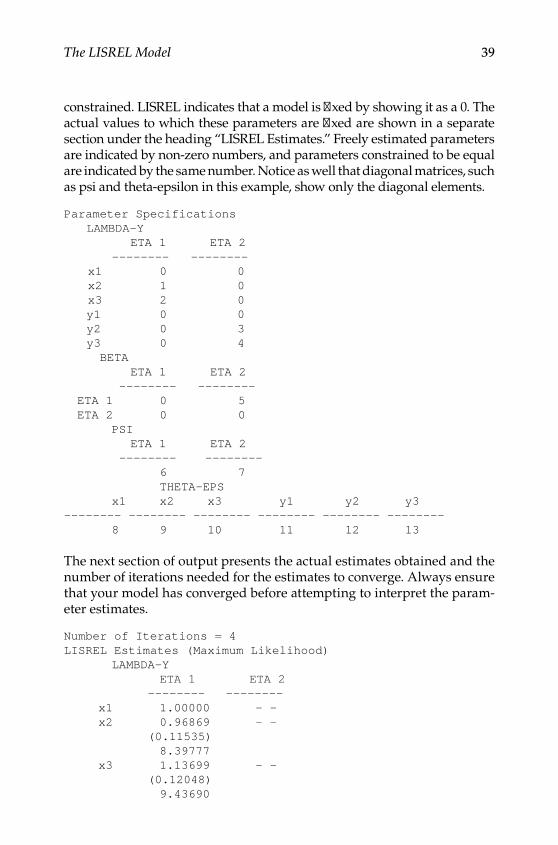
The LISREL Model 39
constrained. LISREL indicates that a model is fixed by showing it as a 0. The actual values to which these parameters are fixed are shown in a separate section under the heading “LISREL Estimates.” Freely estimated parameters are indicated by non‑zero numbers, and parameters constrained to be equal are indicated by the same number. Notice as well that diagonal matrices, such as psi and theta‑epsilon in this example, show only the diagonal elements.
Parameter Specifications LAMBDA-Y ETA 1 ETA 2 -------- -------- x1 0 0 x2 1 0 x3 2 0 y1 0 0 y2 0 3 y3 0 4 BETA ETA 1 ETA 2 -------- -------- ETA 1 0 5 ETA 2 0 0 PSI ETA 1 ETA 2 -------- -------- 6 7 THETA-EPS x1 x2 x3 y1 y2 y3-------- -------- -------- -------- -------- -------- 8 9 10 11 12 13
The next section of output presents the actual estimates obtained and the number of iterations needed for the estimates to converge. Always ensure that your model has converged before attempting to interpret the param‑eter estimates.
Number of Iterations = 4LISREL Estimates (Maximum Likelihood) LAMBDA-Y ETA 1 ETA 2 -------- -------- x1 1.00000 - - x2 0.96869 - - (0.11535) 8.39777 x3 1.13699 - - (0.12048) 9.43690
Y100315.indb 39 7/15/09 2:59:02 PM
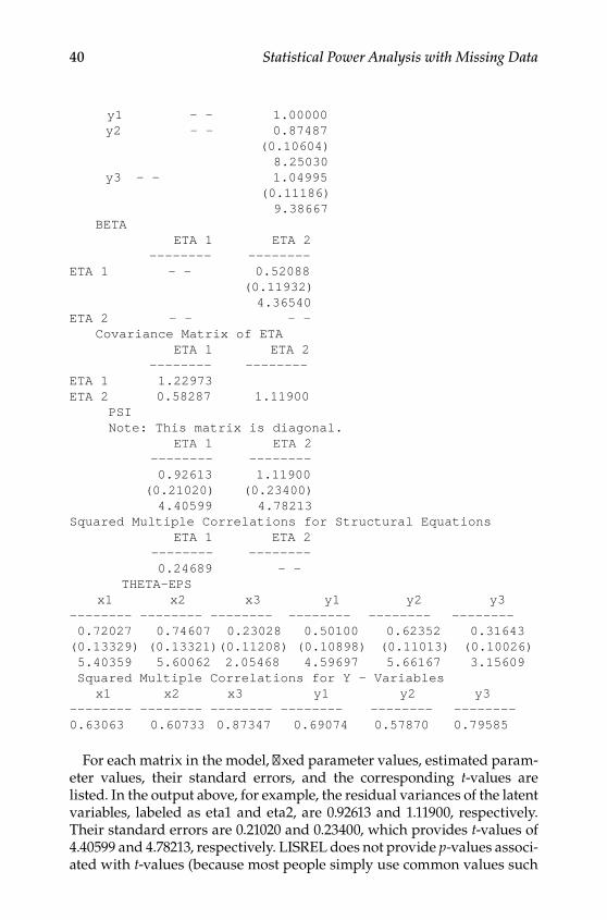
40 Statistical Power Analysis with Missing Data
y1 - - 1.00000 y2 - - 0.87487 (0.10604) 8.25030 y3 - - 1.04995 (0.11186) 9.38667 BETA ETA 1 ETA 2 -------- --------ETA 1 - - 0.52088 (0.11932) 4.36540ETA 2 - - - - Covariance Matrix of ETA ETA 1 ETA 2 -------- --------ETA 1 1.22973ETA 2 0.58287 1.11900 PSI Note: This matrix is diagonal. ETA 1 ETA 2 -------- -------- 0.92613 1.11900 (0.21020) (0.23400) 4.40599 4.78213Squared Multiple Correlations for Structural Equations ETA 1 ETA 2 -------- -------- 0.24689 - - THETA-EPS x1 x2 x3 y1 y2 y3-------- -------- -------- -------- -------- -------- 0.72027 0.74607 0.23028 0.50100 0.62352 0.31643(0.13329) (0.13321)(0.11208) (0.10898) (0.11013) (0.10026) 5.40359 5.60062 2.05468 4.59697 5.66167 3.15609 Squared Multiple Correlations for Y - Variables x1 x2 x3 y1 y2 y3-------- -------- -------- -------- -------- --------0.63063 0.60733 0.87347 0.69074 0.57870 0.79585
For each matrix in the model, fixed parameter values, estimated param‑eter values, their standard errors, and the corresponding t‑values are listed. In the output above, for example, the residual variances of the latent variables, labeled as eta1 and eta2, are 0.92613 and 1.11900, respectively. Their standard errors are 0.21020 and 0.23400, which provides t‑values of 4.40599 and 4.78213, respectively. LISREL does not provide p‑values associ‑ated with t‑values (because most people simply use common values such
Y100315.indb 40 7/15/09 2:59:02 PM
The LISREL Model 41
as ±1.96 to identify statistically significant parameters using a two‑tailed test or ±1.64 for a one‑tailed test). However, you can look up critical values (for your sample size if it is less than about 120) in a table or obtain the val‑ues directly from Excel, SPSS, or some other program. AMOS and MPlus do provide these values automatically.
Additional information such as the squared multiple correlations for observed and latent variables and the covariance matrix of the latent vari‑ables is also provided. In addition to this, LISREL provides a great deal of information concerning model fit, which is discussed in greater detail in the next section.
evaluating Model Fit
Assessment of model fit is one of the most controversial and difficult aspects of structural equation modeling. If there is any consensus in this regard, it is that multiple aspects of model fit need to be considered. This is because there are numerous empirical and philosophical ways in which a model can fit, or fail to fit, observed data. With this recognition, there has been an incredible proliferation in indexes for the assessment of fit. It is clear that no single method is appropriate to determine which model best fits an empirical data set (Gerbing & Anderson, 1993; Hu & Bentler, 1995; McDonald & Marsh, 1990; Mulaik et al., 1989). Rather, it is only through the application of multiple indexes of fit, each with its own strengths and weaknesses, that the satis‑factory fit of a particular model can be determined. Among the most com‑monly applied measures of model fit are those of discrepancy from estimated population values, such as model chi‑square; incremental fit indexes, in which fit of a selected model is assessed against one or more alternative mod‑els; parsimony‑based fit indexes; absolute fit indexes; and considerations of where a model fails to reproduce elements of the observed sample moments. Below, we briefly discuss the most widely used approaches to fitting struc‑tural equation models, along with a discussion of their respective strengths and limitations. Some indexes of fit are based on the assumption that the model being tested is correct, whereas others are not. For this reason, we con‑sider both models that are correct and models that are misspecified to assess performance of fit indexes under various conditions of incomplete data.
Try Me!
Once you get the file above running, rewrite it to scale the first latent variable to have a variance of 1 in psi, estimating all factor loadings for it in lambda‑y. Write the same model with correlated latent variables instead of a causal path in the beta matrix (i.e., PS=SY,FR and BE=ZE). We strongly recommend that you stop here to run this program in the software of your choice before mov‑ing to the next section, which runs through the output provided by LISREL.
Y100315.indb 41 7/15/09 2:59:02 PM
42 Statistical Power Analysis with Missing Data
Measures of Population Discrepancy
The chi‑square statistic (χ2) is by far the most universally reported index of fit in structural equation modeling. Tests of model fit, such as the χ2 test, assess the “magnitude of the discrepancy” (Hu & Bentler, 1995, p.77) between the sampled and modeled or fitted covariance matrices (i.e., |S − Σ|, a test of exact fit). A nonsignificant χ2 with associated degrees of freedom indicates that the two matrices (the observed, S, and the implied, Σ) do not differ statistically and is generally indicative of a good model fit. The χ2 statistic is a linear function of sample size times the minimum value of the fit function. As sample size increases, even very minor mis‑specifications can lead to poor model fit. Conversely, with small samples, models will tend to be accepted even in the face of considerable misspeci‑fication (Schumacker & Lomax, 2004).
Incremental Fit Indices
Model comparison indexes use measures of population discrepancy between the model of interest and some baseline model to assess “rela‑tive” model fit (La Du & Tanaka, 1995). The independence or null model is typically specified as the baseline model, in which there are no associa‑tions being modeled among the variables. Thus, a model of interest can be tested against a poorly fitting independence model to gain perspective on the relative fit of a particular model (Bentler & Bonett, 1980; Tucker & Lewis, 1973).
There are three broad classes of fit indexes based upon comparison to a baseline model (in this case, an independence model). The normed fit index (NFI; Bentler & Bonett, 1980) is an example of a Type 1 (normed) incremental fit index (Hu & Bentler, 1995). It calculates the proportion reduction in chi‑square of the model of interest, relative to a model of no association. Despite being easily interpreted and standardized for all models to lie between 0 and 1, previous research has illustrated several shortcomings of the NFI, the most central of which is its dependence on sample size (Marsh, Balla, & Hau, 1996). All else equal, values of the NFI will be higher for larger sample sizes.
A second comparative fit index is the Tucker‑Lewis index (TLI; Tucker & Lewis, 1973), an example of a Type 2 (nonnormed) incremental fit index. It has been modified from its original use in factor analysis for application to structural equation modeling (Bentler & Bonett, 1980). Unlike the NFI, values of the TLI (also referred to as the NNFI and as ρ) can exceed 1.0. In such circumstances, they are simply truncated to a value of 1.0. The TLI is not associated with sample size.
Finally, Type 3 (noncentrality based) incremental fit indices such as the comparative fit index (CFI; Bentler, 1990) are normed between values of 0 and 1 and are also independent of sample size.
Y100315.indb 42 7/15/09 2:59:03 PM

The LISREL Model 43
Absolute Fit Indices
Most researchers acknowledge that their models, at best, only approximate reality and that even models that are only approximately true can still have considerable value. Under this perspective, a model, like a horseshoe, may be “close enough.” As a measure of the lack of the fit of a model, the root mean square error of approximation (RMSEA) is judged by a value of 0.05 or less as an indication of a close fit of the model in relation to the degrees of freedom; additionally, a value of 0.08 or less is indicative of a “reason‑able” error of approximation such that a model should not be used if it has an RMSEA greater than 0.1 (Browne & Cudeck, 1993). More recently, Hu and Bentler (1995) suggested that values below .06 indicate good fit. LISREL also provides a test that the confidence interval around the RMSEA includes zero. It is worth noting that by default this test is set at a p‑value of .10 rather than the value of .05 more commonly used for other tests.
LISREL provides a wide array of indices of model fit. The one that will be most important in power analysis is the minimum value of the fit function (FMin). For the example estimated above, this value (to 5 digits) is 0.062315. It is related to the minimum fit function chi‑square value as a function of N − 1 (in this case 99). Because this value is independent of sample size, we can use it to estimate a quantity useful for power analyses, a topic we will consider in much greater detail in Chapter 4.
Conclusions
The LISREL model allows for estimation of a wide set of statistical mod‑els including both manifest and latent variables. In this chapter, we have worked through the process of going from a diagrammed model to speci‑fying the structure and content of LISREL matrices. We then discussed the process of turning these matrices into LISREL syntax files, along with a brief presentation of the key components of the output file and issues in assessing model fit. The subsequent appendix provides corresponding syntax for MPlus and AMOS. In the next chapter, we move on to consider issues presented by missing data.
Further Readings
Bollen, K. A. (1989). Structural equations with latent variables. New York: Wiley.Boomsma, A. (2000). Reporting analyses of covariance structures. Structural
Equation Modeling, 7, 461–483.Byrne, B. M. (1998). Structural equation modeling with LISREL, PRELIS, and SIMPLIS:
Basic concepts, applications, and programming. Mahwah, NJ: Erlbaum.
Y100315.indb 43 7/15/09 2:59:03 PM
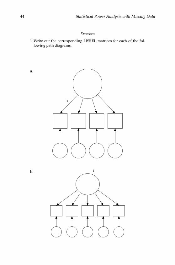
44 Statistical Power Analysis with Missing Data
Exercises
1. Write out the corresponding LISREL matrices for each of the fol‑lowing path diagrams.
1
1b.
a.
Y100315.indb 44 7/15/09 2:59:03 PM
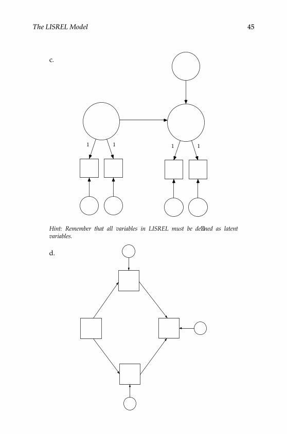
The LISREL Model 45
1 1 1 1
Hint: Remember that all variables in LISREL must be defined as latent variables.
c.
d.
Y100315.indb 45 7/15/09 2:59:04 PM

46 Statistical Power Analysis with Missing Data
2. Draw a path diagram from the following matrices:
Λ Ψ Θy =
=
1 01 00 10 1
2 0 1 61 6 4 0
, . .. .
, ε ==
=
0 7 0 0 00 0 7 0 00 0 1 4 00 0 0 1 4
..
..
****
Λy
= =
, [ ],
**
**
Ψ Θ1
0 0 00 0 00 0 00 0 0
ε
=
=Λ Βy
1 0 00 0
0 00 1 00 0 10 0
0 0*
*
*
,00
0 00 0
0 00 00 0
0 0 0
**
**
*,
*
=
=Ψ Θε
00 00 0 0 0 00 0 0 0 00 0 0 0 00 0 0 0 00 0 0 0 0
**
**
*
3. Write syntax for each of the models above using an identity matrix as the input covariance matrix.
d.
c.
b.
a.
Y100315.indb 46 7/15/09 2:59:04 PM

47
3Missing DataAn Overview
Why Worry About Missing Data?
In many disciplines, missing data are relatively uncommon and often taken as an indicator of sloppy science or poor methodology, and as a result techniques for dealing with missing data when they occur are gen‑erally frowned upon in these areas. In a conversation about dealing with missing data in a large interdisciplinary project, one of our colleagues, a geneticist, sarcastically remarked “All of our subjects had DNA.” Less than 2 weeks later, however, many of the laboratories at his institution were under several feet of water as a result of a hurricane. Fortunately, we had backup samples in multiple sites, his laboratory was on a higher floor of the building, and liquid nitrogen backup systems that required no external power source kept samples frozen until they could be rescued. Subsequent discussions regarding treatment of missing data have been better received.
In the social sciences, however, missing or incomplete data are a nearly ubiquitous aspect of research. Data collection from human beings in the real world poses considerably greater challenges than in the laboratory setting. Participants have other commitments, they move, they become sick or die, they may not wish to provide information of a sensitive nature, and any num‑ber of random or systematic forces may prevent data from being observed.
There is growing recognition that failure to address issues of missing data can lead to biased parameter estimates and incorrect standard errors (Arbuckle, 1996; R. J. A. Little & Rubin, 1989; Schafer, 1997). Techniques for estimation of parameters and their standard errors under conditions of incomplete data have been reported in the structural equation mod‑eling literature for more than two decades (Allison, 1987; B. O. Muthén, Kaplan, & Hollis, 1987). Likewise, the theoretical underpinnings of these approaches are 50 years old (T. W. Anderson, 1957). It is only recently,
Y100315.indb 47 7/15/09 2:59:04 PM
48 Statistical Power Analysis with Missing Data
however, that analyses that incorporate incomplete observations have become commonplace in the social sciences.
There are several reasons why researchers should be concerned with missing data. First, data are difficult to collect, and so researchers should use every piece of information they collect. Second, failing to adequately address issues of missing data can lead to biased results and incorrect conclusions. Finally, studies with missing data are more common than studies without them. Therefore, researchers should know what their best available options are in the very likely event that their study will involve missing data.
In this chapter, we consider several different ways in which data can be missing, along with the different implications this has for analysis of the observed data. We also consider and evaluate several of the avail‑able approaches for handling incomplete data. Finally, we present some worked examples of how incomplete data can be analyzed using struc‑tural equation modeling software.
Types of Missing Data
Missing Completely at random
In their seminal work on the analysis of incomplete data, R. J. A. Little and Rubin (2002) distinguished between three types of missing data. Data are said to be missing completely at random (MCAR) when the probability that an observation is missing (r) does not depend on either the observed (yobs) or the unobserved (ymiss) values. Mathematically, this can be expressed as Pr( | , ) Pr( )r y y robs miss = . In other words, the probability that an observa‑tion is missing is not associated with any variables you have measured or with any variables that are not measured. For this reason, MCAR data are equivalent to a simple random sample of the full data set. It is what most people think of when they say that the data are randomly missing.
Under most circumstances, it is probably fairly unrealistic to assume that data are MCAR (for exceptions, see Graham, Taylor & Cumsille, 2001, and Chapter 8). Rather, under many circumstances, there may be selec‑tive (i.e., systematic) processes that determine the probability that a par‑ticular value will be observed or missing. For example, individuals with extremely high incomes may be less likely to report income information. Similarly, individuals who are geographically mobile may be more dif‑ficult to track and thus more likely to drop out of a longitudinal study. Table 3.1 illustrates some examples of scenarios where data are known to be (or likely to be) MCAR.
Y100315.indb 48 7/15/09 2:59:05 PM

Missing Data 49
Missing at random
A more realistic assumption under these circumstances is that data are missing at random (MAR), that the probability that an observa‑tion is missing depends only on the values of the observed data. In other words, Pr( | , ) Pr( | )r y y r yobs miss obs= . That is, the probability that an observation is missing is completely accounted for by variables that you have measured and nothing that you have not measured. Under circumstances where data are MCAR or MAR, the mechanism that determines whether a particular value is observed or missing is said to be ignorable.
Whereas it is possible to test whether data are MCAR, it is not typically possible to test whether the data are MAR because to do so would require further information about the unobserved data. Even when the data are not strictly MAR, this assumption will often represent a reasonable approxi‑mation (see R. J. A. Little & Rubin, 2002; Molenberghs & Kenward, 2007; or Schafer, 1997, for a more thorough explication of data that are MAR) and is less stringent than the assumption that data are MCAR. Thus, any attempt to identify and correct for selective nonresponse will typically represent an improvement in the accuracy of results over making no attempt at all. Table 3.2 illustrates some examples of scenarios where data are known to be (or likely to be) MAR.
Missing Not at random
In situations where the probability that an observation is missing depends on the values of the unobserved variables, the data are said to be missing not at random (MNAR). Under these circumstances, the nonre‑sponse is said to be informative. Mathematically, this can be expressed as Pr( | , ) Pr( | )r y y r yobs miss miss= . That is, the probability that an observation is missing depends on something that you have not measured (and perhaps things that you have measured as well). Though strategies for dealing with
Table 3.1
Scenarios Where Data Are Likely (or Known) to Be Missing Completely at Random (MCAR)
Scenario Description
1 An investigator randomly assigns students to one of multiple forms of a test she is developing. Each form has some overlapping and some unique items
2 A researcher is collecting short‑term daily diary data from the residents of an island accessible only by a ferry that does not run in foggy weather
3 A printing error results in some pages of a testing booklet being missing for a subset of study participants
4 A subset of participants in a large survey are randomly selected to participate in an in‑depth testing module
Y100315.indb 49 7/15/09 2:59:05 PM

50 Statistical Power Analysis with Missing Data
MNAR data are growing, their analysis always requires some explicit and untestable assumptions about the nature of the unobserved values and the processes underlying them (i.e., the probability that a response is missing depends on ymiss, which by definition is unobserved). In these sit‑uations, many researchers recommend a series of sensitivity analyses in order to evaluate the extent to which results depend on the assumptions being made (cf. Hedeker & Gibbons, 1997; Molenberghs & Kenward, 2007; Schafer & Graham, 2002). Table 3.3 illustrates some examples of scenarios where data are known to be (or likely to be) MNAR.
Table 3.2
Scenarios Where Data Are Likely (or Known) to Be Missing at Random (MAR)
Scenario Description
1 Students with higher math and verbal performance scores, measured for all students, are more likely to be in class on the day of testing
2 Responses during the first part of a telephone survey are used to determine which follow‑up questions are asked
3 Individuals with lower household incomes as measured at baseline are more likely to be lost to follow‑up
4 Older adults who are initially more physically frail are more likely to have died between interviews
Table 3.3
Scenarios Where Data Are Likely (or Known) to Be Missing Not at Random (MNAR)
Scenario Description
1 Individuals with higher (or lower) household incomes are less likely to provide income data
2 Individuals who experience adverse effects of treatment between waves are more likely to be lost to follow‑up
3 Individuals are less likely to return for a follow‑up interview if they experience a depressive episode between visits
4 An interviewer works more vigorously to retain participants who appear to be gaining the most benefit from an intervention (or less vigorously to retain those who do not)
Point of Reflection
In addition to the examples of MCAR, MAR, and MNAR data provided, take a few moments to consider missing data within your own area of research. Can you think of examples of data that would fall into each category? What are some variables that are likely to be associated with the probability that an observation is missing? Are these variables typically measured in stud‑ies in your area?
Y100315.indb 50 7/15/09 2:59:05 PM
Missing Data 51
Strategies for Dealing With Missing Data
Numerous methods are available for dealing with missing data, each with its own strengths and limitations. Following R. J. A. Little and Rubin (2002), we present the approaches according to whether they rely on anal‑ysis of complete cases, available cases, or imputation approaches. Ideally, we seek parameter estimates that are both unbiased (i.e., neither consis‑tently overestimated nor underestimated) and efficient (i.e., estimated as precisely as possible).
Complete Case Methods
As the name suggests, complete case methods make use of only cases hav‑ing complete data on all variables of interest in the analysis. All informa‑tion from cases with incomplete data is ignored.
list‑Wise Deletion
List‑wise deletion, the removal of cases that are missing one or more data points, is by far the most commonly employed method for dealing with missing data. This approach is valid for point estimates only when the data are MCAR but will otherwise lead to biased estimates. For confi‑dence intervals, however, list‑wise deletion is always inefficient (i.e., your standard errors will always be larger), because information from par‑tially observed cases is discarded. Thus, the list‑wise deletion approach to missing data is easy to implement but can yield seriously misleading estimates. Further, in the example we present later in this chapter, the use of list‑wise deletion would result in loss of more than half of the sample (some due to dropout, some due to nonresponse within survey waves), making methods for dealing with incomplete data preferable for reasons of both statistical power and correcting bias in parameter estimates and confidence intervals.
list‑Wise Deletion With Weighting
In addition to simply using all complete cases, there are numerous approaches that give some cases more “weight” than others in the analysis in an attempt to reduce bias due to systematic processes associated with nonresponse. If nonresponse is twice as likely among men as women, data from each man in the sample could receive a weight of 2 in order to make the data more representative. Another approach treats the probabil‑ity of nonresponse as an omitted variable, which results in a specification error in the estimation model (e.g., Heckman, 1979). To adjust for this, the
Y100315.indb 51 7/15/09 2:59:05 PM

52 Statistical Power Analysis with Missing Data
predicted probability of nonresponse for each case is estimated, and the inverse of this variable is included as an additional variable in the model.
available Case Methods
In contrast to complete case methods, available case methods make use of information from both completely and partially observed cases. If a case provides information about pretest scores, but not follow‑up scores, the pretest information is incorporated into the analysis (remember our dis‑cussion of Solomon’s four‑group design in Chapter 1). Because they typi‑cally make use of more information than complete case methods, available case methods are generally better at correcting for bias as a function of selective nonresponse with MAR data than complete case methods.
Pair‑Wise Deletion
After list‑wise deletion, pair‑wise methods are next most commonly used. In pair‑wise deletion, all sample moments (i.e., means, variances, covari‑ances) are calculated on the basis of all cases that are available for a pair of variables. Though this may seem like a good idea in principle, it is fraught with potential inconsistencies, and its use is rarely justified in practice. For example, if the covariance between two variables, X and Y, is given by the formula ∑ =
− −−i
n X X Y YN
i i1 1
( )( ), which means should be used for X and Y ? Should the mean for all available cases of X be used, or should it be calculated as the mean of all cases for which both X and Y are observed? Thus, differ‑ent means may be used to generate each correlation in a matrix. Currently, different statistical packages may calculate pair‑wise covariances using different formulas and so may yield different results for what is ostensibly the same correlation. In addition, it is unlikely that a pair‑wise approach will correctly adjust parameter estimates and standard errors. Without stronger statistical justification, this approach is probably best avoided in statistical analysis.
expectation Maximization algorithm
The expectation maximization (EM) algorithm (Dempster, Laird, & Rubin, 1977) uses a two‑step iterative process to make use of information from all cases, complete and incomplete, in order to estimate sample moments such as means, variances, and covariances. In the first (expectation, or E) step, missing values are replaced with their expected values conditional on the other variables in the model. In the second (maximization, or M) step, maximum likelihood estimates of the means and covariances are obtained as though the expected values were the missing values. These new means
Y100315.indb 52 7/15/09 2:59:06 PM

Missing Data 53
and covariances are used to generate the next iteration’s expected values and the cycle continues until it has converged to the desired degree of pre‑cision (i.e., the difference in estimates between successive iterations is suf‑ficiently small). Use of the EM‑generated covariance matrix can correct for the bias in parameter estimates when data are MAR, but it is impossible to know what (parameter‑ and model‑specific) sample size will yield the correct confidence intervals. In partial response to this limitation, Meng and Rubin (1991) have developed the supplemented EM (SEM) algorithm, which can provide estimates of the asymptotic variance‑covariance matrix, but this approach has not yet been widely implemented in statistical pack‑ages. However, because the EM algorithm is model based, the results still depend in part on which variables are included in the model. R. J. A. Little and Rubin (2002) have also shown how the resampling technique of boot‑strapping (e.g., Efron & Tibshirani, 1993) can be used to obtain standard errors for EM‑generated estimates.
Full information Maximum likelihood
The idea behind full information maximum likelihood (FIML) originates with T. W. Anderson (1957), who discovered that, under nested missing data structures (e.g., when individuals who are missing at one wave of data col‑lection are missing at all subsequent waves), the resulting likelihood func‑tion could be factored separately for each pattern of missing data. The EM algorithm above allowed for solving otherwise intractable problems (i.e., where no closed‑form solution exists or would be exceedingly difficult to specify or solve) via iterative methods and was largely responsible for the widespread application of Anderson’s methods. Initial estimates of model parameters (based, for example, on estimates from list‑wise or pair‑wise deletion) are optimized over all available information from complete and partial cases. These new estimates are then substituted back in for the model parameters, and the optimization process continues in this fash‑ion until the parameter estimates converge. An extension of this approach, FIML, can recover correct parameter estimates and confidence intervals under both MCAR and MAR conditions. FIML maximizes the function χ µMin i
Ni mm i
Ni m i m i mmy2
1 11= ∑ + ∑ − ′= =
−log| | ( ) (, , , ,Σ Σ yyi m i m, , )− µ on a case‑wise basis, where yi,m represents the observed data for case i, and μi,m and Σi,mm are the means and covariances of observed data for case i (e.g., Arbuckle, 1996; Jamshidian & Bentler, 1999). You should notice a strong similarity between the structure of this equation and the discrepancy function introduced in Chapter 2. In essence all model parameters that can be estimated from an observation are used to construct a weighted average across patterns of missing data, something that we will demonstrate, in simplified fashion, below. This approach has been incorporated into statistical software pack‑ages such as AMOS (Arbuckle, 2006; Wothke, 1998), MPlus, Mx, and LISREL.
Y100315.indb 53 7/15/09 2:59:06 PM
54 Statistical Power Analysis with Missing Data
Even when data are only MAR, FIML makes use of all available data, even those from partially missing cases, and will provide valid point estimates and confidence intervals for population parameters. However, because it is also a model‑based technique, estimates of the same parameters and their confidence intervals may vary from analysis to analysis, depending on which other variables are included in the model.
Imputation Methods
One meaning of imputation is to assign an attribute based on similarity to something else. In contrast to the complete case methods, which use only cases with complete data, and available case methods, which use only data values actually observed, imputation methods involve the replacement of unobserved (i.e., missing) values with hypothetical data. Another mean‑ing of imputation has to do with assignment of fault or responsibility. Perhaps for this reason, and perhaps also because of longstanding taboos against making up data, it has taken some time for imputation methods to gain general favor in the social sciences even though these methods are at least as sound as other approaches that have been more acceptable for a longer period of time.
Single imputation
Single imputation is another useful technique when data are MAR and involves replacing missing data with plausible values, which can be derived in any of a number of ways (e.g., substitution of values from a complete case with similar values on the observed variables, or more sophisticated Bayesian methods). The result is a rectangular data matrix that is amenable to analysis with standard statistical software and param‑eter estimates will be consistent from one model to another.
There are a variety of methods to fill in missing values. Substitution of the mean for missing values is one approach that is used quite com‑monly, but it will only result in unbiased parameter estimates if data are MCAR. Similarly, substitution of predicted values from a regression equa‑tion is another commonly used approach that fares slightly better. Other approaches use values from completely observed cases with similar values on the variables that are observed for both cases. If the missing values are selected from a random sample of similar cases, the result is hot‑deck impu‑tation. If instead the missing values are always filled in with the same new values, then the result is termed cold‑deck imputation (and variance will be
Y100315.indb 54 7/15/09 2:59:06 PM

Missing Data 55
reduced similarly to the method of mean substitution). Bayesian methods are also available to generate the plausible values of missing data.
A single imputation will provide valid point estimates, but the associ‑ated standard errors will be too small. The imputation process naturally involves some uncertainty about what the unobserved values were, but this uncertainty is not reflected anywhere in the data matrix. As a result, this technique, like mean or regression substitution, leads to an undesir‑able overestimate of the precision of one’s results. Multiple imputation, discussed next, represents one way of correcting for the uncertainty inherent in the process of imputation.
Multiple imputation
For both MAR and MCAR data, multiple imputation (MI) combines the strengths of FIML and single imputation in that it provides valid point estimates and confidence intervals along with a collection of rectangular data matrices that can be used for the analysis of many different models. Additionally, the fact that missing data are replaced with multiple plausible values provides the analyst with valid confi‑dence intervals in the following fashion. Within any data set, there will always be some uncertainty about population parameters due to sampling variability.
With incomplete data, some uncertainty is also introduced through the process of imputation. However, when multiple data sets are imputed, the only source of variability in parameter estimates across them is due to uncertainty from the imputation process (because the complete data com‑ponents are identical across data sets). Thus, by decomposing the total variability in parameter estimates into within‑imputation variability and between‑imputation variability, the results can be accurately corrected for the uncertainty introduced through the imputation process.
Schafer has recently written a software package, NORM, to perform multiple imputation and form valid inferences (described in Schafer, 1997; see also Graham, Olchowski, & Gilreath, 2007) under a normal model, making this technique readily available to social scientists without the technical expertise to implement MI themselves (other imputation mod‑els now becoming available are useful for categorical and mixed models). This is a highly generalized approach to missingness that can be used in conjunction with many statistical procedures, including, for example, structural equation models and logistic regression equations. Multiple imputation is statistically sound and empirically useful in a wide variety of contexts. Its application is slightly more complicated within a structural equation modeling framework, however (Davey, Savla, & Luo, 2005; Meng & Rubin, 1992), and so we do not consider this approach further here.
Y100315.indb 55 7/15/09 2:59:06 PM
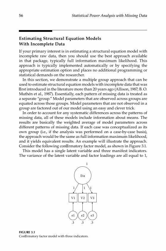
56 Statistical Power Analysis with Missing Data
Estimating Structural Equation Models With Incomplete Data
If your primary interest is in estimating a structural equation model with incomplete raw data, then you should use the best approach available in that package, typically full information maximum likelihood. This approach is typically implemented automatically or by specifying the appropriate estimation option and places no additional programming or statistical demands on the researcher.
In this section, we demonstrate a multiple group approach that can be used to estimate structural equation models with incomplete data that was first introduced in the literature more than 20 years ago (Allison, 1987; B. O. Muthén et al., 1987). Essentially, each pattern of missing data is treated as a separate “group.” Model parameters that are observed across groups are equated across those groups. Model parameters that are not observed in a group are factored out of our model using an easy and clever trick.
In order to account for any systematic differences across the patterns of missing data, all of these models include information about means. The results are basically the weighted average of model parameters across different patterns of missing data. If each case was conceptualized as its own group (i.e., if the analysis was performed on a case‑by‑case basis), the approach would be the same as full information maximum likelihood, and it yields equivalent results. An example will illustrate the approach. Consider the following confirmatory factor model, as shown in Figure 3.1.
This model has a single latent variable and three manifest indicators. The variance of the latent variable and factor loadings are all equal to 1,
1
Eta
V1
.3
e1
1
V2
.3
e2
1
V3
.3
e3
1
Figure 3.1Confirmatory factor model with three indicators.
Y100315.indb 56 7/15/09 2:59:07 PM

Missing Data 57
and the residual variances of the observed variables are all equal to .3. The covariance matrix implied by this model can be found by multiplying
out the equation Σ = ΛyΨΛy′ + Θε. In this case, Λy =
111
, Ψ = [ ],1 and
Θε =
0 30 0 30 0 0 3
..
., and so Σ =
1 31 0 1 31 0 1 0 1 3
.
. .
. . .. The model we
wish to estimate looks like the one in Figure 3.2. We will proceed to esti‑mate this model in three different ways. First, we will estimate it as a single‑group complete data model. Next, we will estimate the same model as a two‑group complete data model. Finally, we will estimate the same model as though half of the sample had missing data on V3. For this example, we use a total sample size of 1000 and assume that V1, V2, and V3 all have means of 5.
To estimate this model in LISREL, our syntax would look like the following:
! ESTIMATE COMPLETE DATA MODEL (FIG 3.2) AS SINGLE GPDA NI=3 NO=1000 NG=1LAV1 V2 V3CM
*
Eta
V1
*
e1
1
V2
*
e2
*
V3
*
e3
*
Figure 3.2Parameters estimated in the confirmatory factor model.
Y100315.indb 57 7/15/09 2:59:08 PM

58 Statistical Power Analysis with Missing Data
1.31.0 1.31.0 1.0 1.3ME5 5 5MO NY=3 NE=1 LY=FU,FI PS=SY,FI TE=SY,FI TY=FI AL=FILEETAVA 1.0 LY(1,1)FR LY(2,1) LY(3,1)FR PS(1,1)FR TE(1,1) TE(2,2) TE(3,3)FR TY(1) TY(2) TY(3)OU ND=5
LAMBDA-Y ETA -------- V1 1.00000 V2 1.00000 (0.02794) 35.78784
V3 1.00000 (0.02794) 35.78784
PSI ETA -------- 1.00000 (0.05894) 16.96751
THETA-EPS V1 V2 V3 -------- -------- -------- 0.30000 0.30000 0.30000 (0.02122) (0.02122) (0.02122)
Try Me!
Estimating this model gives us the correct parameter values and indi‑cates that the data fit the model perfectly. Beginning in Chapter 6, we will encounter situations where this will not be the case (and how to adjust for it), even when the correct population parameters are recovered as a result of data that are missing in a systematic fashion.
Y100315.indb 58 7/15/09 2:59:08 PM

Missing Data 59
14.13506 14.13506 14.13506TAU-Y V1 V2 V3 -------- -------- -------- 5.00000 5.00000 5.00000 (0.03607) (0.03607) (0.03607) 138.60569 138.60569 138.60569Goodness of Fit StatisticsDegrees of Freedom = 0Minimum Fit Function Chi-Square = 0.0 (P = 1.00000)Normal Theory Weighted Least Squares Chi-Square = 0.00The Model is Saturated, the Fit is Perfect!
It is a simple matter to estimate the same model as two separate groups of equal sizes, equating parameters across groups. Except for the data line, the syntax for the first group is identical to the syntax above.
DA NI=3 NO=500 NG=2
The syntax for the second group follows immediately after the output line for our first group and would look like the following:
DA NI=3 NO=500LAV1 V2 V3CM1.31.0 1.31.0 1.0 1.3ME5 5 5MO NY=3 NE=1 LY=FU,FI PS=IN TE=SY,FI TY=FI AL=FILEETAVA 1.0 LY(1,1)FR LY(2,1) LY(3,1)EQ LY(1,2,1) LY(2,1)EQ LY(1,3,1) LY(3,1)FR TE(1,1) TE(2,2) TE(3,3)EQ TE(1,1,1) TE(1,1)
Try Me!
Stop and run the single group model to ensure that you obtain the same results. Then add the second group below. Remember to save your work before running the file.
Y100315.indb 59 7/15/09 2:59:08 PM
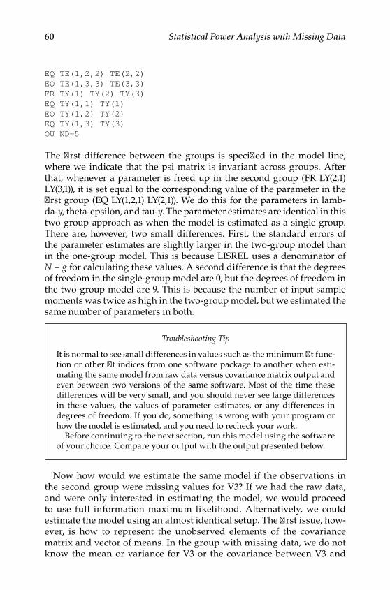
60 Statistical Power Analysis with Missing Data
EQ TE(1,2,2) TE(2,2)EQ TE(1,3,3) TE(3,3)FR TY(1) TY(2) TY(3)EQ TY(1,1) TY(1)EQ TY(1,2) TY(2)EQ TY(1,3) TY(3)OU ND=5
The first difference between the groups is specified in the model line, where we indicate that the psi matrix is invariant across groups. After that, whenever a parameter is freed up in the second group (FR LY(2,1) LY(3,1)), it is set equal to the corresponding value of the parameter in the first group (EQ LY(1,2,1) LY(2,1)). We do this for the parameters in lamb‑da‑y, theta‑epsilon, and tau‑y. The parameter estimates are identical in this two‑group approach as when the model is estimated as a single group. There are, however, two small differences. First, the standard errors of the parameter estimates are slightly larger in the two‑group model than in the one‑group model. This is because LISREL uses a denominator of N − g for calculating these values. A second difference is that the degrees of freedom in the single‑group model are 0, but the degrees of freedom in the two‑group model are 9. This is because the number of input sample moments was twice as high in the two‑group model, but we estimated the same number of parameters in both.
Now how would we estimate the same model if the observations in the second group were missing values for V3? If we had the raw data, and were only interested in estimating the model, we would proceed to use full information maximum likelihood. Alternatively, we could estimate the model using an almost identical setup. The first issue, how‑ever, is how to represent the unobserved elements of the covariance matrix and vector of means. In the group with missing data, we do not know the mean or variance for V3 or the covariance between V3 and
Troubleshooting Tip
It is normal to see small differences in values such as the minimum fit func‑tion or other fit indices from one software package to another when esti‑mating the same model from raw data versus covariance matrix output and even between two versions of the same software. Most of the time these differences will be very small, and you should never see large differences in these values, the values of parameter estimates, or any differences in degrees of freedom. If you do, something is wrong with your program or how the model is estimated, and you need to recheck your work.
Before continuing to the next section, run this model using the software of your choice. Compare your output with the output presented below.
Y100315.indb 60 7/15/09 2:59:08 PM

Missing Data 61
the other variables in our model. They are not estimable from the data observed for this group. As a result, our input data matrices might look like the following:
S X=
=
1 31 0 1 3
55
.
. .? ? ? ?
.and
In order for LISREL to estimate a multiple‑group model, all groups must have the same order for their data structure. Allison (1987) came up with an easy convention to solve this first problem while ensuring that the input covariance matrix does not become non‑positive definite as a result of our convention. Variances for unobserved variables are fixed to values of 1 (so matrices involving missing data remain invertible), and unobserved covariances and means are fixed to values of 0. So now, our input covariance matrix and mean vector for the second group would be
entered as S =
1 31 0 1 30 0 1
.
. . and X =
550
. Any parameters that
can be estimated in both groups are simply equated as we did above.Here are the simple rules for estimating models with missing data. For
any parameters involving unobserved variables, we do the following three things. First, we fix the corresponding elements of lambda‑y equal to 0 for those variables. This ensures that the model is not affected by our inclusion of the zeroes on the off‑diagonals in our input covariance matrix. Second, we remove the effects of putting a 1 on the diagonal for unobserved variables by fixing the corresponding element of theta‑ep‑silon to 1. Finally, to remove the effects of the zeroes in our input vector of means, we fix the corresponding element of tau‑y to a value of 0.
For this example, our syntax for the first (complete) data group would be identical to the model above. Our syntax for the second (incomplete) data group would look like the following:
DA NI=3 NO=500LAV1 V2 V3CM1.31.0 1.30 0 1ME5 5 0
Y100315.indb 61 7/15/09 2:59:09 PM
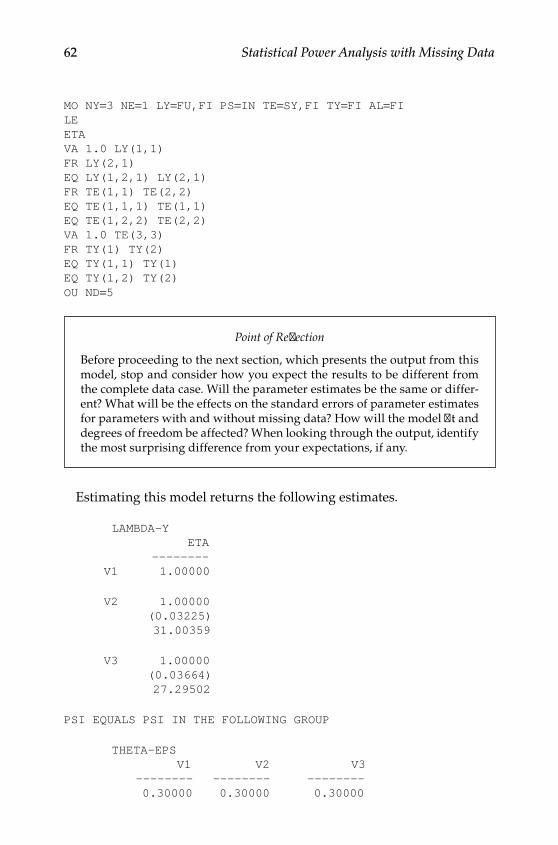
62 Statistical Power Analysis with Missing Data
MO NY=3 NE=1 LY=FU,FI PS=IN TE=SY,FI TY=FI AL=FILEETAVA 1.0 LY(1,1)FR LY(2,1)EQ LY(1,2,1) LY(2,1)FR TE(1,1) TE(2,2)EQ TE(1,1,1) TE(1,1)EQ TE(1,2,2) TE(2,2)VA 1.0 TE(3,3)FR TY(1) TY(2)EQ TY(1,1) TY(1)EQ TY(1,2) TY(2)OU ND=5
Estimating this model returns the following estimates.
LAMBDA-Y ETA -------- V1 1.00000
V2 1.00000 (0.03225) 31.00359
V3 1.00000 (0.03664) 27.29502
PSI EQUALS PSI IN THE FOLLOWING GROUP
THETA-EPS V1 V2 V3 -------- -------- -------- 0.30000 0.30000 0.30000
Point of Reflection
Before proceeding to the next section, which presents the output from this model, stop and consider how you expect the results to be different from the complete data case. Will the parameter estimates be the same or differ‑ent? What will be the effects on the standard errors of parameter estimates for parameters with and without missing data? How will the model fit and degrees of freedom be affected? When looking through the output, identify the most surprising difference from your expectations, if any.
Y100315.indb 62 7/15/09 2:59:09 PM

Missing Data 63
(0.02664) (0.02664) (0.02926) 11.26134 11.26134 10.25411
TAU-Y V1 V2 V3 -------- -------- -------- 5.00000 5.00000 5.00000 (0.03609) (0.03609) (0.04164) 138.53630 138.53630 120.07640
LAMBDA-Y ETA --------V1 1.00000
V2 1.00000 (0.03225) 31.00359
V3 - -
PSI ETA -------- 1.00000 (0.06112) 16.36109
THETA-EPS V1 V2 V3 -------- -------- -------- 0.30000 0.30000 1.00000 (0.02664) (0.02664) 11.26134 11.26134TAU-Y V1 V2 V3 -------- -------- -------- 5.00000 5.00000 - - (0.03609) (0.03609) 138.53630 138.53630Global Goodness of Fit StatisticsDegrees of Freedom = 9Minimum Fit Function Chi-Square = 0.0 (P = 1.00000)Normal Theory Weighted Least Squares Chi-Square = 0.00The Fit is Perfect!
Notice that we obtain the same parameter estimates, although several of our standard errors will differ because they were estimated with differ‑ent portions of the entire sample. There are also other small differences
Y100315.indb 63 7/15/09 2:59:09 PM
64 Statistical Power Analysis with Missing Data
in standard errors even for parameters without any missing data. This is because the parameters of a structural equation model tend to be inter‑related and changes in one part of the system of equations have impli‑cations for other parts of the system. Likewise, the degrees of freedom and overall fit are not adversely affected by our conventions for input of unobserved variables. It takes some time to get comfortable with this approach for estimating structural equation models with incomplete data.
For estimation of a single model, it can also seem like a cumbersome way to proceed compared with FIML analysis of complete data. However, as we will see in subsequent chapters, this approach can be used with only minor modifications to estimate statistical power under an extremely wide range of conditions. In the next chapter, we continue laying the ground‑work for this process by focusing on estimation of statistical power in structural equation modeling with complete data.
Conclusions
In this chapter, we reviewed the main classes of missing data and consid‑ered several examples of each type. We also reviewed many of the most commonly used strategies to address (or ignore) missing data including complete case, available case, and imputation methods. This chapter also illustrated some simple principles that can permit analyses with missing data in a fashion analogous to full information maximum likelihood. It is this approach that forms the foundation of nearly all of the remainder of this book. After delving further into evaluation of statistical power with complete data, we will return to this method and slowly extend it step by step to estimation of statistical power with missing data.
Troubleshooting Tip
Estimating missing data models in this way can be tricky until you start to get the hang of process. Several suggestions can help you ensure that your models are set up correctly. Always start with the complete data group (NG=1). Run this model to ensure that you get the results you were expect‑ing. Then begin adding missing data groups, one at a time, to ensure that you have the input matrices and equality constraints set up correctly. Proceed in this fashion until a group has been added for each of your observed pat‑terns of data. Remember to adjust the number of groups (NG) and number of observations (NO) in each group.
Y100315.indb 64 7/15/09 2:59:09 PM

Missing Data 65
Further Readings
Allison, P. D. (2001). Missing data. Thousand Oaks, CA: Sage.Enders, C. K. (2006). Analyzing structural equation models with missing data. In
G. R. Hancock & R. O. Mueller (Eds.), A second course in structural equation modeling (pp. 313–344). Greenwich, CT: Information Age.
Little, R. J., & Rubin, D. B. (2002). Statistical analysis with missing data (2nd ed.). New York: Wiley.
Schafer, J. L. (1997). Analysis of incomplete multivariate data. Boca Raton, FL: CRC Press.
Exercises
1. Estimate a two‑group model assuming that 50% of the sample is missing on V1 instead of V3.
2. Estimate a three‑group model assuming that 50% of the sample has complete data, 25% of the sample is missing on V2, and 25% of the sample is missing on V3.
3. Write the syntax to estimate the model from question 2c from Chapter 2 assuming that 50% missing data are missing both indi‑cators of the second latent variable.
4. Write the syntax to estimate the model from question 2c from Chapter 2 assuming that 25% of cases are missing the indicators of the third latent variable and that 25% of cases are missing the indicators of both the second and third latent variables.
Y100315.indb 65 7/15/09 2:59:09 PM

Y100315.indb 66 7/15/09 2:59:09 PM
67
4Estimating Statistical Power With Complete Data
Statistical Power in Structural Equation Modeling
Structural equation models pose particular challenges for power analy‑ses. A typical model will involve a large number of parameters, poten‑tially including means and intercepts, regression coefficients, variances, and covariances. Within a single model, each parameter may be esti‑mated with a different degree of precision. Adding to this, parameters are typically not independent, and so the power to test one parameter may likely be influenced by the power to test other parameters being estimated in a given model. Several different approaches have been presented in the literature in order to evaluate statistical power with structural equation models, and we focus on four distinct approaches in this chapter.
Beginning in this chapter, we introduce slightly more of the mathemat‑ics behind these methods. Though it is not imperative that you understand every aspect of every equation, the greater the effort you make to under‑stand these equations, the clearer each step (and its rationale) is likely to be. Each time something new is introduced, stop and test out your under‑standing of it. If we present a formula and some values, stop and calculate the value. If your results differ from ours, back up to the last point where you were following along and try it again.
Because we expect that most readers will learn by doing, our examples are all provided in a step‑by‑step fashion to help facilitate this process. One implication of this approach, however, is that information and concepts tend to cumulate rather quickly. Try to ensure that you are comfortable with each new concept before moving too far forward in the material. Finally, try to remember that this kind of learning tends to be iterative, and some‑thing that may not be clear on one pass may suddenly make more sense the next time you encounter it, perhaps in a slightly different context.
Y100315.indb 67 7/15/09 2:59:10 PM
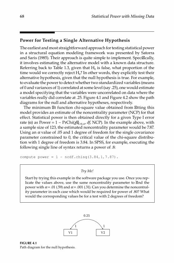
68 Statistical Power with Missing Data
Power for Testing a Single Alternative Hypothesis
The earliest and most straightforward approach for testing statistical power in a structural equation modeling framework was presented by Satorra and Saris (1985). Their approach is quite simple to implement. Specifically, it involves estimating the alternative model with a known data structure. Referring back to Table 1.3, given that H0 is false, what proportion of the time would we correctly reject H0? In other words, they explicitly test their alternative hypothesis, given that the null hypothesis is true. For example, to evaluate the power to detect whether two standardized variables (means of 0 and variances of 1) correlated at some level (say .25), one would estimate a model specifying that the variables were uncorrelated on data where the variables really did correlate at .25. Figure 4.1 and Figure 4.2 show the path diagrams for the null and alternative hypotheses, respectively.
The minimum fit function chi‑square value obtained from fitting this model provides an estimate of the noncentrality parameter (NCP) for that effect. Statistical power is then obtained directly for a given Type I error rate (α) as Power = 1 − PrChi(c²Crit,a, df, NCP). In the example above, with a sample size of 123, the estimated noncentrality parameter would be 7.87. Using an a value of .05 and 1 degree of freedom for the single covariance parameter constrained to 0, the critical value of the chi‑square distribu‑tion with 1 degree of freedom is 3.84. In SPSS, for example, executing the following single line of syntax returns a power of .8:
compute power = 1 - ncdf.chisq(3.84,1,7.87).
Try Me!
Start by trying this example in the software package you use. Once you rep‑licate the values above, use the same noncentrality parameter to find the power with a = .01 (.59) and a = .001 (.31). Can you determine the noncentral‑ity parameter in each case which would be required for power of .80? What would the corresponding values be for a test with 2 degrees of freedom?
1
V1
1
V2
0.25
Figure 4.1Path diagram for the null hypothesis.
Y100315.indb 68 7/15/09 2:59:10 PM
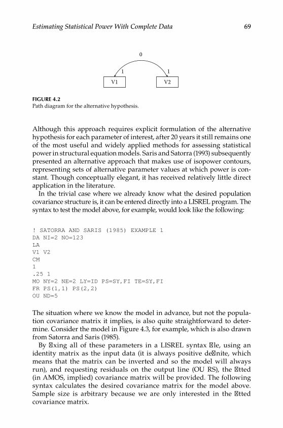
Estimating Statistical Power With Complete Data 69
Although this approach requires explicit formulation of the alternative hypothesis for each parameter of interest, after 20 years it still remains one of the most useful and widely applied methods for assessing statistical power in structural equation models. Saris and Satorra (1993) subsequently presented an alternative approach that makes use of isopower contours, representing sets of alternative parameter values at which power is con‑stant. Though conceptually elegant, it has received relatively little direct application in the literature.
In the trivial case where we already know what the desired population covariance structure is, it can be entered directly into a LISREL program. The syntax to test the model above, for example, would look like the following:
! SATORRA AND SARIS (1985) EXAMPLE 1DA NI=2 NO=123LAV1 V2CM1.25 1MO NY=2 NE=2 LY=ID PS=SY,FI TE=SY,FIFR PS(1,1) PS(2,2)OU ND=5
The situation where we know the model in advance, but not the popula‑tion covariance matrix it implies, is also quite straightforward to deter‑mine. Consider the model in Figure 4.3, for example, which is also drawn from Satorra and Saris (1985).
By fixing all of these parameters in a LISREL syntax file, using an identity matrix as the input data (it is always positive definite, which means that the matrix can be inverted and so the model will always run), and requesting residuals on the output line (OU RS), the fitted (in AMOS, implied) covariance matrix will be provided. The following syntax calculates the desired covariance matrix for the model above. Sample size is arbitrary because we are only interested in the fitted covariance matrix.
1
V1
1
V2
0
Figure 4.2Path diagram for the alternative hypothesis.
Y100315.indb 69 7/15/09 2:59:10 PM
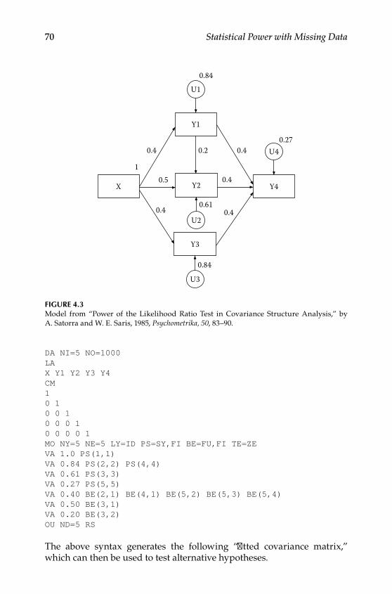
70 Statistical Power with Missing Data
DA NI=5 NO=1000LAX Y1 Y2 Y3 Y4CM10 10 0 10 0 0 10 0 0 0 1MO NY=5 NE=5 LY=ID PS=SY,FI BE=FU,FI TE=ZEVA 1.0 PS(1,1)VA 0.84 PS(2,2) PS(4,4)VA 0.61 PS(3,3)VA 0.27 PS(5,5)VA 0.40 BE(2,1) BE(4,1) BE(5,2) BE(5,3) BE(5,4)VA 0.50 BE(3,1)VA 0.20 BE(3,2)OU ND=5 RS
The above syntax generates the following “fitted covariance matrix,” which can then be used to test alternative hypotheses.
1
X
Y1
Y2
Y3
Y40.5
0.4
0.4
0.4
0.4
0.4
0.2
0.84U1
0.61
U2
0.84
U3
0.27U4
Figure 4.3Model from “Power of the Likelihood Ratio Test in Covariance Structure Analysis,” by A. Satorra and W. E. Saris, 1985, Psychometrika, 50, 83–90.
Y100315.indb 70 7/15/09 2:59:11 PM
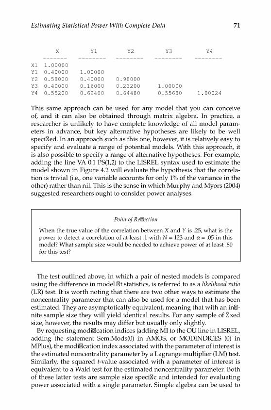
Estimating Statistical Power With Complete Data 71
X Y1 Y2 Y3 Y4 ------- -------- -------- -------- --------X1 1.00000Y1 0.40000 1.00000Y2 0.58000 0.40000 0.98000Y3 0.40000 0.16000 0.23200 1.00000Y4 0.55200 0.62400 0.64480 0.55680 1.00024
This same approach can be used for any model that you can conceive of, and it can also be obtained through matrix algebra. In practice, a researcher is unlikely to have complete knowledge of all model param‑eters in advance, but key alternative hypotheses are likely to be well specified. In an approach such as this one, however, it is relatively easy to specify and evaluate a range of potential models. With this approach, it is also possible to specify a range of alternative hypotheses. For example, adding the line VA 0.1 PS(1,2) to the LISREL syntax used to estimate the model shown in Figure 4.2 will evaluate the hypothesis that the correla‑tion is trivial (i.e., one variable accounts for only 1% of the variance in the other) rather than nil. This is the sense in which Murphy and Myors (2004) suggested researchers ought to consider power analyses.
The test outlined above, in which a pair of nested models is compared using the difference in model fit statistics, is referred to as a likelihood ratio (LR) test. It is worth noting that there are two other ways to estimate the noncentrality parameter that can also be used for a model that has been estimated. They are asymptotically equivalent, meaning that with an infi‑nite sample size they will yield identical results. For any sample of fixed size, however, the results may differ but usually only slightly.
By requesting modification indices (adding MI to the OU line in LISREL, adding the statement Sem.Mods(0) in AMOS, or MODINDICES (0) in MPlus), the modification index associated with the parameter of interest is the estimated noncentrality parameter by a Lagrange multiplier (LM) test. Similarly, the squared t‑value associated with a parameter of interest is equivalent to a Wald test for the estimated noncentrality parameter. Both of these latter tests are sample size specific and intended for evaluating power associated with a single parameter. Simple algebra can be used to
Point of Reflection
When the true value of the correlation between X and Y is .25, what is the power to detect a correlation of at least .1 with N = 123 and a = .05 in this model? What sample size would be needed to achieve power of at least .80 for this test?
Y100315.indb 71 7/15/09 2:59:11 PM
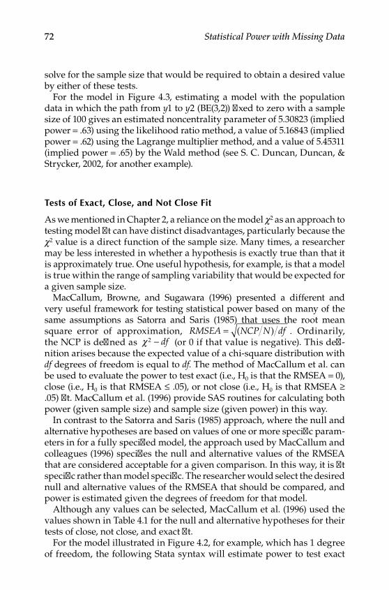
72 Statistical Power with Missing Data
solve for the sample size that would be required to obtain a desired value by either of these tests.
For the model in Figure 4.3, estimating a model with the population data in which the path from y1 to y2 (BE(3,2)) fixed to zero with a sample size of 100 gives an estimated noncentrality parameter of 5.30823 (implied power = .63) using the likelihood ratio method, a value of 5.16843 (implied power = .62) using the Lagrange multiplier method, and a value of 5.45311 (implied power = .65) by the Wald method (see S. C. Duncan, Duncan, & Strycker, 2002, for another example).
Tests of exact, Close, and Not Close Fit
As we mentioned in Chapter 2, a reliance on the model c2 as an approach to testing model fit can have distinct disadvantages, particularly because the c2 value is a direct function of the sample size. Many times, a researcher may be less interested in whether a hypothesis is exactly true than that it is approximately true. One useful hypothesis, for example, is that a model is true within the range of sampling variability that would be expected for a given sample size.
MacCallum, Browne, and Sugawara (1996) presented a different and very useful framework for testing statistical power based on many of the same assumptions as Satorra and Saris (1985) that uses the root mean square error of approximation, RMSEA NCP N df= ( ) . Ordinarily, the NCP is defined as χ 2 − df (or 0 if that value is negative). This defi‑nition arises because the expected value of a chi‑square distribution with df degrees of freedom is equal to df. The method of MacCallum et al. can be used to evaluate the power to test exact (i.e., H0 is that the RMSEA = 0), close (i.e., H0 is that RMSEA ≤ .05), or not close (i.e., H0 is that RMSEA ≥ .05) fit. MacCallum et al. (1996) provide SAS routines for calculating both power (given sample size) and sample size (given power) in this way.
In contrast to the Satorra and Saris (1985) approach, where the null and alternative hypotheses are based on values of one or more specific param‑eters in for a fully specified model, the approach used by MacCallum and colleagues (1996) specifies the null and alternative values of the RMSEA that are considered acceptable for a given comparison. In this way, it is fit specific rather than model specific. The researcher would select the desired null and alternative values of the RMSEA that should be compared, and power is estimated given the degrees of freedom for that model.
Although any values can be selected, MacCallum et al. (1996) used the values shown in Table 4.1 for the null and alternative hypotheses for their tests of close, not close, and exact fit.
For the model illustrated in Figure 4.2, for example, which has 1 degree of freedom, the following Stata syntax will estimate power to test exact
Y100315.indb 72 7/15/09 2:59:11 PM

Estimating Statistical Power With Complete Data 73
fit for our model; close and not close fit can be obtained by running the same syntax with different values from Table 4.1. MacCallum et al. (1996) include similar syntax to run in SAS.
set obs 1generate alpha = 0.05generate rmsea0 = 0.00generate rmseaa = 0.05generate d = 1generate n = 123generate ncp0 = (n - 1)*d*rmsea0*rmsea0generate ncpa = (n - 1)*d*rmseaa*rmseaagenerate cval = invnchi2(d, ncp0, 1 - alpha) /// if rmsea0 < rmseaagenerate power = 1 - nchi2(d, ncpa, cval) /// if rmsea0 < rmseaareplace cval = invnchi2(d, ncp0, alpha) /// if rmsea0 > rmseaareplace power = nchi2(d, ncpa, cval) /// if rmsea0 > rmseaasummarize
Running this syntax for each of these three hypotheses, we find that our power to detect exact, close, and not close fit is .086, .091, and .058, respectively, considerably lower than the power to detect whether the correlation of .25 was different from 0. In order to see why estimated sta‑tistical power is so divergent between the two methods, and also to see the link between the Satorra and Saris (1985) and MacCallum et al. (1996) approaches, we will begin by returning to the output of our LISREL model estimating a zero correlation between the two variables. From that output, the estimated RMSEA was 0.23303. Our test was a comparison of this RMSEA (considerably higher than 0.05) against an alternative of 0.0. Substitution of these values into the Stata syntax above yields an esti‑mated power of .73.
This value is much closer to what we would expect, but it is still low. This is true for two reasons. First, LISREL, unlike other structural equation
Table 4.1
Commonly Used Null and Alternative Values of RMSEA for Tests of Close, Not Close, and Exact FitTest H0 Ha
Close 0.05 0.08Not close 0.05 0.01Exact 0.00 0.05
Y100315.indb 73 7/15/09 2:59:12 PM
74 Statistical Power with Missing Data
modeling software, calculates some aspects of fit, such as the NCP, RMSEA, and c2 for the independence model using a normal theory weighted c2 statis‑tic but uses the minimum fit function value of the c2 for others. Differences between these two types of chi‑square statistics are usually small, but the distinction is something to be aware of. This is another reason we like to test everything and leave as little to chance as possible.
The second, most important reason is that the chi‑square value from our model actually is the estimated NCP and so does not need to be adjusted for the degrees of freedom. So in this case, the RMSEA already reflects the model’s departure from what would be expected in the population.Thus, the corresponding RMSEA NCP N= −( )1 , in this case 0.25404. Substituting this value into our syntax gives us an estimated power of 0.801, just as we would expect. These results highlight two important con‑siderations with regard to statistical power in structural equation model‑ing. First, the power for testing a specific parameter or hypothesis may be quite different from the power to evaluate overall model fit. Second, tests of close and not close fit are likely to be especially useful considerations when evaluating an overall model.
Thus, if you are using the RMSEA from a model estimated with real data, you will probably wish to calculate the RMSEA based on the mini‑mum fit function chi‑square in order to ensure comparability across packages. (In practice, the results obtained from the minimum fit func‑tion chi‑square statistics and the normal theory weighted least squares chi‑square statistic are usually quite comparable.) If you are using the Satorra and Saris (1985) approach, your obtained chi‑square value is the estimated NCP, which can be used to calculate the RMSEA directly, rather than the RMSEA listed in the output.
Troubleshooting Tip
LISREL (and most other packages) can estimate several different kinds of chi‑square values, and the default values may differ across software pack‑ages, models (e.g., model of interest or independence model) or estima‑tion method (e.g., complete data ML or full information ML). In LISREL, for example, you may end up with a minimum fit function value (C1), a normal theory weighted chi‑square (C2), a Satorra‑Bentler chi‑square (C3), or a chi‑square corrected for nonnormality (C4). Adding the option FT to the output line will save additional fit information calculated with each of the chi‑squared values available under a particular estimation method. If your LISREL file is called Test.LS8, the output file will be called Test.FTB. Sadly, this option does not work with multiple‑group or missing data models.
Y100315.indb 74 7/15/09 2:59:12 PM
Estimating Statistical Power With Complete Data 75
Overall, then, one of the primary advantages of this approach is that it is not necessary to completely specify the null and alternative models in order for their framework to be valid. The MacCallum et al. (1996) approach is also consistent with the desire to use non‑nil alternative hypotheses, with its focus on confidence intervals over point estimates, and can be used for any pair of comparisons.
Tests of exact, Close, and Not Close Fit between Two Models
In a more recent paper, MacCallum, Browne, and Cai (2006) extend their approach to comparisons between nested models. When this is the case, the researcher typically has two (or more) models of interest. The models differ by 1 or more degrees of freedom, and the researcher tests the differ‑ence in likelihood ratio chi‑squares between the two models as a function of the expected value for a chi‑square distribution with the difference in degrees of freedom. For this test, the degrees of freedom in each model are not important. Rather, it is the difference in the degrees of freedom that are used for an exact test of difference between the models.
When a researcher is interested in evaluating close fit, however, the results may differ depending on the degrees of freedom in each model. For a given difference in the chi‑square statistic, the power to detect differences will be greater when the models being compared have more degrees of freedom. For a given sample size, comparing two models with 42 and 40 degrees of freedom, respectively, will provide a more powerful test than a comparison of two models with 22 and 20 degrees of freedom.
MacCallum et al. (2006) define the effect size (d, delta) between a pair of nested models, A and B, as the difference between model discrepancy functions. Specifically, δ = −( )* *F FA B where F* is the minimum value of the fit function for each model. In turn, delta can also be expressed in terms of the RMSEA, which MacCallum and colleagues refer to as epsilon (e), and the degrees of freedom for each model. In this case, δ ε ε= −( ).df dfA A B B
2 2 This effect size is standardized in the sense that it is the same regard‑less of sample size. The noncentrality parameter (λ, lambda) is simply the effect size multiplied by the sample size. In other words, λ δ= −( )N 1 .
A simple worked example serves to illustrate their approach. If we have two models with 22 and 20 degrees of freedom that are estimated using a sample size of 200, it is straightforward to estimate our power to detect a difference in RMSEA values of .06 and .04, respectively. We begin by calculating the effect size of the difference in fit between models as δ = × − × = − =( (. ) (. ) ) (. . ) .22 06 20 04 0792 0320 04722 2 . In other words, this is equivalent to testing that the difference between mini‑mum values of the fit functions for the two models is .0472 versus 0. With a sample size of 200, our estimated noncentrality parameter is
Y100315.indb 75 7/15/09 2:59:13 PM
76 Statistical Power with Missing Data
λ = (200 − 1) × 0.0472 or 9.393. The critical value (with a = .05) of a chi‑square distribution with (22 − 20) = 2 degrees of freedom is 5.99. The power to detect these differences is approximately .79. If the mod‑els we are comparing instead had only 12 and 10 degrees of freedom, respectively, the power to detect the same difference would be only .54, but it would be approximately .92 if the models had 32 and 30 degrees of freedom, respectively. Sample Stata syntax to estimate these differ‑ences is presented below.
set obs 1generate n = 200generate alpha = .05generate dfa = 22generate ea = .06generate dfb = 20generate eb = .04generate delta = (dfa*ea*ea - dfb*eb*eb)generate lambda = (n-1)*deltagenerate ddf = dfa - dfbgenerate chicrit = invchi2tail(ddf,alpha)generate power = 1 - nchi2(ddf,lambda,chicrit)
An Alternative Approach to Estimate Statistical Power
In a good recent introductory chapter, Hancock (2006) reviews the above approaches to estimating statistical power, as well as his own extension that incorporates a simplifying assumption about the measurement model. For each latent variable in a model, a single coefficient, which he labels as H, can be defined as a function of the factor loadings for that latent vari‑able. This single value is then used to specify the factor loading (as H ) and residual variance (as 1 − H) for standardized latent variables. The entire structural equation model can then be estimated as a path model.
In other words, going through a little trouble up front to calculate values of H can save considerable work for models with large numbers of indicator
Try Me!
Use the syntax above to replicate the values reported in the text for com‑parisons of 10 vs. 12, 20 vs. 22, and 30 vs. 32 degrees of freedom. Once you have verified our results, find the sample sizes required for power of .80 for each pair of models. If you are comfortable to this point, repeat the exercise for different tests (e.g., close, not close, exact) by using different values of ea and e b.
Y100315.indb 76 7/15/09 2:59:13 PM
Estimating Statistical Power With Complete Data 77
variables. This simplified approach can represent a convenient shorthand method for estimating statistical power. It also allows the researcher to consider how changes in model assumptions can affect statistical power through their effects on H, which ranges from 0 to 1, and reflects the propor‑tion of variance in the latent variable that is accounted for by its indicators.
Consider the example we used to open this chapter, evaluating power to detect whether a correlation of .25 differed significantly from 0. Because it used observed (manifest) variables, this example could not adjust for unreliability of measurement and thus assumed that both variables were measured with perfect reliability. We can use Hancock’s (2006) approach to consider how power would be affected if instead the constructs were each measured with 3 indicators with a reliability of .7, for example.
Calculation of H is quite straightforward:
H i i
k ll
i i
k ll
i
i
i
i
=∑
+ ∑= −
= −
2
2
2
2
1
11
where li is the standardized factor loading for indicator i. Because they are based on standardized values, the factor loading, l is simply the square root of the reliability, in this case, . .7 837= for each indicator. With three indi‑cators, each with a reliability of .7, the numerator of this coefficient wouldbe ( ).
...
.
.73
73
73 7+ + = and the denominator would be ( ) ..
...
.
.1 873
73
73+ + + = The
overall ratio, then, simplifies to 7/8, or .875. This suggests that we shouldfix our factor loadings at a value of .875 or .9354 and our residual vari‑ances at ( . ) . .1 7 3− =
By substituting these values into our model, we can see their effects on the implied covariance matrix. It is easiest to consider in the form of the LISREL syntax to estimate the implied covariance matrix. Our input cova‑riance matrix is an identify matrix, and all model parameters are fixed at their population values. To see the effects of reducing reliability on our implied covariance matrix, we request both the residual matrix and the standardized solution.
! HANCOCK (2006) EXAMPLEDA NI=2 NO=123LAV1 V2CM10 1MO NY=2 NE=2 LY=FU,FI PS=SY,FI TE=SY,FIVA 1.0 PS(1,1) PS(2,2)VA 0.25 PS(1,2)
Y100315.indb 77 7/15/09 2:59:15 PM
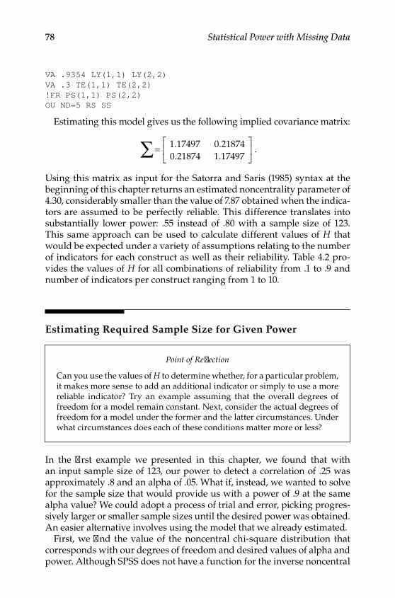
78 Statistical Power with Missing Data
VA .9354 LY(1,1) LY(2,2)VA .3 TE(1,1) TE(2,2)!FR PS(1,1) PS(2,2)OU ND=5 RS SS
Estimating this model gives us the following implied covariance matrix:
=
∑ 1.17497 0.21874
0.21874 1.17497.
Using this matrix as input for the Satorra and Saris (1985) syntax at the beginning of this chapter returns an estimated noncentrality parameter of 4.30, considerably smaller than the value of 7.87 obtained when the indica‑tors are assumed to be perfectly reliable. This difference translates into substantially lower power: .55 instead of .80 with a sample size of 123. This same approach can be used to calculate different values of H that would be expected under a variety of assumptions relating to the number of indicators for each construct as well as their reliability. Table 4.2 pro‑vides the values of H for all combinations of reliability from .1 to .9 and number of indicators per construct ranging from 1 to 10.
Estimating Required Sample Size for Given Power
In the first example we presented in this chapter, we found that with an input sample size of 123, our power to detect a correlation of .25 was approximately .8 and an alpha of .05. What if, instead, we wanted to solve for the sample size that would provide us with a power of .9 at the same alpha value? We could adopt a process of trial and error, picking progres‑sively larger or smaller sample sizes until the desired power was obtained. An easier alternative involves using the model that we already estimated.
First, we find the value of the noncentral chi‑square distribution that corresponds with our degrees of freedom and desired values of alpha and power. Although SPSS does not have a function for the inverse noncentral
Point of Reflection
Can you use the values of H to determine whether, for a particular problem, it makes more sense to add an additional indicator or simply to use a more reliable indicator? Try an example assuming that the overall degrees of freedom for a model remain constant. Next, consider the actual degrees of freedom for a model under the former and the latter circumstances. Under what circumstances does each of these conditions matter more or less?
Y100315.indb 78 7/15/09 2:59:15 PM
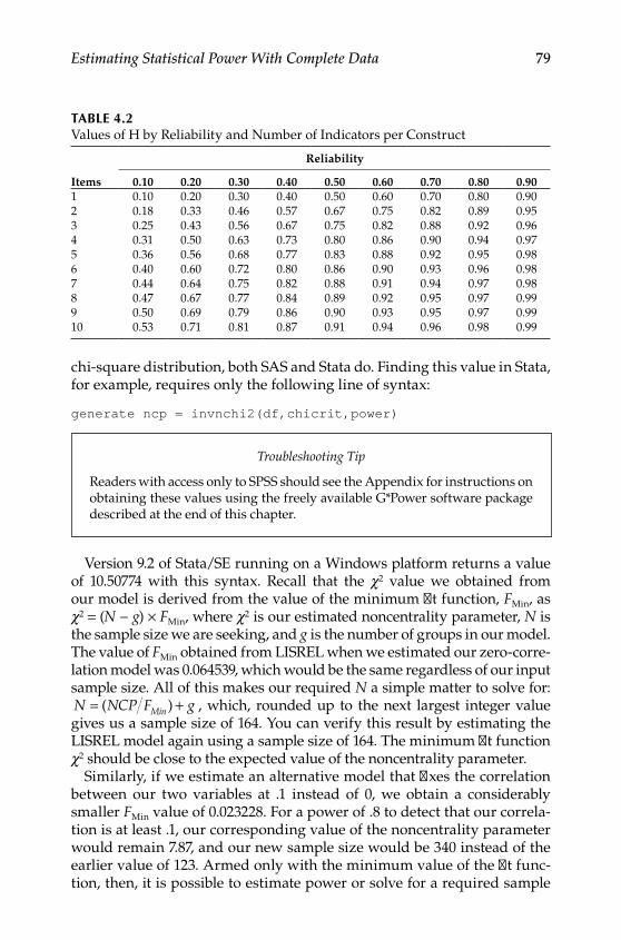
Estimating Statistical Power With Complete Data 79
chi‑square distribution, both SAS and Stata do. Finding this value in Stata, for example, requires only the following line of syntax:
generate ncp = invnchi2(df,chicrit,power)
Version 9.2 of Stata/SE running on a Windows platform returns a value of 10.50774 with this syntax. Recall that the c2 value we obtained from our model is derived from the value of the minimum fit function, FMin, as c2 = (N − g) × FMin, where c2 is our estimated noncentrality parameter, N is the sample size we are seeking, and g is the number of groups in our model. The value of FMin obtained from LISREL when we estimated our zero‑corre‑lation model was 0.064539, which would be the same regardless of our input sample size. All of this makes our required N a simple matter to solve for: N NCP F gMin= +( ) , which, rounded up to the next largest integer value gives us a sample size of 164. You can verify this result by estimating the LISREL model again using a sample size of 164. The minimum fit function c2 should be close to the expected value of the noncentrality parameter.
Similarly, if we estimate an alternative model that fixes the correlation between our two variables at .1 instead of 0, we obtain a considerably smaller FMin value of 0.023228. For a power of .8 to detect that our correla‑tion is at least .1, our corresponding value of the noncentrality parameter would remain 7.87, and our new sample size would be 340 instead of the earlier value of 123. Armed only with the minimum value of the fit func‑tion, then, it is possible to estimate power or solve for a required sample
Troubleshooting Tip
Readers with access only to SPSS should see the Appendix for instructions on obtaining these values using the freely available G*Power software package described at the end of this chapter.
Table 4.2Values of H by Reliability and Number of Indicators per Construct
Reliability
Items 0.10 0.20 0.30 0.40 0.50 0.60 0.70 0.80 0.901 0.10 0.20 0.30 0.40 0.50 0.60 0.70 0.80 0.902 0.18 0.33 0.46 0.57 0.67 0.75 0.82 0.89 0.953 0.25 0.43 0.56 0.67 0.75 0.82 0.88 0.92 0.964 0.31 0.50 0.63 0.73 0.80 0.86 0.90 0.94 0.975 0.36 0.56 0.68 0.77 0.83 0.88 0.92 0.95 0.986 0.40 0.60 0.72 0.80 0.86 0.90 0.93 0.96 0.987 0.44 0.64 0.75 0.82 0.88 0.91 0.94 0.97 0.988 0.47 0.67 0.77 0.84 0.89 0.92 0.95 0.97 0.999 0.50 0.69 0.79 0.86 0.90 0.93 0.95 0.97 0.9910 0.53 0.71 0.81 0.87 0.91 0.94 0.96 0.98 0.99
Y100315.indb 79 7/15/09 2:59:15 PM

80 Statistical Power with Missing Data
size under any desired combinations from estimating a single LISREL model, making this a very flexible and useful approach.
Conclusions
In this chapter, we presented the most commonly used approaches to evaluating statistical power with complete data within a structural equa‑tion modeling framework. Each of the approaches we considered is appli‑cable under a wide variety of circumstances. The Satorra and Saris (1985) approach remains the most widely used approach to statistical power, but the RMSEA‑based approach of MacCallum and colleagues (1996, 2006) has also received widespread use and may be preferable in many contexts because it explicitly permits the researcher to consider the desired null and alternative models. Hancock (2006) presents a useful way to summa‑rize the measurement component of a structural model, which may save considerable time when primary interest lies with associations among latent variables or when the researcher is first deciding on indicators of each latent construct. In subsequent chapters, we will extend each of these approaches to a wide variety of situations involving missing data.
Further Readings
Abraham, W. T., & Russell, D. W. (2008). Statistical power analysis in psychological research. Social and Personality Psychology Compass, 2, 283–301.
Hancock, G. R. (2006). Power analysis in covariance structure modeling. In G. R. Hancock & R. O. Mueller (Eds.), A second course in structural equation modeling (pp. 313–344). Greenwich, CT: Information Age.
MacCallum, R. C., Browne, M. W., & Cai, L. (2006). Testing differences between nested covariance structure models: Power analysis and null hypotheses. Psychological Methods, 11, 19–35.
MacCallum, R. C., Browne, M. W., & Sugawara, H. M. (1996). Power analysis and determination of sample size for covariance structure modeling. Psychological Methods, 1, 130–149.
Exercises
1. Find the sample size needed to obtain power of .8 and .9 for cor‑relations of .1, .3, and .5.
2. Repeat the process above using a = .01.3. Find the sample size required to test whether a correlation of .25
differs from .1 instead of from 0. How would the required sample size change if the indicators had reliability of .8?
Y100315.indb 80 7/15/09 2:59:15 PM

Estimating Statistical Power With Complete Data 81
4. Find the sample size needed to obtain equivalent power values if half of the cases have missing data on one of the variables.
Obtaining and Using G*Power to Calculate Values of Inverse Noncentral Chi‑Square Distribution
Obtaining values of the inverse noncentral chi‑square distribution (quantiles) using G*Power (Faul, Erdfelder, Lang, & Buchner, 2007). G*Power is an extremely useful program for performing a wide variety of power analyses. The G*Power software is free and can be downloaded from http://www.psycho.uni‑duesseldorf.de/abteilun‑gen/aap/gpower3. G*Power can also be used to obtain values of the noncentral chi‑square distribution for readers who do not have access to software that allows for calculation of these values. SPSS, for exam‑ple, does not provide these values.
After installing the G*Power software on your computer, double‑click the program icon. You should see a screen such as the following.
Y100315.indb 81 7/15/09 2:59:16 PM

82 Statistical Power with Missing Data
Obtaining values of the noncentral chi‑square distribution is straight‑forward. Under “Test family” select “c2 tests.” Under “Statistical test” select “Generic c2 test.” Under “Type of power analysis” select “Sensitivity: Compute non‑centrality parameter − given a, and power.” Your screen should now look something like this:
Select the values for a, power, and your degrees of freedom in the “Input Parameters” boxes and then click calculate. In Chapter 4, for example, we found that a noncentrality parameter of 7.87 gave us a power of .80 with a = .05 and 1 degree of freedom. We wanted to iden‑tify the corresponding noncentrality parameter that would provide us with power of .90 under the same circumstances. Enter values of
Y100315.indb 82 7/15/09 2:59:17 PM
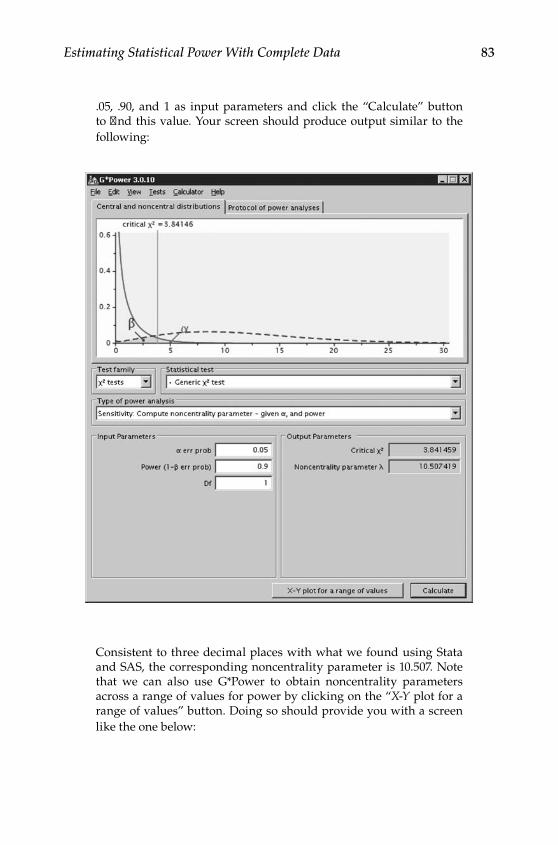
Estimating Statistical Power With Complete Data 83
.05, .90, and 1 as input parameters and click the “Calculate” button to find this value. Your screen should produce output similar to the following:
Consistent to three decimal places with what we found using Stata and SAS, the corresponding noncentrality parameter is 10.507. Note that we can also use G*Power to obtain noncentrality parameters across a range of values for power by clicking on the “X‑Y plot for a range of values” button. Doing so should provide you with a screen like the one below:
Y100315.indb 83 7/15/09 2:59:18 PM

84 Statistical Power with Missing Data
We wish to plot the noncentrality parameter as a function of power and can select a range of values for power. Keeping the default values of .6 to .95, and changing the steps to be .05 instead of .01, we can also click to box to display the values in the plot. When you have done this, click the “Draw plot” button to obtain output like that below:
Y100315.indb 84 7/15/09 2:59:21 PM
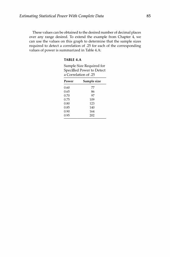
Estimating Statistical Power With Complete Data 85
These values can be obtained to the desired number of decimal places over any range desired. To extend the example from Chapter 4, we can use the values on this graph to determine that the sample sizes required to detect a correlation of .25 for each of the corresponding values of power is summarized in Table 4.A:
Table 4.a
Sample Size Required for Specified Power to Detect a Correlation of .25
Power Sample size
0.60 770.65 860.70 970.75 1090.80 1230.85 1400.90 1640.95 202
Y100315.indb 85 7/15/09 2:59:22 PM

Y100315.indb 86 7/15/09 2:59:22 PM

IISection
Applications
Y100315.indb 87 7/15/09 2:59:22 PM

Y100315.indb 88 7/15/09 2:59:22 PM

89
5Effects of Selection on Means, Variances, and Covariances
Compared with earlier chapters in this book, this chapter contains consid‑erably more equations. In fact, it contains most of the math in this entire book. Partly this is because we have broken everything down step by step. If you are less than comfortable with mathematics and equations in gen‑eral, plan to take your time and to work through each step and try every example and you will do just fine. In most cases, even the most gruesome equations boil down to a small number of actual calculations, many of which you could do by hand.
We will begin with an example. You have a complete data set with 200 observations, and someone tells you to consider a cross‑validation study. On the basis of a coin toss, you create two new data sets (the first called Heads and the second called Tails, say). If a data set were sorted into two groups on a purely random basis such as this one, the data in each group would be expected to be quite comparable. If, on the other hand, the data were sorted on some systematic criterion (suppose you sorted the data set on the basis of one of your key variables and saved your data sets as Best and Worst), the data in each group would necessarily differ in some systematic ways. When the criteria for selection into one group or another are known, it is also pos‑sible to know how the data in each group would be expected to differ from their corresponding population values as a result of this selection.
As another example, we can consider using an aptitude test adminis‑tered on the first day of class to determine which classroom students will be assigned to based on their scores. If all the students who performed best were assigned to classroom A, and those scoring poorest were assigned to classroom B (or maybe better labeled as C, D, or F), we would hardly be surprised if aptitude scores differed between the classrooms at the end of the school year. Selection is the principle that underlies the differ‑ence between data that are missing completely at random (MCAR; there is no selection on anything measured or unmeasured), missing at random (MAR; there is no selection on anything unmeasured), or missing not at random (MNAR; there is selection on something unmeasured). As such, the effects of selection on means and covariances are absolutely essential, and we devote this entire chapter to this issue.
Y100315.indb 89 7/15/09 2:59:22 PM

90 Statistical Power Analysis with Missing Data
In this first application we begin by examining the role of selection or classification into groups (i.e., sorting the data in a systematic fashion) and its effects on the means and covariance matrices for the groups. The purpose of this application is to illustrate how we can go from a known covariance matrix and mean vector to calculating the same quantities in selected subsamples so we can start thinking about data that are MAR.
Defining the Population Model
Let us continue with a similar example from an educational context. An aptitude test is administered to students in two schools at the beginning of the academic year (y1). Within the first school (School A), students are randomized, say on the basis of a coin toss, to an intervention or con‑trol condition and posttest aptitude scores (y2) are again assessed. Within the second school (School B), however, students’ pretest scores (y1) on the aptitude test are used to determine whether they are selected into the intervention program or not (control) and posttest aptitude scores (y2) are again assessed at the end of the intervention program. On the one hand, planning a study as was done in School B is probably not the smartest decision from a research methods perspective. On the other hand, how‑ever, this is very similar to what is often done as students are streamed in one direction (i.e., based on high aptitude) or another (i.e., based on low aptitude). Likewise, students who are in class on a particular day probably have different characteristics than students who are absent from class on a particular day, and so forth. Selection is everywhere.
For the sake of simplicity, let us assume that, in the population, pretest and posttest scores on the aptitude test have a mean of 100 and a stan‑dard deviation of 16 and correlate .25 over the time period considered (equivalent to a medium effect size). The first school, where students are randomly sorted into groups on a variable unrelated to the two observed variables, is basically a complete‑data equivalent of the MCAR condition. The second school, where students are systematically sorted into groups on a variable completely related to an observed variable, is akin to a com‑plete‑data equivalent of the MAR condition.
For this example, if we wished to test whether the pretest and posttest scores were uncorrelated, our alternative model would specify that the correlation was zero, consistent with the example we estimated in Chapter 4. Alternatively, if we wished to test whether the means differed, our alter‑native model would specify that they were identical (i.e., did not differ).
Simple LISREL syntax is provided below to go from population param‑eters to the covariance matrix and vector of means implied by the parameters
Y100315.indb 90 7/15/09 2:59:22 PM

Effects of Selection on Means, Variances, and Covariances 91
provided earlier. As mentioned in Chapter 2, the basic y‑side of the LISREL model for a confirmatory factor model consists of three matrices, Λy (LY), which contains the regression coefficients of the observed variables on the latent vari‑ables, Ψ (PS), a matrix of the latent variable residuals, and Θe (TE), a matrix of the observed variable residuals. (Remember that the I B− portion of the full equation introduced in Chapter 2 simply drops out when all values of B are 0.) We will also include latent intercepts, ty (TY), and means, a (AL). The population covariance matrix among the observed variables implied by our model is calculated as Σ Λ ΨΛ Θyy y y= ′ + ε and the expected vector of means is µ τ αy y= + Λ . We estimate a model with all parameters fixed at their popula‑tion values and request the implied moments using the RS option on the output line, as we first did in Chapter 2.
For our example, we use an identity matrix as our input covariance matrix for the simple reason that it is always positive definite, and we arbitrarily set the means at zero, although any values will work. Although sample size should not affect the results, we find the actual results are more accurate in LISREL with a sample size of at least 1000.
DA NI=2 NO=1000LAY1 Y2CM10 1ME0 0MO NY=2 NE=2 LY=FU,FI PS=SY,FI TE=SY,FI TY=FI AL=FIVA 1 LY(1,1) LY(2,2)VA 256 PS(1,1) PS(2,2)VA 64 PS(1,2)VA 100 TY(1) TY(2)OU RS ND=5
The implied covariance matrix and means can be located in the output under the sections “Fitted Covariance Matrix” and “Fitted Means,” respec‑tively, as shown below. The rest of the output can safely be ignored.
Fitted Covariance Matrix Y1 Y2 -------- -------- Y1 256.00000 Y2 64.00000 256.00000 Fitted Means Y1 Y2 -------- -------- 100.00000 100.00000
Y100315.indb 91 7/15/09 2:59:23 PM

92 Statistical Power Analysis with Missing Data
For this simple example, the above step is hardly needed. The implied
covariance matrix and fitted means are given by Σ =
256 6464 256
and
µ =
100100
.
In order to lay foundations necessary for extending this approach to miss‑ing data situations, we first need to consider how selection affects means and covariance matrices. In the first school, because students were randomly assigned to the two groups, we would expect that the covariance matrix and means would be identical (plus or minus sampling variability) between the intervention and control groups. After all, group composition was decided only by a coin toss, a variable unrelated to anything observed or unobserved.
However, in the second school, the covariance matrix and means would necessarily differ between the intervention (selected) and control (unse‑lected) groups. The covariance matrices would differ because their values are calculated within each group (i.e., deviations from the group means, not the grand mean). The means would differ because we selected them that way. Fortunately, the formulas for how the population covariance matrices and means will be deformed by this selection process have been known for a very long time (cf. Pearson, 1903, 1912), and they are straightforward to calcu‑late, which we will do here. For Monte Carlo applications, a researcher could perform the same steps using raw data (Paxton, Curran, Bollen, Kirby, & Chen, 2001), which we will discuss in much greater detail in Chapter 9. What follows next is a simple example of how to use these formulas to calculate the population matrices and means in the subgroups of the two classrooms.
Defining the Selection Process
The first step is to define the method by which cases are selected into each condition. Individual observations can be selected probabilistically based on a weighted combination of their values on one or more observed vari‑ables. We term this linear combination of these weights with the observed variables s. For the first classroom (MCAR case), the weights for both y1 and y2 would be 0 because, by definition, selection does not depend on
Point of Reflection
In order to ensure that you are comfortable thinking in terms of effect sizes and how they are used to generate data according to a specific population model, repeat the syntax above using different correlations and different means to correspond with small (r = .1 or d = .2), medium (r = .3 or d = .5), and large (r = .5, d = .8) effect sizes. Remember that effects can be specified in terms of covariances or means.
Y100315.indb 92 7/15/09 2:59:23 PM
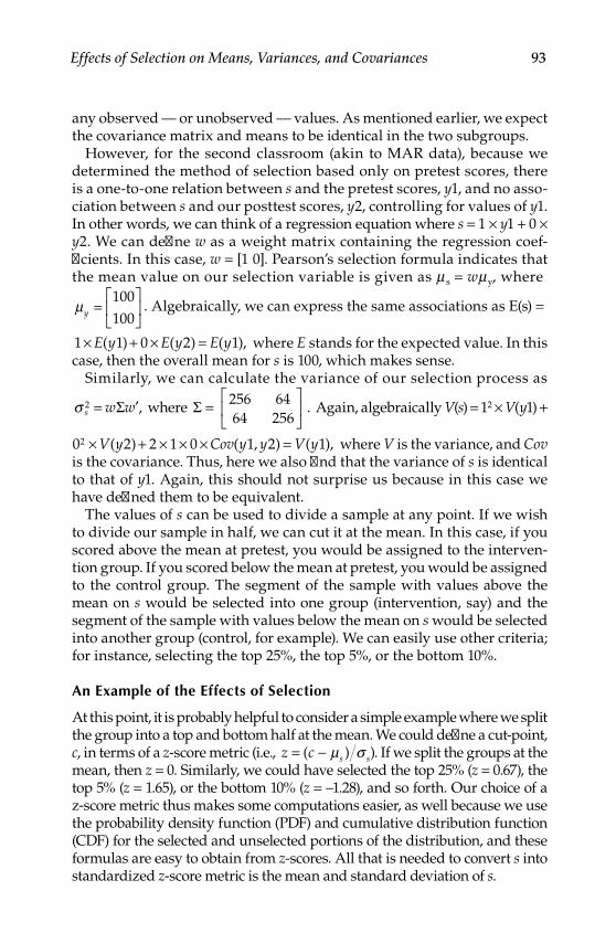
Effects of Selection on Means, Variances, and Covariances 93
any observed — or unobserved — values. As mentioned earlier, we expect the covariance matrix and means to be identical in the two subgroups.
However, for the second classroom (akin to MAR data), because we determined the method of selection based only on pretest scores, there is a one‑to‑one relation between s and the pretest scores, y1, and no asso‑ciation between s and our posttest scores, y2, controlling for values of y1. In other words, we can think of a regression equation where s = 1 × y1 + 0 × y2. We can define w as a weight matrix containing the regression coef‑ficients. In this case, w = [1 0]. Pearson’s selection formula indicates that the mean value on our selection variable is given as m s = wmy, where
µy =
100100
. Algebraically, we can express the same associations as E(s) =
1 1 0 2 1× + × =E y E y E y( ) ( ) ( ), where E stands for the expected value. In this case, then the overall mean for s is 100, which makes sense.
Similarly, we can calculate the variance of our selection process as
σ s w w2 = ′Σ , where Σ =
256 6464 256
. Again, algebraically V(s) = 12 × V(y1) +
0 2 2 1 0 1 2 12 × + × × × =V y Cov y y V y( ) ( , ) ( ), where V is the variance, and Cov is the covariance. Thus, here we also find that the variance of s is identical to that of y1. Again, this should not surprise us because in this case we have defined them to be equivalent.
The values of s can be used to divide a sample at any point. If we wish to divide our sample in half, we can cut it at the mean. In this case, if you scored above the mean at pretest, you would be assigned to the interven‑tion group. If you scored below the mean at pretest, you would be assigned to the control group. The segment of the sample with values above the mean on s would be selected into one group (intervention, say) and the segment of the sample with values below the mean on s would be selected into another group (control, for example). We can easily use other criteria; for instance, selecting the top 25%, the top 5%, or the bottom 10%.
an example of the effects of Selection
At this point, it is probably helpful to consider a simple example where we split the group into a top and bottom half at the mean. We could define a cut‑point, c, in terms of a z‑score metric (i.e., z c s s= −( )µ σ ). If we split the groups at the mean, then z = 0. Similarly, we could have selected the top 25% (z = 0.67), the top 5% (z = 1.65), or the bottom 10% (z = −1.28), and so forth. Our choice of a z‑score metric thus makes some computations easier, as well because we use the probability density function (PDF) and cumulative distribution function (CDF) for the selected and unselected portions of the distribution, and these formulas are easy to obtain from z‑scores. All that is needed to convert s into standardized z‑score metric is the mean and standard deviation of s.
Y100315.indb 93 7/15/09 2:59:24 PM
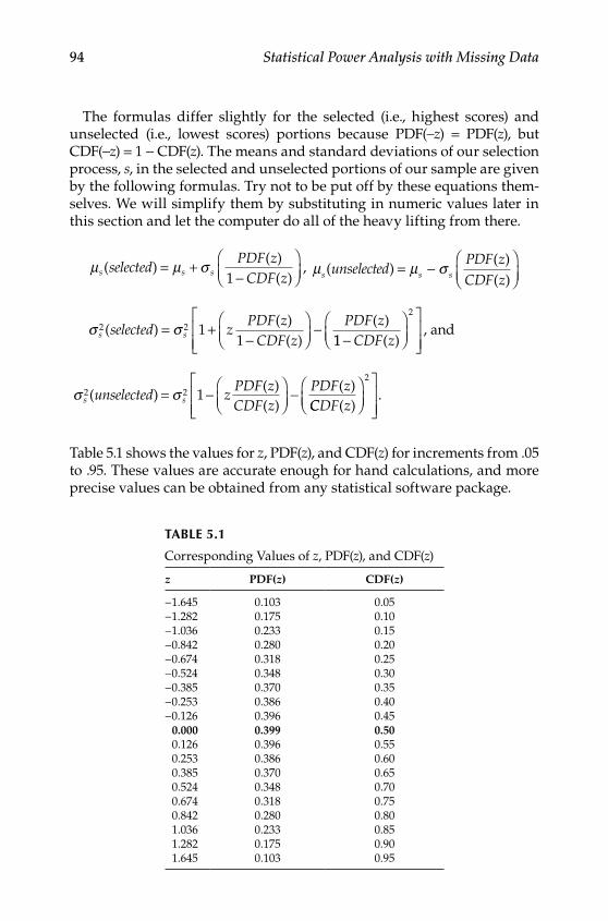
94 Statistical Power Analysis with Missing Data
The formulas differ slightly for the selected (i.e., highest scores) and unselected (i.e., lowest scores) portions because PDF(−z) = PDF(z), but CDF(−z) = 1 − CDF(z). The means and standard deviations of our selection process, s, in the selected and unselected portions of our sample are given by the following formulas. Try not to be put off by these equations them‑selves. We will simplify them by substituting in numeric values later in this section and let the computer do all of the heavy lifting from there.
µ µ σs s sselected
PDF zCDF z
( )( )
( ),= +
−
1
µ µ σs s sunselected
PDF zCDF z
( )( )( )
= −
σ σs sselected zPDF z
CDF zPDF z2 2 1
1( )
( )( )
( )= +−
−11
2
−
CDF z( )
, and
σ σs sunselected zPDF zCDF z
PDF z2 2 1( )( )( )
( )= −
−CCDF z( )
.
2
Table 5.1 shows the values for z, PDF(z), and CDF(z) for increments from .05 to .95. These values are accurate enough for hand calculations, and more precise values can be obtained from any statistical software package.
Table 5.1
Corresponding Values of z, PDF(z), and CDF(z)
z PDF(z) CDF(z)
−1.645 0.103 0.05−1.282 0.175 0.10−1.036 0.233 0.15−0.842 0.280 0.20−0.674 0.318 0.25−0.524 0.348 0.30−0.385 0.370 0.35−0.253 0.386 0.40−0.126 0.396 0.45
0.000 0.399 0.500.126 0.396 0.550.253 0.386 0.600.385 0.370 0.650.524 0.348 0.700.674 0.318 0.750.842 0.280 0.801.036 0.233 0.851.282 0.175 0.901.645 0.103 0.95
Y100315.indb 94 7/15/09 2:59:25 PM
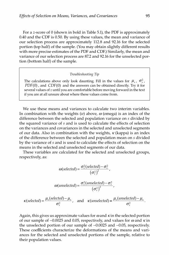
Effects of Selection on Means, Variances, and Covariances 95
For a z‑score of 0 (shown in bold in Table 5.1), the PDF is approximately 0.40 and the CDF is 0.50. By using these values, the mean and variance of our selection process are approximately 112.8 and 92.16 for the selected portion (top half) of the sample. (You may obtain slightly different results with more precise estimates of the PDF and CDF.) Similarly, the mean and variance of our selection process are 87.2 and 92.16 for the unselected por‑tion (bottom half) of the sample.
We use these means and variances to calculate two interim variables. In combination with the weights (w) above, w (omega) is an index of the difference between the selected and population variance on s divided by the squared variance of s and is used to calculate the effects of selection on the variances and covariances in the selected and unselected segments of our data. Also in combination with the weights, k (kappa) is an index of the difference between the selected and population mean on s divided by the variance of s and is used to calculate the effects of selection on the means in the selected and unselected segments of our data.
These variables are calculated for the selected and unselected groups, respectively, as:
ω σ σ
σ( )
( ),selected
selecteds s
s
= −( )
2 2
2 2
ω σ σ
σ( )
( ),unselected
unselecteds s
s
= −( )
2 2
2 2
κ µ µ
σκ( )
( ), ( )selected
selectedunselecteds s
s
= −2
and == −µ µσ
s s
s
unselected( ).
2
Again, this gives us approximate values for w and k in the selected portion of our sample of −0.0025 and 0.05, respectively, and values for w and k in the unselected portion of our sample of −0.0025 and −0.05, respectively. These coefficients characterize the deformations of the means and vari‑ances for the selected and unselected portions of the sample, relative to their population values.
Troubleshooting Tip
The calculations above only look daunting. Fill in the values for µs , σ s2 ,
PDF( )0 , and CDF( )0 and the answers can be obtained directly. Try it for several values of z until you are comfortable before moving forward in the text if you are at all unsure about where these values come from.
Y100315.indb 95 7/15/09 2:59:27 PM
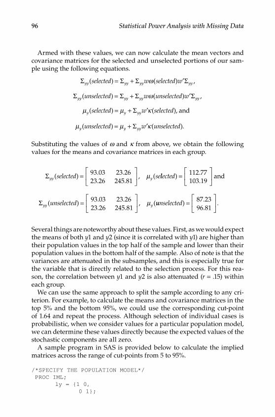
96 Statistical Power Analysis with Missing Data
Armed with these values, we can now calculate the mean vectors and covariance matrices for the selected and unselected portions of our sam‑ple using the following equations.
Σ Σ Σ Σyy yy yy yyselected w selected w( ) ( ) ,= + ′ω
Σ Σ Σ Σyy yy yy yyunselected w unselected w( ) ( ) ,= + ′ω
µ µ κy y yyselected w selected( ) ( ),= + ′Σ and
µ µ κy y yyunselected w unselected( ) ( ).= + ′Σ
Substituting the values of w and k from above, we obtain the following values for the means and covariance matrices in each group.
Σyy yselected se( ) , (=
93.03 23.2623.26 245.81
µ llected) =
112.77103.19
and
Σyy yunselected( ) , (=
93.03 23.2623.26 245.81
µ uunselected) .=
87.2396.81
Several things are noteworthy about these values. First, as we would expect the means of both y1 and y2 (since it is correlated with y1) are higher than their population values in the top half of the sample and lower than their population values in the bottom half of the sample. Also of note is that the variances are attenuated in the subsamples, and this is especially true for the variable that is directly related to the selection process. For this rea‑son, the correlation between y1 and y2 is also attenuated (r = .15) within each group.
We can use the same approach to split the sample according to any cri‑terion. For example, to calculate the means and covariance matrices in the top 5% and the bottom 95%, we could use the corresponding cut‑point of 1.64 and repeat the process. Although selection of individual cases is probabilistic, when we consider values for a particular population model, we can determine these values directly because the expected values of the stochastic components are all zero.
A sample program in SAS is provided below to calculate the implied matrices across the range of cut‑points from 5 to 95%.
/*SPECIFY THE POPULATION MODEL*/ PROC IML; ly = {1 0, 0 1};
Y100315.indb 96 7/15/09 2:59:28 PM

Effects of Selection on Means, Variances, and Covariances 97
ps = {256 64, 64 256}; te = {0 0, 0 0}; ty = {100, 100};/*Specify Weight Matrix*/ w = {1 0}; sigma = ly*ps*ly` + te;/*Mean of Selection Variable - Selection on Observed Variables*/ mus = w*ty;/*Variance of Selection Variable*/ vars = w*sigma*w`;/*Standard Deviation of Selection Variable*/ sds = root(vars);/*This syntax calculated from 5% to 95% cutpoints*/do I = 0.05 to 1 by .05;/*Mean and Variance in Selected Subsample (Greater Than or Equal to Cutpoint)*/d=quantile(‘NORMAL’,I);phis = PDF(‘NORMAL’,trace(d));phiss = CDF(‘NORMAL’,trace(d));xPHIs = I(1)-phiss;/*Mean of Selection Variable (Selected and Unselected Groups*/muss = mus + sds*phis*inv(xPHIs);musu = mus - sds*phis*inv(phiss);/*Variance of Selection Variable (Selected and Unselected Groups*/varss = vars*(1 + (d*phis*inv(xPHIs)) - (phis*phis*inv(xPHIs)*inv(xPHIs)));varsu = vars*(1 - (d*phis*inv(phiss)) - (phis*phis*inv(phiss)*inv(phiss)));/*Omega (Selected and Unselected Groups)*/omegas = inv(vars)*(varss - vars)*inv(vars);omegau = inv(vars)*(varsu - vars)*inv(vars);/*Sigma (Selected and Unselected Groups)*/sigmas = sigma + omegas*(sigma*(w`*w)*sigma);sigmau = sigma + omegau*(sigma*(w`*w)*sigma);/*Kappa (Selected and Unselected Groups)*/ks = inv(vars)*(muss - mus);ku = inv(vars)*(musu - mus);/*Means (Selected and Unselected Groups)*/mues = ks*ps*ly`*w`;mueu = ku*ps*ly`*w`;tys = ty + ly*mues;tyu = ty + ly*mueu;print I sigma ty sigmas tys sigmau tyu;end;quit;
Y100315.indb 97 7/15/09 2:59:28 PM

98 Statistical Power Analysis with Missing Data
Table 5.2 shows the differential effect of splitting the distribution at points from 5 to 95% on each of the five sample moments. The means for the pretest (y1) and posttest score (y2) increase as the proportion of sample increases in the selected group. On the other hand, variances of y1 and y2 both decrease as the proportion of sample increases in the selected group, more for y1 than for y2. Finally, the covariance and correlation between y1 and y2 both decrease substantially as the selected group becomes more highly selected.
Try Me!
Run the syntax for program on the previous page in the software of your choice (see Chapter 5 Appendix) and compare your results with the entries in Table 5.2.
Table 5.2
Effects of Varying Degrees of Selection on Means, Variances, and Covariances
Means Variances Covariance Correlation
Selection Y1 Y2 Y1 Y2 Y1,Y2 Y1,Y2
Top 100% 100.00 100.00 256.00 256.00 64.00 0.25Top 95% 101.74 100.43 207.27 252.95 51.82 0.23Top 90% 103.12 100.78 182.29 251.39 45.57 0.21Top 85% 104.39 101.10 163.96 250.25 40.99 0.20Top 80% 105.60 101.40 149.25 249.33 37.31 0.19Top 75% 106.78 101.69 136.88 248.56 34.22 0.19Top 70% 107.95 101.99 126.16 247.89 31.54 0.18Top 65% 109.12 102.28 116.66 247.29 29.17 0.17Top 60% 110.30 102.58 108.10 246.76 27.02 0.17Top 55% 111.51 102.88 100.27 246.27 25.07 0.16Top 50% 112.77 103.19 93.03 245.81 23.26 0.15Top 45% 114.07 103.52 86.24 245.39 21.56 0.15Top 40% 115.45 103.86 79.83 244.99 19.96 0.14Top 35% 116.93 104.23 73.68 244.61 18.42 0.14Top 30% 118.54 104.64 67.72 244.23 16.93 0.13Top 25% 120.34 105.08 61.86 243.87 15.46 0.13Top 20% 122.40 105.60 55.97 243.50 13.99 0.12Top 15% 124.87 106.22 49.89 243.12 12.47 0.11Top 10% 128.08 107.02 43.30 242.71 10.82 0.11Top 5% 133.00 108.25 35.35 242.21 8.84 0.10
Point of Reflection
All we have done through our selection process is to sort people into dif‑ferent groups. The population parameters remain unchanged. For this rea‑son, if we took the averages across the selected and unselected groups, we would recover our original population parameters.
Y100315.indb 98 7/15/09 2:59:28 PM

Effects of Selection on Means, Variances, and Covariances 99
Selecting Data Into More Than Two Groups
We can also use the same approach to split a population matrix in three parts or more. Let us take the same example of students in a school. After adminis‑tering an aptitude test (y1) in School C, students were split into three groups based on their aptitude test scores: above average, average, and below aver‑age. Aptitude tests were administered again at the end of the school year (y2). The question is how we can determine how this sorting process will affect the means and covariances within each group constructed in this way.
Once again, we assume that in the population pretest and posttest scores on the aptitude test have a mean of 100 and a standard deviation of 16 and correlate .25 over the time period considered (equivalent to a medium effect size). We already know how to get the covariance matrix for the top 33% of the sample (selected = 33%; unselected = 67%), as well as the bottom 33% of the sample (selected = 67%; unselected = 33%). In order to get the covariance matrix for the middle 33% of the sample simple modifications need to be made to the previous program.
In order to do this we must once again define the cut‑points in order to split the classroom into three groups. For the purposes of getting the middle por‑tion of the sample, we will need to define two cut‑points, c1 and c2, in terms of a z‑score metric (i.e., z c s s= −( )µ σ ). Based on the above example, if we split the groups at 33% and 67%, then z1 = −0.44 and z2 = 0.44. The means and stan‑dard deviations of our selection process, s, in the middle portion or selected portion of our sample can now be calculated using the following formulas:
µ µ σs s smiddle
PDF z PDF zCDF z CDF z
( )( ) ( )( ) ( )
= − −−
2 12 1
, and
σ σs smiddlez PDF z z PDF z
CDF z2 2 1
2 2 1 1( )
( ) ( )(
= −× − ×
22 12 12) ( )
( ) ( )( )−
−−−CDF z
PDF z PDF zCDF z CDFF z( )1
2
The PDF for a z‑score of −0.44 and 0.44 is approximately 0.36 for both, and the CDF is 0.33 and 0.67 correspondingly. By using these values, the mean and variance of our selection process are approximately 100 and 15.44 for the middle portion of the sample. Once again, in combination with the weights (w) and the derived mean and variance we can now calculate the two interim variables, w and k, using the following equations:
ω σ σ
σ( )
( )( )
,middlemiddles s
s
= −2 2
2 2and
κ µ µ
σ( )
( ).middle
middles s
s
= −2
Y100315.indb 99 7/15/09 2:59:30 PM
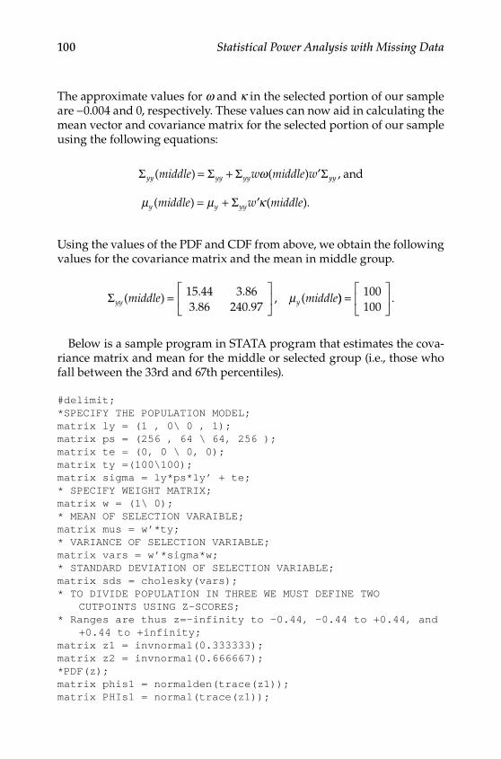
100 Statistical Power Analysis with Missing Data
The approximate values for w and k in the selected portion of our sample are −0.004 and 0, respectively. These values can now aid in calculating the mean vector and covariance matrix for the selected portion of our sample using the following equations:
Σ Σ Σ Σyy yy yy yymiddle w middle w( ) ( ) ,= + ′ω and
µ µ κy y yymiddle w middle( ) ( ).= + ′Σ
Using the values of the PDF and CDF from above, we obtain the following values for the covariance matrix and the mean in middle group.
Σyy ymiddle middle( ) , (=
15.44 3.863.86 240.97
µ )) .=
100100
Below is a sample program in STATA program that estimates the cova‑riance matrix and mean for the middle or selected group (i.e., those who fall between the 33rd and 67th percentiles).
#delimit;*SPECIFY THE POPULATION MODEL;matrix ly = (1 , 0\ 0 , 1);matrix ps = (256 , 64 \ 64, 256 );matrix te = (0, 0 \ 0, 0);matrix ty =(100\100);matrix sigma = ly*ps*ly’ + te;* SPECIFY WEIGHT MATRIX;matrix w = (1\ 0);* MEAN OF SELECTION VARAIBLE;matrix mus = w’*ty;* VARIANCE OF SELECTION VARIABLE;matrix vars = w’*sigma*w;* STANDARD DEVIATION OF SELECTION VARIABLE;matrix sds = cholesky(vars);* TO DIVIDE POPULATION IN THREE WE MUST DEFINE TWO CUTPOINTS USING Z-SCORES;* Ranges are thus z=-infinity to -0.44, -0.44 to +0.44, and +0.44 to +infinity;matrix z1 = invnormal(0.333333);matrix z2 = invnormal(0.666667);*PDF(z);matrix phis1 = normalden(trace(z1));matrix PHIs1 = normal(trace(z1));
Y100315.indb 100 7/15/09 2:59:30 PM

Effects of Selection on Means, Variances, and Covariances 101
*CDF(z);matrix phis2 = normalden(trace(z2));matrix PHIs2 = normal(trace(z2));*MEAN OF SELECTION VARIABLE IN MIDDLE PORTION OF SAMPLE;matrix mm = mus - sds*(phis2-phis1)*inv(PHIs2-PHIs1);*VARIANCE OF SELECTION VARIABLE IN MIDDLE PORTION OF SAMPLE;matrix varsm = vars*(1 - ((z2*phis2-z1*phis1)*inv(PHIs2-PHIs1)) - (phis2-phis1)*(phis2-phis1)*inv(PHIs2- PHIs1)*inv(PHIs2-PHIs1));*STANDARD DEVIATION OF SELECTION VARIABLE IN SELECTED PORTION OF SAMPLE;matrix sds3 = cholesky(varsm);* OMEGA (Selected);matrix omegas = inv(vars)*(varsm - vars)*inv(vars);* KAPPA (Selected and Unselected);matrix ks = inv(vars)*(mm - mus);* SIGMA (Selected);matrix sigmas = sigma + omegas*(sigma*(w*w’)*sigma);* MUY (Selected);matrix muys =ty + sigma*w*ks;matrix list sigmas;matrix list muys;
If the weight matrix used to select data into groups involves variables for which there are missing data, or that are not included in the analytic model, then the resulting data will be MNAR. In this way, researchers can test the effects of violating the assumptions that data are ignorably missing on factors such as power and bias in parameter estimates. This is also a potentially useful way to evaluate and compare the effectiveness of different strategies for dealing with situations where data are suspected to be MNAR.
Conclusions
The purpose of this chapter was to illustrate how to go from a known population covariance matrix and mean vector to calculating the same quantities in certain selected segments of the population. We use the approach outlined in this chapter as the foundation for constructing MAR data in the rest of this book. Millsap and Kwok (2004) have exam‑ined the effects of selection in the context of partial measurement invari‑ance. In the following chapter we extend this approach to situations with missing data.
Y100315.indb 101 7/15/09 2:59:30 PM
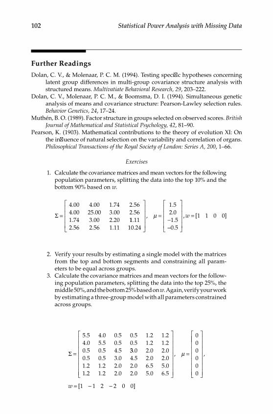
102 Statistical Power Analysis with Missing Data
Further Readings
Dolan, C. V., & Molenaar, P. C. M. (1994). Testing specific hypotheses concerning latent group differences in multi‑group covariance structure analysis with structured means. Multivatiate Behavioral Research, 29, 203–222.
Dolan, C. V., Molenaar, P. C. M., & Boomsma, D. I. (1994). Simultaneous genetic analysis of means and covariance structure: Pearson‑Lawley selection rules. Behavior Genetics, 24, 17–24.
Muthén, B. O. (1989). Factor structure in groups selected on observed scores. British Journal of Mathematical and Statistical Psychology, 42, 81–90.
Pearson, K. (1903). Mathematical contributions to the theory of evolution XI: On the influence of natural selection on the variability and correlation of organs. Philosophical Transactions of the Royal Society of London: Series A, 200, 1–66.
Exercises
1. Calculate the covariance matrices and mean vectors for the following population parameters, splitting the data into the top 10% and the bottom 90% based on w.
Σ =
4 00 4 00 1 74 2 564 00 25 00 3 00 2 561 74 3 00 2 20
. . . .
. . . .
. . . 11 112 56 2 56 1 11 10 24
1 52 01 5.
. . . .
,
.
..
=−
µ
−−
=
0 5
1 1 0 0
.
, [ ]w
2. Verify your results by estimating a single model with the matrices from the top and bottom segments and constraining all param‑eters to be equal across groups.
3. Calculate the covariance matrices and mean vectors for the follow‑ing population parameters, splitting the data into the top 25%, the middle 50%, and the bottom 25% based on w. Again, verify your work by estimating a three‑group model with all parameters constrained across groups.
Σ =
5 5 4 0 0 5 0 5 1 2 1 24 0 5 5 0 5 0 5 1 2 1 20 5 0 5 4 5
. . . . . .
. . . . . .
. . . 33 0 2 0 2 00 5 0 5 3 0 4 5 2 0 2 01 2 1 2 2 0 2 0 6 5 5 01
. . .. . . . . .. . . . . ... . . . . .
,
2 1 2 2 0 2 0 5 0 6 5
000000
=
µ
= − −
,
[ ]w 1 1 2 2 0 0
Y100315.indb 102 7/15/09 2:59:31 PM
103
6Testing Covariances and Mean Differences With Missing Data
This chapter integrates material covered in Chapters 3, 4, and 5 under a single framework. We present a first complete example of how to estimate statisti‑cal power to detect mean differences with incomplete data. We deliberately begin by extending the simple bivariate example first introduced in Chapter 4 to focus on ignorably missing data that are either nonsystematic (missing completely at random, MCAR) or systematic (missing at random, MAR).
In Chapter 5, we examined the effects of selection on means, variances, and covariances for a hypothetical pretest–posttest design. Suppose that instead of following up on all individuals in a longitudinal study, only individuals meeting a specific criterion were administered posttests. Here, we would then have missing observations on the posttest for a portion of the sample. From Chapter 3, we saw that it is still possible to obtain valid parameter estimates of population values when the data mechanism is ignorable, either MCAR or MAR. We now extend this situation to estimate statistical power when data are ignorably missing.
The approach that we use is designed to be simple enough to implement that it encourages researchers to consider a wide variety of conditions. In this chapter, we compare the complete‑data situation with ones with 50% missing data on one variable under MCAR or MAR conditions. We consider this situation with three effect sizes (small, medium, or large correlations) for two different types of tests (mean difference or zero covariance).
The process of conducting a power analysis with missing data can be broken down into seven steps (Davey & Savla, 2009), each of which we have considered in the earlier chapters. First, we specify the population model (H0) based on theory or previous research. Second, we specify one or more alternative models (HA) for which one would like to assess statistical power. In the third step we generate complete data (either raw data or covariances and means) based on the population model. In the fourth step we select an incomplete data model. This is followed by the fifth step in which we apply the incomplete data model to the known data structure. In the sixth step we estimate the population and the alternative models using the incomplete
Y100315.indb 103 7/15/09 2:59:31 PM
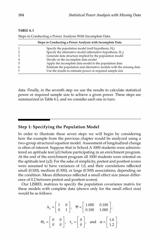
104 Statistical Power Analysis with Missing Data
data. Finally, in the seventh step we use the results to calculate statistical power or required sample size to achieve a given power. These steps are summarized in Table 6.1, and we consider each one in turn.
Step 1: Specifying the Population Model
In order to illustrate these seven steps we will begin by considering how the example from the previous chapter would be analyzed using a two‑group structural equation model. Assessment of longitudinal change is often of interest. Suppose that in School A 1000 students were adminis‑tered an aptitude test (y1) before participating in an enrichment program. At the end of the enrichment program all 1000 students were retested on the aptitude test (y2). For the sake of simplicity, pretest and posttest scores were assumed to have variances of 1.0, and their correlations reflected small (0.100), medium (0.300), or large (0.500) associations, depending on the condition. Mean differences reflected a small effect size (mean differ‑ence of 0.2 between pretest and posttest scores).
Our LISREL matrices to specify the population covariance matrix for these models with complete data (shown only for the small effect size) would be as follows.
Λ Ψy =
=
1 00 1
1 000 0 1000 100 1 000
, . .. .
,
Θε τ α=
=
=
0 00 0
00
1 01 2
, , ..
.y and
Table 6.1
Steps in Conducting a Power Analysis With Incomplete Data
Steps in Conducting a Power Analysis with Incomplete Data
1 Specify the population model (null hypothesis, H0)2 Specify the alternative model (alternative hypothesis, HA)3 Generate data structure implied by the population model4 Decide on the incomplete data model5 Apply the incomplete data model to the population data6 Estimate the population and alternative models with the missing data7 Use the results to estimate power or required sample size
Y100315.indb 104 7/15/09 2:59:31 PM

Testing Covariances and Mean Differences With Missing Data 105
Step 2: Specifying the Alternative Model
For this example, we select two very simple alternative models: (a) that y1 and y2 are uncorrelated, and (b) that the mean of y1 is equal to the mean of y2.
The corresponding matrices would be specified as follows to estimate these alternative models. For both alternative models, the Λy and Θe matri‑ces are the same:
Λ Θy =
=
1 00 1
0 00 0
and ε .
For the first alternative hypothesis,
Ψ =
**
,0
whereas for the second alternative hypothesis
Ψ =
** *
.
For the first alternative hypothesis,
α =
**
,
whereas for the second alternative hypothesis,
α =
aa
,
where use of the same letter for each parameter indicates that they are constrained to the same value.
In LISREL, the syntax to estimate these models would look like the following:
MO NY=2 NE=2 LY=FU,FI PS=SY,FI TE=SY,FI TY=FI AL=FIVA 1.0 LY(1,1) LY(2,2)FR PS(1,1) PS(2,2)FR PS(1,2) ! Remove this line to specify uncorrelated variablesFR AL(1) AL(2)EQ AL(1) AL(2) ! Add this line to specify equal means
Y100315.indb 105 7/15/09 2:59:33 PM
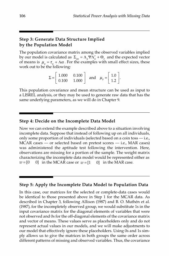
106 Statistical Power Analysis with Missing Data
Step 3: Generate Data Structure Implied by the Population Model
The population covariance matrix among the observed variables implied by our model is calculated as Σ Λ ΨΛ Θyy y y= ′ + ε and the expected vector of means is µ τ αy y= + Λ . For the examples with small effect sizes, these work out to be the following:
Σ =
=
1 000 0 1000 100 1 000
1 01 2
. .
. ...
.and µy
This population covariance and mean structure can be used as input to a LISREL analysis, or they may be used to generate raw data that has the same underlying parameters, as we will do in Chapter 9.
Step 4: Decide on the Incomplete Data Model
Now we can extend the example described above to a situation involving incomplete data. Suppose that instead of following up on all individuals, only some proportion of individuals (selected based on a coin toss — i.e., MCAR cases — or selected based on pretest scores — i.e., MAR cases) was administered the aptitude test following the intervention. Here, observations are missing for a portion of the sample. The weight matrix characterizing the incomplete data model would be represented either asw = [ ]0 0 in the MCAR case or w = [ ]1 0 in the MAR case.
Step 5: Apply the Incomplete Data Model to Population Data
In this case, our matrices for the selected or complete‑data cases would be identical to those presented above in Step 1 for the MCAR data. As described in Chapter 3, following Allison (1987) and B. O. Muthén et al. (1987), for the incompletely observed group, we would substitute 1s in the input covariance matrix for the diagonal elements of variables that were not observed and 0s for the off‑diagonal elements of the covariance matrix and vector of means. These values serve as placeholders only and do not represent actual values in our models, and we will make adjustments to our model that effectively ignore these placeholders. Using 0s and 1s sim‑ply allows us to give the matrices in both groups the same order across different patterns of missing and observed variables. Thus, the covariance
Y100315.indb 106 7/15/09 2:59:34 PM
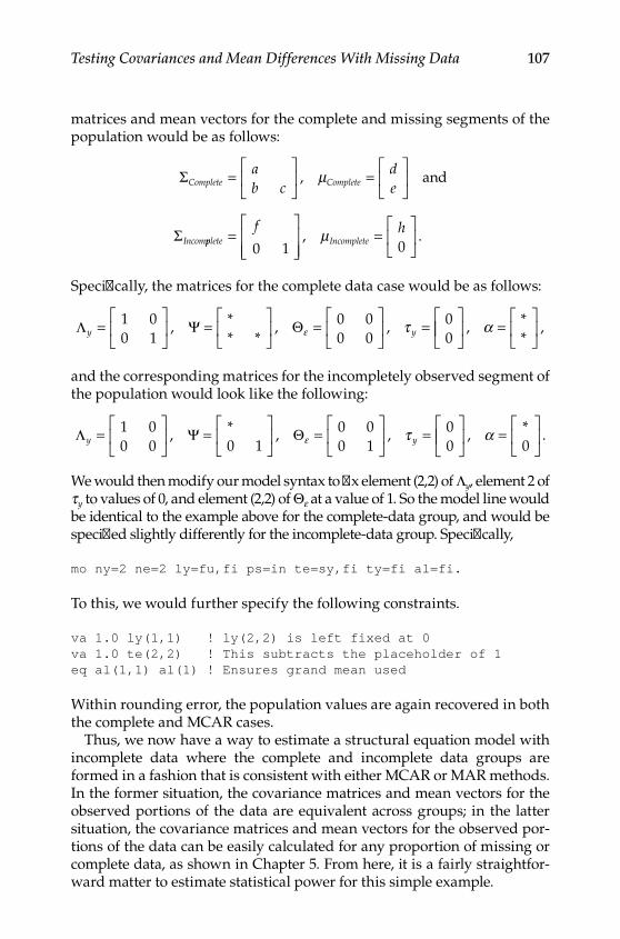
Testing Covariances and Mean Differences With Missing Data 107
matrices and mean vectors for the complete and missing segments of the population would be as follows:
Σ
Σ
Complete Complete
Incom
ab c
de
=
=
, µ and
pplete Incompletef h=
=
0 1 0, .µ
Specifically, the matrices for the complete data case would be as follows:
Λ Ψ Θy y=
=
=
=
1 00 1
0 00 0
00
, ** *
, ,ε τ
=
, *
*,α
and the corresponding matrices for the incompletely observed segment of the population would look like the following:
Λ Ψ Θy y=
=
=
=
1 00 0 0 1
0 00 1
00
, * , ,ε τ
=
, * .α
0
We would then modify our model syntax to fix element (2,2) of Λy, element 2 of ty to values of 0, and element (2,2) of Θe at a value of 1. So the model line would be identical to the example above for the complete‑data group, and would be specified slightly differently for the incomplete‑data group. Specifically,
mo ny=2 ne=2 ly=fu,fi ps=in te=sy,fi ty=fi al=fi.
To this, we would further specify the following constraints.
va 1.0 ly(1,1) ! ly(2,2) is left fixed at 0va 1.0 te(2,2) ! This subtracts the placeholder of 1eq al(1,1) al(1) ! Ensures grand mean used
Within rounding error, the population values are again recovered in both the complete and MCAR cases.
Thus, we now have a way to estimate a structural equation model with incomplete data where the complete and incomplete data groups are formed in a fashion that is consistent with either MCAR or MAR methods. In the former situation, the covariance matrices and mean vectors for the observed portions of the data are equivalent across groups; in the latter situation, the covariance matrices and mean vectors for the observed por‑tions of the data can be easily calculated for any proportion of missing or complete data, as shown in Chapter 5. From here, it is a fairly straightfor‑ward matter to estimate statistical power for this simple example.
Y100315.indb 107 7/15/09 2:59:34 PM

108 Statistical Power Analysis with Missing Data
For this example, we have three different missing data conditions: (a) complete data at pretest and posttest, (b) complete data at pretest and 50% MCAR data at posttest, and (c) complete data at pretest and 50% MAR data at posttest. To generate the MAR situation with 50% missing data on y2, we simply split the data at their middle on the selection variable using the following syntax:
* Specify the population model;matrix ly = (1 , 0 \ 0 , 1 );* Replace Correlations with .3 and .5 for Moderate & Large Effect Sizes;matrix ps = (1.000 , 0.100 \ 0.100 , 1.000 );matrix te = (0 , 0 \ 0 , 0 );matrix ty = (1.0 \ 1.2 );matrix sigma = ly*ps*ly’ + te;* Specify weight matrix;matrix w = (1 \ 0); * Pr(Missing) = f(y1);* Mean of Selection Variable;matrix mus = w’*ty;* Variance of Selection Variable;matrix vars = w’*sigma*w;* Standard Deviation of Selection Variable;matrix sds = cholesky(vars);* Mean and variance in selected subpopulation >= cutpoint, c);matrix z = invnorm(.5);matrix phis = normalden(trace(z)); * PDF(z);matrix PHIs = normal(trace(z)); * CDF(z) and CDF(-z);matrix xPHIs = I(1) - PHIs; * 1 - CDF(z), ie CDF(-z);* Mean of Selection Variable (Selected and Unselected Subpopulations);matrix muss = mus + sds*phis*inv(xPHIs);matrix musu = mus - sds*phis*inv(PHIs);* Variance of Selection Variable (Selected and Unselected Subpopulations);matrix varss = vars*(1 + (z*phis*inv(xPHIs)) - (phis*phis* in v(xPHIs)*inv(xPHIs)));matrix varsu = vars*(1 - (z*phis*inv(PHIs)) - (phis*phis*inv PHIs)*inv(PHIs)));* Omega (Selected and Unselected);matrix omegas = inv(vars)*(varss - vars)*inv(vars);matrix omegau = inv(vars)*(varsu - vars)*inv(vars);* Sigma (Selected and Unselected);matrix sigmas = sigma + omegas*(sigma*(w*w’)*sigma);matrix sigmau = sigma + omegau*(sigma*(w*w’)*sigma);* Kappa (Selected and Unselected);matrix ks = inv(vars)*(muss - mus);matrix ku = inv(vars)*(musu - mus);
Y100315.indb 108 7/15/09 2:59:34 PM
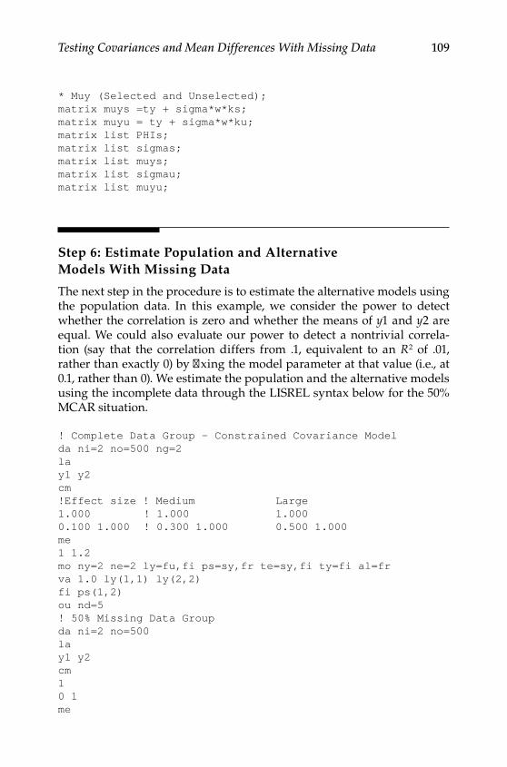
Testing Covariances and Mean Differences With Missing Data 109
* Muy (Selected and Unselected);matrix muys =ty + sigma*w*ks;matrix muyu = ty + sigma*w*ku;matrix list PHIs;matrix list sigmas;matrix list muys;matrix list sigmau;matrix list muyu;
Step 6: Estimate Population and Alternative Models With Missing Data
The next step in the procedure is to estimate the alternative models using the population data. In this example, we consider the power to detect whether the correlation is zero and whether the means of y1 and y2 are equal. We could also evaluate our power to detect a nontrivial correla‑tion (say that the correlation differs from .1, equivalent to an R2 of .01, rather than exactly 0) by fixing the model parameter at that value (i.e., at 0.1, rather than 0). We estimate the population and the alternative models using the incomplete data through the LISREL syntax below for the 50% MCAR situation.
! Complete Data Group - Constrained Covariance Modelda ni=2 no=500 ng=2lay1 y2cm!Effect size ! Medium Large1.000 ! 1.000 1.0000.100 1.000 ! 0.300 1.000 0.500 1.000me1 1.2mo ny=2 ne=2 ly=fu,fi ps=sy,fr te=sy,fi ty=fi al=frva 1.0 ly(1,1) ly(2,2)fi ps(1,2)ou nd=5! 50% Missing Data Groupda ni=2 no=500lay1 y2cm10 1me
Y100315.indb 109 7/15/09 2:59:35 PM

110 Statistical Power Analysis with Missing Data
1 0mo ny=2 ne=2 ly=fu,fi ps=in te=sy,fi ty=fi al=frva 1.0 ly(1,1)va 1.0 te(2,2)eq al(1,1) al(1)fi al(2)ou nd=5
Step 7: Using the Results to Estimate Power or Required Sample Size
Running the syntax directly yields the following values. For the complete data case, we obtain values of the minimum fit function (FMin) of 0.01005 with the covariance fixed at zero and 0 when estimating the model with the covariance freely estimated. For MCAR data with 50% missing, the corresponding values are .00503 and 0, and for MAR data the correspond‑ing values are 1.01414 and 1.01231. The differences between our null and alternative models are thus 0.01005, 0.00503, and 0.00183 for complete, MCAR, and MAR data conditions. These entries are shown in bold type in Table 6.2.
We use the FMin values instead of the χ2 values because most statistical packages calculate χ2 as FMin × (N − g), where N is the sample size, and g is the number of groups. Thus, with complete data, we would get dif‑ferent values of χ2 if we estimated the complete‑data case as one group with a sample size of 1000 or two groups of 500 each, but the value of FMin would be the same in both cases. Because we have to estimate the missing data conditions with one group for each pattern of missing data, only the FMin values are comparable across conditions. In addition, using this value allows us to calculate noncentrality parameters (NCPs) for any desired sample sizes without the need to run any additional models or to
Troubleshooting Tip
One way to make sure that your models are set up correctly is to estimate the H0 model using H0 data and to estimate the HA model using HA data. In this case, your model can use the output to ensure that the population parameters are being correctly recovered. If they are not, there is most likely an error in your syntax. Once you have resolved the issue, substitute the appropriate data back into the syntax.
Y100315.indb 110 7/15/09 2:59:35 PM
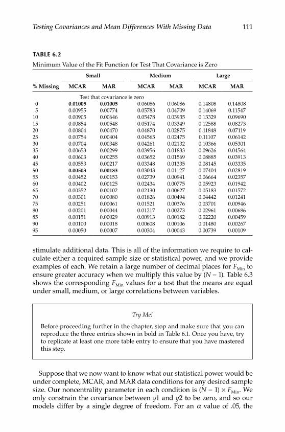
Testing Covariances and Mean Differences With Missing Data 111
stimulate additional data. This is all of the information we require to cal‑culate either a required sample size or statistical power, and we provide examples of each. We retain a large number of decimal places for FMin to ensure greater accuracy when we multiply this value by (N − 1). Table 6.3 shows the corresponding FMin values for a test that the means are equal under small, medium, or large correlations between variables.
Suppose that we now want to know what our statistical power would be under complete, MCAR, and MAR data conditions for any desired sample size. Our noncentrality parameter in each condition is (N − 1) × FMin. We only constrain the covariance between y1 and y2 to be zero, and so our models differ by a single degree of freedom. For an a value of .05, the
Try Me!
Before proceeding further in the chapter, stop and make sure that you can reproduce the three entries shown in bold in Table 6.1. Once you have, try to replicate at least one more table entry to ensure that you have mastered this step.
Table 6.2
Minimum Value of the Fit Function for Test That Covariance is Zero
Small Medium Large
% Missing MCAR MAR MCAR MAR MCAR MAR
Test that covariance is zero 0 0.01005 0.01005 0.06086 0.06086 0.14808 0.14808 5 0.00955 0.00774 0.05783 0.04709 0.14069 0.1154710 0.00905 0.00646 0.05478 0.03935 0.13329 0.0969015 0.00854 0.00548 0.05174 0.03349 0.12588 0.0827320 0.00804 0.00470 0.04870 0.02875 0.11848 0.0711925 0.00754 0.00404 0.04565 0.02475 0.11107 0.0614230 0.00704 0.00348 0.04261 0.02132 0.10366 0.0530135 0.00653 0.00299 0.03956 0.01833 0.09626 0.0456440 0.00603 0.00255 0.03652 0.01569 0.08885 0.0391345 0.00553 0.00217 0.03348 0.01335 0.08145 0.0333550 0.00503 0.00183 0.03043 0.01127 0.07404 0.0281955 0.00452 0.00153 0.02739 0.00941 0.06664 0.0235760 0.00402 0.00125 0.02434 0.00775 0.05923 0.0194265 0.00352 0.00102 0.02130 0.00627 0.05183 0.0157270 0.00301 0.00080 0.01826 0.00494 0.04442 0.0124175 0.00251 0.00061 0.01521 0.00376 0.03701 0.0094680 0.00201 0.00044 0.01217 0.00273 0.02961 0.0068685 0.00151 0.00029 0.00913 0.00182 0.02220 0.0045990 0.00100 0.00018 0.00608 0.00106 0.01480 0.0026795 0.00050 0.00007 0.00304 0.00043 0.00739 0.00109
Y100315.indb 111 7/15/09 2:59:35 PM

112 Statistical Power Analysis with Missing Data
corresponding critical value of the χ2(1) distribution is 3.84. We can now calculate power as ( ) Pr ( , , ),1 1 2− = −β χ αChi df NCPCrit . Below is SAS syn‑tax to calculate statistical power for a given NCP, degrees of freedom, and alpha.
data power;do obs = 1 to 20; FMin0 = 0.01005; *0% missing data; FMin1 = 0.00503; *MCAR with 50% missing; FMin2 = 0.00183; *MAR with 50% missing; n = 50*obs; *n = 250; ncp0 = (n-1)*FMin0; ncp1 = (n-1)*FMin1; ncp2 = (n-1)*FMin2; df = 1; alpha = 0.05; chicrit = quantile(‘chisquare’,1-alpha, 1);; power0 = 1- PROBCHI(chicrit,df,ncp0); power1 = 1- PROBCHI(chicrit,df,ncp1); power2 = 1- PROBCHI(chicrit,df,ncp2);
Table 6.3
Minimum Values of the Fit Function for Test of Equal Means
Small Medium Large
% Missing MCAR MAR MCAR MAR MCAR MAR
Test that means are equal
0 0.02198 0.02198 0.02608 0.02608 0.03130 0.031305 0.02137 0.02144 0.02526 0.02537 0.03022 0.0303710 0.02072 0.02063 0.02440 0.02428 0.02910 0.0289315 0.02004 0.01949 0.02351 0.02277 0.02794 0.0269620 0.01933 0.01804 0.02258 0.02089 0.02674 0.0245325 0.01858 0.01631 0.02162 0.01867 0.02550 0.0217230 0.01780 0.01437 0.02061 0.01626 0.02421 0.0187235 0.01697 0.01232 0.01955 0.01377 0.02288 0.0157040 0.01609 0.01027 0.01845 0.01135 0.02150 0.0128345 0.01517 0.00835 0.01729 0.00913 0.02006 0.0102450 0.01419 0.00660 0.01609 0.00716 0.01858 0.0079855 0.01315 0.00509 0.01482 0.00548 0.01703 0.0060760 0.01204 0.00381 0.01349 0.00408 0.01543 0.0045065 0.01087 0.00277 0.01210 0.00295 0.01376 0.0032470 0.00961 0.00194 0.01063 0.00205 0.01203 0.0022575 0.00828 0.00129 0.00909 0.00136 0.01022 0.0014980 0.00685 0.00080 0.00746 0.00085 0.00834 0.0009385 0.00532 0.00045 0.00574 0.00047 0.00638 0.0005190 0.00367 0.00021 0.00393 0.00023 0.00434 0.0002595 0.00190 0.00006 0.00202 0.00007 0.00222 0.00007
Y100315.indb 112 7/15/09 2:59:35 PM
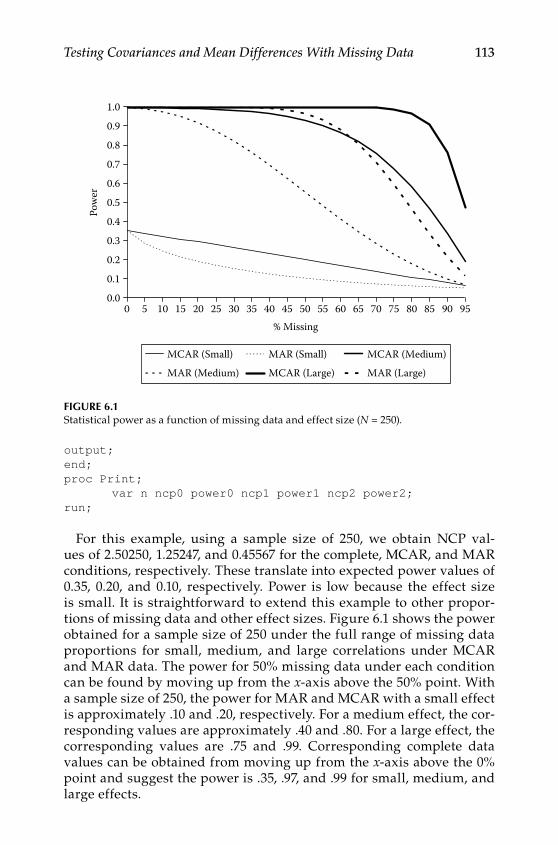
Testing Covariances and Mean Differences With Missing Data 113
output;end;proc Print; var n ncp0 power0 ncp1 power1 ncp2 power2;run;
For this example, using a sample size of 250, we obtain NCP val‑ues of 2.50250, 1.25247, and 0.45567 for the complete, MCAR, and MAR conditions, respectively. These translate into expected power values of 0.35, 0.20, and 0.10, respectively. Power is low because the effect size is small. It is straightforward to extend this example to other propor‑tions of missing data and other effect sizes. Figure 6.1 shows the power obtained for a sample size of 250 under the full range of missing data proportions for small, medium, and large correlations under MCAR and MAR data. The power for 50% missing data under each condition can be found by moving up from the x‑axis above the 50% point. With a sample size of 250, the power for MAR and MCAR with a small effect is approximately .10 and .20, respectively. For a medium effect, the cor‑responding values are approximately .40 and .80. For a large effect, the corresponding values are .75 and .99. Corresponding complete data values can be obtained from moving up from the x‑axis above the 0% point and suggest the power is .35, .97, and .99 for small, medium, and large effects.
0.0
0.1
0.2
0.3
0.4
0.5
0.6
0.7
0.8
0.9
1.0
0 5 10 15 20 25 30 35 40 45 50 55 60 65 70 75 80 85 90 95% Missing
Pow
er
MCAR (Small) MAR (Small) MCAR (Medium)
MAR (Medium) MCAR (Large) MAR (Large)
Figure 6.1Statistical power as a function of missing data and effect size (N = 250).
Y100315.indb 113 7/15/09 2:59:36 PM

114 Statistical Power Analysis with Missing Data
This approach can also be used to determine the sample size required for a specific power level. Suppose that we wanted to obtain the required sample size that would provide an 80% chance of detecting a correlation of .1 under each condition. First we solve for the required noncentrality parameter as NCP InvChi df PowerCrit= ( , , ),χ α
2 . We then calculate the re‑quired sample size as N = NCP/FMin. With 1 degree of freedom, our NCP has to be at least 7.85 to yield a power of .8. This NCP translates into mini‑mum sample sizes of 782, 1562, and 4290 for the complete data, MCAR, and MAR conditions. Again, the corresponding SAS syntax for this calcu‑lation is provided below.
data ncp;df = 1;alpha = 0.05;power = 0.80;chicrit = quantile(‘chisquare’,1-alpha, df);ncp = CINV(power, df, chicrit);fmin0 = 0.01005;fmin1 = 0.00503;fmin2 = 0.00183;n0=ncp/fmin0;n1=ncp/fmin1;n2=ncp/fmin2;output;proc print data=ncp; var df chicrit ncp n0 n1 n2;run;
Figure 6.2 shows the required sample size for power of .8 to test whether the correlation is zero with small, medium, and large correlations as a function of missing data.
Several observations are noteworthy. As can be seen, the required sample size increases much more quickly when the effect size is smaller and also more quickly when data are missing at random than when they are missing completely at random. For this bivariate example, a larger sample size is required to detect a large correlation when data are MAR than is required to detect a medium correlation when data are MCAR once levels of missing data reach approximately 60%. In the bivariate case, it would not generally be wise to deliberately plan a missingness design because once there is more than a trivial amount of missing data, the total sample size to achieve the desired sample size will increase much more rapidly than the complete‑data sample size required to achieve the same statistical power. This is not always the case, however; many times MCAR and MAR designs both provide comparable statisti‑cal power. Finally, it is also worth noting that, faced with incomplete
Y100315.indb 114 7/15/09 2:59:36 PM

Testing Covariances and Mean Differences With Missing Data 115
data, your power will always be greater if you include the partially observed cases in the analysis than if you exclude them, such as through list‑wise deletion.
In Table 6.3 we provide corresponding FMin values for tests that the means are equal with correlations between y1 and y2 of 0.100 (small effect), 0.300 (medium effect), and 0.500 (large effect). In all cases, the mean difference was set at a small effect (means of 1.0 and 1.2 for variables with variances of 1.0), and data are either MCAR or MAR across a range of incomplete data from complete data to 95% missing.
Figure 6.3 shows the power to detect small mean differences when y1 and y2 have a low, moderate, or strong correlation with a total sample size of 250. Note that, in contrast to the test of the correlation itself, the differ‑ence in power between MCAR and MAR conditions is generally greater. We can trace upward from 50% missing data on the x‑axis to read the power values as .47 and .25 for MCAR and MAR data with a small cor‑relation. Corresponding values for a medium correlation are .52 and .27, and they are .58 and .29 for a large correlation. Reading corresponding complete data values from above 0% missing gives powers of .65, .72, and .80 for small, medium, and large correlations.
Figure 6.4 shows the required sample sizes to achieve a power of .8 with 50% missing data for the test of equality of means, respectively, under small, moderate, and strong correlations. As with the test of the correla‑tions themselves, there is not much to recommend a missing data design for this bivariate example. However, power is always greater when all data
0
2000
4000
6000
8000
10000
% Missing
Sam
ple S
ize
MCAR (Small) MAR (Small) MCAR (Medium)MAR (Medium) MCAR (Large) MAR (Large)
0 5 10 15 20 25 30 35 40 45 50 55 60 65 70 75 80 85 90 95
Figure 6.2Sample size required for power of .8 by missing data and effect size.
Y100315.indb 115 7/15/09 2:59:36 PM
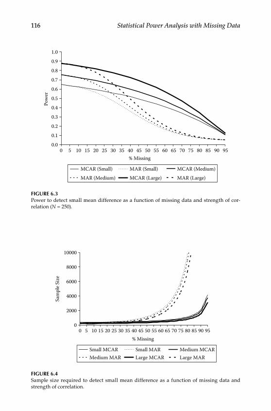
116 Statistical Power Analysis with Missing Data
0
2000
4000
6000
8000
10000
% Missing
Sam
ple S
ize
Small MCAR Small MAR Medium MCARMedium MAR Large MCAR Large MAR
0 5 10 15 20 25 30 35 40 45 50 55 60 65 70 75 80 85 90 95
Figure 6.4Sample size required to detect small mean difference as a function of missing data and strength of correlation.
0.0
0.1
0.2
0.3
0.4
0.5
0.6
0.7
0.8
0.9
1.0
% Missing
Pow
er
MCAR (Small) MAR (Small) MCAR (Medium)MAR (Medium) MCAR (Large) MAR (Large)
0 5 10 15 20 25 30 35 40 45 50 55 60 65 70 75 80 85 90 95
Figure 6.3Power to detect small mean difference as a function of missing data and strength of cor‑relation (N = 250).
Y100315.indb 116 7/15/09 2:59:37 PM

Testing Covariances and Mean Differences With Missing Data 117
are used than when incomplete data are discarded. In most multivariate contexts, this is especially true as we will see in the next chapter.
Conclusions
The purpose of this chapter was to illustrate a simple bivariate example with incomplete data and provide a step‑by‑step guide to calculate statistical power for such a model. In the following chapter we will use a more com‑plex longitudinal design with incomplete data to calculate statistical power.
Further Readings
Dolan, C., van der Sluis, S., & Grasman, R. (2005). A note on normal theory power calculation in SEM with data missing completely at random. Structural Equation Modeling, 12, 245–262.
Graham, J. W. (2009). Missing data analysis: Making it work in the real world. Annual Review of Psychology, 60, 549–576.
Exercises
1. Use the data from Table 6.2 to determine the sample size required to achieve power of .8 (using a = .05) under each condition with 25% missing data.
2. Use the data from Table 6.2 to calculate the power under each con‑dition with 60% missing data and a sample size of 600.
3. Use the data from Table 6.3 to determine the sample size required to achieve power of .9 (using a = .01) under each condition with 50% missing data.
4. Use the data from Table 6.3 to calculate the power under each con‑dition with 15% missing data and a sample size of 300.
Y100315.indb 117 7/15/09 2:59:37 PM

Y100315.indb 118 7/15/09 2:59:37 PM
119
7Testing Group Differences in Longitudinal Change
The previous two applications involved testing covariances and mean dif‑ferences in a test–retest design with data that were ignorably missing. In the present application, we build on these foundations in order to esti‑mate the power to test differences between groups in longitudinal change under conditions involving both randomly (missing completely at random, MCAR) and systematically (missing at random, MAR) missing data.
The Application
Suppose we were interested in testing for gender differences in changes in adolescents’ tolerance of deviant behavior over time. Willett and Sayer (1994) presented an example like this one using a subset of data from the National Youth Survey (see also S. W. Raudenbush & Chan, 1992, for a fuller example that includes application to an accelerated longitudinal design). Data were collected from a sample of 168 boys and girls at ages 11, 12, 13, 14, and 15, and (logged) reported tolerance of deviant behavior was examined, as shown in Table 7.1.
Although this is a quasi‑experimental design (gender cannot, of course, be randomized), the same design could apply equally well to evaluating the effectiveness of an intervention program for changing behavior or performance over time. For example, in order to determine whether an exercise training program increases muscle strength and gait speed or reduces the risk of falling for older adults, a randomized controlled trial design would have a very similar structure, as shown in Table 7.2.
We would begin by assessing strength and functional ability at pretest. Immediately following this, individuals would be randomly assigned to either the treatment (strength training) or the control (passively watching exercise videos) group. Over the course of administering the
Y100315.indb 119 7/15/09 2:59:38 PM
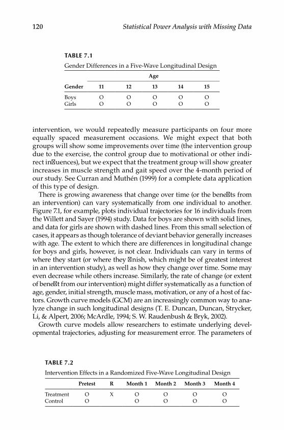
120 Statistical Power Analysis with Missing Data
intervention, we would repeatedly measure participants on four more equally spaced measurement occasions. We might expect that both groups will show some improvements over time (the intervention group due to the exercise, the control group due to motivational or other indi‑rect influences), but we expect that the treatment group will show greater increases in muscle strength and gait speed over the 4‑month period of our study. See Curran and Muthén (1999) for a complete data application of this type of design.
There is growing awareness that change over time (or the benefits from an intervention) can vary systematically from one individual to another. Figure 7.1, for example, plots individual trajectories for 16 individuals from the Willett and Sayer (1994) study. Data for boys are shown with solid lines, and data for girls are shown with dashed lines. From this small selection of cases, it appears as though tolerance of deviant behavior generally increases with age. The extent to which there are differences in longitudinal change for boys and girls, however, is not clear. Individuals can vary in terms of where they start (or where they finish, which might be of greatest interest in an intervention study), as well as how they change over time. Some may even decrease while others increase. Similarly, the rate of change (or extent of benefit from our intervention) might differ systematically as a function of age, gender, initial strength, muscle mass, motivation, or any of a host of fac‑tors. Growth curve models (GCM) are an increasingly common way to ana‑lyze change in such longitudinal designs (T. E. Duncan, Duncan, Strycker, Li, & Alpert, 2006; McArdle, 1994; S. W. Raudenbush & Bryk, 2002).
Growth curve models allow researchers to estimate underlying devel‑opmental trajectories, adjusting for measurement error. The parameters of
Table 7.1
Gender Differences in a Five‑Wave Longitudinal Design
Age
Gender 11 12 13 14 15
Boys O O O O OGirls O O O O O
Table 7.2
Intervention Effects in a Randomized Five‑Wave Longitudinal Design
Pretest R Month 1 Month 2 Month 3 Month 4
Treatment O X O O O OControl O O O O O
Y100315.indb 120 7/15/09 2:59:38 PM
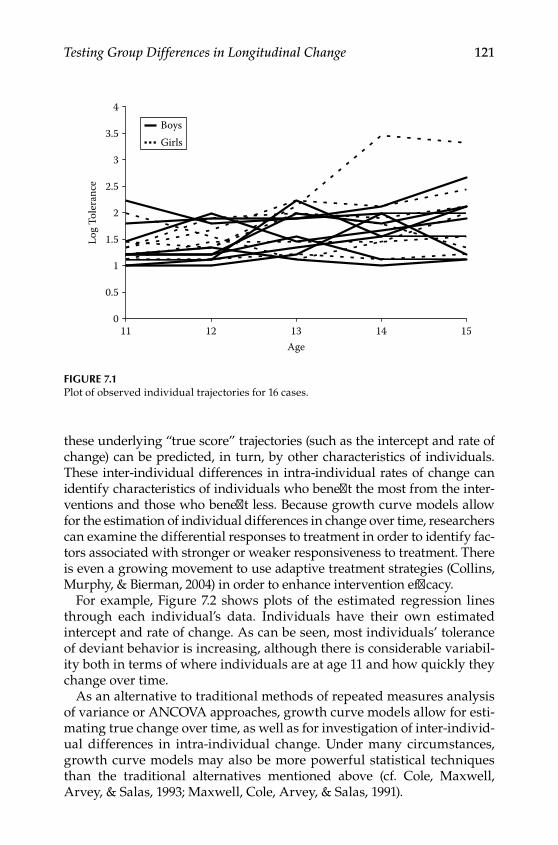
Testing Group Differences in Longitudinal Change 121
these underlying “true score” trajectories (such as the intercept and rate of change) can be predicted, in turn, by other characteristics of individuals. These inter‑individual differences in intra‑individual rates of change can identify characteristics of individuals who benefit the most from the inter‑ventions and those who benefit less. Because growth curve models allow for the estimation of individual differences in change over time, researchers can examine the differential responses to treatment in order to identify fac‑tors associated with stronger or weaker responsiveness to treatment. There is even a growing movement to use adaptive treatment strategies (Collins, Murphy, & Bierman, 2004) in order to enhance intervention efficacy.
For example, Figure 7.2 shows plots of the estimated regression lines through each individual’s data. Individuals have their own estimated intercept and rate of change. As can be seen, most individuals’ tolerance of deviant behavior is increasing, although there is considerable variabil‑ity both in terms of where individuals are at age 11 and how quickly they change over time.
As an alternative to traditional methods of repeated measures analysis of variance or ANCOVA approaches, growth curve models allow for esti‑mating true change over time, as well as for investigation of inter‑individ‑ual differences in intra‑individual change. Under many circumstances, growth curve models may also be more powerful statistical techniques than the traditional alternatives mentioned above (cf. Cole, Maxwell, Arvey, & Salas, 1993; Maxwell, Cole, Arvey, & Salas, 1991).
0
0.5
1
1.5
2
2.5
3
3.5
4
Age11 12 13 14 15
Log
Tole
ranc
e
BoysGirls
Figure 7.1Plot of observed individual trajectories for 16 cases.
Y100315.indb 121 7/15/09 2:59:38 PM
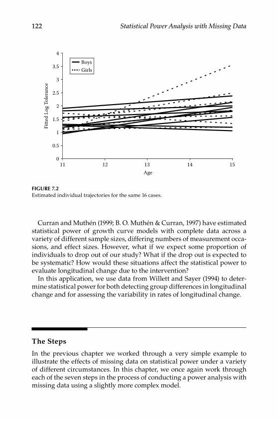
122 Statistical Power Analysis with Missing Data
Curran and Muthén (1999; B. O. Muthén & Curran, 1997) have estimated statistical power of growth curve models with complete data across a variety of different sample sizes, differing numbers of measurement occa‑sions, and effect sizes. However, what if we expect some proportion of individuals to drop out of our study? What if the drop out is expected to be systematic? How would these situations affect the statistical power to evaluate longitudinal change due to the intervention?
In this application, we use data from Willett and Sayer (1994) to deter‑mine statistical power for both detecting group differences in longitudinal change and for assessing the variability in rates of longitudinal change.
The Steps
In the previous chapter we worked through a very simple example to illustrate the effects of missing data on statistical power under a variety of different circumstances. In this chapter, we once again work through each of the seven steps in the process of conducting a power analysis with missing data using a slightly more complex model.
0
0.5
1
1.5
2
2.5
3
3.5
4
Age11 12 13 14 15
Fitte
d Lo
g To
lera
nce
BoysGirls
Figure 7.2Estimated individual trajectories for the same 16 cases.
Y100315.indb 122 7/15/09 2:59:39 PM
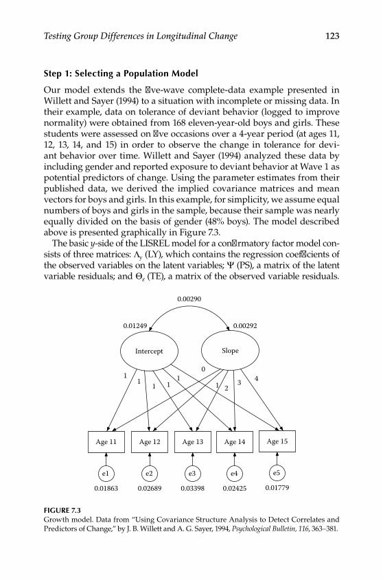
Testing Group Differences in Longitudinal Change 123
Step 1: Selecting a Population Model
Our model extends the five‑wave complete‑data example presented in Willett and Sayer (1994) to a situation with incomplete or missing data. In their example, data on tolerance of deviant behavior (logged to improve normality) were obtained from 168 eleven‑year‑old boys and girls. These students were assessed on five occasions over a 4‑year period (at ages 11, 12, 13, 14, and 15) in order to observe the change in tolerance for devi‑ant behavior over time. Willett and Sayer (1994) analyzed these data by including gender and reported exposure to deviant behavior at Wave 1 as potential predictors of change. Using the parameter estimates from their published data, we derived the implied covariance matrices and mean vectors for boys and girls. In this example, for simplicity, we assume equal numbers of boys and girls in the sample, because their sample was nearly equally divided on the basis of gender (48% boys). The model described above is presented graphically in Figure 7.3.
The basic y‑side of the LISREL model for a confirmatory factor model con‑sists of three matrices: Λy (LY), which contains the regression coefficients of the observed variables on the latent variables; Ψ (PS), a matrix of the latent variable residuals; and Θe (TE), a matrix of the observed variable residuals.
Age 11 Age 12 Age 13 Age 14 Age 15
0.01863
e1
0.02689
e2
0.03398
e3
0.02425
e4
0.01779
e5
0.01249
Intercept
0.00292
Slope
11 1 1
10
1 23 4
0.00290
Figure 7.3Growth model. Data from “Using Covariance Structure Analysis to Detect Correlates and Predictors of Change,” by J. B. Willett and A. G. Sayer, 1994, Psychological Bulletin, 116, 363–381.
Y100315.indb 123 7/15/09 2:59:39 PM
124 Statistical Power Analysis with Missing Data
We will also include latent intercepts, ty (TY), and latent means, a (AL). The estimated population parameters for this model can be specified as follows:
Λ Ψy =
=
1 01 11 21 31 4
, 0.01249 0.002090.000209 0.00292
,
Θε =
0.018630.02689
0.033980.02425
0 0 0 00 0 0 00 0 0 00 0 0 000 0 0 0
000000.01779
and
=
, τ y
for both boys and girls, and
α α=
=0.22062
0.08314for boys and 0.20252
0.065584for girls.
Step 2: Selecting an alternative Model
Having defined our population model, a number of alternative models might be of interest. In this chapter, we focus on two of them. Our pri‑mary interest might be in whether the extent of longitudinal latent change differs between boys and girls. An appropriate alternative hypothesis, then, is that the means do not differ from one another by gender; both groups change, on average, in the same way. The change parameter is rep‑resented by a21 for boys and girls. Our first alternative hypothesis, then, is that a21Boys = a21Girls and will be evaluated with population data where the change parameters differ by (0.08314 − 0.06584), or 0.0173.
A second useful alternative hypothesis that is important in growth curve modeling is whether there is significant variability in how individ‑uals change over time. In other words, is there evidence that individuals change in different ways from one another? Rather than testing whether the variance of the slope term is zero (i.e., everyone changes in an identi‑cal fashion over time as assumed in repeated‑measures analysis of vari‑ance), we compare it with a more realistic alternative that the variance of the latent slope term, represented by element ψ22, can be tested against an alternative hypothesis that it represents a trivial amount of variability, defined here as 50% of its true variability. For the purposes of this example,
Y100315.indb 124 7/15/09 2:59:40 PM
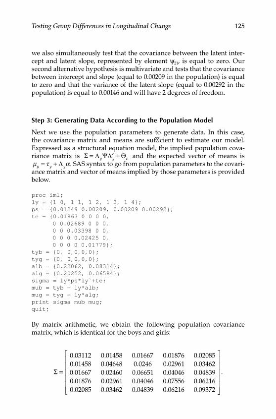
Testing Group Differences in Longitudinal Change 125
we also simultaneously test that the covariance between the latent inter‑cept and latent slope, represented by element ψ21, is equal to zero. Our second alternative hypothesis is multivariate and tests that the covariance between intercept and slope (equal to 0.00209 in the population) is equal to zero and that the variance of the latent slope (equal to 0.00292 in the population) is equal to 0.00146 and will have 2 degrees of freedom.
Step 3: generating Data according to the Population Model
Next we use the population parameters to generate data. In this case, the covariance matrix and means are sufficient to estimate our model. Expressed as a structural equation model, the implied population cova‑riance matrix is Σ Λ ΨΛ Θ= ′ +y y ε and the expected vector of means is µ τ αy y y= + Λ . SAS syntax to go from population parameters to the covari‑ance matrix and vector of means implied by those parameters is provided below.
proc iml;ly = {1 0, 1 1, 1 2, 1 3, 1 4};ps = {0.01249 0.00209, 0.00209 0.00292};te = {0.01863 0 0 0 0, 0 0.02689 0 0 0, 0 0 0.03398 0 0, 0 0 0 0.02425 0, 0 0 0 0 0.01779};tyb = {0, 0,0,0,0};tyg = {0, 0,0,0,0};alb = {0.22062, 0.08314};alg = {0.20252, 0.06584};sigma = ly*ps*ly`+te;mub = tyb + ly*alb;mug = tyg + ly*alg;print sigma mub mug;quit;
By matrix arithmetic, we obtain the following population covariance matrix, which is identical for the boys and girls:
Σ =
0.03112 0.01458 0.01667 0.01876 0.020850.01458 0.044648 0.0246 0.02961 0.034620.01667 0.02460 0.06651 0..04046 0.048390.01876 0.02961 0.04046 0.07556 0.0621160.02085 0.03462 0.04839 0.06216 0.09372
.
Y100315.indb 125 7/15/09 2:59:41 PM
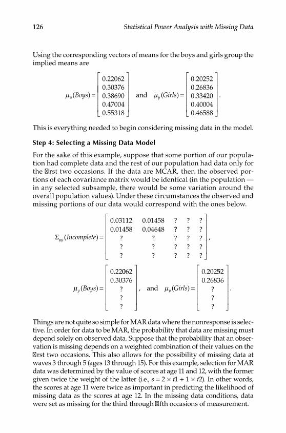
126 Statistical Power Analysis with Missing Data
Using the corresponding vectors of means for the boys and girls group the implied means are
µu Boys( ) =
0.220620.303760.386900.470040.55318
=and
0.202520.268360.334200
µy Girls( )..40004
0.46588
.
This is everything needed to begin considering missing data in the model.
Step 4: Selecting a Missing Data Model
For the sake of this example, suppose that some portion of our popula‑tion had complete data and the rest of our population had data only for the first two occasions. If the data are MCAR, then the observed por‑tions of each covariance matrix would be identical (in the population — in any selected subsample, there would be some variation around the overall population values). Under these circumstances the observed and missing portions of our data would correspond with the ones below.
Σyy Incomplete( )
. . ? ? ?
. .=
0 03112 0 014580 01458 0 04648 ?? ? ?
? ? ? ? ?? ? ? ? ?? ? ? ? ?
,
( )
.
=µy Boys
0 2200620 30376
0 202.
???
, ( )
.
=and µy Girls
5520 26836.
???
.
Things are not quite so simple for MAR data where the nonresponse is selec‑tive. In order for data to be MAR, the probability that data are missing must depend solely on observed data. Suppose that the probability that an obser‑vation is missing depends on a weighted combination of their values on the first two occasions. This also allows for the possibility of missing data at waves 3 through 5 (ages 13 through 15). For this example, selection for MAR data was determined by the value of scores at age 11 and 12, with the former given twice the weight of the latter (i.e., s = 2 × t1 + 1 × t2). In other words, the scores at age 11 were twice as important in predicting the likelihood of missing data as the scores at age 12. In the missing data conditions, data were set as missing for the third through fifth occasions of measurement.
Y100315.indb 126 7/15/09 2:59:41 PM
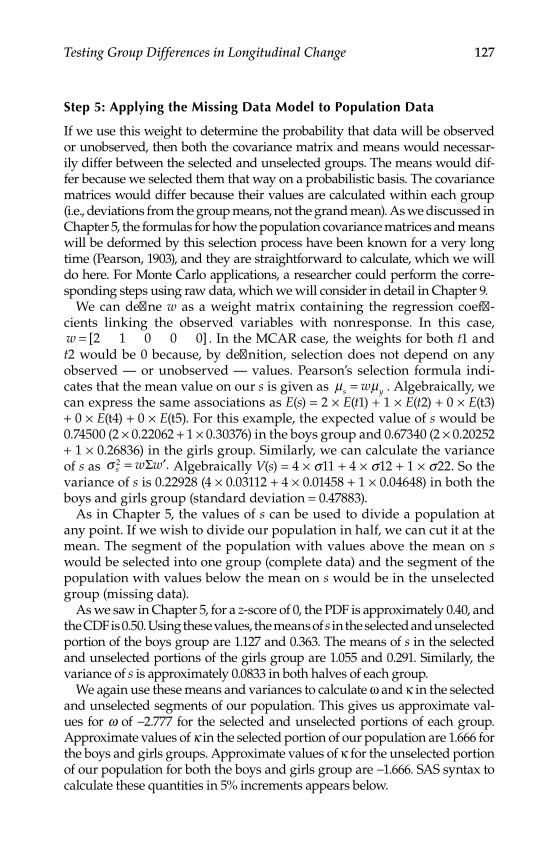
Testing Group Differences in Longitudinal Change 127
Step 5: applying the Missing Data Model to Population Data
If we use this weight to determine the probability that data will be observed or unobserved, then both the covariance matrix and means would necessar‑ily differ between the selected and unselected groups. The means would dif‑fer because we selected them that way on a probabilistic basis. The covariance matrices would differ because their values are calculated within each group (i.e., deviations from the group means, not the grand mean). As we discussed in Chapter 5, the formulas for how the population covariance matrices and means will be deformed by this selection process have been known for a very long time (Pearson, 1903), and they are straightforward to calculate, which we will do here. For Monte Carlo applications, a researcher could perform the corre‑sponding steps using raw data, which we will consider in detail in Chapter 9.
We can define w as a weight matrix containing the regression coeffi‑cients linking the observed variables with nonresponse. In this case, w = [ ]2 1 0 0 0 . In the MCAR case, the weights for both t1 and t2 would be 0 because, by definition, selection does not depend on any observed — or unobserved — values. Pearson’s selection formula indi‑cates that the mean value on our s is given as µ µs yw= . Algebraically, we can express the same associations as E(s) = 2 × E(t1) + 1 × E(t2) + 0 × E(t3) + 0 × E(t4) + 0 × E(t5). For this example, the expected value of s would be 0.74500 (2 × 0.22062 + 1 × 0.30376) in the boys group and 0.67340 (2 × 0.20252 + 1 × 0.26836) in the girls group. Similarly, we can calculate the variance of s as σ s w w2 = ′Σ . Algebraically V(s) = 4 × s11 + 4 × s12 + 1 × s22. So the variance of s is 0.22928 (4 × 0.03112 + 4 × 0.01458 + 1 × 0.04648) in both the boys and girls group (standard deviation = 0.47883).
As in Chapter 5, the values of s can be used to divide a population at any point. If we wish to divide our population in half, we can cut it at the mean. The segment of the population with values above the mean on s would be selected into one group (complete data) and the segment of the population with values below the mean on s would be in the unselected group (missing data).
As we saw in Chapter 5, for a z‑score of 0, the PDF is approximately 0.40, and the CDF is 0.50. Using these values, the means of s in the selected and unselected portion of the boys group are 1.127 and 0.363. The means of s in the selected and unselected portions of the girls group are 1.055 and 0.291. Similarly, the variance of s is approximately 0.0833 in both halves of each group.
We again use these means and variances to calculate ω and κ in the selected and unselected segments of our population. This gives us approximate val‑ues for w of −2.777 for the selected and unselected portions of each group. Approximate values of k in the selected portion of our population are 1.666 for the boys and girls groups. Approximate values of κ for the unselected portion of our population for both the boys and girls group are −1.666. SAS syntax to calculate these quantities in 5% increments appears below.
Y100315.indb 127 7/15/09 2:59:42 PM

128 Statistical Power Analysis with Missing Data
proc iml; ly = {1 0, 1 1, 1 2, 1 3, 1 4}; ps = {0.01249 0.00209, 0.00209 0.00292}; te = {0.01863 0 0 0 0, 0 0.02689 0 0 0, 0 0 0.03398 0 0, 0 0 0 0.02425 0, 0 0 0 0 0.01779}; al = {0.22062, 0.08314}; ty = ly*al; sigma = ly*ps*ly +te; w = {2,1,0,0,0}; mus = w*ty; * Use Boys or Girls Group Means; vars = w*sigma*w`; sds = root(vars); do p = 0.05 to .95 by .05; d=quantile('NORMAL',p); phis = PDF('NORMAL',trace(d)); phiss = CDF('NORMAL',trace(d)); xPHIs = I(1)-phiss; muss = mus + sds*phis*inv(xPHIs); musu = mus - sds*phis*inv(phiss); varss = vars*(1 + (d*phis*inv(xPHIs)) - (phis*phis*inv(xPHIs)*inv(xPHIs))); varsu = vars*(1 - (d*phis*inv(phiss)) - (phis*phis*inv(phiss)*inv(phiss))); omegas = inv(vars)*(varss - vars)*inv(vars); omegau = inv(vars)*(varsu - vars)*inv(vars); sigmas = sigma + omegas*(sigma*(w`*w)*sigma); sigmau = sigma + omegau*(sigma*(w`*w)*sigma); ks = inv(vars)*(muss - mus); ku = inv(vars)*(musu - mus); mues = ks*ps*ly`*w`; mueu = ku*ps*ly`*w`; tys = ty + ly*mues; tyu = ty + ly*mueu; print p, sigma ty sigmas tys sigmau tyu; end;
Step 6: estimating Population and alternative Models With incomplete Data
Using the syntax above, we obtain the following values for the means and covariance matrices for the selected (complete; top half) and unselected (missing; bottom half) portions of our boys and girls groups. Because we divided our population at the mean, the covariance matrix is the same in
Y100315.indb 128 7/15/09 2:59:42 PM
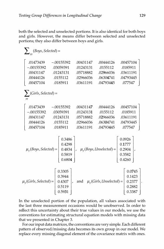
Testing Group Differences in Longitudinal Change 129
both the selected and unselected portions. It is also identical for both boys and girls. However, the means differ between selected and unselected portions; they also differ between boys and girls.
( , )Boys Selectedyy∑ =
−.01473439 .00155392 .00431147 ..00444126 .00457104.00155392 .03059391 .01243131− ..0155112 .0185911
.00431147 .01243131 .05718882 .029966036 .03611191
.00444126 .0155112 .02966036 .063044741 .04793445
.00457104 .0185911 .03611191 .047934445 .077547
( , )Girls Selectedyy
=
−
∑.01473439 .00155392 .004311477 .00444126 .00457104.00155392 .03059391 .0124313− 11 .0155112 .0185911
.00431147 .01243131 .05718882 .022966036 .03611191
.00444126 .0155112 .02966036 .063004741 .04793445
.00457104 .0185911 .03611191 .047934445 .077547
µy Boys Selected( , ) =
0.34860.42980.48340.58190.68044
0.09260.
=, ( , )µy Boys Unselected11777
0.29040.35820.4260
,
µy Girls Selected( , ) =
0.33050.39440.43070.51190.59331
and
0.0
=, ( , )µy Girls Unselected
77450.14230.23770.28820.3387
.
In the unselected portion of the population, all values associated with the last three measurement occasions would be unobserved. In order to reflect this uncertainty about their true values in our models, we use the conventions for estimating structural equation models with missing data that we presented in Chapter 3.
For our input data matrices, the conventions are very simple. Each different pattern of observed/missing data becomes its own group in our model. We replace every missing diagonal element of the covariance matrix with ones.
Y100315.indb 129 7/15/09 2:59:43 PM
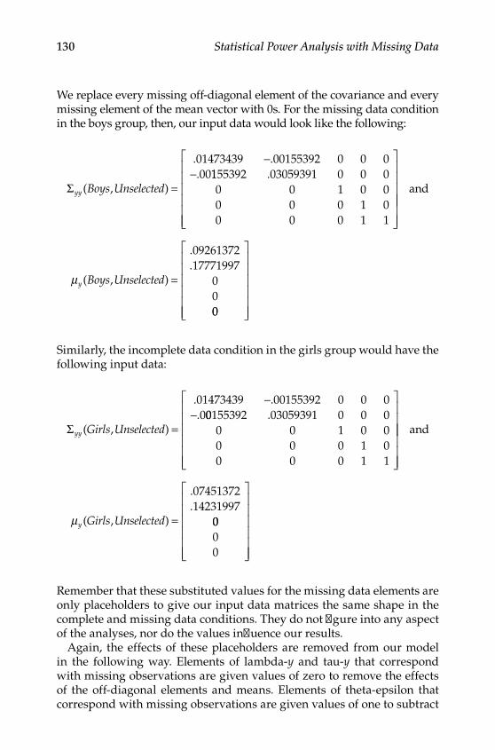
130 Statistical Power Analysis with Missing Data
We replace every missing off‑diagonal element of the covariance and every missing element of the mean vector with 0s. For the missing data condition in the boys group, then, our input data would look like the following:
Σyy Boys Unselected( , ) =
−−.01473439 .00155392.00
0 0 01155392 .03059391 0 0 00 0 1 0 00 0 0 1 00 0 0 1 1
=
and
.09261372
.17771997µy Boys Unselected( , ) 0
000
Similarly, the incomplete data condition in the girls group would have the following input data:
Σyy Girls Unselected( , ) =
−−.01473439 .00155392.0
0 0 000155392 .03059391 0 0 0
0 0 1 0 00 0 0 1 00 0 0 1 1
=
and
.07451372
.14231997µy Girls Unselected( , ) 00
00
Remember that these substituted values for the missing data elements are only placeholders to give our input data matrices the same shape in the complete and missing data conditions. They do not figure into any aspect of the analyses, nor do the values influence our results.
Again, the effects of these placeholders are removed from our model in the following way. Elements of lambda‑y and tau‑y that correspond with missing observations are given values of zero to remove the effects of the off‑diagonal elements and means. Elements of theta‑epsilon that correspond with missing observations are given values of one to subtract
Y100315.indb 130 7/15/09 2:59:43 PM
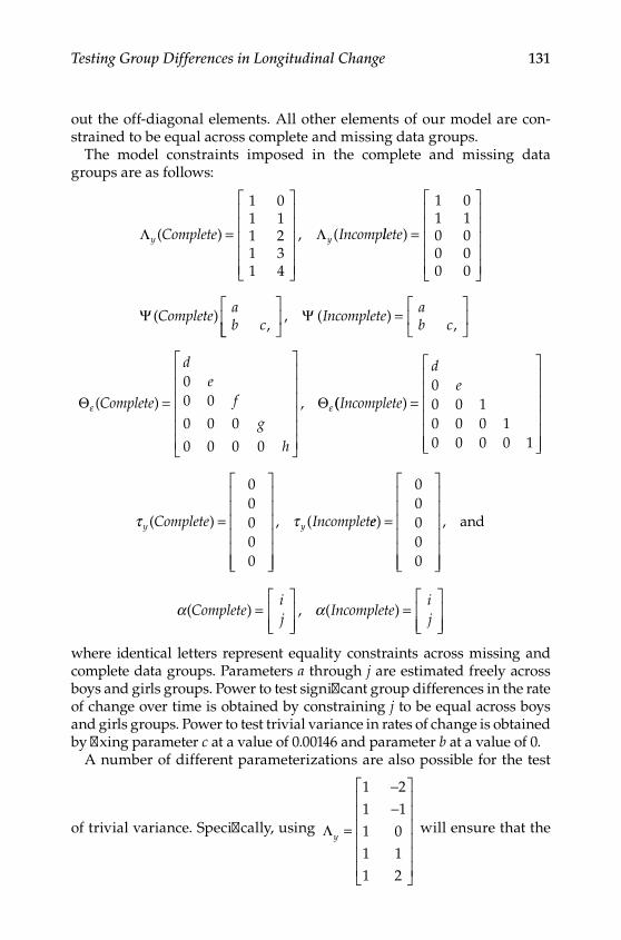
Testing Group Differences in Longitudinal Change 131
out the off‑diagonal elements. All other elements of our model are con‑strained to be equal across complete and missing data groups.
The model constraints imposed in the complete and missing data groups are as follows:
Λ Λy yComplete Incomp( ) , (=
1 01 11 21 31 4
llete
ab c
)
( ),
=
1 01 10 00 00 0
Ψ Complete
=
, ( )
,Ψ Incomplete a
b c
Θ Θε ε( ) ,Complete
de
f
g
h
=
00 0
0 0 0
0 0 0 0
(( )Incomplete
de
=
00 0 10 0 0 10 0 0 0 1
τ τy yComplete Incomplet( ) , (=
00000
ee) ,=
00000
and
α α( ) , ( )Complete
ij
Incompleteij
=
=
where identical letters represent equality constraints across missing and complete data groups. Parameters a through j are estimated freely across boys and girls groups. Power to test significant group differences in the rate of change over time is obtained by constraining j to be equal across boys and girls groups. Power to test trivial variance in rates of change is obtained by fixing parameter c at a value of 0.00146 and parameter b at a value of 0.
A number of different parameterizations are also possible for the test
of trivial variance. Specifically, using Λy =
−−
1 21 11 01 11 2
will ensure that the
Y100315.indb 131 7/15/09 2:59:45 PM
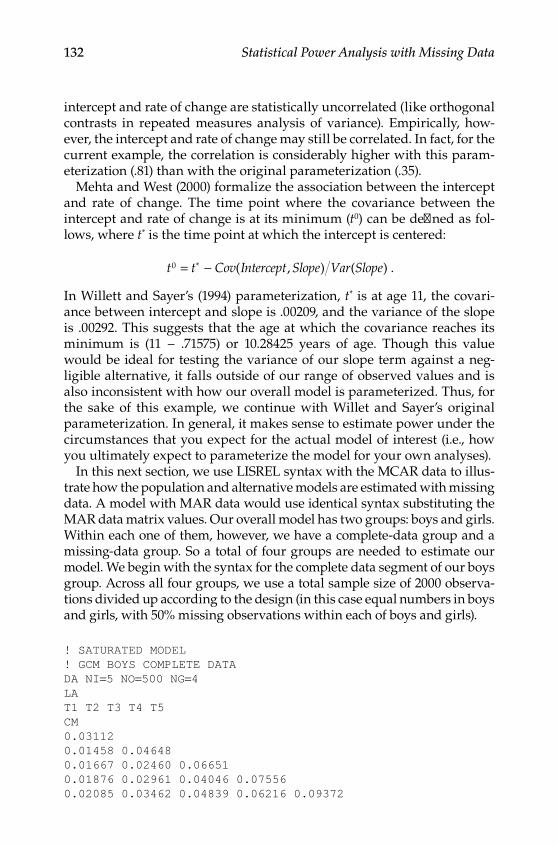
132 Statistical Power Analysis with Missing Data
intercept and rate of change are statistically uncorrelated (like orthogonal contrasts in repeated measures analysis of variance). Empirically, how‑ever, the intercept and rate of change may still be correlated. In fact, for the current example, the correlation is considerably higher with this param‑eterization (.81) than with the original parameterization (.35).
Mehta and West (2000) formalize the association between the intercept and rate of change. The time point where the covariance between the intercept and rate of change is at its minimum (t0) can be defined as fol‑lows, where t* is the time point at which the intercept is centered:
t t Cov Intercept Slope Var Slope0 = −* ( , ) ( ) .
In Willett and Sayer’s (1994) parameterization, t* is at age 11, the covari‑ance between intercept and slope is .00209, and the variance of the slope is .00292. This suggests that the age at which the covariance reaches its minimum is (11 − .71575) or 10.28425 years of age. Though this value would be ideal for testing the variance of our slope term against a neg‑ligible alternative, it falls outside of our range of observed values and is also inconsistent with how our overall model is parameterized. Thus, for the sake of this example, we continue with Willet and Sayer’s original parameterization. In general, it makes sense to estimate power under the circumstances that you expect for the actual model of interest (i.e., how you ultimately expect to parameterize the model for your own analyses).
In this next section, we use LISREL syntax with the MCAR data to illus‑trate how the population and alternative models are estimated with missing data. A model with MAR data would use identical syntax substituting the MAR data matrix values. Our overall model has two groups: boys and girls. Within each one of them, however, we have a complete‑data group and a missing‑data group. So a total of four groups are needed to estimate our model. We begin with the syntax for the complete data segment of our boys group. Across all four groups, we use a total sample size of 2000 observa‑tions divided up according to the design (in this case equal numbers in boys and girls, with 50% missing observations within each of boys and girls).
! SATURATED MODEL! GCM BOYS COMPLETE DATADA NI=5 NO=500 NG=4LAT1 T2 T3 T4 T5CM0.031120.01458 0.046480.01667 0.02460 0.066510.01876 0.02961 0.04046 0.075560.02085 0.03462 0.04839 0.06216 0.09372
Y100315.indb 132 7/15/09 2:59:45 PM
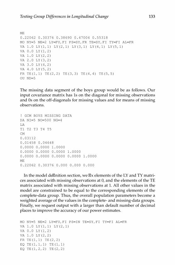
Testing Group Differences in Longitudinal Change 133
ME0.22062 0.30376 0.38690 0.47004 0.55318MO NY=5 NE=2 LY=FU,FI PS=SY,FR TE=SY,FI TY=FI AL=FRVA 1.0 LY(1,1) LY(2,1) LY(3,1) LY(4,1) LY(5,1)VA 0.0 LY(1,2)VA 1.0 LY(2,2)VA 2.0 LY(3,2)VA 3.0 LY(4,2)VA 4.0 LY(5,2)FR TE(1,1) TE(2,2) TE(3,3) TE(4,4) TE(5,5)OU ND=5
The missing data segment of the boys group would be as follows. Our input covariance matrix has 1s on the diagonal for missing observations and 0s on the off‑diagonals for missing values and for means of missing observations.
! GCM BOYS MISSING DATADA NI=5 NO=500 NG=4LAT1 T2 T3 T4 T5CM0.031120.01458 0.046480.0000 0.0000 1.00000.0000 0.0000 0.0000 1.00000.0000 0.0000 0.0000 0.0000 1.0000ME0.22062 0.30376 0.000 0.000 0.000
In the model definition section, we fix elements of the LY and TY matri‑ces associated with missing observations at 0, and the elements of the TE matrix associated with missing observations at 1. All other values in the model are constrained to be equal to the corresponding elements of the complete‑data group. Thus, the overall population parameters become a weighted average of the values in the complete‑ and missing‑data groups. Finally, we request output with a larger than default number of decimal places to improve the accuracy of our power estimates.
MO NY=5 NE=2 LY=FU,FI PS=IN TE=SY,FI TY=FI AL=FRVA 1.0 LY(1,1) LY(2,1)VA 0.0 LY(1,2)VA 1.0 LY(2,2)FR TE(1,1) TE(2,2)EQ TE(1,1,1) TE(1,1)EQ TE(1,2,2) TE(2,2)
Y100315.indb 133 7/15/09 2:59:45 PM
134 Statistical Power Analysis with Missing Data
VA 1.0 TE(3,3) TE(4,4) TE(5,5)EQ PS(1,1,1) PS(1,1)EQ PS(1,2,2) PS(2,2)EQ PS(1,1,2) PS(1,2)EQ AL(1,1) AL(1)EQ AL(1,2) AL(2)OU ND=5
The syntax above defines our model for boys with incomplete data. We continue in a similar fashion for the complete‑data segment of our girls group. Notice that in the syntax below, all model parameters are freely estimated. There are no constraints across the boys group and girls group for this model, because we are only interested in testing that the covari‑ance is zero (and have already specified that PS=IN, so the constraints are already in place). Of course, we could also test whether means, variances, or reliabilities differ, but these are different substantive questions.
! GCM GIRLS COMPLETE DATADA NI=5 NO=500 NG=4LAT1 T2 T3 T4 T5CM0.031120.01458 0.046480.01667 0.02460 0.066510.01876 0.02961 0.04046 0.075560.02085 0.03462 0.04839 0.06216 0.09372ME0.20252 0.26836 0.3342 0.40004 0.46588MO NY=5 NE=2 LY=FU,FI PS=IN TE=SY,FI TY=FI AL=FRVA 1.0 LY(1,1) LY(2,1) LY(3,1) LY(4,1) LY(5,1)VA 0.0 LY(1,2)VA 1.0 LY(2,2)VA 2.0 LY(3,2)VA 3.0 LY(4,2)VA 4.0 LY(5,2)FR TE(1,1) TE(2,2) TE(3,3) TE(4,4) TE(5,5)OU ND=5
Finally, we include the syntax for the missing data segment for girls. Here, estimable parameters are constrained equal to their values in the com‑plete data segment of the girls group by using the EQ syntax.
! GCM GIRLS MISSING DATADA NI=5 NO=500 NG=4LAT1 T2 T3 T4 T5
Y100315.indb 134 7/15/09 2:59:45 PM
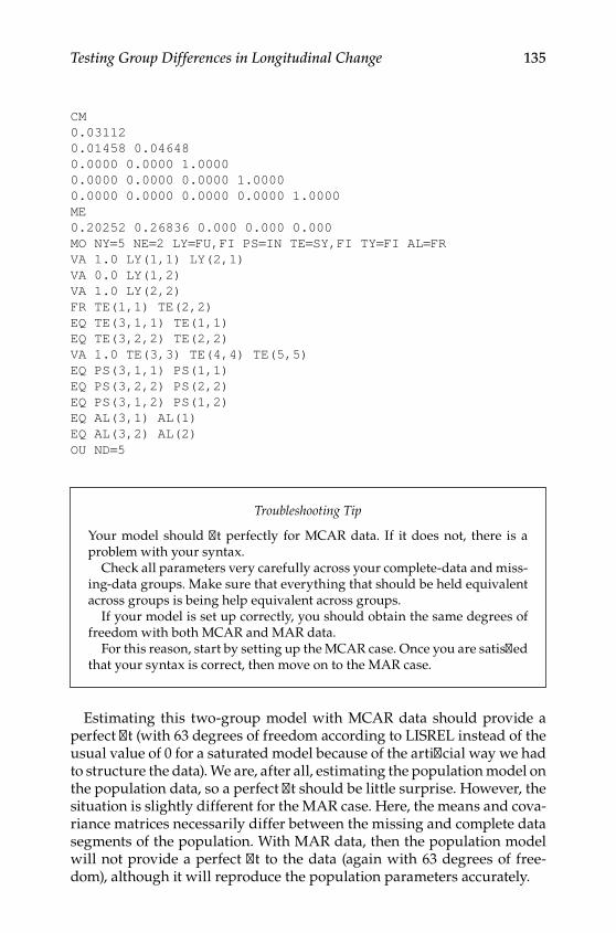
Testing Group Differences in Longitudinal Change 135
CM0.031120.01458 0.046480.0000 0.0000 1.00000.0000 0.0000 0.0000 1.00000.0000 0.0000 0.0000 0.0000 1.0000ME0.20252 0.26836 0.000 0.000 0.000MO NY=5 NE=2 LY=FU,FI PS=IN TE=SY,FI TY=FI AL=FRVA 1.0 LY(1,1) LY(2,1)VA 0.0 LY(1,2)VA 1.0 LY(2,2)FR TE(1,1) TE(2,2)EQ TE(3,1,1) TE(1,1)EQ TE(3,2,2) TE(2,2)VA 1.0 TE(3,3) TE(4,4) TE(5,5)EQ PS(3,1,1) PS(1,1)EQ PS(3,2,2) PS(2,2)EQ PS(3,1,2) PS(1,2)EQ AL(3,1) AL(1)EQ AL(3,2) AL(2)OU ND=5
Estimating this two‑group model with MCAR data should provide a perfect fit (with 63 degrees of freedom according to LISREL instead of the usual value of 0 for a saturated model because of the artificial way we had to structure the data). We are, after all, estimating the population model on the population data, so a perfect fit should be little surprise. However, the situation is slightly different for the MAR case. Here, the means and cova‑riance matrices necessarily differ between the missing and complete data segments of the population. With MAR data, then the population model will not provide a perfect fit to the data (again with 63 degrees of free‑dom), although it will reproduce the population parameters accurately.
Troubleshooting Tip
Your model should fit perfectly for MCAR data. If it does not, there is a problem with your syntax.
Check all parameters very carefully across your complete‑data and miss‑ing‑data groups. Make sure that everything that should be held equivalent across groups is being help equivalent across groups.
If your model is set up correctly, you should obtain the same degrees of freedom with both MCAR and MAR data.
For this reason, start by setting up the MCAR case. Once you are satisfied that your syntax is correct, then move on to the MAR case.
Y100315.indb 135 7/15/09 2:59:45 PM

136 Statistical Power Analysis with Missing Data
In order to run our alternative models, very few modifications to the population model are required. For example, to constrain the values of AL(2) equal across groups, we simply need to add the constraint
EQ AL(1,2) AL(2)
in the third group. No other changes are needed. Doing so for this spe‑cific example gives us a chi‑square value of 16.81551 with 64 degrees of freedom. Our second alternative model involves fixing PS(2,2) at half its population value (0.00146) and PS(1,2) at zero. We can do this by adding
FI PS(1,2) PS(2,2)
and
VA 0.00146 PS(2,2)
on the model lines in the first group. Doing so produces a chi‑square value of 173.12133 with 65 degrees of freedom.
We can now turn to an illustration of how this output can be used to conduct a power analysis or calculate a required sample size.
Step 7: using the results to Calculate Power or required Sample Size
LISREL calculates the value of the chi‑square statistic as (N − g) × FMin, where N is the total sample size, and g is the number of groups. Our population model has two groups, boys and girls, but with missing data we are forced to estimate a four‑group model. Thus, though the chi‑square value we obtain for a particular model depends in part on the number of patterns of missing data we have (and our sample size), FMin (labeled as Minimum Fit Function Value in LISREL) is independent of both these factors. We can thus estimate a particular pair of models once and obtain estimated values of the NCP for any sample size by calculating the difference in FMin between the population and alterna‑tive models and multiplying it by (N − g). For this example, with 50% missing data, the FMin values obtained for the test of equal means and trivial variance are 0.00842 and 0.08673, respectively. Table 7.3 shows the
Try Me!
Run the model above with your syntax, and ensure that your results agree before proceeding to Step 7.
Y100315.indb 136 7/15/09 2:59:45 PM
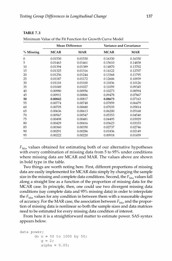
Testing Group Differences in Longitudinal Change 137
FMin values obtained for estimating both of our alternative hypotheses with every combination of missing data from 5 to 95% under conditions where missing data are MCAR and MAR. The values above are shown in bold type in the table.
Two things are worth noting here. First, different proportions of missing data are easily implemented for MCAR data simply by changing the sample size in the missing and complete data conditions. Second, the FMin values fall along a straight line as a function of the proportion of missing data for the MCAR case. In principle, then, one could use two divergent missing data conditions (say complete data and 95% missing data) in order to interpolate the FMin values for any condition in between them with a reasonable degree of accuracy. For the MAR case, the association between FMin and the propor‑tion of missing data is nonlinear so both the sample sizes and data matrices need to be estimated for every missing data condition of interest.
From here it is a straightforward matter to estimate power. SAS syntax appears below.
data power; do n = 50 to 1000 by 50; g = 2; alpha = 0.05;
Table 7.3
Minimum Value of the Fit Function for Growth Curve Model
Mean Difference Variance and Covariance
% Missing MCAR MAR MCAR MAR
0 0.01530 0.01530 0.16330 0.163305 0.01463 0.01461 0.15610 0.1483810 0.01394 0.01389 0.14870 0.1370215 0.01325 0.01316 0.14122 0.1270720 0.01256 0.01244 0.13368 0.1179525 0.01187 0.01172 0.12606 0.1093930 0.01118 0.01100 0.11836 0.1012635 0.01049 0.01027 0.11059 0.0934540 0.00980 0.00956 0.10273 0.0859445 0.00911 0.00886 0.09478 0.0786750 0.00842 0.00817 0.08673 0.0716355 0.00774 0.00748 0.07859 0.0647960 0.00705 0.00680 0.07035 0.0581465 0.00636 0.00613 0.06200 0.0516870 0.00567 0.00547 0.05353 0.0454075 0.00498 0.00481 0.04495 0.0392980 0.00429 0.00416 0.03623 0.0333385 0.00360 0.00350 0.02737 0.0274690 0.00291 0.00286 0.01836 0.0214995 0.00222 0.00220 0.00918 0.01459
Y100315.indb 137 7/15/09 2:59:45 PM

138 Statistical Power Analysis with Missing Data
df = 1; fmin = 0.011093 ncp = (n-g)*fmin; chicrit = quantile(‘chisquare’,1-alpha, 1); power = 1- PROBCHI(chicrit,df,ncp); output; end;proc print data=power; var n alpha df ncp power;run;
It is similarly straightforward to find a sample size required to yield the desired power for a given noncentrality parameter. We show how to do so simultaneously for degrees of freedom ranging from 1 to 10. Remember that the degrees of freedom for testing differences between latent slopes is tested with a single degree of freedom and that our simultaneous test of trivial slope variance and zero covariance with the intercept is tested with 2 degrees of freedom.
data ncp; alpha = 0.05; power = 0.80; fmin = 0.011093 do df = 1 to 10; chicrit = quantile(‘chisquare’,1-alpha, df); ncp = CINV(power, df, chicrit); output; end;proc print data=ncp; var df chicrit ncp;run;
We use the minimum values of the fit function shown in Table 7.3 to illustrate a sample result. Setting missing data on the last three waves of measurement at 50% we can plot the resulting statistical power for sample sizes from 100 to 1000 for each of our tests with the table entries shown in bold type. Figure 7.3 shows the estimated power for MCAR and MAR data to detect group differences (1 df test) and nontrivial variability in rates of change (2 df test) as a function of sample size.
As can be seen in Figure 7.4, which plots the results with 50% of obser‑vations missing, statistical power is only slightly greater for most sample sizes in this example when data are MCAR than MAR. In fact, they essen‑tially overlap for the test of mean differences. When the power is quite high, as it is for the test of the variance and covariance, adequate power can be achieved with fairly modest sample sizes and these rates of missing
Y100315.indb 138 7/15/09 2:59:45 PM
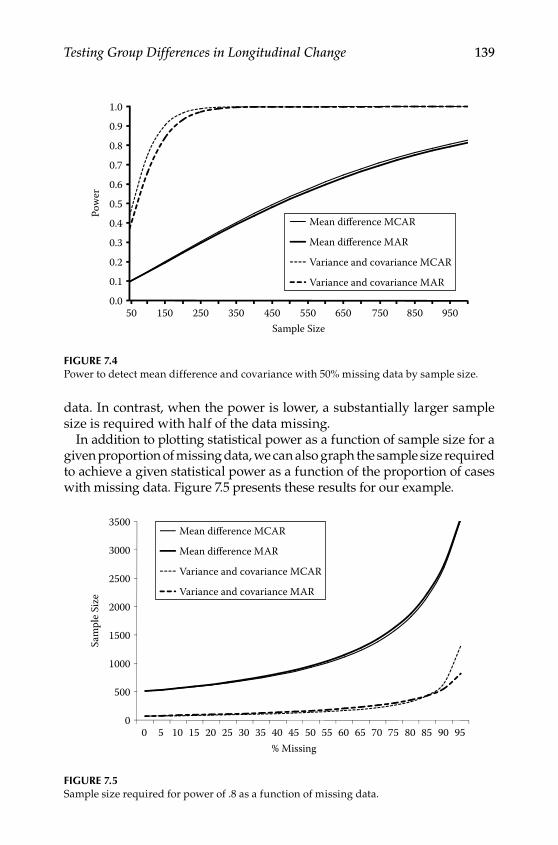
Testing Group Differences in Longitudinal Change 139
data. In contrast, when the power is lower, a substantially larger sample size is required with half of the data missing.
In addition to plotting statistical power as a function of sample size for a given proportion of missing data, we can also graph the sample size required to achieve a given statistical power as a function of the proportion of cases with missing data. Figure 7.5 presents these results for our example.
0.0
0.1
0.2
0.3
0.4
0.5
0.6
0.7
0.8
0.9
1.0Po
wer
Sample Size50 150 250 350 450 550 650 750 850 950
Mean difference MCAR
Mean difference MAR
Variance and covariance MCAR
Variance and covariance MAR
Figure 7.4Power to detect mean difference and covariance with 50% missing data by sample size.
0
500
1000
1500
2000
2500
3000
3500
Sam
ple S
ize
% Missing0 5 10 15 20 25 30 35 40 45 50 55 60 65 70 75 80 85 90 95
Mean difference MCAR
Mean difference MAR
Variance and covariance MCAR
Variance and covariance MAR
Figure 7.5Sample size required for power of .8 as a function of missing data.
Y100315.indb 139 7/15/09 2:59:46 PM
140 Statistical Power Analysis with Missing Data
Again, we find that there are ranges over which missing data can be increased considerably without requiring a substantially larger sample size to achieve the same statistical power, as indicated by the segments of each curve where the slope is quite low. Thus, the results we present are quite general and can be used for any combination of alpha, sample size, proportion missing data, and statistical power. Fixing two quantities at a desired value allows you to plot the other two against one another.
Conclusions
Using this approach and a given effect size, Type I error rate, and expected proportion of missing data, it is possible to estimate the statis‑tical power for any comparisons desired. In principle, there may be as many as 2k − 1 different patterns of missing data, where k is the number of variables.
With real data, however, it is common that a small number of patterns typically predominate, and patterns represented by small numbers of cases typically contribute negligibly to statistical power (cf. Dolan et al., 2005). Thus, the approach we outline here usually provides a sufficiently good first approximation for power calculations. In principle, as long as there are sufficient observations in a missing data pattern to calculate means, variances, and covariances, that pattern can be included in the model.
Even when this is not possible, many times these observations can be excluded without much additional loss of statistical power. Because it ensures that all model parameters are estimable, the number of cases in the complete data group is of single greatest importance. We recommend that researchers use caution with situations such as accelerated longitudi‑nal designs where there is not necessarily a complete‑data group. Nested model comparisons are still possible for designs such as this one, even though it may not be possible to estimate the standard saturated model. Most times, another suitable model can usually be identified which esti‑mates all possible moments, and this model can in turn serve as a baseline model for comparative purposes. In situations where a large number of different patterns of missing data is either expected or obtained, it usu‑ally makes the most sense to simulate raw data under a narrower range of conditions and use FIML estimation (L. K. Muthén & Muthén, 2002). We consider this situation in much greater detail in Chapter 9.
Y100315.indb 140 7/15/09 2:59:46 PM

Testing Group Differences in Longitudinal Change 141
Further Readings
Curran, P. J., & Muthén, B. O. (1999). The application of latent curve analysis to testing developmental theories in intevention research. American Journal of Community Psychology, 27, 567–595.
Davey, A., & Savla, J. (2009). Estimating statistical power with incomplete data. Organizational Research Methods, 12, 320–346.
Exercises
1. Using the population parameters from Figure 7.3 and the matrices that follow, calculate the power to detect a significant mean differ‑ence and variance with complete data using three, four, and five waves of data.
2. Using the same models, find the sample size required to achieve power of .8 with 25% MCAR missing data on the last wave in each case.
3. Repeat the same process assuming that the probability of data being missing on the last observation is a function of the first observation (i.e., for the five‑wave model, w = [ ]).1 0 0 0 0
Y100315.indb 141 7/15/09 2:59:47 PM

Y100315.indb 142 7/15/09 2:59:47 PM

143
8Effects of Following Up via Different Patterns When Data Are Randomly or Systematically Missing
In this chapter, we consider several examples of statistical power in plan‑ning a study with data missing by design. The empirical example is a slightly simplified version of the model presented in the previous chapter. Using three‑wave longitudinal data, we evaluate four different planned missingness designs. As with the preceding chapter, we consider both missing completely at random (MCAR) and missing at random (MAR) data as well as a wide range of sample sizes. We conclude the chapter with a general way to evaluate pattern missingness that can be useful in planning a study with data that are missing by design. We will revisit and extend several of these design issues again in Chapter 10.
Background
There are a number of situations where researchers set out in advance to collect only partial information from a portion of their sample. In surveys, for example, screening items may be used to determine the appropriate range of follow up questions. Many large‑scale national surveys such as the Health and Retirement Study (Juster & Suzman, 1995) include “modules” to which random subsamples of individuals from the entire survey are assigned. Likewise, we have already considered several historical “incom‑plete” designs, such as Solomon’s four‑group design, Latin squares designs (Campbell & Stanley, 1963), the accelerated longitudinal design (Bell, 1954), various “sequential” designs, and McArdle’s (1994) fractional blocks design. Other more modern incarnations of these intentionally incomplete approaches include adaptive testing (e.g., Weiss & Kingsbury, 1984), where responses on previous questions are used to determine the selection of subsequent items (see Collins et al., 2004, for an application of adaptive methods to the preventive intervention context). Used appropriately, this
Y100315.indb 143 7/15/09 2:59:47 PM

144 Statistical Power Analysis with Missing Data
approach can considerably reduce testing burden that would otherwise be associated with estimating ability to a desired level of accuracy.
Another area of research, however, actively sets out to collect partial data from some or all individuals. Graham et al. (1996), for example, intro‑duced something they called the XABC design, which has several varia‑tions. All individuals may get form X, for example, with one third also receiving forms A and B, one third receiving forms A and C, and one third receiving forms B and C. Because no participant receives all four forms, there is no guarantee that all parameters will be estimable, so it may be more desirable to divide the sample into quarters, with one quarter receiv‑ing all four forms in addition to a quarter of participants being assigned to each of the other three incomplete conditions. If assignment is made on a purely random basis, then the data are, by definition, missing completely at random. Thus, they can be combined and analyzed using techniques such as full information maximum likelihood or multiple imputations without additional concern.
Graham, Taylor, and Cumsille (2001) elaborated upon this approach to extend it to longitudinal data, as well as considering the possibility of having a larger number of conditions, and circumstances that might be more amenable to less costly but also less rigorous designs (Graham, Taylor, Orchowski, & Cumsille, 2006). To date, although there has been little systematic research on the potential ways in which intentionally assigning individuals to different longitudinal data collection conditions might itself affect nonresponse (cf. Davey, 2001), the principles at least are sound. Graham and his colleagues (2001) considered a number of different designs and evaluated statistical power (as standard errors) with regard to considerations such as costs per measurement. Their approach suggests that some designs will be inherently more efficient than others, and so any potential design should be selected carefully as a result of an a priori power analysis using methods such as the ones we describe here.
The approach outlined in this volume may also be of particular use when planning for data that will be inherently missing, such as in acceler‑ated longitudinal designs. T. E. Duncan, Duncan, and Hops (1996) pres‑ent an especially clear example of this type of design in the context of structural equation modeling. In addition to estimating statistical power for the overall model parameters of primary interest (such as changes in latent means or inter‑individual variability in rates of change), our approach can (and should) be used to estimate power to test assumptions regarding appropriate use of the accelerated longitudinal design. Primary among these, for example, are tests of convergence (E. R. Anderson, 1993; Bell, 1953, 1954; T. E. Duncan et al., 1996), specifically that overlapping seg‑ments of the overall trajectory can actually be equated across cohorts (or, in the context of power analysis, rejected when the assumption is indeed violated to varying degrees). Likewise, researchers can evaluate issues
Y100315.indb 144 7/15/09 2:59:47 PM
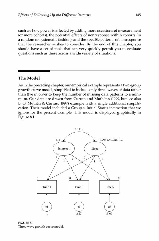
Effects of Following Up via Different Patterns 145
such as: how power is affected by adding more occasions of measurement (or more cohorts), the potential effects of nonresponse within cohorts (in a random or systematic fashion), and the specific patterns of nonresponse that the researcher wishes to consider. By the end of this chapter, you should have a set of tools that can very quickly permit you to evaluate questions such as these across a wide variety of situations.
The Model
As in the preceding chapter, our empirical example represents a two‑group growth curve model, simplified to include only three waves of data rather than five in order to keep the number of missing data patterns to a mini‑mum. Our data are drawn from Curran and Muthén’s (1999, but see also B. O. Muthén & Curran, 1997) example with a single additional simplifi‑cation. Their model included a Group × Initial Status interaction that we ignore for the present example. This model is displayed graphically in Figure 8.1.
0
Time 1
0
Time 3
0
Time 5
1, 1
Intercept
0.798 or 0.981, 0.2
Slope
,1
e1
,2.27
e3
,5.09
e5
11 1 0
12
0.1118
Figure 8.1Three‑wave growth curve model.
Y100315.indb 145 7/15/09 2:59:47 PM
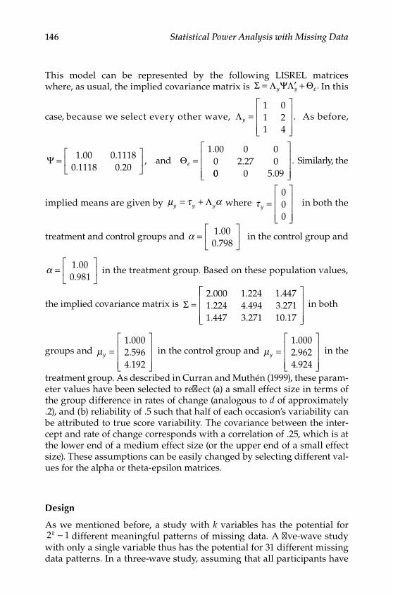
146 Statistical Power Analysis with Missing Data
This model can be represented by the following LISREL matrices where, as usual, the implied covariance matrix is Σ Λ ΨΛ Θ= ′ +y y ε . In this
case, because we select every other wave, Λy =
1 01 21 4
. As before,
Ψ Θ=
=1 00 0 1118
0 1118 0 20
1 00 0 00 2 27 0
. .. .
,.
.and ε
00 0 5 09..
Similarly, the
implied means are given by µ τ αy y y= + Λ where τ y =
000
in both the
treatment and control groups and α =
1 000 798
..
in the control group and
α =
1 000 981
..
in the treatment group. Based on these population values,
the implied covariance matrix is Σ =2 000 1 224 1 4471 224 4 494 3 2711 447 3 271 10 17
. . .
. . .
. . .
in both
groups and µy =
1 0002 5964 192
.
.
. in the control group and µy =
1 0002 9624 924
.
.
. in the
treatment group. As described in Curran and Muthén (1999), these param‑eter values have been selected to reflect (a) a small effect size in terms of the group difference in rates of change (analogous to d of approximately .2), and (b) reliability of .5 such that half of each occasion’s variability can be attributed to true score variability. The covariance between the inter‑cept and rate of change corresponds with a correlation of .25, which is at the lower end of a medium effect size (or the upper end of a small effect size). These assumptions can be easily changed by selecting different val‑ues for the alpha or theta‑epsilon matrices.
Design
As we mentioned before, a study with k variables has the potential for 2 1k − different meaningful patterns of missing data. A five‑wave study with only a single variable thus has the potential for 31 different missing data patterns. In a three‑wave study, assuming that all participants have
Y100315.indb 146 7/15/09 2:59:49 PM
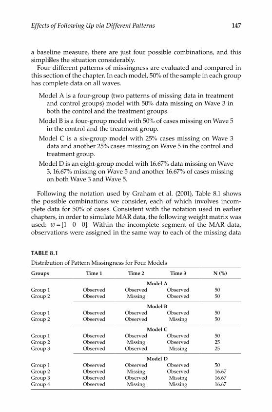
Effects of Following Up via Different Patterns 147
a baseline measure, there are just four possible combinations, and this simplifies the situation considerably.
Four different patterns of missingness are evaluated and compared in this section of the chapter. In each model, 50% of the sample in each group has complete data on all waves.
Model A is a four‑group (two patterns of missing data in treatment and control groups) model with 50% data missing on Wave 3 in both the control and the treatment groups.
Model B is a four‑group model with 50% of cases missing on Wave 5 in the control and the treatment group.
Model C is a six‑group model with 25% cases missing on Wave 3 data and another 25% cases missing on Wave 5 in the control and treatment group.
Model D is an eight‑group model with 16.67% data missing on Wave 3, 16.67% missing on Wave 5 and another 16.67% of cases missing on both Wave 3 and Wave 5.
Following the notation used by Graham et al. (2001), Table 8.1 shows the possible combinations we consider, each of which involves incom‑plete data for 50% of cases. Consistent with the notation used in earlier chapters, in order to simulate MAR data, the following weight matrix was used: w = [ ].1 0 0 Within the incomplete segment of the MAR data, observations were assigned in the same way to each of the missing data
Table 8.1
Distribution of Pattern Missingness for Four Models
Groups Time 1 Time 2 Time 3 N (%)
Model AGroup 1 Observed Observed Observed 50Group 2 Observed Missing Observed 50
Model BGroup 1 Observed Observed Observed 50Group 2 Observed Observed Missing 50
Model CGroup 1 Observed Observed Observed 50Group 2 Observed Missing Observed 25Group 3 Observed Observed Missing 25
Model DGroup 1 Observed Observed Observed 50Group 2 Observed Missing Observed 16.67Group 3 Observed Observed Missing 16.67Group 4 Observed Missing Missing 16.67
Y100315.indb 147 7/15/09 2:59:50 PM
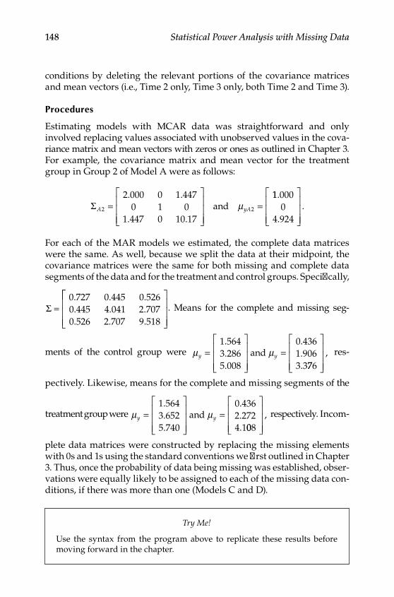
148 Statistical Power Analysis with Missing Data
conditions by deleting the relevant portions of the covariance matrices and mean vectors (i.e., Time 2 only, Time 3 only, both Time 2 and Time 3).
Procedures
Estimating models with MCAR data was straightforward and only involved replacing values associated with unobserved values in the cova‑riance matrix and mean vectors with zeros or ones as outlined in Chapter 3. For example, the covariance matrix and mean vector for the treatment group in Group 2 of Model A were as follows:
ΣA yA2 2
2 000 0 1 4470 1 0
1 447 0 10 17=
=. .
. .and µ
11 0000
4 924
.
..
For each of the MAR models we estimated, the complete data matrices were the same. As well, because we split the data at their midpoint, the covariance matrices were the same for both missing and complete data segments of the data and for the treatment and control groups. Specifically,
Σ =0 727 0 445 0 5260 445 4 041 2 7070 526 2 707 9 518
. . .
. . .
. . .
. Means for the complete and missing seg‑
ments of the control group were µ µy y=
=1 5643 2865 008
0 4361 9063 3
.
.
.
.
.
.and
776
, res‑
pectively. Likewise, means for the complete and missing segments of the
treatment group were µ µy y=
=1 5643 6525 740
0 4362 2724 1
.
.
.
.
.
.and
008
, respectively. Incom‑
plete data matrices were constructed by replacing the missing elements with 0s and 1s using the standard conventions we first outlined in Chapter 3. Thus, once the probability of data being missing was established, obser‑vations were equally likely to be assigned to each of the missing data con‑ditions, if there was more than one (Models C and D).
Try Me!
Use the syntax from the program above to replicate these results before moving forward in the chapter.
Y100315.indb 148 7/15/09 2:59:50 PM
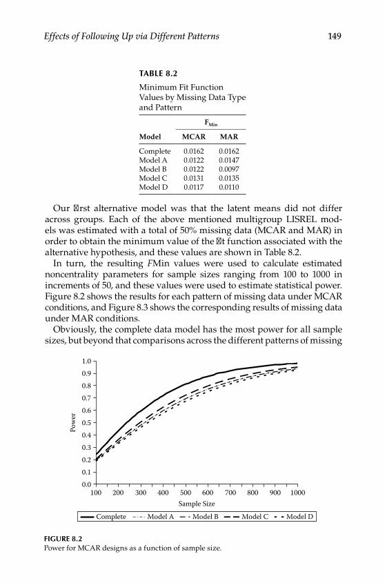
Effects of Following Up via Different Patterns 149
Our first alternative model was that the latent means did not differ across groups. Each of the above mentioned multigroup LISREL mod‑els was estimated with a total of 50% missing data (MCAR and MAR) in order to obtain the minimum value of the fit function associated with the alternative hypothesis, and these values are shown in Table 8.2.
In turn, the resulting FMin values were used to calculate estimated noncentrality parameters for sample sizes ranging from 100 to 1000 in increments of 50, and these values were used to estimate statistical power. Figure 8.2 shows the results for each pattern of missing data under MCAR conditions, and Figure 8.3 shows the corresponding results of missing data under MAR conditions.
Obviously, the complete data model has the most power for all sample sizes, but beyond that comparisons across the different patterns of missing
Table 8.2
Minimum Fit Function Values by Missing Data Type and Pattern
FMin
Model MCAR MAR
Complete 0.0162 0.0162Model A 0.0122 0.0147Model B 0.0122 0.0097Model C 0.0131 0.0135Model D 0.0117 0.0110
0.00.10.20.30.40.50.60.70.80.91.0
Sample Size100 200 300 400 500 600 700 800 900 1000
Pow
er
Complete Model A Model B Model C Model D
Figure 8.2Power for MCAR designs as a function of sample size.
Y100315.indb 149 7/15/09 2:59:51 PM
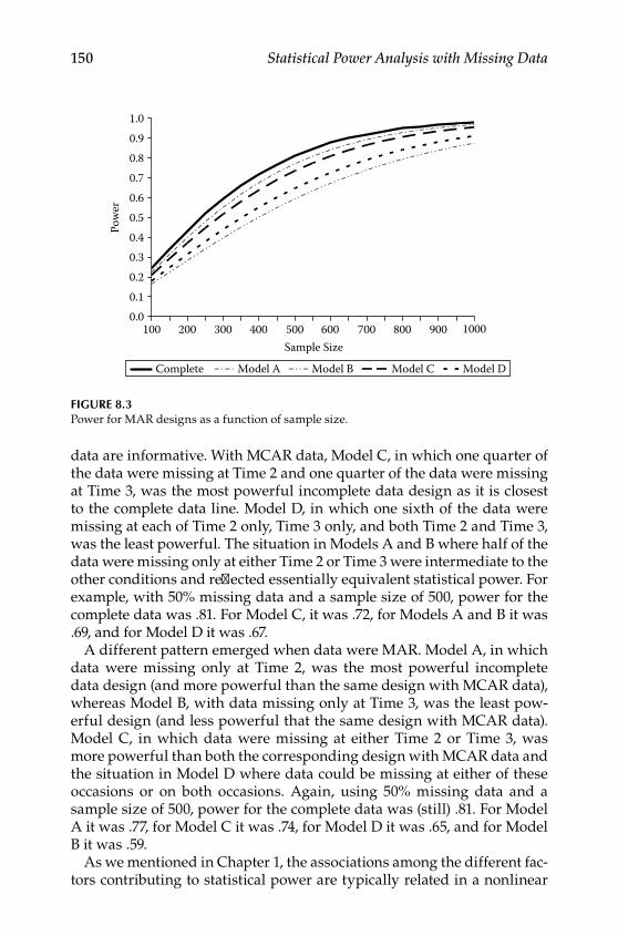
150 Statistical Power Analysis with Missing Data
data are informative. With MCAR data, Model C, in which one quarter of the data were missing at Time 2 and one quarter of the data were missing at Time 3, was the most powerful incomplete data design as it is closest to the complete data line. Model D, in which one sixth of the data were missing at each of Time 2 only, Time 3 only, and both Time 2 and Time 3, was the least powerful. The situation in Models A and B where half of the data were missing only at either Time 2 or Time 3 were intermediate to the other conditions and reflected essentially equivalent statistical power. For example, with 50% missing data and a sample size of 500, power for the complete data was .81. For Model C, it was .72, for Models A and B it was .69, and for Model D it was .67.
A different pattern emerged when data were MAR. Model A, in which data were missing only at Time 2, was the most powerful incomplete data design (and more powerful than the same design with MCAR data), whereas Model B, with data missing only at Time 3, was the least pow‑erful design (and less powerful that the same design with MCAR data). Model C, in which data were missing at either Time 2 or Time 3, was more powerful than both the corresponding design with MCAR data and the situation in Model D where data could be missing at either of these occasions or on both occasions. Again, using 50% missing data and a sample size of 500, power for the complete data was (still) .81. For Model A it was .77, for Model C it was .74, for Model D it was .65, and for Model B it was .59.
As we mentioned in Chapter 1, the associations among the different fac‑tors contributing to statistical power are typically related in a nonlinear
0.00.10.20.30.40.50.60.70.80.91.0
Pow
er
Complete Model A Model B Model C Model D
Sample Size100 200 300 400 500 600 700 800 900 1000
Figure 8.3Power for MAR designs as a function of sample size.
Y100315.indb 150 7/15/09 2:59:51 PM
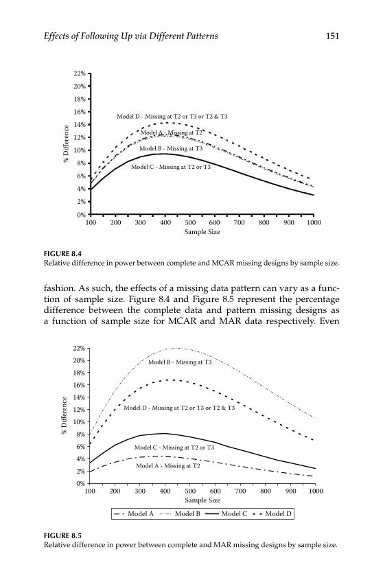
Effects of Following Up via Different Patterns 151
fashion. As such, the effects of a missing data pattern can vary as a func‑tion of sample size. Figure 8.4 and Figure 8.5 represent the percentage difference between the complete data and pattern missing designs as a function of sample size for MCAR and MAR data respectively. Even
Model D - Missing at T2 or T3 or T2 & T3
22%
20%
18%
16%
14%
12%
10%
8%
6%
% D
iffer
ence
4%
2%
0%100 200 300 400 500
Sample Size600 700 800 900 1000
Model A - Missing at T2
Model B - Missing at T3
Model C - Missing at T2 or T3
Figure 8.4Relative difference in power between complete and MCAR missing designs by sample size.
0%2%4%6%8%
10%12%14%16%18%20%22%
Sample Size100 200 300 400 500 600 700 800 900 1000
% D
iffer
ence
Model C - Missing at T2 or T3
Model B - Missing at T3
Model A - Missing at T2
Model D - Missing at T2 or T3 or T2 & T3
Model A Model B Model C Model D
Figure 8.5Relative difference in power between complete and MAR missing designs by sample size.
Y100315.indb 151 7/15/09 2:59:52 PM

152 Statistical Power Analysis with Missing Data
though half the sample in each case has missing observations, the differ‑ence between complete and missing data designs never exceeds 22% and for most sample sizes is less than 15%. Likewise, the proportional difference in power increases with sample sizes up to a sample size of — depending on the design — around 400, after which the proportional differences again decrease. Where this point occurs will vary as a function of the model and the effect size (as well as the mechanism underlying the missing data). If planning a large study, this suggests that the loss of statistical power as a result of incorporating a missing data design may be quite minimal for many purposes. In the next section, we consider ways to extend this approach to planning a missing data design.
evaluating Missing Data Patterns
The maximum likelihood formula we first introduced in Chapter 2 to calculate model noncentrality parameters and FMin values can be readily extended to include means. Specifically, to compare a null (F0) and alter‑native (FA) model, the likelihood ratio chi‑square test statistic can be cal‑culated as
χ µ µ2 10 0 0
1= × + ( ) ×( ) − − − −( )′ ×− −N Trace pA A A Aln lnΣ Σ Σ Σ Σ ×× −( )
µ µ0 A
where N (or N − 1) is the number of observations, and p is the number of observed variables. This equation looks intimidating, but taken one term at a time, every piece reduces down to a scalar value. As such, it amounts to nothing more than addition and subtraction of a series of numbers, multiplied by the sample size. Satorra and Saris (1985) showed how this value provided an estimate of the noncentrality parameter (λ) when esti‑mating the alternative model, FA, with population data, F0. This equation can also be extended to multiple groups or patterns of data, which we will illustrate below.
C. Dolan, van der Sluis, and Grasman (2005) provided a useful exten‑sion of the pattern missingness approach in the MCAR case. We will also
Point of Reflection
Graham and colleagues (2001) considered the power of studies with planned missingness as a function of cost per observation. From this perspective, it is possible to construct costs for each pattern within a design in order to optimize power given costs. Given that not all observations are created equal in terms of time or money, you may wish to consider this approach when planning your own research.
Y100315.indb 152 7/15/09 2:59:52 PM
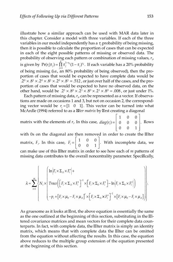
Effects of Following Up via Different Patterns 153
illustrate how a similar approach can be used with MAR data later in this chapter. Consider a model with three variables. If each of the three variables in our model independently has a tj probability of being missing, then it is possible to calculate the proportion of cases that can be expected in each of the eight possible patterns of missing or observed data. The probability of observing each pattern or combination of missing values, ri,
is given by Pr( | ) ( ) .ri jj
p
jr
jrij ijτ τ τ= ∏ −
=
−
1
1 1 If each variable has a 20% probability
of being missing (i.e., an 80% probability of being observed), then the pro‑portion of cases that would be expected to have complete data would be . . . . . . .2 8 2 8 2 8 5120 1 0 1 0 1× × × × × = , or just over half of the cases, and the pro‑portion of cases that would be expected to have no observed data, on the other hand, would be . . . . . . .2 8 2 8 2 8 0081 0 1 0 1 0× × × × × = , or just under 1%.
Each pattern of missing data, ri, can be represented as a vector. If observa‑tions are made on occasions 1 and 3, but not on occasion 2, the correspond‑ing vector would be ri = [ ]1 0 1 . This vector can be turned into what McArdle (1994) referred to as a filter matrix by first creating a diagonal
matrix with the elements of ri. In this case, diag ri( ) .=
1 0 00 0 00 0 1
Rows
with 0s on the diagonal are then removed in order to create the filter
matrix, Fi. In this case, Fi =
1 0 00 0 1
. With incomplete data, we
can make use of this filter matrix in order to see how each of m patterns of missing data contributes to the overall noncentrality parameter. Specifically,
λ ≈ ×
× × ′ +
× × ′
× × × ′
−N
F F
Trace F F F Fi
i A i
i A i i i
ln Σ
Σ Σ1
0
− × × ′
− + × − ×[ ]′ × ×
ln F F
p F F F
i i
i i i A i A
Σ
Σ
0
0µ µ ×× ′
× × − ×[ ]
−F F Fi i i A
1
0µ µ
=∑i
m
1
.
As gruesome as it looks at first, the above equation is essentially the same as the one outlined at the beginning of this section, substituting in the fil‑tered covariance matrices and mean vectors for their complete data coun‑terparts. In fact, with complete data, the filter matrix is simply an identity matrix, which means that with complete data the filter can be omitted from the equation without affecting the results. In this case, the equation above reduces to the multiple group extension of the equation presented at the beginning of this section.
Y100315.indb 153 7/15/09 2:59:54 PM
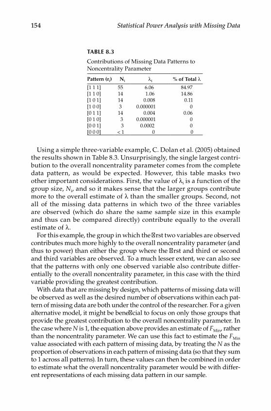
154 Statistical Power Analysis with Missing Data
Using a simple three‑variable example, C. Dolan et al. (2005) obtained the results shown in Table 8.3. Unsurprisingly, the single largest contri‑bution to the overall noncentrality parameter comes from the complete data pattern, as would be expected. However, this table masks two other important considerations. First, the value of λi is a function of the group size, Ni, and so it makes sense that the larger groups contribute more to the overall estimate of λ than the smaller groups. Second, not all of the missing data patterns in which two of the three variables are observed (which do share the same sample size in this example and thus can be compared directly) contribute equally to the overall estimate of λ.
For this example, the group in which the first two variables are observed contributes much more highly to the overall noncentrality parameter (and thus to power) than either the group where the first and third or second and third variables are observed. To a much lesser extent, we can also see that the patterns with only one observed variable also contribute differ‑entially to the overall noncentrality parameter, in this case with the third variable providing the greatest contribution.
With data that are missing by design, which patterns of missing data will be observed as well as the desired number of observations within each pat‑tern of missing data are both under the control of the researcher. For a given alternative model, it might be beneficial to focus on only those groups that provide the greatest contribution to the overall noncentrality parameter. In the case where N is 1, the equation above provides an estimate of FMin, rather than the noncentrality parameter. We can use this fact to estimate the FMin value associated with each pattern of missing data, by treating the N as the proportion of observations in each pattern of missing data (so that they sum to 1 across all patterns). In turn, these values can then be combined in order to estimate what the overall noncentrality parameter would be with differ‑ent representations of each missing data pattern in our sample.
Table 8.3
Contributions of Missing Data Patterns to Noncentrality Parameter
Pattern (ri) Ni λi % of Total λ[1 1 1] 55 6.06 84.97[1 1 0] 14 1.06 14.86[1 0 1] 14 0.008 0.11[1 0 0] 3 0.000001 0[0 1 1] 14 0.004 0.06[0 1 0] 3 0.000001 0[0 0 1] 3 0.0002 0[0 0 0] < 1 0 0
Y100315.indb 154 7/15/09 2:59:54 PM

Effects of Following Up via Different Patterns 155
To illustrate how this approach might be used, let us simplify our model even further by focusing on a single_group model. As before, Λy, Ψ, Θe, and ty will be the same as in our original model. For this example, however,
we will use α =
00 197.
, which is the difference between the two origi‑
nal groups and, by design, reflects a small effect size. Two simple alterna‑tive hypotheses that can be tested are that the parameter associated with longitudinal change does not differ from 0 (i.e., the groups change in simi‑lar ways), or that the intercept and rate of change are uncorrelated. In the population the correlation was equivalent to .25, which is at the low end of a medium effect size. We work through Stata syntax to evaluate these to estimate these values, presenting one section at a time. Syntax for other software packages can be found in the Appendix.
First, we specify the population covariance structure.
#delimit;matrix ly0 = (1, 0 \ 1, 2 \ 1, 4 );matrix ps0 = (1, .1118 \ .1118, .2 );matrix te0 = (1, 0, 0 \ 0, 2.27, 0 \ 0, 0, 5.09 );matrix ty0 = (0 \ 0 \ 0 );matrix al0 = (1 \ .197);matrix sigma0 = ly0*ps0*ly0’ + te0;matrix muy0 = ty0 + ly0*al0;
Next, we specify the alternative model. The following syntax would be used to test whether the change parameter differs from zero.
matrix ly1 = (1, 0 \ 1, 2 \ 1, 4 );matrix ps1 = (1, .1118 \ .1118, .2 );matrix te1 = (1, 0, 0 \ 0, 2.27, 0 \ 0, 0, 5.09 );matrix ty1 = (0 \ 0 \ 0 );matrix al1 = (1 \ 0);matrix sigma1 = ly1*ps1*ly1’ + te1;matrix muy1 = ty1 + ly1*al1;
Y100315.indb 155 7/15/09 2:59:54 PM

156 Statistical Power Analysis with Missing Data
Likewise, the following syntax can be used to specify the implied covariance matrix and vector of means if the intercept and slope are uncorrelated.
matrix ly1 = (1, 0 \ 1, 2 \ 1, 4 );matrix ps1 = (1, 0 \ 0, .2 );matrix te1 = (1, 0, 0 \ 0, 2.27, 0 \ 0, 0, 5.09 );matrix ty1 = (0 \ 0 \ 0 );matrix al1 = (1 \ .197);matrix sigma1 = ly1*ps1*ly1’ + te1;matrix muy1 = ty1 + ly1*al1;
With complete data, the minimum value of the fit function (FMin) can be estimated as follows. Here, all we have done is translate the equa‑tion from the beginning of the chapter into some fairly straightforward arithmetic.
matrix p = rowsof(sigma0);matrix n = (1);matrix fmin = trace(n)*(ln(det(sigma1)) +
trace(inv(sigma1)*sigma0) - ln(det(sigma0)) –trace(p) +trace((muy0 - muy1)’*inv(sigma1)*(muy0 - muy1)));
Each pattern of missing data can be specified using a filter matrix. To specify each possible pattern of missing data where two of the three occasions are observed, the corresponding filter matrices would be F1,2 =
1 0 00 1 0
1 0 00 0 1
0 1 00 0 11 3 2 3
=
=
, ,, ,F Fand
.
To specify
each possible pattern of missing data where only one of the three occasionswas observed, the corresponding filter matrices would be F1 = [1 0 0],F2 0 1 0= [ ], and F3 0 0 1= [ ]. Estimating the corresponding FMin val‑ues for each pattern of incomplete data is then straightforward with syn‑tax like the following.
matrix filter = (1, 0, 0 \ 0, 1, 0 );matrix subsigma0 = filter*sigma0*filter’;matrix submuy0 = filter*muy0;
Y100315.indb 156 7/15/09 2:59:55 PM
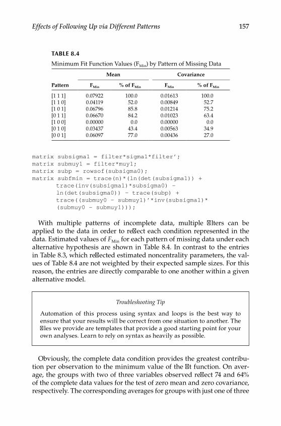
Effects of Following Up via Different Patterns 157
matrix subsigma1 = filter*sigma1*filter’;matrix submuy1 = filter*muy1;matrix subp = rowsof(subsigma0);matrix subfmin = trace(n)*(ln(det(subsigma1)) + trace(inv(subsigma1)*subsigma0) – ln(det(subsigma0)) - trace(subp) + trace((submuy0 - submuy1)’*inv(subsigma1)* (submuy0 - submuy1)));
With multiple patterns of incomplete data, multiple filters can be applied to the data in order to reflect each condition represented in the data. Estimated values of FMin for each pattern of missing data under each alternative hypothesis are shown in Table 8.4. In contrast to the entries in Table 8.3, which reflected estimated noncentrality parameters, the val‑ues of Table 8.4 are not weighted by their expected sample sizes. For this reason, the entries are directly comparable to one another within a given alternative model.
Obviously, the complete data condition provides the greatest contribu‑tion per observation to the minimum value of the fit function. On aver‑age, the groups with two of three variables observed reflect 74 and 64% of the complete data values for the test of zero mean and zero covariance, respectively. The corresponding averages for groups with just one of three
Table 8.4
Minimum Fit Function Values (FMin) by Pattern of Missing Data
Mean Covariance
Pattern FMin % of FMin FMin % of FMin
[1 1 1] 0.07922 100.0 0.01613 100.0[1 1 0] 0.04119 52.0 0.00849 52.7[1 0 1] 0.06796 85.8 0.01214 75.2[0 1 1] 0.06670 84.2 0.01023 63.4[1 0 0] 0.00000 0.0 0.00000 0.0[0 1 0] 0.03437 43.4 0.00563 34.9[0 0 1] 0.06097 77.0 0.00436 27.0
Troubleshooting Tip
Automation of this process using syntax and loops is the best way to ensure that your results will be correct from one situation to another. The files we provide are templates that provide a good starting point for your own analyses. Learn to rely on syntax as heavily as possible.
Y100315.indb 157 7/15/09 2:59:55 PM
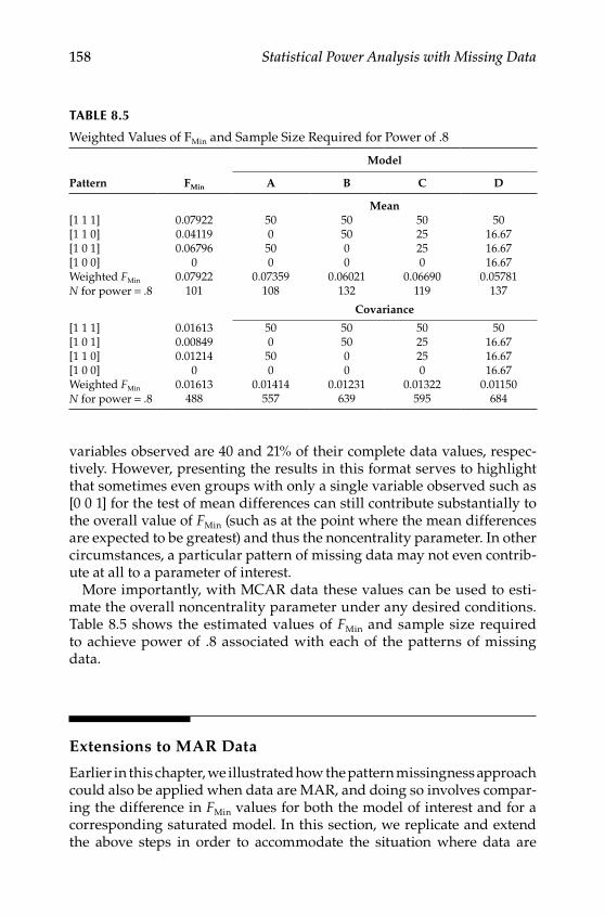
158 Statistical Power Analysis with Missing Data
variables observed are 40 and 21% of their complete data values, respec‑tively. However, presenting the results in this format serves to highlight that sometimes even groups with only a single variable observed such as [0 0 1] for the test of mean differences can still contribute substantially to the overall value of FMin (such as at the point where the mean differences are expected to be greatest) and thus the noncentrality parameter. In other circumstances, a particular pattern of missing data may not even contrib‑ute at all to a parameter of interest.
More importantly, with MCAR data these values can be used to esti‑mate the overall noncentrality parameter under any desired conditions. Table 8.5 shows the estimated values of FMin and sample size required to achieve power of .8 associated with each of the patterns of missing data.
Extensions to MAR Data
Earlier in this chapter, we illustrated how the pattern missingness approach could also be applied when data are MAR, and doing so involves compar‑ing the difference in FMin values for both the model of interest and for a corresponding saturated model. In this section, we replicate and extend the above steps in order to accommodate the situation where data are
Table 8.5
Weighted Values of FMin and Sample Size Required for Power of .8
Model
Pattern FMin A B C D
Mean[1 1 1] 0.07922 50 50 50 50[1 1 0] 0.04119 0 50 25 16.67[1 0 1] 0.06796 50 0 25 16.67[1 0 0] 0 0 0 0 16.67Weighted FMin 0.07922 0.07359 0.06021 0.06690 0.05781N for power = .8 101 108 132 119 137
Covariance
[1 1 1] 0.01613 50 50 50 50[1 0 1] 0.00849 0 50 25 16.67[1 1 0] 0.01214 50 0 25 16.67[1 0 0] 0 0 0 0 16.67Weighted FMin 0.01613 0.01414 0.01231 0.01322 0.01150N for power = .8 488 557 639 595 684
Y100315.indb 158 7/15/09 2:59:55 PM

Effects of Following Up via Different Patterns 159
MAR instead of MCAR. Doing so is complicated somewhat further by the fact that selection affects both the observed and missing portions of the data as well as, by necessity, the proportions in each group. For this reason, we present fairly general syntax that can easily be modified very simply in order to consider different proportions of complete and incom‑plete data, as well as various null and alternative models. Consideration of planned missing data under the MAR situation may be desirable in situations where, for example, testing burden is likely to be an issue (such as with frail older adults), when suggested by another aspect of the study design (such as where follow‑ups are planned on the basis of screening items or criterion scores) or where the costs associated with following up certain subgroups are likely to be prohibitive (such as for those moving out of state).
After defining the null and alternative models as in the MCAR case, the next step is to specify the selection process. Using the same three‑wave single‑group model, selection for MAR data is based upon data from the first occasion, which will be observed for all individuals. Sample syntax to define the variable associated with selection is straightforward.
* Create Selected and Unselected Matrices;* Pr(Miss) = f(T1 Only);matrix w = (1, 0, 0 );* Mean of Selection Variable;matrix mus0 = w*muy0;* Variance of Selection Variable;matrix vars0 = w*sigma0*w’;* Standard Deviation of Selection Variable;matrix sds0 = cholesky(vars0);
The next section calculates the required interim values associated with selection, which are needed to calculate the effects of the selection process on the means and covariance structure in the selected and unselected seg‑ments of the population. Changing the proportion of missing or complete data can be accomplished by changing the value of probmiss or changing from a specific value to a loop over the range of interest.
* Mean and variance in selected subsample;matrix probmiss = (.5);matrix d = invnorm(trace(probmiss));matrix phis = normalden(trace(d));matrix PHIs = normal(trace(d));matrix xPHIs = I(1) - PHIs;matrix muss0 = mus0 + sds0*phis*inv(xPHIs);matrix musu0 = mus0 - sds0*phis*inv(PHIs);
Y100315.indb 159 7/15/09 2:59:55 PM

160 Statistical Power Analysis with Missing Data
matrix varss0 = vars0*(1 + (d*phis*inv(xPHIs)) – (phis*phis*inv(xPHIs)*inv(xPHIs)));matrix varsu0 = vars0*(1 – (d*phis*inv(PHIs)) – (phis*phis*inv(PHIs)*inv(PHIs)));matrix omegas0 = inv(vars0)*(varss0 – vars0)*inv(vars0);matrix omegau0 = inv(vars0)*(varsu0 – vars0)*inv(vars0);matrix sigmas0 = sigma0 + omegas0*(sigma0*(w’*w)*sigma0);matrix sigmau0 = sigma0 + omegau0*(sigma0*(w’*w)*sigma0);matrix ks0 = inv(vars0)*(muss0 - mus0);matrix ku0 = inv(vars0)*(musu0 - mus0);matrix muys0 = muy0 + sigma0*w’*ks0;matrix muyu0 = muy0 + sigma0*w’*ku0;
As with the MCAR example, we define the filter variables associated with complete and missing data conditions. In this case, the syntax assumes that values in the incomplete data group are observed on the first two occasions but not at the third.
* Now Create Appropriate Comparisons;* Original Data;matrix p = rowsof(sigma0);matrix n = (1);matrix fmin= trace(n)*(ln(det(sigma1)) + trace(inv(sigma1)*sigma0) - ln(det(sigma0)) – trace(p) + trace((muy0 - muy1)’*inv(sigma1)*(muy0 - muy1)));* Complete Data Filter;matrix cfilter = (1, 0, 0 \ 0, 1, 0 \ 0, 0, 1 );* Missing Data Filter;matrix mfilter = (1, 0, 0 \ 0, 1, 0 );
The first comparison with MAR data is between the selected data matri‑ces with the values implied by the alternative model, just as it would be with MCAR data. We create each of the (filtered) submatrices required for this comparison.
* First Compare Selected and Unselected with H1;matrix subsigma0s = cfilter*sigmas0*cfilter’;matrix submuy0s = cfilter*muys0;
Y100315.indb 160 7/15/09 2:59:55 PM

Effects of Following Up via Different Patterns 161
matrix subsigma1c = cfilter*sigma1*cfilter’;matrix submuy1c = cfilter*muy1;matrix subsigma0u = mfilter*sigmau0*mfilter’;matrix submuy0u = mfilter*muyu0;matrix subsigma1m = mfilter*sigma1*mfilter’;matrix submuy1m = mfilter*muy1;matrix subpc = rowsof(subsigma0s);matrix nc = (I(1) - probmiss);matrix subpm = rowsof(subsigma0u);matrix nm = (probmiss);
Based on these values, the contribution to FMin values can be calculated separately for the complete and incomplete portions of the data. Notice that we define the sample size for the complete and missing components of the data in terms of probmiss. Changing its value will automatically change not only the matrices implied under the selection model but also the proportions of complete and missing observations in the model. In order to accommodate multiple patterns of incomplete data (or different cut‑points as described in Chapter 3), the proportion of incomplete obser‑vations can also be modified. To replicate Model D, for example, nm could be divided by 3 for each of the three patterns of incomplete data, each of which would also have its own filter matrix. All other aspects of the esti‑mation procedure would be the same.
matrix fminc1 = trace(nc)*(ln(det(subsigma1c)) + trace(inv(subsigma1c)*subsigma0s) – ln(det(subsigma0s)) – trace(subpc) + trace((submuy0s - submuy1c)’*inv(subsigma1c)* (submuy0s - submuy1c)));matrix fminm1 = trace(nm)*(ln(det(subsigma1m)) + trace(inv(subsigma1m)*subsigma0u) – ln(det(subsigma0u)) - trace(subpm) + trace((submuy0u - submuy1m)’*inv(subsigma1m)* (submuy0u - submuy1m)));
In Chapter 3, we noted that for MAR data there were two sources of discrepancies between the population and alternative models. The first comes from the fact that the alternative model is false in the population, and the second comes from the selection process itself. The covariance matrices and mean vectors will always differ in the top and bottom seg‑ments of the population whenever selection is systematic. To subtract out this second source of discrepancy, we also need to estimate the true popu‑lation model on the selected and unselected segments of the population. The following syntax calculated the additional required quantities and
Y100315.indb 161 7/15/09 2:59:55 PM

162 Statistical Power Analysis with Missing Data
estimates the corresponding discrepancy between the observed values and what they would have been in the absence of selection.
* Next Compare Selected and Unselected with H0;matrix subsigma0c = cfilter*sigma0*cfilter’;matrix submuy0c = cfilter*muy0;matrix subsigma0m = mfilter*sigma0*mfilter’;matrix submuy0m = mfilter*muy0;matrix fminc0 = trace(nc)*(ln(det(subsigma0c)) + trace(inv(subsigma0c)*subsigma0s) – ln(det(subsigma0s)) - trace(subpc) + trace((submuy0s - submuy0c)’*inv(subsigma0c)* (submuy0s - submuy0c)));matrix fminm0 = trace(nm)*(ln(det(subsigma0m)) + trace(inv(subsigma0m)*subsigma0u) – ln(det(subsigma0u)) - trace(subpm) + trace((submuy0u - submuy0m)’*inv(subsigma0m)* (submuy0u - submuy0m)));
An overall estimate of the adjusted FMin value can now be obtained directly.
matrix fminall = (fminc1 + fminm1) – (fminc0 + fminm0);
It is also easy to calculate this value as a proportion of what the corre‑sponding complete data value would have been, as the following state‑ment does:
matrix pctfmin = 100*fminall*inv(fmin);
Table 8.6 shows the values of FMin across the range of incomplete data from 5 to 95% with Models A and B for tests of 0 mean and 0 covariance, respectively. Under all circumstances, statistical power is reduced with incomplete data, relative to the complete data condition. However, what is notable is that the rate of proportional rate of change in the FMin values is typically much less than the rate of change in missing data. Even when half of the sample has incomplete data on the third observation, the FMin is still at least three quarters of its complete data value. How important this difference is for statistical power is a function of the sample size and under many circumstances may be quite small. Considering a range of patterns of missing data and a range of hypotheses will convey a sense of the implications that missing data are likely to have for key hypotheses of interest and the circumstances where the effects of incomplete data are likely to be greater or smaller. For both of the alternative hypotheses con‑sidered here, Model A provides larger values of FMin than does Model B and is thus the more powerful design.
Y100315.indb 162 7/15/09 2:59:56 PM
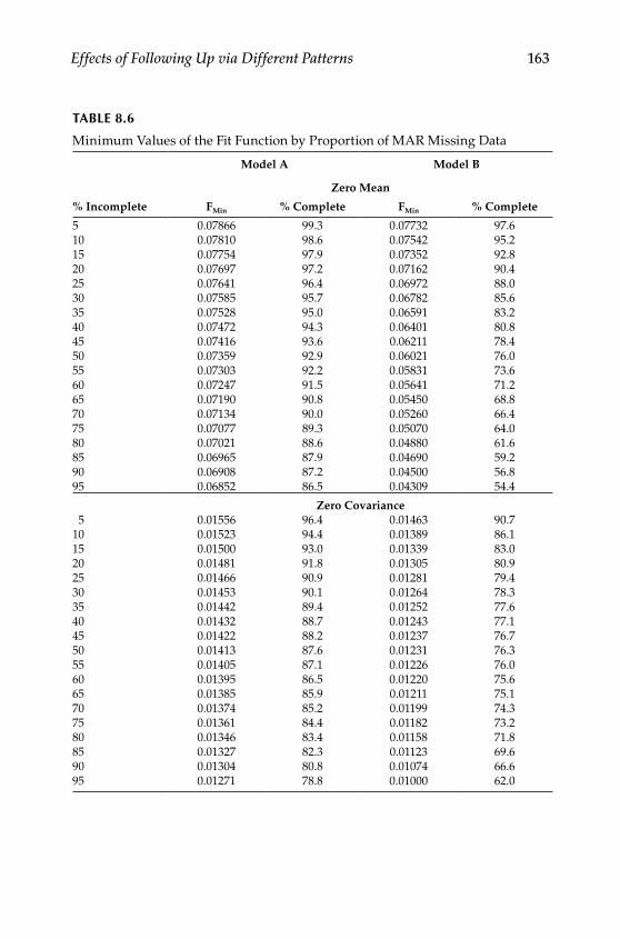
Effects of Following Up via Different Patterns 163
Table 8.6
Minimum Values of the Fit Function by Proportion of MAR Missing Data
Model A Model B
Zero Mean
% Incomplete FMin % Complete FMin % Complete
5 0.07866 99.3 0.07732 97.610 0.07810 98.6 0.07542 95.215 0.07754 97.9 0.07352 92.820 0.07697 97.2 0.07162 90.425 0.07641 96.4 0.06972 88.030 0.07585 95.7 0.06782 85.635 0.07528 95.0 0.06591 83.240 0.07472 94.3 0.06401 80.845 0.07416 93.6 0.06211 78.450 0.07359 92.9 0.06021 76.055 0.07303 92.2 0.05831 73.660 0.07247 91.5 0.05641 71.265 0.07190 90.8 0.05450 68.870 0.07134 90.0 0.05260 66.475 0.07077 89.3 0.05070 64.080 0.07021 88.6 0.04880 61.685 0.06965 87.9 0.04690 59.290 0.06908 87.2 0.04500 56.895 0.06852 86.5 0.04309 54.4
Zero Covariance 5 0.01556 96.4 0.01463 90.710 0.01523 94.4 0.01389 86.115 0.01500 93.0 0.01339 83.020 0.01481 91.8 0.01305 80.925 0.01466 90.9 0.01281 79.430 0.01453 90.1 0.01264 78.335 0.01442 89.4 0.01252 77.640 0.01432 88.7 0.01243 77.145 0.01422 88.2 0.01237 76.750 0.01413 87.6 0.01231 76.355 0.01405 87.1 0.01226 76.060 0.01395 86.5 0.01220 75.665 0.01385 85.9 0.01211 75.170 0.01374 85.2 0.01199 74.375 0.01361 84.4 0.01182 73.280 0.01346 83.4 0.01158 71.885 0.01327 82.3 0.01123 69.690 0.01304 80.8 0.01074 66.695 0.01271 78.8 0.01000 62.0
Y100315.indb 163 7/15/09 2:59:56 PM

164 Statistical Power Analysis with Missing Data
Conclusions
In this chapter, we focused attention on situations where data will be missing by design. These “managed missingness” situations are impor‑tant because several large‑scale surveys now include incomplete data and also because of situations where it may be desirable to plan to col‑lect incomplete data from the outset. There are many situations where time considerations require that partial data be collected from some or all individuals, and the strategies outlined in the current chapter provide a set of tools that can be used to evaluate missing data designs in terms of key study hypotheses. The strategies we outline can be applied across a variety of null and alternative models, a wide array of incomplete patterns of incomplete data, as well as data which are MCAR or MAR. Because the rate of decrease in the minimum value of the fit function is likely in many cases to be less than the rate of decrease in missing observations, with careful planning, the most efficient design may be one that includes data missing by design. In the next chapter, we extend these ideas to situ‑ations where it may be desirable to simulate raw data, either to consider situations with a large number of patterns of missing data or in order to evaluate the effects of violating various assumptions on statistical power with incomplete data.
Further Readings
Graham, J. W., Hofer, S. M., & MacKinnon, D. P. (1996). Maximizing the useful‑ness of data obtained with planned missing value patterns: An application of maximum likelihood procedures. Multivariate Behavioral Research, 31, 197–218.
Graham, J. W., Taylor, B. J., & Cumsille, P. E. (2001). Planned missing data designs in analysis of change. In L. Collins & A. Sayer (Eds.), New methods for the analysis of change (pp. 335–353). Washington, DC: American Psychological Association.
Exercises
1. Use the first three waves of the model from Figure 7.3 (and exer‑cises from Chapter 7) to replicate the entries in Table 8.3.
2. Use the entries from your version of Table 8.3 to replicate the entries in Table 8.4.
3. How would these values differ if you used waves 1, 3, and 5 from Figure 7.3 for MCAR data?
Y100315.indb 164 7/15/09 2:59:56 PM

165
9Using Monte Carlo Simulation Approaches to Study Statistical Power With Missing Data
To this point, we have concerned ourselves with the range of analytic contexts in which sufficient statistics such as means, variances, and covariances were all that was necessary to estimate statistical power. This approach, however, only begins to scratch the surface of situa‑tions that may be of interest to the applied researcher. By extending our consideration of statistical power with missing data to include Monte Carlo simulation studies with raw data, the range of applications and situations that can be evaluated is greatly expanded. In this chapter, we begin by very briefly considering some guidelines for planning and implementing a Monte Carlo simulation study, along with references to more detailed sources. Next, we present some of the different ways of generating raw data for use in a Monte Carlo study. The latter part of this chapter is devoted to exploring some applications of Monte Carlo meth‑ods with missing data, such as evaluating convergence rates, assessing model fit statistics, complex missing data patterns, and violations of model assumptions.
Planning and Implementing a Monte Carlo Study
Monte Carlo methods provide a probabilistic solution for problems where exact calculations are typically either not possible to obtain (or very diffi‑cult to obtain) or are not necessary to obtain because they can more easily be well approximated. Consider the problem of trying to determine the area of one shape relative to another. In the case of Figure 9.1, we have a circle nested within a square. In this case, the edges of the circle exactly touch the edges of the square. Because both shapes have known formulas
Y100315.indb 165 7/15/09 2:59:56 PM

166 Statistical Power Analysis with Missing Data
for their areas and we have some way to relate those areas, we can solve the problem easily and exactly. The area of the square is A lSquare = 2 , where l is the length of its sides. The area of the square is ACircle
l= π( ) .22 With both
of these expressions, we can say that the proportion of the square that isoccupied by the circle is π
4 or a little more than 78%. The problems we have considered to this point are similar to this one.
In contrast, consider Figure 9.2. Solving the ratio of areas of these two shapes is much more difficult because we have little a priori information helping us relate one area to another and the area of the inner shape is highly irregular and would be difficult to characterize with a formula. A Monte Carlo approach to finding the ratio of the areas would be quite straightforward. We could print out a copy of the shapes, pin it to the wall, and then proceed to throw darts at the wall. We would count up the num‑ber of darts that landed inside the lightning bolt, the number of shapes that landed in the square but outside the lightning bolt, and any darts that missed the square entirely either (a) would not be counted, or (b) would be thrown at the wall again until all of the darts were somewhere in the square.
The proportion of darts landing inside the lightning bolt would approx‑imate the proportion of the square’s area occupied by the lightning bolt: Shazam! This approach would also work with the circle in Figure 9.1. One advantage of this approach is that it allows to us to solve even rather difficult problems quite simply. The downside, however, is that this can be a fairly labor‑intensive approach. To increase the accuracy of our approximate
Figure 9.1Example of a problem that can be solved exactly.
Y100315.indb 166 7/15/09 2:59:57 PM

Using Monte Carlo Simulation Approaches to Study Statistical Power 167
solution, it is necessary to “throw more darts,” often 10,000 or more. As ever, there is no free lunch. The researcher is trading off between a small number of very difficult calculations versus a very large number of much simpler calculations. With a computer, we would use a random number generator to provide us with two uncorrelated variables (say x and y) that would uniformly cover the area of the square, which we could represent as all pairs of coordinates between 0 and 1 on the x‑axis and y‑axis.
Both structural equation modeling with incomplete data and statisti‑cal power analysis are situations that are ideally suited for this kind of approach. In contrast to the situations that have been presented to this point in the volume, the Monte Carlo approach provides the opportunity to consider more complex situations (typically under a more limited set of conditions) as well as how a model is likely to perform in practice as opposed to in principle. As such, Monte Carlo methods can provide a very useful “brute force” complement to the broader approaches we have out‑lined to this point. For other problems, they may represent the only cur‑rently practical solution.
Researchers interested in learning about Monte Carlo methods will find no shortage of sources to consult for advice and examples and an article by Metropolis (1987) provides a very interesting history of the method. Fan, Felsővályi, Sivo, and Keenan (2001), for example, provide a readily accessible introduction to conducting basic Monte Carlo studies using SAS. Within a structural equation modeling framework, Bandalos (2006) provides a thoughtful introduction to Monte Carlo research that covers the most important considerations such as design and the range
Figure 9.2Example of a problem than can be solved only approximately.
Y100315.indb 167 7/15/09 2:59:57 PM

168 Statistical Power Analysis with Missing Data
of outcomes that are most often considered. Paxton and colleagues (2001) outline a number of very useful guidelines for getting started with Monte Carlo research, and Skrondal (2000) provides additional considerations for increasing the potential external validity of results generated from a Monte Carlo study. As well, many empirical studies of different aspects of structural equation modeling rely on Monte Carlo methods and provide a good resource for researchers interested in implementing these meth‑ods (e.g., Enders & Bandalos, 2001; Fan, 2003; Gerbing & Anderson, 1993; Hu & Bentler, 1999; L. K. Muthén & Muthén, 2002; Sivo & Willson, 2000; Arbuckle, 1996).
Paxton and colleagues (2001) provide some very specific guidelines for planning and conducting a Monte Carlo study within the structural equa‑tion modeling framework, identifying nine key steps, as listed in Table 9.1. What follows in this section corresponds directly with the guidelines offered by Paxton and colleagues, because their recommendations are so generally applicable.
It is critical that every Monte Carlo study begin with a theoretically informed research question. If there is little compelling theoretical rea‑son to investigate a phenomenon, then the results are unlikely to have much scientific value. This step also helps to guide the range of conditions that are worth investigation. External validity is also a key consideration in designing a Monte Carlo study. Ensuring that the model under inves‑tigation has relevance to the kind of situations typically studied in the structural equation modeling framework increases the potential value of a Monte Carlo study. Using published research to guide the selection of models is a great place to start in this regard.
Selection of the specific conditions that will be manipulated by the researcher is also of critical importance. Typical choices to be considered
Table 9.1
Paxton and Colleagues’ Steps in Planning a Monte Carlo Study
Step Task
1 Developing a research question derived from theory2 Creating a valid model3 Designing (selecting) experimental conditions4 Selecting values of population parameters5 Selecting an appropriate software package6 Conducting the simulations7 File storage8 Troubleshooting and verification9 Summarizing results
Y100315.indb 168 7/15/09 2:59:57 PM

Using Monte Carlo Simulation Approaches to Study Statistical Power 169
include variables such as the sample size, number of latent and manifest indicators, method of estimation, type and extent of model misspecifi‑cation, type and extent of missing data, and of course the distributions of the raw data. Once the conditions themselves have been selected, it is also necessary to select appropriate values of the population param‑eters, such as factor loadings and structural coefficients. Given the facto‑rial nature of most experimental designs, the number of factors grows geometrically, even before considering the desired number of replications for each condition. Again, theory and the empirical literature can help to guide the specific factors and their levels that should be considered in any simulation study. This trade‑off between the number of conditions under investigation and the number of replications considered was one of the factors that led Skrondal (2000) to question the “conventional wisdom” on designing Monte Carlo studies. His perspective is that researchers should consider a wider range of conditions using fewer replications under each condition in order to increase the potential external validity of any spe‑cific study. Though most Monte Carlo studies consider fixed values (e.g., specific sample sizes) of study factors, there is generally no reason that they could not be treated as random factors, where generalizability is the primary concern.
Choice of an appropriate software package for conducting a simulation study is also an important consideration. Each program presents its own strengths and limitations, but the primary consideration should be ease and accuracy with which the researcher can conduct the actual study. Programs differ with regard to the ease with which they can accom‑modate factors such as data generation, level of measurement, analysis of multiple replication, and storage and presentation of results. As of the time of this writing, for example, LISREL will allow analysis of replicated data with missing data using full information maximum likelihood esti‑mation but is extremely limited in the output it allows researchers to save. AMOS provides an easy interface for Monte Carlo analyses through pro‑gramming with Visual Basic. MPlus and EQS both provide quite flexible opportunities to generate and analyze both normal and nonnormal data internally. For any given application, and any given researcher, however, it may be just as convenient to generate the data using one software pack‑age, estimate models in another, and analyze the results in still another. Ease of moving between different data formats also reduces potential bar‑riers in this regard.
Next on the list of steps is the actual execution of the Monte Carlo study. Paxton et al. (2001) point to additional considerations at this stage, such as whether to include nonconverged replications in the results. (They recom‑mend against it in order to keep the number of replications equal across
Y100315.indb 169 7/15/09 2:59:57 PM

170 Statistical Power Analysis with Missing Data
conditions unless rates of nonconvergence are of explicit interest, such as in the study by Enders & Bandalos, 2001.) Others have varied the number of replications across different sample size conditions in order to hold the total number of observations in each condition constant. If improper solu‑tions are to be excluded, then additional data sets must be generated to allow for models that do not converge or that provide improper solutions. All of these analyses can place considerable demands on both computa‑tion time and storage resources, and plans need to be made in advance for how data will be retained and archived. Fortunately, storage media have become quite economical, greatly reducing the burden of this aspect of conducting a Monte Carlo study.
The final two steps outlined by Paxton and colleagues (2001) are check‑ing the results (we recommend doing this early and often) and summa‑rizing the results. With regard to the former, we recommend routinely obtaining descriptive and bivariate statistics for the data under each of the study conditions in order to ensure that they have been appropriately gen‑erated and read by the software packages. In our simulation studies we do so if possible in each of the software packages used. Ensure that the cor‑rect number of observations and data sets have been read; verify that the model is correctly structured and estimated; leave nothing to chance. In terms of summarizing results, Paxton et al. recommend using a combina‑tion of descriptive, graphical, and inferential approaches, and their advice is difficult to argue with. Because of the vast quantity of results generated within the typical simulation study, we particularly recommend learn‑ing more about compact and effective ways to communicate information visually (e.g., Tufte, 2001), along with methods for exploratory data analy‑sis (e.g., Tukey, 1977).
Simulating Raw Data Under a Population Model
In any computer simulation setting, it is important to recognize that (a) numbers generated by a computer are not truly random, (b) in order to be replicable, an initial “seed” value must be specified, and (c) over
Point of Reflection
What are some important topics in your own area of research which might lend themselves to a Monte Carlo study? Can you find examples in the litera‑ture of situations where a simulation approach has been used? What are some of the key outcomes and factors that might be important for such a study?
Y100315.indb 170 7/15/09 2:59:57 PM
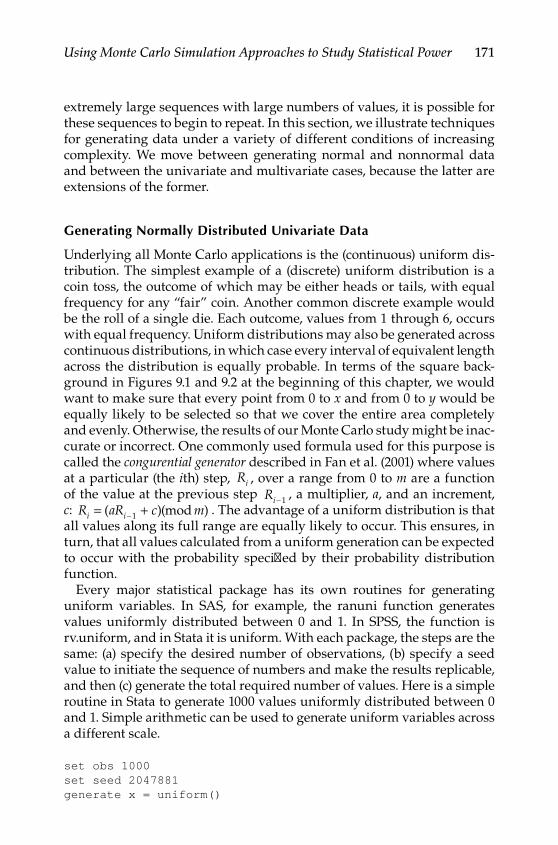
Using Monte Carlo Simulation Approaches to Study Statistical Power 171
extremely large sequences with large numbers of values, it is possible for these sequences to begin to repeat. In this section, we illustrate techniques for generating data under a variety of different conditions of increasing complexity. We move between generating normal and nonnormal data and between the univariate and multivariate cases, because the latter are extensions of the former.
generating Normally Distributed univariate Data
Underlying all Monte Carlo applications is the (continuous) uniform dis‑tribution. The simplest example of a (discrete) uniform distribution is a coin toss, the outcome of which may be either heads or tails, with equal frequency for any “fair” coin. Another common discrete example would be the roll of a single die. Each outcome, values from 1 through 6, occurs with equal frequency. Uniform distributions may also be generated across continuous distributions, in which case every interval of equivalent length across the distribution is equally probable. In terms of the square back‑ground in Figures 9.1 and 9.2 at the beginning of this chapter, we would want to make sure that every point from 0 to x and from 0 to y would be equally likely to be selected so that we cover the entire area completely and evenly. Otherwise, the results of our Monte Carlo study might be inac‑curate or incorrect. One commonly used formula used for this purpose is called the congurential generator described in Fan et al. (2001) where values at a particular (the ith) step, Ri , over a range from 0 to m are a function of the value at the previous step Ri−1 , a multiplier, a, and an increment, c: R aR c mi i= +−( )(mod )1 . The advantage of a uniform distribution is that all values along its full range are equally likely to occur. This ensures, in turn, that all values calculated from a uniform generation can be expected to occur with the probability specified by their probability distribution function.
Every major statistical package has its own routines for generating uniform variables. In SAS, for example, the ranuni function generates values uniformly distributed between 0 and 1. In SPSS, the function is rv.uniform, and in Stata it is uniform. With each package, the steps are the same: (a) specify the desired number of observations, (b) specify a seed value to initiate the sequence of numbers and make the results replicable, and then (c) generate the total required number of values. Here is a simple routine in Stata to generate 1000 values uniformly distributed between 0 and 1. Simple arithmetic can be used to generate uniform variables across a different scale.
set obs 1000set seed 2047881generate x = uniform()
Y100315.indb 171 7/15/09 2:59:58 PM

172 Statistical Power Analysis with Missing Data
The choice of a seed is important only in that syntax run with the same seed will produce identical results every time it is run, whereas syntax run without a seed (or with a different seed) will produce different out‑put. Although its importance depends on the type of random number gen‑erator used in a specific software package, it is generally good practice to select an odd‑numbered value for the seed. Once we have our uniformly distributed variables, we can readily transform them or use them to cal‑culate variables with other distributions. If a variable with a range from 1 to 100 is desired, we can calculate it as 99*x + 1 for example. A normally distributed variable with a mean of 50 and standard deviation of 10 can be calculated in Stata as 50 + 10*invnorm(x).
generating Nonnormally Distributed univariate Data
Using linear transformations such as the one above, researchers can con‑struct variables with any desired means and standard deviations, the first and second moments of a distribution. Often, researchers may wish to generate variables with nonnormal distributions, ones that also have known skewness and kurtosis. One of the most commonly used ways to accomplish this was outlined by Fleishman (1978). For desired values of skewness and kurtosis, his iterative method allows solving a set of equa‑tions for three values that can be used to transform a normally distributed variable into one with the desired values. Although his method involves quite a bit of algebra and numerous calculations (all best left to comput‑ers), the approach itself is not difficult to grasp.
Fleishman (1978) set out to find an approximation, using a polynomial transformation, of a normally distributed variable, X, into a nonnormally distributed variable, Y , with given skewness and kurtosis. In particular, Y a bX cX dX= + + +2 3, and the constants a , b , c , and d are solved for in terms of the moments of a normal distribution, which are known. Two simplifying assumptions are used, specifically that the mean is 0 and the standard deviation is 1. Linear transformations can be used after the fact to create variables with the desired mean and standard deviations. Setting the mean equal to 0 implies that a c+ = 0 (or, equivalently, that a c= − ). Setting the variance equal to 1 implies that b bd c d2 2 26 2 15 1+ + + = . The desired skewness (γ1) can be expressed in terms of the coefficients as γ 1
2 22 24 105 2= + + +c b bd d( ) . Similarly, the kurtosis (γ2) can be expre‑ssed as γ 2
2 2 2 224 1 28 12 48 141 225= + + + + + + +[ ( ) (bd c b bd d bd c dd2 )] . Now all that has to be done is to solve these four equations for the constants a, b, c, and d. One fairly straightforward way to do this is to find a solution using iterative techniques such as Newton’s method. Newton’s method
Y100315.indb 172 7/15/09 3:00:00 PM

Using Monte Carlo Simulation Approaches to Study Statistical Power 173
finds an approximate solution (within any desired level of accuracy) based on an initial starting value, x0 . The updated value at a given step is givenby x xn n
f xf x
n
n+( )′( )= −1 where f xn( ) is the value of the function at the nth itera‑
tion, and ′f xn( ) is the value of the first derivative of the function at the nth iteration. This process continues until x xn n+ − <1 the desired level of accuracy (or until the maximum number of iterations is reached). In this case, the process is conducted simultaneously for b , c , and d using matrix algebra by taking the partial derivatives of the equations above with respect to each unknown. A sample program that executes this pro‑cess using Stata appears below. By default, it is set up to continue until none of the parameters changes by more than 0.000001 or until 500 itera‑tions, whichever comes first.
/* Solving for Fleishman’s Coefficients */#delimit;mat maxiter = (500);mat iter = (0);* Skewness and Kurtosis;mat skewkurt = (1, 5);mat skew = skewkurt[1..rowsof(skewkurt),1];mat kurt = skewkurt[1..rowsof(skewkurt),2];mat output = J(rowsof(skewkurt),3,0);mat coef = (1 \ 0 \ 0);mat f = J(3,1,1);
while (trace(iter) <= trace(maxiter) &max(abs(f[1,1]),abs(f[2,1]),abs(f[3,1])) > .000001 {;mat b = coef[1,1];mat c = coef[2,1];mat d = coef[3,1];* Matrix of Function (f);mat f = (b*b+6*b*d+2*c*c+15*d*d - 1 \ 2*c*(b*b+24*b*d+105*d*d+2) - skew[4,1] \ 24*(b*d+c*c*(1+b*b+28*b*d)+d*d*(12+48*b*d+141*c*c+225*d*d)) - kurt[4,1]); * Matrix of Partial Derivatives (df); mat df = (2*b+6*d, 4*c, 6*b+30*d \ 4*c*(b+12*d), 2*(b*b+24*b*d+105*d*d+2), 4*c*(12*b+105*d) \ 24*(d+c*c*(2*b+28*d)+48*d*d), 48*c*(1+b*b+28*b*d+141*d*d),
24*(b+28*b*c*c+2*d*(12+48*b*d+141*c*c+225*d*d)+d*d)+d*d*(48 *b+450*d));
Y100315.indb 173 7/15/09 3:00:02 PM

174 Statistical Power Analysis with Missing Data
mat delta = inv(df)*f;
mat coef = coef - delta; mat iter=iter+I(1); }; mat list iter; mat list coef; mat list delta; mat list f; mat list df;
Not all combinations of skewness and kurtosis can be generated using this method. Specifically, whenever γ γ1
2220 0629576 0 0717247< × +. . ,
there is no solution. In these cases, approaches based on different meth‑ods must be used (e.g., Burr, 1942; Headrick & Mugdadi, 2006; Ramberg & Schmeiser, 1974).
generating Normally Distributed Multivariate Data
It is a fairly straightforward matter to generate multivariate normally distributed data with a desired covariance structure. Two methods, Cholesky decomposition and the factor pattern matrix, are used most commonly, both of which create linear combinations of independent (i.e., uncorrelated) normally distributed variables to construct new variables with the desired covariance structure.
Cholesky decomposition of a square symmetric matrix, S, uses a form of Gaussian elimination to find a lower triangular matrix, L, such that S = LL′ . In this way, it is analogous to the square root function in scalar algebra. Statistical packages with matrix routines such as SPSS, SAS, and Stata all have Cholesky decomposition commands (called chol, root, and cholesky, respectively). The same solution may also be obtained in struc‑tural equation modeling software such as LISREL very simply. Consider estimating the model in Figure 9.3.
We use the Cholesky‑decomposed matrix to take three uncorrelated variables (Old 1, Old 2, and Old 3) and estimate three new correlated vari‑ables (New 1, New 2, and New 3). New 1 is a linear function of Old 1; New 2 is a linear function of Old 1 and Old 2; New 3 is a linear function of Old 1, Old 2, and Old 3. In the LISREL model, we can estimate the lower trian‑gular matrix L using the following matrices.
Ψ Λ=
=
1 0 00 1 00 0 1
0 00,
** ** * *
,y andd Θε =
0 0 00 0 00 0 0
Y100315.indb 174 7/15/09 3:00:02 PM

Using Monte Carlo Simulation Approaches to Study Statistical Power 175
This model can be estimated from our desired covariance matrix, S =1 0 0 4 0 50 4 1 0 0 60 5 0 6 1 0
. . .
. . .
. . .,
in order to solve for L. In this case, L y= Λ because
LL S′ = .
da ni=3 no=1000lanew1 new2 new3cm1.4 1.5 .6 1mo ny=3 ne=3 ly=fu,fi be=fu,fi ps=sy,fi te=sy,fileold1 old2 old3va 1.0 ps(1,1) ps(2,2) ps(3,3)fr ly(1,1) ly(2,2) ly(3,3)fr ly(2,1) ly(3,1)fr ly(3,2)ou nd=4
Old 3Old 1 Old 2
New 3New 1 New 2
* *
* * * *
Figure 9.3Graphical representation of the Cholesky decomposition to generate variables with desired covariance structure from uncorrelated variables.
Y100315.indb 175 7/15/09 3:00:03 PM
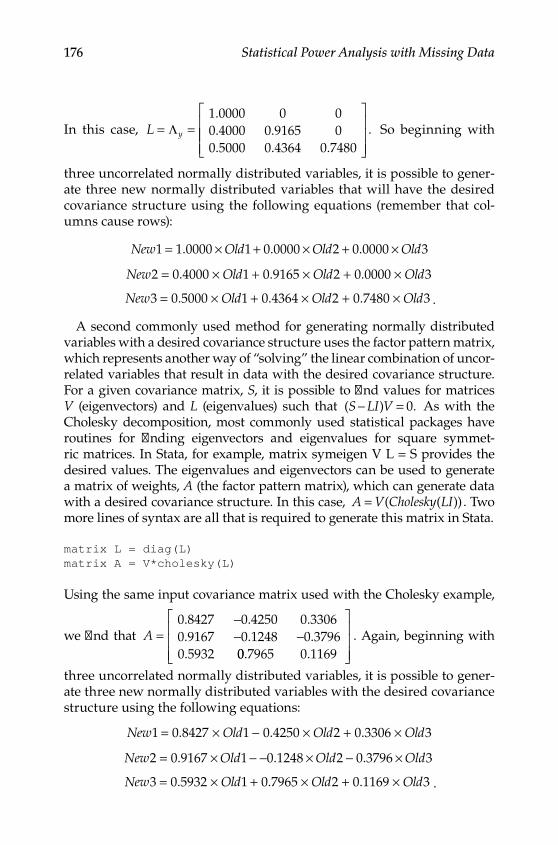
176 Statistical Power Analysis with Missing Data
In this case, L y= =
Λ1 0000 0 00 4000 0 9165 00 5000 0 4364 0 7480
.
. .
. . .
. So beginning with
three uncorrelated normally distributed variables, it is possible to gener‑ate three new normally distributed variables that will have the desired covariance structure using the following equations (remember that col‑umns cause rows):
New Old Old Old1 1 0000 1 0 0000 2 0 0000 3= × + × + ×. . .
New Old Old Old2 0 4000 1 0 9165 2 0 0000 3= × + × + ×. . .
New Old Old Old3 0 5000 1 0 4364 2 0 7480 3= × + × + ×. . . .
A second commonly used method for generating normally distributed variables with a desired covariance structure uses the factor pattern matrix, which represents another way of “solving” the linear combination of uncor‑related variables that result in data with the desired covariance structure. For a given covariance matrix, S, it is possible to find values for matrices V (eigenvectors) and L (eigenvalues) such that ( ) .S LI V− = 0 As with the Cholesky decomposition, most commonly used statistical packages have routines for finding eigenvectors and eigenvalues for square symmet‑ric matrices. In Stata, for example, matrix symeigen V L = S provides the desired values. The eigenvalues and eigenvectors can be used to generate a matrix of weights, A (the factor pattern matrix), which can generate data with a desired covariance structure. In this case, A V Cholesky LI= ( ( )) . Two more lines of syntax are all that is required to generate this matrix in Stata.
matrix L = diag(L)matrix A = V*cholesky(L)
Using the same input covariance matrix used with the Cholesky example,
we find that A =−− −
0.8427 0.4250 0.33060.9167 0.1248 0.37960.5932 00.7965 0.1169
. Again, beginning with
three uncorrelated normally distributed variables, it is possible to gener‑ate three new normally distributed variables with the desired covariance structure using the following equations:
New Old Old Old1 1 2 3= × − × + ×0.8427 0.4250 0.3306
New Old Old Old2 1 2 3= × − − × − ×0.9167 0.1248 0.3796
New Old Old Old3 1 2 3= × + × + ×0.5932 0.7965 0.1169 .
Y100315.indb 176 7/15/09 3:00:05 PM
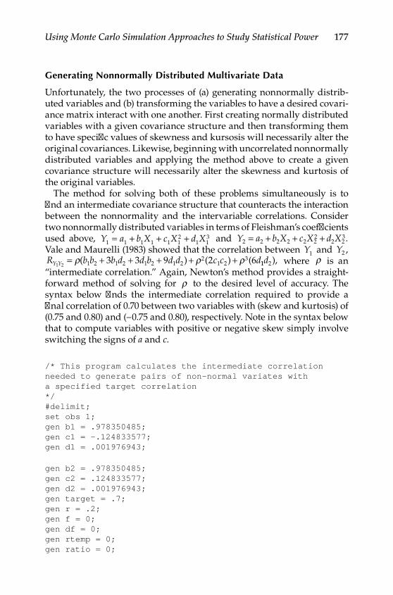
Using Monte Carlo Simulation Approaches to Study Statistical Power 177
generating Nonnormally Distributed Multivariate Data
Unfortunately, the two processes of (a) generating nonnormally distrib‑uted variables and (b) transforming the variables to have a desired covari‑ance matrix interact with one another. First creating normally distributed variables with a given covariance structure and then transforming them to have specific values of skewness and kursosis will necessarily alter the original covariances. Likewise, beginning with uncorrelated nonnormally distributed variables and applying the method above to create a given covariance structure will necessarily alter the skewness and kurtosis of the original variables.
The method for solving both of these problems simultaneously is to find an intermediate covariance structure that counteracts the interaction between the nonnormality and the intervariable correlations. Consider two nonnormally distributed variables in terms of Fleishman’s coefficients used above, Y a b X c X d X1 1 1 1 1 1
21 1
3= + + + and Y a b X c X d X2 2 2 2 2 22
2 23= + + + .
Vale and Maurelli (1983) showed that the correlation between Y1 and Y2 , R b b b d d b d d c c dY Y1 2 1 2 1 2 1 2 1 2
21 2
33 3 9 2 6= + + + + +ρ ρ ρ( ) ( ) ( 11 2d ), where ρ is an “intermediate correlation.” Again, Newton’s method provides a straight‑forward method of solving for ρ to the desired level of accuracy. The syntax below finds the intermediate correlation required to provide a final correlation of 0.70 between two variables with (skew and kurtosis) of (0.75 and 0.80) and (−0.75 and 0.80), respectively. Note in the syntax below that to compute variables with positive or negative skew simply involve switching the signs of a and c.
/* This program calculates the intermediate correlationneeded to generate pairs of non-normal variates witha specified target correlation*/#delimit;set obs 1;gen b1 = .978350485;gen c1 = -.124833577;gen d1 = .001976943;
gen b2 = .978350485;gen c2 = .124833577;gen d2 = .001976943;gen target = .7;gen r = .2;gen f = 0;gen df = 0;gen rtemp = 0;gen ratio = 0;
Y100315.indb 177 7/15/09 3:00:06 PM

178 Statistical Power Analysis with Missing Data
quietly forvalues i=1/50 {;replace f =
(r^3*6*d1*d2+r^2*2*c1*c2+r*(b1*b2+3*b1*d2+3*d1*b2+9*d1*d2)-target);replace df =
(3*r^2*6*d1*d2+2*r^2*c1*c2+(b1*b2+3*b1*d2+3*d1*b2+9*d1*d2));replace ratio = f/df;quietly replace rtemp = r - ratio;quietly replace r = rtemp if abs(rtemp - ratio) > .00001;};tab r;
Another important topic, which we will not consider here, involves generating data from nonnormally distributed latent variables. The general approach, which allows researchers to manipulate the skew‑ness and kurtosis of both latent and manifest variables, was outlined by Mattson (1997). A subsequent Monte Carlo study designed to compare his approach with two alternatives (Burr’s [1942] method and an approach based upon the generalized lambda distribution outlined in Ramberg & Schmeiser [1974]), suggested that Mattson’s approach appeared to per‑form best. Other researchers, such as B. Muthén and Kaplan (1985), have examined the effects of “coarsening” variables, which is another strat‑egy that can be used to generate models with nonnormal data, and of course it is also possible to generate manifest and observed variables based upon nonnormal parametric distributions such as uniform, beta, gamma, or chi‑square.
Evaluating Convergence Rates for a Given Model
Enders and Bandalos (2001) conducted a Monte Carlo study to compare four methods of missing data estimation (full information maximum likelihood, list‑wise deletion, pair‑wise deletion, and hot‑deck imputation). Their study considered a fairly simple three factor model (shown in Figure 9.4) under a wide variety of conditions. Specifically, they considered the effects of factor loadings (.4, .6, or .8), sample size (100, 250, 500, or 750), proportion of cases with missing data (2, 5, 10, 15, or 25%), and type of missing data mechanism (MCAR or MAR) for a total of 120 different conditions.
Each condition was replicated 250 times (requiring a total of 30,000 dif‑ferent data sets and 12 million observations of nine variables apiece, each of which had to be analyzed separately). Based on their analyses, Enders and Bandalos (2001) were interested in four different outcome measures
Y100315.indb 178 7/15/09 3:00:06 PM
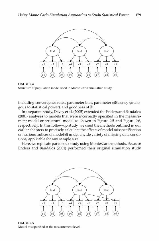
Using Monte Carlo Simulation Approaches to Study Statistical Power 179
including convergence rates, parameter bias, parameter efficiency (analo‑gous to statistical power), and goodness of fit.
In a separate study, Davey et al. (2005) extended the Enders and Bandalos (2001) analyses to models that were incorrectly specified in the measure‑ment model or structural model as shown in Figure 9.5 and Figure 9.6, respectively. In this follow‑up study, we used the methods outlined in our earlier chapters to precisely calculate the effects of model misspecification on various indices of model fit under a wide variety of missing data condi‑tions, applicable for any sample size.
Here, we replicate part of our study using Monte Carlo methods. Because Enders and Bandalos (2001) performed their original simulation study
Eta1
x1
e1
x2
e2
x3
e3
Eta2
x4
e4
x5
e5
x6
e6
Eta3
x7
e7
x8
e8
x9
e9
Figure 9.4Structure of population model used in Monte Carlo simulation study.
Eta1
x1
e1
x2
e2
x3
e3
Eta2
x4
e4
x5
e5
x6
e6
Eta3
x7
e7
x8
e8
x9
e9
Figure 9.5Model misspecified at the measurement level.
Y100315.indb 179 7/15/09 3:00:07 PM

180 Statistical Power Analysis with Missing Data
using AMOS to estimate models and SAS to generate data and calculate results, we follow the same procedure here for a small subset of their orig‑inal conditions, adding a few new conditions of our own. Following the outline from Paxton et al. (2001), we work through the steps of our small simulation study. The AMOS syntax is quite lengthy, and so we provide it in a separate section at the end of this chapter rather than in the text itself.
Step 1: Developing a research Question
Enders and Bandalos (2001) found that full information maximum likeli‑hood estimation worked best under MCAR and MAR missing data con‑ditions for a model which was correctly specified. They also found that convergence rates were low with very small [N = 100] sample sizes. How well does FIML estimation perform for models that are misspecified at either the measurement or structural level?
Step 2: Creating a Valid Model
In addition to the correctly specified model from Enders and Bandalos (Figure 9.4), we also estimated models that were misspecified at either the measurement or structural level, consistent with Davey et al. (2005) as shown in Figure 9.5 and Figure 9.6.
Step 3: Selecting experimental Conditions
For the purposes of this small‑scale simulation study, we focus on the situations that are likely to be most problematic in terms of model estima‑tion. Specifically, we limit our analysis to the situations where data are
Eta1
x1
e1
x2
e2
x3
e3
Eta2
x4
e4
x5
e5
x6
e6
Eta3
x7
e7
x8
e8
x9
e9
Figure 9.6Model misspecified at the structural level.
Y100315.indb 180 7/15/09 3:00:08 PM
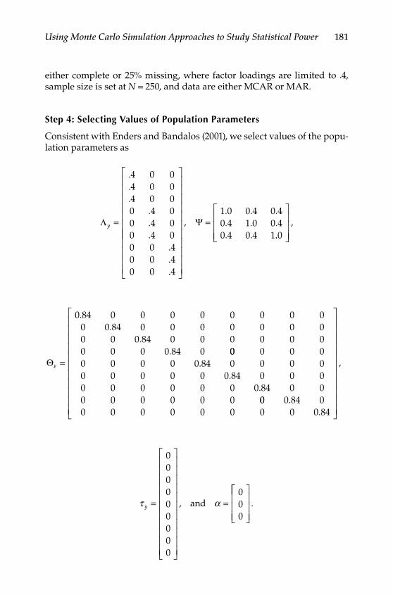
Using Monte Carlo Simulation Approaches to Study Statistical Power 181
either complete or 25% missing, where factor loadings are limited to .4, sample size is set at N = 250, and data are either MCAR or MAR.
Step 4: Selecting Values of Population Parameters
Consistent with Enders and Bandalos (2001), we select values of the popu‑lation parameters as
Λy =
.
.
....
.
.
.
4 0 04 0 04 0 00 4 00 4 00 4 00 0 40 0 40 0 4
=,. . .. . .. .
Ψ1 0 0 4 0 40 4 1 0 0 40 4 0 4 1..
,0
Θε =
0 84 0 0 0 0 0 0 0 00 0 84 0 0 0 0 0 0 00 0 0 84 0 0 0 0 0 00 0 0 0 84 0
..
.. 00 0 0 0
0 0 0 0 0 84 0 0 0 00 0 0 0 0 0 84 0 0 00 0 0 0 0 0 0 84 0 00 0 0 0 0 0
..
.00 0 84 0
0 0 0 0 0 0 0 0 0 84.
.
,
τ αy =
=
000000000
000
, and
.
Y100315.indb 181 7/15/09 3:00:08 PM

182 Statistical Power Analysis with Missing Data
The diagonal elements of Θε are calculated as 1 4 2− (. ) . Matrix multiplica‑tion gives us an implied covariance matrix of
S =
1 000 0 160 0 160 0 064 0 064 0 064 0 064 0 064 0 064. . . . . . . . .00 160 1 000 0 160 0 064 0 064 0 064 0 064 0 064 0 0640
. . . . . . . . .
.. . . . . . . . .
.160 0 160 1 000 0 064 0 064 0 064 0 064 0 064 0 064
0 0064 0 064 0 064 1 000 0 160 0 160 0 064 0 064 0 0640 0
. . . . . . . .. 664 0 064 0 064 0 160 1 000 0 160 0 064 0 064 0 064
0 06. . . . . . . .
. 44 0 064 0 064 0 160 0 160 1 000 0 064 0 064 0 0640 064
. . . . . . . .. 00 064 0 064 0 064 0 064 0 064 1 000 0 160 0 160
0 064 0. . . . . . . .
. .. . . . . . . .
. .064 0 064 0 064 0 064 0 064 0 160 1 000 0 160
0 064 0 0064 0 064 0 064 0 064 0 064 0 160 0 160 1 000. . . . . . .
.
Step 5: Selecting an appropriate Software Package
Following Davey et al. (2005), Stata was used to estimate study data and AMOS was used to estimate the structural equation models. Results were output from AMOS as ASCII text files and analyzed within Stata.
Step 6: Conducting the Simulations
With the small number of conditions included in this sample simulation, the simulations can be run directly. Again, following Enders and Bandalos (2001), because the number of nonconverged replications was of interest, we estimated a fixed number of 250 replications under each condition. If we were interested in running a study with a large number of conditions, it makes the most sense to run a simulation as a series of batch or execut‑able files. AMOS has a very convenient interface with VisualBasic, MPlus has internal simulation structures, and LISREL can easily be run in batch mode. For more complicated simulation studies, it is generally beneficial to invest more time on the programming side, whereas brute force works just fine with a simple simulation such as this one.
Step 7: File Storage
Our study required us to estimate 250 different data sets, each contain‑ing 500 observations (125,000 observations, each with nine variables). The same data sets were then used to estimate models with complete, MCAR, or MAR data for the correct, measurement misspecified, or structurally mis‑specified models. Ordinarily, separate data files would be estimated under each condition, requiring nine times as many observations. However,
Y100315.indb 182 7/15/09 3:00:09 PM

Using Monte Carlo Simulation Approaches to Study Statistical Power 183
the approach we use here reduces the sampling variability — condition becomes two repeated factors — for illustrative purposes. Data sets can be stored as ASCII text, Excel files, or as Microsoft Access database files.
AMOS syntax files, though long compared with what most researchers are accustomed to, do not require much hard drive space because they are stored as ASCII files, as are the Stata syntax files and all output. To avoid clutter, we stored all syntax, data, and output files in separate folders.
Step 8: Troubleshooting and Verification
It is a rare simulation study that runs successfully on the first attempt. As such, we initially wrote our simulation study to include a very small number of replications (one). Once we verified that the output generated by our program matched completely with the output generated by run‑ning the same model manually, we proceeded to add a loop for a small number of replications (usually 3 to 5), followed by another period of veri‑fication. Finally, after running the entire sequence of 250 replications, we compared output for a randomly selected replication manually. Similar checks were made to ensure that the output files were being read correctly prior to tabulating the results.
One final consideration for this small simulation study is that, because the unit of analysis is the replication (i.e., the same data set was analyzed under each of the study conditions), that is the way our data set was ultimately structured. This means that we had to create separate variable names for the model chi‑square values as calculated under each of the different model con‑ditions. In turn, this required the use of a systematic naming convention.
For this study, the first letter of the variable name (most statistical pack‑ages require that variable names begin with letters rather than numbers) indicated which model was being estimated (x = correct, y = structural mis‑specification, z = measurement misspecification), followed by an abbrevi‑ated name for the fit index (e.g., chi = chi‑squared, rms = RMSEA, etc.) and separate numerical codes reflecting each level of the various design factors: missing data type (0 = complete, 1 = MCAR, 2 = MAR), factor loading (1 = .4, 2 = .6, and 3 = .8), sample size (1 = 100, 2 = 250, 3 = 500, 5 = 750), and proportion of cases with missing data (1 = 2%, 2 = 5%, 3 = 10%, 4 = 15%, 5 = 25%). Correct and complete documentation is essential to the successful management of a simulation study. Long (2008) has a number of very useful suggestions for managing most of the workflow tasks associated with a Monte Carlo study and we highly recommend this volume as a useful starting point.
Note that though not all conditions were estimated for this Monte Carlo study, we wrote our syntax in a more general format so that it can easily be extended to do so. Because we were interested in evaluating various fit indices, not all of which are calculated automatically with incomplete
Y100315.indb 183 7/15/09 3:00:09 PM

184 Statistical Power Analysis with Missing Data
data, it was also necessary to estimate both the saturated and indepen‑dence models under each condition.
Step 9: Summarizing the results
One of the first things you will discover when conducting a Monte Carlo study is that it generates a tremendous volume of data, and it is not always easy to summarize these data values. In this simple case, we have three different models (correct, structural misspecification, and measurement misspecification) under three different data conditions (complete, 25% cases with MCAR data, and 25% cases with MAR data). For each of these nine combinations in turn we might be interested in knowing about the convergence rates and then a variety of summary statistics (say the mean, median, and the 5th and 95th percentile values) across several different fit indices (model chi‑square, independence chi‑square, RMSEA, TLI, etc.).
It probably makes the most sense to look at how estimation of each model differs across each type of condition. For that reason, our table of results should probably have condition nested within model. Table 9.2 presents the convergence rates for our small Monte Carlo study. As we can see, not all of our 250 replications in each condition provided proper solutions, even with complete data. Overall, however, convergence rates were high‑est with complete data, followed by MCAR data and lowest when data were MAR. Similarly, estimation of the correct model most often led to a valid solution, followed by the structurally misspecified model and the measurement misspecification providing the lowest convergence rates at just 56% of models. (Under slightly different conditions however, specifi‑cally when factor loadings were higher, nearly all models converged.)
Similarly, we can capture the results from our Monte Carlo study in terms of their effects on various aspects of model fit. Table 9.3 illustrates the model chi‑square statistic, the chi‑square statistic for the indepen‑dence model, the RMSEA, and the Tucker‑Lewis Index (TLI). Because these statistics do not have normal distributions, we focus on the median values along with their 90% confidence interval as represented in the val‑ues of the 5th and 95th percentiles. Using data from this table, Figure 9.7 illustrates, for example, that whereas the median values of the RMSEA are
Table 9.2
Convergence Rates for Monte Carlo Simulation
Converged Analyses (%)
Model Complete MCAR MAR
Correct 228 (91.2) 215 (86.0) 202 (80.8)Structural misspecified 220 (88.0) 205 (82.0) 186 (74.4)Measurement misspecified 177 (70.8) 170 (68.0) 140 (56.0)
Y100315.indb 184 7/15/09 3:00:09 PM
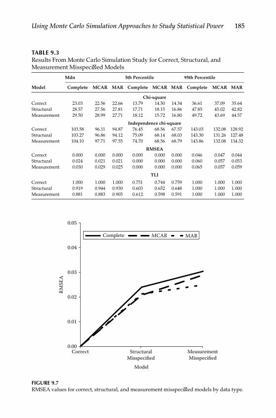
Using Monte Carlo Simulation Approaches to Study Statistical Power 185
0.00
0.01
0.02
0.03
0.04
0.05
StructuralMisspecified
Correct MeasurementMisspecified
Model
RMSE
A
Complete MCAR MAR
Figure 9.7RMSEA values for correct, structural, and measurement misspecified models by data type.
Table 9.3Results From Monte Carlo Simulation Study for Correct, Structural, and Measurement Misspecified Models
Mdn 5th Percentile 95th Percentile
Model Complete MCAR MAR Complete MCAR MAR Complete MCAR MAR
Chi‑squareCorrect 23.03 22.56 22.66 13.79 14.50 14.34 36.61 37.09 35.64Structural 28.57 27.56 27.81 17.71 18.15 16.86 47.85 45.02 42.82Measurement 29.50 28.99 27.71 18.12 15.72 16.80 49.72 43.69 44.57
Independence chi‑squareCorrect 103.58 96.11 94.87 76.45 68.56 67.57 143.03 132.08 128.92Structural 103.27 96.86 94.12 75.09 68.14 68.03 143.30 131.26 127.48Measurement 104.10 97.71 97.55 74.70 68.56 68.79 143.86 132.08 134.32
RMSEACorrect 0.000 0.000 0.000 0.000 0.000 0.000 0.046 0.047 0.044Structural 0.024 0.021 0.021 0.000 0.000 0.000 0.060 0.057 0.053Measurement 0.030 0.029 0.025 0.000 0.000 0.000 0.065 0.057 0.059
TLI
Correct 1.000 1.000 1.000 0.751 0.744 0.759 1.000 1.000 1.000Structural 0.919 0.944 0.930 0.603 0.652 0.648 1.000 1.000 1.000Measurement 0.881 0.883 0.905 0.612 0.598 0.591 1.000 1.000 1.000
Y100315.indb 185 7/15/09 3:00:10 PM
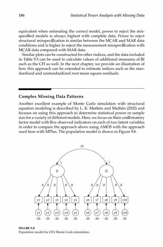
186 Statistical Power Analysis with Missing Data
equivalent when estimating the correct model, power to reject the mis‑specified models is always highest with complete data. Power to reject structural misspecification is similar between the MCAR and MAR data conditions and is higher to reject the measurement misspecification with MCAR data compared with MAR data.
Similar plots can be constructed for other indices, and the data included in Table 9.3 can be used to calculate values of additional measures of fit such as the CFI as well. In the next chapter, we provide an illustration of how this approach can be extended to estimate indices such as the stan‑dardized and unstandardized root mean square residuals.
Complex Missing Data Patterns
Another excellent example of Monte Carlo simulation with structural equation modeling is described by L. K. Muthén and Muthén (2002) and focuses on using this approach to determine statistical power or sample size for a variety of different models. Here, we focus on their confirmatory factor model with five observed indicators on each of two latent variables in order to compare the approach above using AMOS with the approach used here with MPlus. The population model is shown in Figure 9.8.
1
f1
y1
.36
e1
.8
y2
.36
e2
.8
y3
.36
e3
.8
y4
.36
e4
.8
y5
.36
e5
.8
1
f2
y6
.36
e6
y7
.36
e7
y8
.36
e8
y9
.36
e9
y10
.36
e10
.8 .8 .8 .8 .8
.25
Figure 9.8Population model for CFA Monte Carlo simulation.
Y100315.indb 186 7/15/09 3:00:10 PM
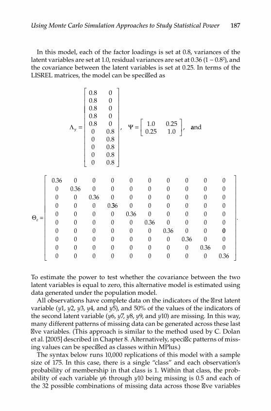
Using Monte Carlo Simulation Approaches to Study Statistical Power 187
In this model, each of the factor loadings is set at 0.8, variances of the latent variables are set at 1.0, residual variances are set at 0.36 (1 − 0.82), and the covariance between the latent variables is set at 0.25. In terms of the LISREL matrices, the model can be specified as
Λy =
0 8 00 8 00 8 00 8 00 8 00 0 80 0 80 0 80 0 80 0 8
.
.
.
.
......
=
, . .
. .,Ψ 1 0 0 25
0 25 1 0aand
Θε =
0 36 0 0 0 0 0 0 0 0 00 0 36 0 0 0 0 0 0 0 00 0 0 36 0 0 0 0 0 0 00 0 0 0
..
..336 0 0 0 0 0 0
0 0 0 0 0 36 0 0 0 0 00 0 0 0 0 0 36 0 0 0 00 0 0 0 0 0 0 36 0 0
..
. 000 0 0 0 0 0 0 0 36 0 00 0 0 0 0 0 0 0 0 36 00 0 0 0 0 0 0 0 0 0 36
..
.
.
To estimate the power to test whether the covariance between the two latent variables is equal to zero, this alternative model is estimated using data generated under the population model.
All observations have complete data on the indicators of the first latent variable (y1, y2, y3, y4, and y5), and 50% of the values of the indicators of the second latent variable (y6, y7, y8, y9, and y10) are missing. In this way, many different patterns of missing data can be generated across these last five variables. (This approach is similar to the method used by C. Dolan et al. [2005] described in Chapter 8. Alternatively, specific patterns of miss‑ing values can be specified as classes within MPlus.)
The syntax below runs 10,000 replications of this model with a sample size of 175. In this case, there is a single “class” and each observation’s probability of membership in that class is 1. Within that class, the prob‑ability of each variable y6 through y10 being missing is 0.5 and each of the 32 possible combinations of missing data across those five variables
Y100315.indb 187 7/15/09 3:00:10 PM

188 Statistical Power Analysis with Missing Data
may be generated (although the one missing on all five variables would be very uncommon). To generate data where 50% of cases were missing on all of y6 through y10, two classes would have to be generated, each with probability of membership equal to 0.5. In the first class, the probability of missing data on y6 through y10 would be 0; in the second class, the prob‑ability of missing data on y6 through y10 would be 1.
TITLE: cfamodel.inp normal, missingMONTECARLO: NAMES ARE y1-y10; NOBSERVATIONS = 175; NREPS = 10000; SEED = 53487; CLASSES = C(1); GENCLASSES = C(1); PATMISS = y6 (.5) y7 (.5) y8 (.5) y9 (.5) y10 (.5); PATPROB = 1; SAVE = cfamodel.sav;ANALYSIS: TYPE = MIXTURE MISSING; ESTIMATOR = ML;MODEL MONTECARLO: %OVERALL% f1 BY y1-y5*.8; f2 BY y6-y10*.8; f1@1 f2@1; y1-y10*.36; f1 WITH f2*.25;MODEL: %OVERALL% f1 BY y1-y5*.8; f2 BY y6-y10*.8; f1@1 f2@1; y1-y10*.36; f1 WITH f2*.25;OUTPUT: PATTERNS TECH9;
Troubleshooting Tip
We strongly recommend that, if you do not have a copy of MPlus, you download the student version of this software and try the syntax above. Use it as a starting point to make further modifications to the patterns of missing data. It is also a good idea to replicate results from earlier sections of this book using the Monte Carlo approach in order to see how closely the results agree in a specific context. Doing so can also help you to gain a better appreciation for the pros and cons of Monte Carlo versus popula‑tion‑based approaches.
Y100315.indb 188 7/15/09 3:00:10 PM

Using Monte Carlo Simulation Approaches to Study Statistical Power 189
Running this syntax generates a bit of output that is not found in the usual analysis. As shown in Table 9.4, MPlus provides information about each pattern of incomplete data in the first replication, which we have reorganized here in terms of each variable which may potentially be miss‑ing. Notice that in this first replication, 31 of 32 possible missing data pat‑terns are represented (only the pattern where y7 and y8 are observed and y6, y9, and y10 are missing does not occur).
Other useful components of the output include the number of successful replications (in this case, all 10,000 were successfully estimated) and infor‑mation about model fit. The output then proceeds to provide information
Table 9.4
Frequencies of Each Missing Data Pattern in First Data Set
y6 y7 y8 y9 y10Number of
Cases
1 1 1 1 1 41 1 1 1 0 71 1 1 0 1 41 1 1 0 0 111 1 0 1 1 51 1 0 1 0 51 1 0 0 1 71 1 0 0 0 41 0 1 1 1 51 0 1 1 0 61 0 1 0 1 41 0 1 0 0 81 0 0 1 1 51 0 0 1 0 61 0 0 0 1 81 0 0 0 0 100 1 1 1 1 50 1 1 1 0 50 1 1 0 1 50 1 0 1 1 90 1 0 1 0 50 1 0 0 1 50 1 0 0 0 60 0 1 1 1 50 0 1 1 0 60 0 1 0 1 50 0 1 0 0 50 0 0 1 1 20 0 0 1 0 20 0 0 0 1 70 0 0 0 0 4
Y100315.indb 189 7/15/09 3:00:11 PM

190 Statistical Power Analysis with Missing Data
about estimates for each of the model parameters, including the covari‑ance between the two latent variables. Along with the estimates, their standard errors, and a 95% confidence interval, MPlus provides informa‑tion about the proportion of replications in which the model parameter was statistically significant, in this case 81.2% for a power of .812. Power for other model parameters can be obtained in the same way; power for other sample sizes may be obtained by rerunning the syntax with dif‑ferent sample sizes. Likewise, power under different assumptions can be obtained by selecting different values for the population parameters, such as covariance of .5 between the latent variables or with different values of the factor loadings. MPlus has facilities for specifying a missingness mechanism in order to generate MAR data as well as for generating non‑normally distributed variables.
Conclusions
Monte Carlo methods represent an extremely important set of tools for power analysis with missing data. Under situations where a specific model or small set of conditions is of interest, Monte Carlo methods may often be the easiest and most efficient way to estimate statistical power. Under other conditions, such as with a large number of missing data patterns, in real‑world situations such as when convergence rates are of primary interest, or when raw data are necessary such as with nonnor‑mally distributed variables, the Monte Carlo approach may be the only practical way to address an applied research question. In this chapter, we have provided a set of tools useful for generating data as well as estimating statistical power with missing data that greatly extend the approaches that have been described in earlier chapters. The primary downsides to Monte Carlo methods are their time and storage intensive nature, as well as the fact that their results are typically only applicable to the specific circumstances under investigation. Estimating power for different sample sizes or for different population parameters generally requires generating completely new data sets and estimating the models of interest on each on. Following the procedures outlined by Paxton and colleagues (2001) is one way to help manage the complexity of conduct‑ing a Monte Carlo study. Additional suggestions relevant to managing a Monte Carlo study can be found in the recent volume by Long (2008) on workflow.
Y100315.indb 190 7/15/09 3:00:11 PM
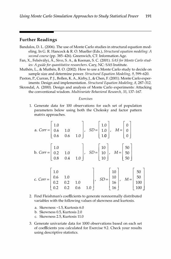
Using Monte Carlo Simulation Approaches to Study Statistical Power 191
Further Readings
Bandalos, D. L. (2006). The use of Monte Carlo studies in structural equation mod‑eling. In G. R. Hancock & R. O. Mueller (Eds.), Structural equation modeling: A second course (pp. 385–426). Greenwich, CT: Information Age.
Fan, X., Felsővályi, Á., Sivo, S. A., & Keenan, S. C. (2001). SAS for Monte Carlo stud‑ies: A guide for quantitative researchers. Cary, NC: SAS Institute.
Muthén, L., & Muthén, B. O. (2002). How to use a Monte Carlo study to decide on sample size and determine power. Structural Equation Modeling, 9, 599–620.
Paxton, P., Curran, P. J., Bollen, K. A., Kirby, J., & Chen, F. (2001). Monte Carlo exper‑iments: Design and implementation. Structural Equation Modeling, 8, 287–312.
Skrondal, A. (2000). Design and analysis of Monte Carlo experiments: Attacking the conventional wisdom. Multivariate Behavioral Research, 35, 137–167.
Exercises
1. Generate data for 100 observations for each set of population parameters below using both the Cholesky and factor pattern matrix approaches.
a. Corr SD=
=1 00 6 1 00 6 0 6 1 0
1 01 01
.
. .
. . .,
.
.
.00
000
=
, M
b. Corr SD=
=
1 00 2 1 00 8 0 4 1 0
101010
.
. .
. . .,
=
, M505050
c.
.
. .
. . .
. . . .
Corr =
1 00 6 1 00 2 0 2 1 00 2 0 2 0 6 1 0
=
=
, ,SD M
10101616
5050
100100
2. Find Fleishman’s coefficients to generate nonnormally distributed variables with the following values of skewness and kurtosis.
a. Skewness −1.5, Kurtosis 6.0b. Skewness 0.5, Kurtosis 2.0c. Skewness 2.5, Kurtosis 11.0
3. Generate univariate data for 1000 observations based on each set of coefficients you calculated for Exercise 9.2. Check your results using descriptive statistics.
Y100315.indb 191 7/15/09 3:00:11 PM

192 Statistical Power Analysis with Missing Data
4. Find the intermediate correlations corresponding to the following pairs of variables.
5. Design a Monte Carlo study with at least three factors in it. Be sure to consider each of the nine steps outlined by Paxton et al. (2000).
6. Replicate the Monte Carlo CFA study using a different seed. How do your results compare? Download the student version of MPlus to do so, if needed.
7. Write syntax to replicate the Monte Carlo CFA study:
a. To determine the power to detect a correlation of .4 using a sample size of 100.
b. To determine the sample size needed to detect a correlation of .25 with a power of .9.
AMOS Syntax Used for Our Simulation Study
Attribute VB_Name = "Module1"Option Explicit
Sub Main() Dim infile As String Dim outfile As String Dim i As Integer Dim dbMain As DAO.Database Dim tblTemp As DAO.TableDef Dim tblName As String Dim strSQL As String Dim strSQLDelete As String Dim it As Integer Dim m As Integer
Set dbMain = OpenDatabase("c:\nm750f80.mdb") tblName = "c:\nm750f80" strSQLDelete = "DROP TABLE Temp" ‘dbMain.Execute (strSQLDelete)
Open "c:\cfr\methods\fiml\xnm750f80_indexes.txt" For Output As #1
Variable 1 Variable 2
Skewness Kurtosis Skewness Kurtosis Correlation
a −1.5 6.0 −1.5 6.0 .5b 2.5 11 2.5 6.0 .7c 2.5 11 −2.5 6.0 .7
Y100315.indb 192 7/15/09 3:00:12 PM

Using Monte Carlo Simulation Approaches to Study Statistical Power 193
Open "c:\cfr\methods\fiml\xnm750f80_satcov.txt" For Output As #2 Open "c:\cfr\methods\fiml\xnm750f80_matrices.txt" For Output As #3
For m = 1 To 5 For it = 1 To 250 strSQL = "SELECT * INTO Temp FROM nm750f80 WHERE IT = " & it & " and M = " & m
'create Temp table and drop extra fields dbMain.Execute (strSQL) dbMain.Execute ("alter table Temp drop column it") dbMain.Execute ("alter table Temp drop column m") dbMain.Execute ("alter table Temp drop column s") dbMain.Execute ("alter table Temp drop column loading")
Call FitAmosModel(m, it) 'remove Temp table strSQLDelete = "DROP TABLE Temp" dbMain.Execute (strSQLDelete)
Next it Next m Close #1 Close #2 Close #3 dbMain.CloseEnd Sub
Sub FitAmosModel(m, it) 'Attach Amos data file Dim ObsVars As Variant Dim ModelAdmissible As Boolean, ModelConverged As Boolean Dim SaturatedAdmissible As Boolean, SaturatedConverged As Boolean Dim IndepConverged As Boolean, IndepAdmissible As Boolean, IndepCmin As Double, IndepNparms As Integer Dim ModelCmin As Double, SaturatedCmin As Double, P As Double Dim Chi2 As Double Dim ModelNparms As Integer, SaturatedNparms As Integer, Df As Integer, N As Integer
ObsVars = Array("x1", "x2", "x3", "x4", "x5", "x6", "x7", "x8", "x9")
Y100315.indb 193 7/15/09 3:00:12 PM

194 Statistical Power Analysis with Missing Data
Call FitSaturated(ObsVars, SaturatedConverged, SaturatedAdmissible, SaturatedCmin, SaturatedNparms, m, it)
Call FitIndependent(ObsVars, IndepConverged, IndepAdmissible, IndepCmin, IndepNparms)
Dim Sem As New AmosEngine Sem.TextOutput Sem.Standardized Sem.Smc ‘Sem.AllImpliedMoments Sem.ModelMeansAndIntercepts Sem.Iterations (1000)
'Model specification starts here Sem.BeginGroup "c:\nm750f80.mdb", "Temp" Sem.Structure "f1 (load1)" Sem.Structure "f2 (load2)" Sem.Structure "f3 (load3)" Sem.Structure "x1 = (xbar1) + (1) f1 + (1) e1" Sem.Structure "x2 = (xbar2) + (load4) f1 + (1) e2" Sem.Structure "x3 = (xbar3) + (load5) f2 + (1) e3" Sem.Structure "x4 = (xbar4) + (1) f2 + (1) e4" Sem.Structure "x5 = (xbar5) + (load6) f2 + (1) e5" Sem.Structure "x6 = (xbar6) + (load7) f2 + (1) e6" Sem.Structure "x7 = (xbar7) + (1) f3 + (1) e7" Sem.Structure "x8 = (xbar8) + (load8) f3 + (1) e8" Sem.Structure "x9 = (xbar9) + (load9) f3 + (1) e9" Sem.Structure "e1 (e1)" Sem.Structure "e2 (e2)" Sem.Structure "e3 (e3)" Sem.Structure "e4 (e4)" Sem.Structure "e5 (e5)" Sem.Structure "e6 (e6)" Sem.Structure "e7 (e7)" Sem.Structure "e8 (e8)" Sem.Structure "e9 (e9)" Sem.Structure "f1<>f2 (cov1)" Sem.Structure "f2<>f3 (cov2)" Sem.Structure "f1<>f3 (cov3)"
Dim load1 As Double Dim load2 As Double Dim load3 As Double Dim load4 As Double Dim load5 As Double Dim load6 As Double Dim load7 As Double
Y100315.indb 194 7/15/09 3:00:12 PM
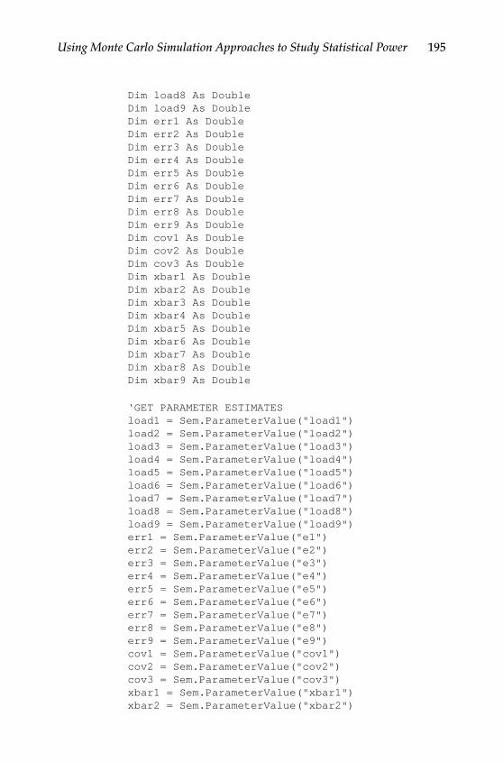
Using Monte Carlo Simulation Approaches to Study Statistical Power 195
Dim load8 As Double Dim load9 As Double Dim err1 As Double Dim err2 As Double Dim err3 As Double Dim err4 As Double Dim err5 As Double Dim err6 As Double Dim err7 As Double Dim err8 As Double Dim err9 As Double Dim cov1 As Double Dim cov2 As Double Dim cov3 As Double Dim xbar1 As Double Dim xbar2 As Double Dim xbar3 As Double Dim xbar4 As Double Dim xbar5 As Double Dim xbar6 As Double Dim xbar7 As Double Dim xbar8 As Double Dim xbar9 As Double
‘GET PARAMETER ESTIMATES load1 = Sem.ParameterValue("load1") load2 = Sem.ParameterValue("load2") load3 = Sem.ParameterValue("load3") load4 = Sem.ParameterValue("load4") load5 = Sem.ParameterValue("load5") load6 = Sem.ParameterValue("load6") load7 = Sem.ParameterValue("load7") load8 = Sem.ParameterValue("load8") load9 = Sem.ParameterValue("load9") err1 = Sem.ParameterValue("e1") err2 = Sem.ParameterValue("e2") err3 = Sem.ParameterValue("e3") err4 = Sem.ParameterValue("e4") err5 = Sem.ParameterValue("e5") err6 = Sem.ParameterValue("e6") err7 = Sem.ParameterValue("e7") err8 = Sem.ParameterValue("e8") err9 = Sem.ParameterValue("e9") cov1 = Sem.ParameterValue("cov1") cov2 = Sem.ParameterValue("cov2") cov3 = Sem.ParameterValue("cov3") xbar1 = Sem.ParameterValue("xbar1") xbar2 = Sem.ParameterValue("xbar2")
Y100315.indb 195 7/15/09 3:00:12 PM

196 Statistical Power Analysis with Missing Data
xbar3 = Sem.ParameterValue("xbar3") xbar4 = Sem.ParameterValue("xbar4") xbar5 = Sem.ParameterValue("xbar5") xbar6 = Sem.ParameterValue("xbar6") xbar7 = Sem.ParameterValue("xbar7") xbar8 = Sem.ParameterValue("xbar8") xbar9 = Sem.ParameterValue("xbar9")
Fit the model 'Extract parameter estimates and admissibility status On Error GoTo 0 ' Turn off error trapping. On Error Resume Next ' Defer error trapping.
ModelConverged = (Sem.FitModel = 0) ModelAdmissible = Sem.Admissible ModelCmin = Sem.Cmin ModelNparms = Sem.npar N = Sem.DataFileNCases Set Sem = Nothing 'Terminate AmosEngine objects DoEvents 'Let system unload AmosEngine objects before continuing Debug.Print "mc: "; ModelConverged Debug.Print "ma: "; ModelAdmissible Debug.Print "sc: "; SaturatedConverged Debug.Print "sa: "; SaturatedAdmissible Debug.Print "ic: "; IndepConverged Debug.Print "ia: "; IndepAdmissible
'recover parameters from the saturated models If (ModelConverged And ModelAdmissible And SaturatedConverged And SaturatedAdmissible And IndepConverged And IndepAdmissible And (ModelNparms <> -1)) Then Chi2 = ModelCmin - SaturatedCmin Df = SaturatedNparms - ModelNparms Dim FitTest As New AmosEngine P = FitTest.ChiSquareProbability(Chi2, CDbl(Df)) FitTest.Shutdown 'Suppresses benign error message
Dim IndepChi As Double Dim IndepDf As Double Dim Prob As Double Dim NFI As Double Dim TLI As Double Dim Rmsea As Double
Y100315.indb 196 7/15/09 3:00:12 PM

Using Monte Carlo Simulation Approaches to Study Statistical Power 197
'CALCULATE FIT INDICES IndepChi = IndepCmin - SaturatedCmin IndepDf = SaturatedNparms - IndepNparms NFI = 1 - (Chi2 / IndepChi) TLI = ((IndepChi / IndepDf) - (Chi2 / Df)) / ((IndepChi / IndepDf) - 1) If Chi2 > Df Then Rmsea = Sqr((Chi2 - Df) / (N * Df)) End If If Chi2 <= Df Then Rmsea = 0 End If
'TESTING Debug.Print "SaturatedCmin: "; Format$(SaturatedCmin, "0.00") Debug.Print "IndepChi: "; Format$(IndepChi, "0.00") Debug.Print "IndepDf: "; Format$(IndepDf, "0.00") Debug.Print " " Debug.Print "Fit of factor model:" Debug.Print "Chi Square: "; Format$(Chi2, "0.00") Debug.Print "Df: "; Df Debug.Print "P: "; Format$(P, "0.00") Debug.Print " " Debug.Print "NFI: "; Format$(NFI, "0.00") Debug.Print "TLI: "; Format$(TLI, "0.00") Debug.Print "RMSEA: "; Format$(Rmsea, "0.00")
'write out the model fit indexes for further analyses Write #1, Round(Chi2, 5), Df, Round(IndepChi, 5), IndepDf, Round(NFI, 5), Round(TLI, 5), Round(Rmsea, 5), m, it Write #3, Round(load1, 5),Round(load2, 5), Round(load3, 5), Round(load4, 5), Round(load5, 5), Round(load6, 5), _ Round(load7, 5),Round(load8, 5), Round(load9, 5), Round(err1, 5), Round(err2, 5), Round(err3, 5), _ Round(err4, 5),Round(err5, 5), Round(err6, 5), Round(err7, 5),Round(err8, 5), Round(err9, 5), _
Y100315.indb 197 7/15/09 3:00:12 PM

198 Statistical Power Analysis with Missing Data
Round(xbar1, 5), Round(xbar2, 5), Round(xbar3, 5), Round(xbar4, 5), Round(xbar5, 5), Round(xbar6, 5), _ Round(xbar7, 5), Round(xbar8, 5), Round(xbar9, 5), Round(cov1, 5), Round(cov2, 5), Round(cov3, 5), _ m, it Set FitTest = Nothing DoEvents Else 'Debug.Print "Sorry, one or both models did not converge to an admissible solution." Write #1, -9, -9, -9, -9, -9, -9, -9, m, it Write #3, -9, -9, -9, -9, -9, -9, _ -9, -9, -9, -9, -9, -9, _ -9, -9, -9, -9, -9, -9, _ -9, -9, -9, -9, -9, -9, _ -9, -9, -9, -9, -9, -9, _ m, it End IfEnd Sub Sub FitSaturated(VarName, Converged, Admissible, Cmin, Nparms, m, it) Dim FirstVar As Integer, LastVar As Integer, ivar As Integer Dim Saturated As New AmosEngine FirstVar = LBound(VarName) LastVar = UBound(VarName) 'saturated models parameters Dim cov11 As Double Dim cov21 As Double Dim cov31 As Double Dim cov41 As Double Dim cov51 As Double Dim cov61 As Double Dim cov71 As Double Dim cov81 As Double Dim cov91 As Double Dim cov22 As Double Dim cov32 As Double Dim cov42 As Double Dim cov52 As Double Dim cov62 As Double Dim cov72 As Double Dim cov82 As Double Dim cov92 As Double Dim cov33 As Double Dim cov43 As Double Dim cov53 As Double
Y100315.indb 198 7/15/09 3:00:12 PM

Using Monte Carlo Simulation Approaches to Study Statistical Power 199
Dim cov63 As Double Dim cov73 As Double Dim cov83 As Double Dim cov93 As Double Dim cov44 As Double Dim cov54 As Double Dim cov64 As Double Dim cov74 As Double Dim cov84 As Double Dim cov94 As Double Dim cov55 As Double Dim cov65 As Double Dim cov75 As Double Dim cov85 As Double Dim cov95 As Double Dim cov66 As Double Dim cov76 As Double Dim cov86 As Double Dim cov96 As Double Dim cov77 As Double Dim cov87 As Double Dim cov97 As Double Dim cov88 As Double Dim cov98 As Double Dim cov99 As Double Dim xbar1 As Double Dim xbar2 As Double Dim xbar3 As Double Dim xbar4 As Double Dim xbar5 As Double Dim xbar6 As Double Dim xbar7 As Double Dim xbar8 As Double Dim xbar9 As Double
With Saturated .ModelMeansAndIntercepts .BeginGroup "c:\nm750f80.mdb", "Temp" .Iterations (1000) .Structure "x1 = (xbar1)" .Structure "x2 = (xbar2)" .Structure "x3 = (xbar3)" .Structure "x4 = (xbar4)" .Structure "x5 = (xbar5)" .Structure "x6 = (xbar6)" .Structure "x7 = (xbar7)" .Structure "x8 = (xbar8)" .Structure "x9 = (xbar9)"
Y100315.indb 199 7/15/09 3:00:12 PM
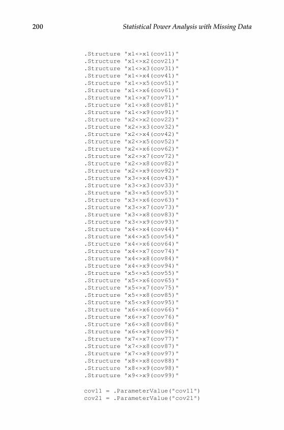
200 Statistical Power Analysis with Missing Data
.Structure "x1<>x1(cov11)" .Structure "x1<>x2(cov21)" .Structure "x1<>x3(cov31)" .Structure "x1<>x4(cov41)" .Structure "x1<>x5(cov51)" .Structure "x1<>x6(cov61)" .Structure "x1<>x7(cov71)" .Structure "x1<>x8(cov81)" .Structure "x1<>x9(cov91)" .Structure "x2<>x2(cov22)" .Structure "x2<>x3(cov32)" .Structure "x2<>x4(cov42)" .Structure "x2<>x5(cov52)" .Structure "x2<>x6(cov62)" .Structure "x2<>x7(cov72)" .Structure "x2<>x8(cov82)" .Structure "x2<>x9(cov92)" .Structure "x3<>x4(cov43)" .Structure "x3<>x3(cov33)" .Structure "x3<>x5(cov53)" .Structure "x3<>x6(cov63)" .Structure "x3<>x7(cov73)" .Structure "x3<>x8(cov83)" .Structure "x3<>x9(cov93)" .Structure "x4<>x4(cov44)" .Structure "x4<>x5(cov54)" .Structure "x4<>x6(cov64)" .Structure "x4<>x7(cov74)" .Structure "x4<>x8(cov84)" .Structure "x4<>x9(cov94)" .Structure "x5<>x5(cov55)" .Structure "x5<>x6(cov65)" .Structure "x5<>x7(cov75)" .Structure "x5<>x8(cov85)" .Structure "x5<>x9(cov95)" .Structure "x6<>x6(cov66)" .Structure "x6<>x7(cov76)" .Structure "x6<>x8(cov86)" .Structure "x6<>x9(cov96)" .Structure "x7<>x7(cov77)" .Structure "x7<>x8(cov87)" .Structure "x7<>x9(cov97)" .Structure "x8<>x8(cov88)" .Structure "x8<>x9(cov98)" .Structure "x9<>x9(cov99)"
cov11 = .ParameterValue("cov11") cov21 = .ParameterValue("cov21")
Y100315.indb 200 7/15/09 3:00:12 PM
Using Monte Carlo Simulation Approaches to Study Statistical Power 201
cov31 = .ParameterValue("cov31") cov41 = .ParameterValue("cov41") cov51 = .ParameterValue("cov51") cov61 = .ParameterValue("cov61") cov71 = .ParameterValue("cov71") cov81 = .ParameterValue("cov81") cov91 = .ParameterValue("cov91") cov22 = .ParameterValue("cov22") cov32 = .ParameterValue("cov32") cov42 = .ParameterValue("cov42") cov52 = .ParameterValue("cov52") cov62 = .ParameterValue("cov62") cov72 = .ParameterValue("cov72") cov82 = .ParameterValue("cov82") cov92 = .ParameterValue("cov92") cov33 = .ParameterValue("cov33") cov43 = .ParameterValue("cov43") cov53 = .ParameterValue("cov53") cov63 = .ParameterValue("cov63") cov73 = .ParameterValue("cov73") cov83 = .ParameterValue("cov83") cov93 = .ParameterValue("cov93") cov44 = .ParameterValue("cov44") cov54 = .ParameterValue("cov54") cov64 = .ParameterValue("cov64") cov74 = .ParameterValue("cov74") cov84 = .ParameterValue("cov84") cov94 = .ParameterValue("cov94") cov55 = .ParameterValue("cov55") cov65 = .ParameterValue("cov65") cov75 = .ParameterValue("cov75") cov85 = .ParameterValue("cov85") cov95 = .ParameterValue("cov95") cov66 = .ParameterValue("cov66") cov76 = .ParameterValue("cov76") cov86 = .ParameterValue("cov86") cov96 = .ParameterValue("cov96") cov77 = .ParameterValue("cov77") cov87 = .ParameterValue("cov87") cov97 = .ParameterValue("cov97") cov88 = .ParameterValue("cov88") cov98 = .ParameterValue("cov98") cov99 = .ParameterValue("cov99") xbar1 = .ParameterValue("xbar1") xbar2 = .ParameterValue("xbar2") xbar3 = .ParameterValue("xbar3") xbar4 = .ParameterValue("xbar4") xbar5 = .ParameterValue("xbar5")
Y100315.indb 201 7/15/09 3:00:12 PM

202 Statistical Power Analysis with Missing Data
xbar6 = .ParameterValue("xbar6") xbar7 = .ParameterValue("xbar7") xbar8 = .ParameterValue("xbar8") xbar9 = .ParameterValue("xbar9")
On Error GoTo 0 ' Turn off error trapping. On Error Resume Next ' Defer error trapping. Converged = (.FitModel = 0) Admissible = .Admissible Cmin = .Cmin Nparms = .npar If (Converged And Admissible) Then 'write out the model fit indexes for further analyses Write #2, Round(cov11, 5), Round(cov21, 5), Round(cov31, 5), Round(cov41, 5), Round(cov51, 5), Round(cov61, 5), _ Round(cov71, 5), Round(cov81, 5), Round(cov91, 5), Round(cov22, 5), Round(cov32, 5), Round(cov42, 5), _ Round(cov52, 5), Round(cov62, 5), Round(cov72, 5), Round(cov82, 5), Round(cov92, 5), Round(cov33, 5), _ Round(cov43, 5), Round(cov53, 5), Round(cov63, 5), Round(cov73, 5), Round(cov83, 5), Round(cov93, 5), _ Round(cov44, 5), Round(cov54, 5), Round(cov64, 5), Round(cov74, 5), Round(cov84, 5), Round(cov94, 5), _ Round(cov55, 5), Round(cov65, 5), Round(cov75, 5), Round(cov85, 5), Round(cov95, 5), Round(cov66, 5), _ Round(cov76, 5), Round(cov86, 5), Round(cov96, 5), Round(cov77, 5), Round(cov87, 5), Round(cov97, 5), _ Round(cov88, 5), Round(cov98, 5), Round(cov99, 5), Round(xbar1, 5), Round(xbar2, 5), Round(xbar3, 5), _ Round(xbar4, 5), Round(xbar5, 5), Round(xbar6, 5), Round(xbar7, 5), Round(xbar8, 5), Round(xbar9, 5), _
m, it Else Write #2, -9, -9, -9, -9, -9, -9, _ -9, -9, -9, -9, -9, -9, _ -9, -9, -9, -9, -9, -9, _ -9, -9, -9, -9, -9, -9, _
Y100315.indb 202 7/15/09 3:00:12 PM
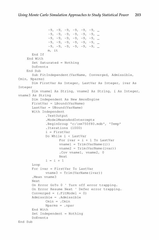
Using Monte Carlo Simulation Approaches to Study Statistical Power 203
-9, -9, -9, -9, -9, -9, _ -9, -9, -9, -9, -9, -9, _ -9, -9, -9, -9, -9, -9, _ -9, -9, -9, -9, -9, -9, _ -9, -9, -9, -9, -9, -9, _ m, it End If End With Set Saturated = Nothing DoEvents End Sub Sub FitIndependent(VarName, Converged, Admissible, Cmin, Nparms) Dim FirstVar As Integer, LastVar As Integer, ivar As Integer Dim vname1 As String, vname2 As String, i As Integer, vname3 As String Dim Independent As New AmosEngine FirstVar = LBound(VarName) LastVar = UBound(VarName) With Independent .TextOutput .ModelMeansAndIntercepts .BeginGroup "c:\nm750f80.mdb", "Temp" .Iterations (1000) i = FirstVar Do While i < LastVar For ivar = i + 1 To LastVar vname1 = Trim(VarName(i)) vname2 = Trim(VarName(ivar)) .Cov vname1, vname2, 0 Next i = i + 1 Loop For ivar = FirstVar To LastVar vname3 = Trim(VarName(ivar)) .Mean vname3 Next On Error GoTo 0 ' Turn off error trapping. On Error Resume Next ' Defer error trapping. Converged = (.FitModel = 0) Admissible = .Admissible Cmin = .Cmin Nparms = .npar End With Set Independent = Nothing DoEventsEnd Sub
Y100315.indb 203 7/15/09 3:00:12 PM

Y100315.indb 204 7/15/09 3:00:12 PM

IIISection
Extensions
Y100315.indb 205 7/15/09 3:00:12 PM

Y100315.indb 206 7/15/09 3:00:12 PM

207
10Additional Issues With Missing Data in Structural Equation Models
In this chapter, we consider several important issues relevant to statistical power which arise in structural equation modeling with missing data. As we mentioned in Chapter 2, one of the most important and challenging aspects of structural equation modeling has to do with evaluation of model fit. To this point, we have generally considered only effects of missing data on statistical power according to the model chi‑square statistic and noncen‑trality parameter. However, power is also an important consideration with regard to other fit indices, many of which are also affected by missing data.
We first illustrate the effects of missing data on a variety of commonly used fit indices. Next, we consider two ways to moderate the effects of missing data on loss of statistical power, focusing on scale reliability and the inclusion of auxiliary variables, both of which are at least partially under the researcher’s control. Careful planning of a study to take advan‑tage of these issues can offer considerable protection against effects of incomplete data.
Effects of Missing Data on Model Fit
There is a growing body of literature to suggest that many commonly used fit indices are affected by the nature and extent of missing data. The paper by Davey et al. (2005) described in Chapter 9 considered the effects of missing data on models that were misspecified in either the structural or measurement model. In addition to the model chi‑square, these authors also considered the effects of missing data on a variety of model fit indi‑ces including the chi‑square, RMSEA, NFI, TLI, CFI, gamma‑hat, and McDonald’s Centrality Index (McDonald, 1989). Effects of missing data varied as a function of the nature of the misspecification, as well as the extent of missing data and whether the data were MCAR or MAR. Much of the influence of missing data on these indices can be traced back to the lower statistical power to reject the independence model with missing
Y100315.indb 207 7/15/09 3:00:12 PM
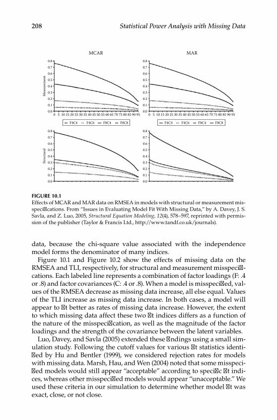
208 Statistical Power Analysis with Missing Data
data, because the chi‑square value associated with the independence model forms the denominator of many indices.
Figure 10.1 and Figure 10.2 show the effects of missing data on the RMSEA and TLI, respectively, for structural and measurement misspecifi‑cations. Each labeled line represents a combination of factor loadings (F: .4 or .8) and factor covariances (C: .4 or .8). When a model is misspecified, val‑ues of the RMSEA decrease as missing data increase, all else equal. Values of the TLI increase as missing data increase. In both cases, a model will appear to fit better as rates of missing data increase. However, the extent to which missing data affect these two fit indices differs as a function of the nature of the misspecification, as well as the magnitude of the factor loadings and the strength of the covariance between the latent variables.
Luo, Davey, and Savla (2005) extended these findings using a small sim‑ulation study. Following the cutoff values for various fit statistics identi‑fied by Hu and Bentler (1999), we considered rejection rates for models with missing data. Marsh, Hau, and Wen (2004) noted that some misspeci‑fied models would still appear “acceptable” according to specific fit indi‑ces, whereas other misspecified models would appear “unacceptable.” We used these criteria in our simulation to determine whether model fit was exact, close, or not close.
0.8
0.7
0.6
0.5
0.4
Mea
sure
men
tSt
ruct
ural
0.3
0.2
0.1
0.00 5 10 15 20 25
MCAR MAR
30 35 40 45 50 55 60 65 70 75 80 85 90 95
F4C4 F4C6 F8C4 F8C8
0.8
0.7
0.6
0.5
0.4
0.3
0.2
0.1
0.00 5 10 15 20 25 30 35 40 45 50 55 60 65 70 75 80 85 90 95
F4C4 F4C6 F8C4 F8C8
0.8
0.7
0.6
0.5
0.4
0.3
0.2
0.1
0.0
0.8
0.7
0.6
0.5
0.4
0.3
0.2
0.1
0.0
Figure 10.1Effects of MCAR and MAR data on RMSEA in models with structural or measurement mis‑specifications. From “Issues in Evaluating Model Fit With Missing Data,” by A. Davey, J. S. Savla, and Z. Luo, 2005, Structural Equation Modeling, 12(4), 578–597, reprinted with permis‑sion of the publisher (Taylor & Francis Ltd., http://www.tandf.co.uk/journals).
Y100315.indb 208 7/15/09 3:00:13 PM
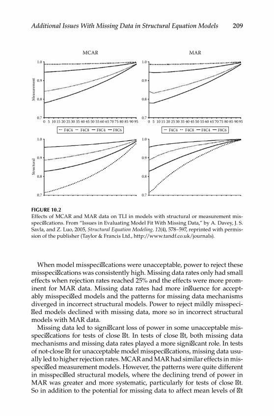
Additional Issues With Missing Data in Structural Equation Models 209
When model misspecifications were unacceptable, power to reject these misspecifications was consistently high. Missing data rates only had small effects when rejection rates reached 25% and the effects were more prom‑inent for MAR data. Missing data rates had more influence for accept‑ably misspecified models and the patterns for missing data mechanisms diverged in incorrect structural models. Power to reject mildly misspeci‑fied models declined with missing data, more so in incorrect structural models with MAR data.
Missing data led to significant loss of power in some unacceptable mis‑specifications for tests of close fit. In tests of close fit, both missing data mechanisms and missing data rates played a more significant role. In tests of not‑close fit for unacceptable model misspecifications, missing data usu‑ally led to higher rejection rates. MCAR and MAR had similar effects in mis‑specified measurement models. However, the patterns were quite different in misspecified structural models, where the declining trend of power in MAR was greater and more systematic, particularly for tests of close fit. So in addition to the potential for missing data to affect mean levels of fit
1.0
MCAR
0.9
Mea
sure
men
t
0.8
0.70 5 10 15 20 25 30 35 40 45 50 55 60 65 70 75 80 85 90 95
F4C4 F4C8 F8C4 F8C6
1.0
MAR
0.9
0.8
0.70 5 10 15 20 25 30 35 40 45 50 55 60 65 70 75 80 85 90 95
F4C4 F4C8 F8C4 F8C6
1.0
0.9
Stru
ctur
al
0.8
0.7
1.0
0.9
0.8
0.7
Figure 10.2Effects of MCAR and MAR data on TLI in models with structural or measurement mis‑specifications. From “Issues in Evaluating Model Fit With Missing Data,” by A. Davey, J. S. Savla, and Z. Luo, 2005, Structural Equation Modeling, 12(4), 578–597, reprinted with permis‑sion of the publisher (Taylor & Francis Ltd., http://www.tandf.co.uk/journals).
Y100315.indb 209 7/15/09 3:00:14 PM
210 Statistical Power Analysis with Missing Data
indices in misspecified models, there are also implications for model accep‑tance/rejection rates, making this an area worthy of further study.
It is also possible to use the output from a simulation study such as this one to construct additional fit indices that are not provided by most struc‑tural equation modeling software programs when there are missing data, such as the standardized or unstandardized root mean square residual (Davey, Savla, & Luo, 2005). Whereas the overall model fit is evaluated in terms of ( )S − Σ , a comparison can also be made on an element‑by‑element basis. To construct this index, the individual elements of S (estimated sample moments) are estimated from the saturated model. The elements of Σ (implied sample moments) are generated from the parameter esti‑mates of the model being estimated. Mathematically, it is calculated as
RMR s p pi
p
j
j i
ij ij= ∑ ∑ − += =
≤
1 1
2 1( ) / ( )σ where p is the number of observed variables.
The unstandardized RMR is calculated from the estimated and implied covariance matrices and the standardized (SRMR) value is calculated from the estimated and implied correlation matrices, ignoring the diagonal ele‑ments, which must always be zero; i.e., the denominator is p p( ).− 1 Smaller values indicate better model fit. The RMR (and SRMR) are also affected by the type and extent of missing data. Values are higher when estimating a correct model when factor loadings and sample sizes are smaller.
For the misspecified measurement model, SRMR values were higher than complete data with MAR data and higher still with MCAR data. The order‑ing of MAR and MCAR data was reversed, however, with the structural misspecification. In each case, the discrepancy in RMR values increases as the proportion of missing data increase and are most pronounced with smaller sample sizes. In other words, the bias in the RMR works in the opposite direction to the model chi‑square. Sample syntax to calculate the RMR is provided in the Appendix but is too lengthy to include here.
There are several potential ways to resolve issues relating to missing data and model fit. One way, specified in Davey et al. (2005), is to estimate the model of interest and independence model using the EM‑generated covariance matrix. LISREL provides this automatically at the start of the output when the FIML option is specified. In LISREL, AMOS, or MPlus, it can also be obtained by requesting the implied covariance matrix. Fit indices generated from this matrix would approximate what their val‑ues would have been in the complete data case. Another possibility is to report the value of a fit index obtained, along with a bootstrapped confi‑dence interval around the value. Ultimately, however, there is simply less power to reject a misspecified model with incomplete data, but the extent to which this is the case can be quite variable depending on factors such as the nature and extent of missing data and the nature and extent of
Y100315.indb 210 7/15/09 3:00:14 PM
Additional Issues With Missing Data in Structural Equation Models 211
the model misspecification. The next section considers how to evaluate this discrepancy at the population level.
Using the NCP to Estimate Power for a Given Index
Kim (2005) showed an important way that the methods described in this book can be extended to a variety of noncentrality based fit indices. By obtaining the minimum value of the fit function for both an alternative model λA and an independence model λB, for example, the CFI, which was discussed in Chapter 2, can easily be calculated for any sample size as CFI N
NAB
= − −−1 1
1( )( ) .λ
λ In this way, it is possible to solve for a sample size thatwill provide a CFI value that is above or below a desired cutoff value. Because the RMSEA is also a noncentrality based index, these methods also apply to the methods of MacCallum and colleagues (1996, 2006) discussed in Chapter 4 for evaluating close, not‑close, and exact fit.
Moderators of Loss of Statistical Power With Missing Data
In Chapter 8, we examined how the design of a study with missing data can affect statistical power by focusing on the specific patterns of data that were observed or unobserved and the proportion of cases observed in each pattern. In this section, we consider two more variables that can help reduce the effects of missing data on the loss of statistical power, both of which are at least partially under the researcher’s control. The first is reliability of the indicators in a study, and the second is the inclusion of an auxiliary variable.
reliability
Interest in increasing the power to detect a treatment effect by increas‑ing the reliability of a dependent variable spans at least four decades (see Cleary & Linn, 1969; Fleiss, 1976; Humphreys & Drasgow, 1989; Nicewander & Price, 1978; Overall, 1989; Overall & Woodard, 1975; Sutcliffe, 1980). The extent to which reliability increases statistical power largely depends on how much it decreases the error variance. Maxwell and his colleagues (1991) noted that ANCOVA models had greater power with more reli‑able indicators. On the other hand, in the presence of marginal reliability ANOVA models with larger gaps between the two measurement points
Y100315.indb 211 7/15/09 3:00:15 PM
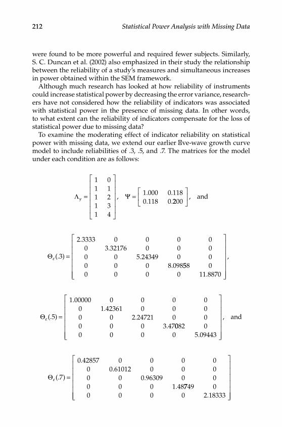
212 Statistical Power Analysis with Missing Data
were found to be more powerful and required fewer subjects. Similarly, S. C. Duncan et al. (2002) also emphasized in their study the relationship between the reliability of a study’s measures and simultaneous increases in power obtained within the SEM framework.
Although much research has looked at how reliability of instruments could increase statistical power by decreasing the error variance, research‑ers have not considered how the reliability of indicators was associated with statistical power in the presence of missing data. In other words, to what extent can the reliability of indicators compensate for the loss of statistical power due to missing data?
To examine the moderating effect of indicator reliability on statistical power with missing data, we extend our earlier five‑wave growth curve model to include reliabilities of .3, .5, and .7. The matrices for the model under each condition are as follows:
Λ Ψy =
=
1 01 11 21 31 4
1 000 0 1180 118 0
, . .. .2200
, and
Θε (. )
..
..
3
2 3333 0 0 0 00 3 32176 0 0 00 0 5 24349 0 00 0 0 8 098
=558 0
0 0 0 0 11 8870.
,
Θε (. )
..
..
5
1 00000 0 0 0 00 1 42361 0 0 00 0 2 24721 0 00 0 0 3 47
=0082 0
0 0 0 0 5 09443.
,
and
Θε (. )
..
..
7
0 42857 0 0 0 00 0 61012 0 0 00 0 0 96309 0 00 0 0 1 48
=7749 0
0 0 0 0 2 18333.
Y100315.indb 212 7/15/09 3:00:16 PM
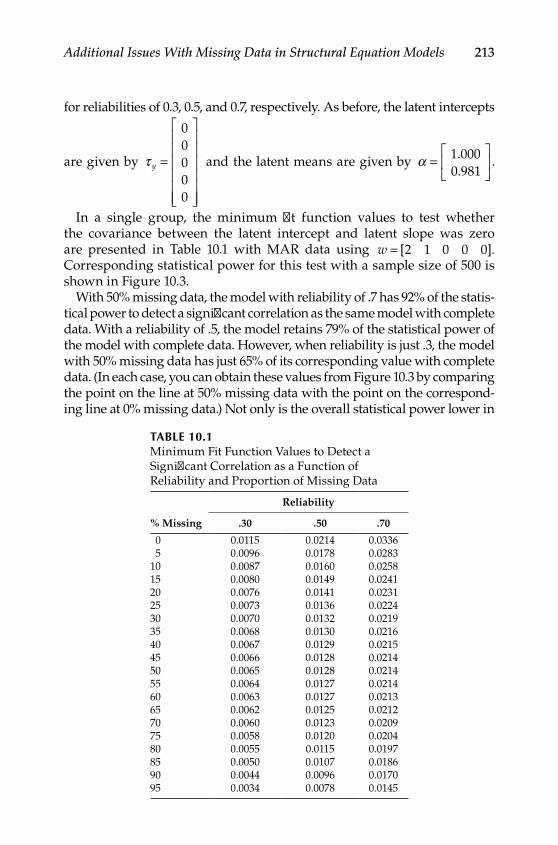
Additional Issues With Missing Data in Structural Equation Models 213
for reliabilities of 0.3, 0.5, and 0.7, respectively. As before, the latent intercepts
are given by τ y =
00000
and the latent means are given by α =
1 0000 981..
.
In a single group, the minimum fit function values to test whether the covariance between the latent intercept and latent slope was zero are presented in Table 10.1 with MAR data using w = [ ].2 1 0 0 0 Corresponding statistical power for this test with a sample size of 500 is shown in Figure 10.3.
With 50% missing data, the model with reliability of .7 has 92% of the statis‑tical power to detect a significant correlation as the same model with complete data. With a reliability of .5, the model retains 79% of the statistical power of the model with complete data. However, when reliability is just .3, the model with 50% missing data has just 65% of its corresponding value with complete data. (In each case, you can obtain these values from Figure 10.3 by comparing the point on the line at 50% missing data with the point on the correspond‑ing line at 0% missing data.) Not only is the overall statistical power lower in
Table 10.1Minimum Fit Function Values to Detect a Significant Correlation as a Function of Reliability and Proportion of Missing Data
Reliability
% Missing .30 .50 .70
0 0.0115 0.0214 0.0336 5 0.0096 0.0178 0.028310 0.0087 0.0160 0.025815 0.0080 0.0149 0.024120 0.0076 0.0141 0.023125 0.0073 0.0136 0.022430 0.0070 0.0132 0.021935 0.0068 0.0130 0.021640 0.0067 0.0129 0.021545 0.0066 0.0128 0.021450 0.0065 0.0128 0.021455 0.0064 0.0127 0.021460 0.0063 0.0127 0.021365 0.0062 0.0125 0.021270 0.0060 0.0123 0.020975 0.0058 0.0120 0.020480 0.0055 0.0115 0.019785 0.0050 0.0107 0.018690 0.0044 0.0096 0.017095 0.0034 0.0078 0.0145
Y100315.indb 213 7/15/09 3:00:16 PM
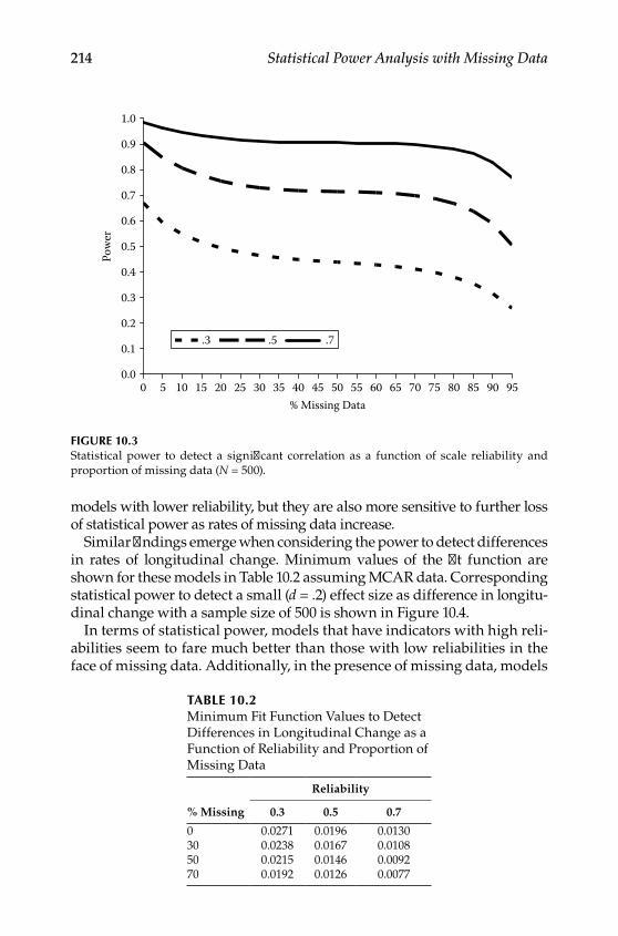
214 Statistical Power Analysis with Missing Data
models with lower reliability, but they are also more sensitive to further loss of statistical power as rates of missing data increase.
Similar findings emerge when considering the power to detect differences in rates of longitudinal change. Minimum values of the fit function are shown for these models in Table 10.2 assuming MCAR data. Corresponding statistical power to detect a small (d = .2) effect size as difference in longitu‑dinal change with a sample size of 500 is shown in Figure 10.4.
In terms of statistical power, models that have indicators with high reli‑abilities seem to fare much better than those with low reliabilities in the face of missing data. Additionally, in the presence of missing data, models
Table 10.2Minimum Fit Function Values to Detect Differences in Longitudinal Change as a Function of Reliability and Proportion of Missing Data
Reliability
% Missing 0.3 0.5 0.7
0 0.0271 0.0196 0.013030 0.0238 0.0167 0.010850 0.0215 0.0146 0.009270 0.0192 0.0126 0.0077
0.0
0.1
0.2
0.3
0.4
0.5
0.6
0.7
0.8
0.9
1.0
% Missing Data0 5 10 15 20 25 30 35 40 45 50 55 60 65 70 75 80 85 90 95
Pow
er
.3 .5 .7
Figure 10.3Statistical power to detect a significant correlation as a function of scale reliability and proportion of missing data (N = 500).
Y100315.indb 214 7/15/09 3:00:17 PM
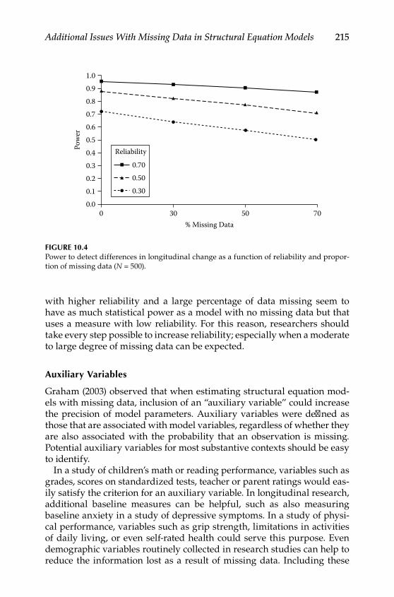
Additional Issues With Missing Data in Structural Equation Models 215
with higher reliability and a large percentage of data missing seem to have as much statistical power as a model with no missing data but that uses a measure with low reliability. For this reason, researchers should take every step possible to increase reliability; especially when a moderate to large degree of missing data can be expected.
auxiliary Variables
Graham (2003) observed that when estimating structural equation mod‑els with missing data, inclusion of an “auxiliary variable” could increase the precision of model parameters. Auxiliary variables were defined as those that are associated with model variables, regardless of whether they are also associated with the probability that an observation is missing. Potential auxiliary variables for most substantive contexts should be easy to identify.
In a study of children’s math or reading performance, variables such as grades, scores on standardized tests, teacher or parent ratings would eas‑ily satisfy the criterion for an auxiliary variable. In longitudinal research, additional baseline measures can be helpful, such as also measuring baseline anxiety in a study of depressive symptoms. In a study of physi‑cal performance, variables such as grip strength, limitations in activities of daily living, or even self‑rated health could serve this purpose. Even demographic variables routinely collected in research studies can help to reduce the information lost as a result of missing data. Including these
1.00.90.80.70.60.5
Reliability
0.700.500.30
Pow
er
0.40.30.20.10.0
0 30% Missing Data
50 70
Figure 10.4Power to detect differences in longitudinal change as a function of reliability and propor‑tion of missing data (N = 500).
Y100315.indb 215 7/15/09 3:00:17 PM

216 Statistical Power Analysis with Missing Data
auxiliary variables in models reduces the confidence intervals associated with model parameters.
To illustrate the effects of including an auxiliary variable on the rate of decrease in statistical power associated with missing data, we generated a variable that was associated with initial scores but unrelated to the missing data mechanism. This variable is added to the two‑group growth curve model described above. In order to examine the effects of the strength of association in moderating loss of statistical power, the auxiliary variable represented correlations ranging from .1 to .7 in increments of .2 for this study.
In Table 10.3 we show the minimum values of the fit function obtained for MCAR and MAR data under each condition. As can be seen, the results for MCAR and MAR data parallel each other fairly closely, typically dif‑fering only at the third or fourth decimal place.
Another more informative way to present these data is to plot their values as a function of their corresponding values in a model where the auxiliary variable is not included. We do this in Figure 10.5, plotting
Point of Reflection
In your area of research, there are likely to be quite a few variables that could serve as auxiliary variables. Take a few minutes to consider some possibili‑ties for what might work well for the kind of research you do. If you were pressed to come up with a “gold standard” auxiliary variable for each of your key outcome variables, what would it be?
Troubleshooting Tip
Using full information maximum likelihood, inclusion of auxiliary vari‑ables can very quickly convert even the most elegant path diagram into something more closely resembling spaghetti. Graham (2003) has several helpful suggestions for adding auxiliary variables to your models.
Try Me!
Use the values in Table 10.3 to determine what strength of auxiliary variable would be required to achieve power of .8 with 25% missing data with the sample sizes typical for your area of research.
Y100315.indb 216 7/15/09 3:00:17 PM
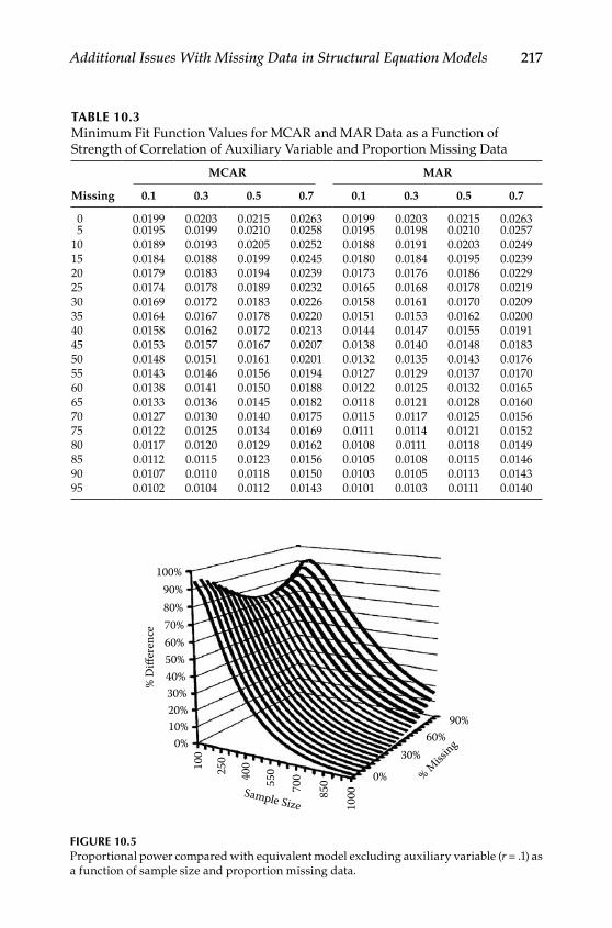
Additional Issues With Missing Data in Structural Equation Models 217
Table 10.3Minimum Fit Function Values for MCAR and MAR Data as a Function of Strength of Correlation of Auxiliary Variable and Proportion Missing Data
MCAR MAR
Missing 0.1 0.3 0.5 0.7 0.1 0.3 0.5 0.7
0 0.0199 0.0203 0.0215 0.0263 0.0199 0.0203 0.0215 0.0263 5 0.0195 0.0199 0.0210 0.0258 0.0195 0.0198 0.0210 0.025710 0.0189 0.0193 0.0205 0.0252 0.0188 0.0191 0.0203 0.024915 0.0184 0.0188 0.0199 0.0245 0.0180 0.0184 0.0195 0.023920 0.0179 0.0183 0.0194 0.0239 0.0173 0.0176 0.0186 0.022925 0.0174 0.0178 0.0189 0.0232 0.0165 0.0168 0.0178 0.021930 0.0169 0.0172 0.0183 0.0226 0.0158 0.0161 0.0170 0.020935 0.0164 0.0167 0.0178 0.0220 0.0151 0.0153 0.0162 0.020040 0.0158 0.0162 0.0172 0.0213 0.0144 0.0147 0.0155 0.019145 0.0153 0.0157 0.0167 0.0207 0.0138 0.0140 0.0148 0.018350 0.0148 0.0151 0.0161 0.0201 0.0132 0.0135 0.0143 0.017655 0.0143 0.0146 0.0156 0.0194 0.0127 0.0129 0.0137 0.017060 0.0138 0.0141 0.0150 0.0188 0.0122 0.0125 0.0132 0.016565 0.0133 0.0136 0.0145 0.0182 0.0118 0.0121 0.0128 0.016070 0.0127 0.0130 0.0140 0.0175 0.0115 0.0117 0.0125 0.015675 0.0122 0.0125 0.0134 0.0169 0.0111 0.0114 0.0121 0.015280 0.0117 0.0120 0.0129 0.0162 0.0108 0.0111 0.0118 0.014985 0.0112 0.0115 0.0123 0.0156 0.0105 0.0108 0.0115 0.014690 0.0107 0.0110 0.0118 0.0150 0.0103 0.0105 0.0113 0.014395 0.0102 0.0104 0.0112 0.0143 0.0101 0.0103 0.0111 0.0140
100%90%80%70%60%50%40%%
Diff
eren
ce
30%20%10%
Sample Size
% Miss
ing
0%
30%60%
90%
0%
100
250
400
550
700
850
1000
Figure 10.5Proportional power compared with equivalent model excluding auxiliary variable (r = .1) as a function of sample size and proportion missing data.
Y100315.indb 217 7/15/09 3:00:18 PM

218 Statistical Power Analysis with Missing Data
proportional power as a function of sample size and percent missing data. The associations are clearly nonlinear. Even with a very weak covariate (r = .1), there is considerable benefit to inclusion of an auxil‑iary variable.
Differences are largest at smaller sample sizes, and there is a further interaction such that differences are greatest with either higher or lower amounts of missing data for smaller sample sizes, but differences are greater at higher levels of missing data for larger sample sizes. In other words, including an auxiliary variable nearly doubles the statistical power at small sample sizes, with somewhat less pronounced increases with mod‑erate levels of missing data, whereas its effects at larger sample sizes tend to be more modest and limited to situations with higher levels of missing data. However, the former situation is one where it is most important to maximize statistical power, whereas the latter situation is one where ample statistical power is likely to exist, even with fairly extensive missing data.
There are many situations where it is easy to include useful auxiliary variables. For example, a researcher interested in depressive symptoms could include multiple measures of this construct or closely related con‑structs in a baseline wave and continue to reap benefits of this auxil‑iary variable in subsequent waves despite participant dropout. Likewise, inclusion of parent and teacher ratings in addition to self‑report measures obtained from children are likely to afford some protection against miss‑ing data, and these benefits are greater when the auxiliary variables cor‑relate more strongly with the variables of interest or on which missing data are expected. In general, Graham (2003) recommends inclusion of multiple auxiliary variables and presents straightforward ways to do so.
Conclusions
In this chapter, we extended consideration of statistical power with missing data to evaluation of model fit according to a wide variety of indices. Noncentrality‑based indices appear to show the greatest prom‑ise with missing data because they are not affected by missing data when a model is correctly specified. Under the typical circumstances where models are at least slightly misspecified, however, fit indices such as the RMSEA and TLI are biased toward indicating better model fit (i.e., less statistical power) as missing data increase, all else equal. Statistical power to reject incorrectly specified models also varies in part as a function of whether the models are acceptable (i.e., fairly minor or within the range of sampling variability) or unacceptable. We also illustrated how additional types of fit indices such as the RMR can
Y100315.indb 218 7/15/09 3:00:18 PM
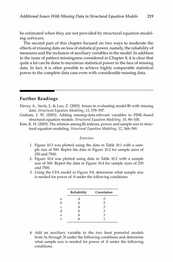
Additional Issues With Missing Data in Structural Equation Models 219
be estimated when they are not provided by structural equation model‑ing software.
The second part of this chapter focused on two ways to moderate the effects of missing data on loss of statistical power, namely, the reliability of measures and the inclusion of auxiliary variables in the model. In addition to the issue of pattern missingness considered in Chapter 8, it is clear that quite a lot can be done to maximize statistical power in the face of missing data. In fact, it is often possible to achieve highly comparable statistical power to the complete data case even with considerable missing data.
Further Readings
Davey, A., Savla, J., & Luo, Z. (2005). Issues in evaluating model fit with missing data. Structural Equation Modeling, 12, 578–597.
Graham, J. W. (2003). Adding missing‑data‑relevant variables to FIML‑based structural equation models. Structural Equation Modeling, 10, 80–100.
Kim, K. H. (2005). The relation among fit indexes, power, and sample size in struc‑tural equation modeling. Structural Equation Modeling, 12, 368–390.
Exercises
1. Figure 10.3 was plotted using the data in Table 10.1 with a sam‑ple size of 500. Replot the data in Figure 10.2 for sample sizes of 250 and 7500.
2. Figure 10.4 was plotted using data in Table 10.2 with a sample size of 500. Replot the data in Figure 10.4 for sample sizes of 250 and 7500.
3. Using the CFA model in Figure 9.8, determine what sample size is needed for power of .8 under the following conditions.
4. Add an auxiliary variable to the two least powerful models from 3a through 3f under the following conditions and determine what sample size is needed for power of .8 under the following conditions.
Reliability Correlation
a .4 .5b .8 .5c .4 .3d .8 .3e .4 .1f .8 .1
Y100315.indb 219 7/15/09 3:00:18 PM

220 Statistical Power Analysis with Missing Data
Syntax to Calculate RMR and SRMR
* RMR;OPTIONS LINESIZE=132 PAGESIZE=200 NOCENTER;
data s; infile 'c: \satcov.txt' lrecl=1200 missover dlm=','; input#1 s11 s21 s31 s41 s51 s61 s71 s81 s91 s22 s32 s42 s52 s62 s72 s82 s92 s33 s43 s53 s63 s73 s83 s93 s44 s54 s64 s74 s84 s94 s55 s65 s75 s85 s95 s66 s76 s86 s96 s77 s87 s97 s88 s98 s99 smean1 smean2 smean3 smean4 smean5 smean6 smean7 smean8 smean9 m it ; run;proc sort; by it; run;
data sigma; infile 'c:\ matrices.txt' lrecl=1200 missover dlm=','; input#1 l1 l2 l3 l4 l5 l6 l7 l8 l9 e1 e2 e3 e4 e5 e6 e7 e8 e9 xbar1 xbar2 xbar3 xbar4 xbar5 xbar6 xbar7 xbar8 xbar9 cov1 cov2 cov3 m it ; run;
data sigma2; set sigma;
z11=l1+e1; z21=l4*l1; z31=l5*l1; z41=cov1; z51=l6*cov1;
Auxiliary Correlation
a .1b .5c .9
Y100315.indb 220 7/15/09 3:00:18 PM

Additional Issues With Missing Data in Structural Equation Models 221
z61=l7*cov1; z71=cov3; z81=l8*cov3; z91=l9*cov3;
z22=(l4*l1*l4)+e2; z32=l5*l1*l4; z42=cov1*l4; z52=l6*cov1*l4; z62=l7*cov1*l4; z72=cov3*l4; z82=l8*cov3*l4; z92=l9*cov3*l4;
z33=(l5*l1*l5)+e3; z43=cov1*l5; z53=l6*cov1*l5; z63=l7*cov1*l5; z73=cov3*l5; z83=l8*cov3*l5; z93=l9*cov3*l5;
z44=l2+e4; z54=l6*l2; z64=l7*l2; z74=cov2; z84=l8*cov2; z94=l9*cov2;
z55=(l6*l2*l6)+e5; z65=l7*l2*l6; z75=cov2*l6; z85=l8*cov2*l6; z95=l9*cov2*l6;
z66=(l7*l2*l7)+e6; z76=cov2*l7; z86=l8*cov2*l7; z96=l9*cov2*l7;
z77=l3+e7; z87=l8*l3; z97=l9*l3;
z88=(l8*l3*l8)+e8; z98=l9*l3*l8;
z99=(l9*l3*l9)+e9;
Y100315.indb 221 7/15/09 3:00:18 PM

222 Statistical Power Analysis with Missing Data
run;
proc sort; by it; run;
data all; merge s sigma2; by it; run;
data diff; set all; r11=s11-z11; r21=s21-z21; r31=s31-z31; r41=s41-z41; r51=s51-z51; r61=s61-z61; r71=s71-z71; r81=s81-z81; r91=s91-z91;
r22=s22-z22; r32=s32-z32; r42=s42-z42; r52=s52-z52; r62=s62-z62; r72=s72-z72; r82=s82-z82; r92=s92-z92;
r33=s33-z33; r43=s43-z43; r53=s53-z53; r63=s63-z63; r73=s73-z73; r83=s83-z83; r93=s93-z93;
r44=s44-z44; r54=s54-z54; r64=s64-z64; r74=s74-z74; r84=s84-z84; r94=s94-z94;
r55=s55-z55; r65=s65-z65; r75=s75-z75;
Y100315.indb 222 7/15/09 3:00:18 PM

Additional Issues With Missing Data in Structural Equation Models 223
r85=s85-z85; r95=s95-z95;
r66=s66-z66; r76=s76-z76; r86=s86-z86; r96=s96-z96;
r77=s77-z77; r87=s87-z87; r97=s97-z97;
r88=s88-z88; r98=s98-z98; r99=s99-z99; rmr = sqrt((r11*r11+r21*r21+r31*r31+r41*r41+r51*r51+r61*r61+r71*r71+r81*r81+r91*r91+
r22*r22+r32*r32+r42*r42+r52*r52+r62*r62+r72*r72+r82*r82+r92*r92+
r33*r33+r43*r43+r53*r53+r63*r63+r73*r73+r83*r83+r93*r93+
r44*r44+r54*r54+r64*r64+r74*r74+r84*r84+r94*r94+
r55*r55+r65*r65+r75*r75+r85*r85+r95*r95+
r66*r66+r76*r76+r86*r86+r96*r96+
r77*r77+r87*r87+r97*r97+
r88*r88+r98*r98+
r99*r99)/45);run;
proc print; var rmr; run;
* SRMR;OPTIONS LINESIZE=132 PAGESIZE=200 NOCENTER;
data s; infile 'c:\satcov.txt' lrecl=1200 missover dlm=','; input#1 s11 s21 s31 s41 s51 s61 s71 s81 s91 s22 s32 s42 s52 s62 s72 s82 s92 s33 s43 s53 s63 s73 s83 s93
Y100315.indb 223 7/15/09 3:00:18 PM

224 Statistical Power Analysis with Missing Data
s44 s54 s64 s74 s84 s94 s55 s65 s75 s85 s95 s66 s76 s86 s96 s77 s87 s97 s88 s98 s99 smean1 smean2 smean3 smean4 smean5 smean6 smean7 smean8 smean9 m it ; run;
data s2; set s; sd11=sqrt(s11); sd22=sqrt(s22); sd33=sqrt(s33); sd44=sqrt(s44); sd55=sqrt(s55); sd66=sqrt(s66); sd77=sqrt(s77); sd88=sqrt(s88); sd99=sqrt(s99); sd21=s21/sd11/sd22; sd31=s31/sd11/sd33; sd41=s41/sd11/sd44; sd51=s51/sd11/sd55; sd61=s61/sd11/sd66; sd71=s71/sd11/sd77; sd81=s81/sd11/sd88; sd91=s91/sd11/sd99; sd32=s32/sd22/sd33; sd42=s42/sd22/sd44; sd52=s52/sd22/sd55; sd62=s62/sd22/sd66; sd72=s72/sd22/sd77; sd82=s82/sd22/sd88; sd92=s92/sd22/sd99; sd43=s43/sd33/sd44; sd53=s53/sd33/sd55; sd63=s63/sd33/sd66; sd73=s73/sd33/sd77; sd83=s83/sd33/sd88; sd93=s93/sd33/sd99; sd54=s54/sd44/sd55; sd64=s64/sd44/sd66; sd74=s74/sd44/sd77;
Y100315.indb 224 7/15/09 3:00:18 PM

Additional Issues With Missing Data in Structural Equation Models 225
sd84=s84/sd44/sd88; sd94=s94/sd44/sd99; sd65=s65/sd55/sd66; sd75=s75/sd55/sd77; sd85=s85/sd55/sd88; sd95=s95/sd55/sd99; sd76=s76/sd66/sd77; sd86=s86/sd66/sd88; sd96=s96/sd66/sd99; sd87=s87/sd77/sd88; sd97=s97/sd77/sd99; sd98=s98/sd88/sd99; run;
proc sort; by it; run;
data sigma; infile 'c:\matrices.txt' lrecl=1200 missover dlm=','; input#1 l1 l2 l3 l4 l5 l6 l7 l8 l9 e1 e2 e3 e4 e5 e6 e7 e8 e9 xbar1 xbar2 xbar3 xbar4 xbar5 xbar6 xbar7 xbar8 xbar9 cov1 cov2 cov3 m it ; run;
data sigma2; set sigma; z11=l1+e1; z21=l4*l1; z31=l5*l1; z41=cov1; z51=l6*cov1; z61=l7*cov1; z71=cov3; z81=l8*cov3; z91=l9*cov3;
z22=(l4*l1*l4)+e2; z32=l5*l1*l4; z42=cov1*l4; z52=l6*cov1*l4; z62=l7*cov1*l4; z72=cov3*l4; z82=l8*cov3*l4; z92=l9*cov3*l4;
z33=(l5*l1*l5)+e3;
Y100315.indb 225 7/15/09 3:00:18 PM

226 Statistical Power Analysis with Missing Data
z43=cov1*l5; z53=l6*cov1*l5; z63=l7*cov1*l5; z73=cov3*l5; z83=l8*cov3*l5; z93=l9*cov3*l5;
z44=l2+e4; z54=l6*l2; z64=l7*l2; z74=cov2; z84=l8*cov2; z94=l9*cov2;
z55=(l6*l2*l6)+e5; z65=l7*l2*l6; z75=cov2*l6; z85=l8*cov2*l6; z95=l9*cov2*l6;
z66=(l7*l2*l7)+e6; z76=cov2*l7; z86=l8*cov2*l7; z96=l9*cov2*l7;
z77=l3+e7; z87=l8*l3; z97=l9*l3;
z88=(l8*l3*l8)+e8; z98=l9*l3*l8;
z99=(l9*l3*l9)+e9;
run;
data sigma3; set sigma2; zd11=sqrt(z11); zd22=sqrt(z22); zd33=sqrt(z33); zd44=sqrt(z44); zd55=sqrt(z55); zd66=sqrt(z66); zd77=sqrt(z77); zd88=sqrt(z88); zd99=sqrt(z99); zd21=z21/zd11/zd22;
Y100315.indb 226 7/15/09 3:00:18 PM

Additional Issues With Missing Data in Structural Equation Models 227
zd31=z31/zd11/zd33; zd41=z41/zd11/zd44; zd51=z51/zd11/zd55; zd61=z61/zd11/zd66; zd71=z71/zd11/zd77; zd81=z81/zd11/zd88; zd91=z91/zd11/zd99; zd32=z32/zd22/zd33; zd42=z42/zd22/zd44; zd52=z52/zd22/zd55; zd62=z62/zd22/zd66; zd72=z72/zd22/zd77; zd82=z82/zd22/zd88; zd92=z92/zd22/zd99; zd43=z43/zd33/zd44; zd53=z53/zd33/zd55; zd63=z63/zd33/zd66; zd73=z73/zd33/zd77; zd83=z83/zd33/zd88; zd93=z93/zd33/zd99; zd54=z54/zd44/zd55; zd64=z64/zd44/zd66; zd74=z74/zd44/zd77; zd84=z84/zd44/zd88; zd94=z94/zd44/zd99; zd65=z65/zd55/zd66; zd75=z75/zd55/zd77; zd85=z85/zd55/zd88; zd95=z95/zd55/zd99; zd76=z76/zd66/zd77; zd86=z86/zd66/zd88; zd96=z96/zd66/zd99; zd87=z87/zd77/zd88; zd97=z97/zd77/zd99; zd98=z98/zd88/zd99;run;
proc sort; by it; run;
data all; merge s2 sigma3; by it;run;
data diff; set all; rd11=sd11-zd11; rd21=sd21-zd21;
Y100315.indb 227 7/15/09 3:00:18 PM

228 Statistical Power Analysis with Missing Data
rd31=sd31-zd31; rd41=sd41-zd41; rd51=sd51-zd51; rd71=sd71-zd71; rd81=sd81-zd81; rd91=sd91-zd91;
rd22=sd22-zd22; rd32=sd32-zd32; rd42=sd42-zd42; rd52=sd52-zd52; rd62=sd62-zd62; rd72=sd72-zd72; rd82=sd82-zd82; rd92=sd92-zd92;
rd33=sd33-zd33; rd43=sd43-zd43; rd53=sd53-zd53; rd63=sd63-zd63; rd73=sd73-zd73; rd83=sd83-zd83; rd93=sd93-zd93;
rd44=sd44-zd44; rd54=sd54-zd54; rd64=sd64-zd64; rd74=sd74-zd74; rd84=sd84-zd84; rd94=sd94-zd94;
rd55=sd55-zd55; rd65=sd65-zd65; rd75=sd75-zd75; rd85=sd85-zd85; rd95=sd95-zd95;
rd66=sd66-zd66; rd76=sd76-zd76; rd86=sd86-zd86; rd96=sd96-zd96;
rd77=sd77-zd77; rd87=sd87-zd87; rd97=sd97-zd97;
rd88=sd88-zd88; rd98=sd98-zd98;
Y100315.indb 228 7/15/09 3:00:18 PM

Additional Issues With Missing Data in Structural Equation Models 229
rd99=sd99-zd99;
srmr = sqrt((rd11*rd11+rd21*rd21+rd31*rd31+rd41*rd41+rd51*rd51+rd61*rd61+rd71*rd71+rd81*rd81+rd91*rd91+
rd22*rd22+rd32*rd32+rd42*rd42+rd52*rd52+rd62*rd62+rd72*rd72+rd82*rd82+rd92*rd92+
rd33*rd33+rd43*rd43+rd53*rd53+rd63*rd63+rd73*rd73+rd83*rd83+rd93*rd93+
rd44*rd44+rd54*rd54+rd64*rd64+rd74*rd74+rd84*rd84+rd94*rd94+
rd55*rd55+rd65*rd65+rd75*rd75+rd85*rd85+rd95*rd95+
rd66*rd66+rd76*rd76+rd86*rd86+rd96*rd96+ rd77*rd77+rd87*rd87+rd97*rd97+
rd88*rd88+rd98*rd98+
rd99*rd99)/45); run; proc print; var srmr; run;
Y100315.indb 229 7/15/09 3:00:18 PM

Y100315.indb 230 7/15/09 3:00:18 PM
231
11Summary and Conclusions
In this book, we have tried to provide a step by step guide to planning, implementing, and interpreting a power analysis when the researcher expects missing data, focusing on a structural equation modeling per‑spective. The broad set of tools that we have outlined can be applied to measurement models, structural models, or any combination thereof and work equally well whether data are missing completely at random (MCAR) or missing at random (MAR). Although beyond the scope of this volume because it also introduces issues related to bias in parameter esti‑mates, the methods we describe can also quite easily be extended to situ‑ations where data are missing not at random (MNAR) by generating a missing data mechanism that is not completely included in the analytic model itself.
Wrapping Up
In terms of fundamentals, taking stock of the wide set of skills and top‑ics we considered, the reader should now have the ability to identify factors associated with statistical power, be fluent with the fundamen‑tals of structural equation modeling, and have a broad understanding of different ways in which statistical power can be conceptualized and operationalized. In terms of applications, the reader should have a thor‑ough understanding of the role of selection in affecting means, variances, and covariances in different segments of a population and the ability to apply principles of power analysis to a wide variety of models, missing data mechanisms, and with methods that are either population based or empirical, such as in the design and implementation of a full‑scale Monte Carlo study, with either normally or nonnormally distributed data.
We have also begun the process of considering several important exten‑sions to these approaches. Particular attention was paid to the issue of evaluating model fit using indices beyond the global model chi‑square. Evaluating model fit is an important and complex topic in structural
Y100315.indb 231 7/15/09 3:00:18 PM

232 Statistical Power Analysis with Missing Data
equation modeling generally, and we saw that many of these issues are compounded when some of the data are unobserved. We also saw that issues such as which patterns of data are observed, scale reliability, and inclusion of an auxiliary variable can have critical implications for the effects of missing data on the loss of statistical power. In particular, careful exploitation of these issues can ensure that power remains as high as pos‑sible, even under circumstances that are less than ideal. All of the materi‑als and methods described in this book just begin to scratch the surface of the work that remains ahead and the potential to elaborate and improve upon these techniques. Several promising directions remain relatively unexplored.
Future Directions
We noted in Chapter 2 of this book that many aspects of structural equa‑tion modeling software have converged in recent years, such as the ability to handle missing data or to specify models in matrix, equation, or graphi‑cal form. Another important area of emphasis that we did not consider in great detail is that there are many important extensions of structural equation models that are also becoming more commonly applied but are not yet consistently available across software packages. These include, for example, the ability to include sampling and design weights in anal‑yses (both of which have implications for statistical power), the ability to analyze nested data structures (such as individuals within dyads or over time, or in larger social structures such as classrooms), the ability to include nominal, dichotomous, and ordinal manifest and latent variables, multiple latent and observed classes that are useful for mixture models, and even extensions of the estimation methods themselves.
There is growing interest, for example, in Bayesian methods for struc‑tural equation modeling, and AMOS has implemented Bayesian estima‑tion in its most recent version. Lee (e.g., 2007, Lee & Song, 2004; Lee & Tang, 2006) has written extensively on this topic. Because by nature it involves Monte Carlo methods and can be readily extended to very complex situ‑ations involving missing data, this is likely to be an increasingly impor‑tant tool for researchers interested in power analysis within the structural equation modeling framework.
Similarly, progress has been made in terms of identifying robust esti‑mators for structural equation models (Moustaki & Victoria‑Feser, 2006) that can provide very useful extensions with nonnormally distributed data. Likewise, there have been important extensions on the mathemati‑cal side of power calculations with missing data. Brown, Indurkhya, and
Y100315.indb 232 7/15/09 3:00:19 PM
Summary and Conclusions 233
Kellam (2000) “solved” the power equations for one set of models. Though the equations for the relatively simple set of models they consider span more than four manuscript pages, the approach itself is extremely useful for researchers who need to understand a specific design in considerable depth. In the case of their research, they were able to identify ways to pro‑tect their data against nonignorably missing data in a longitudinal study on the effects of lead exposure.
Conclusions
In conclusion, we hope that this volume has provided readers with the tools they need to begin incorporating missing data into their power calculations to a greater extent than previously. Though no volume can hope to be all things to all readers, we hope that every reader is able to find something of value in their own research. In particular, we hope that by beginning simply from first principles, but without skimp‑ing on the underlying mathematical elements, even readers without a strong background in statistics can very quickly increase their knowl‑edge to the point where they become more comfortable staying abreast of developments in these areas with the ability to apply them in their own work.
Further Readings
Brown, C. H., Indurkhya, A., & Kellam, S. G. (2000). Power calculations for data missing by design: Applications to a follow‑up study of lead exposure and attention. Journal of the American Statistical Association, 95, 383–395.
Lee, S.‑Y. (2007). Structural equation modeling: A Bayesian approach. New York: Wiley.Molenberghs, G., & Kenward, M. (2007). Missing data in clinical studies. New
York: Wiley.
Y100315.indb 233 7/15/09 3:00:19 PM

Y100315.indb 234 7/15/09 3:00:19 PM

235
References
Abadir, K.M., & Magnus, J. R. (2005). Matrix algebra. New York: Cambridge.Abraham, W. T., & Russell, D. W. (2008). Statistical power analysis in psychological
research. Social and Personality Psychology Compass, 2, 283–301.Acock, A. C. (2005). Working with missing values. Journal of Marriage and Family,
67, 1012–1028.Allison, P. D. (1987). Estimation of linear models with incomplete data. In C. C.
Clog (Ed.), Sociological methodology (pp. 71–103). San Francisco: Jossey‑Bass.Allison, P. D. (2001). Missing data. Thousand Oaks, CA: Sage.Anderson, E. R. (1993). Analyzing change in short‑term longitudinal research
using cohort‑sequential designs. Journal of Consulting and Clinical Psychology, 61, 929–940.
Anderson, T. W. (1957). Maximum likelihood estimates for a multivariate normal distribution when some observations are missing. Journal of the American Statistical Association, 52, 200–203.
Arbuckle, J. L. (1996). Full information estimation in the presence of incomplete data. In G. A. Maculates & R. E. Schumacker (Eds.), Advanced structural equa‑tion modeling: Issues and techniques (pp. 243–277). Mahwah, NJ: Erlbaum.
Arbuckle, J. L. (2006). AMOS user’s guide 7.0. Chicago, IL: SPSS.Bandalos, D. L. (2006). The use of Monte Carlo studies in structural equation mod‑
eling. In G. R. Hancock & R. O. Mueller (Eds), Structural equation modeling: A second course (pp. 385–426). Greenwich, CT: Information Age.
Bell, R. Q. (1953). Convergence: An accelerated longitudinal approach. Child Development, 24, 145–152.
Bell, R. Q. (1954). An experimental test of the accelerated longitudinal approach. Child Development, 25, 281–286.
Bentler, P. M. (1990). Comparative fit indexes in structural models. Psychological Bulletin, 107, 238–246.
Bentler, P. M. (1995). EQS structural equations program manual. Encino, CA: Multivariate Software, Inc.
Bentler, P. M., & Bonett, D. G. (1980). Significance tests and goodness of fit in the analysis of covariance structures. Psychological Bulletin, 88, 588–606.
Bollen, K. A. (1989a). A new incremental fit index for general structural equation models. Sociological Methods and Research, 17, 303–316.
Bollen, K. A. (1989b). Structural equations with latent variables. New York: Wiley.Boomsma, A. (2000). Reporting analyses of covariance structures. Structural
Equation Modeling, 7, 461–483.Brown, C. H., Indurkhya, A., & Kellam, S. G. (2000). Power calculations for data
missing by design: Applications to a follow‑up study of lead exposure and attention. Journal of the American Statistical Association, 95, 383–395.
Y100315.indb 235 7/15/09 3:00:19 PM

236 References
Brown, M. W., & Cudeck, R. (1993). Alternative ways of assessing model fit. In K. A. Bollen & J. S. Long (Eds.) Testing structural equation models (pp. 136–162). Thousand Oaks, CA: Sage.
Burr, I. W. (1942). Cumulative frequency functions. Annals of Mathematical Statistics, 13, 215–232.
Byrne, B. M. (1998). Structural equation modeling with LISREL, PRELIS, and SIMPLIS: Basic concepts, applications, and programming. Mahwah, NJ: Erlbaum.
Campbell, D. T., & Stanley, J. C. (1963). Experiments and quasi‑experimental designs for research. Skokie, IL: Rand McNally.
Cleary, T. A., & Linn, R. L. (1969). Error of measurement and the power of a sta‑tistical test. The British Journal of Mathematical and Statistical Psychology, 22, 49–55.
Cohen, J. H. (1969). Statistical power analysis for the behavioral sciences. New York: Academic Press.
Cohen, J. H. (1988). Statistical power analysis for the behavioral sciences (2nd ed.). Hillsdale, NJ: Erlbaum.
Cohen, J. H. (1992). A power primer. Psychological Bulletin, 112, 115–159.Cole, D. A., Maxwell, S. E., Arvey, R., & Salas, E. (1993). Multivariate group com‑
parisons of variable systems: MANOVA and structural equation modeling. Psychological Bulletin, 114, 174–184.
Collins, L. M., Murphy, S. A., & Bierman, K. (2004). A conceptual framework for adaptive preventive interventions. Prevention Science, 5, 185–196.
Curran, P. J., & Muthén, B. O. (1999). The application of latent curve analysis to testing developmental theories in intervention research. American Journal of Community Psychology, 27(4), 1999.
Davey, A. (2001). An analysis of incomplete data. In L. M. Collins & A. G. Sayer (Eds.), New methods for the analysis of change (pp. 379–383). Washington, DC: American Psychological Association.
Davey, A., & Savla, J. (2009). Evaluating statistical power with incomplete data. Organizational Research Methods, 12, 320–346.
Davey, A., Savla, J. S., & Luo, Z. (2005). Issues in evaluating model fit with missing data. Structural Equation Modeling, 12, 578–597.
Dempster, A. P., Laird, N. M., & Rubin, D. B. (1977). Maximum likelihood from incomplete data via the EM algorithm. Journal of the Royal Statistical Society, Series B, 39, 1–38.
Dolan, C., van der Sluis, S., & Grasman, R. (2005). A note on normal theory power calculation in structural equation modeling with data missing completely at random. Structural Equation Modeling, 12, 245–262.
Dolan, C. V., & Molenaar, P. C. M. (1994). Testing specific hypotheses concerning latent group differences in multi‑group covariance structure analysis with structured means. Multivariate Behavioral Research, 29, 203–222.
Dolan, C. V., Molenaar, P. C. M., & Boomsma, D. I. (1994). Simultaneous genetic analysis of means and covariance structure: Pearson‑Lawley selection rules. Behavior Genetics, 24, 17–24.
Duncan, S. C., Duncan, T. E., & Strycker, L. A. (2002). A multilevel analysis of neighborhood context and youth alcohol and drug problems. Prevention Science, 3, 125–134.
Y100315.indb 236 7/15/09 3:00:19 PM
References 237
Duncan, T. E., Duncan, S. C., & Hops, H. (1996). Analysis of longitudinal data within accelerated longitudinal designs. Psychological Methods, 1, 236–248.
Duncan, T. E., Duncan, S. C., Strycker, L. A., Li, F., & Alpert. A. (2006). An introduc‑tion to latent variable growth curve modeling: Concepts, issues, and applications (2nd ed.). Mahwah, NJ: Lawrence Erlbaum.
Efron, B., & Tibshirani, R. (1993). An introduction to the bootstrap. Boca Raton, FL: CRC Press.
Egger, M., Davey Smith, G., & Altman, D. (2001). Systematic reviews in health care: Meta‑analysis in context. London: BMJ Publishing.
Enders, C. K., & Bandalos, D. L. (2001). The relative performance of full informa‑tion maximum likelihood estimation for missing data in structural equation models. Structural Equation Modeling, 8, 430–457.
Fan, X. (2003). Power of latent growth modeling for detecting group differences in linear growth trajectory parameters. In Structural equation modeling (Vol. 10, pp. 380–400). Mahwah, NJ: Lawrence Erlbaum.
Fan, X., Felsővályi, Á., Sivo, S. A., & Keenan, S. C. (2001). SAS for Monte Carlo stud‑ies: A guide for quantitative researchers. Cary, NC: SAS Institute.
Faul, F., Erdfelder, E., Lang, A.‑G., & Buchner, A. (2007). G*Power 3: A flexible statistical power analysis program for the social, behavioral, and biomedical sciences. Behavior Research Methods, 39, 175–191.
Fleishman, A. I. (1978). A method for simulating non‑normal distributions. Psychometrika, 43, 521–532.
Fleiss, J. L. (1976). Comment on Overall and Woodard’s asserted paradox concern‑ing the measurement of change. Psychological Bulletin, 83, 774–775.
Fox, J. (2006). Structural equation modeling with the SEM package in R. Structural Equation Modeling, 13, 465–486.
Fox, J. (2009). A mathematical primer for social statistics. Thousand Oaks, CA: Sage.Gerbing, D. W., & Anderson, J. C. (1993). Monte Carlo evaluations of goodness‑of‑fit
indices for structural equation models. In K. A. Bollen (Ed.), Testing structual equation models (pp. 40–65). Newbury Park, CA: Sage.
Gonzalez, R., & Griffin, D. (2001). Testing parameters in structural equation mod‑eling: Every “one” matters. Psychological Methods, 6, 258–269.
Graham, J. W. (2003). Adding missing‑data‑relevant variables to FIML‑based structural equation models. Structural Equation Modeling, 10, 80–100.
Graham, J. W. (2009). Missing data analysis: Making it work in the real world. Annual Review of Psychology, 60, 549–576.
Graham, J. W., Hofer, S. M., & MacKinnon, D. P. (1996). Maximizing the useful‑ness of data obtained with planned missing value patterns: An application of maximum likelihood procedures. Multivariate Behavioral Research, 31, 197–218.
Graham, J. W., Olchowski, A. E., & Gilreath, T. D. (2007). How many imputations are really needed? Some practical clarifications of multiple imputation the‑ory. Prevention Science, 8, 206–213.
Graham, J. W., Taylor, B. J., & Cumsille, P. E. (2001). Planned missing data designs in analysis of change. In L. Collins & A. Sayer (Eds.), New meth‑ods for the analysis of change (pp. 335–353). Washington, DC: American Psychological Association.
Y100315.indb 237 7/15/09 3:00:19 PM
238 References
Graham, J. W., Taylor, B. J., Olchowski, A. E., & Cumsille, P. E. (2006). Planned missing data designs in psychological research. Psychological Methods, 11, 323–343.
Greene, W. H. (2007). Econometric analysis (4th ed.). Upper Saddle River, NJ: Prentice‑Hall.
Grissom, R. J., & Kim, J. J. (2005). Effect sizes for research: A broad practical approach. Mahwah, NJ: Erlbaum.
Hancock, G. R. (2006). Power analysis in covariance structure modeling. In G. R. Hancock & R. O. Mueller (Eds.), A second course in structural equation modeling (pp. 313–344). Greenwich, CT: Information Age.
Harlow, L. L., Mulaik, S. A., & Steiger, J. H. (1997). What if there were no significance tests? Mahwah, NJ: Elrbaum.
Hayduk, L. A. (1987). Structural equation modeling with LISREL: Essentials and advances. Baltimore, MD: Johns Hopkins.
Headrick, T. C., & Mugdadi, A. (2006). On simulating multivariate non‑normal dis‑tributions from the generalized lambda distribution. Computational Statistics and Data Analysis, 50, 3343–3353.
Heckman, J. J. (1979). Sample selection bias as a specification error. Econometrica, 47, 153–162.
Hedeker, D., & Gibbons, R. D. (1997). Application of random‑effects pattern‑mix‑ture models for missing data in longitudinal studies. Psychological Methods, 2, 64–78.
Hoyle, R. H. (1995). Structural equation modeling: Concepts, issues, and applications. Thousand Oaks, CA: Sage.
Hu, L., & Bentler, P. M. (1995). Evaluating model fit. In R. H. Hoyle (Ed.), Structural equation modeling: Issues, concepts, and applications (pp. 76–99). Newbury Park, CA: Sage.
Humphreys, L. G., & Drasgow, F. (1989). Some comments on the relation between reliability and statistical power. Applied Psychological Measurement, 13, 419–425.
Jamshidian, M., & Bentler, P. M. (1999). ML estimation of mean and covari‑ance structures with missing data using complete data routines. Journal of Educational and Behavioral Statistics, 24, 21–41.
Jöreskog, K. (1969). A general approach to confirmatory maximum likelihood fac‑tor analysis. Psychometrika, 34, 183–202.
Jöreskog, K. (1970). A general method for analysis of covariance structures. Biometrika, 57, 239–251.
Jöreskog, K. (1978). Structural analysis of covariance and correlation matrices. Psychometrika, 43, 443–477.
Jöreskog, K., & Sörbom, D. (2000). LISREL [Computer software]. Lincolnwood, IL: Scientific Software, Inc.
Jöreskog, K. G., & Sörbom, D. (1996). LISREL 8: User’s reference guide. Chicago: Scientific Software.
Juster, F. T., & Suzman, R. (1995). An overview of health and retirement study. Journal of Human Resources, 30, S7–S56.
Kaplan, D. (1995). Statistical power in structural equation modeling. In R. H. Hoyle (Ed.), Structural equation modeling: Concepts, issues, and applications (pp. 100–117). Newbury Park, CA: Sage.
Y100315.indb 238 7/15/09 3:00:19 PM
References 239
Kaplan, D. (2009). Structural equation modeling: Foundations and extensions. Thousand Oaks, CA: Sage.
Kelloway, E. K. (1998). Using LISREL for structural equation modeling: A researcher’s guide. Thousand Oaks, CA: Sage.
Kim, K. H. (2005). The relation among fit indexes, power, and sample size in struc‑tural equation modeling. Structural Equation Modeling, 12, 368–390.
LaDu, T. J., & Tanaka, J. S. (1995). Incremental fit index changes for nested struc‑tural equation models. Multivariate Behavioral Research, 30, 289–316.
Lee, S.‑K. (2007). Structural equation modeling: A Bayesian approach. New York: Wiley.Lee, S.‑K., & Song, X. Y. (2004). Bayesian model comparison of nonlinear structural
equation models with missing continuous and ordinal data. British Journal of Mathematical and Statistical Psychology, 57, 131–150.
Lee, S.‑K., & Tang, N.‑S. (2006). Bayesian analysis of nonlinear structural equation models with nonignorable missing data. Psychometrika, 71, 541–564.
Lipsey, M. W. (1990). Design sensitivity: Statistical power for experimental research. Newbury Park, CA: Sage.
Lipsey, M. W., & Wilson, D. B. (1993). The efficacy of psychological, educational, behavioral treatment: Confirmation from meta analysis. American Psychologist, 48, 1181–1209.
Lipsey, M. W., & Wilson, D. B. (2001). Practical meta‑analysis. Thousand Oaks, CA: Sage.
Little, R. J. A., & Rubin, D. B. (1989). The analysis of social science data with miss‑ing values. Sociological Methods and Research, 18, 292–326.
Little, R. J. A., & Rubin, D. B. (2002). Analysis with missing data (2nd ed.). New York: Wiley.
Little, T. D. (1997). Mean and covariance structures (MACS) analyses of cross‑cultural data: Practical and theoretical issues. Multivariate Behavioral Research, 32, 53–76.
Long, J. S. (2008). The workflow of data analysis using Stata. College Station, TX: Stata Press.
Luo, Z., Davey, A., & Savla, J. S. (2005, May). Missing data reduces statistical power in structural equation models using FIML. Paper presented at the American Psychological Society, Los Angeles, CA.
MacCallum, R. C., Browne, M. W., & Cai, L. (2006). Testing differences between nested covariance structure models: Power analysis and null hypotheses. Psychological Methods, 11, 19–35.
MacCallum, R. C., Browne, M. W., & Sugawara, H. M. (1996). Power analysis and determination of sample size for covariance structure modeling. Psychological Methods, 1(2), 130–149.
Marsh, H. W., Balla, J. R., & Hau, K. (1996). An evaluation of incremental fit indices: A clarification of mathematical and empirical properties. In G. A. Marcoulides & R. E. Schumacker (Eds.), Advanced structural equation model‑ing: Issues and techniques (pp. 315–351). Mahwah, NJ: Lawrence Erlbaum.
Marsh, H. W., Hau, K.‑T., & Wen, Z. (2004). In search of golden rules: Comment on hypothesis‑testing approaches to setting cutoff values for fit indexes and dangers in overgeneralizing Hu and Bentler’s (1999) findings. Structural Equation Modeling, 11, 320–341.
Mattson, S. (1997). How to generate non‑normal data for simulation of structural equation models. Multivariate Behavioral Research, 32, 355–373.
Y100315.indb 239 7/15/09 3:00:19 PM

240 References
Maxwell, S. E. (2004). The persistence of underpowered studies in psychological research: Causes, consequences, and remedies. Psychological Methods, 9, 147–163.
Maxwell, S. E., Cole, D. A., Arvey, R. D., & Salas, E. (1991). A comparison of methods for increasing power in randomized between‑subjects designs. Psychological Bulletin, 110(2), 328–337.
Maxwell, S. E., Kelly, K., & Rausch, J. R. (2008). Sample size planning for statistical power and accuracy in estimation. Annual Review of Psychology, 59, 537–563.
McArdle, J. J. (1994). Structural factor analysis experiments with incomplete data. In Multivariate Behavioral Research, 29, 409–454.
McArdle, J. J., & Hamagami, F. (1991). Modeling incomplete longitudinal and cross‑section data using latent growth structural models. In L. M. Collins & J. L. Horn (Eds.), Best methods for the analysis of change: Recent advances, unan‑swered questions, future directions (pp. 276–298). Washington, DC: American Psychological Association.
McArdle, J. J., & McDonald, R. P. (1984). Some algebraic properties of the reticu‑lar action model for moment structures. British Journal of Mathematical and Statistical Psychology, 37, 234–251.
McDonald, R. P. (1989). An index of goodness‑of‑fit based on noncentrality. Journal of Classification, 6, 97–103.
McDonald, R. P., & Marsh, H. W. (1990). Choosing a multivariate model: Noncentrality and goodness of fit. Psychological Bulletin, 107, 247–255.
Mehta, P. D., West, S. G. (2000). Putting the individual back in individual growth curves. Psychological Methods, 5, 23–43.
Meng, X.‑L., & Rubin, D. B. (1991). Using EM to obtain asymptotic variance‑co‑variance matrices: The SEM algorithm. Journal of the American Statistical Association, 86, 899–909.
Meng, X.‑L., & Rubin, D. B. (1992). Performing likelihood ratio tests with multi‑ply‑imputed data sets. Biometrika, 79, 103–111.
Metropolis, N. (1987). The beginning of the Monte Carlo method, Los Alamos Science, 15, 125–130.
Millsap, R. E., & Kwok, O.‑M. (2004). Evaluating the impact of partial factorial invariance on selection in two populations. Psychological Methods, 9, 93–115.
Molenberghs, G., & Kenward, M. G. (2007). Missing data in clinical studies. Hoboken, NJ: Wiley.
Moustaki, I., & Victoria‑Feser, M.‑P. (2006). Bounded‑influence robust estimation in generalized linear latent variable models. Journal of the American Statistical Association, 101, 644–653.
Mulaik, S. A., James, L. R., Van Alstine, J., Bennett, N., Lind, S., & Stilwell, C. D. (1989). Evaluation of goodness‑of‑fit indices for structural equation models. Psychological Bulletin, 105, 430–445.
Murphy, K. R., & Myors, B. (2004). Statistical power analysis: A simple and general model for traditional and modern hypothesis tests. Mahwah, NJ: L. Erlbaum.
Muthén, B., & Kaplan, D. (1985). A comparison of some methodologies for the fac‑tor analysis of non‑normal Likert variables. British Journal of Mathematical and Statistical Psychology, 38, 171–189.
Muthén, B. O., & Curran, P. J. (1997). General growth modeling of individual dif‑ferences in experimental designs: A latent variable framework for analysis and power estimation. Psychological Methods, 2, 371–402.
Y100315.indb 240 7/15/09 3:00:19 PM

References 241
Muthén, B. O., Kaplan, D., & Hollis, M. (1987). On structural equation modeling with data that are not missing completely at random. Psychometrika, 52, 431–462.
Muthén, L. K., & Muthén, B. O. (2002). How to use a Monte Carlo study to decide on sample size and determine power. Retrieved December 10, 2007, from http://www.statmodel.com/download/FinalSEMsingle.pdf
Muthén, L. K., & Muthén, B. O. (2007). MPlus statistical analysis with latent variables user’s guide. Los Angeles: Author.
Namboodiri, K. (1984). Matrix algebra: An introduction. Thousand Oaks, CA: Sage.Neale, M. C., Boker, S. M., Xie, G., & Maes, H. H. (2004). Mx: Statistical modeling.
Richmond: Virginia Commonwealth University.Neyman, J., & Pearson, E. S. (1928a). On the use of and interpretation of certain test
criteria for purposes of statistical inference. Part I. Biometrika, 20A, 175–240. Neyman, J., & Pearson, E. S. (1928b). On the use and interpretation of certain test
criteria for purposes of statistical inference. Part II. Biometrika, 20A, 263–294.Nicewander, W. A., & Price, J. M. (1978). Dependent variable reliability and the
power of significance tests. Psychological Bulletin, 85, 405–409.Overall, J. E. (1989). Distinguishing between measurements and dependent vari‑
ables. Applied Psychological Measurement, 13, 432–433.Overall, J. E., & Woodard, J. A. (1975). Unreliability of difference scores: A paradox
of measurement of change. Psychological Bulletin, 82, 85–86.Paxton, P., Curran, P. J., Bollen, K. A., Kirby, J., & Chen, F. (2001) Monte Carlo
experiments: Design and implementation. Structural Equation Modeling, 8, 287–312.
Pearson, K. (1903). Mathematical contributions to the theory of evolution XI: On the influence of natural selection on the variability and correlation of organs. Philosophical Transactions of the Royal Society of London: Series A, 200, 1–66.
Pearson, K. (1912). On the general theory of the influence of selection on correla‑tion and variation. Biometrika, 8, 437–443.
Rabe‑Hesketh, S., Skrondal, A., & Pickles, A. (2004). Generalized multilevel struc‑tural equation modelling. Psychometrika, 69, 183–206.
Ramberg, J., & Schmeiser, B. (1974). An approximate method for generating asym‑metric random variables. Communications of the ACM, 17, 78–82.
Raudenbush, S. W., & Chan, W. S. (1992). Growth curve analysis in accelerated lon‑gitudinal designs. Journal of Research in Crime and Delinquency, 29, 387–411.
Raudenbush, S. W., & Bryk, A. S. (2002). Hierarchical linear models: Applications and data analysis methods (2nd ed.). Newbury Park, CA: Sage.
Raykov, T., & Marcoulides, G. A. (2006). A first course in structural equation modeling. Mahwah, NJ: Erlbaum.
Saris, W. E., & Satorra, A. (1993). Power evaluations in structural equation mod‑els. In K. A. Bollen & J. S. Long (Eds.), Testing structural equation models (pp. 181–204). Newbury Park: Sage.
Satorra, A., & Saris, W. E. (1985). Power of the likelihood ratio test in covariance structure analysis. Psychometrika, 50, 83–90.
Schafer, J. L. (1997). Analysis of incomplete multivariate data. London: Chapman & Hall.Schafer, J. L., & Graham, J. W. (2002). Missing data: Our view of the state of the art.
Psychological Methods, 7(2), 147–177.Schaie, K. W. (1965). A general model for the study of developmental problems.
Psychological Bulletin, 64, 92–107.
Y100315.indb 241 7/15/09 3:00:19 PM

242 References
Schumacker, R. E., & Lomax, R. G. (2004). A beginner’s guide to structural equation modeling. Mahwah, NJ: Erlbaum.
Searle, S. R. (1982). Matrix algebra useful for statistics. New York: Wiley.Sivo, S. A., & Willson, V. L. (2000). Modeling causal error structures in longitudinal
panel data: A Monte Carlo study. Structural Equation Modeling, 7, 174–205.Skrondal, A. (2000). Design and analysis of Monte Carlo experiments: Attacking
the conventional wisdom. Multivariate Behavioral Research, 35, 137–167.Solomon, R. L. (1949). An extension of control group design. Psychological Bulletin,
46, 137–150.Sutcliffe, J. P. (1980). On the relationship of reliability to statistical power.
Psychological Bulletin, 88, 509–515.Tucker, L. R., & Lewis, C. (1973). A reliability coefficient for maximum likelihood
factor analysis. Psychometrika, 38, 1–10.Tufte, E. R. (2001). The visual display of quantitative information. Cheshire, CT:
Graphic Press.Tukey, J. W. (1977). Exploratory data analysis. New York: Addison‑Wesley.Vale, C. D., & Maurelli, V. A. (1983). Simulating multivariate nonnormal distribu‑
tions. Psychometrika, 48, 465–471.Weiss, D. J., & Kingsbury, G. G. (1984). Application of computerized adaptive test‑
ing to educational problems. Journal of Educational Measurement, 21, 361–375.Willett, J. B., & Sayer, A. G. (1994). Using covariance structure analysis to detect
correlates and predictors of change. Psychological Bulletin, 116, 363–381.Wothke, W. (1998). Longitudinal and multi‑group modeling with missing data. In
T. D. Little (Ed.), Modeling longitudinal and multiple group data: Practical issues, applied approaches, and specific examples (pp. 219–240). Mahwah, NJ: Erlbaum.
Y100315.indb 242 7/15/09 3:00:19 PM

243
Appendices
Chapter 1 Appendix
The example below uses the “GSS93 subset” data set distributed with SPSS, but you can use any combination of a dichotomous and continuous variable and obtain the same results across all three analytic methods.
T-TEST GROUPS = SEX(1 2) /MISSING = ANALYSIS /VARIABLES = AGEWED /CRITERIA = CI(.95).
CORRELATIONS /VARIABLES=AGEWED SEX /PRINT=TWOTAIL NOSIG /MISSING=PAIRWISE.
REGRESSION /MISSING LISTWISE /STATISTICS COEFF OUTS R ANOVA /CRITERIA=PIN(.05) POUT(.10) /NOORIGIN /DEPENDENT AGEWED /METHOD=ENTER SEX.
Chapter 2 Appendix
aMOS Syntax
#Region "Header"Imports SystemImports System.Diagnostics
Y100315.indb 243 7/15/09 3:00:19 PM

244 Appendices
Imports Microsoft.VisualBasicImports AmosEngineLibImports AmosGraphicsImports AmosEngineLib.AmosEngine.TMatrixIDImports PBayes#End RegionModule MainModuleSub Main()Dim Sem As New AmosEngineTrySem.TextOutput()Sem.BeginGroup("Cov_Ch2.xls", "Sheet1")'Factor LoadingsSem.AStructure("x1 = (1)Eta1 + (1)ex1")Sem.AStructure("x2 = Eta1 + (1)ex2")Sem.AStructure("x3 = Eta1 + (1)ex3")Sem.AStructure("y1 = (1)Eta2 + (1)ey1")Sem.AStructure("y2 = Eta2 + (1)ey2")Sem.AStructure("y3 = Eta2 + (1)ey3")Sem.AStructure("Eta1= () Eta2 + (1)zeta")Sem.FitModel()FinallySem.Dispose()End TryEnd SubEnd Module
MPlus Syntax
!Ex2.6TITLE: Example 2.6;DATA: FILE is Ex2_6.dat; TYPE IS COVARIANCE; NOBSERVATIONS = 100;VARIABLE: NAMES are x1 x2 x3 y1 y2 y3;!ANALYSIS: TYPE IS MEANSTRUCTURE;MODEL: Factor loadings; Eta1 BY x1 @ 1; Eta2 BY y1 @ 1; Eta1 BY x2-x3; Eta2 BY y2-y3; !Factor variances; Eta1; Eta2; !Error variances; x1-y3; !Regression; Eta1 ON Eta2;OUTPUT: TECH1;
Y100315.indb 244 7/15/09 3:00:19 PM

Appendices 245
Chapter 3 Appendix
liSrel Syntax
! Example 3.1LISREL (3.1)DA NI=3 NO=1000 NG=1LAV1 V2 V3CM1.31.0 1.31.0 1.0 1.3ME5 5 5MO NY=3 NE=1 LY=FU,FI PS=SY,FI TE=SY,FI TY=FI AL=FILEETAVA 1.0 LY(1,1)FR LY(2,1) LY(3,1)FR PS(1,1)FR TE(1,1) TE(2,2) TE(3,3)FR TY(1) TY(2) TY(3)OU ND=5
! Example 3.2LISREL (3.2)!First GroupDA NI=3 NO=1000 NG=2LAV1 V2 V3CM1.31.0 1.31.0 1.0 1.3ME5 5 5MO NY=3 NE=1 LY=FU,FI PS=SY,FI TE=SY,FI TY=FI AL=FILEETAVA 1.0 LY(1,1)FR LY(2,1) LY(3,1)FR PS(1,1)FR TE(1,1) TE(2,2) TE(3,3)FR TY(1) TY(2) TY(3)OU ND=5!Second Group
Y100315.indb 245 7/15/09 3:00:20 PM

246 Appendices
DA NI=3 NO=500LAV1 V2 V3CM1.31.0 1.31.0 1.0 1.3ME5 5 5MO NY=3 NE=1 LY=FU,FI PS=IN TE=SY,FI TY=FI AL=FILEETAVA 1.0 LY(1,1)FR LY(2,1) LY(3,1)EQ LY(1,2,1) LY(2,1)EQ LY(1,3,1) LY(3,1)FR TE(1,1) TE(2,2) TE(3,3)EQ TE(1,1,1) TE(1,1)EQ TE(1,2,2) TE(2,2)EQ TE(1,3,3) TE(3,3)FR TY(1) TY(2) TY(3)EQ TY(1,1) TY(1)EQ TY(1,2) TY(2)EQ TY(1,3) TY(3)OU ND=5
! Example 3.3LISREL (3.3)!First GroupDA NI=3 NO=1000 NG=2LAV1 V2 V3CM1.31.0 1.31.0 1.0 1.3ME5 5 5MO NY=3 NE=1 LY=FU,FI PS=SY,FI TE=SY,FI TY=FI AL=FILEETAVA 1.0 LY(1,1)FR LY(2,1) LY(3,1)FR PS(1,1)FR TE(1,1) TE(2,2) TE(3,3)FR TY(1) TY(2) TY(3)OU ND=5!Second Group
Y100315.indb 246 7/15/09 3:00:20 PM

Appendices 247
DA NI=3 NO=500LAV1 V2 V3CM1.31.0 1.30 0 1ME5 5 0MO NY=3 NE=1 LY=FU,FI PS=IN TE=SY,FI TY=FI AL=FILEETAVA 1.0 LY(1,1)FR LY(2,1)EQ LY(1,2,1) LY(2,1)FR TE(1,1) TE(2,2)EQ TE(1,1,1) TE(1,1)EQ TE(1,2,2) TE(2,2)VA 1.0 TE(3,3)FR TY(1) TY(2)EQ TY(1,1) TY(1)EQ TY(1,2) TY(2)OU ND=5
MPlus Syntax
!Complete DataTITLE: Chapter 3 - Example 1;DATA: FILE is C3_Complete data.dat; TYPE IS MEANS COVARIANCE; NOBSERVATION = 1000;VARIABLE: NAMES are v1 v2 v3;!ANALYSIS: TYPE IS MEANSTRUCTURE;MODEL: !Factor Loadings set to 1; Eta BY v1 @ 1; Eta BY v2; Eta BY v3; !Error Variances; v1-v3; !Means for observed variables; [v1-v3];OUTPUT: !For Fmin, see the last value from the function !column of TECH5; TECH1;
Data File5 5 5
Y100315.indb 247 7/15/09 3:00:20 PM
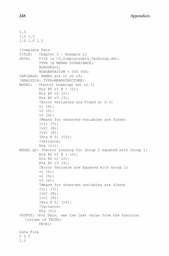
248 Appendices
1.31.0 1.31.0 1.0 1.3
!Complete DataTITLE: Chapter 3 - Example 2;DATA: FILE is C3_Completedata_TwoGroup.dat; TYPE IS MEANS COVARIANCE; NGROUPS=2; NOBSERVATION = 500 500;VARIABLE: NAMES are v1 v2 v3;!ANALYSIS: TYPE=MEANSTRUCTURE;MODEL: !Factor Loadings set to 1; Eta BY v1 @ 1 (1); Eta BY v2 (2); Eta BY v3 (3); !Error Variances are Fixed at 0.3; v1 (4); v2 (5); v3 (6); !Means for observed variables are fixed; [v1] (7); [v2] (8); [v3] (9); [Eta @ 0] (10); !Variance; Eta (11);MODEL g2: !Factor Loading for Group 2 equated with Group 1; Eta BY v1 @ 1 (1); Eta BY v2 (2); Eta BY v3 (3); !Error Variance are Equated with Group 1; v1 (4); v2 (5); v3 (6); !Means for observed variables are fixed; [v1] (7); [v2] (8); [v3] (9); [Eta @ 0] (10); !Variance; Eta (11)OUTPUT: !For Fmin, see the last value from the function !column of TECH5; TECH1;
Data File5 5 51.3
Y100315.indb 248 7/15/09 3:00:20 PM

Appendices 249
1.0 1.31.0 1.0 1.35 5 51.31.0 1.31.0 1.0 1.3
MPlus (3.3)
TITLE: Chapter 3 - Example 3;DATA: FILE is C3_Missingdata_TwoGroup.dat; TYPE IS MEANS COVARIANCE; NGROUPS=2; NOBSERVATION = 500 500;VARIABLE: NAMES are v1 v2 v3;!ANALYSIS: TYPE=MEANSTRUCTURE;MODEL: !Factor Loadings set to 1; Eta BY v1 @ 1 (1); Eta BY v2 (2); Eta BY v3 (3); !Error Variances are Fixed at 0.3; v1 (4); v2 (5); v3 (6); !Means for observed variables are fixed; [v1] (7); [v2] (8); [v3] (9); [Eta @ 0] (10); !Variance; Eta (11);MODEL g2: !Factor Loading for Group 2 equated with Group 1; !Factor Loading for v3 fixed at 0; !Eta BY v1 @ 1 (1); !Eta BY v2 (2); Eta BY v3 @ 0; !Error Variance are Equated with Group 1; !Error Variance for v3 fixed at 1.0; !v1 (4); !v2 (5); [email protected]; !Means for observed variables are fixed; !Mean for v3 fixed at 0; ![v1] (7); ![v2] (8); [v3 @ 0]; ![Eta @ 0] (10); !Variance; !Eta (11)
Y100315.indb 249 7/15/09 3:00:20 PM

250 Appendices
OUTPUT: !For Fmin, see the last value from the function !column of TECH5; TECH1;*Data file5 5 51.31.0 1.31.0 1.0 1.35 5 01.31.0 1.30 0 1
aMOS Syntax
' Example 3.1Module MainModule Sub Main() Dim Sem As New AmosEngine Try Sem.TextOutput() Sem.ModelMeansAndIntercepts() Sem.BeginGroup("Chapter3_complete data.xls', "Sheet1") 'Factor Loadings Sem.AStructure("v1 = (1)Eta1 + (1)ev1") Sem.AStructure("v2 = Eta1 + (1)ev2") Sem.AStructure("v3 = Eta1 + (1)ev3") 'Factor Means Sem.Mean("v1") Sem.Mean("v2") Sem.Mean("v3") Sem.FitModel() Finally Sem.Dispose() End Try End SubEnd Module
' Example 3.2#Region "Header"Imports SystemImports System.DiagnosticsImports Microsoft.VisualBasicImports AmosEngineLibImports AmosGraphics
Y100315.indb 250 7/15/09 3:00:20 PM

Appendices 251
Imports AmosEngineLib.AmosEngine.TMatrixIDImports PBayes#End RegionModule MainModule Sub Main() Dim Sem As New AmosEngine Try Sem.TextOutput() Sem.ModelMeansAndIntercepts() Sem.BeginGroup("Ch3_AMOS.xls", "Sheet1") Sem.GroupName("Group 1") 'Factor Loadings Sem.AStructure("v1 = (1)Eta1 + (1)err1_1") Sem.AStructure("v2 = (a1_1) Eta1 +(1)err2_1") Sem.AStructure("v3 = (a2_2) Eta1 + (1)err3_1") ‘Factor Variances Sem.Var("err1_1", "err1") Sem.Var("err2_1", "err2") Sem.Var("err3_1", "err3") Sem.Var("Eta1", "Eta") ‘Mean ‘Intercept Sem.Mean ("v1", "vm1") Sem.Mean ("v2", "vm2") Sem.Mean ("v3", "vm3") Sem.BeginGroup("Ch3_AMOS2.xls", "Sheet1") Sem.GroupName("Group 2") 'Factor Loadings Sem.AStructure("v1 = (1)Eta1 + (1)err1_2") Sem.AStructure("v2 = (a1_1) Eta1 + (1)err2_2") Sem.AStructure("v3 = (a2_2) Eta1 + (1)err3_2") 'Factor Variances Sem.Var("err1_2", "err1") Sem.Var("err2_2", "err2") Sem.Var("err3_2", "err3") Sem.Var("Eta1", "Eta") 'Mean 'Intercept Sem.Mean ("v1", "vm1") Sem.Mean ("v2", "vm2") Sem.Mean ("v3", "vm3")
Sem.FitAllModels
Y100315.indb 251 7/15/09 3:00:20 PM

252 Appendices
Finally Sem.Dispose() End Try End SubEnd Module
' Example 3.3#Region "Header"Imports SystemImports System.DiagnosticsImports Microsoft.VisualBasicImports AmosEngineLibImports AmosGraphicsImports AmosEngineLib.AmosEngine.TMatrixIDImports PBayes#End RegionModule MainModule Sub Main() Dim Sem As New AmosEngine Try Sem.TextOutput() Sem.ModelMeansAndIntercepts() Sem.BeginGroup("Ch3_AMOS.xls", "Sheet1") Sem.GroupName("Complete Group") 'Factor Loadings Sem.AStructure("v1 = (1)Eta1 + (1)err1_1") Sem.AStructure("v2 = (a1_1) Eta1 + (1)err2_1") Sem.AStructure("v3 = (a2_2) Eta1 + (1)err3_1") 'Factor Variances Sem.Var("err1_1", "err1") Sem.Var("err2_1", "err2") Sem.Var("err3_1", "err3") Sem.Var("Eta1", "Eta") 'Mean 'Intercept Sem.Mean ("v1", "vm1") Sem.Mean ("v2", "vm2") Sem.Mean ("v3", "vm3") Sem.BeginGroup("Ch3_AMOS_Missinggroup.xls", "Sheet1") Sem.GroupName("Missing Group") 'Factor Loadings Sem.AStructure("v1 = (1)Eta1 + (1)err1_2")
Y100315.indb 252 7/15/09 3:00:20 PM

Appendices 253
Sem.AStructure("v2 = (a1_1) Eta1 + (1)err2_2") Sem.AStructure("v3 = (0) Eta1 + (1)err3_2") 'Factor Variances Sem.Var("err1_2", "err1") Sem.Var("err2_2", "err2") Sem.Var("err3_2", "1") Sem.Var("Eta1", "Eta") 'Mean 'Intercept Sem.Mean ("v1", "vm1") Sem.Mean ("v2", "vm2") Sem.Mean ("v3", "0") Sem.FitAllModels Finally Sem.Dispose() End Try End SubEnd Module
Chapter 4 Appendix
liSrel Syntax
! SATORRA AND SARIS (1985) EXAMPLEDA NI=2 NO=123LAV1 V2CM1.00.25 1.0MO NY=2 NE=2 LY=ID PS=SY,FI TE=SY,FIFR PS(1,1) PS(2,2)pdOU ND=5
! Chapter 4: Satorra & Saris _Figure 4.6 ExampleLISRELDA NI=5 NO=1000LAX Y1 Y2 Y3 Y4CM1
Y100315.indb 253 7/15/09 3:00:20 PM

254 Appendices
0 10 0 10 0 0 10 0 0 0 1MO NY=5 NE=5 LY=ID PS=SY,FI BE=FU,FI TE=ZEVA 1.0 PS(1,1)VA 0.84 PS(2,2)VA 0.61 PS(3,3)VA 0.84 PS(4,4)VA 0.27 PS(5,5)VA 0.4 BE(2,1)VA 0.5 BE(3,1)VA 0.4 BE(4,1)VA 0.4 BE(5,2)VA 0.4 BE(5,3)VA 0.4 BE(5,4)VA 0.2 BE(3,2)OU ND=5 RS
! HANCOCK (2006) EXAMPLEDA NI=2 NO=123LAV1 V2CM10 1MO NY=2 NE=2 LY=FU,FI PS=SY,FI TE=SY,FIVA 1.0 PS(1,1) PS(2,2)VA 0.25 PS(1,2)VA .9354 LY(1,1) LY(2,2)VA .3 TE(1,1) TE(2,2)FR PS(1,1) PS(2,2)OU ND=5 RS SS
MPlus Syntax
!Complete DataTITLE: Chapter 4 - Satorra and Saris;DATA: FILE is C4_SatorraSaris.dat; TYPE IS COVARIANCE; NOBSERVATION = 123;VARIABLE: NAMES are v1 v2;MODEL: !Factor Loadings set to 1; Eta1 BY v1 @ 1; Eta2 BY v2@ 1; !Error Variances are Fixed at 0.3; v1-v2@0;
Y100315.indb 254 7/15/09 3:00:20 PM

Appendices 255
!Variance and Covariances; Eta1; Eta2; Eta1 with Eta2@0;OUTPUT: !For Fmin, see the last value from the function column of TECH5; TECH1;Data File1.00.25 1.00
MPlusTITLE: Chapter 4 - Satorra and Saris_Figure 4.6;DATA: FILE is C4_SatorraSaris2.dat; TYPE IS COVARIANCE; NOBSERVATION = 1000;VARIABLE: NAMES are X Y1 Y2 Y3 Y4;MODEL: !Variance and Covariances; [email protected]; [email protected]; [email protected]; [email protected]; [email protected]; !Beta; Y1 ON [email protected]; Y2 ON [email protected]; Y3 ON [email protected]; Y2 ON [email protected]; Y4 ON [email protected]; Y4 ON [email protected]; Y4 ON [email protected];OUTPUT: RESIDUAL TECH1;
Data File10 10 0 10 0 0 10 0 0 0 1
MPlusTITLE: Chapter 4 - Satorra and Saris;DATA: FILE is C4_Hancock.dat; TYPE IS COVARIANCE; NOBSERVATION = 123;VARIABLE: NAMES are v1 v2;MODEL: !Factor Loadings set to .9354; Eta1 BY v1 @ .9354;
Y100315.indb 255 7/15/09 3:00:20 PM

256 Appendices
Eta2 BY v2@ .9354; !Error Variances are Fixed at 0.3; [email protected]; !Variance and Covariances; [email protected] ; [email protected]; Eta1 with [email protected];OUTPUT: !For Fmin, see the last value from the function column of TECH5; RESIDUAL TECH1;
aMOS Syntax
Module MainModule Sub Main() Dim Sem As New AmosEngine Try Sem.TextOutput() Sem.BeginGroup("Chapter3_satorra_saris.xls", "Sheet1") 'Factor Loadings Sem.AStructure("v1 = (1)Eta1 + (1)ev1") Sem.AStructure("v2 = (1)Eta2 + (1)ev2") Sem.Var("Eta1") Sem.Var("Eta2") Sem.Var("ev1", "0") Sem.Var("ev2", "0") Sem.FitModel() Finally Sem.Dispose() End Try End SubEnd Module
#Region "Header"Imports SystemImports System.DiagnosticsImports Microsoft.VisualBasicImports AmosEngineLibImports AmosGraphicsImports AmosEngineLib.AmosEngine.TMatrixIDImports PBayes#End RegionModule MainModule Sub Main() Dim Sem As New AmosEngine Try
Y100315.indb 256 7/15/09 3:00:20 PM

Appendices 257
Sem.TextOutput() Sem.BeginGroup("Ch3_Satorra_saris_4.6.xls", "Sheet1") 'Factor Loadings Sem.AStructure("y1 = (.4)X + (1)u1") Sem.AStructure("y2 = (.5)X + (1)u2") Sem.AStructure("y3 = (.4)X + (1)u3") Sem.AStructure("y2 = (.2) y1 ") Sem.AStructure("y4 = (.4)y1 + (.4)y2 + (.4)y3 + (1)u4") 'Fixed Variances Sem.Var("X", "1.0") Sem.Var("u1", "0.84") Sem.Var("u2", "0.61") Sem.Var("u3", "0.84") Sem.Var("u4", "0.27") 'Fixed Regression Weights 'Sem.AStructure("y2<--y1") Sem.FitModel() Finally Sem.Dispose() End Try End SubEnd Module
#Region "Header"Imports SystemImports System.DiagnosticsImports Microsoft.VisualBasicImports AmosEngineLibImports AmosGraphicsImports AmosEngineLib.AmosEngine.TMatrixIDImports PBayes#End RegionModule MainModule Sub Main() Dim Sem As New AmosEngine Try Sem.ImpliedMoments Sem.TextOutput() Sem.BeginGroup("Ch3_Hancock.xls", "Sheet1") 'Factor Loadings Sem.AStructure("v1 = (.9354)Eta1 + (1)ev1")
Y100315.indb 257 7/15/09 3:00:20 PM
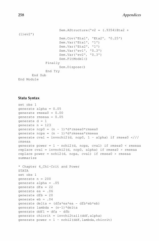
258 Appendices
Sem.AStructure("v2 = (.9354)Eta2 + (1)ev2") Sem.Cov("Eta1", "Eta2", "0.25") Sem.Var("Eta1", "1") Sem.Var("Eta2", "1") Sem.Var("ev1", "0.3") Sem.Var("ev2", "0.3") Sem.FitModel() Finally Sem.Dispose() End Try End SubEnd Module
Stata Syntax
set obs 1generate alpha = 0.05generate rmsea0 = 0.00generate rmseaa = 0.05generate d = 1generate n = 123generate ncp0 = (n - 1)*d*rmsea0*rmsea0generate ncpa = (n - 1)*d*rmseaa*rmseaagenerate cval = invnchi2(d, ncp0, 1 - alpha) if rmsea0 </// rmseaagenerate power = 1 - nchi2(d, ncpa, cval) if rmsea0 < rmseaareplace cval = invnchi2(d, ncp0, alpha) if rmsea0 > rmseaareplace power = nchi2(d, ncpa, cval) if rmsea0 > rmseaasummarize
* Chapter 4_Chi-Crit and PowerSTATAset obs 1generate n = 200generate alpha = .05generate dfa = 22generate ea = .06generate dfb = 20generate eb = .04generate delta = (dfa*ea*ea - dfb*eb*eb)generate lambda = (n-1)*deltagenerate ddf1 = dfa - dfbgenerate chicrit = invchi2tail(ddf,alpha)generate power = 1 - nchi2(ddf,lambda,chicrit)
Y100315.indb 258 7/15/09 3:00:20 PM

Appendices 259
SPSS Syntax
**********************************************************.*cval computed as invnchi2(d, ncp0, 1 - alpha) if *rmsea0<rmseaa.*OR invnchi2(d, ncp0, alpha) if rmsea0 > rmseaa.*Since invnchi2 function is not available in SPSS, compute *the.*inverse of noncentral chi-squared distribution in STATTAB.*http://odin.mdacc.tmc.edu/anonftp/*or G*Power* http://www.psycho.uni-duesseldorf.de/abteilungen/aap/*gpower3/***********************************************************.DATA LIST LIST/fit (A15) alpha rmsea0 rmseaa d n cval.
BEGIN DATA"close" 0.05 0.05 0.08 1 123 4.947754"not close" 0.05 0.05 0.01 1 123 0.005334"exact" 0.05 0.00 0.05 1 123 3.8141459END DATA.
COMPUTE ncp0 = (n-1)*d*rmsea0*rmsea0.COMPUTE ncpa = (n-1)*d*rmseaa*rmseaa.do if (rmsea0<rmseaa).Compute power = 1- NCDF.CHISQ(cval, d, ncpa).Else if (rmsea0>rmseaa). COMPUTE power = NCDF.CHISQ(cval, d, ncpa).end if.execute.
DATA LIST FREE / obs.BEGIN DATA.1END DATA.COMPUTE n = 200.COMPUTE alpha = 0.05.COMPUTE dfa = 22.COMPUTE ea = 0.06.COMPUTE dfb = 20.COMPUTE eb = 0.04.COMPUTE delta = (dfa*ea*ea - dfb*eb*eb).COMPUTE lambda = (n-1)*delta.
Y100315.indb 259 7/15/09 3:00:20 PM

260 Appendices
COMPUTE ddf = dfa - dfb.COMPUTE chicrit = IDF.CHISQ(1-alpha,ddf) .COMPUTE power = 1-NCDF.CHISQ(chicrit, ddf, lambda) .execute.
SaS Syntax
data maccallum;do obs=1;alpha=0.05;rmsea0=0.00;rmseaa=0.05;df=1;n=123;ncp0=(n-1)*df*rmsea0*rmsea0;ncpa=(n-1)*df*rmseaa*rmseaa;IF rmsea0<rmseaa THEN cval=cinv(1-alpha, df, ncp0);IF rmsea0<rmseaa THEN power=1- PROBCHI(cval,df,ncpa);IF rmsea0>rmseaa THEN cval=cinv(alpha, df, ncp0);IF rmsea0>rmseaa THEN power=PROBCHI(cval,df,ncpa);output;end;proc print data=maccallum;var n rmsea0 rmseaa cval power;run;
data chicrit;do obs=1;n=200;alpha=0.05;dfa = 22;ea = .06;dfb = 20;eb = .04;delta = (dfa*ea*ea - dfb*eb*eb);lambda = (n-1)*delta;ddf= dfa - dfb;chicrit = quantile('chisquare', 1-alpha, ddf);power=1-PROBCHI(chicrit,ddf,lambda);output;end;proc print data=chicrit;var n chicrit delta lambda power;run;
Y100315.indb 260 7/15/09 3:00:20 PM

Appendices 261
Chapter 5 Appendix
liSrel Syntax
! Example 5.1DA NI=2 NO=1000LAY1 Y2CM10 1ME0 0MO NY=2 NE=2 LY=FU,FI PS=SY,FI TE=SY,FI TY=FI AL=FIVA 1 LY(1,1) LY(2,2)VA 256 PS(1,1) PS(2,2)VA 64 PS(1,2)VA 100 TY(1) TY(2)OU RS ND=5
MPlus SyntaxTITLE: Chapter 5 - Example 1;DATA: FILE is Ch5_example1.dat; TYPE is MEANS COVARIANCE; NOBSERVATIONS = 1000;VARIABLE: NAMES are Y1 Y2;MODEL: !Factor Loadings set to 1; Eta1 BY Y1 @ 1; Eta2 BY Y2 @ 1; !Error variances are fixed; Y1 @ 0; Y2 @ 0; !Variances for Psi; Eta1 @ 256; Eta2 @ 256; Eta1 with Eta2 @ 64; !Means for observed variables are fixed; [Y1-Y2@0]; !Means for latent factors are fixed; [Eta1-Eta2@ 100];OUTPUT: RESIDUAL TECH1;
aMOS Syntax
#Region "Header"Imports System
Y100315.indb 261 7/15/09 3:00:20 PM

262 Appendices
Imports System.DiagnosticsImports Microsoft.VisualBasicImports AmosEngineLibImports AmosGraphicsImports AmosEngineLib.AmosEngine.TMatrixIDImports PBayes#End RegionModule MainModule Sub Main() Dim Sem As New AmosEngine Try Sem.ImpliedMoments Sem.ModelMeansAndIntercepts Sem.TextOutput() Sem.BeginGroup("Ch5_Example1.xls", "Sheet1") 'Factor Loadings Sem.AStructure("v1 = (1)Eta1 + (1)ev1") Sem.AStructure("v2 = (1)Eta2 + (1)ev2") Sem.Cov("Eta1", "Eta2", "64") Sem.Var("Eta1", "256") Sem.Var("Eta2", "256") Sem.Var("ev1", "0") Sem.Var("ev2", "0") Sem.Mean("Eta1", "100") Sem.Mean("Eta2", "100") Sem.FitModel() Finally Sem.Dispose() End Try End SubEnd Module
SaS Syntax
/* Selection syntax */PROC IML; LY = {1 0, 0 1}; PS = {256 64, 64 256}; TE = {0 0, 0 0}; TY = {100, 100}; W = {1, 0}; SIGMA = LY*PS*LY`+TE;
Y100315.indb 262 7/15/09 3:00:20 PM

Appendices 263
/*Mean of Selection Variable - Selection on Observed Variables*/ mus = w`*ty;
/*Variance of Selection Variable*/ vars = w`*sigma*w;
/*Standard Deviation of Selection Variable*/ sds = root(vars);/*This syntax calculates from 5% to 95% cutpoints*/do I = 0.05 to 1 by .05;
/*Mean and Variance in Selected Subsample (>= cutpoint)*/d=quantile('NORMAL',I);phis = PDF('NORMAL',trace(d));phiss = CDF('NORMAL',trace(d));xPHIs = I(1)-phiss;/*Mean of Selection Variance (Selected and Unselected Groups)*/
muss = mus + sds*phis*inv(xPHIs);musu = mus - sds*phis*inv(phiss);/*Variance of Selection Variance (Selected and Unselected Groups)*/varss = vars*(1 + (d*phis*inv(xPHIs)) -(phis*phis*inv(xPHIs)*inv(xPHIs)));varsu = vars*(1 - (d*phis*inv(phiss)) -
(phis*phis*inv(phiss)*inv(phiss)));
/*Omega (Selected and Unselected Groups)*/omegas = inv(vars)*(varss - vars)*inv(vars);omegau = inv(vars)*(varsu - vars)*inv(vars);
/*Sigma (Selected and Unselected Groups)*/sigmas = sigma + omegas*(sigma*(w*w`)*sigma);sigmau = sigma + omegau*(sigma*(w*w`)*sigma);
/*Kappa (Selected and Unselected Groups)*/ks = inv(vars)*(muss - mus);ku = inv(vars)*(musu - mus);
/*Means (Selected and Unselected Groups)*/muys = ty + sigma*w*ks;muyu = ty + sigma*w*ku;
print I;print sigmas;
Y100315.indb 263 7/15/09 3:00:20 PM

264 Appendices
print muys;print sigmau;print muyu;end;quit;
/* Selection in 3 parts *//*SPECIFY THE POPULATION MODEL*/PROC IML;ly = {1 0,0 1};ps = {256 64,64 256};te = {0 0,0 0};ty = {100, 100};/*Specify Weight Matrix*/w = {1, 0};sigma = ly*ps*ly` + te;/*Mean of Selection Variable - Selection on Observed Variables*/mus = w`*ty;/*Variance of Selection Variable*/vars = w`*sigma*w;/*Standard Deviation of Selection Variable*/sds = root(vars);/*To divide population in three we must define two cutpoints using z scores*/;/*Ranges are thus z=infinity to -0.97, -0.97 to +0.97, and +0.97 to +infinity*/;z1 = PROBIT(0.333333);z2 = PROBIT(0.666667);phis1 = PDF('NORMAL',trace(z1));phis2 = PDF('NORMAL',trace(z2));phiss1 = CDF('NORMAL',trace(z1));phiss2 = CDF('NORMAL',trace(z2));/*Mean of Selection Variable in Selected Portion of Sample*/m3 = mus - sds*(phis2-phis1)*inv(phiss2-phiss1);/*Variance of Selection Variable in Selected Portion of Sample*/vars3 = vars*(1 - ((z2*phis2-z1*phis1)*inv(phiss2-phiss1)) - (phis2-phis1)*(phis2-phis1)*inv(phiss2-phiss1)*inv(phiss2-phiss1));/*Omega (Selected)*/omegas = inv(vars)*(vars3 - vars)*inv(vars);/*Kappa (Selected)*/ks =inv(vars)*(m3 - mus);/*Sigma (Selected)*/
Y100315.indb 264 7/15/09 3:00:20 PM
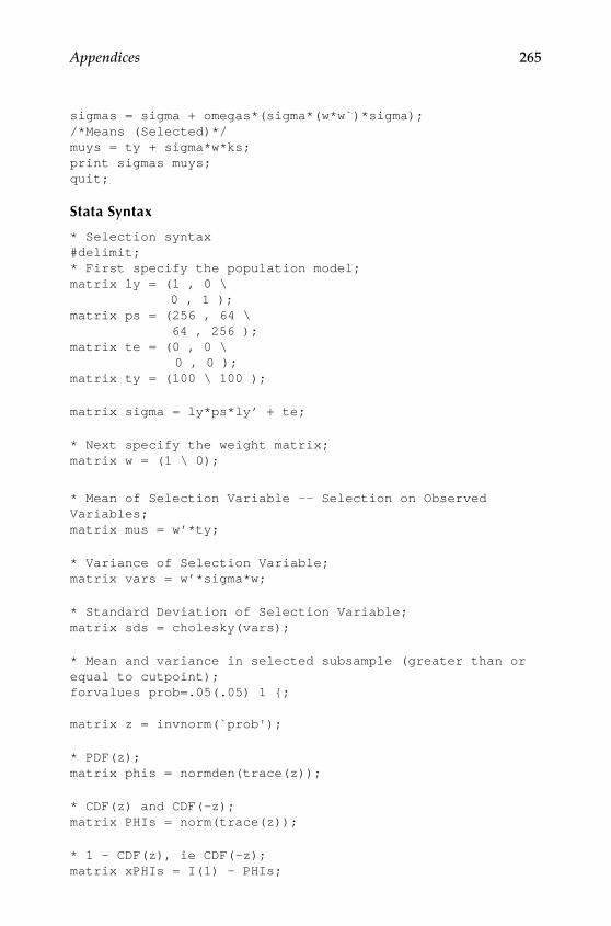
Appendices 265
sigmas = sigma + omegas*(sigma*(w*w`)*sigma);/*Means (Selected)*/muys = ty + sigma*w*ks;print sigmas muys;quit;
Stata Syntax
* Selection syntax#delimit;* First specify the population model;matrix ly = (1 , 0 \ 0 , 1 );matrix ps = (256 , 64 \ 64 , 256 );matrix te = (0 , 0 \ 0 , 0 );matrix ty = (100 \ 100 );
matrix sigma = ly*ps*ly’ + te;
* Next specify the weight matrix;matrix w = (1 \ 0);
* Mean of Selection Variable -- Selection on Observed Variables;matrix mus = w’*ty;
* Variance of Selection Variable;matrix vars = w’*sigma*w;
* Standard Deviation of Selection Variable;matrix sds = cholesky(vars);
* Mean and variance in selected subsample (greater than or equal to cutpoint);forvalues prob=.05(.05) 1 {;
matrix z = invnorm(`prob');
* PDF(z);matrix phis = normden(trace(z));
* CDF(z) and CDF(-z);matrix PHIs = norm(trace(z));
* 1 - CDF(z), ie CDF(-z);matrix xPHIs = I(1) - PHIs;
Y100315.indb 265 7/15/09 3:00:21 PM

266 Appendices
* Mean of Selection Variable in Selected and Unselected Portions of Sample;matrix muss = mus + sds*phis*inv(xPHIs);matrix musu = mus - sds*phis*inv(PHIs);
* Variance of Selection Variable in Selected and Unselected Portions of Sample;matrix varss = vars*(1 + (z*phis*inv(xPHIs)) - (phis*phis*inv(xPHIs)*inv(xPHIs)));matrix varsu = vars*(1 - (z*phis*inv(PHIs)) - (phis*phis*inv(PHIs)*inv(PHIs)));* Standard Deviation of Selection Variable in Selected and Unselected Portions of Sample;matrix sdss = cholesky(varss);matrix sdsu = cholesky(varsu);
* Calculate Omega (Selected and Unselected);matrix omegas = inv(vars)*(varss - vars)*inv(vars);matrix omegau = inv(vars)*(varsu - vars)*inv(vars);
* Calculate Sigma (Selected and Unselected);matrix sigmas = sigma + omegas*(sigma*(w*w’)*sigma);matrix sigmau = sigma + omegau*(sigma*(w*w’)*sigma);
* Calculate Kappa (Selected and Unselected);matrix ks = inv(vars)*(muss - mus);matrix ku = inv(vars)*(musu - mus);
* Calculate Muy (Selected and Unselected);matrix muys =ty + sigma*w*ks;matrix muyu = ty + sigma*w*ku;
matrix list PHIs;matrix list sigmas;matrix list muys;matrix list sigmau;matrix list muyu;matrix list z;
};
* Can Use This Syntax to Generate Observations to Check Work;*corr2data x y , n(1000) m(ty) cov(sigma);*generate s = x;
*SPECIFY THE POPULATION MODEL;matrix ly = (1 , 0\ 0 , 1);
Y100315.indb 266 7/15/09 3:00:21 PM

Appendices 267
matrix ps = (256 , 64 \ 64, 256 );matrix te = (0, 0 \ 0, 0);matrix ty =(100\100);matrix sigma = ly*ps*ly’ + te;
* SPECIFY WEIGHT MATRIX;matrix w = (1\ 0);* MEAN OF SELECTION VARAIBLE;matrix mus = w’*ty;
* VARIANCE OF SELECTION VARIABLE;matrix vars = w'*sigma*w;* STANDARD DEVIATION OF SELECTION VARIABLE;matrix sds = cholesky(vars);
* TO DIVIDE POPULATION IN THREE WE MUST DEFINE TWO CUTPOINTS USING Z-SCORES;* Ranges are thus z=-infinity to -0.97, -0.97 to +0.97, and +0.97 to +infinity;
matrix z1 = invnorm(0.333333);matrix z2 = invnorm(0.666667);
*PDF(z);matrix phis1 = normden(trace(z1));matrix PHIs1 = norm(trace(z1));
*CDF(z);matrix phis2 = normden(trace(z2));matrix PHIs2 = norm(trace(z2));
*MEAN OF SELECTION VARIABLE IN SELECTED PORTION OF SAMPLE;matrix m3 = mus - sds*(phis2-phis1)*inv(PHIs2-PHIs1);
*VARIANCE OF SELECTION VARIABLE IN SELECTED PORTION OF SAMPLE;matrix vars3 = vars*(1 - ((z2*phis2-z1*phis1)*inv(PHIs2-PHIs1)) - (phis2-phis1)*(phis2-phis1)*inv(PHIs2-PHIs1)*inv(PHIs2-PHIs1));
*STANDARD DEVIATION OF SELECTION VARIABLE IN SELECTED PORTION OF SAMPLE;matrix sds3 = cholesky(vars3);
* OMEGA (Selected);matrix omegas = inv(vars)*(vars3 - vars)*inv(vars);
Y100315.indb 267 7/15/09 3:00:21 PM

268 Appendices
* KAPPA (Selected and Unselected);matrix ks = inv(vars)*(m3 - mus);* SIGMA (Selected);matrix sigmas = sigma + omegas*(sigma*(w*w')*sigma);
* MUY (Selected);matrix muys = ty + sigma*w*ks;
matrix list sigmas;matrix list muys;
SPSS Syntax
* Selection syntax.
Input program.Loop I = 0.05 to 1 by (.05). End case.End Loop.End File.End Input Program.Execute.
COMPUTE d = IDF.NORMAL(I, 0,1).COMPUTE phis = PDF.NORMAL(d ,0,1).Compute phiss = CDFNORM(d).execute.
matrix.
Get D/variables = d.
Get PHIS/variables = phis.
Get PHISS/variables = phiss.
compute ly = {1,0;0,1}.
compute ps = {256, 64;
Y100315.indb 268 7/15/09 3:00:21 PM

Appendices 269
64, 256}
compute te = {0,0;0,0}
compute ty = {100;100}
compute w = {1;0}
compute sigma = ly * ps * t(ly) + te.
* Mean of Selection variable -- Selection on Observed Variables.compute mus = t(w)*ty.
* Variance of Selection Variable.compute vars = t(w)*sigma*w.
* Standard Deviation of Selection Variable.compute sds = chol(vars).
loop i=1 to 19.compute missamt = 5*i.compute xPHIs = ident(1) - phiss.
compute muss = mus + sds*phis(i)*inv(xphis(i)).compute musu = mus - sds*phis(i)*inv(phiss(i)).
compute varss = vars *(1 + (d(i)*phis(i)*inv(xPHIs(i))) - (phis(i)*phis(i)*inv(xPHIs(i))*inv(xPHIs(i)))).compute varsu = vars *(1 - (d(i)*phis(i)*inv(phiss(i))) - (phis(i)*phis(i)*inv(phiss(i))*inv(phiss(i)))).
compute omegas = inv(vars)*(varss - vars)*inv(vars).compute omegau = inv(vars)*(varsu - vars)*inv(vars).
compute sigmas = sigma + omegas* (sigma*(w*t(w))*sigma).compute sigmau = sigma + omegau* (sigma*(w*t(w))*sigma).
compute ks = inv(vars)*(muss - mus).compute ku = inv(vars)*(musu - mus).
Y100315.indb 269 7/15/09 3:00:21 PM

270 Appendices
compute muys = ty + sigma*w*ks.compute muyu = ty + sigma*w*ku.
print missamt.print sigmas.print muys.print sigmau.print muyu.end loop.end matrix.execute.
* Selection Syntax in 3 Parts.DATA LIST FREE / I1 I2.BEGIN DATA.0.3333330.666667END DATA.
COMPUTE z1 = IDF.NORMAL(I1, 0, 1).COMPUTE z2 = IDF.NORMAL(I2, 0, 1).COMPUTE phis1 = PDF.NORMAL(z1 ,0,1).COMPUTE phis2 = PDF.NORMAL(z2 ,0,1).Compute phiss1 = CDFNORM(z1).Compute phiss2 = CDFNORM(z2).execute.
matrix.
Get z1/variables = z1.
Get z2/variables = z2.
Get phis1/variables = phis1.
Get phis2/variables = phis2.
Get phiss1/variables = phiss1.
Get phiss2/variables = phiss2.
compute ly = {
Y100315.indb 270 7/15/09 3:00:21 PM

Appendices 271
1,0;0,1}.
compute ps = {256, 64;64, 256}
compute te = {0,0;0,0}
compute ty = {100;100}compute w = {1,0}
compute sigma = ly * ps * t(ly) + te.
* Mean of Selection variable -- Selection on Observed Variables.compute mus = w*ty.* Variance of Selection Variable.compute vars = w*sigma*t(w).
* Standard Deviation of Selection Variable.compute sds = chol(vars).
*To Divide Population in Three we must Define Two Cutpoints Using Z-Scores;*Ranges are thus z=-infinity to -0.97, -0.97 to +0.97, and +0.97 to +infinity;
compute m3 = mus - sds*(phis2-phis1)*inv(phiss2-phiss1).
compute vars3 = vars *(1 - ((z2*phis2 - z1*phis1)*inv(phiss2-phiss1)) - (phis2-phis1)*(phis2-phis1)*inv(phiss2-phiss1)*inv(phiss2-phiss1)).
compute omegas = inv(vars)*(vars3 - vars)*inv(vars).
compute sigmas = sigma + omegas* (sigma*(t(w)*w)*sigma).
compute ks = inv(vars)*(m3 - mus).
compute mues = ks*ps*t(ly)*t(w).
compute tys = ty + ly*mues.
Y100315.indb 271 7/15/09 3:00:21 PM

272 Appendices
print sigmas.print tys.end matrix.execute.
Chapter 6 – appendix
liSrel Syntax
! Complete Data (Constrained Covariance)da ni=2 no=10000 ng=2lax ycm1.0000.100 1.000me1.0 1.2mo ny=2 ne=2 ly=fu,fi ps=sy,fr te=sy,fi ty=fi al=frva 1.0 ly(1,1) ly(2,2)ou nd=5
da ni=2 no=10000 ng=2lax ycm1.0000.100 1.000me1.0 1.2mo ny=2 ne=2 ly=in ps=in te=in ty=in al=inou nd=5
Example 2: 2 Group Missing DataLISREL - EXAMPLE 2! Complete Data (Constrained Covariance)da ni=2 no=10000 ng=2lax ycm1.0000.100 1.000me1.0 1.2mo ny=2 ne=2 ly=fu,fi ps=sy,fr te=sy,fi ty=fi al=frva 1.0 ly(1,1) ly(2,2)ou nd=5
Y100315.indb 272 7/15/09 3:00:21 PM

Appendices 273
!Group 2da ni=2 no=10000 ng=2lax ycm1.0000 1.000me1.0 0mo ny=2 ne=2 ly=fu,fi ps=in te=sy,fi ty=fi al=fiva 1.0 ly(1,1)va 1.0 te(2,2)eq al(1,1) al(1)ou nd=5Example 4LISREL! Complete Data Group - Constrained Covariance Modelda ni=2 no=9500 ng=2lax ycm!Effect size ! Small Medium Large1.000 ! 1.000 1.000 1.0000.100 1.000 ! 0.100 1.000 0.243 1.000 0.371 1.000me1 1.2mo ny=2 ne=2 ly=fu,fi ps=sy,fr te=sy,fi ty=fi al=frva 1.0 ly(1,1) ly(2,2)fi ps(1,2)ou nd=5
! 5% Missing Data Group - Constrained Covariance Modelda ni=2 no=500lax ycm10 1me1 0mo ny=2 ne=2 ly=fu,fi ps=in te=sy,fi ty=fi al=frva 1.0 ly(1,1)va 1.0 te(2,2)eq al(1,1) al(1)fi al(2)ou nd=5
Y100315.indb 273 7/15/09 3:00:21 PM

274 Appendices
MPlus Syntax
MPlus - Example 1!Complete DataTITLE: Chapter 6 - Example 1;DATA: FILE is C6_Completedata_TwoGroup.dat; TYPE IS MEANS COVARIANCE; NGROUPS=2; NOBSERVATION = 10000 10000;VARIABLE: NAMES are p1 p2;ANALYSIS: TYPE=MEANSTRUCTURE;MODEL: !Factor Loadings set to 1; Eta1 BY p1 @ 1.0 (1); Eta2 BY p2 @ 1.0 (2); !Error Variances are Fixed; p1 @ 0 (3); p2 @ 0 (4); !Means for observed variables are fixed; [p1] (5); [p2] (6); [Eta1@0] (7); [Eta2@0] (8); !Variance; Eta1 (9) Eta2 (10); Eta1 with Eta2 (11);OUTPUT: !For Fmin, see the last value from the function column of TECH5; TECH1;
MPlus - Example 2TITLE: Chapter 6 - Example 2;DATA: FILE is C6_Missingdata_TwoGroup.dat; TYPE IS MEANS COVARIANCE; NGROUPS=2; NOBSERVATION = 10000 10000;VARIABLE: NAMES are p1 p2;ANALYSIS: TYPE=MEANSTRUCTURE;MODEL: !Factor Loadings set to 1; Eta1 BY p1 @ 1.0 (1); Eta2 BY p2 @ 1.0 ; !Error Variances are Fixed; p1 @ 0 (2); p2 @ 0 (3); !Means for observed variables are fixed; [p1] (4); [p2]; [Eta1@0] (5);
Y100315.indb 274 7/15/09 3:00:21 PM

Appendices 275
[Eta2@0] (6); !Variance; Eta1 (7) Eta2 (8); Eta1 with Eta2 (9);Model G2: Eta2 BY p2 @ 0; p2 @ 1; [p2@0]OUTPUT: !For Fmin, see the last value from the function column of TECH5; RESIDUAL TECH1;
TITLE: Chapter 6 - Example 3;DATA: FILE is C6_Missingdata_ConstrainCovariance.dat; TYPE IS MEANS COVARIANCE; NGROUPS=2; NOBSERVATION = 9500 500;VARIABLE: NAMES are p1 p2;ANALYSIS: TYPE=MEANSTRUCTURE;MODEL: !Factor Loadings set to 1; Eta1 BY p1 @ 1.0 (1); Eta2 BY p2 @ 1.0 ; !Error Variances are Fixed; p1 @ 0 (2); p2 @ 0 (3); !Means for observed variables are fixed; [p1] (4); [p2]; [Eta1@0] (5); [Eta2@0] (6); !Variance; Eta1 (7) Eta2 (8); Eta1 with Eta2 @0(9);Model G2: Eta2 BY p2 @ 0; p2 @ 1; [p2@0]OUTPUT: !For Fmin, see the last value from the function column of TECH5; RESIDUAL TECH1;
aMOS Syntax
Module MainModule Sub Main() Dim Sem As New AmosEngine Try
Sem.TextOutput()
Y100315.indb 275 7/15/09 3:00:21 PM

276 Appendices
Sem.ModelMeansAndIntercepts() Sem.BeginGroup("Ex1_Completedata.xls", "Sheet1") Sem.GroupName("Group 1") 'Factor Loadings Sem.AStructure("v1 = (1)Eta1 + (1)err1_1") Sem.AStructure("v2 = (1) Eta2 + (1)err2_1") 'Factor Variances Sem.Var("err1_1", "0") Sem.Var("err2_1", "0") Sem.Var("Eta1", "ps1") Sem.Var("Eta2", "ps2") Sem.Cov("Eta1", "Eta2", "ps3") 'Mean 'Intercept Sem.Mean ("v1") Sem.Mean ("v2") Sem.Mean ("Eta1","0") Sem.Mean ("Eta1","0") Sem.BeginGroup("Ex1_Completedata.xls", "Sheet1") Sem.GroupName("Group 2") 'Factor Loadings Sem.AStructure("v1 = (1)Eta1 + (1)err1_1") Sem.AStructure("v2 = (1) Eta2 + (1)err2_1") 'Factor Variances Sem.Var("err1_1", "0") Sem.Var("err2_1", "0") Sem.Var("Eta1", "ps1") Sem.Var("Eta2", "ps2") Sem.Cov("Eta1", "Eta2", "ps3") 'Mean 'Intercept Sem.Mean ("v1", "v1") Sem.Mean ("v2", "v2") Sem.Mean ("Eta1","0") Sem.Mean ("Eta1","0") Sem.FitAllModels Finally Sem.Dispose() End Try End Sub
AMOS - Example 2
Y100315.indb 276 7/15/09 3:00:21 PM

Appendices 277
#Region "Header"Imports SystemImports System.DiagnosticsImports Microsoft.VisualBasicImports AmosEngineLibImports AmosGraphicsImports AmosEngineLib.AmosEngine.TMatrixIDImports PBayes#End RegionModule MainModule Sub Main() Dim Sem As New AmosEngine Try Sem.TextOutput() Sem.ModelMeansAndIntercepts() Sem.BeginGroup("Ex2_Completedata.xls", "Sheet1") Sem.GroupName("Group 1") 'Factor Loadings Sem.AStructure("v1 = (1)Eta1 + (1)err1_1") Sem.AStructure("v2 = (1) Eta2 + (1)err2_1") 'Factor Variances Sem.Var("err1_1", "0") Sem.Var("err2_1", "0") Sem.Var("Eta1", "ps1") Sem.Var("Eta2", "ps2") Sem.Cov("Eta1", "Eta2", "ps3") 'Mean 'Intercept Sem.Mean ("v1", "v1") Sem.Mean ("v2") Sem.Mean ("Eta1","0") Sem.Mean ("Eta2","0") Sem.BeginGroup("Ex2_Missingdata.xls", "Sheet1") Sem.GroupName("Group 2") 'Factor Loadings Sem.AStructure("v1 = (1)Eta1 + (1)err1_1") Sem.AStructure("v2 = (0) Eta2 + (1)err2_1") 'Sem.Var ("v2<--Eta2", "0") 'Factor Variances Sem.Var("err1_1", "0") Sem.Var("err2_1", "1") Sem.Var("Eta1", "ps1")
Y100315.indb 277 7/15/09 3:00:21 PM

278 Appendices
Sem.Var("Eta2", "ps2") Sem.Cov("Eta1", "Eta2", "ps3") 'Mean 'Intercept Sem.Mean ("v1", "v1") Sem.Mean ("v2", "0") Sem.Mean ("Eta1","0") Sem.Mean ("Eta2","0") Sem.FitAllModels Finally Sem.Dispose() End Try End SubEnd Module#Region "Header"Imports SystemImports System.DiagnosticsImports Microsoft.VisualBasicImports AmosEngineLibImports AmosGraphicsImports AmosEngineLib.AmosEngine.TMatrixIDImports PBayes#End RegionModule MainModule Sub Main() Dim Sem As New AmosEngine Try Sem.TextOutput() Sem.ModelMeansAndIntercepts() Sem.BeginGroup("Ex3_Completedata.xls", "Sheet1") Sem.GroupName("Group 1") 'Factor Loadings Sem.AStructure("v1 = (1)Eta1 + (1)err1_1") Sem.AStructure("v2 = (1) Eta2 + (1)err2_1") 'Factor Variances Sem.Var("err1_1", "0") Sem.Var("err2_1", "0") Sem.Var("Eta1", "ps1") Sem.Var("Eta2", "ps2") Sem.Cov("Eta1", "Eta2", "0") 'Mean 'Intercept Sem.Mean ("v1", "v1") Sem.Mean ("v2") Sem.Mean ("Eta1","0") Sem.Mean ("Eta2","0")
Y100315.indb 278 7/15/09 3:00:21 PM

Appendices 279
Sem.BeginGroup("Ex3_Missingdata.xls", "Sheet1") Sem.GroupName("Group 2") 'Factor Loadings Sem.AStructure("v1 = (1)Eta1 + (1)err1_1") Sem.AStructure("v2 = (0) Eta2 + (1)err2_1") 'Sem.Var ("v2<--Eta2", "0") 'Factor Variances Sem.Var("err1_1", "0") Sem.Var("err2_1", "1") Sem.Var("Eta1", "ps1") Sem.Var("Eta2", "ps2") Sem.Cov("Eta1", "Eta2", "0") 'Mean 'Intercept Sem.Mean ("v1", "v1") Sem.Mean ("v2", "0") Sem.Mean ("Eta1","0") Sem.Mean ("Eta2","0") Sem.FitAllModels Finally Sem.Dispose() End Try End SubEnd Module
Stata Syntax
STATA - Example 3: Selection Syntax* Specify the population model;matrix ly = (1 , 0 \ 0 , 1 );* Replace Correlations with .243 and .371 for Moderate & Large Effect Sizes;matrix ps = (1.000 , 0.100 \ 0.100 , 1.000 );matrix te = (0 , 0 \ 0 , 0 );matrix ty = (1.0 \ 1.2 );matrix sigma = ly*ps*ly' + te;* Specify weight matrix;matrix w = (1 \ 0); * Missing data depend only on values of x;* Mean of Selection Variable - Selection on Observed Variables;matrix mus = w'*ty;* Variance of Selection Variable;matrix vars = w'*sigma*w;* Standard Deviation of Selection Variable;matrix sds = cholesky(vars);
Y100315.indb 279 7/15/09 3:00:21 PM

280 Appendices
* Mean and variance in selected subpopulation >= cutpoint, c);* This syntax calculates from 5% to 95% cutpoints;forvalues prob=.05(.05) 1 {;matrix z = invnorm(`prob');matrix phis = normalden(trace(z)); * PDF(z);matrix PHIs = normal(trace(z)); * CDF(z) and CDF(-z);matrix xPHIs = I(1) - PHIs; * 1 - CDF(z), ie CDF(-z);* Mean of Selection Variable (Selected and Unselected Subpopulations);matrix muss = mus + sds*phis*inv(xPHIs);matrix musu = mus - sds*phis*inv(PHIs);* Variance of Selection Variable (Selected and Unselected Subpopulations);matrix varss = vars*(1 + (z*phis*inv(xPHIs)) - (phis*phis*inv(xPHIs)*inv(xPHIs)));matrix varsu = vars*(1 - (z*phis*inv(PHIs)) - (phis*phis*inv(PHIs)*inv(PHIs)));* Omega (Selected and Unselected);matrix omegas = inv(vars)*(varss - vars)*inv(vars);matrix omegau = inv(vars)*(varsu - vars)*inv(vars);* Sigma (Selected and Unselected);matrix sigmas = sigma + omegas*(sigma*(w*w')*sigma);matrix sigmau = sigma + omegau*(sigma*(w*w')*sigma);* Kappa (Selected and Unselected);matrix ks = inv(vars)*(muss - mus);matrix ku = inv(vars)*(musu - mus);* Muy (Selected and Unselected);matrix muys =ty + sigma*w*ks;matrix muyu = ty + sigma*w*ku;matrix list PHIs;matrix list sigmas;matrix list muys;matrix list sigmau;matrix list muyu; };
#delimit;set more off;set obs 20;gen FMin0 = 0.01005; *0% missing data;gen FMin1 = 0.00955; *MCAR with 5% missing;gen FMin2 = 0.00774; *MAR with 5% missing;gen n = 50*_n;gen ncp0 = (n-1)*FMin0;gen ncp1 = (n-1)*FMin1;gen ncp2 = (n-1)*FMin2;gen df1 = 1;gen alpha = 0.05;
Y100315.indb 280 7/15/09 3:00:21 PM

Appendices 281
gen chicrit1 = invchi2tail(df1, alpha);gen power0 = 1- nchi2(df1,ncp0,chicrit1);gen power1 = 1- nchi2(df1,ncp1,chicrit1);gen power2 = 1- nchi2(df1,ncp2,chicrit1);list n ncp0 power0 ncp1 power1 ncp2 power2 , noobs clean table;
#delimit;set more off;set obs 10;generate df = _n;generate alpha = 0.05;generate power =0.80;gen chicrit = invchi2tail(df, alpha);gen ncp = invnchi2(df,chicrit,power);gen fmin0 = 0.01005;gen fmin1 = 0.00955;gen fmin2 = 0.00774;gen n0=ncp/fmin0;gen n1=ncp/fmin1;gen n2=ncp/fmin2;list df ncp n0 n1 n2, noobs clean table;
SaS Syntax
SAS: Example 3-Selection syntax.PROC IML; LY = {1 0, 0 1};/*Replace Correlations with .3 and .5 for Moderate and Large Effect Sizes*/ PS = {1 .10, .10 1}; TE = {0 0, 0 0}; TY = {1.0, 1.2}; W = {1, 0}; SIGMA = LY*PS*LY`+TE;
/*Mean of Selection Variable - Selection on Observed Variables*/ mus = w`*ty;
/*Variance of Selection Variable*/ vars = w`*sigma*w;
Y100315.indb 281 7/15/09 3:00:21 PM

282 Appendices
/*Standard Deviation of Selection Variable*/ sds = root(vars);/*This syntax calculates from 5% to 95% cutpoints*/do I = 0.05 to 1 by .05;
/*Mean and Variance in Selected Subsample (>= cutpoint)*/d=quantile('NORMAL',I);phis = PDF('NORMAL',trace(d));phiss = CDF('NORMAL',trace(d));xPHIs = I(1)-phiss;/*Mean of Selection Variance (Selected and Unselected Groups)*/
muss = mus + sds*phis*inv(xPHIs);musu = mus - sds*phis*inv(phiss);
/*Variance of Selection Variance (Selected and Unselected Groups)*/varss = vars*(1 + (d*phis*inv(xPHIs)) -(phis*phis*inv(xPHIs)*inv(xPHIs)));varsu = vars*(1 - (d*phis*inv(phiss)) -(phis*phis*inv(phiss)*inv(phiss)));
/*Omega (Selected and Unselected Groups)*/omegas = inv(vars)*(varss - vars)*inv(vars);omegau = inv(vars)*(varsu - vars)*inv(vars);
/*Sigma (Selected and Unselected Groups)*/sigmas = sigma + omegas*(sigma*(w`*w)*sigma);sigmau = sigma + omegau*(sigma*(w`*w)*sigma);
/*Kappa (Selected and Unselected Groups)*/ks = inv(vars)*(muss - mus);ku = inv(vars)*(musu - mus);
/*Means (Selected and Unselected Groups)*/muys = ty + sigma*w*ks;muyu = ty + sigma*w*ku;
print I;print sigmas;print muys;print sigmau;print muyu;end;quit;
Example 5: Power for a Given NCP, DF, Alpha
Y100315.indb 282 7/15/09 3:00:21 PM

Appendices 283
SASData power;Do obs = 1 to 20;FMin0 = 0.01005; *0% missing data;FMin1 = 0.00955; *MCAR with 5% missing;FMin2 = 0.00774; *MAR with 5% missing;n = 50*obs;*n = 200;ncp0 = (n-1)*FMin0;ncp1 = (n-1)*FMin1;ncp2 = (n-1)*FMin2;df = 1;alpha = 0.05;chicrit = quantile('chisquare',1-alpha, 1);;power0 = 1- CDF('CHISQUARE', chicrit,df,ncp0);power1 = 1- CDF('CHISQUARE', chicrit,df,ncp1);power2 = 1- CDF('CHISQUARE', chicrit,df,ncp2);Output;End;Proc Print;Var n ncp0 power0 ncp1 power1 ncp2 power2;Run;
Example 6: NCP and Sample Size for a Given DF, Alpha, PowerSASDATA ncp;Do df = 1 to 10; alpha = 0.05; power = 0.80; chicrit = quantile('chisquare',1-alpha, df); ncp = CINV(power, df, chicrit); fmin0 = 0.01005; fmin1 = 0.00955; fmin2 = 0.00774; n0=ncp/fmin0; n1=ncp/fmin1; n2=ncp/fmin2;Output;End;Proc Print data=ncp; Var df chicrit ncp n0 n1 n2;Run;
SPSS Syntax
SPSS Selection syntax: Example 3Input program.
Y100315.indb 283 7/15/09 3:00:22 PM

284 Appendices
Loop I = 0.05 to 1 by (.05). End case.End Loop.End File.End Input Program.Execute.
COMPUTE d = IDF.NORMAL(I, 0,1).COMPUTE phis = PDF.NORMAL(d ,0,1).Compute phiss = CDFNORM(d).execute.
matrix.
Get D/variables = d.Get PHIS/variables = phis.
Get PHISS/variables = phiss.
compute ly = {1,0;0,1}.
*Replace Correlation with .3 and .5 for Moderate and Large Effect Sizes.compute ps = {1.0, 0.1;0.1, 1.0}
compute te = {0,0;0,0}
compute ty = {1.0;1.2}
compute w = {1;0}
compute sigma = ly * ps * t(ly) + te.
* Mean of Selection variable -- Selection on Observed Variables.
Y100315.indb 284 7/15/09 3:00:22 PM

Appendices 285
compute mus = t(w)*ty.
* Variance of Selection Variable.compute vars = t(w)*sigma*w.
* Standard Deviation of Selection Variable.compute sds = chol(vars).
loop i=1 to 19.compute missamt = 5*i.compute xPHIs = ident(1) - phiss.
compute muss = mus + sds*phis(i)*inv(xphis(i)).compute musu = mus - sds*phis(i)*inv(phiss(i)).compute varss = vars *(1 + (d(i)*phis(i)*inv(xPHIs(i))) - (phis(i)*phis(i)*inv(xPHIs(i))*inv(xPHIs(i)))).compute varsu = vars *(1 - (d(i)*phis(i)*inv(phiss(i))) - (phis(i)*phis(i)*inv(phiss(i))*inv(phiss(i)))).
compute omegas = inv(vars)*(varss - vars)*inv(vars).compute omegau = inv(vars)*(varsu - vars)*inv(vars).
compute sigmas = sigma + omegas* (sigma*( w*t(w))*sigma).compute sigmau = sigma + omegau* (sigma*( w*t(w))*sigma).
compute ks = inv(vars)*(muss - mus).compute ku = inv(vars)*(musu - mus).
compute muys = ty + sigma*w*ks.compute muyu = ty + sigma*w*ks.
print missamt.print sigmas.print muys.print sigmau.print muyu.end loop.end matrix.execute.
DATA LIST FREE / obs.BEGIN DATA.1 2 3 4 5 6 7 8 9 10 11 12 13 14 15 16 17 18 19 20END DATA.
Compute FMin0 = 0.01005.Compute FMin1 = 0.00955.
Y100315.indb 285 7/15/09 3:00:22 PM

286 Appendices
Compute FMin2 = 0.00774.compute n = 50*obs.Compute ncp0 = (n-1)*FMin0.Compute ncp1 = (n-1)*FMin1.Compute ncp2 = (n-1)*FMin2.compute df = 1.compute alpha = 0.05.Compute chicrit = IDF.CHISQ(1-alpha,df) .Compute power0 = 1-NCDF.CHISQ(chicrit, df, ncp0) .Compute power1 = 1-NCDF.CHISQ(chicrit, df, ncp1) .Compute power2 = 1-NCDF.CHISQ(chicrit, df, ncp2) .execute.
SPSSDATA LIST FREE / obs.BEGIN DATA.1 2 3 4 5 6 7 8 9 10END DATA.
Compute df = obs.Compute alpha = 0.05.Compute power = 0.80.Compute chicrit = IDF.CHISQ(1-alpha,df) .*Get NCP value using G*Power.
Compute fmin0 = 0.01005.Compute fmin1 = 0.00955.Compute fmin2 = 0.00774.Compute n0=ncp/fmin0.Compute n1=ncp/fmin1.Compute n2=ncp/fmin2.Execute.list df chicrit ncp n0 n1 n2.execute.
Chapter 7 Appendix
SAS
proc iml;ly = {1 0, 1 1, 1 2, 1 3, 1 4};ps = {0.01249 0.00209, 0.00209 0.00292};te = {0.01863 0 0 0 0,0 0.02689 0 0 0,0 0 0.03398 0 0,
Y100315.indb 286 7/15/09 3:00:22 PM
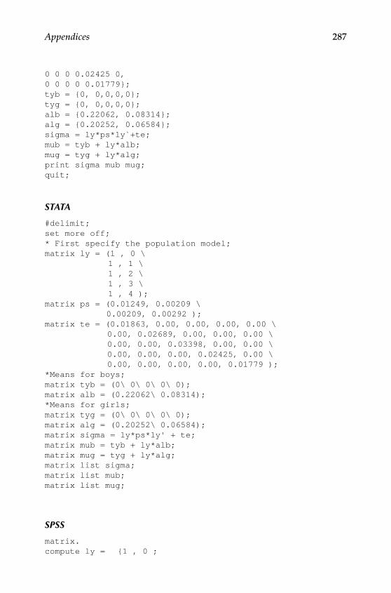
Appendices 287
0 0 0 0.02425 0,0 0 0 0 0.01779};tyb = {0, 0,0,0,0};tyg = {0, 0,0,0,0};alb = {0.22062, 0.08314};alg = {0.20252, 0.06584};sigma = ly*ps*ly`+te;mub = tyb + ly*alb;mug = tyg + ly*alg;print sigma mub mug;quit;
STATA
#delimit;set more off;* First specify the population model;matrix ly = (1 , 0 \ 1 , 1 \ 1 , 2 \ 1 , 3 \ 1 , 4 );matrix ps = (0.01249, 0.00209 \ 0.00209, 0.00292 );matrix te = (0.01863, 0.00, 0.00, 0.00, 0.00 \ 0.00, 0.02689, 0.00, 0.00, 0.00 \ 0.00, 0.00, 0.03398, 0.00, 0.00 \ 0.00, 0.00, 0.00, 0.02425, 0.00 \ 0.00, 0.00, 0.00, 0.00, 0.01779 );*Means for boys;matrix tyb = (0\ 0\ 0\ 0\ 0);matrix alb = (0.22062\ 0.08314);*Means for girls;matrix tyg = (0\ 0\ 0\ 0\ 0);matrix alg = (0.20252\ 0.06584);matrix sigma = ly*ps*ly' + te;matrix mub = tyb + ly*alb;matrix mug = tyg + ly*alg;matrix list sigma;matrix list mub;matrix list mug;
SPSS
matrix.compute ly = {1 , 0 ;
Y100315.indb 287 7/15/09 3:00:22 PM
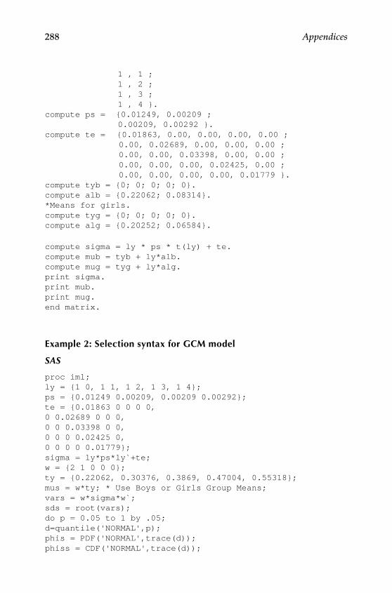
288 Appendices
1 , 1 ; 1 , 2 ; 1 , 3 ; 1 , 4 }.compute ps = {0.01249, 0.00209 ; 0.00209, 0.00292 }.compute te = {0.01863, 0.00, 0.00, 0.00, 0.00 ; 0.00, 0.02689, 0.00, 0.00, 0.00 ; 0.00, 0.00, 0.03398, 0.00, 0.00 ; 0.00, 0.00, 0.00, 0.02425, 0.00 ; 0.00, 0.00, 0.00, 0.00, 0.01779 }.compute tyb = {0; 0; 0; 0; 0}.compute alb = {0.22062; 0.08314}.*Means for girls.compute tyg = {0; 0; 0; 0; 0}.compute alg = {0.20252; 0.06584}.
compute sigma = ly * ps * t(ly) + te.compute mub = tyb + ly*alb.compute mug = tyg + ly*alg.print sigma.print mub.print mug.end matrix.
example 2: Selection syntax for gCM model
SAS
proc iml;ly = {1 0, 1 1, 1 2, 1 3, 1 4};ps = {0.01249 0.00209, 0.00209 0.00292};te = {0.01863 0 0 0 0,0 0.02689 0 0 0,0 0 0.03398 0 0,0 0 0 0.02425 0,0 0 0 0 0.01779};sigma = ly*ps*ly`+te;w = {2 1 0 0 0};ty = {0.22062, 0.30376, 0.3869, 0.47004, 0.55318};mus = w*ty; * Use Boys or Girls Group Means;vars = w*sigma*w`;sds = root(vars);do p = 0.05 to 1 by .05;d=quantile('NORMAL',p);phis = PDF('NORMAL',trace(d));phiss = CDF('NORMAL',trace(d));
Y100315.indb 288 7/15/09 3:00:22 PM
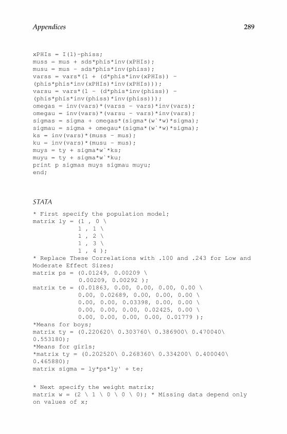
Appendices 289
xPHIs = I(1)-phiss;muss = mus + sds*phis*inv(xPHIs);musu = mus - sds*phis*inv(phiss);varss = vars*(1 + (d*phis*inv(xPHIs)) -(phis*phis*inv(xPHIs)*inv(xPHIs)));varsu = vars*(1 - (d*phis*inv(phiss)) -(phis*phis*inv(phiss)*inv(phiss)));omegas = inv(vars)*(varss - vars)*inv(vars);omegau = inv(vars)*(varsu - vars)*inv(vars);sigmas = sigma + omegas*(sigma*(w`*w)*sigma);sigmau = sigma + omegau*(sigma*(w`*w)*sigma);ks = inv(vars)*(muss - mus);ku = inv(vars)*(musu - mus);muys = ty + sigma*w`*ks;muyu = ty + sigma*w`*ku;print p sigmas muys sigmau muyu;end;
STATA
* First specify the population model;matrix ly = (1 , 0 \ 1 , 1 \ 1 , 2 \ 1 , 3 \ 1 , 4 );* Replace These Correlations with .100 and .243 for Low and Moderate Effect Sizes;matrix ps = (0.01249, 0.00209 \ 0.00209, 0.00292 );matrix te = (0.01863, 0.00, 0.00, 0.00, 0.00 \ 0.00, 0.02689, 0.00, 0.00, 0.00 \ 0.00, 0.00, 0.03398, 0.00, 0.00 \ 0.00, 0.00, 0.00, 0.02425, 0.00 \ 0.00, 0.00, 0.00, 0.00, 0.01779 );*Means for boys;matrix ty = (0.220620\ 0.303760\ 0.386900\ 0.470040\ 0.553180);*Means for girls;*matrix ty = (0.202520\ 0.268360\ 0.334200\ 0.400040\ 0.465880);matrix sigma = ly*ps*ly' + te;
* Next specify the weight matrix;matrix w = (2 \ 1 \ 0 \ 0 \ 0); * Missing data depend only on values of x;
Y100315.indb 289 7/15/09 3:00:22 PM

290 Appendices
* Mean of Selection Variable -- Selection on Observed Variables;matrix mus = w'*ty;
* Variance of Selection Variable;matrix vars = w'*sigma*w;
* Standard Deviation of Selection Variable;matrix sds = cholesky(vars);
* Mean and variance in selected subsample (greater than or equal to cutpoint);* This syntax calculates from 5% to 95% cutpoints;forvalues prob=.05(.05) 1 {;matrix z = invnorm(`prob');
* PDF(z);matrix phis = normalden(trace(z));
* CDF(z) and CDF(-z);matrix PHIs = normal(trace(z));
* 1 - CDF(z), ie CDF(-z);matrix xPHIs = I(1) - PHIs;
* Mean of Selection Variable in Selected and Unselected Portions of Sample;matrix muss = mus + sds*phis*inv(xPHIs);matrix musu = mus - sds*phis*inv(PHIs);
* Variance of Selection Variable in Selected and Unselected Portions of Sample;matrix varss = vars*(1 + (z*phis*inv(xPHIs)) -(phis*phis*inv(xPHIs)*inv(xPHIs)));matrix varsu = vars*(1 - (z*phis*inv(PHIs)) -(phis*phis*inv(PHIs)*inv(PHIs)));
* Standard Deviation of Selection Variable in Selected and Unselected Portions of Sample;matrix sdss = cholesky(varss);matrix sdsu = cholesky(varsu);
* Calculate Omega (Selected and Unselected);matrix omegas = inv(vars)*(varss - vars)*inv(vars);matrix omegau = inv(vars)*(varsu - vars)*inv(vars);
Y100315.indb 290 7/15/09 3:00:22 PM

Appendices 291
* Calculate Simga (Selected and Unselected);matrix sigmas = sigma + omegas*(sigma*(w*w')*sigma);matrix sigmau = sigma + omegau*(sigma*(w*w')*sigma);
* Calculate Kappa (Selected and Unselected);matrix ks = inv(vars)*(muss - mus);matrix ku = inv(vars)*(musu - mus);
* Calculate Muy (Selected and Unselected);matrix muys =ty + sigma*w*ks;matrix muyu = ty + sigma*w*ku;
matrix list PHIs;matrix list sigmas;matrix list muys;matrix list sigmau;matrix list muyu;matrix list sigma;};
log close;
SPSS
Input program.Loop I = 0.05 to 1 by (.05). End case.End Loop.End File.End Input Program.Execute.
COMPUTE d = IDF.NORMAL(I, 0,1).COMPUTE phis = PDF.NORMAL(d ,0,1).Compute phiss = CDFNORM(d).execute.
matrix.
Get D/variables = d.
Get PHIS/variables = phis.
Get PHISS/variables = phiss.
Y100315.indb 291 7/15/09 3:00:22 PM

292 Appendices
compute ly = {1,0;1,1;1,2;1,3;1,4}.
compute ps = {0.01249, 0.00209;0.00209, 0.00292}.
compute te ={0.01863, 0.00, 0.00, 0.00, 0.00 ; 0.00, 0.02689, 0.00, 0.00, 0.00 ; 0.00, 0.00, 0.03398, 0.00, 0.00 ; 0.00, 0.00, 0.00, 0.02425, 0.00 ; 0.00, 0.00, 0.00, 0.00, 0.01779 }.
compute ty ={0.220620; 0.303760; 0.386900; 0.470040; 0.553180}.
compute w = {2, 1, 0, 0, 0}.
compute sigma = ly * ps * t(ly) + te.
* Mean of Selection variable -- Selection on Observed Variables.compute mus = w*ty.
* Variance of Selection Variable.compute vars = w*sigma*t(w).
* Standard Deviation of Selection Variable.compute sds = chol(vars).
loop i=1 to 19.compute missamt = 5*i.compute xPHIs = ident(1) - phiss.
compute muss = mus + sds*phis(i)*inv(xphis(i)).compute musu = mus - sds*phis(i)*inv(phiss(i)).
compute varss = vars *(1 + (d(i)*phis(i)*inv(xPHIs(i))) - (phis(i)*phis(i)*inv(xPHIs(i))*inv(xPHIs(i)))).compute varsu = vars *(1 - (d(i)*phis(i)*inv(phiss(i))) -
(phis(i)*phis(i)*inv(phiss(i))*inv(phiss(i)))).compute omegas = inv(vars)*(varss - vars)*inv(vars).compute omegau = inv(vars)*(varsu - vars)*inv(vars).
compute sigmas = sigma + omegas* (sigma*(t(w)*w)*sigma).compute sigmau = sigma + omegau* (sigma*(t(w)*w)*sigma).
Y100315.indb 292 7/15/09 3:00:22 PM

Appendices 293
compute ks = inv(vars)*(muss - mus).compute ku = inv(vars)*(musu - mus).
compute muys = ty + sigma*t(w)*ks.compute muyu = ty + sigma*t(w)*ku.
print missamt.print sigmas.print muys.print sigmau.print muyu.end loop.end matrix.execute.
gCM – Saturated
LISREL
! Saturated Model! GCM Boys Complete Datada ni=5 no=500 ng=4lat1 t2 t3 t4 t5cm0.031120.01458 0.046480.01667 0.02460 0.066510.01876 0.02961 0.04046 0.075560.02085 0.03462 0.04839 0.06216 0.09372me0.22062 0.30376 0.38690 0.47004 0.55318mo ny=5 ne=2 ly=fu,fi ps=sy,fr te=sy,fi ty=fi al=frva 1.0 ly(1,1) ly(2,1) ly(3,1) ly(4,1) ly(5,1)va 0.0 ly(1,2)va 1.0 ly(2,2)va 2.0 ly(3,2)va 3.0 ly(4,2)va 4.0 ly(5,2)fr te(1,1) te(2,2) te(3,3) te(4,4) te(5,5)ou nd=5! GCM Boys Missing Datada ni=5 no=500 ng=4lat1 t2 t3 t4 t5cm0.031120.01458 0.046480.0000 0.0000 1.00000.0000 0.0000 0.0000 1.0000
Y100315.indb 293 7/15/09 3:00:22 PM
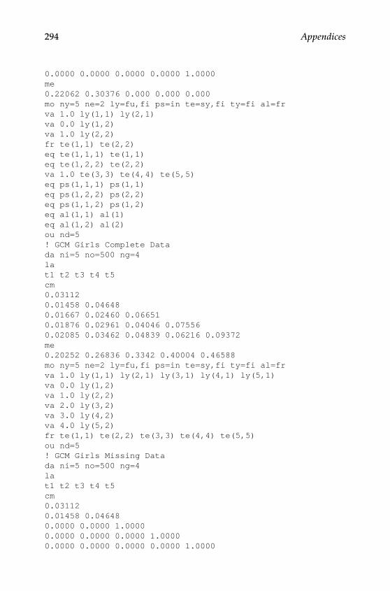
294 Appendices
0.0000 0.0000 0.0000 0.0000 1.0000me0.22062 0.30376 0.000 0.000 0.000mo ny=5 ne=2 ly=fu,fi ps=in te=sy,fi ty=fi al=frva 1.0 ly(1,1) ly(2,1)va 0.0 ly(1,2)va 1.0 ly(2,2)fr te(1,1) te(2,2)eq te(1,1,1) te(1,1)eq te(1,2,2) te(2,2)va 1.0 te(3,3) te(4,4) te(5,5)eq ps(1,1,1) ps(1,1)eq ps(1,2,2) ps(2,2)eq ps(1,1,2) ps(1,2)eq al(1,1) al(1)eq al(1,2) al(2)ou nd=5! GCM Girls Complete Datada ni=5 no=500 ng=4lat1 t2 t3 t4 t5cm0.031120.01458 0.046480.01667 0.02460 0.066510.01876 0.02961 0.04046 0.075560.02085 0.03462 0.04839 0.06216 0.09372me0.20252 0.26836 0.3342 0.40004 0.46588mo ny=5 ne=2 ly=fu,fi ps=in te=sy,fi ty=fi al=frva 1.0 ly(1,1) ly(2,1) ly(3,1) ly(4,1) ly(5,1)va 0.0 ly(1,2)va 1.0 ly(2,2)va 2.0 ly(3,2)va 3.0 ly(4,2)va 4.0 ly(5,2)fr te(1,1) te(2,2) te(3,3) te(4,4) te(5,5)ou nd=5! GCM Girls Missing Datada ni=5 no=500 ng=4lat1 t2 t3 t4 t5cm0.031120.01458 0.046480.0000 0.0000 1.00000.0000 0.0000 0.0000 1.00000.0000 0.0000 0.0000 0.0000 1.0000
Y100315.indb 294 7/15/09 3:00:22 PM

Appendices 295
me0.20252 0.26836 0.000 0.000 0.000mo ny=5 ne=2 ly=fu,fi ps=in te=sy,fi ty=fi al=frva 1.0 ly(1,1) ly(2,1)va 0.0 ly(1,2)va 1.0 ly(2,2)fr te(1,1) te(2,2)eq te(3,1,1) te(1,1)eq te(3,2,2) te(2,2)va 1.0 te(3,3) te(4,4) te(5,5)eq ps(3,1,1) ps(1,1)eq ps(3,2,2) ps(2,2)eq ps(3,1,2) ps(1,2)eq al(3,1) al(1)eq al(3,2) al(2)ou nd=5
MPLUS
TITLE: Chapter 7 - Saturated;DATA: FILE is GCM_Saturated.dat; TYPE IS MEANS COVARIANCE; NGROUPS=4; NOBSERVATION = 500 500 500 500;VARIABLE: NAMES are t1 t2 t3 t4 t5;ANALYSIS: TYPE=MEANSTRUCTURE;MODEL: !Intercept and Slope Loadings; i BY t1-t5@1; s BY [email protected] [email protected] [email protected] [email protected] [email protected]; !Means for observed variables fixed to 0; [t1-t5@0]; !Error Variance are estimated; t1(1); t2(2); t3-t5; !Covariance and variance of intercept and slope are estimated; i with s(3); i(4); s(5);
Model G1: !Means for intercept and slope free and equated to Group 2; [i](6); [s](7);Model G2: !Intercept and Slope Loadings for Group 2; i BY [email protected] t3-t5@0; s BY t1@0 [email protected] t3-t5@0;
Y100315.indb 295 7/15/09 3:00:22 PM

296 Appendices
!Error variance of t1 and t2 equated to Group 1; t1(1); t2(2); !Error variance of t3 through t5 fixed at 1; t3-t5@1; !Covariance and variance of intercept and slope equated to Group 1; i with s(3); i(4); s(5); !Means for intercept and slope equated to Group 1; [i](6); [s](7); !Means for observed variables fixed to 0; [t1-t5@0];
Model G3: !Intercept and Slope Loading for Group 3; i BY t1-t5@1; s BY t1@0 t2@1 t3@2 t4@3 t5@4; !Error variances are estimated; t1(8); t2(9); t3-t5; !Covaraince and variance of intercept and slope are estimated; i with s(3); i(4); s(5); !Means for intercept and slope free and equated to Group 2; [i](13); [s](14); !Means for observed variables fixed to 0; [t1-t5@0];
Model G4: i BY [email protected] [email protected] t3@0 t4@0 t5@0; s BY t1@0 [email protected] t3-t5@0; !Error Variance of t1 and t2 equated to Group 2; t1(8); t2(9); !Error variance of t3 through t5 fixed at 1; t3-t5@1;
!Covariance and variance of intercept and slope equated to Group 1; i with s(3); i(4); s(5);
Y100315.indb 296 7/15/09 3:00:22 PM

Appendices 297
!Means for intercept and slope equated to Group 1; [i](13); [s](14); !Means for observed variables fixed to 0; [t1-t5@0];OUTPUT: !For Fmin, see the last value from the function column of TECH5; RESIDUAL TECH1 TECH5;
AMOS
#Region "Header"Imports SystemImports System.DiagnosticsImports Microsoft.VisualBasicImports AmosEngineLibImports AmosGraphicsImports AmosEngineLib.AmosEngine.TMatrixIDImports PBayes#End RegionModule MainModule Sub Main() Dim Sem As New AmosEngine Try Sem.TextOutput() Sem.ModelMeansAndIntercepts() Sem.BeginGroup("C:\Documents and Settings\Tina Salva\My Documents\LEA Book\Application 3\GCM_Saturated_BoysComplete.xls", "Sheet1") Sem.GroupName("Boys Complete") 'Factor Loadings Sem.AStructure("t1 = (0) + (1) LEVEL + (0) SLOPE + (1) E1") Sem.AStructure("t2 = (0) + (1) LEVEL + (1) SLOPE + (1) E2") Sem.AStructure("t3 = (0) + (1) LEVEL + (2) SLOPE + (1) E3") Sem.AStructure("t4 = (0) + (1) LEVEL + (3) SLOPE + (1) E4") Sem.AStructure("t5 = (0) + (1) LEVEL + (4) SLOPE + (1) E5") 'Factor Variances Sem.Var("LEVEL", "var_level_boys") Sem.Var("SLOPE", "var_slope_boys") Sem.Cov("LEVEL", "SLOPE", "lscov_boys") 'Mean 'Intercept
Y100315.indb 297 7/15/09 3:00:22 PM

298 Appendices
Sem.Mean ("LEVEL", "mean_level_boys") Sem.Mean ("SLOPE", "mean_slope_boys") 'Error Variances Sem.Var("E1", "e1_boys") Sem.Var("E2", "e2_boys") Sem.Var("E3", "e3_boys") Sem.Var("E4", "e4_boys") Sem.Var("E5", "e5_boys") Sem.BeginGroup("C:\Documents and Settings\Tina Salva\My Documents\LEA Book\Application 3\GCM_Saturated_BoysMissing.xls", "Sheet1") Sem.GroupName("Boys Missing") 'Factor Loadings Sem.AStructure("t1 = (0) + (1) LEVEL + (0) SLOPE + (1) E1") Sem.AStructure("t2 = (0) + (1) LEVEL + (1) SLOPE + (1) E2") Sem.AStructure("t3 = (0) + (0) LEVEL + (0) SLOPE + (1) E3") Sem.AStructure("t4 = (0) + (0) LEVEL + (0) SLOPE + (1) E4") Sem.AStructure("t5 = (0) + (0) LEVEL + (0) SLOPE + (1) E5") 'Factor Variances Sem.Var("LEVEL", "var_level_boys") Sem.Var("SLOPE", "var_slope_boys") Sem.Cov("LEVEL", "SLOPE", "lscov_boys") 'Mean 'Intercept Sem.Mean ("LEVEL", "mean_level_boys") Sem.Mean ("SLOPE", "mean_slope_boys") 'Error Variances Sem.Var("E1", "e1_boys") Sem.Var("E2", "e2_boys") Sem.Var("E3", "1") Sem.Var("E4", "1") Sem.Var("E5", "1") Sem.BeginGroup("C:\Documents and Settings\Tina Salva\My Documents\LEA Book\Application 3\GCM_Saturated_GirlsComplete.xls", "Sheet1") Sem.GroupName("Girls Complete") 'Factor Loadings
Y100315.indb 298 7/15/09 3:00:22 PM

Appendices 299
Sem.AStructure("t1 = (0) + (1) LEVEL + (0) SLOPE + (1) E1") Sem.AStructure("t2 = (0) + (1) LEVEL + (1) SLOPE + (1) E2") Sem.AStructure("t3 = (0) + (1) LEVEL + (2) SLOPE + (1) E3") Sem.AStructure("t4 = (0) + (1) LEVEL + (3) SLOPE + (1) E4") Sem.AStructure("t5 = (0) + (1) LEVEL + (4) SLOPE + (1) E5") 'Factor Variances Sem.Var("LEVEL", "var_level_boys") Sem.Var("SLOPE", "var_slope_boys") Sem.Cov("LEVEL", "SLOPE", "lscov_boys") 'Mean 'Intercept Sem.Mean ("LEVEL", "mean_level_girls") Sem.Mean ("SLOPE", "mean_slope_girls") 'Error Variances Sem.Var("E1", "e1_girls") Sem.Var("E2", "e2_girls") Sem.Var("E3", "e3_girls") Sem.Var("E4", "e4_girls") Sem.Var("E5", "e5_girls") Sem.BeginGroup("C:\Documents and Settings\Tina Salva\My Documents\LEA Book\Application 3\GCM_Saturated_GirlsMissing.xls", "Sheet1") Sem.GroupName("Girls Missing") 'Factor Loadings Sem.AStructure("t1 = (0) + (1) LEVEL + (0) SLOPE + (1) E1") Sem.AStructure("t2 = (0) + (1) LEVEL + (1) SLOPE + (1) E2") Sem.AStructure("t3 = (0) + (0) LEVEL + (0) SLOPE + (1) E3") Sem.AStructure("t4 = (0) + (0) LEVEL + (0) SLOPE + (1) E4") Sem.AStructure("t5 = (0) + (0) LEVEL + (0) SLOPE + (1) E5") 'Factor Variances Sem.Var("LEVEL", "var_level_boys") Sem.Var("SLOPE", "var_slope_boys") Sem.Cov("LEVEL", "SLOPE", "lscov_boys") 'Mean 'Intercept
Y100315.indb 299 7/15/09 3:00:22 PM

300 Appendices
Sem.Mean ("LEVEL", "mean_level_girls") Sem.Mean ("SLOPE", "mean_slope_girls") 'Error Variances Sem.Var("E1", "e1_girls") Sem.Var("E2", "e2_girls") Sem.Var("E3", "1") Sem.Var("E4", "1") Sem.Var("E5", "1") Sem.FitAllModels Finally Sem.Dispose() End Try End SubEnd Module
Power for a given NCP, DF, alPHa
SAS
data power; do n = 50 to 1000 by 50; g = 2; alpha = 0.05; df = 1; fmin = 0.011093 ncp = (n-g)*fmin; chicrit = quantile('chisquare',1-alpha, 1); power = 1- PROBCHI(chicrit,df,ncp);*power = 1-CDF('chisquare', chicrit, df, ncp) ; output; end;proc print data=power; var n alpha df ncp power;run;
STATA
#delimit;set more off;set obs 20;gen FMin = 0.011093;gen n = 50*_n;gen ncp = (n-1)*FMin;gen df = 1;gen alpha = 0.05;
Y100315.indb 300 7/15/09 3:00:22 PM

Appendices 301
gen chicrit = invchi2tail(df, alpha);gen power = 1- nchi2(df,ncp,chicrit);list n ncp power, noobs clean table;
SPSS
DATA LIST FREE / obs.BEGIN DATA.1 2 3 4 5 6 7 8 9 10 11 12 13 14 15 16 17 18 19 20END DATA.Compute FMin = 0.011093.compute n = 50*obs.Compute ncp = (n-1)*FMin.compute df = 1.compute alpha = 0.05.Compute chicrit = IDF.CHISQ(1-alpha,df) .Compute power = 1-NCDF.CHISQ(chicrit, df, ncp) .execute.list n ncp power .
NCP & Sample Size for a given DF, alpha and Power
SAS
data ncp; alpha = 0.05; power = 0.80; fmin = 0.011093 do df = 1 to 10; chicrit = quantile('chisquare',1-alpha, df); ncp = CINV(power, df, chicrit); n0=ncp/fmin; output; end;proc print data=ncp; var df chicrit ncp n0;run;
STATA
#delimit;set more off;set obs 10;generate df = _n;generate alpha = 0.05;generate power =0.80;gen chicrit = invchi2tail(df, alpha);gen ncp = invnchi2(df,chicrit,power);
Y100315.indb 301 7/15/09 3:00:23 PM
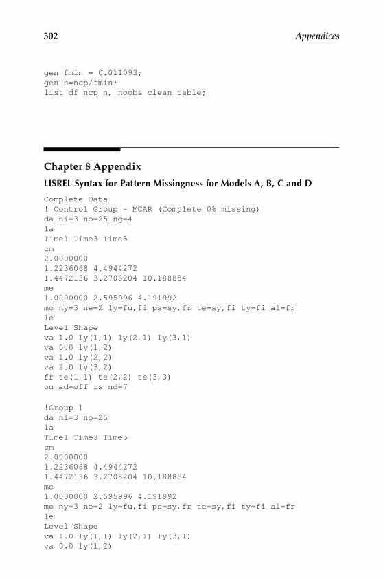
302 Appendices
gen fmin = 0.011093;gen n=ncp/fmin;list df ncp n, noobs clean table;
Chapter 8 Appendix
liSrel Syntax for Pattern Missingness for Models a, b, C and D
Complete Data! Control Group - MCAR (Complete 0% missing)da ni=3 no=25 ng=4laTime1 Time3 Time5cm2.00000001.2236068 4.49442721.4472136 3.2708204 10.188854me1.0000000 2.595996 4.191992mo ny=3 ne=2 ly=fu,fi ps=sy,fr te=sy,fi ty=fi al=frleLevel Shapeva 1.0 ly(1,1) ly(2,1) ly(3,1)va 0.0 ly(1,2)va 1.0 ly(2,2)va 2.0 ly(3,2)fr te(1,1) te(2,2) te(3,3)ou ad=off rs nd=7
!Group 1da ni=3 no=25laTime1 Time3 Time5cm2.00000001.2236068 4.49442721.4472136 3.2708204 10.188854me1.0000000 2.595996 4.191992mo ny=3 ne=2 ly=fu,fi ps=sy,fr te=sy,fi ty=fi al=frleLevel Shapeva 1.0 ly(1,1) ly(2,1) ly(3,1)va 0.0 ly(1,2)
Y100315.indb 302 7/15/09 3:00:23 PM
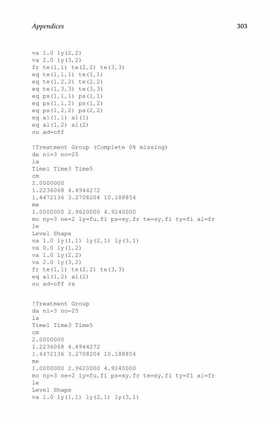
Appendices 303
va 1.0 ly(2,2)va 2.0 ly(3,2)fr te(1,1) te(2,2) te(3,3)eq te(1,1,1) te(1,1)eq te(1,2,2) te(2,2)eq te(1,3,3) te(3,3)eq ps(1,1,1) ps(1,1)eq ps(1,1,2) ps(1,2)eq ps(1,2,2) ps(2,2)eq al(1,1) al(1)eq al(1,2) al(2)ou ad=off
!Treatment Group (Complete 0% missing)da ni=3 no=25laTime1 Time3 Time5cm2.00000001.2236068 4.49442721.4472136 3.2708204 10.188854me1.0000000 2.9620000 4.9240000mo ny=3 ne=2 ly=fu,fi ps=sy,fr te=sy,fi ty=fi al=frleLevel Shapeva 1.0 ly(1,1) ly(2,1) ly(3,1)va 0.0 ly(1,2)va 1.0 ly(2,2)va 2.0 ly(3,2)fr te(1,1) te(2,2) te(3,3)eq al(1,2) al(2)ou ad=off rs
!Treatment Groupda ni=3 no=25laTime1 Time3 Time5cm2.00000001.2236068 4.49442721.4472136 3.2708204 10.188854me1.0000000 2.9620000 4.9240000mo ny=3 ne=2 ly=fu,fi ps=sy,fr te=sy,fi ty=fi al=frleLevel Shapeva 1.0 ly(1,1) ly(2,1) ly(3,1)
Y100315.indb 303 7/15/09 3:00:23 PM
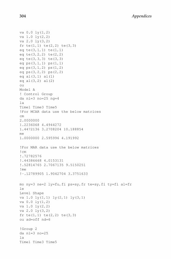
304 Appendices
va 0.0 ly(1,2)va 1.0 ly(2,2)va 2.0 ly(3,2)fr te(1,1) te(2,2) te(3,3)eq te(3,1,1) te(1,1)eq te(3,2,2) te(2,2)eq te(3,3,3) te(3,3)eq ps(3,1,1) ps(1,1)eq ps(3,1,2) ps(1,2)eq ps(3,2,2) ps(2,2)eq al(3,1) al(1)eq al(3,2) al(2)ouModel A! Control Groupda ni=3 no=25 ng=4laTime1 Time3 Time5!For MCAR data use the below matricescm2.00000001.2236068 4.49442721.4472136 3.2708204 10.188854me1.0000000 2.595996 4.191992
!For MAR data use the below matrices!cm!.72782576!.44386668 4.0153131!.52814765 2.7067135 9.5150251!me!-.12789905 1.9042704 3.3751633
mo ny=3 ne=2 ly=fu,fi ps=sy,fr te=sy,fi ty=fi al=frleLevel Shapeva 1.0 ly(1,1) ly(2,1) ly(3,1)va 0.0 ly(1,2)va 1.0 ly(2,2)va 2.0 ly(3,2)fr te(1,1) te(2,2) te(3,3)ou ad=off nd=6
!Group 2da ni=3 no=25laTime1 Time3 Time5
Y100315.indb 304 7/15/09 3:00:23 PM
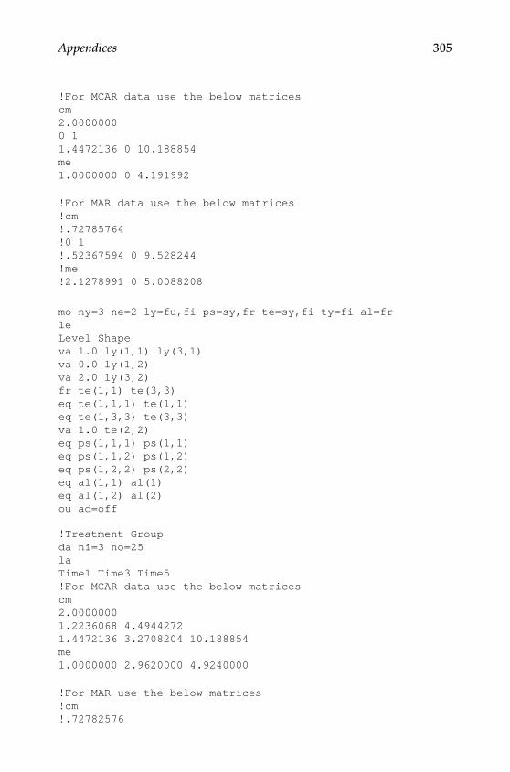
Appendices 305
!For MCAR data use the below matricescm2.00000000 11.4472136 0 10.188854me1.0000000 0 4.191992
!For MAR data use the below matrices!cm!.72785764!0 1!.52367594 0 9.528244!me!2.1278991 0 5.0088208
mo ny=3 ne=2 ly=fu,fi ps=sy,fr te=sy,fi ty=fi al=frleLevel Shapeva 1.0 ly(1,1) ly(3,1)va 0.0 ly(1,2)va 2.0 ly(3,2)fr te(1,1) te(3,3)eq te(1,1,1) te(1,1)eq te(1,3,3) te(3,3)va 1.0 te(2,2)eq ps(1,1,1) ps(1,1)eq ps(1,1,2) ps(1,2)eq ps(1,2,2) ps(2,2)eq al(1,1) al(1)eq al(1,2) al(2)ou ad=off
!Treatment Groupda ni=3 no=25laTime1 Time3 Time5!For MCAR data use the below matricescm2.00000001.2236068 4.49442721.4472136 3.2708204 10.188854me1.0000000 2.9620000 4.9240000
!For MAR use the below matrices!cm!.72782576
Y100315.indb 305 7/15/09 3:00:23 PM
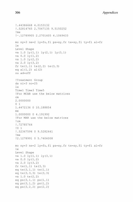
306 Appendices
!.44386668 4.0153132!.52814765 2.7067135 9.5150252!me!-.12789905 2.2701605 4.1069433
mo ny=3 ne=2 ly=fu,fi ps=sy,fr te=sy,fi ty=fi al=frleLevel Shapeva 1.0 ly(1,1) ly(2,1) ly(3,1)va 0.0 ly(1,2)va 1.0 ly(2,2)va 2.0 ly(3,2)fr te(1,1) te(2,2) te(3,3)eq al(1,2) al(2)ou ad=off
!Treatment Groupda ni=3 no=25laTime1 Time3 Time5!For MCAR use the below matricescm2.00000000 11.4472136 0 10.188854me1.0000000 0 4.191992!For MAR use the below matrices!cm!.72785764!0 1!.52367594 0 9.5282441!me!2.1278991 0 5.7406008
mo ny=3 ne=2 ly=fu,fi ps=sy,fr te=sy,fi ty=fi al=frleLevel Shapeva 1.0 ly(1,1) ly(3,1)va 0.0 ly(1,2)va 2.0 ly(3,2)fr te(1,1) te(3,3)eq te(3,1,1) te(1,1)eq te(3,3,3) te(3,3)va 1.0 te(2,2)eq ps(3,1,1) ps(1,1)eq ps(3,1,2) ps(1,2)eq ps(3,2,2) ps(2,2)
Y100315.indb 306 7/15/09 3:00:23 PM

Appendices 307
eq al(3,1) al(1)eq al(3,2) al(2)ou
Model A - Saturated Model! Control Groupda ni=3 no=25 ng=4laTime1 Time3 Time5cm.72782576.44386668 4.0153131.52814765 2.7067135 9.5150251me-.12789905 1.9042704 3.3751633mo ny=3 ne=3 ly=fu,fi ps=sy,fr te=sy,fi ty=frva 1.0 ly(1,1)va 1.0 ly(2,2)va 1.0 ly(3,3)ou ad=off nd=6
!Group 2da ni=3 no=25laTime1 Time3 Time5cm.727857640 1.52367594 0 9.528244me2.1278991 0 5.0088208mo ny=3 ne=3 ly=fu,fi ps=in te=sy,fi ty=frva 1.0 ly(1,1)va 1.0 ly(3,3)fr ty(1) ty(3)eq ty(1,1) ty(1)eq ty(1,3) ty(3)fi ty(2)va 1.0 te(2,2)ou ad=off
!Treatment Groupda ni=3 no=25laTime1 Time3 Time5cm.72782576.44386668 4.0153132
Y100315.indb 307 7/15/09 3:00:23 PM

308 Appendices
.52814765 2.7067135 9.5150252me-.12789905 2.2701605 4.1069433mo ny=3 ne=3 ly=fu,fi ps=sy,fr te=sy,fi ty=frva 1.0 ly(1,1)va 1.0 ly(2,2)va 1.0 ly(3,3)ou ad=off
!Treatment Groupda ni=3 no=25laTime1 Time3 Time5cm.727857640 1.52367594 0 9.5282441me2.1278991 0 5.7406008mo ny=3 ne=3 ly=fu,fi ps=sy,fr te=sy,fi ty=frva 1.0 ly(1,1)va 1.0 ly(3,3)eq ps(3,1,1) ps(1,1)eq ps(3,2,1) ps(2,1)eq ps(3,2,2) ps(2,2)eq ps(3,3,1) ps(3,1)eq ps(3,3,2) ps(3,2)eq ps(3,3,3) ps(3,3)fr ty(1) ty(3)eq ty(3,1) ty(1)eq ty(3,3) ty(3)fi ty(2)va 1.0 te(2,2)ou ad=off
Model B!Study 1 Control Group - MCAR (Complete 0% missing)da ni=3 no=25 ng=4laTime1 Time3 Time5!For MCAR use the below matricescm2.00000001.2236068 4.49442721.4472136 3.2708204 10.188854me1.0000000 2.595996 4.191992
!For MAR use the below matrices
Y100315.indb 308 7/15/09 3:00:23 PM

Appendices 309
cm.72782576.44386668 4.0153131.52814765 2.7067135 9.5150251me-.12789905 1.9042704 3.3751633
mo ny=3 ne=2 ly=fu,fi ps=sy,fr te=sy,fi ty=fi al=frleLevel Shapeva 1.0 ly(1,1) ly(2,1) ly(3,1)va 0.0 ly(1,2)va 1.0 ly(2,2)va 2.0 ly(3,2)fr te(1,1) te(2,2) te(3,3)ou ad=off nd=5
!Group 2 Miss Wave 3da ni=3 no=25laTime1 Time3 Time5!For MCAR use the below matricescm2.00000001.2236068 4.49442720 0 1me1.0000000 2.595996 0!For MAR use the below matrices!cm!.72785764!.44295123 4.0165637!0 0 1!me!2.1278991 3.2877216 0
mo ny=3 ne=2 ly=fu,fi ps=sy,fr te=sy,fi ty=fi al=frleLevel Shapeva 1.0 ly(1,1) ly(2,1)va 0.0 ly(1,2)va 1.0 ly(2,2)fr te(1,1) te(2,2)eq te(1,1,1) te(1,1)eq te(1,2,2) te(2,2)va 1.0 te(3,3)eq ps(1,1,1) ps(1,1)eq ps(1,1,2) ps(1,2)eq ps(1,2,2) ps(2,2)
Y100315.indb 309 7/15/09 3:00:23 PM
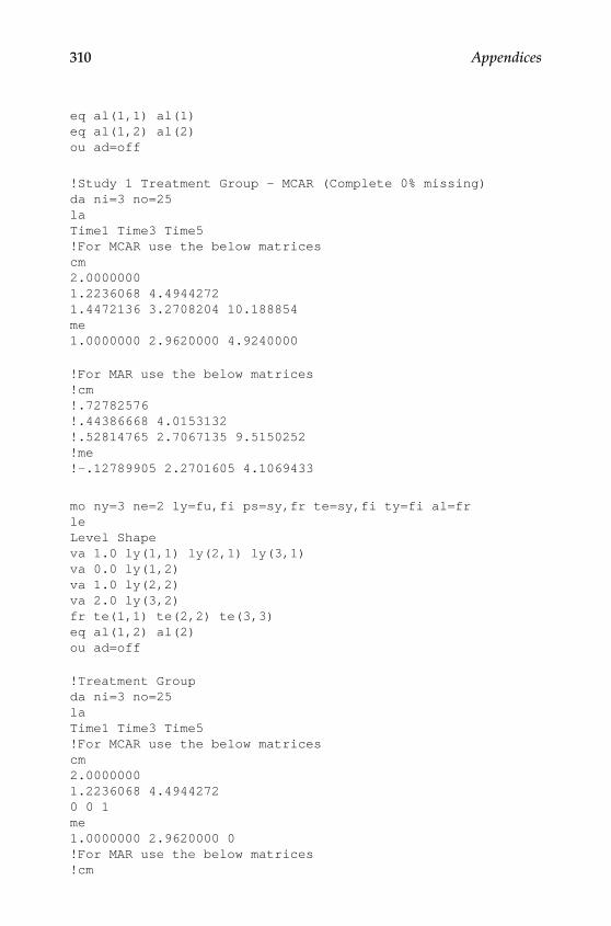
310 Appendices
eq al(1,1) al(1)eq al(1,2) al(2)ou ad=off
!Study 1 Treatment Group - MCAR (Complete 0% missing)da ni=3 no=25laTime1 Time3 Time5!For MCAR use the below matricescm2.00000001.2236068 4.49442721.4472136 3.2708204 10.188854me1.0000000 2.9620000 4.9240000
!For MAR use the below matrices!cm!.72782576!.44386668 4.0153132!.52814765 2.7067135 9.5150252!me!-.12789905 2.2701605 4.1069433
mo ny=3 ne=2 ly=fu,fi ps=sy,fr te=sy,fi ty=fi al=frleLevel Shapeva 1.0 ly(1,1) ly(2,1) ly(3,1)va 0.0 ly(1,2)va 1.0 ly(2,2)va 2.0 ly(3,2)fr te(1,1) te(2,2) te(3,3)eq al(1,2) al(2)ou ad=off
!Treatment Groupda ni=3 no=25laTime1 Time3 Time5!For MCAR use the below matricescm2.00000001.2236068 4.49442720 0 1me1.0000000 2.9620000 0!For MAR use the below matrices!cm
Y100315.indb 310 7/15/09 3:00:23 PM
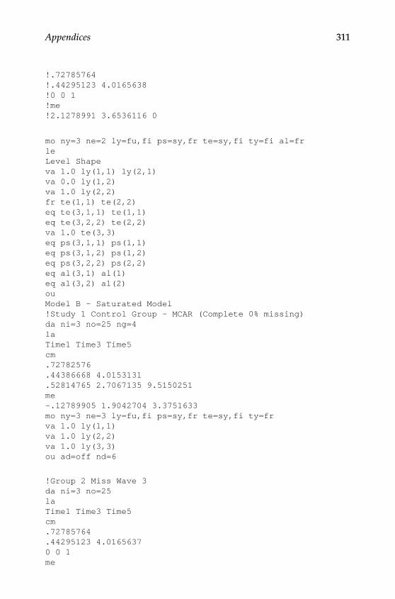
Appendices 311
!.72785764!.44295123 4.0165638!0 0 1!me!2.1278991 3.6536116 0
mo ny=3 ne=2 ly=fu,fi ps=sy,fr te=sy,fi ty=fi al=frleLevel Shapeva 1.0 ly(1,1) ly(2,1)va 0.0 ly(1,2)va 1.0 ly(2,2)fr te(1,1) te(2,2)eq te(3,1,1) te(1,1)eq te(3,2,2) te(2,2)va 1.0 te(3,3)eq ps(3,1,1) ps(1,1)eq ps(3,1,2) ps(1,2)eq ps(3,2,2) ps(2,2)eq al(3,1) al(1)eq al(3,2) al(2)ouModel B - Saturated Model!Study 1 Control Group - MCAR (Complete 0% missing)da ni=3 no=25 ng=4laTime1 Time3 Time5cm.72782576.44386668 4.0153131.52814765 2.7067135 9.5150251me-.12789905 1.9042704 3.3751633mo ny=3 ne=3 ly=fu,fi ps=sy,fr te=sy,fi ty=frva 1.0 ly(1,1)va 1.0 ly(2,2)va 1.0 ly(3,3)ou ad=off nd=6
!Group 2 Miss Wave 3da ni=3 no=25laTime1 Time3 Time5cm.72785764.44295123 4.01656370 0 1me
Y100315.indb 311 7/15/09 3:00:23 PM
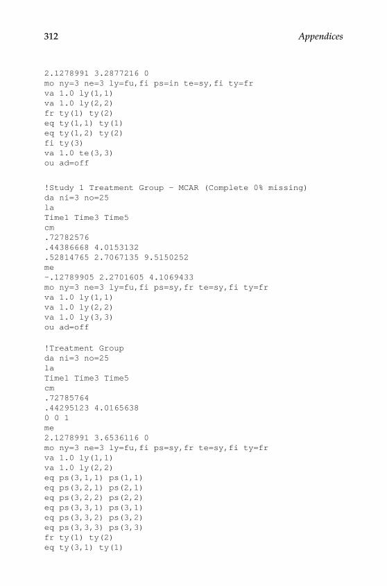
312 Appendices
2.1278991 3.2877216 0mo ny=3 ne=3 ly=fu,fi ps=in te=sy,fi ty=frva 1.0 ly(1,1)va 1.0 ly(2,2)fr ty(1) ty(2)eq ty(1,1) ty(1)eq ty(1,2) ty(2)fi ty(3)va 1.0 te(3,3)ou ad=off
!Study 1 Treatment Group - MCAR (Complete 0% missing)da ni=3 no=25laTime1 Time3 Time5cm.72782576.44386668 4.0153132.52814765 2.7067135 9.5150252me-.12789905 2.2701605 4.1069433mo ny=3 ne=3 ly=fu,fi ps=sy,fr te=sy,fi ty=frva 1.0 ly(1,1)va 1.0 ly(2,2)va 1.0 ly(3,3)ou ad=off
!Treatment Groupda ni=3 no=25laTime1 Time3 Time5cm.72785764.44295123 4.01656380 0 1me2.1278991 3.6536116 0mo ny=3 ne=3 ly=fu,fi ps=sy,fr te=sy,fi ty=frva 1.0 ly(1,1)va 1.0 ly(2,2)eq ps(3,1,1) ps(1,1)eq ps(3,2,1) ps(2,1)eq ps(3,2,2) ps(2,2)eq ps(3,3,1) ps(3,1)eq ps(3,3,2) ps(3,2)eq ps(3,3,3) ps(3,3)fr ty(1) ty(2)eq ty(3,1) ty(1)
Y100315.indb 312 7/15/09 3:00:23 PM

Appendices 313
eq ty(3,2) ty(2)fi ty(3)va 1.0 te(3,3)ou ad=off
Model C!Study 1 Control Group - MCAR (Complete 0% missing)da ni=3 no=50 ng=6laTime1 Time3 Time5!For MCAR data use the below matricescm2.00000001.2236068 4.49442721.4472136 3.2708204 10.188854me1.0000000 2.595996 4.191992
!For MAR use the below matrices!cm!.72782576!.44386668 4.0153131!.52814765 2.7067135 9.5150251!me!.12789905 1.9042704 3.3751633
mo ny=3 ne=2 ly=fu,fi ps=sy,fr te=sy,fi ty=fi al=frleLevel Shapeva 1.0 ly(1,1) ly(2,1) ly(3,1)va 0.0 ly(1,2)va 1.0 ly(2,2)va 2.0 ly(3,2)fr te(1,1) te(2,2) te(3,3)ou ad=off nd=5
!Group 2da ni=3 no=25laTime1 Time3 Time5!For MCAR use the below matricescm2.00000000 11.4472136 0 10.188854me1.0000000 0 4.191992
Y100315.indb 313 7/15/09 3:00:23 PM

314 Appendices
!For MAR use the below matrices!cm!.72785764!0 1!.52367594 0 9.528244!me!2.1278991 0 5.0088208
mo ny=3 ne=2 ly=fu,fi ps=sy,fr te=sy,fi ty=fi al=frleLevel Shapeva 1.0 ly(1,1) ly(3,1)va 0.0 ly(1,2)va 2.0 ly(3,2)fr te(1,1) te(3,3)eq te(1,1,1) te(1,1)eq te(1,3,3) te(3,3)va 1.0 te(2,2)eq ps(1,1,1) ps(1,1)eq ps(1,1,2) ps(1,2)eq ps(1,2,2) ps(2,2)eq al(1,1) al(1)eq al(1,2) al(2)ou ad=off
!Group 2 Miss Wave 3da ni=3 no=25laTime1 Time3 Time5!For MCAR use the below matricescm2.00000001.2236068 4.49442720 0 1me1.0000000 2.595996 0
!For MAR use the below matrices!cm!.72785764!.44295123 4.0165637!0 0 1!me!2.1278991 3.2877216 0
mo ny=3 ne=2 ly=fu,fi ps=sy,fr te=sy,fi ty=fi al=frleLevel Shape
Y100315.indb 314 7/15/09 3:00:23 PM

Appendices 315
va 1.0 ly(1,1) ly(2,1)va 0.0 ly(1,2)va 1.0 ly(2,2)fr te(1,1) te(2,2)eq te(1,1,1) te(1,1)eq te(1,2,2) te(2,2)va 1.0 te(3,3)eq ps(1,1,1) ps(1,1)eq ps(1,1,2) ps(1,2)eq ps(1,2,2) ps(2,2)eq al(1,1) al(1)eq al(1,2) al(2)ou ad=off
!Study 1 Treatment Group - MCAR (Complete 0% missing)da ni=3 no=50laTime1 Time3 Time5!For MCAR use the below matricescm2.00000001.2236068 4.49442721.4472136 3.2708204 10.188854me1.0000000 2.9620000 4.9240000
!For MAR use the below matrices!cm!.72782576!.44386668 4.0153132!.52814765 2.7067135 9.5150252!me!-.12789905 2.2701605 4.1069433
mo ny=3 ne=2 ly=fu,fi ps=sy,fr te=sy,fi ty=fi al=frleLevel Shapeva 1.0 ly(1,1) ly(2,1) ly(3,1)va 0.0 ly(1,2)va 1.0 ly(2,2)va 2.0 ly(3,2)fr te(1,1) te(2,2) te(3,3)eq al(1,2) al(2)ou ad=off
!Treatment Groupda ni=3 no=25la
Y100315.indb 315 7/15/09 3:00:23 PM
316 Appendices
Time1 Time3 Time5!For MCAR use the below matricescm2.00000000 11.4472136 0 10.188854me1.0000000 0 4.191992
!For MAR use the below matrices!cm!.72785764!0 1!.52367594 0 9.5282441!me!2.1278991 0 5.7406008
mo ny=3 ne=2 ly=fu,fi ps=sy,fr te=sy,fi ty=fi al=frleLevel Shapeva 1.0 ly(1,1) ly(3,1)va 0.0 ly(1,2)va 2.0 ly(3,2)fr te(1,1) te(3,3)eq te(4,1,1) te(1,1)eq te(4,3,3) te(3,3)va 1.0 te(2,2)eq ps(4,1,1) ps(1,1)eq ps(4,1,2) ps(1,2)eq ps(4,2,2) ps(2,2)eq al(4,1) al(1)eq al(4,2) al(2)ou
!Group 3 Tx Miss @ W3!Treatment Groupda ni=3 no=25laTime1 Time3 Time5!For MCAR data use the below matricescm2.00000001.2236068 4.49442720 0 1me1.0000000 2.9620000 0!For MAR data use the below matrices!cm
Y100315.indb 316 7/15/09 3:00:23 PM

Appendices 317
!.72785764!.44295123 4.0165638!0 0 1!me!2.1278991 3.6536116 0
mo ny=3 ne=2 ly=fu,fi ps=sy,fr te=sy,fi ty=fi al=frleLevel Shapeva 1.0 ly(1,1) ly(2,1)va 0.0 ly(1,2)va 1.0 ly(2,2)fr te(1,1) te(2,2)eq te(4,1,1) te(1,1)eq te(4,2,2) te(2,2)va 1.0 te(3,3)eq ps(4,1,1) ps(1,1)eq ps(4,1,2) ps(1,2)eq ps(4,2,2) ps(2,2)eq al(4,1) al(1)eq al(4,2) al(2)ou
Model 3 (Saturated Model)!Study 1 Control Group - MCAR (Complete 0% missing)da ni=3 no=50 ng=6laTime1 Time3 Time5cm.72782576.44386668 4.0153131.52814765 2.7067135 9.5150251me-.12789905 1.9042704 3.3751633mo ny=3 ne=3 ly=fu,fi ps=sy,fr te=sy,fi ty=frva 1.0 ly(1,1)va 1.0 ly(2,2)va 1.0 ly(3,3)ou ad=off nd=6
!Group 2da ni=3 no=25laTime1 Time3 Time5cm.727857640 1.52367594 0 9.528244
Y100315.indb 317 7/15/09 3:00:23 PM
318 Appendices
me2.1278991 0 5.0088208mo ny=3 ne=3 ly=fu,fi ps=in te=sy,fi ty=frva 1.0 ly(1,1)va 1.0 ly(3,3)fr ty(1) ty(3)eq ty(1,1) ty(1)eq ty(1,3) ty(3)fi ty(2)va 1.0 te(2,2)ou ad=off
!Group 2 Miss Wave 3da ni=3 no=25laTime1 Time3 Time5cm.72785764.44295123 4.01656370 0 1me2.1278991 3.2877216 0mo ny=3 ne=3 ly=fu,fi ps=in te=sy,fi ty=frva 1.0 ly(1,1)va 1.0 ly(2,2)fr ty(1) ty(2)eq ty(1,1) ty(1)eq ty(1,2) ty(2)fi ty(3)va 1.0 te(3,3)ou ad=off
!Study 1 Treatment Group - MCAR (Complete 0% missing)da ni=3 no=50laTime1 Time3 Time5cm.72782576.44386668 4.0153132.52814765 2.7067135 9.5150252me-.12789905 2.2701605 4.1069433mo ny=3 ne=3 ly=fu,fi ps=sy,fr te=sy,fi ty=frva 1.0 ly(1,1)va 1.0 ly(2,2)va 1.0 ly(3,3)ou ad=off
Y100315.indb 318 7/15/09 3:00:23 PM

Appendices 319
!Treatment Groupda ni=3 no=25laTime1 Time3 Time5cm.727857640 1.52367594 0 9.5282441me2.1278991 0 5.7406008mo ny=3 ne=3 ly=fu,fi ps=sy,fr te=sy,fi ty=frva 1.0 ly(1,1)va 1.0 ly(3,3)eq ps(4,1,1) ps(1,1)eq ps(4,2,1) ps(2,1)eq ps(4,2,2) ps(2,2)eq ps(4,3,1) ps(3,1)eq ps(4,3,2) ps(3,2)eq ps(4,3,3) ps(3,3)fr ty(1) ty(3)eq ty(4,1) ty(1)eq ty(4,3) ty(3)fi ty(2)va 1.0 te(2,2)ou ad=off
!Group 3 Tx Miss @ W3!Treatment Groupda ni=3 no=25laTime1 Time3 Time5cm.72785764.44295123 4.01656380 0 1me2.1278991 3.6536116 0mo ny=3 ne=3 ly=fu,fi ps=sy,fr te=sy,fi ty=frva 1.0 ly(1,1)va 1.0 ly(2,2)eq ps(4,1,1) ps(1,1)eq ps(4,2,1) ps(2,1)eq ps(4,2,2) ps(2,2)eq ps(4,3,1) ps(3,1)eq ps(4,3,2) ps(3,2)eq ps(4,3,3) ps(3,3)fr ty(1) ty(2)eq ty(4,1) ty(1)
Y100315.indb 319 7/15/09 3:00:24 PM
320 Appendices
eq ty(4,2) ty(2)fi ty(3)va 1.0 te(3,3)ou ad=off
Model 4 (with MCAR data)!Study 1 Control Group - MCAR (Complete 0% missing)da ni=3 no=75 ng=8laTime1 Time3 Time5!For MCAR use the below matricescm2.00000001.2236068 4.49442721.4472136 3.2708204 10.188854me1.0000000 2.595996 4.191992
!For MAR use the below matrices!cm!.72782576!.44386668 4.0153131!.52814765 2.7067135 9.5150251!me!-.12789905 1.9042704 3.3751633
mo ny=3 ne=2 ly=fu,fi ps=sy,fr te=sy,fi ty=fi al=frleLevel Shapeva 1.0 ly(1,1) ly(2,1) ly(3,1)va 0.0 ly(1,2)va 1.0 ly(2,2)va 2.0 ly(3,2)fr te(1,1) te(2,2) te(3,3)ou ad=off nd=5
!Group 2da ni=3 no=25laTime1 Time3 Time5!For MCAR use the below matricescm2.00000000 11.4472136 0 10.188854me1.0000000 0 4.191992
Y100315.indb 320 7/15/09 3:00:24 PM

Appendices 321
!For MAR use the below matrices!cm!.72785764!0 1!.52367594 0 9.528244!me!2.1278991 0 5.0088208
mo ny=3 ne=2 ly=fu,fi ps=sy,fr te=sy,fi ty=fi al=frleLevel Shapeva 1.0 ly(1,1) ly(3,1)va 0.0 ly(1,2)va 2.0 ly(3,2)fr te(1,1) te(3,3)eq te(1,1,1) te(1,1)eq te(1,3,3) te(3,3)va 1.0 te(2,2)eq ps(1,1,1) ps(1,1)eq ps(1,1,2) ps(1,2)eq ps(1,2,2) ps(2,2)eq al(1,1) al(1)eq al(1,2) al(2)ou ad=off
!Group 3 Miss Wave 3da ni=3 no=25laTime1 Time3 Time5!For MCAR use the below matricescm2.00000001.2236068 4.49442720 0 1me1.0000000 2.595996 0
!For MAR use the below matrices!cm!.72785764!.44295123 4.0165637!0 0 1!me!2.1278991 3.2877216 0
mo ny=3 ne=2 ly=fu,fi ps=sy,fr te=sy,fi ty=fi al=frleLevel Shape
Y100315.indb 321 7/15/09 3:00:24 PM

322 Appendices
va 1.0 ly(1,1) ly(2,1)va 0.0 ly(1,2)va 1.0 ly(2,2)fr te(1,1) te(2,2)eq te(1,1,1) te(1,1)eq te(1,2,2) te(2,2)va 1.0 te(3,3)eq ps(1,1,1) ps(1,1)eq ps(1,1,2) ps(1,2)eq ps(1,2,2) ps(2,2)eq al(1,1) al(1)eq al(1,2) al(2)ou ad=off
!Group 4da ni=3 no=25laTime1 Time3 Time5!For MCAR use the below matricescm2.00000000 10 0 1me1.0000000 0 0
!For MAR use the below matrices!cm!.72785764!0 1!0 0 1!me!2.1278991 0 0
mo ny=3 ne=2 ly=fu,fi ps=sy,fr te=sy,fi ty=fi al=frleLevel Shapeva 1.0 ly(1,1)va 0.0 ly(1,2)fr te(1,1)eq te(1,1,1) te(1,1)va 1.0 te(2,2)va 1.0 te(3,3)eq ps(1,1,1) ps(1,1)eq ps(1,1,2) ps(1,2)eq ps(1,2,2) ps(2,2)eq al(1,1) al(1)eq al(1,2) al(2)
Y100315.indb 322 7/15/09 3:00:24 PM

Appendices 323
ou ad=off!Study 1 Treatment Group - MCAR (Complete 0% missing)da ni=3 no=75laTime1 Time3 Time5!For MCAR use the below matricescm2.00000001.2236068 4.49442721.4472136 3.2708204 10.188854me1.0000000 2.9620000 4.9240000
!For MAR use the below matrices!cm!.72782576!.44386668 4.0153132!.52814765 2.7067135 9.5150252!me!-.12789905 2.2701605 4.1069433
mo ny=3 ne=2 ly=fu,fi ps=sy,fr te=sy,fi ty=fi al=frleLevel Shapeva 1.0 ly(1,1) ly(2,1) ly(3,1)va 0.0 ly(1,2)va 1.0 ly(2,2)va 2.0 ly(3,2)fr te(1,1) te(2,2) te(3,3)eq al(1,2) al(2)ou ad=off
!Treatment Groupda ni=3 no=25laTime1 Time3 Time5!For MCAR use the below matricescm2.00000000 11.4472136 0 10.188854me1.0000000 0 4.191992
!For MAR use the below matrices!cm!.72785764!0 1
Y100315.indb 323 7/15/09 3:00:24 PM
324 Appendices
!.52367594 0 9.5282441!me!2.1278991 0 5.7406008
mo ny=3 ne=2 ly=fu,fi ps=sy,fr te=sy,fi ty=fi al=frleLevel Shapeva 1.0 ly(1,1) ly(3,1)va 0.0 ly(1,2)va 2.0 ly(3,2)fr te(1,1) te(3,3)eq te(5,1,1) te(1,1)eq te(5,3,3) te(3,3)va 1.0 te(2,2)eq ps(5,1,1) ps(1,1)eq ps(5,1,2) ps(1,2)eq ps(5,2,2) ps(2,2)eq al(5,1) al(1)eq al(5,2) al(2)ou
!Group 3 Tx Miss @ W3!Treatment Groupda ni=3 no=25laTime1 Time3 Time5!For MCAR use the below matricescm2.00000001.2236068 4.49442720 0 1me1.0000000 2.9620000 0
!For MAR use the below matrices!cm!.72785764!.44295123 4.0165638!0 0 1!me!2.1278991 3.6536116 0
mo ny=3 ne=2 ly=fu,fi ps=sy,fr te=sy,fi ty=fi al=frleLevel Shapeva 1.0 ly(1,1) ly(2,1)va 0.0 ly(1,2)va 1.0 ly(2,2)
Y100315.indb 324 7/15/09 3:00:24 PM

Appendices 325
fr te(1,1) te(2,2)eq te(5,1,1) te(1,1)eq te(5,2,2) te(2,2)va 1.0 te(3,3)eq ps(5,1,1) ps(1,1)eq ps(5,1,2) ps(1,2)eq ps(5,2,2) ps(2,2)eq al(5,1) al(1)eq al(5,2) al(2)ou
!Group 8 Treatment Groupda ni=3 no=25laTime1 Time3 Time5!For MCAR use the below matricescm2.00000000 10 0 1me1.0000000 0 0!For MAR use the below matrices!cm!.72785764!0 1!0 0 1!me!2.1278991 0 0mo ny=3 ne=2 ly=fu,fi ps=sy,fr te=sy,fi ty=fi al=frleLevel Shapeva 1.0 ly(1,1)va 0.0 ly(1,2)fr te(1,1)eq te(5,1,1) te(1,1)va 1.0 te(2,2) te(3,3)eq ps(5,1,1) ps(1,1)eq ps(5,1,2) ps(1,2)eq ps(5,2,2) ps(2,2)eq al(5,1) al(1)eq al(5,2) al(2)ou
!Model D - Saturated Model!Study 1 Control Group - MCAR (Complete 0% missing)da ni=3 no=75 ng=8la
Y100315.indb 325 7/15/09 3:00:24 PM
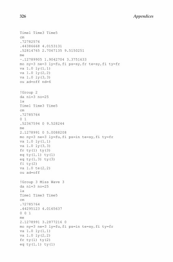
326 Appendices
Time1 Time3 Time5cm.72782576.44386668 4.0153131.52814765 2.7067135 9.5150251me-.12789905 1.9042704 3.3751633mo ny=3 ne=3 ly=fu,fi ps=sy,fr te=sy,fi ty=frva 1.0 ly(1,1)va 1.0 ly(2,2)va 1.0 ly(3,3)ou ad=off nd=6
!Group 2da ni=3 no=25laTime1 Time3 Time5cm.727857640 1.52367594 0 9.528244me2.1278991 0 5.0088208mo ny=3 ne=3 ly=fu,fi ps=in te=sy,fi ty=frva 1.0 ly(1,1)va 1.0 ly(3,3)fr ty(1) ty(3)eq ty(1,1) ty(1)eq ty(1,3) ty(3)fi ty(2)va 1.0 te(2,2)ou ad=off
!Group 3 Miss Wave 3da ni=3 no=25laTime1 Time3 Time5cm.72785764.44295123 4.01656370 0 1me2.1278991 3.2877216 0mo ny=3 ne=3 ly=fu,fi ps=in te=sy,fi ty=frva 1.0 ly(1,1)va 1.0 ly(2,2)fr ty(1) ty(2)eq ty(1,1) ty(1)
Y100315.indb 326 7/15/09 3:00:24 PM

Appendices 327
eq ty(1,2) ty(2)fi ty(3)va 1.0 te(3,3)ou ad=off
!Group 4da ni=3 no=25laTime1 Time3 Time5cm.727857640 10 0 1me2.1278991 0 0mo ny=3 ne=3 ly=fu,fi ps=in te=sy,fi ty=frva 1.0 ly(1,1)fr ty(1)eq ty(1,1) ty(1)fi ty(2) ty(3)va 1.0 te(2,2) te(3,3)ou ad=off
!Study 1 Treatment Group - MCAR (Complete 0% missing)da ni=3 no=75laTime1 Time3 Time5cm.72782576.44386668 4.0153132.52814765 2.7067135 9.5150252me-.12789905 2.2701605 4.1069433mo ny=3 ne=3 ly=fu,fi ps=sy,fr te=sy,fi ty=frva 1.0 ly(1,1)va 1.0 ly(2,2)va 1.0 ly(3,3)ou ad=off!Treatment Groupda ni=3 no=25laTime1 Time3 Time5cm.727857640 1.52367594 0 9.5282441me2.1278991 0 5.7406008
Y100315.indb 327 7/15/09 3:00:24 PM

328 Appendices
mo ny=3 ne=3 ly=fu,fi ps=sy,fr te=sy,fi ty=frva 1.0 ly(1,1)va 1.0 ly(3,3)eq ps(5,1,1) ps(1,1)eq ps(5,2,1) ps(2,1)eq ps(5,2,2) ps(2,2)eq ps(5,3,1) ps(3,1)eq ps(5,3,2) ps(3,2)eq ps(5,3,3) ps(3,3)fr ty(1) ty(3)eq ty(5,1) ty(1)eq ty(5,3) ty(3)fi ty(2)va 1.0 te(2,2)ou ad=off
!Group 3 Tx Miss @ W3!Treatment Groupda ni=3 no=25laTime1 Time3 Time5cm.72785764.44295123 4.01656380 0 1me2.1278991 3.6536116 0mo ny=3 ne=3 ly=fu,fi ps=sy,fr te=sy,fi ty=frva 1.0 ly(1,1)va 1.0 ly(2,2)eq ps(5,1,1) ps(1,1)eq ps(5,2,1) ps(2,1)eq ps(5,2,2) ps(2,2)eq ps(5,3,1) ps(3,1)eq ps(5,3,2) ps(3,2)eq ps(5,3,3) ps(3,3)fr ty(1) ty(2)eq ty(5,1) ty(1)eq ty(5,2) ty(2)fi ty(3)va 1.0 te(3,3)ou ad=off
!Group 8 Treatment Groupda ni=3 no=25laTime1 Time3 Time5cm
Y100315.indb 328 7/15/09 3:00:24 PM

Appendices 329
.727857640 10 0 1me2.1278991 0 0mo ny=3 ne=3 ly=fu,fi ps=sy,fr te=sy,fi ty=frva 1.0 ly(1,1)eq ps(5,1,1) ps(1,1)eq ps(5,2,1) ps(2,1)eq ps(5,2,2) ps(2,2)eq ps(5,3,1) ps(3,1)eq ps(5,3,2) ps(3,2)eq ps(5,3,3) ps(3,3)fr ty(1)eq ty(5,1) ty(1)fi ty(2) ty(3)va 1.0 te(2,2) te(3,3)ou ad=off
MPluS
!Mplus syntax for Model A (MCAR data)TITLE: Chapter 8 - Model A MCAR data;DATA: FILE is GCM_ModelA_MCAR.dat; TYPE IS MEANS COVARIANCE; NGROUPS=4; NOBSERVATION = 25 25 25 25;VARIABLE: NAMES are t1 t3 t5;ANALYSIS: TYPE=MEANSTRUCTURE;MODEL: !Intercept and Slope Loadings; i BY t1@1 t3@1 t5@1; s BY [email protected] [email protected] [email protected] ; !Means for observed variables fixed to 0; [t1-t5@0]; !Error Variance are estimated; t1(1); t3(2); t5(3); !Covariance and variance of intercept and slope are estimated; i with s(4); i(5); s(6);Model G1: !Means for intercept and slope free and equated; [i](7); [s](8);
Y100315.indb 329 7/15/09 3:00:24 PM

330 Appendices
Model G2: !Intercept and Slope Loadings for Group 2; i BY [email protected] [email protected] [email protected]; s BY [email protected] [email protected] [email protected]; !Error variance of t1 and t5 equated to Group 1; t1(1); t5(3); !Error variance of t3 through t5 fixed at 1; t3@1; !Covariance and variance of intercept and slope equated to Group 1; i with s(4); i(5); s(6); !Means for intercept and slope equated to Group 1; [i](7); [s](8); !Means for observed variables fixed to 0; [t1-t5@0];
Model G3: !Intercept and Slope Loading for Group 3; i BY t1@1 t3@1 t5@1; s BY [email protected] [email protected] [email protected] ; !Error variances are estimated; t1(9); t3(10); t5(11); !Covaraince and variance of intercept and slope are estimated; i with s(12); i(13); s(14); !Means for slope is equated to Group 2; [i](15); [s](8); !Means for observed variables fixed to 0; [t1-t5@0];
Model G4: i BY [email protected] [email protected] [email protected]; s BY [email protected] [email protected] [email protected]; !Error Variance of t1 and t2 equated to Group 3; t1(9); t5(11); !Error variance of t3 fixed at 1; t3@1; !Covariance and variance of intercept and slope equated to Group 3; i with s(12); i(13);
Y100315.indb 330 7/15/09 3:00:24 PM

Appendices 331
s(14); !Means for intercept and slope equated to Group 3; [i](15); [s](8); !Means for observed variables fixed to 0; [t1-t5@0];OUTPUT: !For Fmin, see the last value from the function column of TECH5; RESIDUAL TECH1 TECH5;
STaTa
STATA syntax to derive MAR matrices for Pattern Missingness Example#delimit;
set more off;
matrix ly = (1 , 0 \ 1 , 2 \ 1 , 4 );
matrix ps = (1 , .1118 \ .1118, .2 );
matrix te = (1.00 , 0 , 0 \ 0 , 2.27 , 0 \ 0 , 0 , 5.09 );matrix ty = (0 \ 0 \ 0 );*matrix al = (1 \ .798 );matrix al = (1 \ .981 );
matrix w = (1, 0, 0 );
matrix sigma = ly*ps*ly' + te;matrix muy = ty + ly*al;
* Mean of Selection Variable -- Selection on Observed Variables;matrix mus = w*ty;
* Variance of Selection Variable;matrix vars = w*sigma*w';
* Standard Deviation of Selection Variable;matrix sds = cholesky(vars);
Y100315.indb 331 7/15/09 3:00:24 PM

332 Appendices
* Mean and variance in selected subsample (greater than or equal to cutpoint);
matrix d = invnorm(.5);matrix phis = normalden(trace(d));matrix PHIs = normal(trace(d));matrix xPHIs = I(1) - PHIs;
matrix muss = mus + sds*phis*inv(xPHIs);matrix musu = mus - sds*phis*inv(PHIs);matrix varss = vars*(1 + (d*phis*inv(xPHIs)) -(phis*phis*inv(xPHIs)*inv(xPHIs)));matrix varsu = vars*(1 - (d*phis*inv(PHIs)) -(phis*phis*inv(PHIs)*inv(PHIs)));
matrix omegas = inv(vars)*(varss - vars)*inv(vars);matrix omegau = inv(vars)*(varsu - vars)*inv(vars);
matrix sigmas = sigma + omegas*(sigma*(w'*w)*sigma);matrix sigmau = sigma + omegau*(sigma*(w'*w)*sigma);
matrix ks = inv(vars)*(muss - mus);matrix ku = inv(vars)*(musu - mus);
matrix mues = ks*ps*ly’*w';matrix mueu = ku*ps*ly’*w';
matrix muys = muy + ly*mues;matrix muyu = muy + ly*mueu;matrix list sigma;matrix list muy;matrix list sigmas;matrix list muys;matrix list sigmau;matrix list muyu;
STATA syntax for different missing data patterns with MAR data using filter matrix#delimit;* Population Parameters (H0);matrix ly0 = (1, 0 \ 1, 2 \ 1, 4 );matrix ps0 = (1, .1118 \ .1118, .2 );matrix te0 = (1, 0, 0 \ 0, 2.27, 0 \ 0, 0, 5.09 );
Y100315.indb 332 7/15/09 3:00:24 PM

Appendices 333
matrix ty0 = (0 \ 0 \ 0 );matrix al0 = (1 \ .197);
matrix sigma0 = ly0*ps0*ly0' + te0;matrix muy0 = ty0 + ly0*al0;
matrix ly1 = (1, 0 \ 1, 2 \ 1, 4 );matrix ps1 = (1, 0 \ 0, .2 );matrix te1 = (1, 0, 0 \ 0, 2.27, 0 \ 0, 0, 5.09 );matrix ty1 = (0 \ 0 \ 0 );matrix al1 = (1 \ .197 );
matrix sigma1 = ly1*ps1*ly1' + te1;matrix muy1 = ty1 + ly1*al1;
* Create Selected and Unselected Matrices;* Pr(Miss) = f(T1 Only) -- same for both groups here;matrix w = (1, 0, 0 );
* Mean of Selection Variable -- Selection on Observed Variables;matrix mus0 = w*muy0;
* Variance of Selection Variable;matrix vars0 = w*sigma0*w';* Standard Deviation of Selection Variable;matrix sds0 = cholesky(vars0);* Mean and variance in selected subsample (greater than or equal to cutpoint);forvalues probmiss=.05(.05) 1 {;matrix d = invnorm(`probmiss');matrix phis = normalden(trace(d));matrix PHIs = normal(trace(d));matrix xPHIs = I(1) - PHIs;
matrix muss0 = mus0 + sds0*phis*inv(xPHIs);matrix musu0 = mus0 - sds0*phis*inv(PHIs);
matrix varss0 = vars0*(1 + (d*phis*inv(xPHIs)) -(phis*phis*inv(xPHIs)*inv(xPHIs)));matrix varsu0 = vars0*(1 - (d*phis*inv(PHIs)) - (phis*phis*inv(PHIs)*inv(PHIs)));
Y100315.indb 333 7/15/09 3:00:24 PM

334 Appendices
matrix omegas0 = inv(vars0)*(varss0 - vars0)*inv(vars0);matrix omegau0 = inv(vars0)*(varsu0 - vars0)*inv(vars0);
matrix sigmas0 = sigma0 + omegas0*(sigma0*(w'*w)*sigma0);matrix sigmau0 = sigma0 + omegau0*(sigma0*(w'*w)*sigma0);
matrix ks0 = inv(vars0)*(muss0 - mus0);matrix ku0 = inv(vars0)*(musu0 - mus0);
*matrix mues0 = ks0*ps0*ly0'*w';*matrix mueu0 = ku0*ps0*ly0'*w';
*matrix muys0 = muy0 + ly0*mues0;*matrix muyu0 = muy0 + ly0*mueu0;
matrix muys0 = muy0 + sigma0*w'*ks0;matrix muyu0 = muy0 + sigma0*w'*ku0;
* Now Create Appropriate Comparisons;* Original Data;matrix p = rowsof(sigma0);matrix n = (1);matrix fmin= trace(n)*(ln(det(sigma1)) + trace(inv(sigma1)*sigma0) - ln(det(sigma0)) - trace(p) + trace((muy0 - muy1)'*inv(sigma1)*(muy0 - muy1)));
* Complete Data Filter;matrix cfilter = (1, 0, 0 \ 0, 1, 0 \ 0, 0, 1 );* Missing Data Filter;matrix mfilter = (1, 0, 0 \ 0, 1, 0 );* First Compare Selected and Unselected with H1;matrix subsigma0s = cfilter*sigmas0*cfilter';matrix submuy0s = cfilter*muys0;matrix subsigma1c = cfilter*sigma1*cfilter';matrix submuy1c = cfilter*muy1;matrix subsigma0u = mfilter*sigmau0*mfilter';matrix submuy0u = mfilter*muyu0;matrix subsigma1m = mfilter*sigma1*mfilter';matrix submuy1m = mfilter*muy1;matrix subpc = rowsof(subsigma0s);matrix nc = (1 - `probmiss');matrix subpm = rowsof(subsigma0u);matrix nm = (`probmiss');
Y100315.indb 334 7/15/09 3:00:24 PM

Appendices 335
matrix fminc1 = trace(nc)*(ln(det(subsigma1c)) + trace(inv(subsigma1c)*subsigma0s) - ln(det(subsigma0s)) - trace(subpc) + trace((submuy0s - submuy1c)'*inv(subsigma1c)*(submuy0s - submuy1c)));
matrix fminm1 = trace(nm)*(ln(det(subsigma1m)) + trace(inv(subsigma1m)*subsigma0u) - ln(det(subsigma0u)) - trace(subpm) + trace((submuy0u - submuy1m)'*inv(subsigma1m)*(submuy0u - submuy1m)));
* Next Compare Selected and Unselected with H0 (0 under MCAR);matrix subsigma0c = cfilter*sigma0*cfilter';matrix submuy0c = cfilter*muy0;matrix subsigma0m = mfilter*sigma0*mfilter';matrix submuy0m = mfilter*muy0;
matrix fminc0 = trace(nc)*(ln(det(subsigma0c)) + trace(inv(subsigma0c)*subsigma0s) - ln(det(subsigma0s)) - trace(subpc) + trace((submuy0s - submuy0c)'*inv(subsigma0c)*(submuy0s - submuy0c)));
matrix fminm0 = trace(nm)*(ln(det(subsigma0m)) + trace(inv(subsigma0m)*subsigma0u) - ln(det(subsigma0u)) - trace(subpm) + trace((submuy0u - submuy0m)'*inv(subsigma0m)*(submuy0u - submuy0m)));
* Incomplete Data;* Complete;* Missing;matrix fminall = (fminc1 + fminm1) - (fminc0 + fminm0);matrix list fminc1;matrix list fminc0;matrix list fminm1;matrix list fminm0;matrix list fminall;
matrix pctfmin = 100*fminall*inv(fmin);mat list pctfmin;};
Chapter 9 Appendix
STaTa
/* Chapter 9 Example Generating Non-Normal Univariate Variables*/
Y100315.indb 335 7/15/09 3:00:24 PM
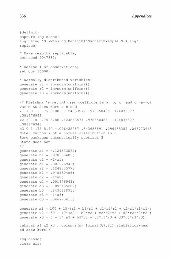
336 Appendices
#delimit;capture log close;log using "G:\Missing Data\LEA\Syntax\Example 9-A.log", replace;
* Make results replicable;set seed 2047881;
* Define # of observations;set obs 10000;
* Normally distributed variables;generate r1 = invnorm(uniform());generate r2 = invnorm(uniform());generate r3 = invnorm(uniform());
/* Fleishman’s method uses coefficients a, b, c, and d (a=-c)Var M SD Skew Kurt a b c dx1 100 15 .75 3.80 -.124833577 .978350485 .124833577 .001976943x2 50 10 -.75 3.80 .124833577 .978350485 -.124833577 .001976943x3 0 1 .75 5.40 -.096435287 .843688891 .096435287 .046773413Note: Kurtosis of a normal distribution is 3Some packages automatically subtract 3Stata does not*/generate a1 = -.124833577;generate b1 = .978350485;generate c1 = -1*a1;generate d1 = .001976943;generate a2 = .124833577;generate b2 = .978350485;generate c2 = -1*a2;generate d2 = .001976943;generate a3 = -.096435287;generate b3 = .843688891;generate c3 = -1*a3;generate d3 = .046773413;
generate x1 = 100 + 15*(a1 + b1*r1 + c1*r1*r1 + d1*r1*r1*r1);generate x2 = 50 + 10*(a2 + b2*r2 + c2*r2*r2 + d2*r2*r2*r2);generate x3 = 0 + 1*(a3 + b3*r3 + c3*r3*r3 + d3*r3*r3*r3);
tabstat x1 x2 x3 , columns(s) format(%9.2f) statistics(mean sd skew kurt);
log close;clear all;
Y100315.indb 336 7/15/09 3:00:25 PM

Appendices 337
Solving for Fleishman’s Coefficients
/* Chapter 9 Example Solving for Fleishman’s Coefficients*/#delimit;capture log close;*log using "G:\Missing Data\LEA\Syntax\Example 9-C.log", replace;mat maxiter = (500);mat iter = (0);* Skewness and Kurtosis;mat skewkurt = (1, 5 \ 2, 7 \ 0, 0 \ -2, 7); mat skew = skewkurt[1..rowsof(skewkurt),1];mat kurt = skewkurt[1..rowsof(skewkurt),2];mat output = J(rowsof(skewkurt),3,0);mat coef = (1 \ 0 \ 0);mat f = J(3,1,1);while trace(iter) <= trace(maxiter) & max(abs(f[1,1]),abs(f[2,1]),abs(f[3,1])) > .000001 {;mat x1 = coef[1,1];mat x2 = coef[2,1];mat x3 = coef[3,1];
mat f = (x1*x1+6*x1*x3+2*x2*x2+15*x3*x3 - 1 \ 2*x2*(x1*x1+24*x1*x3+105*x3*x3+2) - skew[4,1] \ 24*(x1*x3+x2*x2*(1+x1*x1+28*x1*x3)+x3*x3*(12+48*x1*x3+141*x2*x2+225*x3*x3)) - kurt[4,1]);
mat j = (2*x1+6*x3, 4*x2, 6*x1+30*x3 \ 4*x2*(x1+12*x3), 2*(x1*x1+24*x1*x3+105*x3*x3+2), 4*x2*(12*x1+105*x3) \ 24*(x3+x2*x2*(2*x1+28*x3)+48*x3*x3), 48*x2*(1+x1*x1+28*x1*x3+141*x3*x3),
24*(x1+28*x1*x2*x2+2*x3*(12+48*x1*x3+141*x2*x2+225*x3*x3)+x3*x3)+x3*x3*(48*x1+450*x3));
mat delta = -1*inv(j)*f;mat coef = coef + delta;mat iter=iter+I(1);};mat list iter;mat list coef;mat list delta;mat list f;mat list j;
Y100315.indb 337 7/15/09 3:00:25 PM

338 Appendices
set obs 10000;set seed 2047881;gen u = invnorm(uniform());
gen x = .57256304 + .8489756*u -.57256304*u*u -.10867268*u*u*u;gen y = -.2600226 -.76158527*u -.2600226*u*u -.05307227*u*u*u;
tabstat x y, columns(statistics) statistics (mean sd skew kurt);
generating Non‑Normally Distributed Multivariate Data
/* This program calculates the intermediate correlation needed to generate pairs of non-normal variates with a specified target correlation*/#delimit;capture log close;log using "G:\Missing Data\LEA\Syntax\Example 9-D.log", replace;
set obs 1;gen b1 = .978350485;gen c1 = -.124833577;gen d1 = .001976943;
gen b2 = .978350485;gen c2 = .124833577;gen d2 = .001976943;
gen target = .7;gen r = .2;gen f = 0;gen df = 0;gen rtemp = 0;gen ratio = 0;
quietly forvalues i=1/50 {;replace f = (r^3*6*d1*d2+r^2*2*c1*c2+r*(b1*b2+3*b1*d2+3*d1*b2+9*d1*d2)-target);replace df = (3*r^2*6*d1*d2+2*r^2*c1*c2+(b1*b2+3*b1*d2+3*d1*b2+9*d1*d2));replace ratio = f/df;quietly replace rtemp = r - ratio;
Y100315.indb 338 7/15/09 3:00:25 PM
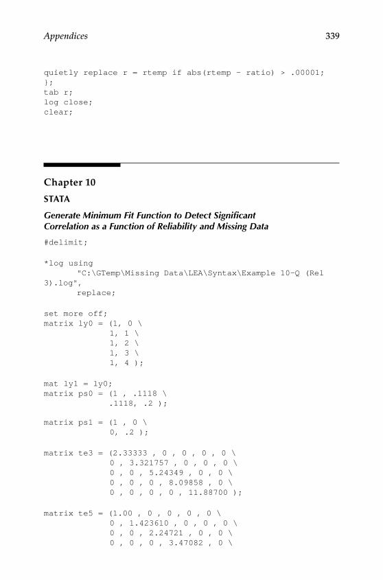
Appendices 339
quietly replace r = rtemp if abs(rtemp - ratio) > .00001;};tab r;log close;clear;
Chapter 10
STaTa
Generate Minimum Fit Function to Detect Significant Correlation as a Function of Reliability and Missing Data
#delimit;
*log using "C:\GTemp\Missing Data\LEA\Syntax\Example 10-Q (Rel 3).log", replace;
set more off;matrix ly0 = (1, 0 \ 1, 1 \ 1, 2 \ 1, 3 \ 1, 4 );
mat ly1 = ly0;matrix ps0 = (1 , .1118 \ .1118, .2 );
matrix ps1 = (1 , 0 \ 0, .2 );
matrix te3 = (2.33333 , 0 , 0 , 0 , 0 \ 0 , 3.321757 , 0 , 0 , 0 \ 0 , 0 , 5.24349 , 0 , 0 \ 0 , 0 , 0 , 8.09858 , 0 \ 0 , 0 , 0 , 0 , 11.88700 );
matrix te5 = (1.00 , 0 , 0 , 0 , 0 \ 0 , 1.423610 , 0 , 0 , 0 \ 0 , 0 , 2.24721 , 0 , 0 \ 0 , 0 , 0 , 3.47082 , 0 \
Y100315.indb 339 7/15/09 3:00:25 PM

340 Appendices
0 , 0 , 0 , 0 , 5.094430 );matrix te7 = (0.42857 , 0 , 0 , 0 , 0 \ 0 , 0.610119 , 0 , 0 , 0 \ 0 , 0 , 0.96309 , 0 , 0 \ 0 , 0 , 0 , 1.48749 , 0 \ 0 , 0 , 0 , 0 , 2.183327 );
mat te0 = te3; *change to te5 or te7 depending on Reliability needed;mat te1 = te0;
matrix ty0 = (0 \ 0 \ 0 \ 0 \ 0 );matrix al0 = (1 \ .981 );
matrix ty1 = (0 \ 0 \ 0 \ 0 \ 0 );matrix al1 = (1 \ .981 );
matrix sigma0 = ly0*ps0*ly0' + te0;matrix muy0 = ty0 + ly0*al0;
matrix sigma1 = ly1*ps1*ly1' + te1;matrix muy1 = ty1 + ly1*al1;
* Create Selected and Unselected Matrices;* Pr(Miss) = f1 Only;matrix w = (2, 1, 0, 0, 0);* Mean of Selection Variable -- Selection on Observed Variables;matrix mus0 = w*muy0;
* Variance of Selection Variable;matrix vars0 = w*sigma0*w';
* Standard Deviation of Selection Variable;matrix sds0 = cholesky(vars0);
* Mean and variance in selected subsample (greater than or equal to cutpoint);forvalues probmiss=.05(.05) 1 {;matrix d = invnorm(`probmiss');matrix phis = normalden(trace(d));matrix PHIs = normal(trace(d));matrix xPHIs = I(1) - PHIs;matrix muss0 = mus0 + sds0*phis*inv(xPHIs);matrix musu0 = mus0 - sds0*phis*inv(PHIs);
matrix varss0 = vars0*(1 + (d*phis*inv(xPHIs)) -(phis*phis*inv(xPHIs)*inv(xPHIs)));
Y100315.indb 340 7/15/09 3:00:25 PM

Appendices 341
matrix varsu0 = vars0*(1 - (d*phis*inv(PHIs)) -(phis*phis*inv(PHIs)*inv(PHIs)));
matrix omegas0 = inv(vars0)*(varss0 - vars0)*inv(vars0);matrix omegau0 = inv(vars0)*(varsu0 - vars0)*inv(vars0);
matrix sigmas0 = sigma0 + omegas0*(sigma0*(w’*w)*sigma0);matrix sigmau0 = sigma0 + omegau0*(sigma0*(w’*w)*sigma0);
matrix ks0 = inv(vars0)*(muss0 - mus0);matrix ku0 = inv(vars0)*(musu0 - mus0);
*matrix mues0 = ks0*ps0*ly0'*w';*matrix mueu0 = ku0*ps0*ly0'*w';
*matrix muys0 = muy0 + ly0*mues0;*matrix muyu0 = muy0 + ly0*mueu0;
matrix muys0 = muy0 + sigma0*w’*ks0;matrix muyu0 = muy0 + sigma0*w’*ku0;
* Now Create Appropriate Comparisons;* Original Data;matrix p = rowsof(sigma0);matrix n = (1);matrix fmin= trace(n)*(ln(det(sigma1)) + trace(inv(sigma1)*sigma0) - ln(det(sigma0)) - trace(p) + trace((muy0 - muy1)'*inv(sigma1)*(muy0 - muy1)));
* Complete Data Filter;matrix cfilter = I(5);
* Missing Data Filter;matrix mfilter = (1, 0, 0, 0, 0 \ 0, 1, 0, 0, 0 );
* First Compare Selected and Unselected with H1;matrix subsigma0s = cfilter*sigmas0*cfilter';matrix submuy0s = cfilter*muys0;matrix subsigma1c = cfilter*sigma1*cfilter';matrix submuy1c = cfilter*muy1;matrix subsigma0u = mfilter*sigmau0*mfilter';matrix submuy0u = mfilter*muyu0;matrix subsigma1m = mfilter*sigma1*mfilter';matrix submuy1m = mfilter*muy1;matrix subpc = rowsof(subsigma0s);matrix nc = (1 - `probmiss');
Y100315.indb 341 7/15/09 3:00:25 PM

342 Appendices
matrix subpm = rowsof(subsigma0u);matrix nm = (`probmiss');
matrix fminc1 = trace(nc)*(ln(det(subsigma1c)) + trace(inv(subsigma1c)*subsigma0s) - ln(det(subsigma0s)) - trace(subpc) + trace((submuy0s - submuy1c)’*inv(subsigma1c)*(submuy0s - submuy1c)));
matrix fminm1 = trace(nm)*(ln(det(subsigma1m)) + trace(inv(subsigma1m)*subsigma0u) - ln(det(subsigma0u)) - trace(subpm) + trace((submuy0u - submuy1m)'*inv(subsigma1m)*(submuy0u - submuy1m)));
* Next Compare Selected and Unselected with H0 (0 under MCAR);matrix subsigma0c = cfilter*sigma0*cfilter';matrix submuy0c = cfilter*muy0;matrix subsigma0m = mfilter*sigma0*mfilter';matrix submuy0m = mfilter*muy0;
matrix fminc0 = trace(nc)*(ln(det(subsigma0c)) + trace(inv(subsigma0c)*subsigma0s) - ln(det(subsigma0s)) - trace(subpc) + trace((submuy0s - submuy0c)'*inv(subsigma0c)*(submuy0s - submuy0c)));
matrix fminm0 = trace(nm)*(ln(det(subsigma0m)) + trace(inv(subsigma0m)*subsigma0u) - ln(det(subsigma0u)) - trace(subpm) + trace((submuy0u - submuy0m)'*inv(subsigma0m)*(submuy0u - submuy0m)));
* Incomplete Data;* Complete;* Missing;matrix fminall = (fminc1 + fminm1) - (fminc0 + fminm0);
matrix list PHIs, noheader nonames;*matrix list fminc1;*matrix list fminc0;*matrix list fminm1;*matrix list fminm0;matrix list fminall, noheader nonames;*matrix pctfmin = 100*fminall*inv(fmin);*mat list pctfmin;};mat list fmin, noheader nonames;
*log close;
Y100315.indb 342 7/15/09 3:00:25 PM

Appendices 343
Calculate Power for the Models as a Function of Reliability and Missing Data#delimit;
capture drop df alpha n power*;
gen df=1;gen alpha = .05;gen n = 500;gen power3 = 1 - nchi2(df,(n-1)*ncp3,invchi2tail(df,alpha));gen power5 = 1 - nchi2(df,(n-1)*ncp5,invchi2tail(df,alpha));gen power7 = 1 - nchi2(df,(n-1)*ncp7,invchi2tail(df,alpha));
STaTa
STATA Code to Generate the Covariance Matrices and Mean Vectors for MAR Data with Auxiliary Variable of 0.1 Correlation with Pre-test Data
For Control Group:
#delimit;set mem 200m;capture log close;
/*Save the output */log using "c:\study2\covariates\control_0.1 covariate.log", replace;/*Define Covariance Matrix *//*Curran & Muthen, 1999 *//*Control Group Matrix*/
/*Auxiliary variable correlated at 0.1 with Time 1 Data*/matrix S4 = (2.0000000, 1.1118034, 1.2236068, 1.3354102, 1.4472136, 0.1414200\1.1118034, 2.8472136, 1.7354102, 2.0472136, 2.3590170, 0.0000000\1.2236068, 1.7354102, 4.4944272, 2.7590170, 3.2708204, 0.0000000\1.3354102, 2.0472136, 2.7590170, 6.9416408, 4.1826238, 0.0000000\1.4472136, 2.3590170, 3.2708204, 4.1826238, 10.188854, 0.0000000\0.1414200, 0.0000000, 0.0000000, 0.0000000, 00.000000, 1.0000000);
matrix M4 = (1.00000, 1.797998, 2.595996, 3.393994, 4.191992, 0.000000);
Y100315.indb 343 7/15/09 3:00:25 PM

344 Appendices
/*Set Replicable See*/set seed 1234567;
/*Generate a 1,000,000 Observation Dataset*//* 5 Waves of Data*/corr2data t1-t5 cov, n(1000000) cov(S4) means(M4);
/*Establish a selection variable to make MAR data *//*Weighted on Time1 (Pretest) score only */generate scrit01 = -1*t1;
/*Sort Cases by values on selection variable *//*Note that this is like the phenotypic (i.e., observed variable) sorting of Dolan */sort scrit01;
/*Now determine extent of MAR missing data*//*First initialize variables*/generate sel00 = 0;generate sel05 = 0;generate sel10 = 0;generate sel15 = 0;generate sel20 = 0;generate sel25 = 0;generate sel30 = 0;generate sel35 = 0;generate sel40 = 0;generate sel45 = 0;generate sel50 = 0;generate sel55 = 0;generate sel60 = 0;generate sel65 = 0;generate sel70 = 0;generate sel75 = 0;generate sel80 = 0;generate sel85 = 0;generate sel90 = 0;generate sel95 = 0;
/*Then make groups representing different proportions of missing data */replace sel05=1 if _n <= 50000;replace sel10=1 if _n <= 100000;replace sel15=1 if _n <= 150000;replace sel20=1 if _n <= 200000;replace sel25=1 if _n <= 250000;replace sel30=1 if _n <= 300000;replace sel35=1 if _n <= 350000;
Y100315.indb 344 7/15/09 3:00:25 PM

Appendices 345
replace sel40=1 if _n <= 400000;replace sel45=1 if _n <= 450000;replace sel50=1 if _n <= 500000;replace sel55=1 if _n <= 550000;replace sel60=1 if _n <= 600000;replace sel65=1 if _n <= 650000;replace sel70=1 if _n <= 700000;replace sel75=1 if _n <= 750000;replace sel80=1 if _n <= 800000;replace sel85=1 if _n <= 850000;replace sel90=1 if _n <= 900000;replace sel95=1 if _n <= 950000;
/*Now we make and store some matrices by group *//* 5% Missing */matrix accum c05 = t1-t5 cov if sel05==0, means(mc05) dev noconst;matrix accum m05 = t1-t5 cov if sel05==1, means(mm05) dev noconst;
/* 10% Missing */matrix accum c10 = t1-t5 cov if sel10==0, means(mc10) dev noconst;matrix accum m10 = t1-t5 cov if sel10==1, means(mm10) dev noconst;
/* 15% Missing */matrix accum c15 = t1-t5 cov if sel15==0, means(mc15) dev noconst;matrix accum m15 = t1-t5 cov if sel15==1, means(mm15) dev noconst;
/* 20% Missing */matrix accum c20 = t1-t5 cov if sel20==0, means(mc20) dev noconst;matrix accum m20 = t1-t5 cov if sel20==1, means(mm20) dev noconst;
/* 25% Missing */matrix accum c25 = t1-t5 cov if sel25==0, means(mc25) dev noconst;matrix accum m25 = t1-t5 cov if sel25==1, means(mm25) dev noconst;
/* 30% Missing */matrix accum c30 = t1-t5 cov if sel30==0, means(mc30) dev noconst;
Y100315.indb 345 7/15/09 3:00:25 PM

346 Appendices
matrix accum m30 = t1-t5 cov if sel30==1, means(mm30) dev noconst;
/* 35% Missing */matrix accum c35 = t1-t5 cov if sel35==0, means(mc35) dev noconst;matrix accum m35 = t1-t5 cov if sel35==1, means(mm35) dev noconst;
/* 40% Missing */matrix accum c40 = t1-t5 cov if sel40==0, means(mc40) dev noconst;matrix accum m40 = t1-t5 cov if sel40==1, means(mm40) dev noconst;
/* 45% Missing */matrix accum c45 = t1-t5 cov if sel45==0, means(mc45) dev noconst;matrix accum m45 = t1-t5 cov if sel45==1, means(mm45) dev noconst;
/* 50% Missing */matrix accum c50 = t1-t5 cov if sel50==0, means(mc50) dev noconst;matrix accum m50 = t1-t5 cov if sel50==1, means(mm50) dev noconst;
/* 55% Missing */matrix accum c55 = t1-t5 cov if sel55==0, means(mc55) dev noconst;matrix accum m55 = t1-t5 cov if sel55==1, means(mm55) dev noconst;
/* 60% Missing */matrix accum c60 = t1-t5 cov if sel60==0, means(mc60) dev noconst;matrix accum m60 = t1-t5 cov if sel60==1, means(mm60) dev noconst;
/* 65% Missing */matrix accum c65 = t1-t5 cov if sel65==0, means(mc65) dev noconst;matrix accum m65 = t1-t5 cov if sel65==1, means(mm65) dev noconst;
/* 70% Missing */matrix accum c70 = t1-t5 cov if sel70==0, means(mc70) dev noconst;
Y100315.indb 346 7/15/09 3:00:25 PM

Appendices 347
matrix accum m70 = t1-t5 cov if sel70==1, means(mm70) dev noconst;
/* 75% Missing */matrix accum c75 = t1-t5 cov if sel75==0, means(mc75) dev noconst;matrix accum m75 = t1-t5 cov if sel75==1, means(mm75) dev noconst;
/* 80% Missing */matrix accum c80 = t1-t5 cov if sel80==0, means(mc80) dev noconst;matrix accum m80 = t1-t5 cov if sel80==1, means(mm80) dev noconst;
/* 85% Missing */matrix accum c85 = t1-t5 cov if sel85==0, means(mc85) dev noconst;matrix accum m85 = t1-t5 cov if sel85==1, means(mm85) dev noconst;
/* 90% Missing */matrix accum c90 = t1-t5 cov if sel90==0, means(mc90) dev noconst;matrix accum m90 = t1-t5 cov if sel90==1, means(mm90) dev noconst;
/* 95% Missing */matrix accum c95 = t1-t5 cov if sel95==0, means(mc95) dev noconst;matrix accum m95 = t1-t5 cov if sel95==1, means(mm95) dev noconst;
/*Make Covariance Matrix by Dividing by Sample Size */matrix c05=c05/950000;matrix m05=m05/50000;matrix c10=c10/900000;matrix m10=m10/100000;matrix c15=c15/850000;matrix m15=m15/150000;matrix c20=c20/800000;matrix m20=m20/200000;matrix c25=c25/750000;matrix m25=m25/250000;matrix c30=c30/700000;matrix m30=m30/300000;matrix c35=c35/650000;matrix m35=m35/350000;
Y100315.indb 347 7/15/09 3:00:25 PM

348 Appendices
matrix c40=c40/600000;matrix m40=m40/400000;matrix c45=c45/550000;matrix m45=m45/450000;matrix c50=c50/500000;matrix m50=m50/500000;matrix c55=c55/450000;matrix m55=m55/550000;matrix c60=c60/400000;matrix m60=m60/600000;matrix c65=c65/350000;matrix m65=m65/650000;matrix c70=c70/300000;matrix m70=m70/700000;matrix c75=c75/250000;matrix m75=m75/750000;matrix c80=c80/200000;matrix m80=m80/800000;matrix c85=c85/150000;matrix m85=m85/850000;matrix c90=c90/100000;matrix m90=m90/900000;matrix c95=c95/50000;matrix m95=m95/950000;
/*Print the Output*/matrix list c05;matrix list mc05;matrix list m05;matrix list mm05;matrix list c10;matrix list mc10;matrix list m10;matrix list mm10;matrix list c15;matrix list mc15;matrix list m15;matrix list mm15;matrix list c20;matrix list mc20;matrix list m20;matrix list mm20;matrix list c25;matrix list mc25;matrix list m25;matrix list mm25;matrix list c30;matrix list mc30;
Y100315.indb 348 7/15/09 3:00:25 PM

Appendices 349
matrix list m30;matrix list mm30;matrix list c35;matrix list mc35;matrix list m35;matrix list mm35;matrix list c40;matrix list mc40;matrix list m40;matrix list mm40;matrix list c45;matrix list mc45;matrix list m45;matrix list mm45;matrix list c50;matrix list mc50;matrix list m50;matrix list mm50;matrix list c55;matrix list mc55;matrix list m55;matrix list mm55;matrix list c60;matrix list mc60;matrix list m60;matrix list mm60;matrix list c65;matrix list mc65;matrix list m65;matrix list mm65;matrix list c70;matrix list mc70;matrix list m70;matrix list mm70;matrix list c75;matrix list mc75;matrix list m75;matrix list mm75;matrix list c80;matrix list mc80;matrix list m80;matrix list mm80;matrix list c85;matrix list mc85;matrix list m85;matrix list mm85;matrix list c90;matrix list mc90;
Y100315.indb 349 7/15/09 3:00:25 PM

350 Appendices
matrix list m90;matrix list mm90;matrix list c95;matrix list mc95;matrix list m95;matrix list mm95;
corr t1 t2 t3 t4 t5 cov, m c;
log close;clear;
For Treatment Group:
#delimit;set mem 200m;capture log close;
/*Save the output */log using "c:\study2\covariates\Treatment_0.1 Covariate.log", replace;
/*Define Covariance Matrix *//*Curran & Muthen, 1999 *//*Treatment Group Matrix*/
matrix S4 = (2.0000000, 1.1118034, 1.2236068, 1.3354102, 1.4472136, 0.1414200\1.1118034, 2.8472136, 1.7354102, 2.0472136, 2.3590170, 0.0000000\1.2236068, 1.7354102, 4.4944272, 2.7590170, 3.2708204, 0.0000000\1.3354102, 2.0472136, 2.7590170, 6.9416408, 4.1826238, 0.0000000\1.4472136, 2.3590170, 3.2708204, 4.1826238, 10.188854, 0.0000000\0.1414200, 0.0000000, 0.0000000, 0.0000000, 00.000000, 1.0000000);matrix M4 = (1.0000000, 1.9809430, 2.9618860, 3.9428290, 4.9237720, 0.0000000);
/*Set Replicable Seed*/set seed 1234567;
/*Generate a 1,000,000 Observation Dataset*/
Y100315.indb 350 7/15/09 3:00:25 PM

Appendices 351
/* 5 Waves of Data & Covariance*/corr2data t1-t5 cov, n(1000000) cov(S4) means(M4);
/*Establish a selection variable to make MAR data *//*Weighted on Time1 (Pretest) score only */generate scrit01 = -1*t1;
/*Sort Cases by values on selection variable *//*Note that this is like the phenotypic (i.e., observed variable) sorting of Dolan */sort scrit01;
/*Now determine extent of MAR missing data*//*First initialize variables*/generate sel00 = 0;generate sel05 = 0;generate sel10 = 0;generate sel15 = 0;generate sel20 = 0;generate sel25 = 0;generate sel30 = 0;generate sel35 = 0;generate sel40 = 0;generate sel45 = 0;generate sel50 = 0;generate sel55 = 0;generate sel60 = 0;generate sel65 = 0;generate sel70 = 0;generate sel75 = 0;generate sel80 = 0;generate sel85 = 0;generate sel90 = 0;generate sel95 = 0;
/*Then make groups representing different proportions of missing data */replace sel05=1 if _n <= 50000;replace sel10=1 if _n <= 100000;replace sel15=1 if _n <= 150000;replace sel20=1 if _n <= 200000;replace sel25=1 if _n <= 250000;replace sel30=1 if _n <= 300000;replace sel35=1 if _n <= 350000;replace sel40=1 if _n <= 400000;replace sel45=1 if _n <= 450000;replace sel50=1 if _n <= 500000;replace sel55=1 if _n <= 550000;
Y100315.indb 351 7/15/09 3:00:25 PM

352 Appendices
replace sel60=1 if _n <= 600000;replace sel65=1 if _n <= 650000;replace sel70=1 if _n <= 700000;replace sel75=1 if _n <= 750000;replace sel80=1 if _n <= 800000;replace sel85=1 if _n <= 850000;replace sel90=1 if _n <= 900000;replace sel95=1 if _n <= 950000;
/*Now we make and store some matrices by group *//* 5% Missing */matrix accum c05 = t1-t5 cov if sel05==0, means(mc05) dev noconst;matrix accum m05 = t1-t5 cov if sel05==1, means(mm05) dev noconst;
/* 10% Missing */matrix accum c10 = t1-t5 cov if sel10==0, means(mc10) dev noconst;matrix accum m10 = t1-t5 cov if sel10==1, means(mm10) dev noconst;
/* 15% Missing */matrix accum c15 = t1-t5 cov if sel15==0, means(mc15) dev noconst;matrix accum m15 = t1-t5 cov if sel15==1, means(mm15) dev noconst;
/* 20% Missing */matrix accum c20 = t1-t5 cov if sel20==0, means(mc20) dev noconst;matrix accum m20 = t1-t5 cov if sel20==1, means(mm20) dev noconst;
/* 25% Missing */matrix accum c25 = t1-t5 cov if sel25==0, means(mc25) dev noconst;matrix accum m25 = t1-t5 cov if sel25==1, means(mm25) dev noconst;
/* 30% Missing */matrix accum c30 = t1-t5 cov if sel30==0, means(mc30) dev noconst;matrix accum m30 = t1-t5 cov if sel30==1, means(mm30) dev noconst;
Y100315.indb 352 7/15/09 3:00:25 PM

Appendices 353
/* 35% Missing */matrix accum c35 = t1-t5 cov if sel35==0, means(mc35) dev noconst;matrix accum m35 = t1-t5 cov if sel35==1, means(mm35) dev noconst;
/* 40% Missing */matrix accum c40 = t1-t5 cov if sel40==0, means(mc40) dev noconst;matrix accum m40 = t1-t5 cov if sel40==1, means(mm40) dev noconst;
/* 45% Missing */matrix accum c45 = t1-t5 cov if sel45==0, means(mc45) dev noconst;matrix accum m45 = t1-t5 cov if sel45==1, means(mm45) dev noconst;
/* 50% Missing */matrix accum c50 = t1-t5 cov if sel50==0, means(mc50) dev noconst;matrix accum m50 = t1-t5 cov if sel50==1, means(mm50) dev noconst;
/* 55% Missing */matrix accum c55 = t1-t5 cov if sel55==0, means(mc55) dev noconst;matrix accum m55 = t1-t5 cov if sel55==1, means(mm55) dev noconst;
/* 60% Missing */matrix accum c60 = t1-t5 cov if sel60==0, means(mc60) dev noconst;matrix accum m60 = t1-t5 cov if sel60==1, means(mm60) dev noconst;
/* 65% Missing */matrix accum c65 = t1-t5 cov if sel65==0, means(mc65) dev noconst;matrix accum m65 = t1-t5 cov if sel65==1, means(mm65) dev noconst;
/* 70% Missing */matrix accum c70 = t1-t5 cov if sel70==0, means(mc70) dev noconst;matrix accum m70 = t1-t5 cov if sel70==1, means(mm70) dev noconst;
Y100315.indb 353 7/15/09 3:00:25 PM

354 Appendices
/* 75% Missing */matrix accum c75 = t1-t5 cov if sel75==0, means(mc75) dev noconst;matrix accum m75 = t1-t5 cov if sel75==1, means(mm75) dev noconst;
/* 80% Missing */matrix accum c80 = t1-t5 cov if sel80==0, means(mc80) dev noconst;matrix accum m80 = t1-t5 cov if sel80==1, means(mm80) dev noconst;
/* 85% Missing */matrix accum c85 = t1-t5 cov if sel85==0, means(mc85) dev noconst;matrix accum m85 = t1-t5 cov if sel85==1, means(mm85) dev noconst;
/* 90% Missing */matrix accum c90 = t1-t5 cov if sel90==0, means(mc90) dev noconst;matrix accum m90 = t1-t5 cov if sel90==1, means(mm90) dev noconst;
/* 95% Missing */matrix accum c95 = t1-t5 cov if sel95==0, means(mc95) dev noconst;matrix accum m95 = t1-t5 cov if sel95==1, means(mm95) dev noconst;
/*Make Covariance Matrix by Dividing by Sample Size */matrix c05=c05/950000;matrix m05=m05/50000;matrix c10=c10/900000;matrix m10=m10/100000;matrix c15=c15/850000;matrix m15=m15/150000;matrix c20=c20/800000;matrix m20=m20/200000;matrix c25=c25/750000;matrix m25=m25/250000;matrix c30=c30/700000;matrix m30=m30/300000;matrix c35=c35/650000;matrix m35=m35/350000;
Y100315.indb 354 7/15/09 3:00:26 PM

Appendices 355
matrix c40=c40/600000;matrix m40=m40/400000;matrix c45=c45/550000;matrix m45=m45/450000;matrix c50=c50/500000;matrix m50=m50/500000;matrix c55=c55/450000;matrix m55=m55/550000;matrix c60=c60/400000;matrix m60=m60/600000;matrix c65=c65/350000;matrix m65=m65/650000;matrix c70=c70/300000;matrix m70=m70/700000;matrix c75=c75/250000;matrix m75=m75/750000;matrix c80=c80/200000;matrix m80=m80/800000;matrix c85=c85/150000;matrix m85=m85/850000;matrix c90=c90/100000;matrix m90=m90/900000;matrix c95=c95/50000;matrix m95=m95/950000;
/*Print the Output*/matrix list c05;matrix list mc05;matrix list m05;matrix list mm05;matrix list c10;matrix list mc10;matrix list m10;matrix list mm10;matrix list c15;matrix list mc15;matrix list m15;matrix list mm15;matrix list c20;matrix list mc20;matrix list m20;matrix list mm20;matrix list c25;matrix list mc25;matrix list m25;matrix list mm25;matrix list c30;
Y100315.indb 355 7/15/09 3:00:26 PM

356 Appendices
matrix list mc30;matrix list m30;matrix list mm30;matrix list c35;matrix list mc35;matrix list m35;matrix list mm35;matrix list c40;matrix list mc40;matrix list m40;matrix list mm40;matrix list c45;matrix list mc45;matrix list m45;matrix list mm45;matrix list c50;matrix list mc50;matrix list m50;matrix list mm50;matrix list c55;matrix list mc55;matrix list m55;matrix list mm55;matrix list c60;matrix list mc60;matrix list m60;matrix list mm60;matrix list c65;matrix list mc65;matrix list m65;matrix list mm65;matrix list c70;matrix list mc70;matrix list m70;matrix list mm70;matrix list c75;matrix list mc75;matrix list m75;matrix list mm75;matrix list c80;matrix list mc80;matrix list m80;matrix list mm80;matrix list c85;matrix list mc85;matrix list m85;
Y100315.indb 356 7/15/09 3:00:26 PM

Appendices 357
matrix list mm85;matrix list c90;matrix list mc90;matrix list m90;matrix list mm90;matrix list c95;matrix list mc95;matrix list m95;matrix list mm95;
corr t1 t2 t3 t4 t5 cov, m c;log close;clear;
Y100315.indb 357 7/15/09 3:00:26 PM

Y100315.indb 358 7/15/09 3:00:26 PM

359
Name Index
A
Abadir, K. M. 22Abraham, W. T. 18, 80Acock, A. C. 2Allison, P. D. 2, 47, 56, 61, 65, 106Alpert. A.120Altman, D. 14Anderson, E. R. 144Anderson, J. C. 41, 168Anderson, T. W. 47, 53Arbuckle, J. L. 21, 47, 53, 168Arvey, R. D. 121, 211
B
Balla, J. R. 42Bandalos, D. L. 167, 168, 170, 178, 179,
180, 181, 182, 191Bell, R. Q. 3, 143, 144Bennett, N. 41Bentler, P. M. 21, 41, 42, 43, 53, 168, 208Bierman, K. 121, 143Boker, S. M. 21Bollen, K. A. 21, 22, 29, 43, 92, 168, 169,
170, 180, 190, 191Bonnett, D. G. 42Boomsma, A. 43Boomsma, D. I. 102Brown, C. H. 232, 233Browne, M. W. 43, 72, 73, 75, 80, 211Bryk, A. S. 120Buchner, A. 81Burr, I. W. 174, 178Byrne, B. M. 21, 43
C
Cai., L. 75, 80, 211Campbell, D. T. 3, 143Chan, W. S. 3, 119Chen, F. 92, 168, 169, 170, 180, 190, 191
Cleary, T. A. 211Cohen, J. H. 2, 9, 10, 18Cole, D. A. 121, 211Collins, L. M. 121, 143Cudeck. R. 43Cumsille, P. E. 48, 144, 147, 152, 164Curran, P. J. 92, 120, 122, 141, 145, 146,
168, 169, 170, 180, 190, 191
D
Davey, A. 55, 103, 141, 144, 179, 180, 182, 207, 208, 209, 210, 219
Davey Smith, G. 14Dempster, A. P. 52Dolan, C. V.102, 117, 140, 152, 154Drasgow, F. 211Duncan, S. C. 72, 120, 144, 212Duncan, T. E. 72, 120, 144, 212
E
Efron, B. 53Egger, M. 14Enders, C. K. 65, 168, 170, 178, 179, 180,
181, 182Erdfelder, E. 81
F
Fan, X. 167, 168, 171, 191Faul, F. 81Felsővályi, Á. 167, 171, 191Fleishman, A. I. 172, 173, 177, 191Fleiss, J. L. 211Fox, J. 21, 22
G
Gerbing, D. W. 41, 168Gibbons, R. D. 50Gilreath, T. D. 55Gonzalez, R. 31
Y100315.indb 359 7/15/09 3:00:26 PM

360 Name Index
Graham, J. W. 2, 5, 48, 50, 55, 117, 144, 147, 152, 164, 215, 216, 218, 219
Grasman, R. 117, 140, 152, 154Greene, W. H. 22Griffin, D. 31Grissom, R. J. 10, 18
H
Hamagami, F. 3Hancock, G. R. 5, 76, 77, 80Harlow, L. L. 2Hau, K. 42, 208Hayduk., L. A. 21Headrick, T. C. 174Heckman, J. J. 51Hedeker, D. 50Hofer, S. M. 5, 144Hollis, M. 47, 156, 106, 164Hops, H. 144Hoyle, R. H. 21Hu, L. 41, 42, 43, 168, 208Humphreys, L. G. 211
I
Indurkhya, A. 232, 233
J
James, L. R. 41Jamshidian, M. 53Jöreskog, K. G. 21, 24Juster, F. T. 143
K
Kaplan, D. 5, 21, 47, 56, 106, 178Keenan, S. C. 167, 171, 191Kellam, S. G. 232, 233Kelloway, E. K. 21Kelly, K. 2Kenward, M. G. 2, 49, 50, 233Kim, J. J. 10, 18Kim, K. H. 211, 219Kingsbury, G. G. 143Kirby, J. 92, 169, 170, 180, 190, 191Kwok, O.‑M. 101
L
La Du, T. J. 42Laird, N. M. 52Lang, A.‑G. 81Lee., S.‑K. 232, 233Lewis, C. 42Li, F. 120Lind, S. 41Linn, R. L. 211Lipsey, M. W. 2, 14Little, R. J. A. 47, 48, 49, 51, 53, 65Little, T. D. 26Lomax, R. G. 21, 42Long, J. S. 183, 190Luo, Z. 55, 179, 180, 182, 207, 208, 209,
210, 219
M
MacCallum, R. C. 72, 73, 75, 80, 211MacKinnon, D. P. 5, 144, 164Maes, H. H. 21Magnus, J. R. 22Marcoulides, G. A. 21Marsh, H. W. 41, 42, 208Mattson, S. 178Maurelli, V. A. 177Maxwell, S. E. 2, 121, 211McArdle, J. J. 3, 24, 120, 143, 153McDonald, R. P. 24, 41, 207Mehta, P. D. 132Meng, X.‑L. 53, 55Metropolis, N. 167Millsap, R. E. 101Molenaar, P. C. M. 102Molenberghs, G. 2, 49, 50, 233Moustaki, I. 232Mugdadi, A. 174Mulaik, S. A. 2, 41Murphy, K. R. 7, 10, 18, 71Murphy, S. A. 121, 143Muthén, B. O. 21, 47, 56, 102, 106, 120,
140, 141, 145, 146, 168, 178, 186, 191
Muthén, L. K. 21, 140, 168, 186, 191Myors, B. 7, 10, 18, 71
Y100315.indb 360 7/15/09 3:00:26 PM

Name Index 361
N
Namboodiri, K. 22Neale, M. C. 21Neyman, J. 2, 9, 17Nicewander, W. A. 211
O
Olchowski, A. E. 55, 144Overall, J. E. 211
P
Paxton, P. 92, 168, 169, 170, 180, 190, 191
Pearson, E. S. 2, 9, 17, 93Pearson, K. 92, 102, 127Pickles, A. 21Price, J. M. 211
R
Rabe‑Hesketh, S. 21Ramberg, J. 174, 178Raudenbush, S. W. 3, 119, 120Rausch, J. R. 2Raykov, T. 21Rubin, D. B. 47, 48, 49, 51, 52, 53,
55, 65Russell, D. W. 18, 80
S
Salas, E. 121, 211Saris, W. E. 68, 69, 70, 72, 73, 74, 78,
80, 152Satorra, A. 68, 69, 70, 72, 73, 74, 78,
80, 152Savla, J. 55, 103, 141, 179, 180, 182, 207,
208, 209, 210, 219Sayer, A. G. 119, 120, 122, 123, 132Schafer, J. L. 2, 47, 49, 50, 55, 65Schaie, K. W. 3Schmeiser, B. 174, 178
Schumacker, R. E. 21, 42Searle, S. R. 22Sivo, S., A. 167, 168, 171, 191Skrondal, A. 21, 168, 169, 191Solomon, R. L. 3Song, X.Y. 232Sörbom, D. 21, 24Stanley, J. C. 3, 143Steiger, J. H. 2Stilwell, C. D. 41Strycker, L. A. 72, 120, 212Sugawara, H. M. 72, 73, 75, 80, 211Sutcliffe, J. P. 211Suzman, R. 143
T
Tanaka, J. S. 42Tang, N.‑S. 232Taylor, B. J. 48, 144, 147, 152, 164Tibshirani, R. 53Tucker, L. R. 42Tufte, E. R. 170Tukey, J. W. 170
V
Vale, C. D. 177Van Alstine, J. 41van der Sluis, S. 117, 140, 152, 154Victoria‑Feser, M.‑P. 232
W
Weiss, D. J. 143Wen, Z. 208West, S. G. 132Willett, J. B. 119, 120, 122, 123, 132Willson, V. L. 168Wilson, D. B. 14Woodard, J. A. 211Wothke, W. 53
X
Xie, G. 21
Y100315.indb 361 7/15/09 3:00:26 PM

Y100315.indb 362 7/15/09 3:00:26 PM

363
Subject Index
α, see LISREL Matrices or Type I Errorβ, see LISREL Matrices or Type II Errorχ², see Model Fit Indicesκ, see Kappaλ, see Noncentrality ParameterΛy, see LISREL Matricesω, see OmegaΨ, see LISREL MatricesΣ, see MomentsΘε, see LISREL Matrices
A
Accelerated Longitudinal, see DesignsAD, see LISREL CommandsAdaptive Testing, see DesignsAddition, 23, 152AL, see LISREL MatricesAlpha, see LISREL Matrices or Type I
ErrorAlternative Hypothesis, 2, 6–7, 68–73,
75, 103–4, 105, 110, 124–5, 137, 149, 155, 157, 162
AMOS, see SoftwareAssumptions, 1, 2, 4, 29, 41, 49–50,
72, 76–8, 101, 144, 164–5, 172, 190, see also Violation of Assumptions
Auxiliary Variables, 207, 211, 215–220, 232, 343
Available Case Methods, 51–2, 54, 64
B
Baseline Model, 42, 50,140, 147BE, see LISREL MatricesBeta, see LISREL Matrices or Type II
ErrorBias, 47–48, 51–4, 101, 179, 210, 218, 231
C
CDF, see Cumulative Distribution Function
Cholesky Decomposition, 23, 97, 100–1, 108, 128, 159, 174–6, 191, 263–7, 279, 282, 288, 290, 331, 333, 340
CM, see LISREL CommandsCohen’s d, see dCohort Sequential, see DesignsCold Deck, see ImputationColumns, 22–3, 25, 36, 176Complete Case Methods, 51–2,
54, 64Conformability, 23Convergence, 39, 53, 144, 165, 169–70,
178–182, 184, 190, 193–4, 196, 198, 202–3
Correlation, 4, 7, 10–11, 30, 35, 52, 68, 71, 73, 77–9, 80, 85, 90, 92, 96, 98–9, 103–5, 108–9, 111, 113–6, 132, 146, 155–6, 167, 174–7, 192, 210, 213–20, 243, 279, 281, 284, 289, 338, 339, 343
Covariance, xii, 25–6, 27, 28–9, 31–2, 34–5, 38, 40, 41–2, 46, 52–3, 57, 60–1, 67–70, 77–8, 89–101, 102, 103–4, 106–7, 109–11, 119, 123, 125–30, 132–5, 137–40, 146, 148, 153, 155–9, 161–3, 165, 174–7, 182, 187, 190, 208, 210, 213, 231, 343–57
Covariates, 218, 343, 350Cumulative Distribution Function
(CDF), 68, 93–95, 97, 99–101, 108, 127–8, 259–60, 263–5, 267–8, 270, 280, 282–4, 286, 288, 290–1, 300–1
Y100315.indb 363 7/15/09 3:00:26 PM

364 Subject Index
D
d, 10–11, 92, 104, 146, 214DA, see LISREL CommandsDefinition, 50, 72, 92,127, 133, 144Degrees of Freedom, 8, 28, 31, 33, 42,
43, 60, 62, 64, 68, 72, 74, 75, 76, 78, 79, 82, 112, 114, 125, 135, 136, 138, 258, 259–60, 280–1, 283, 286, 300–2, 338, 343,
Designed Missingness, see designsDesigns
Accelerated Longitudinal, xi, 3, 4, 119, 140, 143, 144
Adaptive Testing, 143Cohort Sequential, 3, 143Designed Missingness, xi–xii, 4–5,
114–15, 143–4, 149–152, 154, 159, 162, 164
Fractional Blocks, 143Latin Squares, xi, 3, 143Preventive Intervention, 14, 143Solomon’s Four Group, xi, 3XABC, 144
Determinant, 24, 29, 53, 152Determining, 2, 7, 12–14df, see Degrees of FreedomDI, see LISREL CommandsDiagonal, 23, 28, 29, 32, 35, 39, 40, 61,
106, 129–31, 133, 153, 182, 210Distributions, 7–8, 12, 15–16, 68, 72,
75–6, 78–9, 81–2, 93, 98, 112, 169, 171–2, 174, 176, 177–8, 184, 190,191, 231–2, 259, 336, 338
E
Effect Size, 9–14, 75, 90, 92, 99, 103, 104, 106–109, 113–5, 122, 140, 146, 152, 155, 214, 273, 279, 281, 284, 289
Eigenvalues, 24, 176Eigenvectors, 24, 176Elements, 22–4, 28–9, 31–2, 34, 35, 36,
39, 41, 60, 61, 106, 107, 124, 125, 129, 130, 131, 133, 148, 153, 182, 210
EM, see Expectation MaximizationEndogenous 24, 33EQ, see LISREL CommandsEquality, 35–7, 39, 60–1, 64, 102, 105,
109, 111–2, 115, 125, 131. 133–4, 136, see also Contraints
Estimability, 61, 134, 140, 144Estimable Parameters, 61, 134, 140, 144Estimation, xii, 4, 7. 9, 14–7, 21–2, 24,
28–32, 34–41, 43, 47, 51–64, 65, 67–8, 71–80, 90, 91, 95, 100–1, 102–105, 107, 109–10, 119–5, 128–9, 131–8, 140, 144, 148–9, 152, 154–8, 161–2, 165, 169–70, 174–5, 178, 180, 182–4, 186–90, 210, 211, 215, 219, 231–2
Full Information Maximum Likelihood (FIML), 53–5, 64, 140, 180, 210
Generalized Least Squares (GLS), 29
Maximum Likelihood (ML), 29, 34, 39, 52–4, 56, 60, 64, 74, 144, 152, 169, 178, 180, 188, 216
Ordinary Least Squares (OLS), 29Exogenous, 24–5Expectation Maximization (EM), 52–3
F
f², 11Factor Pattern, 174, 176, 191FI, see LISREL CommandsFilter, 24, 153, 156–7, 160–2, 332, 334–5,
341–2FIML, see EstimationFixed Values, 27, 30–3, 35–6, 38–40, 61,
69, 71–2, 77, 79, 91, 107, 109, 110, 131, 133, 136, 140
FMin, see Minimum Value of the Fit Function
FR, see LISREL CommandsFractional Blocks, see DesignsFT, see LISREL CommandsFU, see LISREL CommandsFull Information Maximum
Likelihood, see Estimation
Y100315.indb 364 7/15/09 3:00:26 PM

Subject Index 365
G
G*Power, see SoftwareGeneralized Least Squares, see
EstimationGLS, see EstimationGrowth Curve Model, xii, 120–4,
132–5, 137, 145, 212, 216, 288, 293–5, 297–9
H
H0, see Null HypothesisHA, see Alternative HypothesisHot Deck, see ImputationHypothesis Testing, xii–xiii, 2–9,
68–75, 80, 124–5, 137, 149, 155, 157, 162, 164
I
ID, see LISREL CommandsIdentification, 28, 30–1Identity, 28, 35, 46, 69, 77, 91, 153IDF, Inverse Cumulative DistributionIgnorable, 49–50, 101, 103, 119, 233Implied Moments, see MomentsImputation, 51, 54–5, 64, 144, 178
Cold Deck, 54Hot Deck, 54, 178Multiple, 55, 144Single, 54–5
IN, see LISREL CommandsIncomplete, xi–xii, 3–4, 17, 41, 47–8,
51–64, 103–4, 106–9, 114–7, 123, 126, 128–31, 134, 143–4, 147–50, 153, 156–7, 159–64, 167, 183, 189, 207, 210, 335, 342
Intercept, 26–8, 67, 91, 121, 123–5, 132, 138, 145–6, 155–6, 194, 199, 203, 213, 250–3, 262, 276–9, 295–9, 329–31
Inverse Cumulative Distribution (IDF), 9, 73, 76, 78–9, 81, 100, 108, 114, 138, 159, 172, 258–60, 265, 267–8, 270, 280–1, 283–4, 286, 290–1, 301, 332–3, 336, 338, 340, 343
Inverse, 23–4, 29, 61, 69, 97, 101, 108, 128, 138, 156–7, 159–62, 174, 263–4, 266–9, 271, 280, 282, 285, 289–93, 332–5, 337, 340–2
IT, see LISREL Commands
K
Kappa, 95–97, 99–101, 108–9, 127–8, 160, 263–71, 280, 282, 285, 289, 291, 293, 332, 334, 341
KM, see LISREL Commands
L
LA, see LISREL CommandsLagrange Multiplier, see TestsLambda (<lambda>), see
Noncentrality ParameterLambda‑y, see LISREL MatricesLatin Squares, see DesignsLE, see LISREL CommandsLikelihood Ratio, see TestsLISREL, see SoftwareLISREL Commands
AD, 37, 196CM, 34–5, 37, 57, 59, 61, 69–70, 77,
91, 132–5, 245–7, 253–4, 261, 293–5
DA, 34, 37, 57, 59, 61, 69, 70, 77, 91, 132–4, 245–7, 253–4, 261
DI, 35–7, 71EQ 35–7, 59–60, 62, 105, 133–6,
246–7FI, 34–7, 58–9, 62, 69–70, 77, 91, 105,
133–6, 245–7, 253–4, 261FR, 35–7, 41, 58–60, 62, 69, 78, 105,
133–5, 193, 245–7, 253–4FT, 74FU, 35–7, 58–9, 62, 70, 77, 91, 105,
133–5, 245–7, 254, 261ID, 35, 69, 70, 253–4IN, 35, 59, 62, 133–5, 246–7IT, 37KM, 35LA, 34, 37, 57, 59, 61, 69, 70, 77, 91,
132–4, 245–7, 253–4, 261LE, 34, 58–9, 62, 245–7
Y100315.indb 365 7/15/09 3:00:26 PM

366 Subject Index
MI, 34, 71MO, 35–7, 58–9, 62, 69–70, 77, 91,
105, 133–5, 245–7, 253–4, 261ND, 37, 58, 60, 62, 69–70, 78, 91,
133–5, 245–7, 253–4, 261NI, 34, 37, 57, 59, 61, 69–70, 77, 91,
132–4, 245–7, 253–4, 261NO, 34, 37, 57, 59, 61, 69–70, 77, 91,
132–4, 245–7, 253–4, 261NS, 37OU, 37, 58, 60, 62, 69–71, 78, 91,
133–5, 245–7, 253–4, 261PD, 37RA, 34–5SP, 35SS, 35, 78, 254SY, 35–7, 41, 58–9, 62, 69–70, 77, 91,
105, 133–5, 245–7, 253–4, 261VA, 35–7, 58–9, 62, 70–1, 77–8, 91,
105, 133–6, 245–7, 253–4, 261ZE, 35, 41, 70, 254
LISREL MatricesAL, 26, 58, 59, 62, 91, 105, 124, 133–6BE, 25, 28, 37, 39–41, 70, 72, 254LY, 25, 28, 36–7, 58–60, 62, 69–70,
77–8, 91, 105, 123, 133–5, 245–7, 253–4, 261
PS, 25, 28, 29, 35–7, 41, 58–9, 62, 69–71, 77–8, 91, 97, 100, 105, 107–10, 123, 125, 128, 133–6, 175, 245–7, 253–4, 261
TE, 26, 28–9, 36–7, 58–60, 62, 69–70, 77–8, 91, 105, 123, 133–5, 245–7, 253–4, 261
TY, 26, 58–60, 62, 91, 105, 124, 133–5, 245–7, 253–4, 261
Listwise Deletion, 1, 5, 34, 51–2, 53, 115, 178, 243
LM, see TestsLR, see TestsLY, see LISREL Matrices
M
Magnitude, 2, 9, 10, 42, 208Managed Missingness, see DesignsMAR, see Missing at Random
Matrices, 18, 21–36, 38–43, 44, 46, 52–5, 57, 60–1, 64, 69–71, 77–8, 90–3, 96–7, 99–101, 102, 104–10, 123, 125–130, 132–3, 135, 137, 141, 146–8, 153, 155–7, 159–62, 173–7, 182, 187, 191, 210, 212, 232
Maximum Likelihood, see EstimationMCAR, see Missing Completely at
RandomMI, see LISREL CommandsMinimum Value of the Fit Function
(FMin), 29, 43, 79, 110–2, 114–5, 136–8, 149, 152, 154, 156–8, 160–3, 247–8, 250, 255–6, 274–5, 280–1, 283, 285–6, 297, 300–2, 331, 334–5, 341–2
Missing at Random (MAR), 49–50, 52–5, 89–90, 93, 101, 103, 106–8, 110–6, 119, 126, 132, 135, 137–9, 143, 147–151, 153, 158–61, 163–4, 178, 180–6, 190, 207–10, 213, 216–7, 231, 280, 283, 304–6, 308–10, 313–6, 320–5, 331–2, 343–4, 351
Missing Completely at Random (MCAR), 48–51, 53–5, 89–90, 92, 103, 106–16, 119, 126–7, 132, 135, 137–9, 141, 143, 148–52, 158–60, 164, 178, 180–8, 207–10, 214, 216–7, 231, 280, 283, 302, 304–6, 308–18, 320–5, 327, 329, 335, 342
Missing Data, xi–xiv, 1–3, 5, 17–8, 26, 37, 43, 47–8, 50–1, 53–7, 60–2, 64, 65, 74, 80, 81, 92, 101, 103–3, 108, 110, 112–6, 117, 119, 122–3, 126–7, 129–34, 136–40, 141, 145–54,156–60, 162, 164, 165, 169, 178–80, 183, 187–90, 207–19, 231–3
Missing Not at Random (MNAR), 49–50, 89, 101, 231
ML, see EstimationMNAR, see Missing Not at RandomMO, see LISREL Commands
Y100315.indb 366 7/15/09 3:00:27 PM

Subject Index 367
Model Constraints, 27, 33, 35–6, 39, 64, 68, 102, 105, 107, 109, 111, 131, 133–4, 136, 272–3, 275
Model Fit Indices, xiii, 28–31, 33, 41–3, 58–60, 62–4, 68, 71–5, 79, 110–2, 135–8, 149, 156–7, 163–5, 179, 183–4, 186, 189, 196–7, 202, 207–11, 213–4, 216–8, 231, 339
Chi–Square, 8, 29, 42, 53, 59, 63, 72, 110, 112, 114, 152, 258–9
NFI, 42, 196–7, 207NNFI, see TLIRMR, 210, 218, 220RMSEA, 43, 72–5, 183–5, 197, 207–8,
211, 218SRMR, 210, 220, 223TLI, 42, 184–5, 196, 197, 207–9, 218
Moments, 28, 41, 52, 60, 91, 98, 140, 172, 194, 210, 257, 262
Implied, 28–29, 42, 57, 69–70, 72, 77–8, 90–2, 96, 104, 106, 123–6, 146, 156, 160–1, 182, 194, 210, 254, 257, 261, 262
Observed, 21, 24, 28–30, 32–33, 38, 41–2, 47–57, 61, 64, 77, 90–3, 97, 106–7, 115, 121, 123, 126–7, 129, 132, 147, 152–4, 156–60, 162, 178, 186, 189, 210–1, 215, 232, 247–9, 261, 263–5, 269, 271, 274–5, 279, 281, 284, 290, 292, 295–7, 329–31, 333, 340, 344, 351
Monte Carlo Simulation, xii, 92, 127, 165–71, 178–9, 183–6, 188, 190, 192, 231–2
MPlus, see SoftwareMultiple Imputation, see ImputationMultiplication, 23, 182Multivariate Normality, see
Normality, MultivariateMx, see Software
N
N, see Sample SizeND, see LISREL Commands
Newton’s Method, 172, 177NFI, see Model Fit IndicesNI, see LISREL CommandsNNFI, see Model Fit IndicesNO, see LISREL CommandsNoncentral Chi‑Square, 7–8, 68, 78,
81–3, 259Noncentrality Parameter, 8, 75–6,
152–4, 211Non‑ignorable, 233Normality, 2, 7–8, 12, 16, 55, 59–60, 63,
74, 123, 169, 171–2, 174, 176–8, 184, 231–2
Multivariate, 174 Null Hypothesis, 2, 6–8, 11, 68, 72–3,
75, 80, 103–4, 110, 152, 159, 162, 164, 332, 335, 342
NS, see LISREL Commands
O
Observed Moments, see MomentsOLS, see EstimationOmega, 95, 97, 101, 108, 128, 160, 263,
264–9, 271, 280, 282, 285, 289–92, 332, 334, 341
Options, 21, 34, 37Order, 23–6, 30, 32, 33, 36Ordinary Least Squares, see EstimationOU, see LISREL Commands
P
Pairwise Deletion, 52–3, 178, 243PD, see LISREL CommandsPDF, see Probability Density
FunctionPooled Standard Deviation, 10Positive Definite, 24, 61, 69, 91Preventive Interventions, see DesignsProbability Density Function (PDF),
93–5, 97, 99–100, 108, 127–8, 263–5, 267–8, 270, 280, 282, 284, 288, 290–1
PS, see LISREL MatricesPsi, see LISREL Matrices
Y100315.indb 367 7/15/09 3:00:27 PM

368 Subject Index
R
r, see CorrelationR, see SoftwareR², 7, 11, 30, 109RA, see LISREL CommandsRegression Coefficient, 10, 25, 27, 31–3,
67, 91, 93, 123, 127, 169Reliability, 6, 77–79, 80, 146, 207, 211–5,
219, 232, 339–40, 343RMR, see Model Fit IndicesRMSEA, see Model Fit IndicesRoot, see Cholesky DecompositionRows, 22–5, 36–7, 43, 153, 156–7, 160–1,
173, 176, 334, 337, 341–2
S
Sample Size, xii, 7, 9, 11–2, 16–7, 29, 38, 41–3, 53, 57, 68–9, 71–2, 75–6, 78–80, 81, 85, 91, 104, 110–6, 117, 119, 122, 132, 136–40, 141, 143, 149–52, 154, 157–8, 161–2, 169–70, 178–81, 183, 186–7, 190, 192, 210–1, 213–4, 216–8, 219, 283, 301
SAS, see SoftwareSatorra‑Bentler, 74Saturated Model, 59, 132, 135, 140, 158,
184, 210, 293, 295, 307, 311, 317, 325
Scalars, 22–24, 28–9, 152, 174Selection, xii, 48–9, 52, 89–90, 92–98,
99–101, 103, 106, 108–9, 126–30, 143, 159–62, 231, 262–72, 279–86, 288–93, 331–5, 340–51
Sigma, see MomentsSIMPLIS, see SoftwareSingle Imputation, see ImputationSoftware
AMOS, xiii, xiv, 21, 22, 31, 33, 34, 38, 41, 43, 53, 69, 71, 169, 180, 182–183, 186, 192–203, 210, 232, 243–4, 250–2, 256–258, 261–2, 275–9, 297–300
G*Power, 79, 81, 83, 259, 286
LISREL, xii–xiv, 17, 21–5, 27–8, 30–41, 43, 44–5, 53, 57–63, 69–71, 73–4, 77–80, 90–1, 104–6, 109–10, 123, 132–6, 146, 139, 169, 174–5, 182, 187, 210, 245–7, 253–4, 261–2, 272–3, 293–5, 302–29
MPlus, xiii–xiv, 21–2, 31, 34–5, 38, 41, 43, 53, 71, 169, 182, 186–90, 192, 210, 244, 247–250, 254–6, 261, 274–5, 295–7, 329–31
Mx, 21, 31, 53R, 21SAS, xiii–xiv, 72–3, 79, 83, 96, 112,
114, 125, 127, 137, 167, 171, 174, 180, 260, 262–5, 281–3, 286–7, 288–9, 300, 301
SIMPLIS, 22, 32, 38SPSS, xiii–xiv, 41, 68, 78–9, 81, 171,
174, 243, 259–60, 268–72, 283–6, 287–8, 291–3, 301
Stata, xiii–xiv, 21, 72–3, 76, 79, 83, 155, 171–4, 176, 182–3, 258, 265–8, 279–81, 287, 289–91, 300–1, 301–2, 331–57
Solomon’s Four Group, see DesignsSP, see LISREL CommandsSPSS, see SoftwareSquare, 23, 174, 176SRMR, see Model Fit IndicesSS, see LISREL CommandsStandard Error, 7, 16, 31, 40, 47, 51–3,
55, 60, 62–4, 144, 190Standardized Variables, 68, 76, 93, 95,
99, 127Stata, see SoftwareSteepest Descent, 37Subtraction, 23, 107, 130, 152, 161, 336SY, see LISREL CommandsSymmetric, 31, 35, 174, 176
T
TE, see LISREL MatricesTests
Lagrange Multiplier (LM), 71–2
Y100315.indb 368 7/15/09 3:00:27 PM

Subject Index 369
Likelihood Ratio (LR) Test, 70–2, 75, 152
Wald, 71–2Theta‑Epsilon, see LISREL MatricesTLI, see Model Fit IndicesTrace, 23, 97, 100–1, 108, 128, 152–3,
156–7, 159–62, 173, 263–5, 267, 280, 282, 288, 290, 332–5, 337, 340–2
Transpose, 23Tucker–Lewis Index, see LISREL
MatricesTY, see LISREL MatricesType I Error Rate (α), 6, 9, 68, 112,
114, 140Type I Error, 6Type II Error Rate (β), 6–7Type II Error, 6–7
U
Units, 11, 27, 31
V
VA, see LISREL CommandsValidity, 1, 4–6, 14, 17, 51, 54–5, 75, 103,
168–9, 184
Variance, xii, 7, 10–1, 25–8, 31–3, 36, 40–1, 52–4, 56–7, 60–1, 67–8, 71, 76–7, 93, 95–101, 103–4, 108, 115, 124–5, 127, 131–2, 134, 136–40, 141, 159, 165, 172, 187, 211–2, 231
Vectors, 26, 28, 38, 60–1, 90–1, 96, 100–1, 102, 106–7, 123, 125–6, 130, 148, 153, 156, 161, 343
Violation of Assumptions, 101, 144, 164–5, see also Assumptions
W
Wald, see TestsWeight, 22, 51, 53, 56, 92Weighting
X
XABC, see Designs
Z
ZE, see LISREL CommandsZero, 7–8, 11–3, 30, 32, 35, 39, 43, 61,
72–3, 79, 90–1, 96, 103, 109–11, 114, 124–5, 130, 134, 136, 138, 148, 155, 157, 163, 187, 210, 213
z‑scores, see Standardized Variables
Y100315.indb 369 7/15/09 3:00:27 PM

Y100315.indb 370 7/15/09 3:00:27 PM